bat algorithm based on simulated annealing and gaussian perturbations

ORIGINAL ARTICLE

Bat algorithm based on simulated annealing and Gaussianperturbations

Xing-shi He • Wen-Jing Ding • Xin-She Yang

Received: 4 May 2013 / Accepted: 10 September 2013

� Springer-Verlag London 2013

Abstract Bat algorithm (BA) is a new stochastic opti-

mization technique for global optimization. In the paper,

we introduce both simulated annealing and Gaussian per-

turbations into the standard bat algorithm so as to enhance

its search performance. As a result, we propose a simulated

annealing Gaussian bat algorithm (SAGBA) for global

optimization. Our proposed algorithm not only inherits the

simplicity and efficiency of the standard BA with a capa-

bility of searching for global optimality, but also speeds up

the global convergence rate. We have used BA, simulated

annealing particle swarm optimization and SAGBA to

carry out numerical experiments for 20 test benchmarks.

Our simulation results show that the proposed SAGBA can

indeed improve the global convergence. In addition,

SAGBA is superior to the other two algorithms in terms of

convergence and accuracy.

Keywords Algorithm � Bat algorithm � Swarm

intelligence � Optimization � Simulated annealing

1 Introduction

Bat algorithm (BA) was developed by Xin-She Yang in 2010

[1], and BA is a metaheuristic algorithm, based on echoloca-

tion behavior of microbats. As a nature-inspired algorithm, BA

uses frequency-tuning and swarm intelligence, and has been

found to be very efficient. In terms of accuracy and effec-

tiveness, BA has some advantages over other algorithms, and

the number of adjustable parameters is fewer. Consequently,

BA has been used for solving engineering design optimization

[2–4], classifications [5], fuzzy cluster [6], prediction [7] and

neural networks [8] and other applications.

In the paper, we will introduce both simulated annealing

and Gaussian perturbations into the standard BA so as to

further enhance its search performance. As a result, we

propose a simulated annealing Gaussian bat algorithm

(SAGBA) for global optimization. Our proposed algorithm

not only inherits the simplicity and efficiency of the stan-

dard BA with a capability of searching for global opti-

mality, but also speeds up the global convergence rate as

we will demonstrate in the rest of this paper. We have used

BA, simulated annealing particle swarm optimization

(SAPSO) and SAGBA to carry out numerical experiments

for 20 test benchmarks. Our simulation results show that

our proposed SAGBA can indeed improve the global

convergence. In addition, SAGBA is superior to the other

two algorithms in terms of convergence and accuracy.

Therefore, the rest of this paper is organized as follows:

Sect. 2 provides a brief overview of the standard bat

algorithm, followed by a brief introduction to simulated

annealing in Sect. 3. Section 4 describes in detail the

proposed algorithm, and then, we present a detailed com-

parison study in Sect. 5. In addition, we also present some

statistical testing for the comparison studies in Sect. 5.

Finally, we conclude and discuss relevant issues in Sect. 6.

2 Bat algorithm

Bats are the only mammals with wings, and they also use

echolocations [9]. Most microbats use bi-sonar for

X. He (&) � W.-J. Ding � X.-S. Yang

School of Science, Xi’an Polytechnic University,

Xi’an, People’s Republic of China

e-mail: [email protected]

X.-S. Yang

School of Science and Technology, Middlesex University,

London NW4 4BT, UK

123

Neural Comput & Applic

DOI 10.1007/s00521-013-1518-4

navigation and hunt for prey. These bats typically emit a

very loud but short sound impulse and then listen for the

echoes reflected from the surrounding objects. Different

species of bats may have different rates of pulse emission

and frequency [1].

Based on the echolocation characteristics and hunting

behavior of microbats, it is possible to design optimization

algorithms. For example, in the standard bat algorithm,

Yang used the following idealized rules [1]:

1. All bats use the echolocation to sense the distance and

difference between food/prey and barriers;

2. Bats fly randomly with velocity vi at position xi

with a varied frequency fmin with a varying

wavelength k to search for prey. It also has the

loudness A0. They can automatically adjust the

wavelength (or frequency), depending on the prox-

imity of their target;

3. Although the loudness can vary in different ways, it

assumes that the loudness varies from a large value A0

to a minimum value Amin.

Based on these idealized rules, the steps of BA can be

summarized as follows:

1. Initialize the position xi and velocity vi of bat

i (i = 1,2 … n)

2. Initialize frequency fi, pulse rates ri and the loudness

Ai

3. While (t \ the max number of iterations)

4. Generate new solutions by adjusting frequency, and

update velocities and solutions using Eqs. (1)–(3)

5. If (rand [ ri)

6. Select a solution from the best solutions

7. Generate a local solution around the selected best

solution

8. End If

9. Generate a new solution by flying randomly

10. If (rand \ Ai and f(xi) \ f(x�))11. Accept the new solutions

12. Increase ri and reduce Ai

13. End If

14. Rank the fitness values of the bats and find the current

best x�15. End While

For the BA, some approximations are made, including

no ray tracing and constant speed of sound. Usually, the

range of frequency is ½fmin; fmax�, and the corresponding

wavelength range is ½kmin; kmax�. However, the exact ranges

can be flexible and should depend on the scales of the

problem of interest.

2.1 Movement of virtual bats

In a d-dimensional search space, the position xti and the

speed vti of a bat (say, i) can be updated according to the

following equations [1]:

fi ¼ fmin þ ðfmax � fminÞb ð1Þ

vti ¼ vt�1

i þ ðxt�1i � x�Þfi ð2Þ

xti ¼ xt�1

i þ vti ð3Þ

where fi is the varying frequency. Here, b 2 ½0; 1� is a

random vector drawn from a uniform distribution in [0,1].

Here, x� is the current global best solution found so far by

comparing all the solutions.

When selecting a solution among the current best

solutions, every bat can generate a new local solution by

flying randomly or performing a local random walk [1]:

xnew ¼ xold þ eAt ð4Þ

where e 2 ½�1; 1� is a random number, and At ¼ Ati is the

average loudness of all the bats at this time step. In a way,

the update of the velocities and positions is similar to those

of the standard particle swarm optimization [10].

2.2 Loudness and pulse emission

In order to mimic the feature that when a bat is homing for

its prey, its loudness will decrease and the pulse emission

will increase, we can use the following formulas to vary

pulse emission and loudness [1]:

Atþ1i ¼ aAt

i; rtþ1i ¼ r0

i ½1� expð�ctÞ�; ð5Þ

where a and c are constants. For any 0\a\1; c [ 0, we

have

Ati ! 0; rt

i ! r0i ; as t!1 ð6Þ

For simplicity, we can usually use 0\a\1; c[ 0 for

most applications.

3 Simulated annealing

Simulated annealing (SA) is one of the simplest and most

popular heuristic algorithms [11]. SA is a global search

algorithm, based on annealing process of metal processing.

It has been proved that it can have global convergence,

though the convergence rate can be very slow. The

advantage of SA is that its transition probability can be

controlled by controlling the temperature, which can

effectively allow the system to jump out of any local


123

optimum. In principle, we can consider SA as a Markov

chain, and its pseudo code can be written as follows:

1. Initialize the temperature T0 and the solutions x0

2. Set the final temperature Tf and the maximum

number of iterations N

3. Define cooling table T 7!aT ; ð0\a\1Þ4. While (T [ Tf and t \ N)

5. Generate new solutions randomly xtþ1 ¼ xt þ e6. Calculate Df ¼ ftþ1ðxtþ1Þ � ftðxtÞ7. Accept the new solution when it is better

8. If (the new solution is not accepted)

9. Generate a random number r

10. If (p ¼ exp½�Df=T �[ r)

11. Accept

12. End if

13. Update the optimal solution x* and the optimal value

f*

14. t = t ? 1;

15. End while

There are many studies to combine simulated annealing

and other optimization algorithms to produce hybrid algo-

rithms [12–15], such combination may have some advan-

tages, which deserves further investigation. In fact, many

nature-inspired algorithms have become very popular, due

to their simplicity, flexibility and efficiency [15–18].

Therefore, this paper is the first attempt to combine

simulated annealing with the standard bat algorithm. We

also introduce Gaussian perturbations to further enhance

the performance.

4 Bat algorithm based on simulated annealing

and Gaussian perturbations

In the rest of this paper, we introduce both simulated

annealing and Gaussian perturbations into the standard bat

algorithm so as to enhance its search performance. As a

result, we propose a simulated annealing Gaussian bat

algorithm (SAGBA) for global optimization.

The basic idea and procedure can be summarized as two

key steps: Once an initial population is generated, the best

solutions are replaced by new solutions generated by using

SA, followed by the standard updating equations of BA.

Then, the Gaussian perturbations are used to perturb the

locations/solutions to generate a set of new solutions.

At each iteration, Gaussian perturbations can be con-

sidered as mutation operations, and the new position to

replace the original position can be generated by

Xtþ1 ¼ Xt þ a e ð7Þ

where e * N(0,1) is a random vector with the same size as

Xt are two random matrices of. To avoid excessive

fluctuations, we can use a scaling factor (a) to adjust the

search range of this random walk.

Schematically, the steps of the SAGBA can be sum-

marized as follows:

A. Initialize the bat positions, velocities, frequency

ranges, pulse rates and the loudness

B. Evaluate the fitness of each bat, store the current

position and the fitness of each bat, and store the

optimal solution of all individuals in the pbest

C. Determine the initial temperature

D. According to the following formula to determine the

adaptation value of each individual in the current

temperature

Initialize the bat position, velocity, frequency, pulse

rates and the loudness

Store the current position and the fitness, and retain

the optimal solution in the pbest

Determine the initial temperature T0, determine the

adaptation value, and determine an alternative value

pbest’, update the velocity and position depending on

equations (9) to (10)

rand > ri

Select a solution from the best

solutions, and generate a local

solution around there

Y

N

Generate a new solution by flying randomly

rand< Ai & f(xi)< f(pbest)

Y

Accept, increase

ri, reduce Ai

Do Gaussian perturbations, compare the position before and

after Gaussian perturbations to find the optimal position pbest

and the corresponding optimal value, and then do the cooling

operation

N

The stop

condition?

N

YOutput

Fig. 1 Flow chart of the proposed SAGBA


123

TFðxiÞ ¼e�ðf ðxiÞ�f ðpbestÞÞ=t

PNi¼1 e�ðf ðxiÞ�f ðpbestÞÞ=t

ð8Þ

E. Among all bats, we can use roulette strategy to

determine an alternative value pbest and then update

the velocity and position as follows:

vti ¼ vt�1

i þ ðxt�1i � pbest0Þfi ð9Þ

xti ¼ xt�1

i þ vti ð10Þ

F. Calculate the new objective or fitness value of each

bat, update the positions/solution if it is better. Then,

carry out Gaussian perturbations, and compare the

position before and after Gaussian perturbations to find

the optimal position pbest and its corresponding

optimal value

G. Update the cooling schedule

H. If the stop condition is met (usually, the accuracy or

the number of iterations), the search stops and output

the results, otherwise go to Step D.

The initial temperature and cooling method can have

certain influence to behavior of the algorithm. Based on

parametric studies, we found that the following settings

work well [20]

tkþ1 ¼ ktk ð11Þt0 ¼ f ðpbestÞ= ln 5 ð12Þ

where k in [0.5, 1] is a cooling schedule parameter.

The above steps have been summarized and represented

in the flow chart shown in Fig. 1.

5 Numerical experiments and results

In order to evaluate the effectiveness of our proposed

SAGBA, we have to compare its performance with those of

other algorithms for a set of test benchmarks in the liter-

ature. In principle, test functions should be as diverse as

possible. For this purpose, we have used BA, SAPSO [19,

20] and SAGBA to carry out numerical experiments for 20

well-selected test benchmarks, and the results will be dis-

cussed in this section.

5.1 Test benchmarks and parameter settings

For all the algorithms used, we have to provide their proper

settings so as to obtain a fair comparison. The parameter

settings of the three algorithms as given in Table 1:

The 20 test benchmarks used here are based on the test

function library for global optimization [21, 22]. In

Table 2, we list all the known global values where ‘-’

means that there are many different optimal points, as

shown in Table 2:

In order to evaluate the convergence performance of an

algorithm, we can either calculate the minimum value it

can achieve for a given fixed number of iterations, or

estimate the number of iterations for a fixed accuracy or

tolerance. Here, we have used the first approach and set the

max number of iterations to 2,000. We also carried out 50

different individual runs for each algorithm, and we will

use the average value of the global minimum of the test

benchmarks as performance indicators. We then use t test

[23] to analyze the performance of the three algorithms.

Table 1 The parameter settings of the three algorithms

Algorithms Parameter design

BA The number of bats is 40, a ¼ c ¼ 0:9

SAPSO The number of particles is 40, the learning factor is

c1 = c2 = 2.05, annealing constant is 0.5

SAGBA The number of bats is 40, a ¼ c ¼ 0:9, annealing

constant is 0.5

Table 2 The 20 test benchmarks

Test benchmarks The optimal point The

optimality

Ackley (0, 0) 0

Beale (3, 0.5) 0

Bohachevsky (0, 0) 0

Booth (1, 3) 0

Branin (9.42478, 2.475) 0.397887

Dixon and Price

(d = 25)

(1, … ,1) 0

Goldstein and Price (0, 1) 3

Griewank (0, 0) 0

Hartmann (d = 3) (0.114614, 0.555649,

0.852547)

-3.86278

Hump (0.0898, -0.7126) 0

Levy (1, 1) 0

Matyas (0, 0) 0

Powell (d = 24) (3, -1, 0, 1, … ,3, -1, 0, 1) 0

Rastrigin (0, 0) 0

Rosenbrock (1, 1) 0

Shubert –* -186.7309

Sphere (d = 30) (0, … ,0) 0

Sum squares (d = 20) (0, … ,0) 0

Trid (d = 6) – -50

Zakharov (0, 0) 0

* Here ‘–’ means that multiple solutions exist


123

5.2 Analysis of experimental results

From the extensive simulations, we can summarize the

results in two ways: convergence rates and comparison.

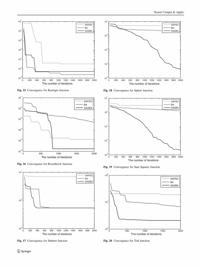
Now, let us first show the convergence rates of all three

algorithms for a given function. For the 20 benchmark

functions, their convergence rates are shown below in

Figs. 2, 3, 4, 5, 6, 7, 8, 9, 10, 11, 12, 13, 14, 15, 16, 17, 18,

19, 20, 21. The horizontal axis shows the number of iter-

ations, and the vertical axis shows the logarithmic value of

the fitness [i.e., log (fitness value)].

Figures 2, 3, 4, 5, 6, 7, 8, 9, 10, 11, 12, 13, 14, 15, 16,

17, 18, 19, 20, 21 show the convergence curves of the 20

test benchmarks using BA, SAPSO and SAGBA, respec-

tively. It can be seen clearly from the pictures that the

convergence rate of SAGBA is obviously faster than those

of the other two algorithms.

By looking at the convergence curves closely, we can

conclude that SAGBA can obtain better results with high

accuracy and steeper convergence rates, compared with the

other two algorithms.

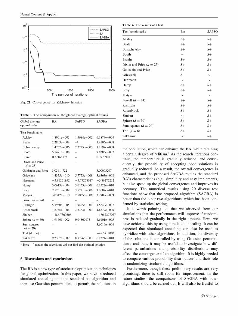
Obviously, the comparison of the convergence curves is

just one way of presenting results. Another way is to

compare the best values found by each algorithm for a

fixed number of iterations. As we have set the number of

iterations to 2,000, the mean values of 50 runs under the

same conditions of numerical experiments are summarized

in Table 3.

In Table 3, ‘-’indicates that the mean minimum value

was not found in the experiments when the max number of

iterations is 2,000 times and the number of running is 50

times.

0 200 400 600 800 1000 1200 1400 1600 1800 200010

-4

10-3

10-2

10-1

100

The number of iterations

SAPSO

BASAGBA

Fig. 2 Convergence for Ackley function

0 200 400 600 800 1000 1200 1400 1600 1800 200010

-8

10-6

10-4

10-2

100

102


SAPSO

BASAGBA

Fig. 3 Convergence for Beale function

0 500 1000 1500 200010

-7

10-6

10-5

10-4

10-3

10-2

10-1


SAPSO

BASAGBA

Fig. 4 Convergence for Bohachevsky function

0 200 400 600 800 1000 1200 1400 1600 1800 200010

-8

10-6

10-4

10-2

100

102


SAPSO

BASAGBA

Fig. 5 Convergence for Booth function


123

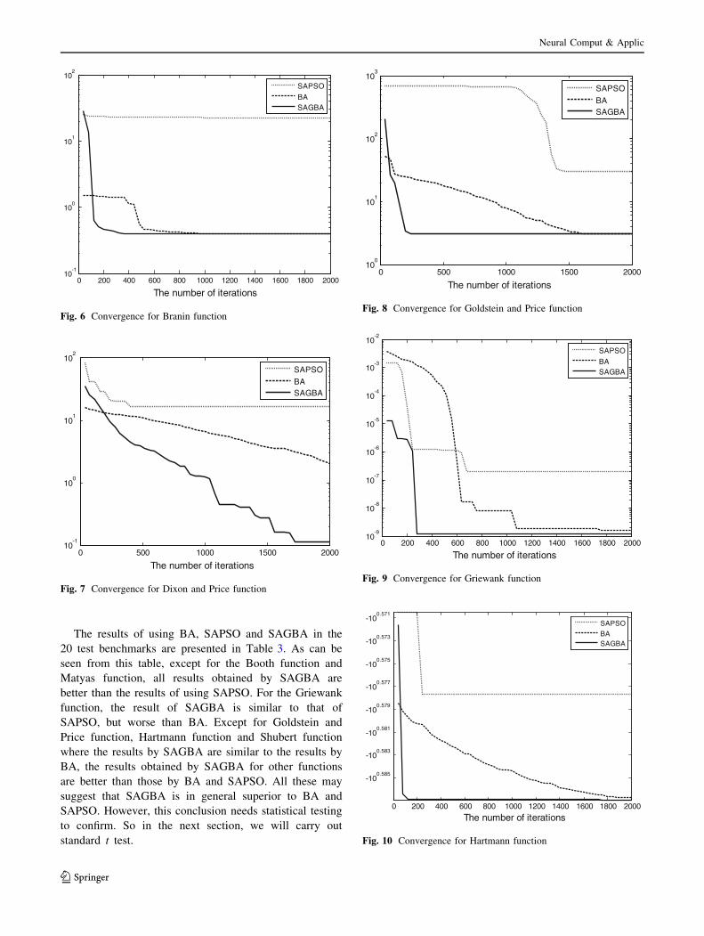
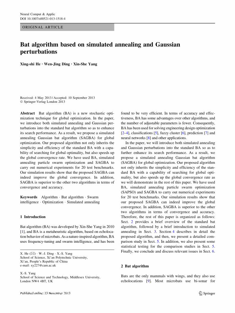
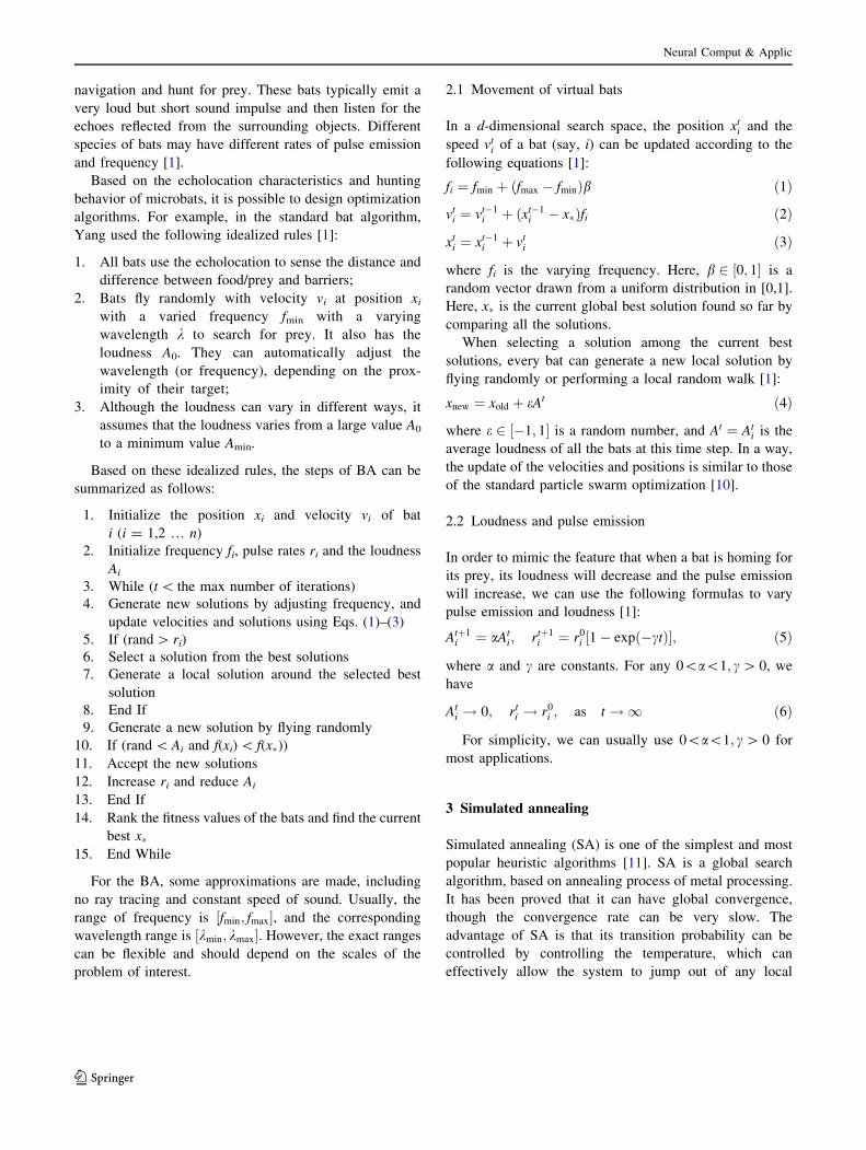
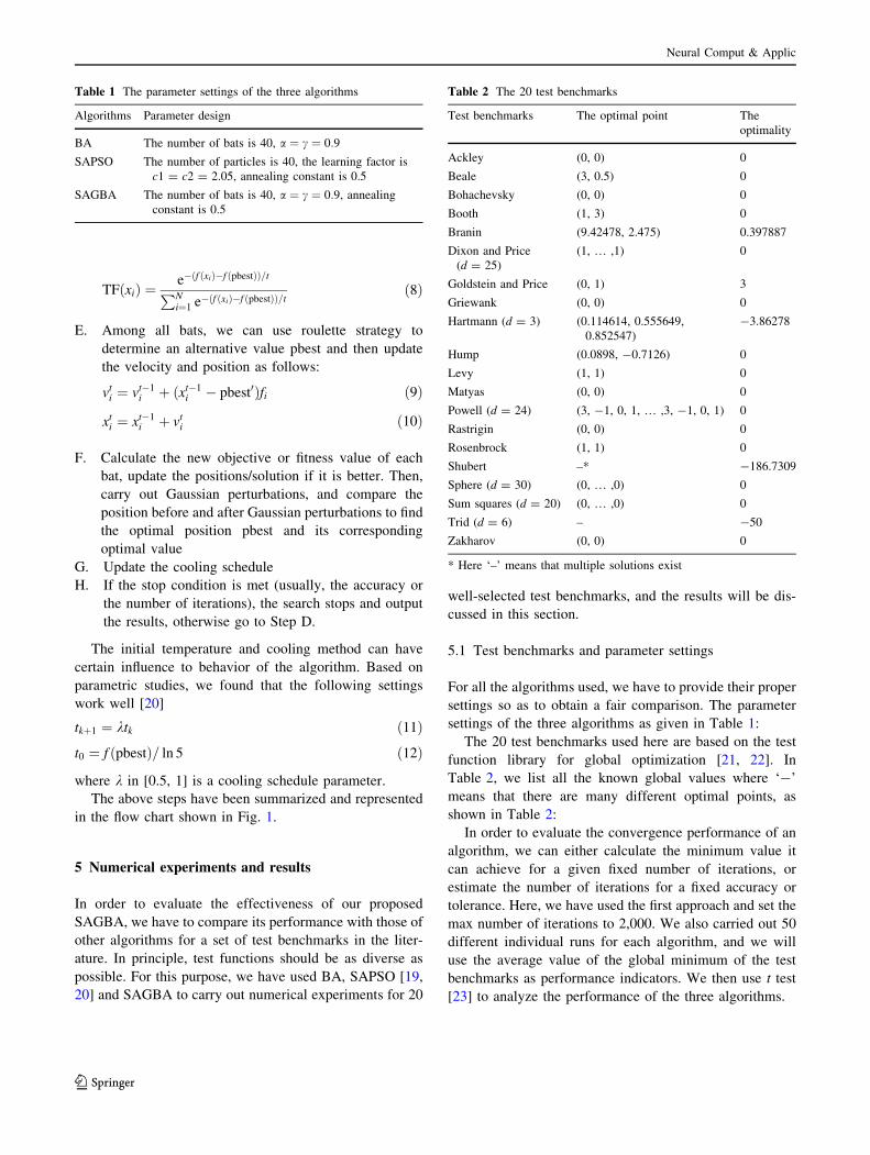
The results of using BA, SAPSO and SAGBA in the

20 test benchmarks are presented in Table 3. As can be

seen from this table, except for the Booth function and

Matyas function, all results obtained by SAGBA are

better than the results of using SAPSO. For the Griewank

function, the result of SAGBA is similar to that of

SAPSO, but worse than BA. Except for Goldstein and

Price function, Hartmann function and Shubert function

where the results by SAGBA are similar to the results by

BA, the results obtained by SAGBA for other functions

are better than those by BA and SAPSO. All these may

suggest that SAGBA is in general superior to BA and

SAPSO. However, this conclusion needs statistical testing

to confirm. So in the next section, we will carry out

standard t test.

0 200 400 600 800 1000 1200 1400 1600 1800 200010

-1

100

101

102


SAPSO

BASAGBA

Fig. 6 Convergence for Branin function

0 500 1000 1500 200010

-1

100

101

102


SAPSO

BASAGBA

Fig. 7 Convergence for Dixon and Price function

0 500 1000 1500 200010

0

101

102

103


SAPSO

BASAGBA

Fig. 8 Convergence for Goldstein and Price function

0 200 400 600 800 1000 1200 1400 1600 1800 200010

-9

10-8

10-7

10-6

10-5

10-4

10-3

10-2


SAPSO

BASAGBA

Fig. 9 Convergence for Griewank function

0 200 400 600 800 1000 1200 1400 1600 1800 2000

-100.571

-100.573

-100.575

-100.577

-100.579

-100.581

-100.583

-100.585


SAPSO

BASAGBA

Fig. 10 Convergence for Hartmann function


123

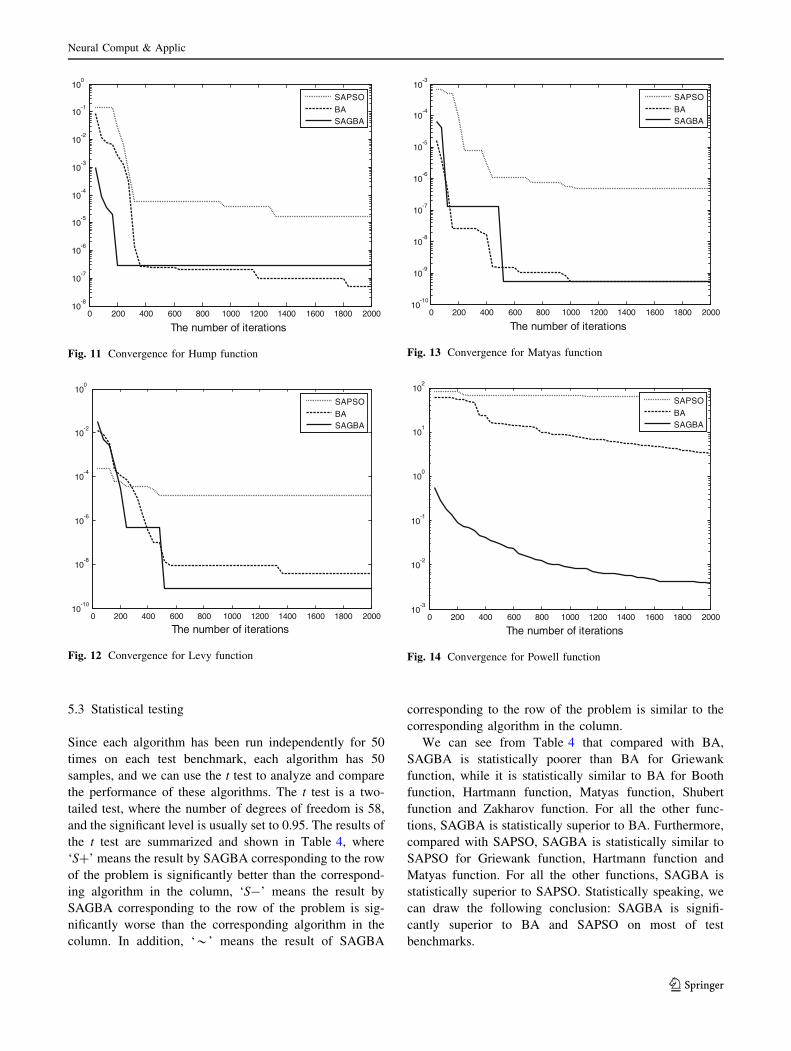
5.3 Statistical testing

Since each algorithm has been run independently for 50

times on each test benchmark, each algorithm has 50

samples, and we can use the t test to analyze and compare

the performance of these algorithms. The t test is a two-

tailed test, where the number of degrees of freedom is 58,

and the significant level is usually set to 0.95. The results of

the t test are summarized and shown in Table 4, where

‘S?’ means the result by SAGBA corresponding to the row

of the problem is significantly better than the correspond-

ing algorithm in the column, ‘S-’ means the result by

SAGBA corresponding to the row of the problem is sig-

nificantly worse than the corresponding algorithm in the

column. In addition, ‘*’ means the result of SAGBA

corresponding to the row of the problem is similar to the

corresponding algorithm in the column.

We can see from Table 4 that compared with BA,

SAGBA is statistically poorer than BA for Griewank

function, while it is statistically similar to BA for Booth

function, Hartmann function, Matyas function, Shubert

function and Zakharov function. For all the other func-

tions, SAGBA is statistically superior to BA. Furthermore,

compared with SAPSO, SAGBA is statistically similar to

SAPSO for Griewank function, Hartmann function and

Matyas function. For all the other functions, SAGBA is

statistically superior to SAPSO. Statistically speaking, we

can draw the following conclusion: SAGBA is signifi-

cantly superior to BA and SAPSO on most of test

benchmarks.

0 200 400 600 800 1000 1200 1400 1600 1800 200010

-8

10-7

10-6

10-5

10-4

10-3

10-2

10-1

100


SAPSO

BASAGBA

Fig. 11 Convergence for Hump function

0 200 400 600 800 1000 1200 1400 1600 1800 200010

-10

10-8

10-6

10-4

10-2

100


SAPSO

BASAGBA

Fig. 12 Convergence for Levy function

0 200 400 600 800 1000 1200 1400 1600 1800 200010

-10

10-9

10-8

10-7

10-6

10-5

10-4

10-3


SAPSO

BASAGBA

Fig. 13 Convergence for Matyas function

0 200 400 600 800 1000 1200 1400 1600 1800 200010

-3

10-2

10-1

100

101

102


SAPSO

BASAGBA

Fig. 14 Convergence for Powell function


123

0 200 400 600 800 1000 1200 1400 1600 1800 200010

-6

10-5

10-4

10-3

10-2

10-1

100


SAPSO

BASAGBA

Fig. 15 Convergence for Rastrigin function

0 500 1000 1500 200010

-6

10-5

10-4

10-3

10-2

10-1


SAPSO

BASAGBA

Fig. 16 Convergence for Rosenbrock function

0 200 400 600 800 1000 1200 1400 1600 1800 2000-10

3

-102

-101


SAPSO

BASAGBA

Fig. 17 Convergence for Shubert function

0 200 400 600 800 1000 1200 1400 1600 1800 200010

-5

10-4

10-3

10-2

10-1


SAPSO

BASAGBA

Fig. 18 Convergence for Sphere function

0 200 400 600 800 1000 1200 1400 1600 1800 200010

-3

10-2

10-1

100

101


SAPSO

BASAGBA

Fig. 19 Convergence for Sum Squares function

0 500 1000 1500 2000-10

2

-101

-100


SAPSO

BASAGBA

Fig. 20 Convergence for Trid function


123

6 Discussions and conclusions

The BA is a new type of stochastic optimization techniques

for global optimization. In this paper, we have introduced

simulated annealing into the standard bat algorithm and

then use Gaussian perturbations to perturb the solutions in

the population, which can enhance the BA, while retaining

a certain degree of ‘elitism.’ As the search iterations con-

tinue, the temperature is gradually reduced, and conse-

quently, the probability of accepting poor solutions is

gradually reduced. As a result, the overall convergence is

enhanced, and the proposed SAGBA retains the standard

BA’s characteristics (e.g., simplicity and easy implement),

but also speed up the global convergence and improves its

accuracy. The numerical results using 20 diverse test

functions show that the proposed algorithm (SAGBA) is

better than the other two algorithms, which has been con-

firmed by statistical testing.

It is worth pointing out that we observed from our

simulations that the performance will improve if random-

ness is reduced gradually in the right amount. Here, we

have achieved this by using simulated annealing. It can be

expected that simulated annealing can also be used to

hybridize with other algorithms. In addition, the diversity

of the solutions is controlled by using Gaussian perturba-

tions, and thus, it may be useful to investigate how dif-

ferent perturbations and probability distributions may

affect the convergence of an algorithm. It is highly needed

to compare various probability distributions and their role

in randomizing stochastic algorithms.

Furthermore, though these preliminary results are very

promising, there is still room for improvement. In the

future studies, the comparisons of SAGBA with other

algorithms should be carried out. It will also be fruitful to

0 500 1000 1500 200010

-10

10-8

10-6

10-4

10-2

100


SAPSO

BASAGBA

Fig. 21 Convergence for Zakharov function

Table 3 The comparison of the global average optimal values

Global average

optimal value

BA SAPSO SAGBA

Test benchmarks

Ackley 1.8001e-003 1.5684e-003 6.1879e-004

Beale 2.2803e-004 –* 1.4105e-008

Bohachevsky 1.4737e-006 2.2725e-005 1.1597e-008

Booth 5.5471e-008 – 9.8286e-007

Branin 0.77166193 – 0.39789001

Dixon and Price

(d = 25)

– – –

Goldstein and Price 3.03614722 – 3.00003207

Griewank 1.4375e-010 5.7773e-008 3.6363e-008

Hartmann -3.86261952 -3.77258017 -3.86272212

Hump 5.0613e-004 5.0153e-008 6.1522e-010

Levy 2.5251e-009 3.5721e-006 1.7607e-010

Matyas 3.0342e-010 2.5055e-006 3.7909e-009

Powell (d = 24) – – –

Rastrigin 5.5960e-005 1.9425e-004 1.5840e-007

Rosenbrock 7.8735e-004 3.5383e-003 4.6779e-006

Shubert -186.7309306 – -186.7297027

Sphere (d = 30) 1.91766-003 0.04860173 4.6101e-005

Sum squares

(d = 20)

– – 3.6016e-004

Trid (d = 6) – – -49.5717002

Zakharov 9.2307e-009 8.7796e-003 6.1224e-010

* Here ‘–’ means the algorithm did not find the optimal solution

Table 4 The results of t test

Test benchmarks BA SAPSO

Ackley S? S?

Beale S? S?

Bohachevsky S? S?

Booth * S?

Branin S? S?

Dixon and Price (d = 25) S? S?

Goldstein and Price S? S?

Griewank S- *

Hartmann * *

Hump S? S?

Levy S? S?

Matyas * *

Powell (d = 24) S? S?

Rastrigin S? S?

Rosenbrock S? S?

Shubert * S?

Sphere (d = 30) S? S?

Sum squares (d = 20) S? S?

Trid (d = 6) S? S?

Zakharov * S?


123

apply SAGBA to multi-objective optimization. In addition,

it will be extremely useful to apply the proposed algorithm

to large-scale real-world design problems in engineering.

Acknowledgments The authors would like to thank the financial

support by Shaanxi Provincial Soft Science Foundation

(2012KRM58) and Shaanxi Provincial Education Grant (12JK0744

and 11JK0188).

References

1. Yang XS (2010) A new metaheuristic bat-inspired algorithm. In:

Nature inspired cooperative strategies for optimization (NICSO),

vol 284. Springer, SCI, pp 65–74

2. Yang XS (2011) Bat algorithm for multi-objective optimization.

Int J Bio Inspired Comput 3(5):267–274

3. Li ZY, Ma L, Zhang HZ (2012) Genetic mutation bat algorithm

for 0–1 knapsack problem. Comput Eng Appl 2012(35):1–10 (in

Chinese)

4. Lemma TA (2011) Use of fuzzy systems and bat algorithm for

energy modeling in a gas turbine generator. In: IEEE Colloquium

on Humanities, Science and Engineering, pp 305–310

5. Yang XS, Gandomi AH (2012) Bat algorithm: a novel approach

for global engineering optimization. Eng Comput 29(5):464–483

6. Mishra S, Shaw K, Mishra D (2012) A new metaheuristic clas-

sification approach for microarray data. Procedia Technol

4:802–806

7. Khan K, Nikov A, Sahai A (2011) A fuzzy bat clustering method

for ergonomic screening of office workplaces, S3T 2011. Adv

Intell Soft Comput 101:59–66

8. Khan K, Sahai A (2012) A comparison of BA, GA, PSO, BP and

LM for training feed forward neural networks in e-learning

context. Int J Intell Syst Appl (IJISA) 4(7):23–29

9. Altringham JD (1996) Bats: biology and behaviour. Oxford

University Press, Oxford

10. Kennedy J, Eberhart R (1995) Particle swarm optimization. In:

IEEE, International Conference on Neural Networks, Perth,

Australia

11. Bertsimas D, Tsitsiklis J (1993) Simulated annealing. Int Stat Sci

8(1):10–15

12. Zhiyuan W, Huihe S, Xinyu W (1997) Genetic annealing evo-

lutionary algorithm. J ShangHai JiaoTong University (in China)

31(12):69–71

13. Xuemei Wang, Yihe Wang (1997) The combination of simulated

annealing and genetic algorithms. Chin J Comput (in China)

20(4):381–384

14. Yang XS (2011) Review of meta-heuristic and generalised evo-

lutionary walk algorithm. Int J Bio-Inspired Comput 3(2):77–84

15. Gandomi AH, Yun GJ, Yang XS, Talatahari S (2013) Chaos-

enhanced accelerated particle swarm optimization. Commun

Nonlinear Sci Numer Simul 18(2):327–340

16. Yang XS, Deb S (2012) Two-stage eagle strategy with differ-

ential evolution. Int J Bio-Inspired Comput 4(1):1–5

17. Yang XS, Deb S (2013) Multiobjective cuckoo search for design

optimization. Comput Oper Res 40(6):1616–1624

18. Gandomi AH, Yang XS, Talatahari S, Deb S (2012) Coupled

eagle strategy and differential evolution for unconstrained and

constrained global optimization. Comput Math Appl 63(1):

191–200

19. Zhao S, Huang G (2006) Design and study of particle swarm

optimization with simulated annealing. J Baise University

19(6):9–12

20. Gong C, Wang Z (2009) Proficient in MATLAB. Beijing: Pub-

lishing House of Electronics Industry (in China), pp 309–312

21. Hedar J Test functions for unconstrained global optimization

[DB/OL]. http://www-optima.amp.i.kyoto-u.ac.jp/member/student/

hedar/Hedar_files/TestGO_files/Page364.htm

22. Jamil M, Yang XS (2013) A literature survey of benchmark

functions for global optimization problems. Int J Math Model

Numer Optim 4(2):150–194

23. Fisher RA (1925) Theory of statistical estimation. Proceed Camb

Philos Soc 22:700–715


123

http://www-optima.amp.i.kyoto-u.ac.jp/member/student/hedar/Hedar_files/TestGO_files/Page364.htm

http://www-optima.amp.i.kyoto-u.ac.jp/member/student/hedar/Hedar_files/TestGO_files/Page364.htm

bat algorithm based on simulated annealing and gaussian perturbations

Documents