basis functions and basis sets - folk.uio.nofolk.uio.no/helgaker/talks/sostrupbasis_10.pdf · basis...

Basis functions and basis sets

Trygve Helgaker

Centre for Theoretical and Computational ChemistryDepartment of Chemistry, University of Oslo, Norway

The 11th Sostrup Summer SchoolQuantum Chemistry and Molecular Properties

July 4–16 2010

Trygve Helgaker (CTCC, University of Oslo) Basis functions and basis sets 11th Sostrup Summer School (2010) 1 / 24

One-electron basis functions

I Molecular orbitals (MOs) may be constructedI numerically: flexible but intractableI algebraically by expansion in simple one-electron basis functions

φp(r) =∑µ

Cµpχµ(r)

I What are the requirements on the basis functions?I they should provide a systematic extension towards completenessI they should give a rapid convergence for any electronic stateI they should be easy to integrate over

I It is difficult to satsify all these requirementsI some compromise must be sought . . .

I We shall always insist on completeness of our basis functionsI completeness in one-electron space ensures completeness in (FCI) N-electron spaceI in practice, we will always use incomplete basis setsI however, these must be systematically extendable towards completeness

I Overview:I general considerationsI angular functions (spherical harmonics)I radial functions (STOs and GTOs)

Trygve Helgaker (CTCC, University of Oslo) Introduction 11th Sostrup Summer School (2010) 2 / 24

One- and many-center molecular expansions

One-center molecular expansions

I Mathematically, it is easy to set up one-center expansions that are

I universal and uniquely definedI complete, discrete and orthonormal

I Convergence is invariably slow since little physics has been built into the basis

Many-center molecular expansions

I Atoms retain much of their identity in molecules

I atomic electron distributions are largely unaffected by bonding

I We therefore combine separate one-electron bases for each atom in the molecule

I The molecular orbitals are thus constructed from atomic orbitals (AOs)

I better convergenceI uniform qualityI less systematicI linear dependencies

Trygve Helgaker (CTCC, University of Oslo) Introduction 11th Sostrup Summer School (2010) 3 / 24

Central-field systems

I We shall develop AOs by considering one-electron central-field systems:

−1

2∇2ψ(r) + V (r)ψ(r) = Eψ(r) ← V (r) spherically symmetric

I Their wave functions may be separated into radial and angular parts:

ψn`m(r , θ, ϕ) = Rn`(r)Y`m(θ, ϕ)

I The angular solutions are universal:

Y`m(θ, ϕ) ← spherical harmonics

and constitute a complete set on L2(S)∫ 2π

0

∫ π

0Y ∗`m(θ, ϕ)Y`′m′ (θ, ϕ) sin θ dθ dϕ = δ``′δmm′

I By contrast, the radial solutions depend on the potential:

−1

2

d2rRn`(r)

dr2+

[V (r) +

`(`+ 1)

2r2

]rRn`(r) = ErRn`(r)

and constitute a complete set on L2(R+, r2)∫ ∞0

R∗m`(r)Rn`(r)r2 dr = δmn

Trygve Helgaker (CTCC, University of Oslo) Central-field systems 11th Sostrup Summer School (2010) 4 / 24

From spherical to solid harmonics

I The radial forms of the AOs always contain the monomial r`:

Rn`(r) = r`Rn`(r)

I We therefore introduce the solid harmonics:

Y`m(r , θ, ϕ) = r`Y`m(θ, ϕ)

I To avoid complex algebra, we note that

Y∗`m = (−1)mY`,−m

and introduce the real-valued solid harmonics

S`|m| + iS`,−|m| = (−1)m

√8π

2`+ 1Y`m

I The real-valued solid harmonics S`m(s, y , z) for ` ≤ 2:

m \ ` 0 1 2

2 12

√3(x2 − y2

)1 x

√3xz

0 1 z 12

(3z2 − r2

)−1 y

√3yz

−2√

3xy


Radial forms

I The general form of the one-electron functions is

ψn`m(r , θ, φ) = Rn`(r)Y`m(θ, ϕ)

I A variety of radial functions are in use of the general form

[ a polynomial in r ]× [ a decaying function in r ]

I There are two main classes of radial functions:

I exponential functionsRn`(r) = r`Pn−`−1(r) exp(−ζr)

I Gaussian functionsRn`(r) = r`Pn−`−1(r2) exp(−αr2)

I Flexibility in the radial part is obtained by

I use of the principal quantum number nI use of variable exponents ζ and α


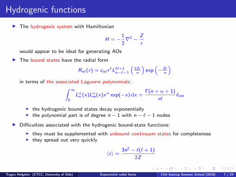
Hydrogenic functions

I The hydrogenic system with Hamiltonian

H = −1

2∇2 −

Z

r

would appear to be ideal for generating AOs

I The bound states have the radial form

Rn`(r) = cn`r`L2`+1

n−`−1

(2Zrn

)exp

(− Zr

n

)in terms of the associated Laguerre polynomials:∫ ∞

0Lαn (x)Lαm(x)xα exp(−x) dx =

Γ(n + α+ 1)

n!δnm

I the hydrogenic bound states decay exponentiallyI the polynomial part is of degree n − 1 with n − `− 1 nodes

I Difficulties associated with the hydrogenic bound-state functions:

I they must be supplemented with unbound continuum states for completenessI they spread out very quickly

〈r〉 =3n2 − `(`+ 1)

2Z

Trygve Helgaker (CTCC, University of Oslo) Exponential radial forms 11th Sostrup Summer School (2010) 7 / 24

The Laguerre functions

I For a fixed exponent ζ, the Laguerre functions

RLFn` = cLF

n` r`L2`+2

n−`−1 (2ζr) exp (−ζr)

constitute a complete, discrete set in L2(R+, r2)

I They retain the exponential decay of the hydrogenic functions

Rn`(r) = cn`r`L2`+1

n−`−1

(2Zrn

)exp

(− Zr

n

)while avoiding the continuum

I They are much more compact than the hydrogenic functions: 〈r〉 = (2n + 1)/ζ

0 10 20

1s

0 10 20

2s

0 10 20

3s

0 10 20

2p

0 10 20

3p

0 10 20

3d


Expansion of carbon orbitals in Laguerre functionsI Least-squares fits to the numerical carbon 3P ground-state orbitals

I RLFn` expansions with n ≤ 2, 8, 15 and fixed exponent ζ = 1:

1 2 3 4 5

1.0

2.0

3.0

1s

1 2 3 4 5

0.2

0.4

0.6

2s

1 2 3 4 5

0.1

0.3

0.5

2p

2 8 150.0

0.5

1.0

1s2s2p

I convergence is guaranteed but slowI functions with a fixed exponent are ill suited for widely different radial distributions

I Solution: use functions with variable exponents adapted to the system

〈r〉 =2n + 1

ζ


Slater-type orbitals (STOs)I With variable exponents, orthogonality is lost even in atomic systems

I there is no need to retain the nodal structure of the Laguerre functionsI Slater-type orbitals (STOs) are obtained by retaining only the highest monomial:

RLFn` = r`L2`+2

n−`−1 (2ζr) exp (−ζr) → RSTOn` = rn−1 exp (−ζr)

I note the simple structure of the STOs:

1s = exp(−ζr)

2s = r exp(−ζr)

2p0 = z exp(−ζr)

3s = r2 exp(−ζr)

3p0 = zr exp(−ζr)

3d0 =(3z2 − r2) exp(−ζr)

I For a fixed ζ, the STOs constitute a complete, discrete set of one-electron functions

I But radial flexibility may also by obtained with variable exponents: 〈r〉 = (2n + 1)/ζ

1 3 5 7 9

0.2

0.4

1sH1L

2sH1L3sH1L

1 3 5 7 9

0.2

0.4

1sH1L

1sH1�2L

1sH1�3L


STO basis sets

I In practice, n and ζ are used in combination to ensure radial flexibility:

I Minimal STO basis for carbon:

1s = exp(−5.88r), 2s = r exp(−1.57r), 2p0 = z exp(−1.46r)

1 2 3 4

1.5

3.01s

1 2 3 4

0.3

0.62s

1 2 3 4

0.3

0.62p

I Extended STO basis for carbon:

STO type exponents 1s 1s 2p1s STO 9.2863 0.07657 −0.01196

5.4125 0.92604 −0.210412s STO 4.2595 0.00210 −0.13209

2.5897 0.00638 0.346241.5020 0.00167 0.741081.0311 −0.00073 0.06495

2p STO 6.3438 0.010902.5873 0.235631.4209 0.577740.9554 0.24756


Gaussian radial forms

I Boys introduced Gaussians as molecular basis functions in 1950

I his motivation was to simplify integrationI Gaussians do not have a nuclear cusp and decay too rapidlyI nevertheless, they constitute a complete set of functions

I For STOs, we proceeded by

1 identifying a complete, discrete set of radial functions: Laguerre functions2 simplifying their nodal structure: STOs3 ensuring radial flexibility by a use of n and variable exponent ζ

I For GTOs, we shall proceed in the same manner by

1 identifying a complete, discrete set of radial functions: harmonic-oscillator functions2 simplifying their nodal structure: GTOs3 ensuring radial flexibility by use of variable exponents only

Trygve Helgaker (CTCC, University of Oslo) Gaussian radial forms 11th Sostrup Summer School (2010) 12 / 24

Harmonic-oscillator (HO) functionsI For a fixed α, the three-dimensional harmonic-oscillator (HO) Hamiltonian

H = −1

2∇2 +

1

2(2α)2 r2

has the following complete set of Gaussian radial solutions:

RHOn` = cHO

n` r`L`+1/2n−`−1

(2αr2

)exp

(−α2r2

)I Note: the HO functions are obtained from the LF functions

RLFn` = cLF

n` r`L2`+2

n−`−1 (2ζr) exp (−ζr)

by globally substituting r2 for r in the radial part and adjusting for orthonormality

I the HO nodal structure is the same as for the LF functions

2 4 6

1

3

5

1s

2 4 6

1

3

5

2s

2 4 6

1

3

5

3s

2 4 6

1

3

5

2p

2 4 6

1

3

5

3p

2 4 6

1

3

5

3d


GTOs: nodeless HO functions

I Dispensing with the HO nodes, we obtain the Gaussian-type orbitals (GTOs):

RGTOn` (r) = cGTO

n` r`r2(n−`−1) exp(−αr2)

I like the HO functions, the GTOs form a complete, discrete set for fixed α

I A comparison of STOs and GTOs:

STO GTO1s exp (−ζr) exp

(−αr2

)2s r exp (−ζr) r2 exp

(−αr2

)2p0 z exp (−ζr) z exp

(−αr2

)3s r2 exp (−ζr) r4 exp

(−αr2

)3p0 zr exp (−ζr) zr2 exp

(−αr2

)3d0

(3z2 − r2

)exp (−ζr)

(3z2 − r2

)exp

(−αr2

)

0 1 2 3 4 5

1

2

1s

2s3s

0 1 2 3 4 5

1

2

1s

2s

3s


Spherical-harmonic GTOs

I For GTOs with a fixed exponent, convergence is exceedingly slow

I radial space must instead be spanned by variable exponents

〈r〉GTO ≈√

2n−`−22α

, 〈r〉STO = 2n+1ζ

1 2 3

0.5

1.0

1sH1L 2sH1L

3sH1L

1 2 3

0.5

1.01sH1L

1sH1�2L

1sH1�3L

I Indeed, the radial space is usually spanned entirely by variable exponents

I we thus employ solid-harmonic GTOs with only two quantum numbers:

Gα,`m(r , θ, ϕ) = S`m(r , θ, ϕ) exp(−αr2

)discarding GTOs with n > `+ 1 such as the 2s function r2 exp

(−αr2

)I Completeness is ensured by selecting the exponents in a special manner

I for example, using exponents such as n−1 and n−1/2 for n = 1, 2, 3 . . .I in practice, such criteria are not very useful


Molecular basis sets: some general comments

I Requirements for correlated and uncorrelated wave-function models are different

I uncorrelated models require an accurate representation of the one-electron densityI correlated models require also an accurate representation of the two-electron density

I Requirements vary also for different molecular properties

I energy-optimized basis sets have most flexibility in the valence regionI many properties depend on flexibility in other regions such as

I the outer valence region for electric propertiesI the inner core region for nuclear field gradients

I It is impossible to develop basis sets that are universal, applicable in all situations

I we here concentrate on basis sets for uncorrelated energy calculationsI we will study basis sets for correlated energies after a discussion of the Coulomb hole

I Overview of our discussion of basis sets for uncorrelated calculations:

1 STO-kG2 primitive GTOs from Hartree–Fock calculations3 even-tempered basis sets4 contracted basis setes5 polarization functions6 benchmarking

Trygve Helgaker (CTCC, University of Oslo) Molecular basis sets 11th Sostrup Summer School (2010) 16 / 24

STO-kG basis setsI In the STO-kG basis sets, STOs are expanded in fixed linear combinations of GTOs:

χSTOn`m =

k∑i=1

diχGTOα,`m

I STOs are retained as the conceptual basisI GTOs are introduced to simplify integration

I The following basis functions are obtained by least-squares fitting:

1 2 3 4

0.2

0.4

0.6STO-1G

1 2 3 4

0.2

0.4

0.6STO-2G

1 2 3 4

0.2

0.4

0.6STO-3G

1 2 3 4

0.2

0.4

0.6STO-4G

1 2 3 4

0.2

0.4

0.6STO-5G

1 2 3 4

0.2

0.4

0.6STO-6G

I these fits are only needed for ζ = 1I scaling gives functions for ζ 6= 1

I The STO-3G basis sets are only useful for exploratory investigations


GTO basis sets by energy minimization

I Treating the GTOs as primary basis, their exponents must be determined independently

I the most obvious approach is by minimization of atomic energies

I A large number of such primitive GTOs are needed for good accuracy

I example: Huzinaga 9s5p:

1 2 3 4 5

1

2

31s

1 2 3 4 5

0.2

0.4

0.62s

1 2 3 4 5

0.2

0.4

0.62p

I Errors in the electronic energy:

basis error (mEh)STO-3G 460STO-6G 79.6

9s5p 3.4DZ STO 1.9

10s6p 1.3


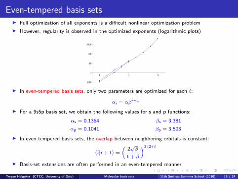
Even-tempered basis setsI Full optimization of all exponents is a difficult nonlinear optimization problem

I However, regularity is observed in the optimized exponents (logarithmic plots)

1 5 9

1�10

1

10

100

1000

I In even-tempered basis sets, only two parameters are optimized for each `:

αi = αβi−1

I For a 9s5p basis set, we obtain the following values for s and p functions:

αs = 0.1364 βs = 3.381

αp = 0.1041 βp = 3.503

I In even-tempered basis sets, the overlap between neighboring orbitals is constant:

〈i |i + 1〉 =

(2√β

1 + β

)3/2+`

I Basis-set extensions are often performed in an even-tempered manner


Contracted GTOs

I To describe atomic orbitals accurately, a large number of GTOs are needed

I upon bond formation, the electron distribution does not usually change muchI there is no need to employ all GTOs individually in the molecular calculations

I Instead, we use contracted GTOs: fixed linear combinations of primitive GTOs

RCGTOα (r) =

∑i

dαiRGTOαi

(r)

I Segmented contraction

I each primitive contributes to just one contracted

I General contraction

I each primitive contributes to all contracted of same symmetry


Dunning’s contracted basis sets

I Dunning’s contracted functions are based on a primitive basis optimized by Huzinaga

I The coefficients (here for carbon) are not reoptimized upon contraction

exponents [3s] [4s] [5s] [2p] [3p]

4232.61 0.002029 0.002029 0.006228634.882 0.015535 0.015535 0.047676146.097 0.075411 0.075411 0.23143942.4974 0.257121 0.257121 0.78910814.1892 0.596555 0.596555 0.791751

1.9666 0.242517 0.242517 0.3218705.1477 1.000000 1.000000 1.0000000.4962 0.542048 1.000000 1.0000000.1533 0.517121 1.000000 1.000000

18.1557 0.018534 0.0391963.9864 0.115442 0.2441441.1429 0.386206 0.8167750.3594 0.640089 1.0000000.1146 1.000000 1.000000

I Plots of the [5s3p] contractions s and p functions:

1 2 3 4

1

2

3

4

1 2 3 4 5 6

0.2

0.4

0.6

0.8


Pople’s 6-31G basisI In the Pople-type basis sets, exponents and coefficients are simultaneously optimized

I Example: the 6-31G split-valence basis for carbonI note: shared exponents for 2s and 2p

exponents 1s 2s 2p3047.52 0.00183474

457.37 0.0140373103.949 0.068842629.2102 0.2321849.28666 0.4679413.16393 0.3623127.86827 −0.119332 0.06899911.88129 −0.160854 0.316424

0.544249 1.14346 0.7443080.168714 1.0000 1.0000

I Plots of s and p functions:

1 2 3 4

1

2

3

4

1 2 3 4 5 6

0.2

0.4

0.6

0.8


Polarization functions

I Up to now, we have used AOs of same symmetry as the occupied atomic orbitals

I in molecules, the atomic density is distorted and spherical symmetry broken

I To describe this distortion, we include polarization functions

I AOs of angular momentum higher than those of the occupied atomic orbitals

I Example: distortion of the 1s function:

s(A) = exp(−αr2

A

)s(A + δz ) = s(A) + 2αzAs(A)δz + · · ·

= s(A) + 2αδzpz (A) + · · ·

I Choose the exponent so that the polarization function contributes most where the chargedensity has a maximum

αpol`+1 =

`+ 2

`+ 1α`

I Examples: DZP, 6-31G*


Basis-set convergence in Hartree–Fock theoryI For basis sets to be useful, their performance must be examined systematically

I For high accuracy and for establishing error bars, a series of calculations is necessary

basis set ∆ENe ∆EN2∆EH2O RNN ROH θHOH

STO-3G 1942.57 1497.29 1104.47 146.82 98.94 100.036-31G 73.22 125.43 83.40 108.91 94.96 111.556-311G 24.54 99.02 58.01 108.60 94.54 111.886-31G∗ 73.22 51.32 58.27 107.81 94.76 105.586-31G∗∗ 73.22 51.32 44.75 107.81 94.27 106.056-311G∗∗ 24.54 23.76 20.95 107.03 94.10 105.46cc-pVDZ 58.32 39.06 40.60 107.73 94.63 104.61cc-pVTZ 15.23 9.72 10.23 106.71 94.06 106.00cc-pVQZ 3.62 2.11 2.57 106.56 93.96 106.22cc-pV5Z 0.32 0.43 0.31 106.54 93.96 106.33cc-pCVDZ 58.17 38.27 40.20 107.65 94.60 104.64cc-pCVTZ 15.14 8.79 10.04 106.60 94.05 106.00cc-pCVQZ 3.52 1.88 2.45 106.55 93.96 106.22cc-pCV5Z 0.32 0.36 0.30 106.54 93.96 106.33

I Some comments:

I STO-3G performs very poorlyI 6-31G gives qualitative accuracy (but not for the bond angle)I 6-311G improves only the energyI 6-31G* contains polarization functions and improves the geometryI correlation-consistent basis sets (studied later) converge smoothly and rapidly


basis functions and basis sets - folk.uio.nofolk.uio.no/helgaker/talks/sostrupbasis_10.pdf · basis...

Documents