basics of probability theory - intranet...

Basics of Probability Theory

Antonio Capone

Politecnico di Milano

Antonio Capone (Politecnico di Milano) Basics of Probability Theory 1 / 93

Content

1 ProbabilitiesDefinitionsUniform spacesConditional spacesBayes’ FormulasStatistical independence

2 Random VariablesSpaces with infinite outcomesContinuous Random VariablesDiscrete Random VariablesMoments of a pdfConditional distributions and densitiesVectorial Random VariablesFunctions of Random Variables


Probabilities

Probabilities




Probabilities Definitions

Basic definitions

Probability theory provides a mathematical description of the possibleoutcomes of experiments. Let E be an experiment which provides a finitenumber of outcomes α1, α2, . . . , αn.We have the following definitions:

Trial is the execution of E which leads to a outcome, or sample, αand only one.

Space or stochastic universe associated with the experiment E isthe set S = α1, α2, . . . .αn of all possible outcomes of E .

Event is any set A of outcomes and what is a any subset of S .

An Elementary Event (or Sample Event) is a set E ⊂ S with asingle outcome.



Basic definitions

(cont’d) definitions:

A Certain Event is the event corresponding to S .

The Impossible Event is the empty set ∅.Events can be combined with operations in use in Set theory,obtaining events such as union (or sum) events, conjunction (orproduct or intersection) events, complement events, and differenceevents.

We say that in a trial event A occurs if the outcome of the trialbelongs to A.



Basic properties

Some basic properties directly follow from definitions:

The certain event always occurs;

The impossible event never occurs;

A union event occurs if at least one of the component events occurs;

A joint event occurs if all the components events occursimultaneously;

Disjoint events can not occur simultaneously, and for this reasonsthey are called mutually exclusive (as for example sample events andcomplementary events).



Probability definition

The probability P(A) of an event A ⊂ S is a measure defined on S so asto satisfy the following axioms:Axiom I: P(A) is a nonnegative real number associated with the event.

P(A) ≥ 0 (1)

Axiom II: the probability of the certain event is one.

P(S) = 1 (2)

Axiom III: if A e B are disjoint events

P(A + B) = P(A) + P(B) (3)



Probability definition

Based on the axioms, probabilities have the following properties:

P(A) = 1− P(A) ≤ 1 (4)

P(φ) = 0 (5)

If B ⊂ A, thenP(B) ≤ P(A) (6)

If A1,A2, . . . ,An are disjoint events, and A = A1 + A2 + . . .+ An, then wehave

P(A) = P(A1) + P(A2) + . . .+ P(An). (7)



Probability space description

A complete stochastic description of an experiment is obtained whena sufficient number of probabilities to events have been assigned

From a mathematical point of view the assignments are arbitrarywithin the limits of the axioms but obviously for applications we useprobability for measuring the likelihood that an event occurs

A formal link between probabilities and occurrence of events inrepeated trials is provided by the law of large numbers (see later).

We say that an experiment E (or probability space S) is completelydescribed from the probabilistic point of view when probabilities are givenfor each elementary event Ei

pi = P(Ei )

The probability of any event A can then be obtained as the sum of theprobabilities of its elementary events.



Uniform spaces

If all the nS elementary events Ei are equally probable, the space S iscalled uniform

For a uniform space S of nS elements, the probability of an event Acomposed of rA elementary events is:

P(A) =rAnS

(8)

Therefore for uniform spaces, probability calculations are performedby counting techniques (as in combinatorial calculus) in order to getrA and nS .


Probabilities Uniform spaces

Urn model

A useful way of describing uniform finite spaces is through the urnmodel

It is an ideal experiment consisting in drawing k objects (elements)from an urn containing n objects (like e.g. numbered or colored balls)

The model assumes that all possible outcomes consisting of all thegroups that can be formed with k out of n objects are equallyprobable



Counting groups

Counting the number of k out of n objects and the number of groupsin a given event allows to completely characterize experiments in theurn model

If groups differ in at least one element or in the order they appear inthe group, and if objects are drawn together or one by one with noreplacement

nS = (n)k = n(n − 1) . . . (n − k + 1) =n!

(n − k)!.

While, if objects are drawn one by one with re-insertion/replacementof the drawn element in the urn

nS = nk



Counting groups

If the order does not count we have to divide by the number k! ofpossible permutations and we get:

nS =

(n

k

)=

(n)kk!

=n!

k!(n − k)!,

in the case of drawn with no replacement, and

nS =nk

k!,

in the case of with replacement.



Example (1)

In an urn there are ten objects representing the ten digits 0, 1, . . . , 9.Evaluate the probability that, upon drawing of 3 elements, the three digitsform the event

A = number 567

B = number with three consecutive increasing digits

We have nS = (10)3 = 10 · 9 · 8 = 720

rA = 1 P(A) =1

720

rB = 8 P(B) =8

720



Example (2)

Like in previous example but assuming that we have three consecutivedrawings with the replacement of the element previously drawn. Evaluatethe probability of events:

A = number 567

B = number with three consecutive increasing digits

C = number with all equal digits.

nS = 103

rA = 1 P(A) =1

1000

rB = 8 P(B) =8

1000

rC = 10 P(C ) =10

1000



Example (3)

Evaluate the minimum number of people k you need to pick so that theprobability of having at least two people born on the same day is greateror equal 0.5.The experiment is equivalent to drawing k numbers out of an urn thatcontains 365 objects, each representing a different day of the year.Denoting with Dk = { extraction k objects all different } we have

P(Dk) =(365)k(365)k

k ≤ 365

The probability that at least two people are born in the same day is:

P(Dk) = 1− P(Dk) = 1− 365!

(365− k)! 365k> 0, 5.

The non linear equation can be solved numerically. The result is k = 23.


Probabilities Conditional spaces

Union of non disjoint events

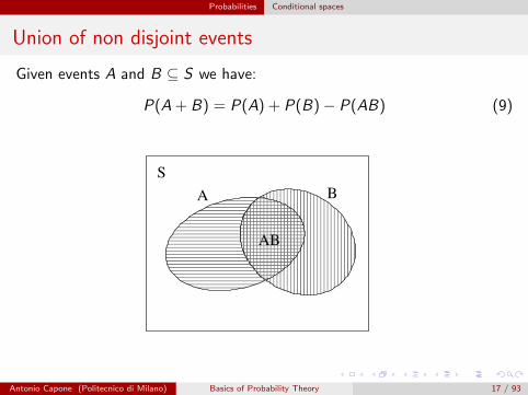
Given events A and B ⊆ S we have:

P(A + B) = P(A) + P(B)− P(AB) (9)

S

A B

AB



Example (4)

In a throw of dice, evaluate the probability that number is either even orless than 3.Denote the event ”even number” as A and the event ”less than three” asB we have

P(D) = P(A + B) = P(A) + P(B)− P(AB),

We evaluate P(A),P(B), and P(AB) with the counting process and wefind

P(A) =3

6, P(B) =

2

6, P(AB) =

1

6.

Substituting we get

P(D) =1

3+

1

2− 1

6=

4

6.



Conditional events

It is often useful evaluating probabilities of events when we know thatanother event certainly occurs (conditional events)

Formally, we want to evaluate the conditional probability that theoutcome of a trial of E , α ∈ A knowing that α ∈ M.

Obviously, knowing that the outcome is in set M gives someadditional information on the possible occurrence of a given α, sinceall α that do not belong to M are excluded.

For this reason the probability of the occurrence of A is no longer theoriginal one P(A), usually referred to as ”a priori” probability, but adifferent one, usually referred to as ”a posteriori” (after knowingα ∈ M).



Conditional probability

The probability description of conditional events can be given as afunction of unconditional probabilities considering a new spaceS1 = M and a new event A1 = AM

S

A M=S1

A1

Using axioms it is easy to show that the probability of A conditionedto M is:

P(A/M) =P(AM)

P(M). (10)



Example (5)

Evaluate the probability that the outcome of a throw of the dice is 2knowing that the result is even.We have

S = {1, 2, 3, 4, 5, 6} S1 = {2, 4, 6}

and from (10)

P(2/ even) = P1(2) =1

3



Total Probability

Theorem of Total ProbabilityGiven M1,M2, . . .Mn disjoint events such that M1 + M2 + . . .+ Mn = S(or more in general M1 + M2 . . .MN ⊃ A), we have

P(A) =n∑

i=1

P(A/Mi )P(Mi ). (11)

In fact, since events AMi are disjoint, and their union provides A, we canwrite

P(A) =n∑

i=1

P(AMi ), (12)

and using the relation

P(AMi ) = P(A/Mi )P(Mi ), (13)

we get (11). ♣Antonio Capone (Politecnico di Milano) Basics of Probability Theory 22 / 93


Example (6)

Note: in all cases where calculating the probability of an event conditioned to

others is easier that direct calculation, total probability theorem is particularly

useful

A box contains three types of objects, some of which are defective, inthese proportions

type A - 2500 of which 10% defectivetype B - 500 of which 40% defectivetype C - 1000 of which 30% defective

If we draw an object at random, what is the probability P(D) that,drawing an object, this is found to be defective?



Example (6)

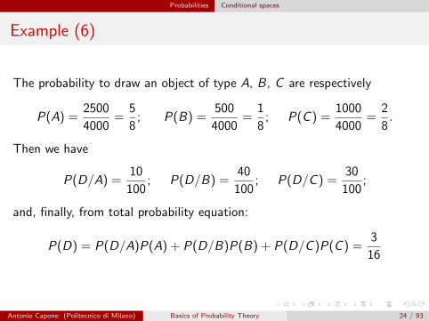
The probability to draw an object of type A, B, C are respectively

P(A) =2500

4000=

5

8; P(B) =

500

4000=

1

8; P(C ) =

1000

4000=

2

8.

Then we have

P(D/A) =10

100; P(D/B) =

40

100; P(D/C ) =

30

100;

and, finally, from total probability equation:

P(D) = P(D/A)P(A) + P(D/B)P(B) + P(D/C )P(C ) =3

16



Example (7)

A game is based on the following experiment. A box contains n tags, eachone reporting a number arbitrarily determined. The player draws at first rtags and observes their maximum value mr . Then, further drawings areperformed until a value m is observed such as m > Mr .

Player wins if m = M, where M is the maximum value among thosereported on the n tags. We want to evaluate the probability P(V ) to win.



Example (7)

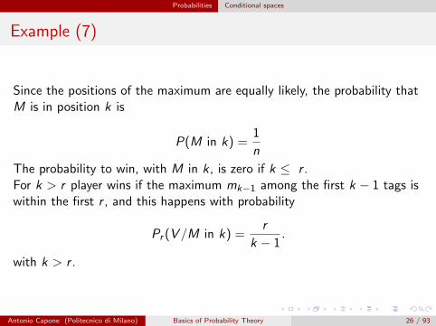
Since the positions of the maximum are equally likely, the probability thatM is in position k is

P(M in k) =1

n

The probability to win, with M in k , is zero if k ≤ r .For k > r player wins if the maximum mk−1 among the first k − 1 tags iswithin the first r , and this happens with probability

Pr (V /M in k) =r

k − 1.

with k > r .



Example (7)

By the Total Probability Theorem (11) we have:

Pr (V ) =n∑

k=1

Pr (V /M in k)P(M in k) =

=r∑

k=1

Pr (V /M in k)P(M in k) +n∑

k=r+1

Pr (V /M in k)P(M in k) =

=n∑

k=r+1

r

k − 1

1

n=

r

n

n−1∑k=r

1

k.


Probabilities Bayes’ Formulas

Bayes’ Formulas

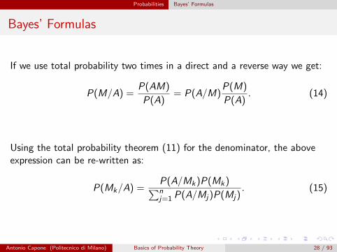
If we use total probability two times in a direct and a reverse way we get:

P(M/A) =P(AM)

P(A)= P(A/M)

P(M)

P(A). (14)

Using the total probability theorem (11) for the denominator, the aboveexpression can be re-written as:

P(Mk/A) =P(A/Mk)P(Mk)∑nj=1 P(A/Mj)P(Mj)

. (15)



Bayes’ Formulas

Bayes’ formulas are particularly useful for evaluating conditionalprobabilities before and after observing the occurrence of an event.

In particular, the second formula is referred to as ”Bayes’ rule for the’a posteriori’ probability”, that is after observing the occurrence ofthe event A.

In this case, P(Mi ) are called ”a priori probabilities” and P(Mi/A) ”aposteriori probabilities”.



Example (8)

An object drawn at random from the box in Example (6) is found to bedefective. Evaluate the probabilities that it is of type A, B and Crespectively.

Using Bayes’ formula and the preceding results we have

P(A/D) =P(D/A)P(A)

P(D)=

10

30; P(B/D) =

P(D/B)P(B)

P(D)=

8

30.

Similarly we have

P(C/D) =12

30.

Note that while ”a priori” the most likely type of object is A, afterobserving that the object is defective the most likely type of object is C .



Example (9)

Assume that you are presented with three dices, two of them fair and theother a counterfeit that always gives 6. If you randomly pick one of thethree dices, the probability that it’s the counterfeit is 1/3.

This is the a priori probability of the hypothesis that the dice iscounterfeit. Now after throwing the dice, you get 6 for two consecutivetimes. Seeing this new evidence, you want to calculate the revised aposteriori probability that it is the counterfeit.



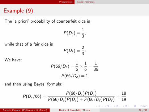
Example (9)

The ’a priori’ probability of counterfeit dice is

P(Dc) =1

3,

while that of a fair dice is

P(Df ) =2

3.

We have:

P(66/Df ) =1

6× 1

6=

1

36

P(66/Dc) = 1

and then using Bayes’ formula:

P(Dc/66) =P(66/Dc)P(Dc)

P(66/Dc)P(Dc) + P(66/Df )P(Df )=

18

19


Probabilities Statistical independence

Statistical independence

Two events A and B ⊂ S are said statistically independent if and only if

P(AB) = P(A)P(B) (16)

The meaning of statistical independence is immediate if we observe that ifA and B are independent:

P(A/B) = P(A), P(B/A) = P(B).

This means that the probability of A is not influenced by the occurrence ofB and vice versa.



Example (10)

In a throw of the dice, check whether the following eventsA = even numberB = number one, or two or threeare statistically independent.

We have

P(A) = 1/2; P(B) = 1/2; P(AB) = 1/6;

that isP(AB) 6= P(A)P(B)

Hence, events A e B are not statistically independent.



Example (11)

In a throw of the dice, check whether the following events A = an evennumber appearsB = number one, or two, or three, or four appearsare statistically independent.

We haveP(A) = 1/2; P(B) = 2/3; P(AB) = 2/6

andP(AB) = P(A)P(B)

Hence, events A e B are indeed statistically independent.


Random Variables

Random Variables




Random Variables Spaces with infinite outcomes

Spaces with countable outcomes

To deal with spaces S with infinite outcomes, we must add another axiomthat extends the summation of the probability measure over infinite terms:

Axiom IIIa: If A1,A2, . . . ,An . . . are disjoint events andA = A1 + A2 + . . .+ An + . . ., then

P(A) = P(A1) + P(A2) + . . .+ P(An) + . . . (17)

An example of this type of space is the number of coin flips to get a head.This number is not limited, as the head could never appear in n trial,whichever n is.These spaces are said countable (number of elements of the samecardinality of natural numbers), and can be managed with the methods offinite spaces.



Spaces with uncountable outcomes

We can consider also uncountable spaces, such as is the case whenthe outcomes is, for example, a point in an interval, or in any generalgeometrical space

The extension to these spaces is however not straightforward andrequire new instruments

The approach used is that of ”transforming” the space of outcomesinto another one more convenient for assigning probabilities.

In particular, we map outcomes and events (subsets) of S into thespace of real numbers (using integer numbers as a subset to includecountable spaces as a special case)



Definition of Random Variable

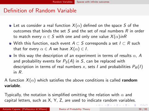
Let us consider a real function X (α) defined on the space S of theoutcomes that binds the set S and the set of real numbers R in orderto match every α ∈ S with one and only one value X (α)inR

With this function, each event A ⊂ S corresponds a set I ⊂ R suchthat for every α ∈ A we have X (α) ∈ I .

In this way the description of an experiment in terms of results α, Aand probability events for PS(A) in S , can be replaced withdescription in terms of real numbers x , sets I and probabilities PR(I )in R.

A function X (α) which satisfies the above conditions is called randomvariable.

Typically, the notation is simplified omitting the relation with α andcapital letters, such as X, Y, Z, are used to indicate random variables.



Cumulative Distribution Function (CDF)

Let X be a Random Variable (RV) and x a real number.The probability of the event {X ≤ x} is a function of the real variable x :

FX (x) = P(X ≤ x) (18)

and is called Cumulative Probability Distribution Function (CDF) of X .

FX (x) completely describes RV X .In fact we have, for any x1, x2 and x :

P(x1 < X ≤ x2) = F (x2)− F (x1) (19)

P(X = x) = F (x)− F (x−) (20)

We denote F (x+) = limε→0 and F (x−) = limε→0 F (x − ε)Antonio Capone (Politecnico di Milano) Basics of Probability Theory 40 / 93


Cumulative Distribution Function (CDF)

The CDF has the following properties:

1 it has the following limits

F (−∞) = 0 F (+∞) = 1 (21)

2 it is a monotonic non decreasing function of x :

F (x1) ≤ F (x2) per x1 ≤ x2 (22)

3 it is right continuous :F (x+) = F (x) (23)


Random Variables Continuous Random Variables

Continuous Random VariablesProbability Density Function (pdf)

A RV X is continuous if its CDF FX (x) is a continuous function inR, together with its first derivative, except at most a countable set ofpoints where the derivative does not exist.

Since for a continuous RV FX (x), we have

P(X = x) = 0.

It is therefore useful introducing the probability density function(pdf) of RV X , fX (x) defined as the derivative of the correspondingCDF:

fX (x) =dFX (x)

dx(24)

The definition is then completed by assigning arbitrary positive valueswhere the derivative does not exist.



Probability Density Function (pdf)

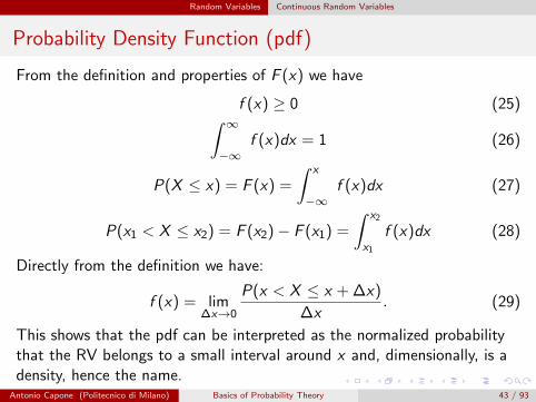
From the definition and properties of F (x) we have

f (x) ≥ 0 (25)∫ ∞−∞

f (x)dx = 1 (26)

P(X ≤ x) = F (x) =

∫ x

−∞f (x)dx (27)

P(x1 < X ≤ x2) = F (x2)− F (x1) =

∫ x2

x1

f (x)dx (28)

Directly from the definition we have:

f (x) = lim∆x→0

P(x < X ≤ x + ∆x)

∆x. (29)

This shows that the pdf can be interpreted as the normalized probabilitythat the RV belongs to a small interval around x and, dimensionally, is adensity, hence the name.



Example (12) - Uniform RV

We want to find the CDF and pdf of RV X , defined as the coordinate of apoint randomly selected in interval [a, b] of x axis.

We have

FX (x) =

x − a

b − a(a ≤ x ≤ b)

0 (x < a)1 (x > b)

(30)

and from definition (29):

f (x) = lim∆x→0

∆x

b − a

1

∆x



Example (12)

we get

fX (x) =

1

b − a(a ≤ x ≤ b)

0 elsewhere

(31)

1

a b x

FX(x)

a b x

fX(x)

ab −

1

A RV that satisfies (30) and (31) is called ”uniformly distributed” and thepdf is said ”uniform”.



Example (13)

A point P is drawn uniformly on a circumference of radius R and center inthe origin of axes. Find the pdf of RV X , defined as the coordinate oforthogonal projection of P on the horizontal axis.

xR-R

R

Ox x+dx

dl

dl

a b

fX(x)

To find the pdf let us use the definition (29). With reference to the figure,P(x < X ≤ x + ∆x) is the probability that P lies in one of two small arcsshown in the figure, each having a length

d` =√

dx2 + dy 2 = dx

√1 + (

dy

dx)2



Example (13)

Being y =√

R2 − x2, we get:

dy = − xdx√R2 − x2

by replacing it in the expression above we get

d` = dx

√1 +

x2(dx)2

R2 − x2

1

(dx)2=

dx√1− (

x

R)2

.



Example (13)

Then we have:

fX (x) = lim∆x→0

1

∆x

2∆l

2πR= lim

∆x→0

1

∆x

1

2πR

2∆x√1− (x/R)2

=

=1

πR

1√1− (x/R)2

for (| x |≤ R) and zero elsewhere.

xR-R

R

Ox x+dx

dl

dl

a b

fX(x)



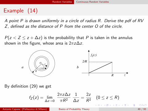
Example (14)

A point P is drawn uniformly in a circle of radius R. Derive the pdf of RVZ , defined as the distance of P from the center O of the circle.

P(z < Z ≤ z + ∆z) is the probability that P is taken in the annulusshown in the figure, whose area is 2πz∆z .

R

O z

z+dz

R z

fZ(z)

2/R

a b

By definition (29) we get

fZ (z) = lim∆z→0

2πz∆z

πR2

1

∆z=

2z

R2(0 ≤ z ≤ R)



Example (15) - Negative Exponential RV

The ”Negative Exponential” pdf is defined as:

F (x) = 1− e−λx (x ≥ 0) (32)

we have:f (x) = λe−λx (x ≥ 0) (33)

1

x

FX(x)

x

fX(x)λ

a b


Random Variables Discrete Random Variables

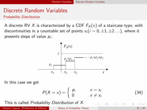
Discrete Random VariablesProbability Distribution

A discrete RV X is characterized by a CDF FX (x) of a staircase type, withdiscontinuities in a countable set of points xi (i = 0,±1,±2 . . .), where itpresents steps of value pi :

x

FX(x)

x3x2x1

1

p1

p1+p2p

1+p

2+p

3

In this case we get

P(X = x) =

{pi x = xi0 x 6= xi

(34)

This is called Probability Distribution of X .Antonio Capone (Politecnico di Milano) Basics of Probability Theory 51 / 93


Probability Distribution

For the Probability Distribution, we have

pi ≥ 0 (35)

∞∑i=−∞

pi = 1 (36)

F (x) =M∑

i=−∞pi (37)

where M is the maximum i for which xi ≤ x .If the values xi are integers, then RV X is said an integer RV.



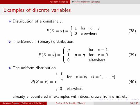
Examples of discrete variables

Distribution of a constant c:

P(X = x) =

{1 for x = c0 elsewhere

(38)

The Bernoulli (binary) distribution:

P(X = x) =

p for x = 11− p = q for x = 00 elsewhere

(39)

The uniform distribution

P(X = x) =

1

nfor x = xi (i = 1, . . . , n)

0 elsewhere

(40)

already encountered in examples with dices, draws from urns, etc.



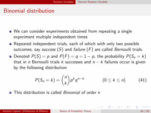
Binomial distribution

We can consider experiments obtained from repeating a singleexperiment multiple independent times

Repeated independent trials, each of which with only two possibleoutcomes, say success (S) and failure (F ) are called Bernoulli trials.

Denoted P(S) = p and P(F ) = q = 1− p, the probability P(Sn = k)that in n Bernoulli trials k successes and n − k failures occur is givenby the following distribution

P(Sn = k) =

(n

k

)pkqn−k (0 ≤ k ≤ n) (41)

This distribution is called Binomial of order n



Example (16)

A quality control process tests some components out of a factory andcomponents are found defective with a probability p = 10−2. Evaluate theprobability that out of 10 components checked there areA = only one defectiveB = two defectiveC = at least one defectiveThe 10 tests can be modeled as Bernoulli trials with success probabilityp = 1

100 . Then we have

P(A) = (101

)(1

100)1(

99

100)9 = 0, 0913 . . .

P(B) = (102

)(1

100)2(

99

100)8 = 0, 00415 . . .

P(C ) =10∑k=1

(10k

)(1

100)k(

99

100)10−k = 1−(

100

)(1

100)0(

99

100)10 = 0, 0956 . . .


Random Variables Moments of a pdf

Moments of a pdf

For the pdf we can define some parameters that resume some properties ofthe function. These are called moments, and the most used are:

1 k−th order moments (k = 1, 2, . . .)

mk =

∫ +∞

−∞xk f (x)dx (42)

2 k−th order central moments

µk =

∫ +∞

−∞(x −m1)k f (x)dx (43)

Note that, depending on the specific pdf, some moments may not exist.



Moments of a pdf

Parameters of the same meaning can be given also for discrete variables inthe form:

mk =∞∑

i=−∞xki pi (44)

µk

∞∑i=−∞

(xi −m1)k pi (45)



Moments of a pdf

The first order moment:

m1 =

∫ +∞

−∞x f (x)dx (also denoted mX )

This can be considered as the coordinate of the center of massinterpreting the pdf as a mass distribution along the x with densityf (x).

The index µ2:

µ2 =

∫ +∞

−∞(x −m1)2f (x)dx (also denoted σ2

X )

provides an index of the dispersion of the distribution around x = mX

we haveµ2 = m2 −m2

1



Law of large numbers

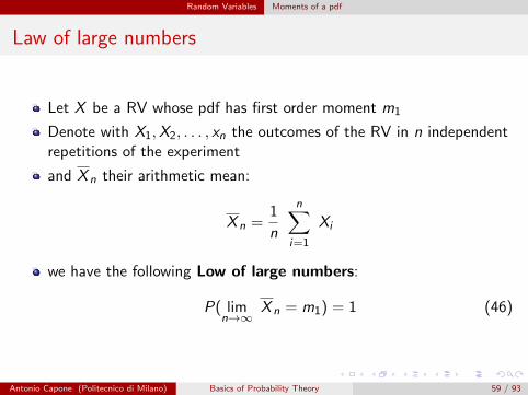
Let X be a RV whose pdf has first order moment m1

Denote with X1,X2, . . . , xn the outcomes of the RV in n independentrepetitions of the experiment

and X n their arithmetic mean:

X n =1

n

n∑i=1

Xi

we have the following Low of large numbers:

P( limn→∞

X n = m1) = 1 (46)



Law of large numbers

Law of large numbers states that the average performed on a numbern of outcomes of n independent trials, tends with probability 1 to m1

when n tends to infinity.

For this reason, m1 is also called the mean value or expected value ofRV X and it is also denoted by E [X ].

This law is of great importance since it provides a relationshipbetween a pure mathematical parameter, m1, to another one X n

directly derived from an experiment.



Interpretation of probability

Let’s formulate the law of large numbers for probability pA of event ADefine the binary RV X such that it is X = 1 if A occurs and X = 0otherwiseIf we perform n trials we have

n∑i=1

Xi = nA

being nA the number of times A occurswe also observe that

m1(X ) = pA

andX n =

nA

n.

Therefore, the law of large numbers can be written as

P( limn→∞

nA

n= pA) = 1 (47)

The above formulation of the law provides the interpretation ofprobability P(A) as the limit of frequencies nA/n.



Properties of E[X]

Some properties of E [X ] are (for proofs see lecture notes):1 If f (x) is symmetric around a value of a and m1 exists, then m1 = a2 If m1 exists, it can be expressed as

m1 =

∫ ∞0

(1− F (x))dx −∫ 0

−∞F (x)dx (48)

3 If FX (x) = 0 for x < 0, for α > 0 the following inequality holds

P(X ≥ α) ≤ E [X ]

α(49)

Setting v =α

E [X ]we get a different expression

P(X ≥ vE [X ]) ≤ 1

v(50)

that shows how to establish a constraint upon the part of pdf that liesabove the mean value (v > 1), based on the sole knowledge of themean value.



Tchebichev inequality

Central moment µ2, is also called variance of RV X and denoted byσ2X , whereas σX is called standard deviation

The variance represents a measure of the dispersion of f (x) around itsaverage value

This is shown by the Tchebichev Inequality

P(| X −m1 | ≥ vσ) <1

v 2(51)

By setting vσ = ε we get alternatively

P(m1 − ε < X < m1 + ε) ≥ 1− σ2

ε2(52)

P(|X −m1| ≥ ε) ≤ σ2

ε2(53)



Example (17)

Let us apply Tchebichev inequality to bound the probability that thefrequency of HEADS in flipping a fair coin n times exceeds 0.5± ε.

The frequency of HEADS in n trials is H/n where H is the RV number ofHEADS in n trials. This has a Binomial distribution with average n/2 andσ2(H) = n/4. Therefore,

m1(H/n) =1

2

σ2(H/n) =1

4nTchebichev inequality says

P(|H/n −m1| ≥ ε) ≤ σ2

ε2

and substituting

P(|H/n − 0.5| ≥ ε) ≤ 1

4nε2



Example (17)

we have

ε = 0.1, n = 10, P ≤ 2.5(???)

ε = 0.1, n = 100, P ≤ 0.25

ε = 0.1, n = 1000, P ≤ 0.025

ε = 0.1, n = 10000, P ≤ 0.0025

We also see that

limn→∞

P(|H/n − 0.5| ≥ ε) = 0, ∀ε > 0

that provides a kind of demonstration of the law of large numbers.


Random Variables Conditional distributions and densities

Conditional distributions and densities

Let M be an event of space S where RV X is defined. We define CDF ofX conditional to M (provided that P(M) 6= 0) the function:

FX (x/M) = P(X ≤ x/M) (54)

and similarly for the density a

fX (x/M) =dFX (x/M)

dx= lim

∆x→0

P(x < X ≤ x + ∆x/M)

∆x(55)

It is easy to check that the above defined functions have all the propertiesof the CDF and pdf.



Conditional distributions and densities

Interesting cases are those where also event M is described in terms of RVX .We define probability of an event A conditional to the value x assumed bya RV X , assuming that fX (x) 6= 0, as the limit

P(A/X = x) = lim∆x→0

P(A/x < X ≤ x + ∆x) (56)

From Bayes formula (14) we get:

P(A/X = x) = lim∆x→0

P(x < X ≤ x + ∆x/A)P(A)

P(x < X ≤ x + ∆x)

and multiplying by ∆x above and below, and taking the limit, we havefinally

P(A/X = x) =fX (x/A)P(A)

fX (x)(57)



Total probability law for the continuous case

From (57) we have by integrating left and right sides:∫ +∞

−∞fX (x/A)P(A)dx =

∫ +∞

−∞P(A/X = x)fX (x)dx

and, by observing that

∫ +∞

−∞fX (x/A)dx = 1, we have

P(A) =

∫ +∞

−∞P(A/X = x)fX (x)dx (58)

This is the Total probability law for the continuous case.



Bayes’ formula for the continuous case

Furthermore from (57), and using (58), we obtain:

fX (x/A) =P(A/X = x)fX (x)

P(A)=

P(A/X = x)fX (x)∫ +∞

−∞P(A/X = x)fX (x)dx

(59)

which represents the Bayes theorem extended to the continuous. case.



Example (18)

Four points A,B,C and D are chosen uniformly and independently on acircumference. Find the probability of eventI = {intersection of chords AB and CD}.

Denoted by L the length of the circumference and by x the RV length ofarc AB(oriented), and assumed X = x , we have

P(I/X = x) = P(D ∈ AB)P(C ∈ BA) + P(D ∈ BA)P(C ∈ AB) =

= 2x(L− x)

L2

.

.

.

.

A

D

B

C



Example (18)

From total probability law, and being

fX (x) =1

L, (0 < x < L),

we get

P(I ) =

∫ L

0P(I/X = x)fX (x)dx =

∫ L

02

x(L− x)

L3dx =

1

3

The result can be found also observing that, once A is taken, thesequences derived from the permutations of the other 3 points are equallylikely, and among these only two lead to a chord intersection.


Random Variables Vectorial Random Variables

Multiple Random Variables

We can extend definitions of a scalar RV (defined on real numbers R)to the case of multiple RV’s defined on multidimensional spaces

We focus on the case of two RVs, being the extension to more thantwo RVs straightforward

Consider two RV X (α) and Y (α) defined in the same result space S

We have a correspondence between each event A ⊂ S and a set Dxy

of the Cartesian plane, such that for every α ∈ A the point withcoordinates X (α) and Y (α) belongs to Dxy .

Thus, a joint event in S is represented by a domain Dxy in theCartesian plane.



Joint CDF

The probability of the joint events {X ≤ x ,Y ≤ y} = {X ≤ x}{Y ≤ y} isa function of the pair of real variables x and y :

FXY (x , y) = P(X ≤ x ,Y ≤ y) (60)

Such a function is called joint CDF of RVs X and Y .

y

x

(x,y) y2

x2

y1

x1

a b



Joint CDF

From the definition we can easily verify the following relations:

F (x ,∞) = FX (x); F (∞, y) = FY (y) (61)

F (∞,∞) = 1 (62)

F (x ,−∞) = 0; F (−∞, y) = 0 (63)

P(x1 < X ≤ x2, y1 < Y ≤ y2) = F (x2, y2)−F (x1, y2)−F (x2, y1)+F (x1, y1)(64)

y

x

(x,y) y2

x2

y1

x1

a b



Joint pdf

Assuming now that FXY (x , y) is derivable, the joint pdf of RVs X and Y is

fXY (x , y) =∂2F (x , y)

∂x∂y(65)

The properties holdf (x , y) ≥ 0 (66)∫ ∞

−∞

∫ ∞−∞

f (x , y)dxdy = 1 (67)

Furthermore, from the definition of the joint derivative we have

f (x , y) = lim∆x ,∆y→0

P(x < X < x + ∆x , y < Y < y + ∆y)

∆x∆y(68)



Joint pdf

The event including all results where X (α) and Y (α) belong to a domainD can be written as a union or intersection of elementary events of thetype

{x < X ≤ x + ∆x , y < Y ≤ y + ∆y}

and, therefore, we have

P((X ,Y ) ∈ D) =

∫ ∫D

f (x , y)dxdy (69)

where the integral is extended over the domain D.It also follows that

fX (x) =

∫ ∞−∞

f (x , y)dy ; fY (y) =

∫ ∞−∞

f (x , y)dx (70)

When dealing with multiple RVs, the pdf of each RV is called marginal.



Example (19)

Find the joint and marginal pdf of RV’s X and Y Cartesian coordinates ofa point Q chosen uniformly in a

a) square of side L and centered at the origin

b) circle of radius R and center at the origin

y

x

L/2-L/2

y

xR

a b



Example (19)

To find the joint density we use definition (68).In this expression the probability at the numerator the probability Q liesinto the rectangle of coordinates x , x + ∆x , y , y + ∆y , but since Q is

picked uniformly, this probability has value∆x∆y

S, S being the area of the

domain, regardless of the location of the small rectangle. Therefore, weobtain

f (x , y) =

1

Sfor(x , y) ∈ S

0 elsewhere

(71)

Such a pdf is still called Uniform in S and the value of the constant 1/Sdepends only from the area of the domain and not by its shape.



Example (19)

About the marginal pdf we havea)

fX (x) =

∫ +∞

−∞f (x , y)dy =

∫ L2

− L2

1

L2dy =

1

L;

(−L

2< x <

L

2

)and similarly

fY (y) =1

L;

(−L

2< y <

L

2

)In this case, the marginal pdf are uniform.b)

fX (x) =

∫ +∞

−∞f (x , y)dy =

∫ √R2−x2

−√R2−x2

1

πR2dy =

2

πR2

√R2 − x2; (| x |< R)

Here, the marginal pdf’s are no longer uniform. In fact, the shape of thedomain of point (X ,Y ) influences the result.



Conditional pdf

• pdf of RV Y conditioned by the value assumed by another RV X

fY (y/X = x) =fXY (x , y)

fX (x)(72)

• Total Probability Theorem

fY (y) =

∫ +∞

−∞fY (y/X = x)fX (x)dx (73)

• Bayes’ Theorem

fY (y/X = x) =fX (x/Y = y)fY (y)

fX (x)(74)



Conditional pdf

• Conditional mean

E [Y /X = x ] =

∫ +∞

−∞yfY (y/X = x) (75)

• Total Probability Theorem with respect to the mean

E [Y ] =

∫ +∞

−∞E [Y /x ]fX (x)dx (76)



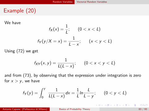
Example (20)

A point of coordinate X is uniformly selected within interval [0; L] of xaxis; Another point of coordinate Y is uniformly selected within interval[X ; L]. Find the joint pdf of X ,Y , the marginal pdf of Y and theprobability P that the three segments of length X , Y , and Y − X canform a triangle.

x

y

L

L

L/2

y

x1

baD



Example (20)

We have

fX (x) =1

L; (0 < x < L)

fY (y/X = x) =1

L− x; (x < y < L)

Using (72) we get

fXY (x , y) =1

L(L− x); (0 < x < y < L)

and from (73), by observing that the expression under integration is zerofor x > y , we have

fY (y) =

∫ y

0

1

L(L− x)dx =

1

Lln

L

L− y; (0 < y < L)



Example (20)

The domain D, where X and Y are such as to allow the construction ofthe triangle, is shown in the figure

x

y

L

L

L/2

y

x1

baD

and we thus have

p =

∫ L2

0dx

∫ x+ L2

L2

1

L(L− x)dy = ln2− 1

2= 0, 1931 . . .



Statistically independent RVs

Two RV X and Y are said to be statistically independent if events{X ≤ x} e {Y ≤ y} are statistically independent for each x and y .It follows then that two random RV are independent if one of the followingrelations holds

FXY (x , y) = FX (x)FY (y)

fXY (x , y) = fX (x)fY (y)

fX (x/Y = y) = fX (x)

fY (y/X = x) = fY (y)



Example (21)

Given two RV’s X and Y independent and exponentially distributed withthe same average 1/λ, find:

a) the probability of the event {Y > αX} with α real positive;

b) the pdf fY (y/Y > αX ).

a) We could use the (69), being D the domain in which y > αx , and giventhe independence we have

fXY (x , y) = fX (x)fY (y) = λ2e−λ(x+y) (x , y > 0)

More immediately we can use the Total Probability Theorem

P(Y > αX ) =

∫ ∞0

P(Y > αX/X = x)fX (x)dx =

∫ ∞0

e−λαx λe−λxdx =

=1

α + 1

∫ ∞0

λ(α + 1)e−λ(α+1)xdx =1

(α + 1)



Example (21)

b) From the definition of conditional pdf, and from the result of point a)we get:

fY (y/Y > αX ) = lim∆y→0

1

∆y

P(y < Y ≤ y + ∆y ,Y > αX )

P(Y > αX )=

= lim∆y→0

1

∆y

P(y < Y ≤ y + ∆y ,X < y/α)

P(Y > αX )=

=

∫ y/α

0fXY (x , y)dx

P(Y > αX )=

λe−λy∫ y/α

0λe−λxdx

1/(α + 1)=

= (α + 1)λe−λy (1− e−λy/α) (y > 0)



Joint Moments

Given two RV’s X and Y the joint moments of order h and k are definedas

mhk =

∫ ∫xhyk fxy (x , y)dxdy

and the central moments of order h and k

µhk =

∫ ∫(x −mx)h(y −my )k fxy (x , y)dxdy .

The mixed second-order central moment µ11, said also Covariance of RVsX and Y , is of particular interest. It is linked to m11 by the followingrelation

µ11 = m11 −m10m01 (77)


Random Variables Functions of Random Variables

The sum of two continuous RV’s

Given the two continuous RV’s X e Y , whose joint pdf is known, we wantto find the pdf of their sum

Z = X + Y (78)

To this purpose, we note that

fZ (z/X = x) = fY (z − x/X = x) (79)

From the total probability theorem we have

fZ (z) =

∫fZ (z/X = x)fX (x)dx =

∫fY (z − x/X = x)fX (x)dx (80)

which provides the final formula

fZ (z) =

∫fXY (x , z − x)dx (81)

Symmetrically we have

fZ (z) =

∫fXY (z − y , y)dy (82)



The sum of two continuous RV’s

If X and Y are statistically independent the two above become

fZ (z) =

∫fX (x)fY (z − x)dx

fZ (z) =

∫fX (z − y)fY (y)dy

The operations above are known as the convolution of pdf’s.In fact, the convolution of functions f (x) and g(y) (need not to be pdf’s)is defined as

f (z) ∗ g(z) =

∫f (x)g(z − x)dx =

∫f (z − x)g(x)dx



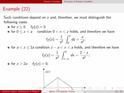
Example (22)

Find the pdf of RV Z = X + Y where X and Y are independent RVs withthe same pdf, namely

a) f (x) =1

a(0 < x < a)

b) f (x) = λe−λx (x > 0)

a) The integrating function in (90) is different from zero when both thefollowing conditions apply: {

0 < x < a0 < z − x < a

or {0 < x < az − a < x < z



Example (22)

Such conditions depend on z and, therefore, we must distinguish thefollowing cases:

for z ≤ 0 fZ (z) = 0for 0 ≤ z < a condition 0 < x < z holds, and therefore we have

fZ (z) =1

a2

∫ z

0dz =

z

a2;

for a < z ≤ 2a condition z − a < x < a holds, and therefore we have

fZ (z) =1

a2

∫ a

z−adx =

2− z

a2;

for z > 2a fZ (z) = 0;

fZ(z)

za 2aAntonio Capone (Politecnico di Milano) Basics of Probability Theory 92 / 93


Example (22)

b) The integrating function in (90) is different from zero when{x > 0z − x > 0

that is

{x > 0x < z

and, therefore, we have

fZ (z) =

∫ z

0λe−λxλe−λ(z−x)dx = λ2ze−λz (z > 0)


basics of probability theory - intranet...

Documents