basics of parallel systems and programs - sccswiki · pdf filebasics of parallel systems and...
TRANSCRIPT
Technische Universität München
Basics of Parallel Systemsand Programs
9th SimLab Course on Parallel Numerical Simulation
October 3—9, 2010, Belgrade, Serbia
Ralf-Peter Mundani
Technische Universität München
Technische Universität München
R.-P. Mundani - 9th SimLab Course on Parallel Numerical Simulation - October 3-9, 2010, Belgrade, Serbia 2
Overview
hardware aspects
supercomputers
network topologies
terms and definitions
Supercomputer: Turns CPU-bound problems into I/O-bound problems.
—Ken Batcher
Technische Universität München
R.-P. Mundani - 9th SimLab Course on Parallel Numerical Simulation - October 3-9, 2010, Belgrade, Serbia 3
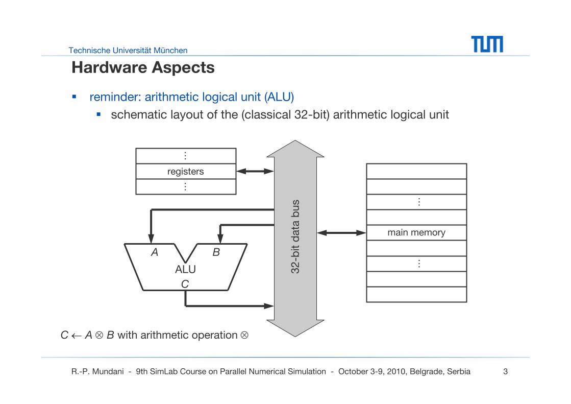
Hardware Aspects
reminder: arithmetic logical unit (ALU)
schematic layout of the (classical 32-bit) arithmetic logical unit
A B
C
ALU
registers
main memory
32-b
it d
ata
bus
……
……
C ← A ⊗ B with arithmetic operation ⊗
Technische Universität München
R.-P. Mundani - 9th SimLab Course on Parallel Numerical Simulation - October 3-9, 2010, Belgrade, Serbia 4
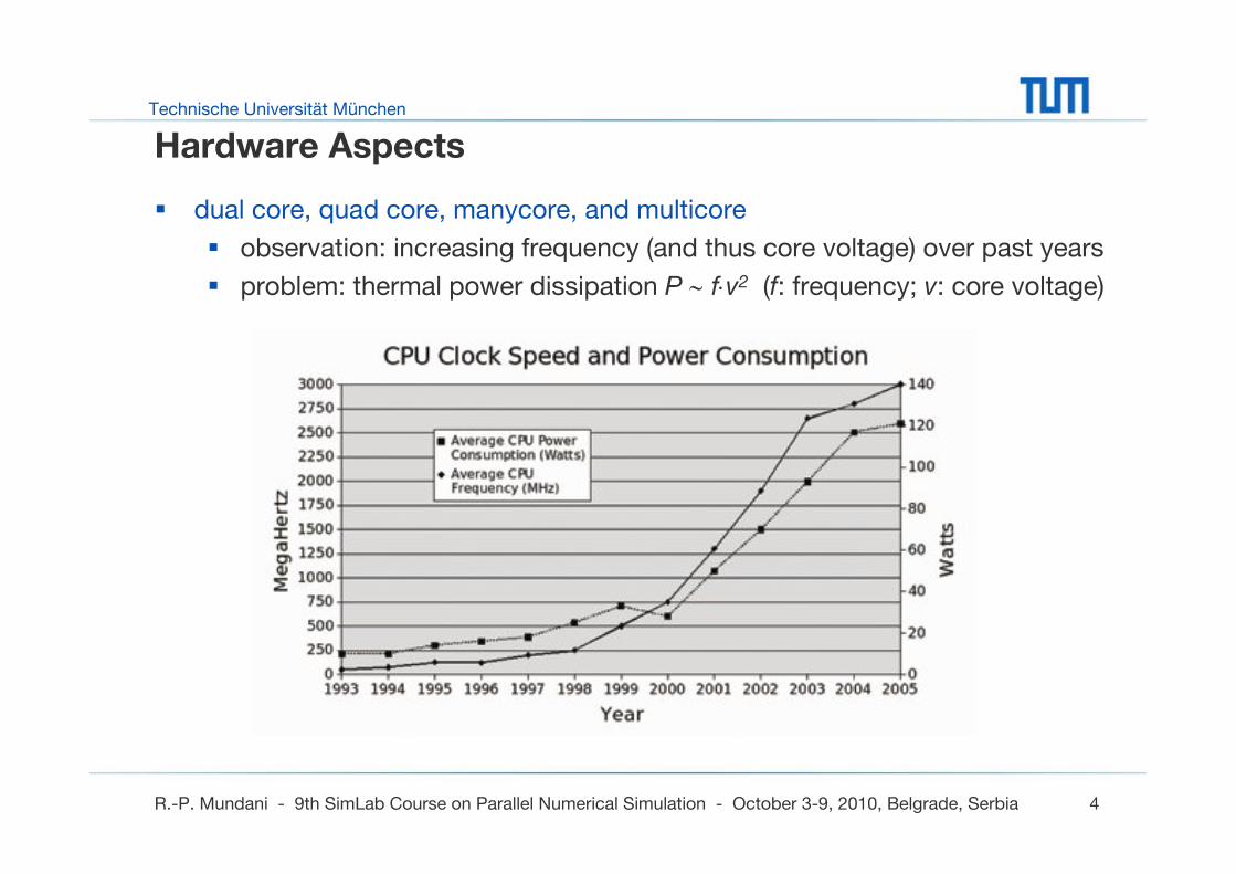
Hardware Aspects
dual core, quad core, manycore, and multicore
observation: increasing frequency (and thus core voltage) over past years
problem: thermal power dissipation P ∼ f⋅v2 (f: frequency; v: core voltage)
Technische Universität München
R.-P. Mundani - 9th SimLab Course on Parallel Numerical Simulation - October 3-9, 2010, Belgrade, Serbia 5
Hardware Aspects
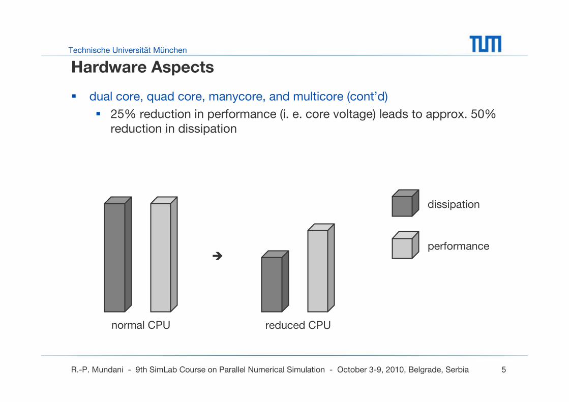
dual core, quad core, manycore, and multicore (cont’d)
25% reduction in performance (i. e. core voltage) leads to approx. 50% reduction in dissipation
dissipation
performance
normal CPU reduced CPU
Technische Universität München
R.-P. Mundani - 9th SimLab Course on Parallel Numerical Simulation - October 3-9, 2010, Belgrade, Serbia 6
Hardware Aspects
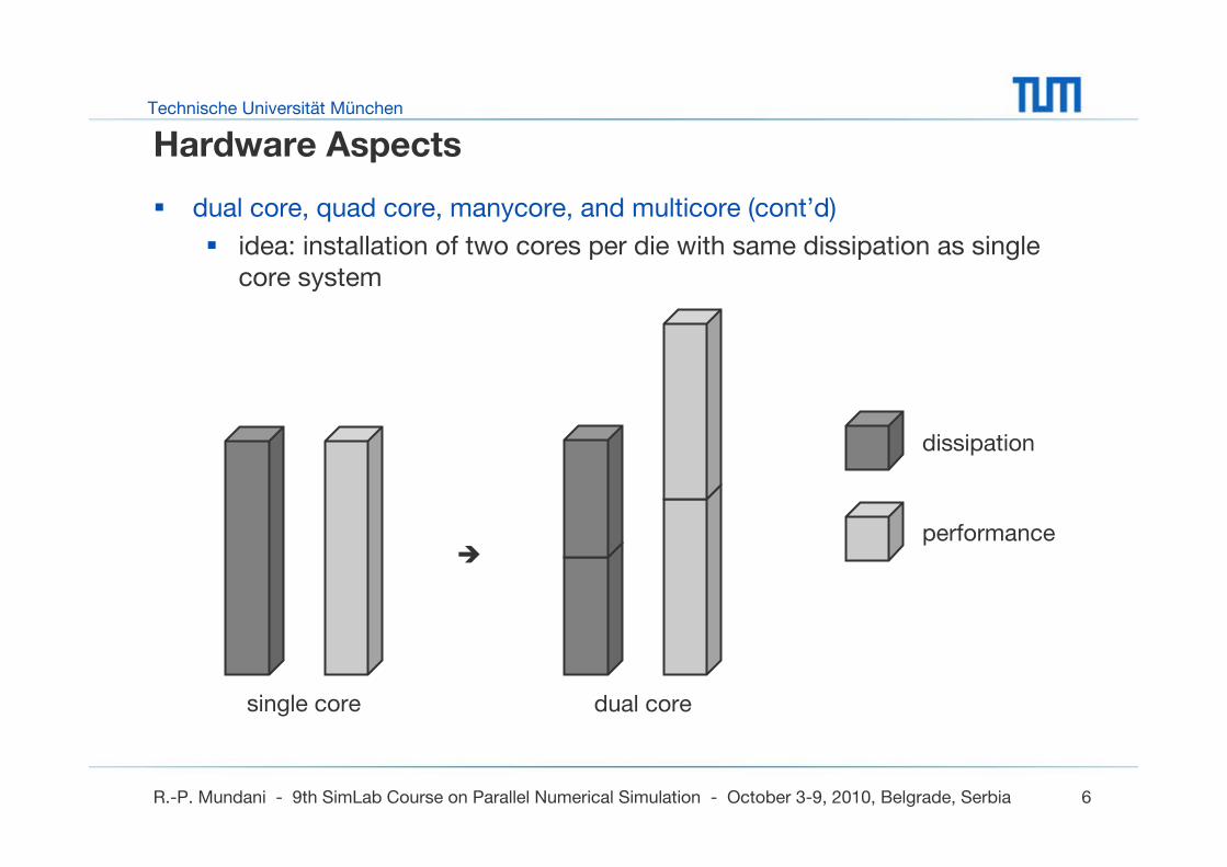
dual core, quad core, manycore, and multicore (cont’d)
idea: installation of two cores per die with same dissipation as single core system
dissipation
performance
single core dual core
Technische Universität München
R.-P. Mundani - 9th SimLab Course on Parallel Numerical Simulation - October 3-9, 2010, Belgrade, Serbia 7
Hardware Aspects
dual core, quad core, manycore, and multicore (cont’d)
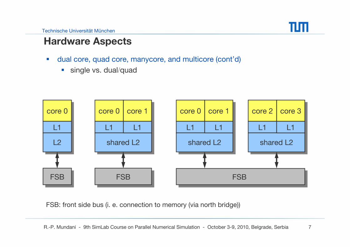
single vs. dual/quad
FSB
core 0
L1
L2
FSB
core 0 core 1
L1 L1
shared L2
FSB
core 0 core 1
L1 L1
shared L2
core 2 core 3
L1 L1
shared L2
FSB: front side bus (i. e. connection to memory (via north bridge))
Technische Universität München
R.-P. Mundani - 9th SimLab Course on Parallel Numerical Simulation - October 3-9, 2010, Belgrade, Serbia 8
Hardware Aspects
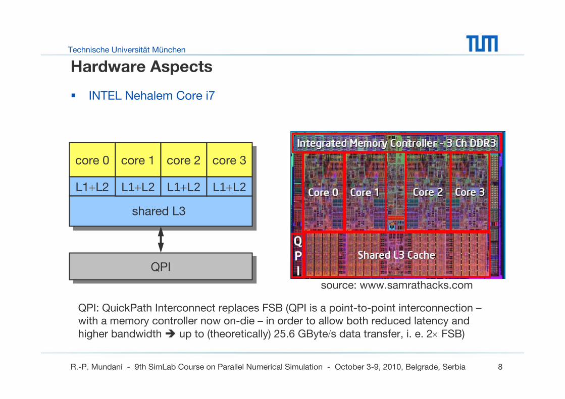
INTEL Nehalem Core i7
source: www.samrathacks.com
QPI
core 0 core 1
L1+L2 L1+L2
shared L3
core 2 core 3
L1+L2 L1+L2
QPI: QuickPath Interconnect replaces FSB (QPI is a point-to-point interconnection –with a memory controller now on-die – in order to allow both reduced latency and higher bandwidth up to (theoretically) 25.6 GByte/s data transfer, i. e. 2× FSB)
Technische Universität München
R.-P. Mundani - 9th SimLab Course on Parallel Numerical Simulation - October 3-9, 2010, Belgrade, Serbia 9
Hardware Aspects
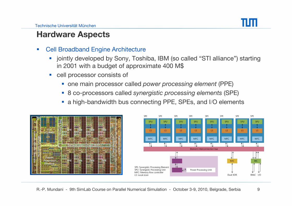
Cell Broadband Engine Architecture
jointly developed by Sony, Toshiba, IBM (so called “STI alliance”) starting in 2001 with a budget of approximate 400 M$
cell processor consists of
one main processor called power processing element (PPE)
8 co-processors called synergistic processing elements (SPE)
a high-bandwidth bus connecting PPE, SPEs, and I/O elements
Technische Universität München
R.-P. Mundani - 9th SimLab Course on Parallel Numerical Simulation - October 3-9, 2010, Belgrade, Serbia 10
Hardware Aspects
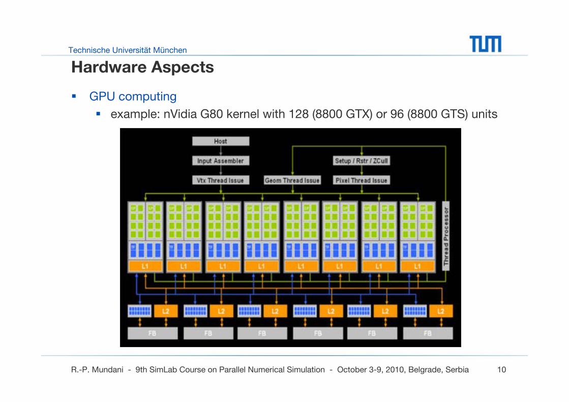
GPU computing
example: nVidia G80 kernel with 128 (8800 GTX) or 96 (8800 GTS) units
Technische Universität München
R.-P. Mundani - 9th SimLab Course on Parallel Numerical Simulation - October 3-9, 2010, Belgrade, Serbia 11
Hardware Aspects
dawning of manycore and multicore
strong aspects
shared memory simple parallelisation
increasing number of cores (> 100 proposed by INTEL)
also other HW available: GPU, e. g.
…
weak aspects
parallelisation necessary (TANSTAFL!)
memory limitations (parallel read/write access)
race conditions (algorithm dependent)
limited scalability
Technische Universität München
R.-P. Mundani - 9th SimLab Course on Parallel Numerical Simulation - October 3-9, 2010, Belgrade, Serbia 12
Overview
motivation
supercomputers
network topologies
terms and definitions
Technische Universität München
R.-P. Mundani - 9th SimLab Course on Parallel Numerical Simulation - October 3-9, 2010, Belgrade, Serbia 13
Supercomputers
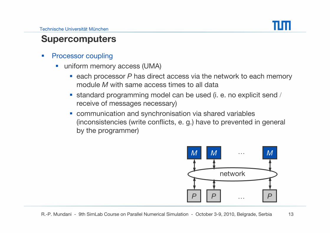
Processor coupling
uniform memory access (UMA)
each processor P has direct access via the network to each memory module M with same access times to all data
standard programming model can be used (i. e. no explicit send /receive of messages necessary)
communication and synchronisation via shared variables (inconsistencies (write conflicts, e. g.) have to prevented in general by the programmer)
M …
…
network
P PP
M M
Technische Universität München
R.-P. Mundani - 9th SimLab Course on Parallel Numerical Simulation - October 3-9, 2010, Belgrade, Serbia 14
Supercomputers
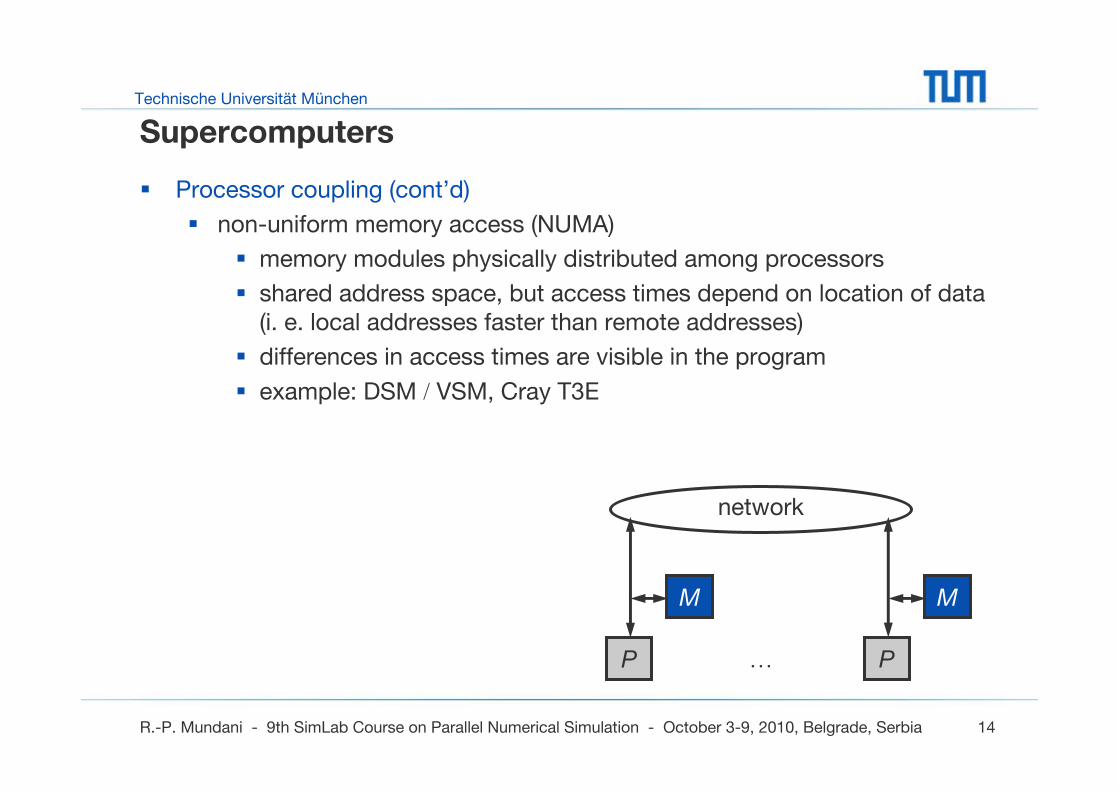
Processor coupling (cont’d)
non-uniform memory access (NUMA)
memory modules physically distributed among processors
shared address space, but access times depend on location of data (i. e. local addresses faster than remote addresses)
differences in access times are visible in the program
example: DSM / VSM, Cray T3E
P
M
…
network
M
P
Technische Universität München
R.-P. Mundani - 9th SimLab Course on Parallel Numerical Simulation - October 3-9, 2010, Belgrade, Serbia 15
Supercomputers
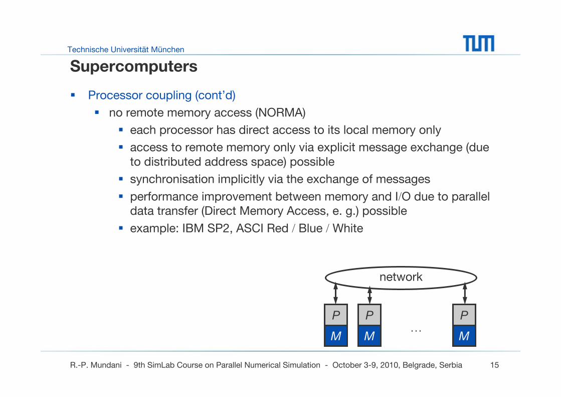
Processor coupling (cont’d)
no remote memory access (NORMA)
each processor has direct access to its local memory only
access to remote memory only via explicit message exchange (due to distributed address space) possible
synchronisation implicitly via the exchange of messages
performance improvement between memory and I/O due to parallel data transfer (Direct Memory Access, e. g.) possible
example: IBM SP2, ASCI Red / Blue / White
M
P…
network
M
P
M
P
Technische Universität München
R.-P. Mundani - 9th SimLab Course on Parallel Numerical Simulation - October 3-9, 2010, Belgrade, Serbia 16
Supercomputers
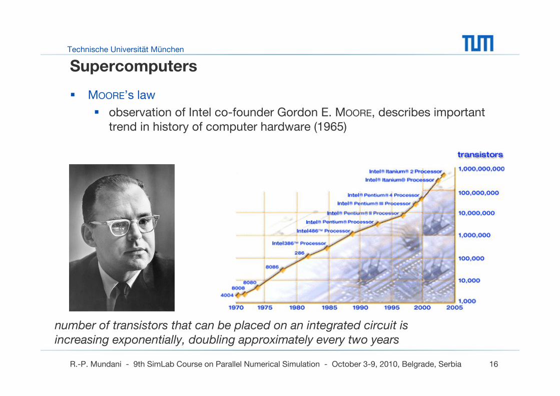
MOORE’s law
observation of Intel co-founder Gordon E. MOORE, describes important trend in history of computer hardware (1965)
number of transistors that can be placed on an integrated circuit is increasing exponentially, doubling approximately every two years
Technische Universität München
R.-P. Mundani - 9th SimLab Course on Parallel Numerical Simulation - October 3-9, 2010, Belgrade, Serbia 17
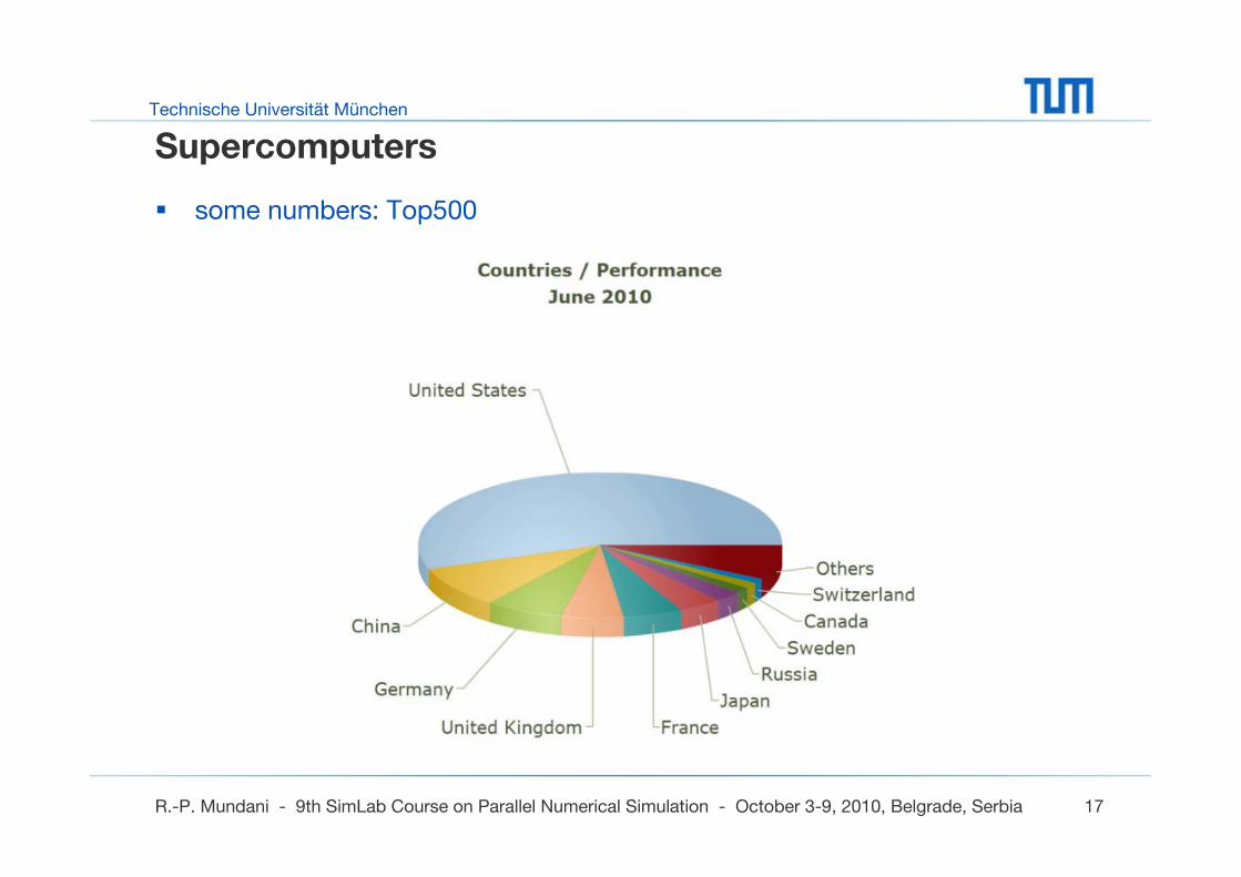
Supercomputers
some numbers: Top500
Technische Universität München
R.-P. Mundani - 9th SimLab Course on Parallel Numerical Simulation - October 3-9, 2010, Belgrade, Serbia 18
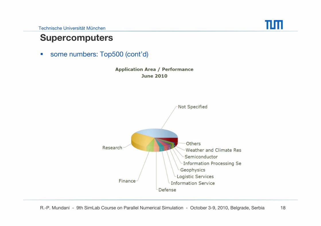
Supercomputers
some numbers: Top500 (cont’d)
Technische Universität München
R.-P. Mundani - 9th SimLab Course on Parallel Numerical Simulation - October 3-9, 2010, Belgrade, Serbia 19
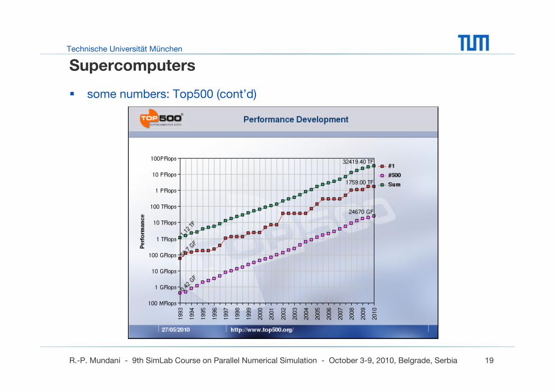
Supercomputers
some numbers: Top500 (cont’d)
Technische Universität München
R.-P. Mundani - 9th SimLab Course on Parallel Numerical Simulation - October 3-9, 2010, Belgrade, Serbia 20
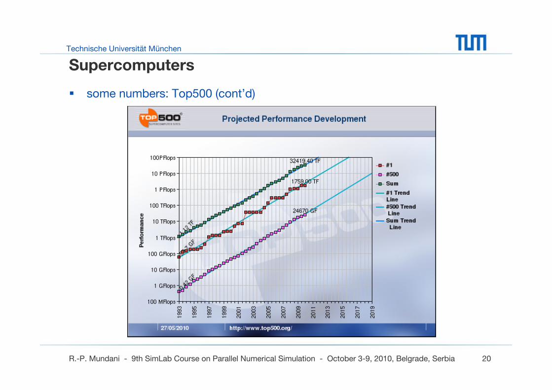
Supercomputers
some numbers: Top500 (cont’d)
Technische Universität München
R.-P. Mundani - 9th SimLab Course on Parallel Numerical Simulation - October 3-9, 2010, Belgrade, Serbia 21
Supercomputers
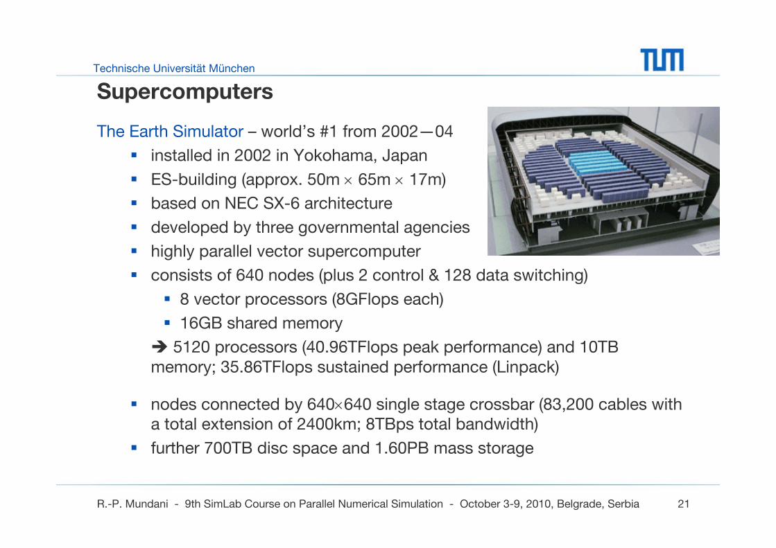
The Earth Simulator – world’s #1 from 2002—04
installed in 2002 in Yokohama, Japan
ES-building (approx. 50m × 65m × 17m)
based on NEC SX-6 architecture
developed by three governmental agencies
highly parallel vector supercomputer
consists of 640 nodes (plus 2 control & 128 data switching)
8 vector processors (8GFlops each)
16GB shared memory
5120 processors (40.96TFlops peak performance) and 10TB memory; 35.86TFlops sustained performance (Linpack)
nodes connected by 640×640 single stage crossbar (83,200 cables with a total extension of 2400km; 8TBps total bandwidth)
further 700TB disc space and 1.60PB mass storage
Technische Universität München
R.-P. Mundani - 9th SimLab Course on Parallel Numerical Simulation - October 3-9, 2010, Belgrade, Serbia 22
Supercomputers
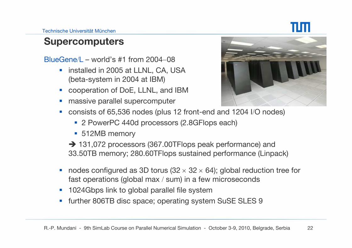
BlueGene/L – world’s #1 from 2004−08
installed in 2005 at LLNL, CA, USA(beta-system in 2004 at IBM)
cooperation of DoE, LLNL, and IBM
massive parallel supercomputer
consists of 65,536 nodes (plus 12 front-end and 1204 I/O nodes)
2 PowerPC 440d processors (2.8GFlops each)
512MB memory
131,072 processors (367.00TFlops peak performance) and33.50TB memory; 280.60TFlops sustained performance (Linpack)
nodes configured as 3D torus (32 × 32 × 64); global reduction tree for fast operations (global max / sum) in a few microseconds
1024Gbps link to global parallel file system
further 806TB disc space; operating system SuSE SLES 9
Technische Universität München
R.-P. Mundani - 9th SimLab Course on Parallel Numerical Simulation - October 3-9, 2010, Belgrade, Serbia 23
Supercomputers
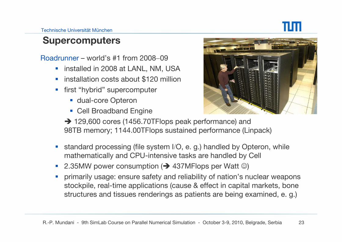
Roadrunner – world’s #1 from 2008−09
installed in 2008 at LANL, NM, USA
installation costs about $120 million
first “hybrid” supercomputer
dual-core Opteron
Cell Broadband Engine
129,600 cores (1456.70TFlops peak performance) and98TB memory; 1144.00TFlops sustained performance (Linpack)
standard processing (file system I/O, e. g.) handled by Opteron, while mathematically and CPU-intensive tasks are handled by Cell
2.35MW power consumption ( 437MFlops per Watt ☺)
primarily usage: ensure safety and reliability of nation’s nuclear weapons stockpile, real-time applications (cause & effect in capital markets, bone structures and tissues renderings as patients are being examined, e. g.)
Technische Universität München
R.-P. Mundani - 9th SimLab Course on Parallel Numerical Simulation - October 3-9, 2010, Belgrade, Serbia 24
Supercomputers
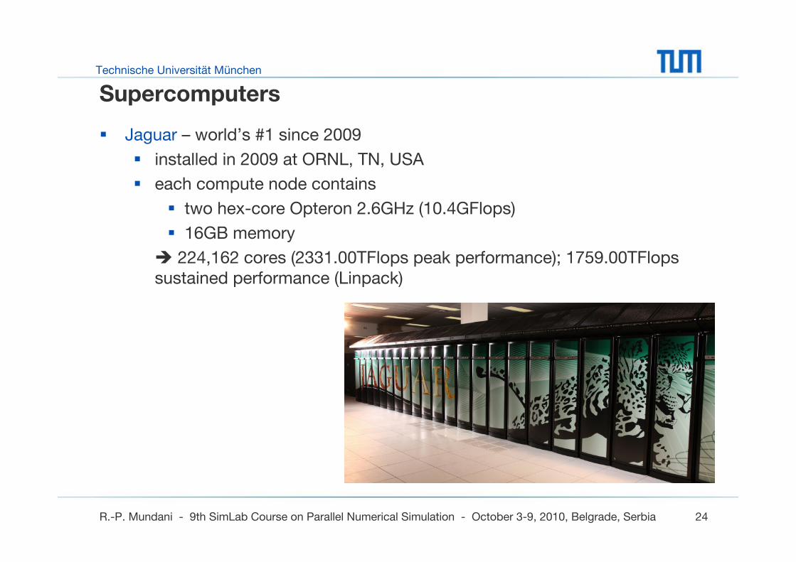
Jaguar – world’s #1 since 2009
installed in 2009 at ORNL, TN, USA
each compute node contains
two hex-core Opteron 2.6GHz (10.4GFlops)
16GB memory
224,162 cores (2331.00TFlops peak performance); 1759.00TFlops sustained performance (Linpack)
Technische Universität München
R.-P. Mundani - 9th SimLab Course on Parallel Numerical Simulation - October 3-9, 2010, Belgrade, Serbia 25
Overview
motivation
supercomputers
network topologies
terms and definitions
Technische Universität München
R.-P. Mundani - 9th SimLab Course on Parallel Numerical Simulation - October 3-9, 2010, Belgrade, Serbia 26
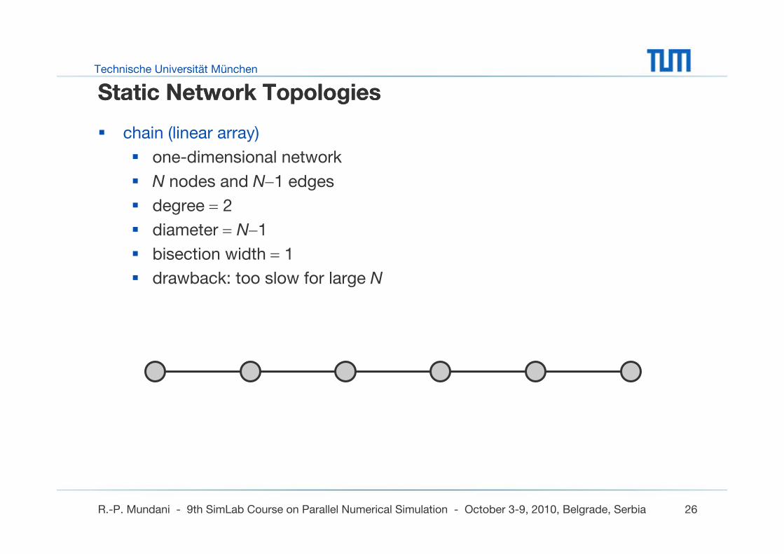
Static Network Topologies
chain (linear array)
one-dimensional network
N nodes and N−1 edges
degree = 2
diameter = N−1
bisection width = 1
drawback: too slow for large N
Static Network Topologies
Technische Universität München
R.-P. Mundani - 9th SimLab Course on Parallel Numerical Simulation - October 3-9, 2010, Belgrade, Serbia 27
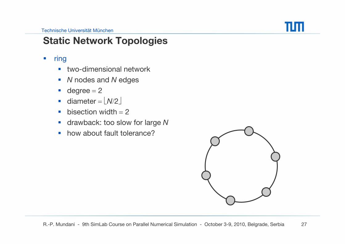
Static Network Topologies
ring
two-dimensional network
N nodes and N edges
degree = 2
diameter = ⎣N/2⎦bisection width = 2
drawback: too slow for large N
how about fault tolerance?
Technische Universität München
R.-P. Mundani - 9th SimLab Course on Parallel Numerical Simulation - October 3-9, 2010, Belgrade, Serbia 28
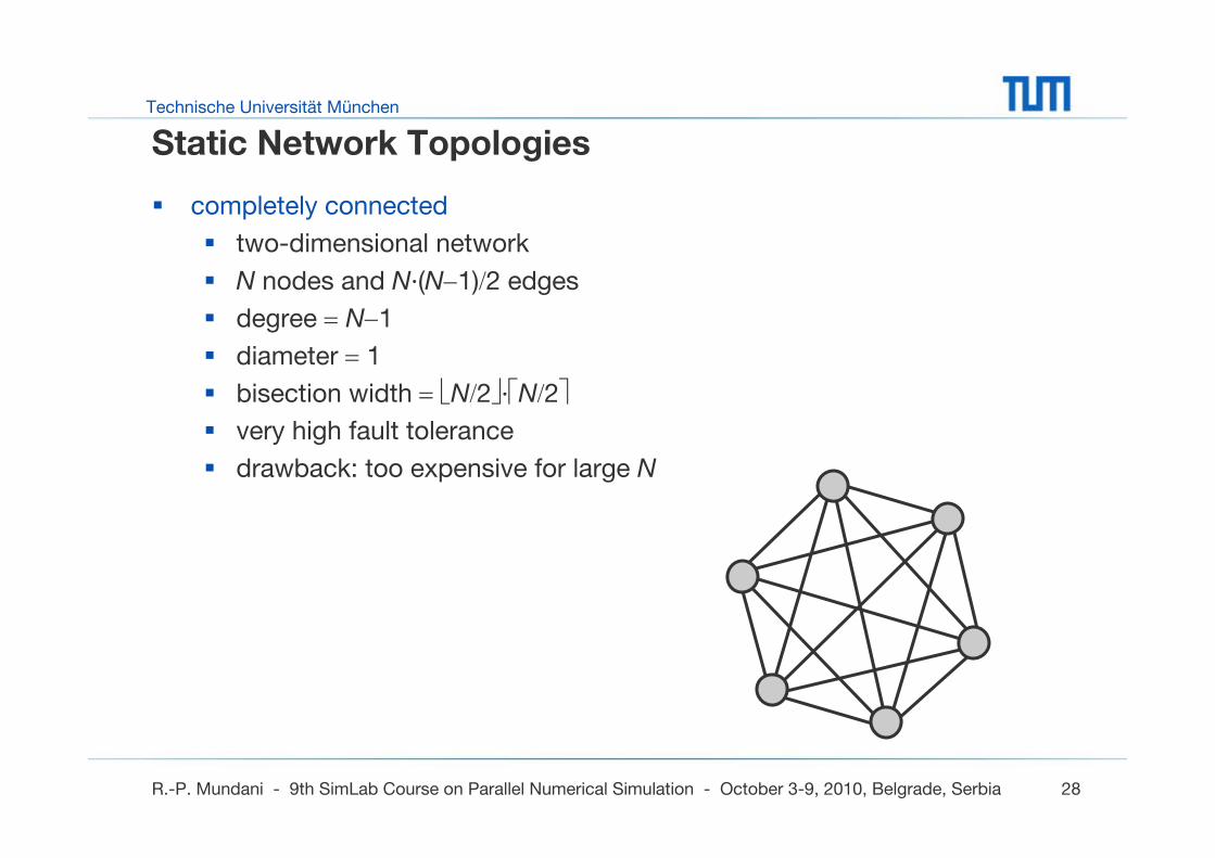
Static Network Topologies
completely connected
two-dimensional network
N nodes and N·(N−1)/2 edges
degree = N−1
diameter = 1
bisection width = ⎣N/2⎦·⎡N/2⎤very high fault tolerance
drawback: too expensive for large N
Technische Universität München
R.-P. Mundani - 9th SimLab Course on Parallel Numerical Simulation - October 3-9, 2010, Belgrade, Serbia 29
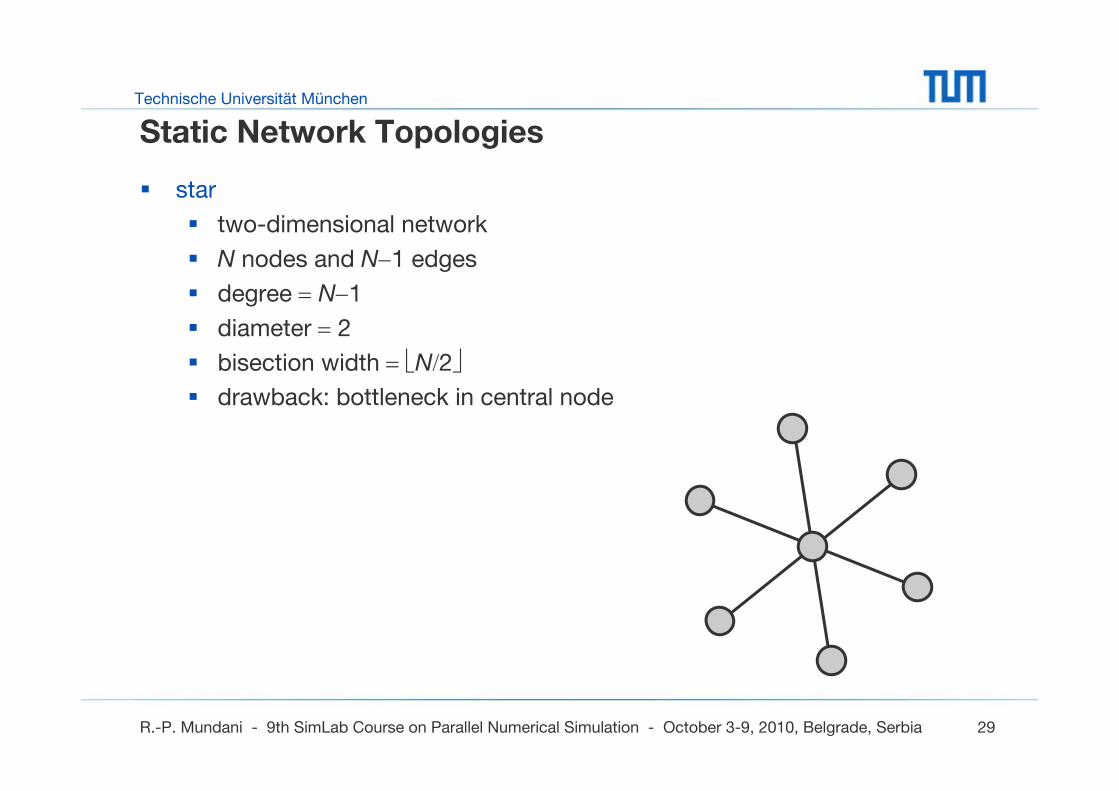
Static Network Topologies
star
two-dimensional network
N nodes and N−1 edges
degree = N−1
diameter = 2
bisection width = ⎣N/2⎦drawback: bottleneck in central node
Technische Universität München
R.-P. Mundani - 9th SimLab Course on Parallel Numerical Simulation - October 3-9, 2010, Belgrade, Serbia 30
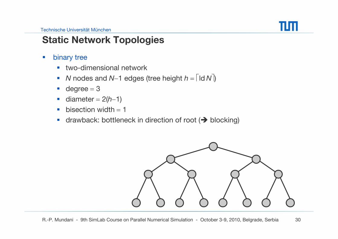
Static Network Topologies
binary tree
two-dimensional network
N nodes and N−1 edges (tree height h = ⎡ld N⎤)degree = 3
diameter = 2(h−1)
bisection width = 1
drawback: bottleneck in direction of root ( blocking)
Technische Universität München
R.-P. Mundani - 9th SimLab Course on Parallel Numerical Simulation - October 3-9, 2010, Belgrade, Serbia 31
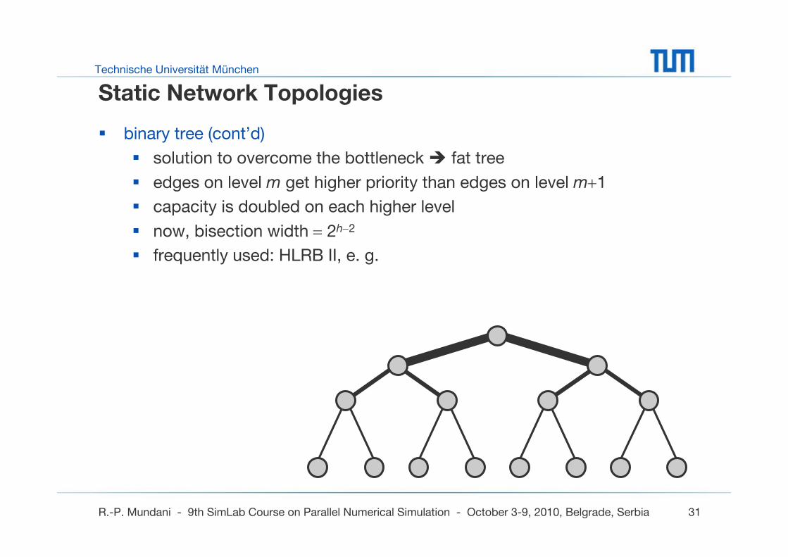
Static Network Topologies
binary tree (cont’d)
solution to overcome the bottleneck fat tree
edges on level m get higher priority than edges on level m+1
capacity is doubled on each higher level
now, bisection width = 2h−2
frequently used: HLRB II, e. g.
Technische Universität München
R.-P. Mundani - 9th SimLab Course on Parallel Numerical Simulation - October 3-9, 2010, Belgrade, Serbia 32
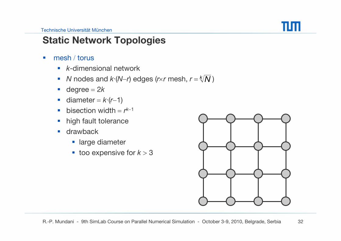
Static Network Topologies
mesh / torus
k-dimensional network
N nodes and k·(N−r) edges (r×r mesh, r = )
degree = 2k
diameter = k·(r−1)
bisection width = rk−1
high fault tolerance
drawback
large diameter
too expensive for k > 3
k N
Technische Universität München
R.-P. Mundani - 9th SimLab Course on Parallel Numerical Simulation - October 3-9, 2010, Belgrade, Serbia 33
Static Network Topologies
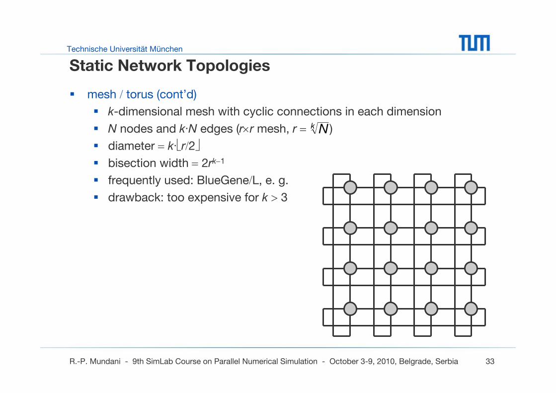
mesh / torus (cont’d)
k-dimensional mesh with cyclic connections in each dimension
N nodes and k·N edges (r×r mesh, r = )
diameter = k·⎣r/2⎦bisection width = 2rk−1
frequently used: BlueGene/L, e. g.
drawback: too expensive for k > 3
k N
Technische Universität München
R.-P. Mundani - 9th SimLab Course on Parallel Numerical Simulation - October 3-9, 2010, Belgrade, Serbia 34
Static Network Topologies
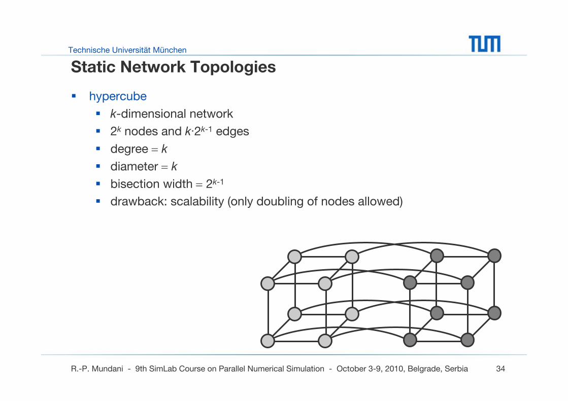
hypercube
k-dimensional network
2k nodes and k·2k-1 edges
degree = k
diameter = k
bisection width = 2k-1
drawback: scalability (only doubling of nodes allowed)
Technische Universität München
R.-P. Mundani - 9th SimLab Course on Parallel Numerical Simulation - October 3-9, 2010, Belgrade, Serbia 35
Static Network Topologies
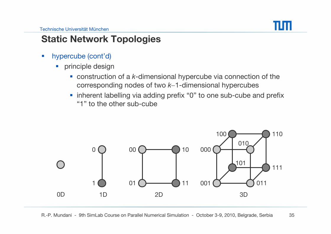
hypercube (cont’d)
principle design
construction of a k-dimensional hypercube via connection of the corresponding nodes of two k−1-dimensional hypercubes
inherent labelling via adding prefix “0” to one sub-cube and prefix “1” to the other sub-cube
0D
00
01
10
11
2D
001
000
011
010
100 110
101111
3D
0
1
1D
Technische Universität München
R.-P. Mundani - 9th SimLab Course on Parallel Numerical Simulation - October 3-9, 2010, Belgrade, Serbia 36
Dynamic Network Topologies
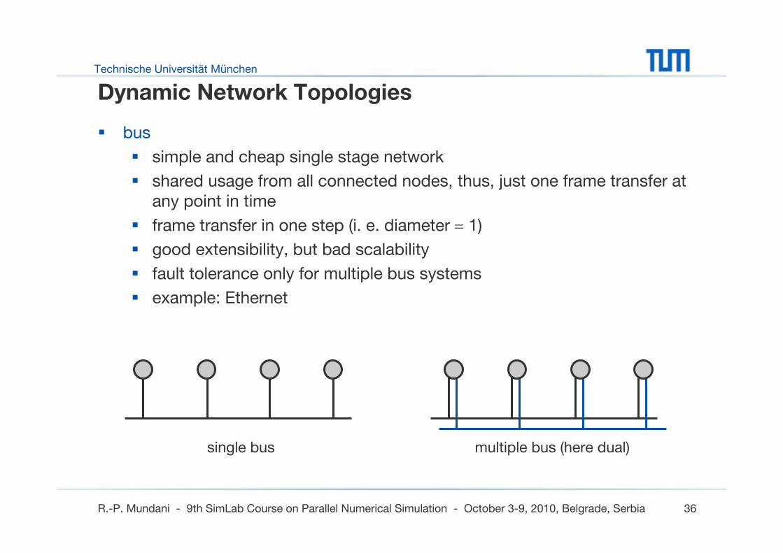
bus
simple and cheap single stage network
shared usage from all connected nodes, thus, just one frame transfer at any point in time
frame transfer in one step (i. e. diameter = 1)
good extensibility, but bad scalability
fault tolerance only for multiple bus systems
example: Ethernet
single bus multiple bus (here dual)
Technische Universität München
R.-P. Mundani - 9th SimLab Course on Parallel Numerical Simulation - October 3-9, 2010, Belgrade, Serbia 37
Dynamic Network Topologies
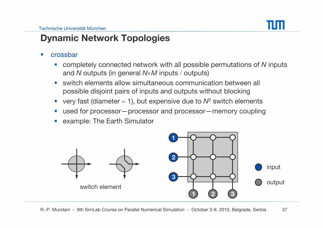
crossbar
completely connected network with all possible permutations of N inputs and N outputs (in general N×M inputs / outputs)
switch elements allow simultaneous communication between all possible disjoint pairs of inputs and outputs without blocking
very fast (diameter = 1), but expensive due to N2 switch elements
used for processor—processor and processor—memory coupling
example: The Earth Simulator
switch element
1
2
3
1 2 3
input
output
Technische Universität München
R.-P. Mundani - 9th SimLab Course on Parallel Numerical Simulation - October 3-9, 2010, Belgrade, Serbia 38
Overview
motivation
supercomputers
network topologies
terms and definitions
Technische Universität München
R.-P. Mundani - 9th SimLab Course on Parallel Numerical Simulation - October 3-9, 2010, Belgrade, Serbia 39
Terms and Definitions
quantitative performance evaluation
correlation of multi- and monoprocessor systems’ performance
important: program that can be executed on both systems
definitions
P(1): amount of unit operations of a program on the monoprocessorsystem
P(p): amount of unit operations of a program on the multiprocessor systems with p processors
T(1): execution time of a program on the monoprocessor system (measured in steps or clock cycles)
T(p): execution time of a program on the multiprocessor system (measured in steps or clock cycles) with p processors
Technische Universität München
R.-P. Mundani - 9th SimLab Course on Parallel Numerical Simulation - October 3-9, 2010, Belgrade, Serbia 40
Terms and Definitions
quantitative performance evaluation (cont’d)
simplifying preconditions
T(1) = P(1)
one operation to be executed in one step on the monoprocessor system
T(p) ≤ P(p)
more than one operation to be executed in one step (for p ≥ 2) on the multiprocessor system with p processors
Technische Universität München
R.-P. Mundani - 9th SimLab Course on Parallel Numerical Simulation - October 3-9, 2010, Belgrade, Serbia 41
Terms and Definitions
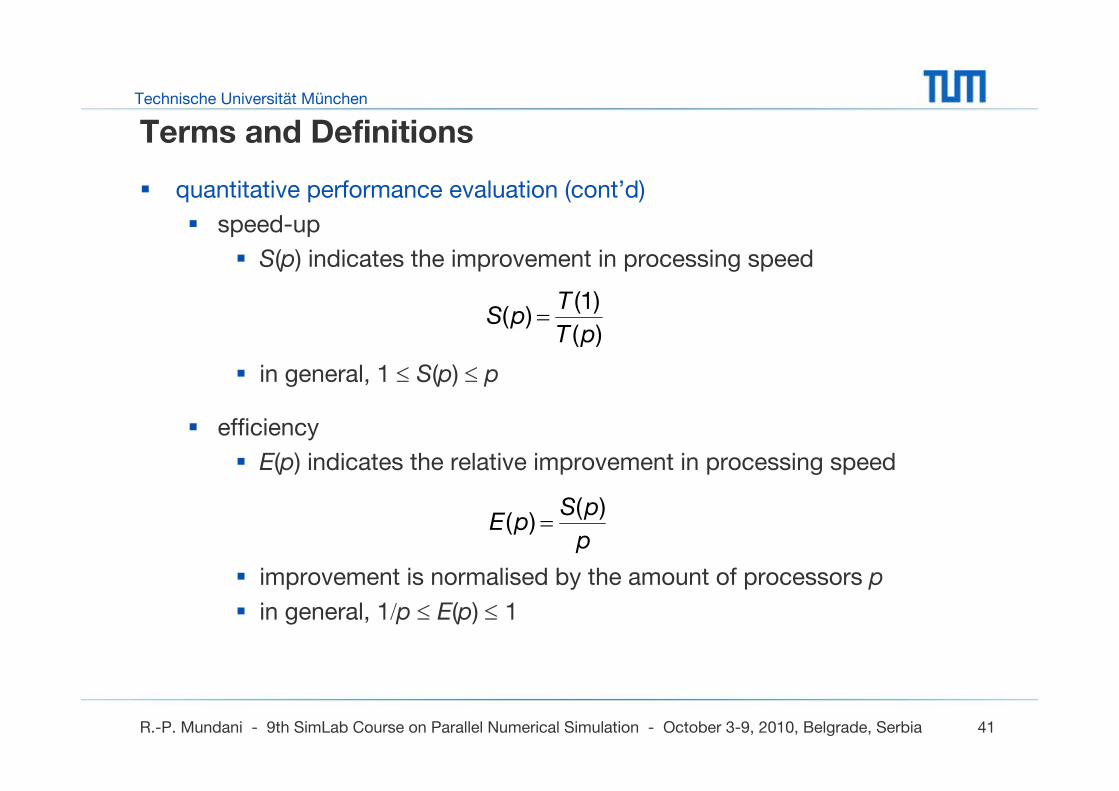
quantitative performance evaluation (cont’d)
speed-up
S(p) indicates the improvement in processing speed
in general, 1 ≤ S(p) ≤ p
efficiency
E(p) indicates the relative improvement in processing speed
improvement is normalised by the amount of processors p
in general, 1/p ≤ E(p) ≤ 1
)(
(1))(
pT
TpS =
p
pSpE
)()( =
Technische Universität München
R.-P. Mundani - 9th SimLab Course on Parallel Numerical Simulation - October 3-9, 2010, Belgrade, Serbia 42
Terms and Definitions
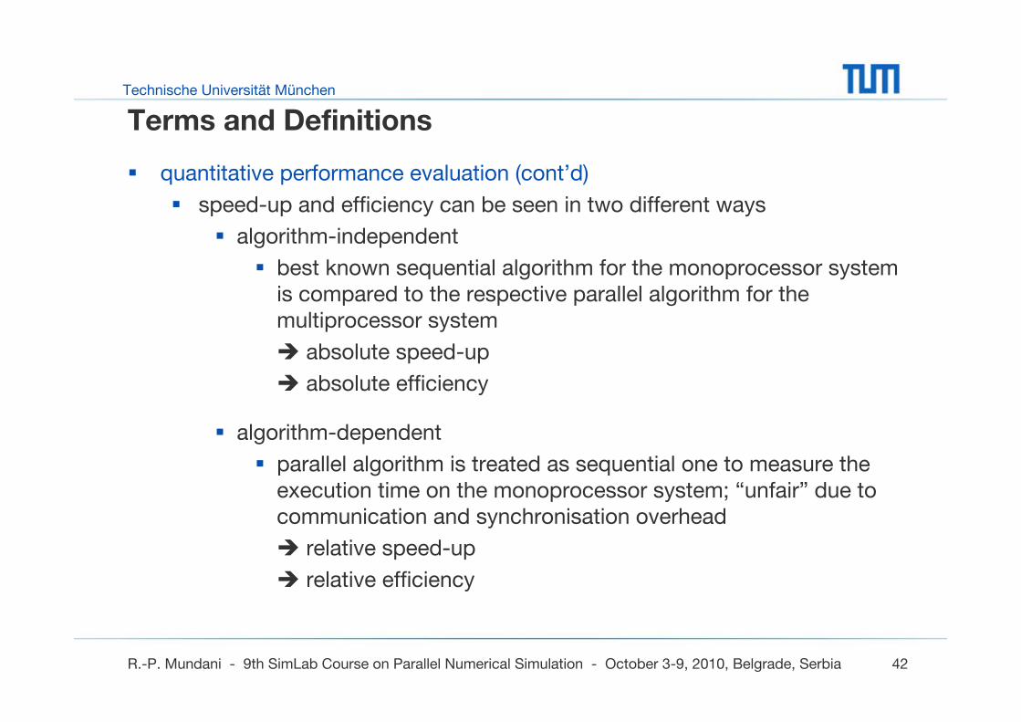
quantitative performance evaluation (cont’d)
speed-up and efficiency can be seen in two different ways
algorithm-independent
best known sequential algorithm for the monoprocessor system is compared to the respective parallel algorithm for the multiprocessor system
absolute speed-up
absolute efficiency
algorithm-dependent
parallel algorithm is treated as sequential one to measure the execution time on the monoprocessor system; “unfair” due to communication and synchronisation overhead
relative speed-up
relative efficiency
Technische Universität München
R.-P. Mundani - 9th SimLab Course on Parallel Numerical Simulation - October 3-9, 2010, Belgrade, Serbia 43
Terms and Definitions
general design questions
several considerations have to be taken into account for writing a parallel program (either from scratch or based on an existing sequential program)
standard questions comprise
which part of the (sequential) program can be parallelised
what kind of structure to be used for parallelisation
which parallel programming model to be used
what kind of compiler to be used
what about load balancing strategies
what kind of architecture is the target machine
and, better education necessary (“How many files…”)
Technische Universität München
R.-P. Mundani - 9th SimLab Course on Parallel Numerical Simulation - October 3-9, 2010, Belgrade, Serbia 44
Terms and Definitions
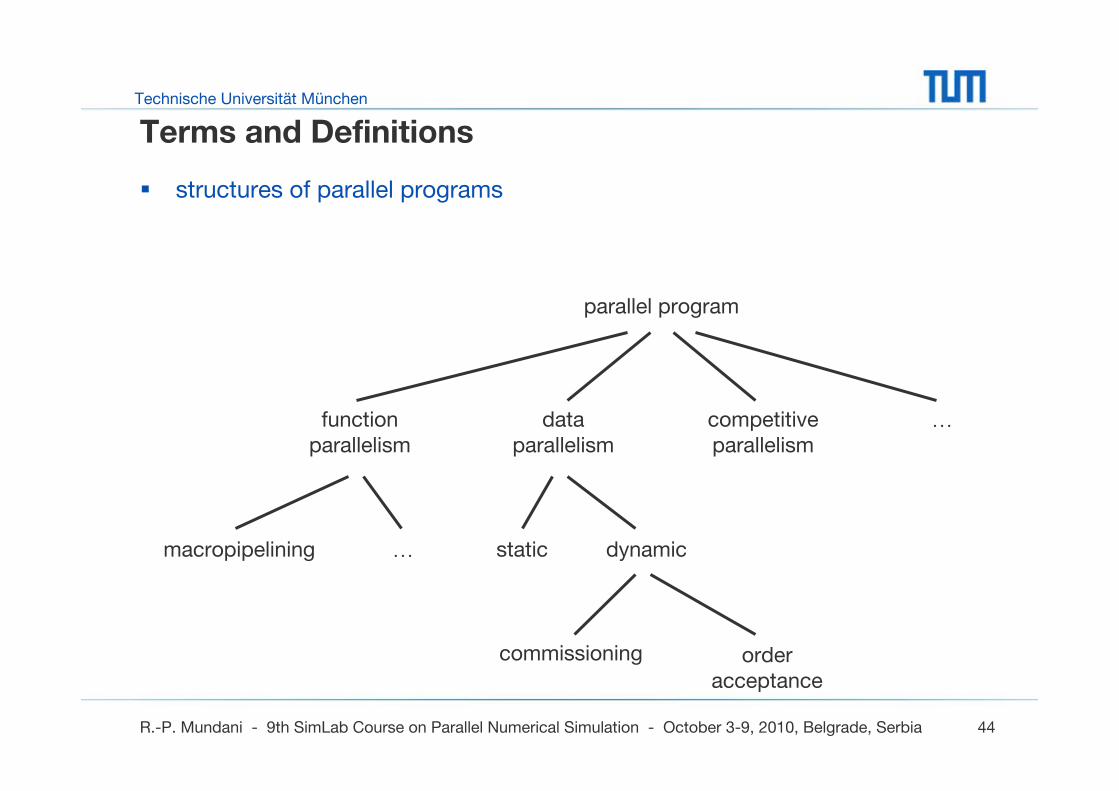
structures of parallel programs
parallel program
…macropipelining dynamicstatic
…competitiveparallelism
dataparallelism
functionparallelism
commissioning order acceptance
Technische Universität München
R.-P. Mundani - 9th SimLab Course on Parallel Numerical Simulation - October 3-9, 2010, Belgrade, Serbia 45
Terms and Definitions
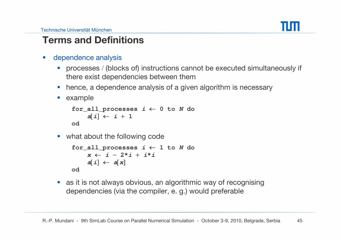
dependence analysis
processes / (blocks of) instructions cannot be executed simultaneously if there exist dependencies between them
hence, a dependence analysis of a given algorithm is necessary
example
for_all_processes i ← 0 to N doa[i] ← i + 1
od
what about the following code
for_all_processes i ← 1 to N dox ← i − 2*i + i*ia[i] ← a[x]
od
as it is not always obvious, an algorithmic way of recognising dependencies (via the compiler, e. g.) would preferable
Technische Universität München
R.-P. Mundani - 9th SimLab Course on Parallel Numerical Simulation - October 3-9, 2010, Belgrade, Serbia 46
Terms and Definitions
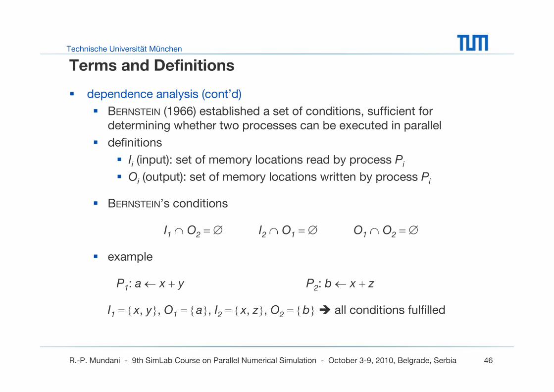
dependence analysis (cont’d)
BERNSTEIN (1966) established a set of conditions, sufficient for determining whether two processes can be executed in parallel
definitions
Ii (input): set of memory locations read by process Pi
Oi (output): set of memory locations written by process Pi
BERNSTEIN’s conditions
I1 ∩ O2 = ∅ I2 ∩ O1 = ∅ O1 ∩ O2 = ∅
example
P1: a ← x + y P2: b ← x + z
I1 = {x, y}, O1 = {a}, I2 = {x, z}, O2 = {b} all conditions fulfilled
Technische Universität München
R.-P. Mundani - 9th SimLab Course on Parallel Numerical Simulation - October 3-9, 2010, Belgrade, Serbia 47
Terms and Definitions
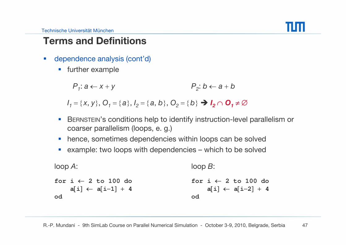
dependence analysis (cont’d)
further example
P1: a ← x + y P2: b ← a + b
I1 = {x, y}, O1 = {a}, I2 = {a, b}, O2 = {b} I2 ∩ O1 ≠ ∅
BERNSTEIN’s conditions help to identify instruction-level parallelism or coarser parallelism (loops, e. g.)
hence, sometimes dependencies within loops can be solved
example: two loops with dependencies – which to be solved
loop A: loop B:
for i ← 2 to 100 do for i ← 2 to 100 doa[i] ← a[i−1] + 4 a[i] ← a[i−2] + 4
od od
Technische Universität München
R.-P. Mundani - 9th SimLab Course on Parallel Numerical Simulation - October 3-9, 2010, Belgrade, Serbia 48
Terms and Definitions
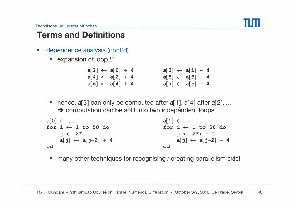
dependence analysis (cont’d)
expansion of loop B
a[2] ← a[0] + 4 a[3] ← a[1] + 4a[4] ← a[2] + 4 a[5] ← a[3] + 4a[6] ← a[4] + 4 a[7] ← a[5] + 4
hence, a[3] can only be computed after a[1], a[4] after a[2], …computation can be split into two independent loops
a[0] ← … a[1] ← …for i ← 1 to 50 do for i ← 1 to 50 do
j ← 2*i j ← 2*i + 1a[j] ← a[j−2] + 4 a[j] ← a[j−2] + 4
od od
many other techniques for recognising / creating parallelism exist
… …

Technische Universität München
R.-P. Mundani - 9th SimLab Course on Parallel Numerical Simulation - October 3-9, 2010, Belgrade, Serbia 49