basics of image deblurring - department of math/cs - …nagy/courses/fall06/id_lecture1.pdfbasics of...
TRANSCRIPT

Basics of Image Deblurring
Basics of Image Deblurring
Math 561
Fall, 2006

Basics of Image Deblurring
Outline
Introduction
Mathematical Model
The Computational Problem
Filtering Algorithms
Fast Computational Methods for FilteringBCCB MatricesSymmetric Toeplitz-plus-Hankel MatricesKronecker Product Matrices

Basics of Image Deblurring
Introduction
Image Restoration: Simple Example
I Given blurred image, and someinformation about the blurring.
I Goal: Compute approximation oftrue image.

Basics of Image Deblurring
Introduction
Image Restoration: Simple Example
I Given blurred image, and someinformation about the blurring.
I Goal: Compute approximation oftrue image.

Basics of Image Deblurring
Introduction
Applications: Astronomy
Viewing distant star fields using ground based telescopes.
Observed data Restored data

Basics of Image Deblurring
Introduction
Applications: Space Observations
Viewing space vehicles, satellites and other space junk.
Observed data Restored data

Basics of Image Deblurring
Introduction
Applications: Medical Imaging
Observed data Restored data
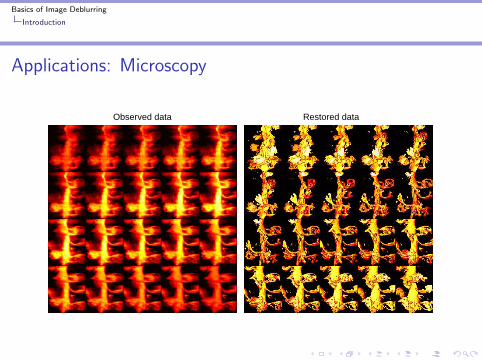
Basics of Image Deblurring
Introduction
Applications: Microscopy
Observed data Restored data

Basics of Image Deblurring
Introduction
Applications: Iris Recognition
Observed data Restored data

Basics of Image Deblurring
Mathematical Model
Mathematical Model of Image Formation
b(u, v) =
∫ ∫a(u, s, v , t)x(s, t)ds dt + e(u, v)
u
v
s
t

Basics of Image Deblurring
Mathematical Model
”Convolution” implies shift invariance
b(u, v) =
∫ ∫a(u − s, v − t)x(s, t)ds dt + e(u, v)
u
v
s
t
Basics of Image Deblurring
Mathematical Model
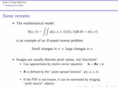
Some remarks
I The mathematical model:
b(u, v) =
∫ ∫a(u, s, v , t)x(s, t)ds dt + e(u, v)
is an example of an ill-posed inverse problem.
Small changes in e ⇒ large changes in x .
I Images are usually discrete pixel values, not functions!I Can approximate by matrix-vector equation: b = Ax + e
I A is defined by the ”point spread function” a(u, s, v , t).
I If the PSF is not known, it can be estimated by imaging”point source” objects.

Basics of Image Deblurring
Mathematical Model
Generating Experimental Point Spread Function
Point Source Object PSF: Picture of Point Source Object

Basics of Image Deblurring
The Computational Problem
The Computational Problem
From the matrix-vector equation
b = Ax + e
I Given b and A (or the PSF), compute an approximation of x
I Regarding the noise, e:I It is usually not known.I However, some statistical information may be known.I It is usually small, but it cannot be ignored!
That is, solving the linear algebra problem:
Ax = b ⇒ x = A−1b
usually does not work.

Basics of Image Deblurring
The Computational Problem
SVD Analysis
An important linear algebra tool: Singular Value Decomposition
Let A = UΣVT where
I Σ =diag(σ1, σ2, . . . , σn) , σ1 ≥ σ2 ≥ · · · ≥ σn ≥ 0
I UTU = I , VTV = I

Basics of Image Deblurring
The Computational Problem
SVD Analysis
An important linear algebra tool: Singular Value Decomposition
Let A = UΣVT where
I Σ =diag(σ1, σ2, . . . , σn) , σ1 ≥ σ2 ≥ · · · ≥ σn ≥ 0
I UTU = I , VTV = I
For image restoration problems,
I σ1 ≈ 1, small singular values cluster at 0
I small singular values ⇒ oscillating singular vectors

Basics of Image Deblurring
The Computational Problem
SVD Analysis
The naıve inverse solution can then be represented as:
x = A−1b
= VΣ−1UTb
=n∑
i=1
uTi b
σivi

Basics of Image Deblurring
The Computational Problem
SVD Analysis
The naıve inverse solution can then be represented as:
x = A−1(b + e)
= VΣ−1UT (b + e)
=n∑
i=1
uTi (b + e)
σivi
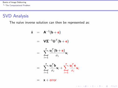
Basics of Image Deblurring
The Computational Problem
SVD Analysis
The naıve inverse solution can then be represented as:
x = A−1(b + e)
= VΣ−1UT (b + e)
=n∑
i=1
uTi (b + e)
σivi
=n∑
i=1
uTi b
σivi +
n∑i=1
uTi e
σivi
= x + error

Basics of Image Deblurring
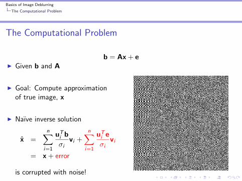
The Computational Problem
The Computational Problem
b = Ax + eI Given b and A
I Goal: Compute approximationof true image, x
I Naıve inverse solution
x =n∑
i=1
uTi b
σivi +
n∑i=1
uTi e
σivi
= x + error
is corrupted with noise!

Basics of Image Deblurring
The Computational Problem
The Computational Problem
b = Ax + eI Given b and A
I Goal: Compute approximationof true image, x
I Naıve inverse solution
x =n∑
i=1
uTi b
σivi +
n∑i=1
uTi e
σivi
= x + error
is corrupted with noise!
Basics of Image Deblurring
The Computational Problem
The Computational Problem
b = Ax + eI Given b and A
I Goal: Compute approximationof true image, x
I Naıve inverse solution
x =n∑
i=1
uTi b
σivi +
n∑i=1
uTi e
σivi
= x + error
is corrupted with noise!

Basics of Image Deblurring
Filtering Algorithms
Basic Idea of Filtering
Basic Idea: Filter out effects of small singular values.
xreg =n∑
i=1
φiuT
i b
σivi
where the ”filter factors” satisfy
φi ≈{
1 if σi is large0 if σi is small

Basics of Image Deblurring
Filtering Algorithms
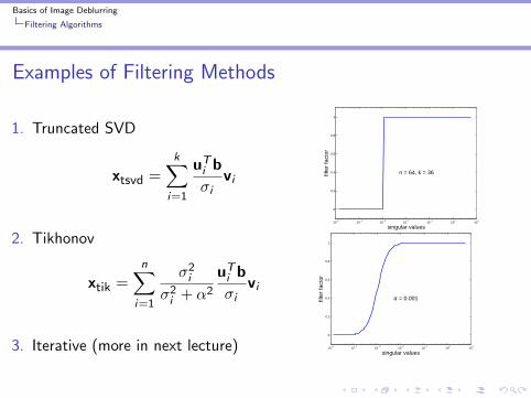
Examples of Filtering Methods
1. Truncated SVD
xtsvd =k∑
i=1
uTi b
σivi
2. Tikhonov
xtik =n∑
i=1
σ2i
σ2i + α2
uTi b
σivi
3. Iterative (more in next lecture)
Basics of Image Deblurring
Filtering Algorithms
Examples of Filtering Methods
1. Truncated SVD
xtsvd =k∑
i=1
uTi b
σivi
2. Tikhonov
xtik =n∑
i=1
σ2i
σ2i + α2
uTi b
σivi
3. Iterative (more in next lecture)
10−5
10−4
10−3
10−2
10−1
100
101
0
0.2
0.4
0.6
0.8
1
singular values
filte
r fa
ctor
n = 64, k = 36
10−5
10−4
10−3
10−2
10−1
100
101
0
0.2
0.4
0.6
0.8
1
singular values
filte
r fa
ctor
α = 0.001

Basics of Image Deblurring
Filtering Algorithms
Choosing Regularization Parameters
Lots of choices: Generalized Cross Validation (GCV), L-curve,discrepancy principle, ...

Basics of Image Deblurring
Filtering Algorithms
Choosing Regularization Parameters
Lots of choices: Generalized Cross Validation (GCV), L-curve,discrepancy principle, ...
GCV and Tikhonov: Choose λ to minimize
GCV(λ) =
nn∑
i=1
(uT
i b
σ2i + λ2
)2
(n∑
i=1
1
σ2i + λ2
)2

Basics of Image Deblurring
Filtering Algorithms
Choosing Regularization Parameters
Lots of choices: Generalized Cross Validation (GCV), L-curve,discrepancy principle, ...
GCV and Tikhonov: Choose λ to minimize
GCV(λ) =
nn∑
i=1
(uT
i b
σ2i + λ2
)2
(n∑
i=1
1
σ2i + λ2
)2
For L-curve, see G. Rodriguez.

Basics of Image Deblurring
Fast Computational Methods for Filtering
Remarks on Computational Methods
I SVD filtering can be computationally expensive.
I Further simplifying approximations are often used to obtainmore efficient algorithms:
I Spatial invariance and periodic boundary conditions:I A is circulant.I Can replace SVD with fast Fourier transforms (FFT).
I Other fast transforms (e.g., DCT) can sometimes be used.
I Separable blur ⇒ A can be decomposed using Kroneckerproducts:
A = Ar ⊗ Ac
Basics of Image Deblurring
Fast Computational Methods for Filtering
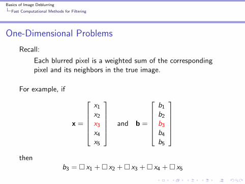
One-Dimensional Problems
Recall:
Each blurred pixel is a weighted sum of the correspondingpixel and its neighbors in the true image.
For example, if
x =
x1
x2
x3
x4
x5
and b =
b1
b2
b3
b4
b5
then
b3 = � x1 + � x2 + � x3 + � x4 + � x5

Basics of Image Deblurring
Fast Computational Methods for Filtering
One-Dimensional Problems
The weights come from the PSF:
For example, if
x =
x1
x2
x3
x4
x5
, p =
p1
p2
p3
p4
p5
and b =
b1
b2
b3
b4
b5
then

Basics of Image Deblurring
Fast Computational Methods for Filtering
One-Dimensional Problems
The weights come from the PSF:
For example, if
x =
x1
x2
x3
x4
x5
,
p5
p4
p3
p2
p1
and b =
b1
b2
b3
b4
b5
then
1. Rotate the PSF, p, by 180 degrees about center.

Basics of Image Deblurring
Fast Computational Methods for Filtering
One-Dimensional Problems
The weights come from the PSF:
For example, ifx1
x2
x3
x4
x5
p5
p4
p3
p2
p1
and b =
b1
b2
b3
b4
b5
then
2. Match coefficients of rotated PSF and x

Basics of Image Deblurring
Fast Computational Methods for Filtering
One-Dimensional Problems
The weights come from the PSF:
For example, ifx1
x2
x3
x4
x5
p5
p4
p3
p2
p1
and b =
b1
b2
b3
b4
b5
then
3. Multiply corresponding components and sum.
Basics of Image Deblurring
Fast Computational Methods for Filtering
One-Dimensional Problems
The weights come from the PSF:
For example, ifx1
x2
x3
x4
x5
p5
p4
p3
p2
p1
and b =
b1
b2
b3
b4
b5
then
b3 = p5x1 + p4x2 + p3x3 + p2x4 + p1x5

Basics of Image Deblurring
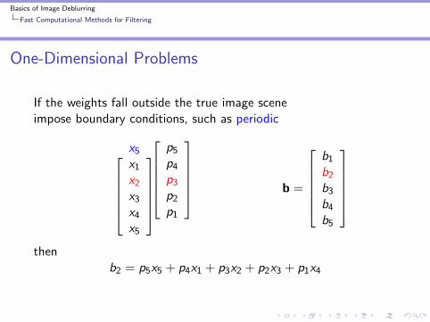
Fast Computational Methods for Filtering
One-Dimensional Problems
If the weights fall outside the true image scene
?x1
x2
x3
x4
x5
p5
p4
p3
p2
p1
b =
b1
b2
b3
b4
b5
then
b2 = p5 ? + p4x1 + p3x2 + p2x3 + p1x4

Basics of Image Deblurring
Fast Computational Methods for Filtering
One-Dimensional Problems
If the weights fall outside the true image sceneimpose boundary conditions
wx1
x2
x3
x4
x5
p5
p4
p3
p2
p1
b =
b1
b2
b3
b4
b5
then
b2 = p5 w + p4x1 + p3x2 + p2x3 + p1x4

Basics of Image Deblurring
Fast Computational Methods for Filtering
One-Dimensional Problems
If the weights fall outside the true image sceneimpose boundary conditions, such as zero
0x1
x2
x3
x4
x5
p5
p4
p3
p2
p1
b =
b1
b2
b3
b4
b5
then
b2 = p4x1 + p3x2 + p2x3 + p1x4
Basics of Image Deblurring
Fast Computational Methods for Filtering
One-Dimensional Problems
If the weights fall outside the true image sceneimpose boundary conditions, such as periodic
x5x1
x2
x3
x4
x5
p5
p4
p3
p2
p1
b =
b1
b2
b3
b4
b5
then
b2 = p5x5 + p4x1 + p3x2 + p2x3 + p1x4

Basics of Image Deblurring
Fast Computational Methods for Filtering
One-Dimensional Problems
If the weights fall outside the true image sceneimpose boundary conditions, such as reflexive
x1x1
x2
x3
x4
x5
p5
p4
p3
p2
p1
b =
b1
b2
b3
b4
b5
then
b2 = p5x1 + p4x1 + p3x2 + p2x3 + p1x4

Basics of Image Deblurring
Fast Computational Methods for Filtering
One-Dimensional Problems
In general, we can write
b1
b2
b3
b4
b5
=
p5 p4 p3 p2 p1
p5 p4 p3 p2 p1
p5 p4 p3 p2 p1
p5 p4 p3 p2 p1
p5 p4 p3 p2 p1
w1
w2
x1
x2
x3
x4
x5
y1
y2
where
I zero BC ⇒ wi = yi = 0
I periodic BC ⇒ w1 = x4, w2 = x5, y1 = x1, y2 = x2
I reflexive BC ⇒ w1 = x2, w2 = x1, y1 = x5, y2 = x4
Basics of Image Deblurring
Fast Computational Methods for Filtering
One-Dimensional Problems
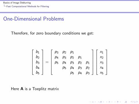
Therefore, for zero boundary conditions we get:
b1
b2
b3
b4
b5
=
p3 p2 p1
p4 p3 p2 p1
p5 p4 p3 p2 p1
p5 p4 p3 p2
p5 p4 p3
x1
x2
x3
x4
x5
Here A is a Toeplitz matrix

Basics of Image Deblurring
Fast Computational Methods for Filtering
One-Dimensional Problems
For periodic boundary conditions we get:
b1
b2
b3
b4
b5
=
p3 p2 p1 p5 p4
p4 p3 p2 p1 p5
p5 p4 p3 p2 p1
p1 p5 p4 p3 p2
p2 p1 p5 p4 p3
x1
x2
x3
x4
x5
Here A is a circulant matrix

Basics of Image Deblurring
Fast Computational Methods for Filtering
One-Dimensional Problems
For reflexive boundary conditions we get:
b1
b2
b3
b4
b5
=
p3 p2 p1
p4 p3 p2 p1
p5 p4 p3 p2 p1
p5 p4 p3 p2
p5 p4 p3
+
p4 p5
p5
p1
p1 p2
x1
x2
x3
x4
x5
Here A is a Toeplitz-plus-Hankel

Basics of Image Deblurring
Fast Computational Methods for Filtering
Two-Dimensional Problems
With zero boundary conditions we obtain BTTB matrix:
b11
b21
b31
b12
b22
b32
b13
b23
b33
=
p22 p12 p21 p11
p32 p22 p12 p31 p21 p11
p32 p22 p31 p21
p23 p13 p22 p12 p21 p11
p33 p23 p13 p32 p22 p12 p31 p21 p11
p33 p23 p32 p22 p31 p21
p23 p13 p22 p12
p33 p23 p13 p32 p22 p12
p33 p23 p32 p22
x11
x21
x31
x12
x22
x32
x13
x23
x33
b = vec(B), p = vec(P), x = vec(X)

Basics of Image Deblurring
Fast Computational Methods for Filtering
Two-Dimensional Problems
Matrix structures:
I Zero boundary conditions ⇒ A is BTTB
I Periodic boundary conditions ⇒ A is BCCB
I Reflexive boundary conditions ⇒ A is sum of BTTB, BTHB,BHTB, BHHB
Legend:
BTTB: Block Toeplitz with Toeplitz blocks
BCCB: Block circulant with circulant blocks
BHHB: Block Hankel with Hankel blocks
BTHB: Block Toeplitz with Hankel blocks
BHTB: Block Hankel with Toeplitz blocks
Basics of Image Deblurring
Fast Computational Methods for Filtering
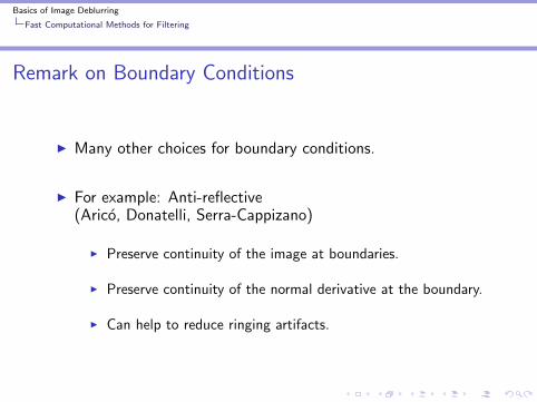
Remark on Boundary Conditions
I Many other choices for boundary conditions.
I For example: Anti-reflective(Arico, Donatelli, Serra-Cappizano)
I Preserve continuity of the image at boundaries.
I Preserve continuity of the normal derivative at the boundary.
I Can help to reduce ringing artifacts.

Basics of Image Deblurring
Fast Computational Methods for Filtering
Separable Two-Dimensional Blurs
Separable Blur ⇒ Horizontal and vertical components separate.
In this case, the PSF array has rank = 1:
P = rcT =
c1
c2
c3
[ r1 r2 r3]
=
c1r1 c1r2 c1r3c2r1 c2r2 c2r3c3r1 c3r2 c3r3

Basics of Image Deblurring
Fast Computational Methods for Filtering
Separable Two-Dimensional Blurs
Separable Blur ⇒ Horizontal and vertical components separate.
Forming the matrix with this special PSF we obtain (zero BC):
A =
c2r2 c1r2 c2r1 c1r1c3r2 c2r2 c1r2 c3r1 c2r1 c1r1
c3r2 c2r2 c3r1 c2r1c2r3 c1r3 c2r2 c1r2 c2r1 c1r1c3r3 c2r3 c1r3 c3r2 c2r2 c1r2 c3r1 c2r1 c1r1
c3r3 c2r3 c3r2 c2r2 c3r1 c2r1c2r3 c1r3 c2r2 c1r2c3r3 c2r3 c1r3 c3r2 c2r2 c1r2
c3r3 c2r3 c3r2 c2r2

Basics of Image Deblurring
Fast Computational Methods for Filtering
Separable Two-Dimensional Blurs
Separable Blur ⇒ Horizontal and vertical components separate.
Forming the matrix with this special PSF we obtain (zero BC):
A =
r2
c2 c1
c3 c2 c1
c3 c2
r1
c2 c1
c3 c2 c1
c3 c2
0
r3
c2 c1
c3 c2 c1
c3 c2
r2
c2 c1
c3 c2 c1
c3 c2
r1
c2 c1
c3 c2 c1
c3 c2
0 r3
c2 c1
c3 c2 c1
c3 c2
r2
c2 c1
c3 c2 c1
c3 c2

Basics of Image Deblurring
Fast Computational Methods for Filtering
Separable Two-Dimensional Blurs
Separable Blur ⇒ Horizontal and vertical components separate.
Forming the matrix with this special PSF we obtain (zero BC):
A = Ar ⊗ Ac
r2 r1r3 r2 r1
r3 r2
⊗ c2 c1
c3 c2 c1
c3 c2
Where ⊗ denotes Kronecker product.

Basics of Image Deblurring
Fast Computational Methods for Filtering
Separable Two-Dimensional Blurs
Similar structures occur for other boundary conditions:
A = Ar ⊗ Ac
whereI Zero boundary conditions:
I Ar is Toeplitz, defined by rI Ac is Topelitz, defined by c
I Periodic boundary conditions:I Ar is circulant, defined by rI Ac is circulant, defined by c
I Reflexive boundary conditions:I Ar is Toeplitz-plus-Hankel, defined by rI Ac is Toeplitz-plus-Hankel, defined by c

Basics of Image Deblurring
Fast Computational Methods for Filtering
Summary of Matrix Structures
BC Non-separable PSF Separable PSF
zero BTTB Kronecker of Toeplitz matrices
periodic BCCB Kronecker of circulant matrices
reflexive BTTB+BTHB Kronecker of+BHTB+BHHB Toeplitz-plus-Hankel matrices

Basics of Image Deblurring
Fast Computational Methods for Filtering
BCCB Matrices
BCCB Matrices
With periodic boundary conditions A is a BCCB matrix:
b11
b21
b31
b12
b22
b32
b13
b23
b33
=
p22 p12 p32 p21 p11 p31 p23 p13 p33
p32 p22 p12 p31 p21 p11 p33 p23 p13
p12 p32 p22 p11 p31 p21 p13 p33 p23
p23 p13 p33 p22 p12 p32 p21 p11 p31
p33 p23 p13 p32 p22 p12 p31 p21 p11
p13 p33 p23 p12 p32 p22 p11 p31 p21
p21 p11 p31 p23 p13 p33 p22 p12 p32
p31 p21 p11 p33 p23 p13 p32 p22 p12
p11 p31 p21 p13 p33 p23 p12 p32 p22
x11
x21
x31
x12
x22
x32
x13
x23
x33
b = vec(B), p = vec(P), x = vec(X)

Basics of Image Deblurring
Fast Computational Methods for Filtering
BCCB Matrices
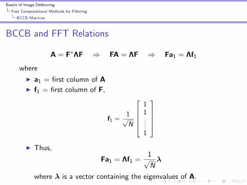
Important BCCB Matrix Property
I Every BCCB matrix has the same set of eigenvectors:
A = F∗ΛF
whereI F is the two-dimensional discrete Fourier transform matrixI F∗F = FF∗ = II Λ = diagonal containing eigenvalues of A
I Computations with F can be done very efficiently:
O(N log N)
using Fast Fourier Transforms (FFT)s.
Basics of Image Deblurring
Fast Computational Methods for Filtering
BCCB Matrices
BCCB and FFT Relations
A = F∗ΛF ⇒ FA = ΛF ⇒ Fa1 = Λf1
where
I a1 = first column of AI f1 = first column of F,
f1 =1√N
11...1
I Thus,
Fa1 = Λf1 =1√N
λ
where λ is a vector containing the eigenvalues of A.

Basics of Image Deblurring
Fast Computational Methods for Filtering
BCCB Matrices
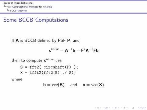
Some BCCB Computations
If A is BCCB defined by PSF P, and
b = Ax = F∗ΛFx
then to compute b use
S = fft2( circshift(P) );B = ifft2(S .* fft2(X));
whereb = vec(B) and x = vec(X)
Basics of Image Deblurring
Fast Computational Methods for Filtering
BCCB Matrices
Some BCCB Computations
If A is BCCB defined by PSF P, and
xnaive = A−1b = F∗Λ−1Fb
then to compute xnaive use
S = fft2( circshift(P) );X = ifft2(fft2(B) ./ S);
whereb = vec(B) and x = vec(X)
Basics of Image Deblurring
Fast Computational Methods for Filtering
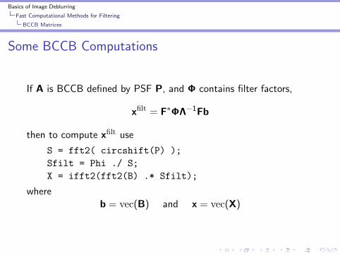
BCCB Matrices
Some BCCB Computations
If A is BCCB defined by PSF P, and Φ contains filter factors,
xfilt = F∗ΦΛ−1Fb
then to compute xfilt use
S = fft2( circshift(P) );Sfilt = Phi ./ S;X = ifft2(fft2(B) .* Sfilt);
whereb = vec(B) and x = vec(X)

Basics of Image Deblurring
Fast Computational Methods for Filtering
Symmetric Toeplitz-plus-Hankel Matrices
Summary of Matrix Structures
BC Non-separable PSF Separable PSF
zero BTTB Kronecker of Toeplitz matrices
periodic BCCB Kronecker of circulant matrices
reflexive BTTB+BTHB Kronecker of+BHTB+BHHB Toeplitz-plus-Hankel matrices

Basics of Image Deblurring
Fast Computational Methods for Filtering
Symmetric Toeplitz-plus-Hankel Matrices
Toeplitz-plus-Hankel Matrices
With reflexive boundary conditions A is a
BTTB + BTHB + BHTB + BHHB
matrix defined by the PSF.
”Strong” symmetry condition: If
P =
0 0 0
0 P 00 0 0
where
I P is (2k − 1)× (2k − 1) with center located at the (k, k)
I P = fliplr(P) = flipud(P) = fliplr(flipud(P))

Basics of Image Deblurring
Fast Computational Methods for Filtering
Symmetric Toeplitz-plus-Hankel Matrices
BTTB+BTHB+BHTB+BHHB Matrix Properties
If the PSF satisfies strong symmetry condition, then:
I A is symmetric
I A is block symmetric
I Each block in A is symmetric
I A has the spectral decomposition
A = CTΛC
where C is the two-dimensional discrete cosine transform(DCT) matrix.
I As with FFTs, computations with C cost O(N log N).

Basics of Image Deblurring
Fast Computational Methods for Filtering
Symmetric Toeplitz-plus-Hankel Matrices
Toeplitz-plus-Hankel and DCT Relations
A = CTΛC ⇒ CA = ΛC ⇒ Ca1 = Λc1
where
I a1 = first column of A
I c1 = first column of C,
I Thus, the eigenvalues of C are given by
Ca1 = Λc1 ⇒ λi =[Ca1]i[c1]i

Basics of Image Deblurring
Fast Computational Methods for Filtering
Symmetric Toeplitz-plus-Hankel Matrices
Additional DCT Computations
If A is defined by strongly symmetric PSF with reflexive boundaryconditions, and
b = Ax = CTΛCx
then to compute b use
e1 = zeros(size(P));, e1(1,1) = 1;S = dct2( dctshift(P) ) ./ dct2(e1);B = idct2(S .* dct2(X));
whereb = vec(B) and x = vec(X)

Basics of Image Deblurring
Fast Computational Methods for Filtering
Symmetric Toeplitz-plus-Hankel Matrices
Additional DCT Computations
If A is defined by strongly symmetric PSF with reflexive boundaryconditions, and
xnaive = A−1b = CTΛ−1Cb
then to compute xnaive use
e1 = zeros(size(P));, e1(1,1) = 1;S = dct2( dctshift(P) ) ./ dct2(e1);X = idct2(dct2(B) ./ S);
whereb = vec(B) and x = vec(X)

Basics of Image Deblurring
Fast Computational Methods for Filtering
Symmetric Toeplitz-plus-Hankel Matrices
Additional DCT Computations
If A is defined by strongly symmetric PSF with reflexive boundaryconditions, and Φ contains filter factors,
xfilt = CTΦΛ−1Cb
then to compute xfilt use
e1 = zeros(size(P));, e1(1,1) = 1;S = dct2( dctshift(P) ) ./ dct2(e1);Sfilt = Phi ./ S;X = idct2(dct2(B) .* Sfilt);
whereb = vec(B) and x = vec(X)

Basics of Image Deblurring
Fast Computational Methods for Filtering
Kronecker Product Matrices
Summary of Matrix Structures
BC Non-separable PSF Separable PSF
zero BTTB Kronecker of Toeplitz matricesperiodic BCCB Kronecker of circulant matricesreflexive BTTB+BTHB Kronecker of
+BHTB+BHHB Toeplitz-plus-Hankel matricesreflexive BTTB+BTHB Kronecker of symmetric
strongly symmetric +BHTB+BHHB Toeplitz-plus-Hankel matrices
Basics of Image Deblurring
Fast Computational Methods for Filtering
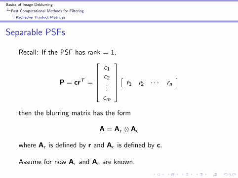
Kronecker Product Matrices
Separable PSFs
Recall: If the PSF has rank = 1,
P = crT =
c1
c2...
cm
[ r1 r2 · · · rn]
then the blurring matrix has the form
A = Ar ⊗ Ac
where Ar is defined by r and Ac is defined by c.
Assume for now Ar and Ac are known.

Basics of Image Deblurring
Fast Computational Methods for Filtering
Kronecker Product Matrices
Useful Kronecker Product Properties
I b = (Ar ⊗ Ac)x ⇔ B = AcXATr
where b = vec(B) and x = vec(X)
I (Ar ⊗ Ac)T = AT
r ⊗ ATc
I (Ar ⊗ Ac)−1 = A−1
r ⊗ A−1c
I (A(1)r ⊗ A(1)
c )(A(2)r ⊗ A(2)
c ) = (A(1)r A(2)
r )⊗ (A(1)c A(2)
c )

Basics of Image Deblurring
Fast Computational Methods for Filtering
Kronecker Product Matrices
Exploiting Kronecker Product Properties in Matlab
Using the property:
b = (Ar ⊗ Ac)x ⇔ B = AcXATr
in Matlab we can compute
B = Ac*X*Ar’;

Basics of Image Deblurring
Fast Computational Methods for Filtering
Kronecker Product Matrices
Exploiting Kronecker Product Properties in Matlab
Using the property:
b = (Ar ⊗ Ac)x ⇔ B = AcXATr
and if Ar and Ac are nonsingular,
(Ar ⊗ Ac)−1 = A−1
r ⊗ A−1c
we obtainX = A−1
c BA−Tr
In Matlab we can compute
X = Ac \ B / Ar’;

Basics of Image Deblurring
Fast Computational Methods for Filtering
Kronecker Product Matrices
Exploiting Kronecker Product Properties in Matlab
We can compute SVD of small matrices:
Ar = UrΣrVTr and Ac = UcΣcV
Tc
Then
A = Ar ⊗ Ac
= (UrΣrVTr )⊗ (UcΣcV
Tc )
= (Ur ⊗Uc)(Σr ⊗Σc)(Vr ⊗ Vc)T
= SVD of big matrix A
Note: Do not need to explicitly form big matrices
Ur ⊗Uc, Σr ⊗Σc, Vr ⊗ Vc

Basics of Image Deblurring
Fast Computational Methods for Filtering
Kronecker Product Matrices
Exploiting Kronecker Product Properties in Matlab
To compute inverse solution from SVD of small matrices:
xnaive = A−1b = VΣ−1UTb
is equivalent to
Xnaive = A−1c BA−T
r = VcΣ−1c UT
c BUrΣ−1r VT
r
A Matlab implementation could be:
[Ur, Sr, Vr] = svd(Ar);
[Uc, Sc, Vc] = svd(Ac);
S = diag(Sc) * diag(Sr)’;
X = Vc * ( (Uc’ * B * Ur)./S ) * Vr’;
Basics of Image Deblurring
Fast Computational Methods for Filtering
Kronecker Product Matrices
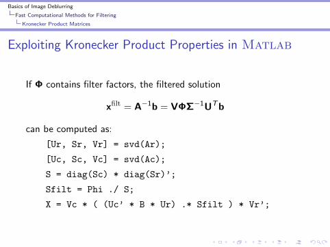
Exploiting Kronecker Product Properties in Matlab
If Φ contains filter factors, the filtered solution
xfilt = A−1b = VΦΣ−1UTb
can be computed as:
[Ur, Sr, Vr] = svd(Ar);
[Uc, Sc, Vc] = svd(Ac);
S = diag(Sc) * diag(Sr)’;
Sfilt = Phi ./ S;
X = Vc * ( (Uc’ * B * Ur) .* Sfilt ) * Vr’;

Basics of Image Deblurring
Fast Computational Methods for Filtering
Kronecker Product Matrices
Summary of Fast Algorithms
For spatially invariant PSFs, we have the following fast algorithms.
Boundary Matrix FastPSF condition structure algorithm
arbitrary periodic BCCB 2-d FFT
strongly symmetric reflexive sum of BXXB 2-d DCT
rank one arbitrary Kronecker product 2 SVDs

Basics of Image Deblurring
Fast Computational Methods for Filtering
Kronecker Product Matrices
Matlab Examples
Recall some examples of filtering methods:
1. Truncated SVD
xtsvd =k∑
i=1
uTi b
σivi
2. Tikhonov
xtik =n∑
i=1
σ2i
σ2i + α2
uTi b
σivi
3. Iterative (more in next lecture)
10−5
10−4
10−3
10−2
10−1
100
101
0
0.2
0.4
0.6
0.8
1
singular values
filte
r fa
ctor
n = 64, k = 36
10−5
10−4
10−3
10−2
10−1
100
101
0
0.2
0.4
0.6
0.8
1
singular values
filte
r fa
ctor
α = 0.001
Basics of Image Deblurring
Fast Computational Methods for Filtering
Kronecker Product Matrices
The End
I Image deblurring examples arise in many applications.
I Fast algorithms can produce good reconstructions for manyproblems.
I Further details and software can be found in:Deblurring Images: Matrices, Spectra and FilteringP. C. Hansen, J. G. Nagy and D. P. O’LearySIAM, 2006
http://www2.imm.dtu.dk/∼pch/HNO/
I Next time: Iterative methods for harder problems.