basic tail and concentration bounds - university of …mjwain/stat210b/chap2...example 2.1 (gaussian...
TRANSCRIPT

C H A P T E R 2 1
Basic tail and concentration bounds 2
In a variety of settings, it is of interest to obtain bounds on the tails of a random 3
variable, or two-sided inequalities that guarantee that a random variable is close to its 4
mean or median. In this chapter, we explore a number of elementary techniques for 5
obtaining both deviation and concentration inequalities. It is an entrypoint to more 6
advanced literature on large deviation bounds and concentration of measure. 7
2.1 Classical bounds 8
One way in which to control a tail probability P[X ≥ t] is by controlling the moments of 9
the random variable X. Gaining control of higher-order moments leads to correspond- 10
ingly sharper bounds on tail probabilities, ranging from Markov’s inequality (which 11
requires only existence of the first moment) to the Chernoff bound (which requires 12
existence of the moment generating function). 13
2.1.1 From Markov to Chernoff 14
The most elementary tail bound is Markov’s inequality : given a non-negative random
variable X with finite mean, we have
P[X ≥ t] ≤ E[X]
tfor all t > 0. (2.1)
For a random variable X that also has a finite variance, we have Chebyshev’s inequality :
P[|X − µ| ≥ t
]≤ var(X)
t2for all t > 0. (2.2)
Note that this is a simple form of concentration inequality, guaranteeing that X is 15
close to its mean µ whenever its variance is small. Chebyshev’s inequality follows by 16
applying Markov’s inequality to the non-negative random variable Y = (X − E[X])2. 17
Both Markov’s and Chebyshev’s inequality are sharp, meaning that they cannot be 18
improved in general (see Exercise 2.1). 19
There are various extensions of Markov’s inequality applicable to random variables
January 22, 2015 0age

12 CHAPTER 2. BASIC TAIL AND CONCENTRATION BOUNDS
with higher-order moments. For instance, whenever X has a central moment of order
k, an application of Markov’s inequality to the random variable |X − µ|k yields that
P[|X − µ| ≥ t] ≤ E[|X − µ|k]tk
for all t > 0. (2.3)
Of course, the same procedure can be applied to functions other than polynomials
|X − µ|k. For instance, suppose that the random variable X has a moment generating
function in a neighborhood of zero, meaning that that there is some constant b > 0
such that the function ϕ(λ) = E[eλ(X−µ)] exists for all λ ≤ |b|. In this case, for any
λ ∈ [0, b], we may apply Markov’s inequality to the random variable Y = eλ(X−µ),thereby obtaining the upper bound
P[(X − µ) ≥ t] = P[eλ(X−µ) ≥ eλt] ≤ E[eλ(X−µ)]eλt
. (2.4)
Optimizing our choice of λ so as to obtain the tightest result yields the Chernoff bound—
namely, the inequality
logP[(X − µ) ≥ t] ≤ − supλ∈[0,b]
λt− logE[eλ(X−µ)]
. (2.5)
As we explore in Exercise 2.3, the moment bound (2.3) with the optimal choice of k is1
never worse than the bound (2.5) based on the moment-generating function. Nonethe-2
less, the Chernoff bound is most widely used in practice, possibly due to the ease of3
manipulating moment generating functions. Indeed, a variety of important tail bounds4
can be obtained as particular cases of inequality (2.5), as we discuss in examples to5
follow.6
2.1.2 Sub-Gaussian variables and Hoeffding bounds7
The form of tail bound obtained via the the Chernoff approach depends on the growth8
rate of the moment generating function. Accordingly, in the study of tail bounds, it9
is natural to classify random variables in terms of their moment generating functions.10
For reasons to become clear in the sequel, the simplest type of behavior is known as11
sub-Gaussian. In order to motivate this notion, let us illustrate the use of the Chernoff12
bound (2.5) in deriving tail bounds for a Gaussian variable.13
Example 2.1 (Gaussian tail bounds). Let X ∼ N (µ, σ2) be a Gaussian random vari-
able with mean µ and variance σ2. By a straightforward calculation, we find that X
has the moment generating function
E[eλX ] = eµλ+σ2λ2/2, valid for all λ ∈ R. (2.6)
ROUGH DRAFT: DO NOT DISTRIBUTE!! – M. Wainwright – January 22, 2015

SECTION 2.1. CLASSICAL BOUNDS 13
Substituting this expression into the optimization problem defining the optimized Cher-
noff bound (2.5), we obtain
supλ∈R
λt− logE[eλ(X−µ)]
= sup
λ∈R
λt− λ2σ2
2
=
t2
2σ2,
where we have taken derivatives in order to find the optimum of this quadratic function.
Returning to the Chernoff bound (2.5), we conclude that any N (µ, σ2) random variable
satisfies the upper deviation inequality
P[X ≥ µ+ t] ≤ e−t2
2σ2 for all t ≥ 0. (2.7)
In fact, this bound is sharp up to polynomial-factor corrections, as shown by the result 1
of Exercise 2.2. ♣ 2
Motivated by the structure of this example, we are led to introduce the following defi- 3
nition. 4
5
Definition 2.1. A random variable X with mean µ = E[X] is sub-Gaussian if there
is a positive number σ such that
E[eλ(X−µ)] ≤ eσ2λ2/2 for all λ ∈ R. (2.8)
6
7
The constant σ is referred to as the sub-Gaussian parameter ; for instance, we say 8
that X is sub-Gaussian with parameter σ when the condition (2.8) holds. Naturally, 9
any Gaussian variable with variance σ2 is sub-Gaussian with parameter σ, as should 10
be clear from the calculation described in Example 2.1. In addition, as we will see in 11
the examples and exercises to follow, a large number of non-Gaussian random variables 12
also satisfy the condition (2.8). 13
14
The condition (2.8), when combined with the Chernoff bound as in Example 2.1,
shows that if X is sub-Gaussian with parameter σ, then it satisfies the upper deviation
inequality (2.7). Moreover, by the symmetry of the definition, the variable −X is sub-
Gaussian if and only if X is sub-Gaussian, so that we also have the lower deviation
inequality P[X ≤ µ− t] ≤ e−t2
2σ2 , valid for all t ≥ 0. Combining the pieces, we conclude
that any sub-Gaussian variable satisfies the concentration inequality
P[|X − µ| ≥ t] ≤ 2 e−t2
2σ2 for all t ∈ R. (2.9)
15
Let us consider some examples of sub-Gaussian variables that are non-Gaussian. 16
ROUGH DRAFT: DO NOT DISTRIBUTE! – M. Wainwright – January 22, 2015

14 CHAPTER 2. BASIC TAIL AND CONCENTRATION BOUNDS
Example 2.2 (Rademacher variables). A Rademacher random variable ε takes the
values −1,+1 equiprobably. We claim that it is sub-Gaussian with parameter σ = 1.
By taking expectations and using the power series expansion for the exponential, we
obtain
E[eλε] =1
2
e−λ + eλ
=1
2
∞∑
k=0
(−λ)kk!
+∞∑
k=0
(λ)k
k!
=∞∑
k=0
λ2k
(2k)!
≤ 1 +
∞∑
k=1
λ2k
2k k!
= eλ2/2,
which shows that ε is sub-Gaussian with parameter σ = 1 as claimed. ♣1
We now generalize the preceding example to show that any bounded random variable2
is also sub-Gaussian.3
Example 2.3 (Bounded random variables). Let X be zero-mean, and supported on
some interval [a, b]. Letting X ′ be an independent copy, for any λ ∈ R, we have
EX [eλX ] = EX
[eλ(X−EX′ [X′])]
≤ EX,X′[eλ(X−X′)],
where the inequality follows the convexity of the exponential, and Jensen’s inequality.
Letting ε be an independent Rademacher variable, note that the distribution of (X−X ′)is the same as that of ε(X −X ′), so that we have
EX,X′[eλ(X−X′)] = EX,X′
[Eε
[eλε(X−X′)]] (i)
≤ EX,X′[e
λ2(X−X′)22
],
where step (i) follows from the result of Example 2.2, applied conditionally with (X,X ′)held fixed. Since |X −X ′| ≤ b− a, we are guaranteed that
EX,X′[e
λ2(X−X′)22
]≤ e
λ2 (b−a)2
2 .
Putting together the pieces, we have shown that X is sub-Gaussian with parameter at4
most σ = b − a. This result is useful but can be sharpened. In Exercise 2.4, we work5
through a more involved argument to show that X is sub-Gaussian with parameter at6
ROUGH DRAFT: DO NOT DISTRIBUTE!! – M. Wainwright – January 22, 2015

SECTION 2.1. CLASSICAL BOUNDS 15
most σ = b−a2 . 1
Remark: The technique used in Example 2.3 is a simple example of a symmetrization 2
argument, in which we first introduce an independent copy X ′, and then symmetrize 3
the problem with a Rademacher variable. Such symmetrization arguments are useful 4
in a variety of contexts, as will be seen in later chapters. 5
6
Just as the property of Gaussianity is preserved by linear operations so is the prop- 7
erty of sub-Gaussianity. For instance, if X1, X2 are independent sub-Gaussian variables 8
with parameters σ21 and σ22, then X1+X2 is sub-Gaussian with parameter σ21 +σ22. See 9
Exercise 2.13 for verification of this fact, and related properties. As a consequence of 10
this fact and the basic sub-Gaussian tail bound (2.7), we obtain an important result, 11
applicable to sums of independent sub-Gaussian random variables, and known as the 12
Hoeffding bound : 13
14
Proposition 2.1 (Hoeffding bound). Suppose that the variables Xi, i = 1, . . . , n are
independent, and Xi has mean µi and sub-Gaussian parameter σi. Then for all t ≥ 0,
we have
P
[ n∑
i=1
(Xi − µi) ≥ t
]≤ exp
− t2
2∑n
i=1 σ2i
. (2.10)
15
16
The Hoeffding bound is often stated only for the special case of bounded random vari-
ables. In particular, if Xi ∈ [a, b] for all i = 1, 2, . . . , n, then from the result of Exer-
cise 2.4, it is sub-Gaussian with parameter σ = b−a2 , so that we obtain the bound
P
[ n∑
i=1
(Xi − µi) ≥ t
]≤ e
− 2t2
n (b−a)2 .
Although the Hoeffding bound is often stated in this form, the basic idea applies some- 17
what more generally to sub-Gaussian variables, as we have given here. 18
19
We conclude our discussion of sub-Gaussianity with a result that provides three dif- 20
ferent characterizations of sub-Gaussian variables. First, the most direct way in which 21
to establish sub-Gaussianity is by computing or bounding the moment generating func- 22
tion, as we have done in Example 2.1. A second intuition is that any sub-Gaussian 23
variable is dominated in a certain sense by a Gaussian variable. Third, sub-Gaussianity 24
also follows by having suitably tight control on the moments of the random variable. 25
The following result shows that all three notions are equivalent in a precise sense. 26
27
ROUGH DRAFT: DO NOT DISTRIBUTE! – M. Wainwright – January 22, 2015

16 CHAPTER 2. BASIC TAIL AND CONCENTRATION BOUNDS
Theorem 2.1 (Equivalent characterizations of sub-Gaussian variables). Given any
zero-mean random variable X, the following properties are equivalent:
(I) There is a constant σ such that E[eλX ] ≤ eλ2σ2
2 for all λ ∈ R.
(II) There is a constant c ≥ 1 and Gaussian random variable Z ∼ N (0, τ2) such that
P[|X| ≥ s] ≤ c P[|Z| ≥ s] for all s ≥ 0. (2.11)
(III) There exists a number θ ≥ 0 such that
E[X2k] ≤ (2k)!
2kk!θ2k for all k = 1, 2, . . .. (2.12)
(IV) We have
E[eλX2
2σ2 ] ≤ 1√1− λ
for all λ ∈ [0, 1). (2.13)
1
2
See Appendix A for the proof of these equivalences.3
4
2.1.3 Sub-exponential variables and Bernstein bounds5
The notion of sub-Gaussianity is fairly restrictive, so that it is natural to consider vari-6
ous relaxations of it. Accordingly, we now turn to the class of sub-exponential variables,7
which are defined by a slightly milder condition on the moment generating function:8
9
Definition 2.2. A random variable X with mean µ = E[X] is sub-exponential if there
are non-negative parameters (ν, b) such that
E[eλ(X−µ)] ≤ eν2λ2
2 for all |λ| < 1b . (2.14)
10
11
It follows immediately from this definition that that any sub-Gaussian variable is also12
sub-exponential—in particular, with ν = σ and b = 0, where we interpret 1/0 as being13
the same as +∞. However, the converse statement is not true, as shown by the following14
calculation:15
Example 2.4 (Sub-exponential but not sub-Gaussian). Let Z ∼ N (0, 1), and consider
ROUGH DRAFT: DO NOT DISTRIBUTE!! – M. Wainwright – January 22, 2015

SECTION 2.1. CLASSICAL BOUNDS 17
the random variable X = Z2. For λ < 12 , we have
E[eλ(X−1)] =1√2π
∫ +∞
−∞eλ(z
2−1)e−z2/2dz
=e−λ√1− 2λ
.
For λ > 1/2, the moment generating function does not exist, showing that X is not 1
sub-Gaussian. 2
As will be seen momentarily, the existence of the moment generating function in a
neighborhood of zero is actually an equivalent definition of a sub-exponential variable.
Let us verify directly that condition (2.14) is satisfied. Following some calculus, it can
be verified that
e−λ√1− 2λ
≤ e2λ2= e4λ
2/2, for all |λ| < 1/4, (2.15)
which shows that X is sub-exponential with parameters (ν, b) = (2, 4). ♣ 3
As with sub-Gaussianity, the control (2.14) on the moment generating function, 4
when combined with the Chernoff technique, yields deviation and concentration in- 5
equalities for sub-exponential variables. When t is small enough, these bounds are 6
sub-Gaussian in nature (i.e. with the exponent quadratic in t), whereas for larger t, the 7
exponential component of the bound scales linearly in t. We summarize in the following: 8
9
Proposition 2.2 (Sub-exponential tail bound). Suppose that X is sub-exponential
with parameters (ν, b). Then
P[X ≥ µ+ t] ≤
e−
t2
2ν2 if 0 ≤ t ≤ ν2
b , and
e−t2b for t > ν2
b .
10
11
As with the Hoeffding inequality, similar bounds apply to the left-sided event X ≤ µ−t, 12
as well as the two-sided event |X−µ| ≥ t, with an additional factor of two in the latter 13
case. 14
15
Proof. By re-centering as needed, we may assume without loss of generality that µ = 0.
We follow the usual Chernoff-type approach: combining it with the definition (2.14) of
ROUGH DRAFT: DO NOT DISTRIBUTE! – M. Wainwright – January 22, 2015

18 CHAPTER 2. BASIC TAIL AND CONCENTRATION BOUNDS
a sub-exponential variable yields the upper bound
P[X ≥ t] ≤ e−λt E[eλX ] ≤ exp(− λt+
λ2ν2
2
)
︸ ︷︷ ︸g(λ,t)
, valid for all λ ∈ [0, b−1).
In order to complete the proof, it remains to compute, for each fixed t ≥ 0, the quantity1
g∗(t) : = infλ∈[0,b−1) g(λ, t). For each fixed t > 0, the unconstrained minimum of the2
function g(·, t) occurs at λ∗ = t/ν2. If 0 ≤ t < ν2
b , then this unconstrained optimum3
corresponds to the constrained minimum as well, so that g∗(t) = − t2
2ν2over this interval.4
Otherwise, we may assume that t ≥ ν2
b . In this case, since the function g(·, t) is
monotonically decreasing in the interval [0, λ∗), the constrained minimum is achieved
at the boundary point λ† = b−1, and we have
g∗(t) = g(λ†, t) = − tb+
1
2b
ν2
b
(i)
≤ − t
2b,
where inequality (i) uses the fact that ν2
b ≤ t.5
As shown in Example 2.4, the sub-exponential property can be verified by explicitly
computing or bounding the moment-generating function. This direct calculation may
be impractical in many settings, so it is natural to seek alternative approaches. One
such method is provided by control on the polynomial moments of X. Given a random
variable X with mean µ = E[X] and variance σ2 = E[X2]− µ2, we say that Bernstein’s
condition with parameter b holds if
|E[(X − µ)k]| ≤ 1
2k! σ2 bk−2 for k = 3, 4, . . .. (2.16)
One sufficient condition for Bernstein’s condition to hold is that X be bounded; in par-6
ticular, if |X − µ| ≤ b, then it is straightforward to verify that condition (2.16) holds.7
Even for bounded variables, our next result will show that the Bernstein condition can8
be used to obtain tail bounds that can be tighter than the Hoeffding bound. Moreover,9
Bernstein’s condition is also satisfied by various unbounded variables, which gives it10
much broader applicability.11
12
WhenX satisfies the Bernstein condition, then it is sub-exponential with parameters
determined by σ2 and b. Indeed, by the power series expansion of the exponential, we
ROUGH DRAFT: DO NOT DISTRIBUTE!! – M. Wainwright – January 22, 2015

SECTION 2.1. CLASSICAL BOUNDS 19
have
E[eλ(X−µ)] = 1 +λ2σ2
2+
∞∑
k=3
λkE[(X − µ)k]
k!
(i)
≤ 1 +λ2σ2
2+λ2σ2
2
∞∑
k=3
(|λ| b
)k−2.
where the inequality (i) makes use of the Bernstein condition (2.16). For any |λ| < 1/b,
we can sum the geometric series to obtain
E[eλ(X−µ)] ≤ 1 +λ2σ2/2
1− b|λ|(ii)
≤ eλ2σ2/21−b|λ| , (2.17)
where inequality (ii) follows from the bound 1+ t ≤ exp(t). Consequently, we conclude
that
E[eλ(X−µ)] ≤ eλ2(
√2σ)2
2 for all |λ| < 12b ,
showing that X is sub-exponential with parameters (√2σ, 2b). 1
2
As a consequence, an application of Proposition 2.2 directly leads to tail bounds on 3
a random variable satisfying the Bernstein condition (2.16). However, the resulting tail 4
bound can be sharpened slightly, at least in terms of constant factors, by making direct 5
use of the upper bound (2.17). We summarize in the following: 6
7
Proposition 2.3 (Bernstein-type bound). For any random variable satisfying the
Bernstein condition (2.16), we have
E[eλ(X−µ)] ≤ eλ2σ2/21−b|λ| for all |λ| < 1
b , (2.18)
and moreover, the concentration inequality
P[|X − µ| ≥ t] ≤ 2e− t2
2 (σ2+bt) for all t ≥ 0. (2.19)
8
9
10
We proved inequality (2.18) in the discussion preceding this proposition. Using this 11
bound on the MGF, the tail bound (2.19) follows by setting λ = tbt+σ2 ∈ [0, 1b ) in the 12
Chernoff bound, and then simplifying the resulting expression. 13
14
Remark: Proposition 2.3 has an important consequence even for bounded random vari- 15
ables (i.e., those satisfying |X − µ| ≤ b). The most straightforward way to control such 16
ROUGH DRAFT: DO NOT DISTRIBUTE! – M. Wainwright – January 22, 2015
20 CHAPTER 2. BASIC TAIL AND CONCENTRATION BOUNDS
variables is by exploiting the boundedness to show that (X − µ) is sub-Gaussian with1
parameter b (see Exercise 2.4), and then applying a Hoeffding-type inequality (see2
Proposition 2.1). Alternatively, using the fact that any bounded variable satisfies the3
Bernstein condition (2.17), we can also apply Proposition 2.3, thereby obtaining the4
tail bound (2.19), that involves both the variance σ2 and the bound b. This tail bound5
shows that for suitably small t, the variable X has sub-Gaussian behavior with parame-6
ter σ, as opposed to the parameter b that would arise from a Hoeffding approach. Since7
σ2 = E[(X − µ)2] ≤ b2, this bound is never worse; moreover, it is substantially better8
when σ2 ≪ b2, as would be the case for a random variable that occasionally takes on9
large values, but has relatively small variance. Such variance-based control frequently10
plays a key role in obtaining optimal rates in statistical problems, as will be seen in later11
chapters. For bounded random variables, Bennett’s inequality can be used to provide12
sharper control on the tails (see Exercise 2.7).13
14
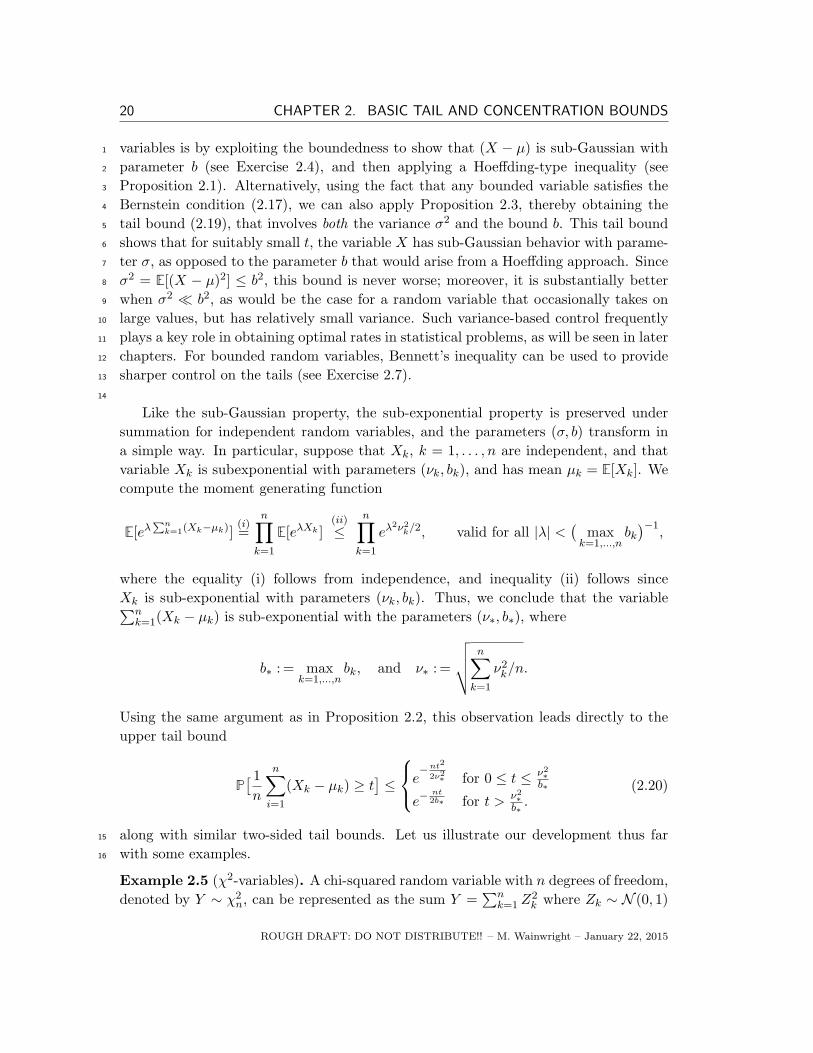
Like the sub-Gaussian property, the sub-exponential property is preserved under
summation for independent random variables, and the parameters (σ, b) transform in
a simple way. In particular, suppose that Xk, k = 1, . . . , n are independent, and that
variable Xk is subexponential with parameters (νk, bk), and has mean µk = E[Xk]. We
compute the moment generating function
E[eλ∑n
k=1(Xk−µk)](i)=
n∏
k=1
E[eλXk ](ii)
≤n∏
k=1
eλ2ν2k/2, valid for all |λ| <
(max
k=1,...,nbk)−1
,
where the equality (i) follows from independence, and inequality (ii) follows since
Xk is sub-exponential with parameters (νk, bk). Thus, we conclude that the variable∑nk=1(Xk − µk) is sub-exponential with the parameters (ν∗, b∗), where
b∗ : = maxk=1,...,n
bk, and ν∗ : =
√√√√n∑
k=1
ν2k/n.
Using the same argument as in Proposition 2.2, this observation leads directly to the
upper tail bound
P[ 1n
n∑
i=1
(Xk − µk) ≥ t]≤
e−nt2
2ν2∗ for 0 ≤ t ≤ ν2∗b∗
e−nt2b∗ for t > ν2∗
b∗.
(2.20)
along with similar two-sided tail bounds. Let us illustrate our development thus far15
with some examples.16
Example 2.5 (χ2-variables). A chi-squared random variable with n degrees of freedom,
denoted by Y ∼ χ2n, can be represented as the sum Y =
∑nk=1 Z
2k where Zk ∼ N (0, 1)
ROUGH DRAFT: DO NOT DISTRIBUTE!! – M. Wainwright – January 22, 2015

SECTION 2.1. CLASSICAL BOUNDS 21
are i.i.d. variates. As discussed in Example 2.4, the variable Z2k is sub-exponential with
parameters (2, 4). Consequently, since the variables Zk, k = 1, 2, . . . , n are independent,
the χ2-variate Y is sub-exponential with parameters (σ, b) = (2√n, 4), and the preceding
discussion yields the two-sided tail bound
P
[∣∣ 1n
n∑
k=1
Z2k − 1
∣∣ ≥ t
]≤ 2e−nt
2/8, for all t ∈ (0, 1). (2.21)
♣ 1
The concentration of χ2-variables plays an important role in the analysis of procedures 2
based on taking random projections. A classical instance of the random projection 3
method is the Johnson-Lindenstrauss analysis of metric embedding. 4
5
Example 2.6 (Johnson-Lindenstrauss embedding). As one application of χ2-concentration,
consider the following problem. Suppose that we are given m data points u1, . . . , umlying in R
d. If the data dimension d is large, then it might be too expensive to store
the data set. This challenge motivates the design of a mapping F : Rd → R
n with
n≪ d that preserves some “essential” features of the data set, and then store only the
projected data set F (u1), . . . , F (um). For example, since many algorithms are based
on pairwise distances, we might be interested in a mapping F with the guarantee that
for all pairs (ui, uj), we have
(1− δ) ‖ui − uj‖22 ≤ ‖F (ui)− F (uj)‖22 ≤ (1 + δ)‖ui − uj‖22, (2.22)
for some tolerance δ ∈ (0, 1). Of course, this is always possible if the projected dimension 6
n is large enough, but the goal is to do it with relatively small n. 7
Constructing such a mapping that satisfies the condition (2.22) with high prob- 8
ability turns out to be straightforward as long as the projected dimension satisfies 9
n = Ω( 1δ2
logm). Observe that the projected dimension is independent of the ambient 10
dimension d, and scales only logarithmically with the number of data points m. 11
The construction is probabilistic: first form a random matrix X ∈ Rn×d filled with
independent N (0, 1) entries, which defines a linear mapping F : Rd → R
n via u 7→Xu/
√n. We now verify that F satisfies condition (2.22) with high probability. Let
Xi ∈ Rd denote the ith row of X, and consider some fixed u 6= 0. Since Xi is a standard
normal vector, the variable 〈Xi, u/‖u‖2〉 follows a N (0, 1) distribution, and hence the
quantity
Y : =‖Xu‖22‖u‖22
=n∑
i=1
〈Xi, u/‖u‖2〉2,
follows a chi-squared distribution with n degrees of freedom, using the independence of
ROUGH DRAFT: DO NOT DISTRIBUTE! – M. Wainwright – January 22, 2015

22 CHAPTER 2. BASIC TAIL AND CONCENTRATION BOUNDS
the rows. Therefore, applying the tail bound (2.21), we find that
P
[∣∣‖Xu‖22
n ‖u‖22− 1
∣∣ ≥ δ
]≤ 2e−nδ
2/8 for all δ ∈ (0, 1).
Re-arranging and recalling the definition of F yields the bound
P
[‖F (u)‖22‖u‖22
/∈ [(1− δ), (1 + δ)]
]≤ 2e−nδ
2/8, for any fixed 0 6= u ∈ Rd.
Noting that there are at most(m2
)distinct pairs of data points, we apply the union
bound to conclude that
P
[‖F (ui − uj)‖22‖ui − uj‖22
/∈ [(1− δ), (1 + δ)] for some ui 6= uj]≤ 2
(m
2
)e−nδ
2/8.
For any ǫ ∈ (0, 1) and m ≥ 2, this probability can be driven below ǫ by choosing1
n > 16δ2
log(m/ǫ). ♣2
As a useful summary, the following theorem provides several equivalent characteri-3
zations of sub-exponential variables:4
5
Theorem 2.2 (Equivalent characterizations of sub-exponential variables). For a zero-
mean random variable X, the following statements are equivalent:
(I) There are non-negative numbers (ν, b) such that
E[eλX ] ≤ eν2λ2
2 for all |λ| < 1b . (2.23)
(II) There is a positive number c0 > 0 such that E[eλX ] <∞ for all |λ| ≤ c0.
(III) There are constants c1, c2 > 0 such that
P[|X| ≥ t] ≤ c1 e−c2 t for all t > 0. (2.24)
(IV) The quantity γ : = supk≥2
[E[Xk]k!
]1/kis finite.
6
7
8
See Appendix B for the proof of this claim.9
ROUGH DRAFT: DO NOT DISTRIBUTE!! – M. Wainwright – January 22, 2015

SECTION 2.1. CLASSICAL BOUNDS 23
2.1.4 Some one-sided results 1
Up to this point, we have focused on two-sided forms of Bernstein’s condition, which 2
then yields to bounds on both the upper and lower tails. As we have seen, one sufficient 3
condition for Bernstein’s condition to hold is an absolute bound, say |X| ≤ b almost 4
surely. Of course, if such a bound only holds in a one-sided way, it is still possible to 5
derive one-sided bounds. In this section, we state and prove one such result. 6
7
Proposition 2.4 (One-sided Bernstein’s inequality). If X ≤ b almost surely, then
E[eλ(X−E[X])] ≤ exp( λ2
2 E[X2]
1− bλ3
)for all λ ∈ [0, 3/b). (2.25)
Consequently, given n independent random variables with Xi ≤ b almost surely, we
have
P[ n∑
i=1
(Xi − E[Xi]) ≥ nδ]≤ exp
(− nδ2
1n
∑ni=1 E[X2
i ] +bδ3
). (2.26)
8
9
10
Of course, if a random variable is bounded from below, then the same result can be
used to derive bounds on its lower tail; we simply apply the bound (2.26) to the random
variable −X. In the special case of independent non-negative random variables Yi ≥ 0,
we find that
P[ n∑
i=1
(Yi − E[Yi]) ≤ nδ]≤ exp
(− nδ2
2n
∑ni=1 E[Y 2
i ]
). (2.27)
Thus, we see that the lower tail of any non-negative random variable satisfies a bound 11
of the sub-Gaussian type, albeit with the second moment instead of the variance. 12
13
The proof of Proposition 2.4 is quite straightforward given our development thus far. 14
Proof. Let us write E[eλX ] = 1 + λE[X] + 12λ
2E[X2h(λX)], where we have defined the
function h(u) = 2 eu−u−1u2
= 2∑∞
k=2uk−2
k! . Observe that for all x < 0 and x′ ∈ [0, b] and
λ > 0, we have
h(λx) ≤ h(0) ≤ h(λx′) ≤ h(λb).
Consequently, since X ≤ b almost surely, we have E[X2h(λX)] ≤ E[X2]h(λb), and
ROUGH DRAFT: DO NOT DISTRIBUTE! – M. Wainwright – January 22, 2015
24 CHAPTER 2. BASIC TAIL AND CONCENTRATION BOUNDS
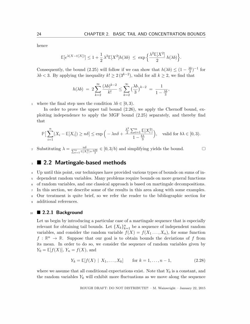
hence
E[eλ(X−E[X])] ≤ 1 +1
2λ2E[X2]h(λb) ≤ exp
λ2E[X2]
2h(λb)
.
Consequently, the bound (2.25) will follow if we can show that h(λb) ≤ (1 − λb3 )
−1 for
λb < 3. By applying the inequality k! ≥ 2 (3k−2), valid for all k ≥ 2, we find that
h(λb) = 2∞∑
k=2
(λb)k−2
k!≤
∞∑
k=2
(λb3
)k−2=
1
1− λb3
,
where the final step uses the condition λb ∈ [0, 3).1
In order to prove the upper tail bound (2.26), we apply the Chernoff bound, ex-
ploiting independence to apply the MGF bound (2.25) separately, and thereby find
that
P[ n∑
i=1
(Xi − E[Xi]) ≥ nδ] ≤ exp(− λnδ +
λ2
2
∑ni=1 E[X2
i ]
1− bλ3
), valid for bλ ∈ [0, 3).
Substituting λ = nδ∑ni=1 E[X
2i ]+
nδb3
∈ [0, 3/b) and simplifying yields the bound.2
2.2 Martingale-based methods3
Up until this point, our techniques have provided various types of bounds on sums of in-4
dependent random variables. Many problems require bounds on more general functions5
of random variables, and one classical approach is based on martingale decompositions.6
In this section, we describe some of the results in this area along with some examples.7
Our treatment is quite brief, so we refer the reader to the bibliographic section for8
additional references.9
2.2.1 Background10
Let us begin by introducing a particular case of a martingale sequence that is especially
relevant for obtaining tail bounds. Let Xknk=1 be a sequence of independent random
variables, and consider the random variable f(X) = f(X1 . . . , Xn), for some function
f : Rn → R. Suppose that our goal is to obtain bounds the deviations of f from
its mean. In order to do so, we consider the sequence of random variables given by
Y0 = E[f(X)], Yn = f(X), and
Yk = E[f(X) | X1, . . . , Xk] for k = 1, . . . , n− 1, (2.28)
where we assume that all conditional expectations exist. Note that Y0 is a constant, and
the random variables Yk will exhibit more fluctuations as we move along the sequence
ROUGH DRAFT: DO NOT DISTRIBUTE!! – M. Wainwright – January 22, 2015

SECTION 2.2. MARTINGALE-BASED METHODS 25
from Y0 to Yn. Based on the intuition, the martingale approach to tail bounds is based
on the telescoping decomposition
Yn − Y0 =n∑
k=1
(Yk − Yk−1
)︸ ︷︷ ︸
Dk
in which the deviation f(X)−E[f(X)] is written as a sum of increments Dknk=1. As we 1
will see, the sequence Yknk=1 is a particular example of a martingale sequence, known 2
as the Doob martingale, whereas the sequence Dknk=1 is an example of a martingale 3
difference sequence. 4
With this example in mind, we now turn to the general definition of a martingale se- 5
quence. Let Fk∞k=1 be a sequence of σ-fields that are nested, meaning that Fk ⊆ Fk+1 6
for all k ≥ 1; such a sequence is known as a filtration. In the Doob martingale described 7
above, the σ-field σ(X1, . . . , Xk) generated by the first k variables plays the role of Fk. 8
Let Yk∞k=1 be a sequence of random variables such that Yk is measurable with re- 9
spect to the σ-field Fk. In this case, we say that Yk∞k=1 is adapted to the filtration 10
Fk∞k=1. In the Doob martingale, the random variable Yk is a measurable function of 11
(X1, . . . , Xk), and hence the sequence is adapted to the filtration defined by the σ-fields. 12
We are now ready to define a general martingale: 13
14
Definition 2.3. Given a sequence Yk∞k=1 of random variables adapted to a filtration
Fk∞k=1, the pair (Yk,Fk)∞k=1 is a martingale if for all k ≥ 1,
E[|Yk|] <∞, and E[Yk+1 | Fk
]= Yk. (2.29)
15
16
17
It is frequently the case that the filtration is defined by a second sequence of random 18
variables Xk∞k=1 via the canonical σ-fields Fk : = σ(X1, . . . , Xk). In this case, we say 19
that Yk∞k=1 is a martingale sequence with respect to Xk∞k=1. The Doob construction 20
is an instance of such a martingale sequence. If a sequence is martingale with respect 21
to itself (i.e., with Fk = σ(Y1, . . . , Yk)), then we say simply that Yk∞k=1 forms a mar- 22
tingale sequence. 23
24
Let us consider some examples to illustrate: 25
Example 2.7 (Partial sums as martingales). Perhaps the simplest instance of a mar-
tingale is provided by considering partial sums of an i.i.d. sequence. Let Xk∞k=1
be a sequence of i.i.d. random variables with mean µ, and define the partial sums
Sk : =∑k
j=1Xj . Defining Fk = σ(X1, . . . , Xk), the random variable Sk is measurable
ROUGH DRAFT: DO NOT DISTRIBUTE! – M. Wainwright – January 22, 2015
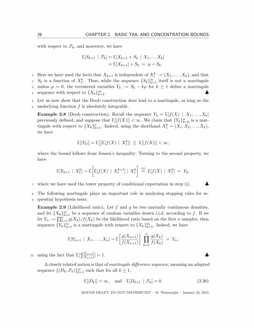
26 CHAPTER 2. BASIC TAIL AND CONCENTRATION BOUNDS
with respect to Fk, and moreover, we have
E[Sk+1 | Fk] = E[Xk+1 + Sk | X1, . . . Xk]
= E[Xk+1] + Sk = µ+ Sk.
Here we have used the facts that Xk+1 is independent of Xk1 : = (X1, . . . , Xk), and that1
Sk is a function of Xk1 . Thus, while the sequence Sk∞k=1 itself is not a martingale2
unless µ = 0, the recentered variables Yk : = Sk − kµ for k ≥ 1 define a martingale3
sequence with respect to Xk∞k=1. ♣4
Let us now show that the Doob construction does lead to a martingale, as long as the5
underlying function f is absolutely integrable.6
Example 2.8 (Doob construction). Recall the sequence Yk = E[f(X) | X1, . . . , Xk]
previously defined, and suppose that E[|f(X)|] <∞. We claim that Yknk=0 is a mar-
tingale with respect to Xknk=1. Indeed, using the shorthand Xk1 = (X1, X2, . . . , Xk),
we have
E[|Yk|] = E[∣∣E[f(X) | Xk
1 |] ≤ E[|f(X)|] <∞,
where the bound follows from Jensen’s inequality. Turning to the second property, we
have
E[Yk+1 | Xk1 ] = E
[E[f(X) | Xk+1
1 ] | Xk1
](i)= E[f(X) | Xk
1 ] = Yk,
where we have used the tower property of conditional expectation in step (i). ♣7
The following martingale plays an important role in analyzing stopping rules for se-8
quential hypothesis tests:9
Example 2.9 (Likelihood ratio). Let f and g be two mutually continuous densities,
and let Xk∞k=1 be a sequence of random variables drawn i.i.d. according to f . If we
let Yn : =∏nk=1 g(Xk)/f(Xk) be the likelihood ratio based on the first n samples, then
sequence Yk∞k=1 is a martingale with respect to Xk∞k=1. Indeed, we have
E[Yn+1 | X1, . . . , Xn] = E
[g(Xn+1)
f(Xn+1)
] n∏
k=1
g(Xk)
f(Xk)= Yn,
using the fact that E[ g(Xn+1)f(Xn+1)
] = 1. ♣10
A closely related notion is that ofmartingale difference sequence, meaning an adapted
sequence (Dk,Fk)∞k=1 such that for all k ≥ 1,
E[|Dk|] <∞, and E[Dk+1 | Fk] = 0. (2.30)
ROUGH DRAFT: DO NOT DISTRIBUTE!! – M. Wainwright – January 22, 2015

SECTION 2.2. MARTINGALE-BASED METHODS 27
As suggested by their name, such difference sequences arise in a natural way from mar-
tingales. In particular, given a martingale (Yk,Fk)∞k=0, let us define Dk = Yk − Yk−1
for k ≥ 1. We then have
E[Dk+1 | Fk] = E[Yk+1 | Fk]− E[Yk | Fk]= E[Yk+1 | Fk]− Yk = 0,
using the martingale property (2.29) and the fact that Yk is measurable with respect to 1
Fk. Thus, for any martingale sequence Yk∞k=0, we have the telescoping decomposition 2
Yn−Y0 =∑n
k=1Dk where Dk∞k=1 is martingale difference sequence. This decomposi- 3
tion plays an important role in our development of concentration inequalities to follow. 4
5
2.2.2 Concentration bounds for martingale difference sequences 6
We now turn to the derivation of concentration inequalities for martingales. These 7
inequalities can be viewed in one of two ways: either as bounds for the difference 8
Yn − Y0, or as bounds for the sum∑n
k=1Dk of the associated martingale difference 9
sequence (MDS). Throughout this section, we present results mainly in terms of mar- 10
tingale differences, with the understanding that such bounds have direct consequences 11
for martingale sequences. Of particular interest to us is the Doob martingale described 12
in Example 2.8, which can be used to control the deviations of a function from its ex- 13
pectation. 14
15
We begin by stating and proving a general Bernstein-type bound for a MDS, based 16
on imposing a sub-exponential condition on the martingale differences. 17
18
Theorem 2.3. Let (Dk,Fk)∞k=1 be a martingale difference sequence, and suppose
that for any |λ| < 1/bk, we have E[eλDk | Fk−1] ≤ eλ2ν2k/2 almost surely. Then
(a) The sum∑n
k=1Dk is sub-exponential with parameters (√∑n
k=1 ν2k , b∗) where
b∗ : = maxk=1,...,n
bk.
(b) Consequently, for all t ≥ 0,
P[|n∑
k=1
Dk| ≥ t]≤
2 e
− t2
2∑n
k=1ν2k if 0 ≤ t ≤
∑nk=1 ν
2k
b∗, and
2 e−t
2 b∗ if t >∑n
k=1 ν2k
b∗.
(2.31)
19
20
Proof. We follow the standard approach of controlling the moment generating function
of∑n
k=1Dk, and then applying the Chernoff bound. Letting λ ∈ (−1/b∗, 1/b∗) be
ROUGH DRAFT: DO NOT DISTRIBUTE! – M. Wainwright – January 22, 2015

28 CHAPTER 2. BASIC TAIL AND CONCENTRATION BOUNDS
arbitrary, conditioning on Fn−1 and applying iterated expectation yields
E[eλ(∑n
k=1Dk
)]= E
[eλ(∑n−1
k=1 Dk
)]E[eλDn | Fn−1]
]
≤ E[eλ
∑n−1k=1 Dk
]eλ
2ν2n/2, (2.32)
where the inequality follows from the stated assumption on Dn. Iterating this procedure1
yields the bound E[eλ
∑nk=1Dk
]≤ eλ
2∑n
k=1 ν2k/2, valid for all |λ| < 1
b∗. By definition, we2
conclude that∑n
k=1Dk is sub-exponential with parameters (√∑n
k=1 ν2k , b∗), as claimed.3
The tail bound (2.31) follows by applying Proposition 2.2.4
In order for Theorem 2.3 to be useful in practice, we need to isolate sufficient and5
easily checkable conditions for the differences Dk to be almost surely sub-exponential6
(or sub-Gaussian when b = +∞). As discussed previously, bounded random variables7
are sub-Gaussian, which leads to the following corollary:8
9
Corollary 2.1 (Azuma-Hoeffding). Let ((Dk,Fk)∞k=1) be a martingale difference
sequence, and suppose that |Dk| ≤ bk almost surely for all k ≥ 1. Then for all t ≥ 0,
P
[|n∑
k=1
Dk| ≥ t
]≤ 2e
− 2t2∑nk=1
b2k . (2.33)
10
11
Proof. Recall the decomposition (2.32) in the proof of Theorem 2.3; from the struc-12
ture of this argument, it suffices to show that E[eλDk | Fk−1] ≤ eλ2b2k/2 a.s. for each13
k = 1, 2, . . . , n. But since |Dk| ≤ bk almost surely, the conditioned variable (Dk | Fk−1)14
is also bounded almost surely, and hence from the result of Exercise 2.4, it is sub-15
Gaussian with parameter at most σ = bk.16
An important application of Corollary 2.1 concerns functions that satisfy a bounded
difference property. In particular, we say that f : Rn → R satisfies the bounded
difference inequality with parameters (L1, . . . , Ln) if for each k = 1, 2, . . . , n,
|f(x1, . . . , xn)− f(x1, . . . , xk−1, x′k, xk+1, . . . , xn)| ≤ Lk for all x, x′ ∈ R
n. (2.34)
For instance, if the function f is L-Lipschitz with respect to the Hamming norm17
dH(x, y) =∑n
i=1 I[xi 6= yi], which counts the number of positions in which x and y18
differ, then the bounded difference inequality holds with parameter L uniformly across19
all co-ordinates.20
21
ROUGH DRAFT: DO NOT DISTRIBUTE!! – M. Wainwright – January 22, 2015

SECTION 2.2. MARTINGALE-BASED METHODS 29
Corollary 2.2 (Bounded differences inequality). Suppose that f satisfies the bounded
difference property (2.34) with parameters (L1, . . . , Ln) and that the random vector
X = (X1, X2, . . . , Xn) has independent components. Then
P[|f(X)− E[f(X)]| ≥ t
]≤ 2e
− 2t2∑nk=1
L2k for all t ≥ 0. (2.35)
1
2
3
Proof. Recalling the Doob martingale introduced in Example 2.8, consider the associ-
ated martingale difference sequence
Dk = E[f(X) | X1, . . . , Xk]− E[f(X) | X1, . . . , Xk−1]. (2.36)
If we define the function g : Rk → R via g(x1, . . . , xk) : = E[f(X) | x1, . . . , xk], the
independence assumption means that we can write
Dk = g(X1, . . . , Xk)− EX′k
[g(X1, . . . , X
′k)]= EX′
k
[g(X1, . . . , Xk)− g(X1, . . . , X
′k)],
where X ′k is an independent copy of Xk. Thus, if we can show that g satisfies the
bounded difference property with parameter Lk in co-ordinate k, then Corollary 2.1
yields the claim. But by independence and the definition of g, for any pair of k-tuples
(x1, . . . , xk) and (x1, . . . , x′k), we can write
g(x1, . . . , xk)− g(x1, . . . , x′k) = EXn
k+1
[f(x1, . . . , xk, Xk+1, . . . , Xn)− f(x1, . . . , x
′k, Xk+1, . . . , Xn)
]
≤ Lk,
using the bounded differences inequality for f . 4
Remark: In the special case when f is L-Lipschitz with respect to the Hamming norm,
Corollary 2.2 implies that
P[|f(X)− E[f(X)]| ≥ t
]≤ 2e−
2t2
nL2 for all t ≥ 0. (2.37)
Let us consider some examples to illustrate. 5
Example 2.10 (U-statistics). Let g : R2 → R be a symmetric function of its arguments.
Given an i.i.d. sequence Xk, k ≥ 1 of random variables, the quantity
U : =1(n2
)∑
j 6=kg(Xj , Xk) (2.38)
ROUGH DRAFT: DO NOT DISTRIBUTE! – M. Wainwright – January 22, 2015

30 CHAPTER 2. BASIC TAIL AND CONCENTRATION BOUNDS
is known as a pairwise U-statistic. For instance, if g(s, t) = |s − t|, then U is an
unbiased estimator of the mean absolute deviation E[|X1 −X2|]. Note that while U is
not a sum of independent random variables, the dependence is relatively weak, and this
is revealed by a martingale analysis. If g is bounded (say ‖g‖∞ ≤ b), then Corollary 2.2
can be used to establish concentration of U around its mean. Viewing U as a function
f(X1, . . . , Xn), for any given co-ordinate k, we have
|f(x1, . . . , xn)− f(x1, . . . , xk−1, x′k, xk+1, . . . , xn)| ≤
1(n2
)∑
j 6=k|g(xj , xk)− g(xj , x
′k)|
≤ (n− 1) (2b)(n2
) =4b
n,
so that the bounded differences property holds with parameter Lk = 4bn in each co-
ordinate. Thus, we conclude that
P[|U − E[U ]| ≥ t
]≤ 2e−
nt2
8b2 .
This tail inequality implies that U is a consistent estimate of E[U ], and also yields finite1
sample bounds on its quality as an estimator. Similar techniques can be used to obtain2
tail bounds on U -statistics of higher order, involving sums over k tuples of variables. ♣3
Example 2.11 (Rademacher complexity). Let εk, k ≥ 1 be an i.i.d. sequence of
Rademacher variables (i.e., taking the values −1,+1 equiprobably, as in Example 2.2).
Given a collection of vectors A ⊂ Rn, define the random variable1
Z : = supa∈A
[ n∑
k=1
akεk
]= sup
a∈A
[〈a, ε〉
]. (2.39)
The random variable Z measures the size of A in a certain sense, and its expectation4
R(A) : = E[Z(A)] is known as the Rademacher complexity of the set A.5
Corollary 2.2 can be used to show that Z(A) is sub-Gaussian. Viewing Z(A) as a
function f(ε1, . . . , εn), we need to bound the maximum change when co-ordinate k is
changed. Let ε′ be an n-vector with ε′j = εj for all j 6= k, and let a ∈ A be arbitrary.
Since f(ε′) ≥ 〈a, ε′〉 for any a ∈ A, we have
〈a, ε〉 − f(ε′) ≤ 〈a, ε− ε′〉 = ak (εk − ε′k) ≤ 2|ak|.
Taking the supremum over A on both sides, we obtain the inequality
f(ε)− f(ε′) ≤ 2 supa∈A
|ak|.
1For the reader concerned about measurability, see the bibliographic discussion in Chapter 4
ROUGH DRAFT: DO NOT DISTRIBUTE!! – M. Wainwright – January 22, 2015

SECTION 2.3. LIPSCHITZ FUNCTIONS OF GAUSSIAN VARIABLES 31
Since the same argument applies with the roles of ε and ε′ reversed, we conclude that f 1
satisfies the bounded difference inequality in co-ordinate k with parameter 2 supa∈A |ak|. 2
Consequently, Corollary 2.2 implies that the the random variable Z(A) is sub-Gaussian 3
with parameter at most 4∑n
k=1 supa∈A
a2k. This sub-Gaussian parameter can be reduced 4
to 4 supa∈A
∑nk=1 a
2k using alternative techniques (see Example 3.2 in Chapter 3). ♣ 5
2.3 Lipschitz functions of Gaussian variables 6
We conclude this chapter with a classical result on the concentration properties of Lip-
schitz functions of Gaussian variables. These functions exhibit a particularly attractive
form of dimension-free concentration. Let us say that function f : Rn → R is L-Lipschitz
with respect to the Euclidean norm ‖ · ‖2 if
|f(x)− f(y)| ≤ L ‖x− y‖2 for all x, y ∈ Rn. (2.40)
7
The following result guarantees that any such function is sub-Gaussian with parameter 8
at most L: 9
10
Theorem 2.4. Let (X1, . . . , Xn) be a vector of i.i.d. standard Gaussian variables,
and let f : Rn → R be L-Lipschitz with respect to the Euclidean norm. Then the
variable f(X)− E[f(X)] is sub-Gaussian with parameter at most L, and hence
P
[∣∣f(X)− E[f(X)]∣∣ ≥ t
]≤ 2e−
t2
2L2 for all t ≥ 0. (2.41)
11
12
Note that this result is truly remarkable: it guarantees that any L-Lipschitz function of 13
a standard Gaussian random vector, regardless of the dimension, exhibits concentration 14
like a scalar Gaussian variable with variance L2. 15
Proof. With the aim of keeping the proof as simple as possible, let us prove a version of 16
the concentration bound (2.41) with a weaker constant in the exponent. (See the bibli- 17
ographic notes for references to proofs of the sharpest results.) We also prove the result 18
for a function that is both Lipschitz and differentiable; since any Lipschitz function is 19
differentiable almost everywhere2, it is then straightforward to extend this result to the 20
general setting. In order to prove this version of the theorem, we begin by stating an 21
auxiliary technical lemma: 22
23
2This fact is a consequence of Rademacher’s theorem.
ROUGH DRAFT: DO NOT DISTRIBUTE! – M. Wainwright – January 22, 2015

32 CHAPTER 2. BASIC TAIL AND CONCENTRATION BOUNDS
Lemma 2.1. Suppose that f : Rn → R is differentiable. Then for any convex function
φ : R → R, we have
E
[φ(f(X)− E[f(X)]
)]≤ E
[φ(π2〈∇f(X), Y 〉
)](2.42)
where X,Y ∼ N (0, In) are standard multivariate Gaussian, and independent.
1
2
We now prove the theorem using this lemma. For any fixed λ ∈ R, applying in-
equality (2.42) to the convex function t 7→ exp(λt) yields
E
[exp
(λf(X)− E[f(X)]
)]≤ E
[exp
(λπ2
n∑
k=1
Yk∂f
∂xk(X)
)]
= EX
[EY
[exp
(λπ2
n∑
k=1
Yk∂f
∂xk(X)
)]]
= EX
[ n∏
k=1
EYk
[exp
(λπ2Yk
∂f
∂xk(X)
)]],
where we have used the independence of X and Y , and the i.i.d. nature of the compo-
nents of Y . Since Yk ∼ N (0, 1), we have
EYk
[exp
(λπ2Yk
∂f
∂xk(X)
)]= exp
(λ2 π2
8
( ∂f∂xk
(X))2),
and hence
E[eλf(X)−E[f(X)]
]≤ E
[e
λ2π2
8‖∇f(X)‖22
]≤ e
18λ2π2 L2
,
where the final inequality follows from the fact that ‖∇f(X)‖2 ≤ L, due to the Lips-
chitz condition on f . We have thus shown that f(X) − E[f(X)] is sub-Gaussian with
parameter at most πL2 , from which the tail bound
P
[∣∣f(X)− E[f(X)]∣∣ ≥ t
]≤ 2 exp
(− 2 t2
π2L2
)for all t ≥ 0
follows from Proposition 2.1.3
4
It remains to prove Lemma 2.1, and we do so via an interpolation method that
exploits the rotation invariance of the Gaussian distribution. For each θ ∈ [0, π/2],
consider the random vector Z(θ) ∈ Rn with components
Zk(θ) : = Xk sin θ + Yk cos θ for k = 1, 2, . . . , n.
ROUGH DRAFT: DO NOT DISTRIBUTE!! – M. Wainwright – January 22, 2015

SECTION 2.3. LIPSCHITZ FUNCTIONS OF GAUSSIAN VARIABLES 33
By the rotation invariance of the Gaussian distribution, we observe that for all θ ∈ [0, π/2],
the pair (Zk(θ), Z′k(θ)) is a jointly Gaussian vector, with zero mean and identity covari-
ance I2. By convexity of φ, we have
EX
[φ(f(X)− EY [f(Y )]
)]≤ EX,Y
[φ(f(X)− f(Y )
)]. (2.43)
Now since Zk(0) = Yk and Zk(π/2) = Xk for all k = 1, . . . , n, we have
f(X)− f(Y ) =
∫ π/2
0
d
dθf(Z(θ))dθ =
∫ π/2
0〈∇f(Z(θ)), Z ′(θ)〉dθ,
and hence
EX
[φ(f(X)− EY [f(Y )]
)]≤ EX,Y
[φ( ∫ π/2
0〈∇f(Z(θ)), Z ′(θ)〉dθ
)]
= EX,Y
[φ( 1
π/2
∫ π/2
0
π
2〈∇f(Z(θ)), Z ′(θ)〉dθ
)]
≤ 1
π/2
∫ π/2
0EX,Y
[φ(π2〈∇f(Z(θ)), Z ′(θ)〉
)]dθ,
where the final step again uses convexity of φ. But since (Zk(θ), Z′k(θ)) ∼ N (0, I2) for
all θ, the expectation does not depend on θ, and so we have
1
π/2
∫ π/2
0EX,Y
[φ(π2〈∇f(Z(θ)), Z ′(θ)〉
)]dθ = E
[φ(π2〈∇f(X), Y 〉
)]
where (X, Y ) are independent standard Gaussian n-vectors. This completes the proof 1
of the bound (2.42). 2
3
Note that the proof makes essential use of various properties specific to the stan- 4
dard Gaussian distribution. However, similar concentration results hold for other non- 5
Gaussian distributions, including the uniform distribution on the sphere and any strictly 6
log-concave distribution (see Chapter 3 for further discussion of such distributions). 7
Without additional structure of the function f (such as convexity), dimension-free con- 8
centration for Lipschitz functions need not hold for an arbitrary sub-Gaussian distribu- 9
tion; see the bibliographic section for further discussion of this fact. 10
Theorem 2.4 is useful for a broad range of problems; let us consider some examples to 11
illustrate. 12
Example 2.12 (χ2 concentration). If Zk ∼ N (0, 1) are i.i.d. standard normal variates,
then Y : =∑n
k=1 Z2k is a chi-squared variate with n degrees of freedom. The most
ROUGH DRAFT: DO NOT DISTRIBUTE! – M. Wainwright – January 22, 2015

34 CHAPTER 2. BASIC TAIL AND CONCENTRATION BOUNDS
direct way to obtain tail bounds for Y is by noting that Z2k is sub-exponential, and
exploiting independence (see Example 2.5). In this example, we pursue an alternative
approach—namely, via concentration for Lipschitz functions of Gaussian variates. In-
deed, defining the variable V =√Y /
√n, we can write V = ‖(Z1, . . . , Zn)‖2/
√n, and
since the Euclidean norm is a 1-Lipschitz function, Theorem 2.4 implies that
P[V ≥ E[V ] + δ] ≤ exp(−nδ2/2) for all δ ≥ 0.
Using concavity of the square root function and Jensen’s inequality, we have
E[V ] ≤√
E[V 2] = 1
n
n∑
i=1
E[Z2k ]1/2
= 1.
Recalling that V =√Y /
√n and putting together the pieces yields
P[Y
n≥ (1 + δ)2] ≤ exp(−nδ2/2) for all δ ≥ 0.
Since (1 + δ)2 = 1 + 2δ + δ2 ≤ 1 + 3δ for all δ ∈ [0, 1], we conclude that
P[Y ≥ n (1 + t)
]≤ exp(−nt2/18) for all t ∈ [0, 3], (2.44)
where we have made the substitution t = 3δ. It is worthwhile comparing this tail1
bound to those that can be obtained by using the fact that each Z2k is sub-exponential,2
as discussed in Example 2.5. ♣3
Example 2.13 (Order statistics). Given a random vector (X1, X2, . . . , Xn), its order
statistics are obtained by re-ordering the samples in a non-increasing manner—namely
as
X(1) ≥ X(2) ≥ . . . ≥ X(n−1) ≥ X(n). (2.45)
As particular cases, we have X(1) = maxk=1,...,nXk and X(n) = mink=1,...,nXk. Given
another random vector (Y1, . . . , Yn), it can be shown that |X(k) − Y(k)| ≤ ‖X − Y ‖2 for
all k = 1, . . . , n, so that each order statistic is a 1-Lipschitz function. (We leave the
verification of this inequality as an exercise for the reader.) Consequently, when X is a
Gaussian random vector, Theorem 2.4 implies that
P[|X(k) − E[X(k)]| ≥ δ] ≤ 2e−δ2
2 for all δ ≥ 0.
♣4
Example 2.14 (Gaussian complexity). This example is closely related to our earlier
discussion of Rademacher complexity in Example 2.11. Let wknk=1 be an i.i.d. sequence
ROUGH DRAFT: DO NOT DISTRIBUTE!! – M. Wainwright – January 22, 2015

SECTION 2.3. LIPSCHITZ FUNCTIONS OF GAUSSIAN VARIABLES 35
of N (0, 1) variables. Given a collection of vectors A ⊂ Rn, define the random variable3
Z : = supa∈A
[ n∑
k=1
akwk
]= sup
a∈A〈a, w〉. (2.46)
As with the Rademacher complexity, the variable Z = Z(A) is one way of measuring
the size of the set A, and will play an important role in later chapters. Viewing Z as
a function f(w1, . . . , wn), let us verify that f is Lipschitz (with respect to Euclidean
norm) with parameter supa∈A ‖a‖2. Let w,w′ ∈ Rn be arbitrary, and let a∗ ∈ A be
any vector that achieves the maximum defining f(w). Following the same argument as
Example 2.11, we have the upper bound
f(w)− f(w′) ≤ 〈a∗, w − w′〉 ≤ W(A) ‖w − w′‖2.
where W(A) = supa∈A ‖a‖2 is the Euclidean width of the set. The same argument
holds with the roles of w and w′ reversed, and hence |f(w)− f(w′)| ≤ W(A) ‖w − w′‖2.Consequently, Theorem 2.4 implies that
P[|Z − E[Z]| ≥ δ] ≤ 2 exp
(− δ2
2W2(A)
). (2.47)
♣ 1
Example 2.15 (Gaussian chaos variables). As a generalization of the previous example,
let Q ∈ Rn×n be a symmetric matrix, and let w, w be independent zero-mean Gaussian
random vectors with covariance matrix In. The random variable
Z : =n∑
i,j=1
Qijwiwj
is known as a (decoupled) Gaussian chaos. By the independence of w and w, we have 2
E[Z] = 0, so it is natural to seek on a tail bound on the event |Z| ≥ t. 3
Conditioned on w, the variable (Z | w) is a zero-mean Gaussian variable with
variance wTQ2w, and consequently, we have the tail bound
P[|Z| ≥ δ | w] ≤ 2e− δ2
2wTQ2w . (2.48)
Let us now bound the random variable Y = ‖Qw‖2. It is a Lipschitz function of the
Gaussian vector w, with Lipschitz constant given by the operator norm |||Q|||op = sup‖u‖2=1
‖Qu‖2.
Moreover, by Jensen’s inequality, we have E[Y ] ≤√
E[wTQ2w] = |||Q|||F. Putting to-
3For measurability concerns, see the bibliographic discussion in Chapter 4.
ROUGH DRAFT: DO NOT DISTRIBUTE! – M. Wainwright – January 22, 2015

36 CHAPTER 2. BASIC TAIL AND CONCENTRATION BOUNDS
gether the pieces yields the tail bound
P[‖Qw‖2 ≥ |||Q|||F + t
]≤ 2 exp
(− t2
2|||Q|||2op).
Setting t2 = 4δ|||Q|||op and simplifying yields
P[wTQT w ≥ 2|||Q|||2F + 2δ|||Q|||op
]≤ 2 exp
(− 2δ
|||Q|||op).
Putting together the pieces, we find that
P[|Z| ≥ δ] ≤ 2 exp(− δ2
4 |||Q|||2F + 4δ|||Q|||op)+ 2 exp
(− 2δ
|||Q|||op)
≤ 4 exp(− δ2
4 |||Q|||2F + 4δ|||Q|||op).
We have thus shown that the Gaussian chaos variable satisfies a sub-exponential tail1
bound. ♣2
Example 2.16 (Singular values of Gaussian random matrices). For integers n > d, let
X ∈ Rn×d be a random matrix with i.i.d. N (0, 1) entries, and let
γ1(X) ≥ γ2(X) ≥ . . . ≥ γd(X) ≥ 0
denote its ordered singular values. By Wielandt’s theorem (see Exercise 8.3), given
another matrix Y ∈ Rn×d, we have
maxk=1,...,d
|γk(X)− γk(Y)| ≤ |||X−Y|||op ≤ |||X−Y|||F. (2.49)
where ||| · |||F denotes the Frobenius norm on matrices—that is, the Euclidean norm on
the matrix viewed as a vector in Rnd. The inequality (2.49) shows that each singular
value γk(X) is a 1-Lipschitz function of the random matrix, so that Theorem 2.4 implies
that for each k = 1, . . . , d, we have
P[∣∣γk(X)− E[γk(X)]
∣∣ ≥ √nδ
]≤ 2e−
nδ2
2 for all δ ≥ 0. (2.50)
Consequently, even though our techniques are not yet powerful enough to characterize3
the expected value of these random singular values, we are guaranteed that the expec-4
tations are representative of the typical behavior. See Chapter 6 for a more detailed5
discussion of the singular values of random matrices. ♣6
ROUGH DRAFT: DO NOT DISTRIBUTE!! – M. Wainwright – January 22, 2015

SECTION 2.3. LIPSCHITZ FUNCTIONS OF GAUSSIAN VARIABLES 37
Appendix A: Equivalent versions of sub-Gaussian variables 1
We establish the equivalence by proving the circle of implications (I) ⇒ (II) ⇒ (III) ⇒ (I), 2
followed by the equivalence (I) ⇐⇒ (IV). 3
4
Implication (I) ⇒ (II): If X is zero-mean and sub-Gaussian with parameter σ, then we
claim that for Z ∼ N (0, 2σ2),
P[X ≥ t]
P[Z ≥ t]≤
√8 e for all t ≥ 0,
showing that X is majorized by Z with constant c =√8 e. On one hand, by the sub-
Gaussianity of X, we have P[X ≥ t] ≤ exp(− t2
2σ2 ) for all t ≥ 0. On the other hand, by
the Mill’s ratio for Gaussian tails, if Z ∼ N (0, 2σ2), then we have
P[Z ≥ t] ≥(√2σ
t− (
√2σ)3
t3)e−
t2
4σ2 for all t > 0. (2.51)
(See Exercise 2.2 for a derivation of this inequality.) We split the remainder of our 5
analysis into two cases. 6
Case 1: First, suppose that t ∈ [0, 2σ]. Since the function Φ(t) = P[Z ≥ t] is decreas-
ing, for all t in this interval,
P[Z ≥ t] ≥ P[Z ≥ 2σ] ≥( 1√
2− 1
2√2
)e−1 =
1√8 e
Since P[X ≥ t] ≤ 1, we conclude that P[X≥t]P[Z≥t] ≤
√8 e for all t ∈ [0, 2σ]. 7
Case 2: Otherwise, we may assume that t > 2σ. In this case, by combining the Mill’s
ratio (2.51) and the sub-Gaussian tail bound and making the substitution s = t/σ, we
find that
supt>2σ
P[X ≥ t]
P[Z ≥ t]≤ sup
s>2
e−s2
4
(√2s − (
√2)3
s3
)
≤ sups>2
s3 e−s2
4
≤√8e,
where the last step follows from a numerical calculation. 8
9
Implication (II) ⇒ (III): Suppose that X is majorized by a zero-mean Gaussian with
ROUGH DRAFT: DO NOT DISTRIBUTE! – M. Wainwright – January 22, 2015

38 CHAPTER 2. BASIC TAIL AND CONCENTRATION BOUNDS
variance τ2. Since X2k is a non-negative random variable, we have
E[X2k] =
∫ ∞
0P[X2k > s]ds =
∫ ∞
0P[|X| > s1/(2k)] ds.
Under the majorization assumption, there is some constant c ≥ 1 such that
∫ ∞
0P[|X| > s1/(2k)]ds ≤ c
∫ ∞
0P[|Z| > s1/(2k)]ds = cE[Z2k],
where Z ∼ N (0, τ2). The polynomial moments of this centered Gaussian variable take
the form,
E[Z2k] =(2k)!
2kk!τ2k, for k = 1, 2, . . ., (2.52)
whence
E[X2k] ≤ cE[Z2k] = c(2k)!
2kk!τ2k ≤ (2k)!
2kk!(c τ)2k, for all k = 1, 2, . . .,
which establishes the moment bound (2.12) with θ = c τ .1
2
Implication (III) ⇒ (I): For each λ ∈ R, we have
E[eλX ] ≤ 1 +∞∑
k=2
|λ|kE[|X|k]k!
, (2.53)
where we have used the fact E[X] = 0 to elminate the term involving k = 1. If X
is symmetric around zero, then all of its odd moments vanish, and by applying our
assumption on θ(X), we obtain
E[eλX ] ≤ 1 +∞∑
k=1
λ2k
(2k)!
(2k)! θ2k
2kk!= e
λ2θ2
2 ,
which shows that X is sub-Gaussian with parameter θ.3
When X is not symmetric, we can bound the odd moments in terms of the even
ones as
E[|λX|2k+1](i)
≤(E[|λX|2k] E[|λX|2k+2]
)1/2 (ii)
≤ 1
2
(λ2kE[X2k] + λ2k+2
E[X2k+2]), (2.54)
where step (i) follows from the Cauchy-Schwarz inequality; and step (ii) follows from
the arithmetic-geometric mean inequality. Applying this bound to the power series
ROUGH DRAFT: DO NOT DISTRIBUTE!! – M. Wainwright – January 22, 2015

SECTION 2.3. LIPSCHITZ FUNCTIONS OF GAUSSIAN VARIABLES 39
expansion (2.53), we obtain
E[eλX ] ≤ 1 +(12+
1
2 · 3!)λ2E[X2] +
∞∑
k=2
( 1
(2k)!+
1
2
[ 1
(2k − 1)!+
1
(2k + 1)!
])λ2kE[X2k]
≤∞∑
k=0
2kλ2kE[X2k]
(2k)!
≤ e(√2λθ)2
2 ,
which establishes the claim. 1
2
(I) ⇒ (IV) : This result is obvious for s = 0. For s ∈ (0, 1), we begin with the
sub-Gaussian inequality E[eλX ] ≤ eλ2σ2
2 , and multiply both sides by e−λ2σ2
2s , thereby
obtaining
E[eλX−λ2σ2
2s]≤ e
λ2σ2 (s−1)2s .
Since this inequality holds for all λ ∈ R, we may integrate both sides over λ ∈ R, using
Fubini’s theorem to justify exchanging the order of integration. On the right-hand side,
we have
∫ ∞
−∞exp
(λ2σ2 (s− 1)
2s
)dλ =
1
σ
√2πs
1− s.
Turning to the left-hand side, for each fixed x ∈ R, we have
∫ ∞
−∞exp
(λx− λ2σ2
2s
)dλ =
√2πs
σe
sx2
2σ2 .
Taking expectations with respect to X, we conclude that
E[e
sX2
2σ2]≤ σ√
2πs
1
σ
√2πs
1− s=
1√1− s
,
which establishes the claim. 3
4
(IV) ⇒ (I): From the bound ex ≤ x+ e9x2/16, we have
E[eλX ] ≤ E[λX] + E
[e
9λ2X2
16
](i)
≤ e9λ2σ2
16 , (2.55)
where inequality (i) is valid for |λ| ≤ 43σ . 5
ROUGH DRAFT: DO NOT DISTRIBUTE! – M. Wainwright – January 22, 2015

40 CHAPTER 2. BASIC TAIL AND CONCENTRATION BOUNDS
It remains to establish a similar upper bound for |λ| > 43σ . Noting that for any
c > 0, the functions f(u) = u2
2c and f∗(v) = cv2
2 are conjugate duals, the Fenchel-Young
inequality implies that
uv ≤ u2
2c+cv2
2, valid for all u, v ∈ R and c > 0.
Applying this inequality with u = λ and v = X yields
E[eλX ] ≤ E[e
λ2σ2
2c+ cX2
2σ2]
= eλ2σ2
2c E[e
cX2
2σ2]
(ii)
≤ eλ2σ2
2c ec/2, (2.56)
where the final inequality follows by Jensen’s inequality, convexity of the exponential,
and the fact that E[X2] = σ2. Taking c = 4/3, then for all |λ| ≥ 43σ , we have
3λ2σ2
8=
λ2σ2
2c=
3λ2σ2
8≥ 2
3=c
2,
so that equation (2.56) implies that
E[eλX ] ≤ eλ2σ2
c = e3λ2σ2
4 for all |λ| ≥ 43σ .
This inequality, combined with the bound (2.55), completes the proof.1
Appendix B: Proof of Theorem 2.22
(II) ⇒ (I): The existence of the moment generating function for |λ| < c0 implies that3
E[eλX ] = 1 + λ2E[X2]2 + o(λ2) as λ→ 0. Moreover, an ordinary Taylor series expansion4
implies that eσ2λ2
2 = 1+ σ2λ2
2 + o(λ2) as λ→ 0. Therefore, as long as σ2 > E[X2], there5
exists some b ≥ 0 such that E[eλX ] ≤ eσ2λ2
2 for all |λ| ≤ 1b .6
7
(I) ⇒ (II): This implication is immediate.8
9
(III) ⇒ (II): For an exponent a > 0 and truncation level T > 0 to be chosen, we have
E[ea|X|
I[|X| ≤ T ]]≤
∫ T
0P[ea|X| ≥ t]dt
≤ 1 +
∫ T
1P[|X| ≥ log t
a]dt.
ROUGH DRAFT: DO NOT DISTRIBUTE!! – M. Wainwright – January 22, 2015

SECTION 2.4. BIBLIOGRAPHIC DETAILS AND BACKGROUND 41
Applying the assumed tail bound, we obtain
E[ea|X|
I[|X| ≤ T ]]≤ 1 + c1
∫ T
1e−
c2 log ta dt
= 1 + c1
∫ T
1t−c2/adt.
For any a ∈ [0, c22 ], we have E[ea|X|
I[|X| ≤ T ]]≤ 1 + c1
2
(1− 1
T
), showing that E[ea|X|] 1
is finite for all a ∈ [0, c22 ]. Since both eaX and e−aX are upper bounded by e|a| |X|, we 2
conclude that E[eaX ] is finite for all |a| ≤ c22 . 3
4
(II) ⇒ (III): By the Chernoff bound with λ = c0/2, we have
P[X ≥ t] ≤ E[ec0X2 ] e−
c0t2
Applying a similar argument to −X, we conclude that P[|X| ≥ t] ≤ c1e−c2t with 5
c1 = E[ec0X/2] + E[e−c0X/2] and c2 = c0/2. 6
7
(II) ⇐⇒ (IV): Since the moment generating function exists in an open interval around
zero, we can consider the power series expansion
E[eλX ] = 1 +∞∑
k=2
λkE[Xk]
k!for all |λ| < a. (2.57)
By definition, the quantity γ(X) is the radius of convergence of this power series, from 8
which the equivalence between (II) and (IV) follows. 9
2.4 Bibliographic details and background 10
Further background and details on tail bounds can be found in various books (e.g., [BK00, 11
Pet95, BLM13, SS91]). Classic papers on tail bounds include those of Bernstein [Ber37], 12
Chernoff [Che52], Bahadur and Ranga [BR60], Bennett [Ben62], Hoeffding [Hoe63] and 13
Azuma [Azu67]. The idea of using the cumulant function to bound the tails of a 14
random variable was first introduced by Bernstein [Ber37], and further developed by 15
Chernoff [Che52], whose name is now frequently associated with the method. The 16
book [SS91] provides a number of more refined results that can be established using 17
cumulant-based techniques. The original work of Hoeffding [Hoe63] gives results both 18
for sums of independent random variables, assumed to be bounded from above, as well 19
as certain types of dependent random variables, including U -statistics. The work of 20
Azuma [Azu67] applies to general martingales that are sub-Gaussian in a conditional 21
sense, as in Theorem 2.3. 22
ROUGH DRAFT: DO NOT DISTRIBUTE! – M. Wainwright – January 22, 2015

42 CHAPTER 2. BASIC TAIL AND CONCENTRATION BOUNDS
The book by Buldygin and Kozachenko [BK00] provides a range of results on sub-1
Gaussian and sub-exponential variates. In particular, Theorems 2.1 and 2.2 are based2
on results from this book. The Orlicz norms, discussed briefly in Exercises 2.18 and 2.19,3
provide an elegant generalization of the sub-exponential and sub-Gaussian families. See4
Section 5.7 and the books [BK00, LT91] for further background on Orlicz norms.5
The Johnson-Lindenstrauss lemma, discussed in Example 2.6, was originally proved6
in the paper [JL84] as an intermediate step in a more general result about Lipschitz7
embeddings. The original proof of lemma was based on random matrices with orthonor-8
mal rows, as opposed to the standard Gaussian random matrix used here. The use of9
random projection for dimension reduction and algorithmic speed-ups has a wide range10
of applications; see the book by Vempala [Vem04] for an overview.11
Tail bounds for U -statistics, as sketched out in Example 2.10, were derived by12
Hoeffding [Hoe63]. The book by de la Pena and Gine [dLPG99] provides more advanced13
results, including extensions to uniform laws for U -processes and decoupling results.14
The bounded differences inequality (Corollary 2.2) and extensions thereof have many15
applications in the study of randomized algorithms as well as random graphs and other16
combinatorial objects. A number of such applications can be found in the survey by17
McDiarmid [McD89], and the book by Boucheron et al. [BLM13].18
Milman and Schechtman [MS86] provide the short proof of Gaussian concentration19
for Lipschitz functions, on which Theorem 2.4 is based. Ledoux [Led01] provides an20
example of a Lipschitz function of i.i.d sequence of Rademacher variables, i.e., taking21
values −1,+1 equiprobably) for which sub-Gaussian concentration fails to hold (c.f.22
p. 128). However, sub-Gaussian concentration does hold for Lipschitz functions of23
bounded random variables with an additional convexity condition; see Section 3.3.5 for24
further details.25
The kernel density estimation problem from Exercise 2.15 is a particular form of26
non-parametric estimation; we return to such problems in Chapters 13 and 14. Al-27
though we have focused exclusively on tail bounds for real-valued random variables,28
there are many generalizations to random variables taking values in Hilbert and other29
function spaces, as considered in Exercise 2.16. The books [LT91, Yur95] contain fur-30
ther background on such results. We also return to consider some versions of these31
bounds in Chapter 14. The Hanson-Wright inequality discussed in Exercise 2.17 was32
proved in the papers [HW71, Wri73]; see the papers [HKZ12, RV13] for more mod-33
ern treatments. The moment-based tail bound from Exercise 2.20 relies on a classi-34
cal inequality due to Rosenthal [Ros70]. Exercise 2.21 outlines the proof of the rate-35
distortion theorem for the Bernoulli source. It is a particular instance of more general36
information-theoretic results that are proved using probabilistic techniques: see the37
book by Cover and Thomas [CT91] for further reading. The Ising model (11.3) dis-38
cussed in Exercise 2.22 has a lengthy history dating back to Ising [Isi25]. The book39
by Talagrand [Tal03] contains a wealth of information on spin glass models and their40
ROUGH DRAFT: DO NOT DISTRIBUTE!! – M. Wainwright – January 22, 2015

SECTION 2.5. EXERCISES 43
mathematical properties. 1
2.5 Exercises 2
Exercise 2.1 (Tightness of inequalities). The Markov and Chebyshev inequalities can- 3
not be improved in general. 4
(a) Provide a random variable X ≥ 0 for which Markov’s inequality (2.1) is met with 5
equality. 6
(b) Provide a random variable Y for which Chebyshev’s inequality (2.2) is met with 7
equality. 8
Exercise 2.2. Let φ(z) = 1√2πe−z
2/2 be the density function of a standard normal 9
Z ∼ N (0, 1) variate. 10
(a) Show that φ′(z) + zφ(z) = 0. 11
(b) Use part (a) to show that
φ(z)
(1
z− 1
z3
)≤ P[Z ≥ z] ≤ φ(z)
(1
z− 1
z3+
3
z5
)for all z > 0. (2.58)
Exercise 2.3. Suppose that X ≥ 0, and that the moment generating function of X
exists in an interval around zero. Given some δ > 0 and integer k = 1, 2, . . ., show that
infk=0,1,2,...
E[|X|k]δk
≤ infλ>0
E[eλX ]
eλδ. (2.59)
Consequently, an optimized bound based on polynomial moments is always at least as 12
good as the Chernoff upper bound. 13
Exercise 2.4. Consider a random variable X with mean µ = E[X], and such that 14
a ≤ X ≤ b almost surely. 15
(a) Defining the function ψ(λ) = logE[eλX ], show that ψ(0) = 0 and ψ′(0) = µ. 16
(b) Show that ψ′′(λ) = Eλ[X2] − (Eλ[X])2, where we define Eλ[f(X)] : = E[f(X)eλX ]
E[eλX ]. 17
Use this fact to obtain an upper bound on supλ∈R |ψ′′(λ)|. 18
(c) Use parts (a) and (b) to establish that X is sub-Gaussian with parameter at most 19
σ = b−a2 . 20
ROUGH DRAFT: DO NOT DISTRIBUTE! – M. Wainwright – January 22, 2015

44 CHAPTER 2. BASIC TAIL AND CONCENTRATION BOUNDS
Exercise 2.5 (Sub-Gaussian bounds and means/variances). Consider a random vari-
able X such that
E[eλX ] ≤ eλ2σ2
2+λµ (2.60)
for all λ ∈ R.1
(a) Show that E[X] = µ.2
(b) Show that var(X) ≤ σ2.3
(c) Suppose that the smallest possible σ satisfying the inequality (2.60) is chosen. Is4
it then true that var(X) = σ2? Prove or disprove.5
Exercise 2.6 (Lower bounds on squared sub-Gaussians). Letting Xini=1 be an i.i.d.
sequence of zero-mean sub-Gaussian variables with parameter σ, consider the normal-
ized sum Zn : = 1n
∑ni=1X
2i . Prove that
P[Zn − E[Zn] ≤ σ2δ
]≤ e−nδ
2/16 for all δ ≥ 0.
This result shows that the lower tail of a sum of squared sub-Gaussian variables behaves6
in a sub-Gaussian way.7
Exercise 2.7 (Bennett’s inequality). (a) Consider a zero-mean random variable such
that |Xi| ≤ b. Prove that
logE[eλXi ] ≤ σ2i λ2eλb − 1− λb
(λb)2
for all λ ∈ R,
where σ2i = var(Xi).8
(b) Given independent random variables X1, . . . , Xn satisfying the condition of part
(a), let σ2 : = 1n
∑ni=1 σ
2i be the average variance. Prove Bennett’s inequality
P[ n∑
i=1
Xi ≥ nδ]≤ exp
− nσ2
b2h( bδσ2
), (2.61)
where h(t) : = (1 + t) log(1 + t)− t for t ≥ 0.9
(c) Show that Bennett’s inequality is at least as good as Bernstein’s inequality.10
Exercise 2.8 (Bernstein and expectations). Consider a non-negative random variable
that satisfies a concentration inequality of the form
P[Z ≥ t] ≤ C e− t2
2(ν2+Bt) (2.62)
ROUGH DRAFT: DO NOT DISTRIBUTE!! – M. Wainwright – January 22, 2015

SECTION 2.5. EXERCISES 45
for positive constants (ν, b) and C ≥ 1. 1
(a) Show that E[Z] ≤ 2ν(√π +
√logC) + 4B(1 + logC). 2
(b) Let Xini=1 be an i.i.d. sequence of zero-mean variables satisfying the Bernstein
condition (2.16). Use part (a) to show that
E[| 1n
n∑
i=1
Xi|]≤ 2σ√
n
(√π +
√log 2
)+
4b
n
(1 + log 2
),
Exercise 2.9 (Sharp upper bounds on binomial tails). Let Xini=1 be an i.i.d. sequence 3
of Bernoulli variables with parameter α ∈ (0, 1/2], and consider the binomial random 4
variable Zn =∑n
i=1Xi. The goal of this exercise is to prove, for any δ ∈ (0, α), a sharp 5
upper bound on the tail probability P[Zn ≤ δn]. 6
(a) Show that P[Zn ≤ δn] ≤ e−nD(δ ‖α), where the quantity
D(δ ‖α) : = δ logδ
α+ (1− δ) log
(1− δ)
(1− α)(2.63)
is the Kullback-Leibler divergence between the Bernoulli distributions with pa- 7
rameters δ and α respectively. 8
(b) Show that the bound from part (a) is strictly better than the Hoeffding bound 9
for all δ ∈ (0, α). 10
Exercise 2.10 (Lower bounds on binomial tails). Let Xini=1 be a sequence of i.i.d. 11
Bernoulli variables with parameter α ∈ (0, 1/2], and consider the binomial random 12
variable Zn =∑n
i=1Xi. In this exercise, we establish a lower bound on the probability 13
P[Zn ≤ δn] for some fixed δ ∈ (0, α), thereby establishing that the upper bound from 14
Exercise 2.9 is tight up to a polynomial pre-factor. Throughout the analysis, we define 15
m = ⌊nδ⌋, the largest integer less than or equal to nδ, and set δ = mn . 16
(a) Prove 1n logP[Zn ≤ δn] ≥ 1
n log(nm
)+ δ logα+ (1− δ) log(1− α). 17
(b) Show that
1
nlog
(n
m
)≥ φ(δ)− log(n+ 1)
n(2.64)
where φ(δ) = −δ log(δ) − (1 − δ) log(1 − δ) is the binary entropy. (Hint: Let Y 18
be binomial random variable with parameters (n, δ) and show that P[Y = ℓ] is 19
maximized when ℓ = m = δn.) 20
ROUGH DRAFT: DO NOT DISTRIBUTE! – M. Wainwright – January 22, 2015
46 CHAPTER 2. BASIC TAIL AND CONCENTRATION BOUNDS
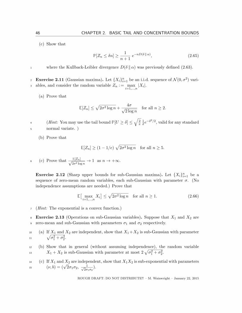
(c) Show that
P[Zn ≤ δn] ≥ 1
n+ 1e−nD(δ ‖α), (2.65)
where the Kullback-Leibler divergence D(δ ‖α) was previously defined (2.63).1
Exercise 2.11 (Gaussian maxima). Let Xini=1 be an i.i.d. sequence of N (0, σ2) vari-2
ables, and consider the random variable Zn : = maxi=1,...,n
|Xi|.3
(a) Prove that
E[Zn] ≤√2σ2 log n+
4σ√2 log n
for all n ≥ 2.
(Hint: You may use the tail bound P[U ≥ δ] ≤√
2π
1δ e
−δ2/2, valid for any standard4
normal variate. )5
(b) Prove that
E[Zn] ≥ (1− 1/e)√2σ2 log n for all n ≥ 5.
(c) Prove that E[Zn]√2σ2 logn
→ 1 as n→ +∞.6
Exercise 2.12 (Sharp upper bounds for sub-Gaussian maxima). Let Xini=1 be a
sequence of zero-mean random variables, each sub-Gaussian with parameter σ. (No
independence assumptions are needed.) Prove that
E[
maxi=1,...,n
Xi
]≤
√2σ2 log n for all n ≥ 1. (2.66)
(Hint: The exponential is a convex function.)7
Exercise 2.13 (Operations on sub-Gaussian variables). Suppose that X1 and X2 are8
zero-mean and sub-Gaussian with parameters σ1 and σ2 respectively.9
(a) If X1 and X2 are independent, show that X1+X2 is sub-Gaussian with parameter10 √σ21 + σ22.11
(b) Show that in general (without assuming independence), the random variable12
X1 +X2 is sub-Gaussian with parameter at most 2√σ21 + σ22.13
(c) IfX1 andX2 are independent, show thatX1X2 is sub-exponential with parameters14
(ν, b) = (√2σ1σ2,
1√2σ1σ2
).15
ROUGH DRAFT: DO NOT DISTRIBUTE!! – M. Wainwright – January 22, 2015

SECTION 2.5. EXERCISES 47
Exercise 2.14 (Concentration around medians and means). Given a scalar random
variable X, suppose that there are positive constants c1, c2 such that
P[|X − E[X]| ≥ t] ≤ c1e
−c2t2 for all t ≥ 0. (2.67)
(a) Prove that var(X) ≤ c1c2. 1
(b) A median mX is any number such that P[X ≥ mX ] ≥ 1/2 and P[X ≤ mX ] ≥ 1/2. 2
Show by example that the median need not be unique. 3
(c) Show that whenever the mean concentration bound (2.67) holds, then for any
median mX ,
P[|X −mX | ≥ t
]≤ c3e
−c4t2 for all t ≥ 0, (2.68)
where c3 : = 4c1 and c4 : =c28 . 4
(d) Conversely, show that whenever the median concentration bound (2.68) holds, 5
then mean concentration (2.67) holds with c1 = 2c3 and c2 =c44 . 6
Exercise 2.15 (Concentration and kernel density estimation). Let X1, X2, . . . , Xn be
i.i.d. samples of random variable with density f on the real line. A standard estimate
of f is the kernel density estimate
fn(x) : =1
nh
n∑
i=1
K(x−Xi
h
),
where K : R → [0,∞) is a kernel function satisfying∫∞−∞K(t)dt = 1, and h > 0 is
a bandwidth parameter. Suppose that we assess the quality of fn using the L1 norm
‖fn − f‖1 : =∫∞−∞ |fn(t)− f(t)|dt. Prove that
P[‖fn − f‖1 ≥ E[‖fn − f‖1] + δ
]≤ e−
nδ2
8 .
Exercise 2.16 (Deviation inequalities in a Hilbert space). Let Xini=1 be a sequence 7
of independent random variables taking values in a Hilbert space H, and suppose that 8
‖Xi‖H ≤ bi almost surely. Consider the real-valued random variable Sn = ‖∑ni=1Xi‖H . 9
(a) Show that for all δ ≥ 0,
P[|Sn − E[Sn]| ≥ nδ] ≤ 2e−
nδ2
8b2 , where b2 = 1n
∑ni=1 b
2i .
ROUGH DRAFT: DO NOT DISTRIBUTE! – M. Wainwright – January 22, 2015

48 CHAPTER 2. BASIC TAIL AND CONCENTRATION BOUNDS
(b) Show that P[Snn ≥ a+ δ] ≤ e−
nδ2
8b2 , where a : =√
1n2
∑ni=1 E[‖Xi‖2H ].1
Exercise 2.17 (Hanson-Wright inequality). Given a positive semidefinite matrixQ ∈ Rn×n,
consider the random variable Z =∑n
i=1
∑nj=1QijXiXj . The Hanson-Wright inequality
guarantees that whenever the random variables Xini=1 are i.i.d. variables with mean
zero, variance 1 and σ-sub-Gaussian, then there are universal constants (c1, c2) such
that
P[Z ≥ trace(Q) + σt
]≤ 2e
−min
c1t|||Q|||op ,
c2t2
|||Q|||2F
, (2.69)
where |||Q|||op and |||Q|||F denote the operator and Frobenius norms, respectively. Prove2
this inequality in the special case Xi ∼ N(0, 1). (Hint: The rotation-invariance of the3
Gaussian distribution and sub-exponential nature of χ2-variates could be useful.)4
Exercise 2.18 (Orlicz norms). Let ψ : R+ → R+ be a strictly increasing convex
function that satisfies ψ(0) = 0. The ψ-Orlicz norm of a random variable X is defined
as
‖X‖ψ : = inft > 0 | E
[ψ(t−1|X|
)]≤ 1
, (2.70)
where ‖X‖ψ is infinite if there is no finite t for which the expectation E[ψ(t−1|X|)]5
exists. For the functions u 7→ uq for some q ∈ [1,∞], then the Orlicz norm is simply6
the usual ℓq-norm ‖X‖q =(E[|X|q]
)1/q. In this exercise, we consider the Orlicz norms7
‖ · ‖ψq defined by the convex functions ψq(u) = exp(uq)− 1, for q ≥ 1.8
(a) If ‖X‖ψq < +∞, show that there exist positive constants c1, c2 such that
P[|X| > t] ≤ c1 exp(−c2tq) for all t > 0. (2.71)
(In particular, you should be able to show that this bound holds with c1 = 2 and9
c2 = ‖X‖−qψq.)10
(b) Suppose that a random variable Z satisfies the tail bound (2.71). Show that11
‖X‖ψq is finite.12
Exercise 2.19 (Maxima of Orlicz variables). Recall the definition of Orlicz norm from
Exercise 2.18. Let Xini=1 be an i.i.d. sequence of zero-mean random variables with
finite Orlicz norm σ = ‖Xi‖ψ. Show that
E[ maxi=1,...,n
|Xi|] ≤ σψ−1(n).
13
ROUGH DRAFT: DO NOT DISTRIBUTE!! – M. Wainwright – January 22, 2015

SECTION 2.5. EXERCISES 49
Exercise 2.20 (Tail bounds under moment conditions). Suppose that Xini=1 are
zero-mean and independent random variables such that, for some fixed integer m ≥ 1,
they satisfy the moment bound ‖Xi‖2m : = (E[X2mi ])
12m ≤ Cm
P[| 1n
n∑
i=1
Xi| ≥ δ]≤ Bm
( 1√nδ
)2mfor all δ > 0,
where Bm is a universal constant depending only on Cm and m.
Hint: You may find the following form of Rosenthal’s inequality to be useful: under
the stated conditions, there is a universal constant Rm such that
E[( n∑
i=1
Xi
)2m] ≤ Rm
n∑
i=1
E[X2mi ] +
( n∑
i=1
E[X2i ])m
.
1
Exercise 2.21 (Concentration and data compression). Let X = (X1, X2, . . . , Xn) be
a vector of i.i.d. Bernoulli variables with parameter 1/2. The goal of lossy data com-
pression is to represent X using a codebook of binary vectors, say z1, . . . , zN, suchthat the rescaled Hamming distortion
δ : = E[
minj=1,...,N
ρH(X, zj)]= E
[min
j=1,...,N
1
n
n∑
i=1
I[Xi 6= zji ]]
is as small as possible. Of course, one can always achieve zero distortion using a 2
codebook with N = 2n codewords, so the goal is to use N = 2Rn codewords for some 3
rate R < 1. In this exercise, we use tail bounds to study the trade-off between the rate 4
R and the distortion δ. 5
(a) Suppose that the rate R is upper bounded as
R < D2(δ ‖ 1/2) = δ log2δ
1/2+ (1− δ) log2
1− δ
1/2.
Show that for any codebook z1, . . . , zN, the probability of achieving distortion 6
δ goes to zero as n goes to infinity. (Hint: Let V j be an 0-1-valued indicator 7
variable for the event ρH(X, zj) ≤ δ, and define V =
∑Nj=1 V
j . The tail bounds 8
from Exercise 2.9 could be useful in bounding the probability P[V ≥ 1].) 9
(b) We now show that if ∆R : = R − D2(δ ‖ 1/2) > 0, then there exists a code- 10
book that achieves distortion δ. In order to do so, consider a random codebook 11
Z1, . . . , ZN, formed by generating each codeword Zj independently, and with 12
all i.i.d. Ber(1/2) entries. Let V j be an indicator for the event ρH(X,Zj) ≤ δ, 13
and define V =∑N
j=1 Vj . 14
ROUGH DRAFT: DO NOT DISTRIBUTE! – M. Wainwright – January 22, 2015

50 CHAPTER 2. BASIC TAIL AND CONCENTRATION BOUNDS
(i) Show that P[V ≥ 1] ≥ (E[V ])2
E[V 2].1
(ii) Use part (i) to show that P[V ≥ 1] → +∞ as n → +∞. (Hint: The tail2
bounds from Exercise 2.10 could be useful.)3
Exercise 2.22 (Concentration for spin glasses). For some positive integer d ≥ 2, con-
sider a collection θjkj 6=k of weights, one for each distinct pair j 6= k of indices in
1, 2, . . . , d. We can then define a probability distribution over the Boolean hypercube
−1,+1d via the mass function
Pθ(x1, . . . , xd) = exp 1√
d
∑
i 6=jθjkxjxk − Fd(θ)
, (2.72)
where the function Fd : R(d2) → R, known as the free energy, is given by
Fd(θ) : = log
( ∑
x∈−1,+1dexp
1√d
∑
j 6=kθjkxjxk
)(2.73)
serves to normalize the distribution. The probability distribution (2.72) was originally4
used to describe the behavior of magnets in statistical physics, in which context it5
is known as the Ising model. Suppose that the weights are chosen as i.i.d. random6
variables, so that equation (2.72) now describes a random family of probability dis-7
tributions. This family is known as the Sherrington-Kirkpatrick model in statistical8
physics.9
(a) Show that Fd is a convex function.10
(b) For any two vectors θ, θ′ ∈ R(d2), show that ‖Fd(θ)− Fd(θ
′)‖2 ≤√d ‖θ − θ′‖2.11
(c) Suppose that the weights are chosen in an i.i.d. manner as θjk ∼ N (0, β2) for
each j 6= k. Use the previous parts and Jensen’s inequality to show that
P
[Fd(θ)
d≥ log 2 +
β2
4+ t
]≤ 2e−βdt
2/2 for all t > 0. (2.74)
Remark: Interestingly, it is known that for any β ∈ [0, 1), this tail bound captures the12
behavior of Fd(θ)/d accurately, in that Fd(θ)d
a.s.−→ log 2 + β2/4. In contrast, for β ≥ 1,13
the behavior of this spin glass model is much more subtle; we refer the reader to the14
bibliographic section for additional reading.15
ROUGH DRAFT: DO NOT DISTRIBUTE!! – M. Wainwright – January 22, 2015