CHAPTER 1

Basic properties of holomorphic functions

Preview of differences between one and severalvariables

For any n ≥ 1, the holomorphy or complex differentiability of a function on a domain inCn implies its analyticity: a holomorphic function has local representations by convergentpower series. This amazing fact was discovered by Cauchy in the years 1830-1840 and ithelps to explain the nice properties of holomorphic functions. On the other hand, when itcomes to integral representations of holomorphic functions, the situation for n ≥ 2 is muchmore complicated than for n = 1: simple integral formulas in terms of boundary valuesexist only for Cn domains that are products of C1 domains. It turns out that functiontheory for a ball in Cn is different from function theory for a “polydisc”, a product ofdiscs.

The foregoing illustrates a constant theme: there are similarities between complexanalysis in several variables and in one variable, but also differences and some of thedifferences are very striking. Thus the subject of analytic continuation presents entirelynew phenomena for n ≥ 2. Whereas every C1 domain carries noncontinuable holomorphicfunctions, there are Cn domains for which all holomorphic functions can be continuedanalytically across a certain part of the boundary (Section 1.9). The problems in Cn

require a variety of new techniques which yield a rich theory.Sections 1.1 – 1.8 deal with simple basic facts, while Sections 1.9 and 1.10 contain

previews of things to come.

NOTATION. The points or vectors of Cn are denoted by

z = (z1, . . . , zn) = x+ iy = (x1 + iy1, . . . , xn + iyn).

For vectors z and w in Cn we use the standard ‘Euclidean’ norm or length and innerproduct,

|z| = ‖z‖ =(

|z1|2 + . . .+ |zn|2)

12

,

(z, w) = 〈z, w〉 = z · w = z1w1 + . . .+ znwn.

Subsets of Cn may be considered as subsets of R2n through the correspondence

(x1 + iy1, . . . , xn + iyn)↔ (x1, y1, . . . , xn, yn) .

Ω will always denote a (nonempty) open subset of the basic underlying space, here Cn. Wealso speak of a domain Ω in Cn, whether it is connected or not. A connected domain willoften be denoted by D if that letter is not required for a derivative.

1.1 Holomorphic functions. Later on we will use the terms ‘analytic’ and ‘holomorphic’interchangeably, but for the moment we will distinguish between them. According to

1

Weierstrass’s definition (about 1870), analytic functions on domains Ω in Cn are locallyequal to sum functions of (multiple) power series [cf. Definition 1.51]. Here we will discussholomorphy.

In order to establish notation, we first review the case of one complex variable. LetΩ be a domain in C ∼ R2. For Riemann (about 1850), as earlier for Cauchy, a complex-valued function

f(x, y) = u(x, y) + iv(x, y) on Ω

provided a convenient way to combine two real-valued functions u and v that occur togetherin applications. [For example, a flow potential and a stream function.] Geometrically,f = u + iv defines a map from one planar domain, Ω, to another. Let us think of adifferentiable map (see below) or of a smooth map (u and v at least of class C1). We fixa ∈ Ω and write

z = x+ iy, z = x− iy,z − a = ∆z = ∆x+ i∆y, z − a = ∆z = ∆x− i∆y.

Then the differential or linear part of f at a is given by

df = df(a) =∂f

∂x(a)∆x+

∂f

∂y(a)∆y

=1

2

(

∂f

∂x+

1

i

∂f

∂y

)

∆z +1

2

(

∂f

∂x− 1

i

∂f

∂y

)

∆z.

In particular dz = ∆z, dz = ∆z. It is now natural to introduce the following symbolicnotation:

1

2

(

∂f

∂x+

1

i

∂f

∂y

)

=∂f

∂z,

1

2

(

∂f

∂x− 1

i

∂f

∂y

)

=∂f

∂z

since it leads to the nice formula

df(a) =∂f

∂z(a)∆z +

∂f

∂z(a)∆z =

∂f

∂zdz +

∂f

∂zdz.

[Observe that ∂f/∂z and ∂f/∂z are not partial derivatives in the ordinary sense – hereone does not differentiate with respect to one variable, while keeping the other variable(s)fixed. However, in calculations, ∂f/∂z and ∂f/∂z do behave like partial derivatives. Theirdefinition is in accordance with the chain rule if one formally replaces the independentvariables x and y by z and z. For a historical remark on the notation, see [Remmert].]

We switch now to complex notation for the independent variables, writingf((z + z)/2, (z − z)/2i) simply as f(z). By definition, the differentiability of the map f ata (in the real sense) means that for all small complex numbers ∆z = z− a = ρeiθ we have

(1a) ∆f(a)def= f(a+ ∆z)− f(a) = df(a) + o(|∆z|) as ∆z → 0.

2

Complex differentiability of such a function f at a requires the existence of

(1b) lim∆z→0

∆f

∆z= lim

∂f

∂z+∂f

∂z

∆z

∆z+ o(1)

.

Note that ∆z/∆z = e−2iθ. Thus for a differentiable map, one has complex differentiabilityat a precisely when the Cauchy-Riemann condition holds at a :

∂f

∂z(a) = 0 or

∂f

∂x=

1

i

∂f

∂y.

[If ∂f/∂z 6= 0, the limit (1b) as ∆z → 0 can not exist.] The representation f = u + ivgives the familiar real Cauchy-Riemann conditions ux = vy , uy = −vx. For the complexderivative one now obtains the formulas

(1c) f ′(a) = lim∆z→0

∆f

∆z=∂f

∂z=∂f

∂x=

1

i

∂f

∂y= ux + ivx = ux − iuy.

Observe that complex differentiability implies differentiability in the real sense.Functions f which possess a complex derivative at every point of a planar domain Ω

are called holomorphic. In particular, analytic functions in C are holomorphic since sumfunctions of power series in z − a are differentiable in the complex sense. On the otherhand, by Cauchy’s integral formula for a disc and series expansion, holomorphy impliesanalyticity, cf. also Section 1.6.

HOLOMORPHY IN THE CASE OF Cn. Let Ω be a domain in Cn ∼ R2n and letf = f(z) = f(z1, . . . , zn) be a complex-valued function on Ω:

(1d) f = u+ iv : Ω→ C.

Suppose for a moment that f is analytic in each complex variable zj separately, sothat f has a complex derivative with respect to zj when the other variables are kept fixed.Then f will satisfy the following Cauchy-Riemann conditions on Ω :

(1e)∂f

∂zj

def=

1

2

(

∂f

∂xj− 1

i

∂f

∂yj

)

= 0, j = 1, . . . , n.

Moreover, the complex partial derivatives ∂f/∂zj will be equal to the corresponding formalderivatives, given by

(1f)∂f

∂zj

def=

1

2

(

∂f

∂xj+

1

i

∂f

∂yj

)

,

cf. (1c).Suppose now that the map f = u + iv of (1d) is just differentiable in the real sense.

[This is certainly the case if f is of class C1.] Then the increment ∆f(a) can be written inthe form (1a), but this time ∆z = (∆z1, . . . ,∆zn) and the differential of f at a is given by

3

df(a) =n∑

1

(

∂f

∂xj(a)∆xj +

∂f

∂yj(a)∆yj

)

=n∑

1

(

∂f

∂zjdzj +

∂f

∂zjdzj

)

.

Thusdf = ∂f + ∂f

[del f and del-bar or d-bar f], where

∂fdef=

n∑

1

∂f

∂zjdzj , ∂f

def=

n∑

1

∂f

∂zjdzj .

With this notation, the Cauchy-Riemann conditions (1e) may be summarized by the singleequation

∂f = 0.

Definition 1.11. A function f on Ω ⊂ Cn to C is called holomorphic if the map f is“differentiable in the complex sense”:

∆f(a) = ∂f(a) + o(|∆z|) as ∆z → 0

at every point a ∈ Ω. In particular a function f ∈ C1(Ω) is holomorphic precisely when itsatisfies the Cauchy-Riemann conditions.

More generally, a function f defined on an arbitrary nonempty set E ⊂ Cn is calledholomorphic, notation

(1g) f ∈ O(E), (also for open E = Ω!)

if f has a holomorphic extension to some open set containing E .The notation O(E) for the class or ring of holomorphic functions on E goes back to

a standard notation for rings, cf. [Van der Waerden] Section 16. The letter O is alsoappropriate as a tribute to the Japanese mathematician Oka, who has made fundamentalcontributions to complex analysis in several variables, beginning about 1935, cf. [Oka].

A function f ∈ O(Ω) will have a complex derivative with respect to each variable zjat every point of Ω, hence by Cauchy’s theory for a disc, f will be analytic in each complexvariable zj separately. A corresponding Cauchy theory for so-called polydiscs will showthat every holomorphic function is analytic in the sense of Weierstrass, see Sections 1.3and 1.6. Thus in the end, holomorphy and analyticity will come to the same thing.

REMARK. The expressions for df , ∂f and ∂f (with variable a) have the appearance ofdifferential forms. First order differential forms

p1dx1 + q1dy1 + . . .+ qndyn or u1dz1 + v1dz1 + . . .+ vndzn,

with dx1, dy1, . . . , dyn or dz1, dz1, . . . , dzn as basis forms (!), will frequently be used as anotational device. Later on we will also need higher order differential forms, cf. Chapter10 for a systematic discussion.

4

1.2 Complex affine subspaces. Ball and polydisc. A single complex linear equation

(2a) c · (z − a)def= c1(z1 − a1) + . . .+ cn(zn − an) = 0 (c 6= 0)

over Cn defines a complex hyperplane V through the point a, just as a single real linearequation over Rn defines a real hyperplane.

EXAMPLE 1.21 (Tangent hyperplanes). Let f be a real C1 function on a domain Ωin Cn ∼ R2n, let a = a′ + ia′′ be a point in Ω and grad f |a 6= 0. Then the equation∆f(a) = f(z)−f(a) = 0 will locally define a real hypersurface S through a. The linearizedequation df(a) = 0 with ∆zj = zj − aj represents the (real) tangent hyperplane to S at a:

0 = df(a) =∑

j

∂f

∂xj(a)(xj − a′j) +

∂f

∂yj(a)(yj − a′′j )

= 2 Re∑

j

∂f

∂zj(zj − aj).

The real tangent hyperplane contains a (unique) complex hyperplane through a, the “com-plex tangent hyperplane” to S at a:

0 = ∂f(a) =∑

j

∂f

∂zj(a)(zj − aj),

cf. exercises 1.4 and 2.9.

A set of k complex linear equations of the form

c(j) · (z − a) = 0, j = 1, . . . , k

defines a complex affine subspace W of Cn, or a complex linear subspace if it passesthrough the origin. Assuming that the vectors c(j) are linearly independent in Cn, Wwill have complex dimension n − k. In the case k = n − 1 one obtains a complex line L(an ordinary complex plane, complex dimension 1). Complex lines are usually given inequivalent parametric form as

(2b) z = a+ wb, or zj = aj + wbj , j = 1, . . . , n,

where a and b are fixed elements of Cn (b 6= 0) and w runs over all of C.

If f ∈ O(Ω) and L is a complex line that meets Ω, the restriction of f to Ω∩L can beconsidered as a holomorphic function of one complex variable. Indeed, if a ∈ Ω∩L and werepresent L in the form (2b), then f(a+wb) will be defined and holomorphic on a certaindomain in C. [Compositions of holomorphic functions are holomorphic, cf. exercise 1.5.]Similarly, if V is a complex hyperplane that meets Ω, the restriction of f to Ω ∩ V can beconsidered as a holomorphic function on a domain in Cn−1.

Open discs in C will be denoted by B(a, r) or ∆(a, r), circles by C(a, r). There aretwo kinds of domains in Cn that correspond to discs in C, namely, balls

5

B(a, r)def= z ∈ Cn : |z − a| < r

and polydiscs (or polycylinders):

∆(a, r) = ∆n(a, r) = ∆(a1, . . . , an; r1, . . . , rn)

def= z ∈ Cn : |z1 − a1| < r1, . . . , |zn − an| < rn= ∆1(a1, r1)× . . .×∆1(an, rn).

Polyradii r = (r1, . . . , rn) must be strictly positive: rj > 0, ∀j. Cartesian products D1 ×. . .×Dn of domains in C are sometimes called polydomains.

Figures 1.1 and 1.2 illustrate the ball B(0, r) and the polydisc ∆(0, r) for the case ofC2 in the plane of absolute values |z1|, |z2|. Every point in the first quadrant representsthe product of two circles. Thus r = (r1, r2) represents the “torus”

T (0, r) = C(0, r1)× C(0, r2).

0 r |z1|

|z2|

0 r1 |z1|

|z2|

r2

r=(r1,r2)

fig 1.1 and 1.2

The actual domains lie in complex 2-dimensional or real 4-dimensional space. The bound-ary of the ball B(0, r) is the sphere S(0, r), the boundary of the “bidisc” ∆ = ∆(0, r) isthe disjoint union

C(0, r1)×∆1(0, r2) ∪ ∆1(0, r1)× C(0, r2) ∪ C(0, r1)× C(0, r2) .

Observe that the boundary ∂∆(0, r) may also be described as the union of closed discs incertain complex lines z1 = c1 and z2 = c2 such that the circumferences of those discs belongto the torus T (0, r). This fact will imply a very strong maximum principle for holomorphicfunctions f on the closed bidisc ∆(0, r). First of all, the absolute value |f | of such afunction must assume its maximum on the boundary ∂∆. This follows readily from themaximum principle for holomorphic functions of one variable: just consider the restrictionsof f to complex lines z2=constant. By the same maximum principle, the absolute value off on the boundary discs of ∆ will be majorized by max |f | on the torus T (0, r). Thus themaximum of |f | on ∆(0, r) is always assumed on the torus T (0, r).

6

By similar considerations, all holomorphic functions on ∆(0, r) = ∆n(0, r) ⊂ Cn

assume their maximum absolute value on the “torus”

T (0, r) = Tn(0, r) = C(0, r1)× . . .× C(0, rn),

a relatively small part (real dimension n) of the whole boundary ∂∆(0, r) (real dimension2n−1). In the language of function algebras, the torus is the distinguished or Shilov bound-ary of ∆(0, r). [It is the smallest closed subset of the topological boundary on which allf under consideration assume their maximum absolute value.] As a result, a holomorphicfunction f on ∆(0, r) will be determined by its values on T (0, r). [If f1 = f2 on T , then... .] Thus mathematical folklore [or functional analysis!] suggests that one can expresssuch a function in terms of its values on T (0, r). We will see below that there is a Cauchyintegral formula which does just that.

For the ball B(0, r) there is no “small” distinguished boundary: all boundary pointsare equivalent. To every point b ∈ S(0, r) there is a holomorphic function f on B(0, r) suchthat |f(b)| > |f(z)| for all points z ∈ B(0, r) different from b, cf. exercise 1.9. Integralrepresentations for holomorphic functions on B(0, r) will therefore involve all boundaryvalues, cf. exercise 1.24 and Chapter 10.

Function theory for a ball in Cn (n ≥ 2) is different from function theory for a polydisc,cf. also [Rudin3,Rudin5]. Indeed, ball and polydisc are holomorphically inequivalent in thefollowing sense: there is no 1− 1 holomorphic map

wj = fj(z1, . . . , zn), j = 1, . . . , n (each fj holomorphic)

of one onto the other [Chapter 5]. This is in sharp contrast to the situation in C, whereall simply connected domains (different from C itself) are holomorphically equivalent [Rie-mann mapping theorem]. In C, function theory is essentially the same for all boundedsimply connected domains.

1.3 Cauchy integral formula for a polydisc. For functions f that are holomorphic ona closed polydisc ∆(a, r), there is an integral representation of Cauchy which extends thewell-known one-variable formula. We will actually assume a little less than holomorphy:

Theorem 1.31. Let f(z) = f(z1, . . . , zn) be continuous on Ω ⊂ Cn and differentiable inthe complex sense with respect to each of the variables zj separately. Then for every closedpolydisc ∆(a, r) ⊂ Ω,

(3a) f(z) =1

(2πi)n

∫

T (a,r)

f(ζ)

(ζ1 − z1) . . . (ζn − zn)dζ1 . . . dζn, ∀z ∈ ∆(a, r)

where T (a, r) is the torus C(a1, r1)× . . .×C(an, rn), with positive orientation of the circlesC(aj , rj).

PROOF. We write out a proof for n = 2. In the first part we only use the complexdifferentiability of f with respect to each variable zj , not the continuity of f .

7

Fix z in ∆(a, r) = ∆1(a1, r1) ×∆1(a2, r2) where ∆(a, r) ⊂ Ω. Then g(w) = f(w, z2)has a complex derivative with respect to w throughout a neighbourhood of the closed disc∆1(a1, r1) in C. The one-variable Cauchy integral formula thus gives

f(z1, z2) = g(z1) =1

2πi

∫

C(a1,r1)

g(w)

w − z1dw =

1

2πi

∫

C(a1,r1)

f(ζ1, z2)

ζ1 − z1dζ1.

For fixed ζ1 ∈ C(a1, r1), the function h(w) = f(ζ1, w) has a complex derivative throughouta neighbourhood of ∆1(a2, r2) in C. Hence

f(ζ1, z2) = h(z2) =1

2πi

∫

C(a2,r2)

h(w)

w − z2dw =

1

2πi

∫

C(a2,r2)

f(ζ1, ζ2)

ζ2 − z2dζ2.

Substituting this result into the first formula, we obtain for f(z1, z2) the repeated integral

(3b) f(z1, z2) =1

(2πi)2

∫

C(a1,r1)

dζ1ζ1 − z1

∫

C(a2,r2)

f(ζ1, ζ2)

ζ2 − z2dζ2.

If we would have started by varying the second variable instead of the first, we wouldhave wound up with a repeated integral for f(z1, z2) in which the order of integration is thereverse. For the applications it is convenient to introduce the (explicit) assumption thatf is continuous, cf. Section 1.6. This makes it possible to rewrite the repeated integral in(3b) as a double integral:

(3c) f(z1, z2) =1

(2πi)2

∫

C(a1,r1)×C(a2,r2)

f(ζ1, ζ2)

(ζ1 − z1)(ζ2 − z2)dζ1dζ2.

Indeed, setting ζ1 = a1 + r1eit1 , ζ2 = a2 + r2e

it2 and

f(ζ1, ζ2)

(ζ1 − z1)(ζ2 − z2)dζ1dζ2 = F (t1, t2)dt1dt2,

we obtain a continuous function F on the closed square region Q = I1× I2, where Ij is theclosed interval −π ≤ tj ≤ π. The integral in (3c) now reduces to the double integral of Fover Q. Since F is continuous on Q, one has the elementary “Fubini” reduction formula

∫

Q

F (t1, t2)dt1dt2 =

∫

I1

dt1

∫

I2

F (t1, t2)dt2

which implies the equality of the integrals in (3c) and (3b).

REMARKS 1.32. In the Theorem, the continuity of f does not have to be postulatedexplicitly. Indeed, in his basic paper of 1906, Hartogs proved that the continuity of ffollows from its complex differentiability with respect to each of the variables zj . Since wewill not need this rather technical result, we refer to other books for a proof, for example[Hormander 1].

8

Cauchy’s integral formula for polydiscs (and polydomains) goes back to about 1840. Itthen took nearly a hundred years before integral representations for holomorphic functionson general Cn domains with (piecewise) smooth boundary began to make their appearance,cf. Chapter 10. Integral representations and their applications continue to be an activearea of research.

In Section 1.6 we will show that functions as in Theorem 1.31 are locally equal to sumfunctions of power series.

1.4 Multiple power series. The general power series in Cn with center a has the form

(4a)∑

α1≥0,...,αn≥0

cα1...αn(z1 − a1)α1 . . . (zn − an)αn .

Here the αj ’s are nonnegative integers and the c’s are complex constants. We will seethat multiple power series have properties similar to those of power series in one complexvariable.

Before we start it is convenient to introduce abbreviated notation. We write α forthe multi-index or ordered n-tuple (α1, . . . , αn) of integers. Such n-tuples are added inthe usual way; the inequality α ≥ β will mean αj ≥ βj , ∀j. In the case α ≥ 0 [that is,αj ≥ 0, ∀j], we also write

α ∈ Nn0 , α! = α1! . . . αn!, |α| = α1 + . . .+ αn (height of α).

One setszα1

1 . . . zαnn = zα, (z1 − a1)α1 . . . (zn − an)αn = (z − a)α,

so that the multiple sum (4a) becomes simply

(4a′)∑

α≥0

cα(z − a)α.

We will do something similar for derivatives, writing

∂

∂zj= Dj ,

∂β1+...+βn

∂zβ1

1 . . . ∂zβnn

= Dβ1

1 . . .Dβnn = Dβ ,

∂

∂zj= Dj .

Returning to (4a), suppose for a moment that the series converges at some point zwith |zj−aj| = rj > 0, ∀j for some (total) ordering of its terms. Then the terms will forma bounded sequence at the given point z [and hence at all points z with |zj − aj| = rj ]:

(4b) |cα| rαn1 . . . rαn

n ≤M < +∞, ∀α ∈ Nn0 .

We will show that under the latter condition, the series (4a) is absolutely convergentthroughout the polydisc ∆(a, r) [for every total ordering of its terms]. The same will betrue for the differentiated series

∑

cαDβ(z − a)α. Thus all these series will have well-

defined sum functions on the polydisc: the sums are independent of the order of the terms.

9

For the proofs it will be sufficient to consider power series with center 0:

(4c)∑

α≥0

cαzα =

∑

cα1...αnzα1

1 . . . zαnn .

Lemma 1.41. Suppose that the terms cαzα form a bounded sequence at the point z = r > 0

(4b). Then the power series (4c) is absolutely convergent throughout the polydisc ∆(0, r).The convergence is uniform on every smaller polydisc ∆(0, λr) with 0 < λ < 1, no matter in

what order the terms are arranged. For every multi-index β ∈ Nn0 and Dβ = Dβ1

1 . . .Dβnn ,

the termwise differentiated series∑

cαDβzα is also absolutely convergent on ∆(0, r) and

uniformly convergent on ∆(0, λr).

0

|z2|

∆(0,λr)

λr

|z1|

r

sx

fig 1.3

PROOF. For z ∈ ∆(0, λr) we have |zj | < λrj , ∀j so that by (4b)

|cαzα| = |cα||zα1

1 | . . . |zαnn | ≤ |cα|λα1rα1

1 . . . λαnrαnn ≤Mλα1 . . . λαn .

On ∆(0, λr) the series (4c) is thus (termwise) majorized by the following convergent (mul-tiple) series of positive constants:

∑

α≥0

Mλα1 . . . λαn = M∑

α1≥0

λα1 . . .∑

αn≥0

λαn = M1

1− λ . . .1

1− λ =M

(1− λ)n.

It follows that the power series (4c) is absolutely convergent [for every total ordering ofits terms] at each point of ∆(0, λr) and finally, at each point of ∆(0, r). Moreover, byWeierstrass’s criterion for uniform convergence, the series will be uniformly convergent on∆(0, λr) for any given order of the terms. [The remainders are dominated by those of themajorizing series of constants.]

We now turn to the final statement in the Lemma. To show the method of proof, itwill be sufficient to consider the simple differential operator D1. It follows from (4b) thatthe differentiated series

∑

cαD1zα =

∑

cαα1zα1−11 zα2

2 . . . zαnn

10

is also majorized by a convergent series of constants on ∆(0, λr), namely, by the series

∑

α≥0

M

r1α1λ

α1−1λα2 . . . λαn =M

r1

(

d

dλ

∑

λα1

)

∑

λα2 . . .∑

λαn =M/r1

(1− λ)n+1.

Thus the differentiated series converges absolutely and uniformly on ∆(0, λr) for eachλ ∈ (0, 1).

Proposition 1.42. Let∑

cαzα be a power series (4c) whose terms are uniformly bounded

at z = r > 0, or suppose only that the series converges throughout the polydisc ∆(0, r) forsome total ordering of the terms, or at least suppose that the terms cαz

α form a boundedsequence at certain points z arbitrarily close to r. Then the series converges absolutelythroughout ∆(0, r), so that the sum

f(z) =∑

α≥0

cαzα, z ∈ ∆(0, r)

is well-defined (the sum is independent of the order of the terms). The sum function f willbe continuous on ∆(0, r) and infinitely differentiable (in the complex sense) with respect toeach of the variables z1, . . . , zn; similarly for the derivatives. The derivative Dβf(z) willbe equal to the sum of the differentiated series

∑

cαDβzα.

PROOF. Choose any λ in (0, 1). Either one of the hypotheses in the Proposition impliesthat the terms cαz

α form a bounded sequence at some point z = s > λr (fig 1.3). Thus wemay apply Lemma 1.41 with s instead of r to obtain absolute and uniform convergence ofthe series on ∆(0, λr). It follows in particular that the sum function f is well-defined andcontinuous on ∆(0, λr) and finally, on ∆(0, r).

We now prove the complex differentiability of f with respect to z1. Fix z2 = b2, . . . ,zn = bn (|bj| < rj). By suitable rearrangement of the terms in our absolutely convergentseries (4c) we obtain

f(z1, b2, . . . , bn) =∑

α1

(

∑

α2,...,αn

cαbα2

2 . . . bαnn

)

zα1

1 , |z1| < r1.

[In an absolutely convergent multiple series we may first sum over some of the indices, thenover the others, cf. Fubini’s theorem for multiple integrals.] A well-known differentiationtheorem for power series in one variable now shows that f(z1, b2, . . . , bn) has a complexderivative D1f for |z1| < r1 which can be obtained by termwise differentiation. Theresulting series for D1f may be rewritten as an absolutely convergent multiple series:

∑

α1

(

∑

α2,...,αn

cαbα2

2 . . . bαnn

)

D1zα1

1 =∑

α

cαD1 (zα1

1 bα2

2 . . . bαnn ) ,

cf. Lemma 1.41. Conclusion: D1f exists throughout ∆(0, r) and D1f(z) =∑

cαD1zα;

similarly for each Dj . Since the new power series converge throughout ∆(0, r), one canrepeat the argument to obtain higher order derivatives.

11

1.5 Analytic functions. Sets of uniqueness. We formalize our earlier rough descrip-tion of analytic functions:

Definition 1.51. A function f on Ω ⊂ Cn to C is called analytic if for every pointa ∈ Ω, there is a polydisc ∆(a, r) in Ω and a multiple power series

∑

cα(z − a)α whichconverges to f(z) on ∆(a, r) for some total ordering of its terms.

It follows from Proposition 1.42 that a power series (4a) for f on ∆ is absolutelyconvergent, hence the order of the terms is immaterial. Proposition 1.42 also implies thefollowing important

Theorem 1.52. Let f(z) be analytic on Ω ⊂ Cn. Then f is continuous on Ω andinfinitely differentiable (in the complex sense) with respect to the variables z1, . . . , zn; thepartial derivatives Dβf are likewise analytic on Ω. If f(z) =

∑

cα(z−a)α on ∆(a, r) ⊂ Ω,then

Dβf(z) =∑

α≥0

cαDβ(z − a)α =

∑

α≥β

cαα!

(α− β)!(z − a)α−β, ∀z ∈ ∆(a, r).

In particular Dβf(a) = cββ!. Replacing β by α, one obtains the coefficient formula

(5a) cα =1

α!Dαf(a) =

1

α1! . . . αn!Dα1

1 . . .Dαnn f(a).

COROLLARIES 1.53. An analytic function f on a domain Ω in Cn has only one (locally)representing power series with center a ∈ Ω. It is the Taylor series, the coefficients are theTaylor coefficients (5a) of f at a.

Analytic functions are holomorphic in the sense of Definition 1.11. [For analytic f onehas ∂f/∂xj = ∂f/∂zj and ∂f/∂yj = i∂f/∂zj, cf. (1c), hence the map f is of class C1 and∂f = 0.]

Theorem 1.54 (uniqueness theorem). Let f1 and f2 be analytic on a connected domainΩ ⊂ Cn and suppose that f1 = f2 throughout a nonempty open subset U ⊂ Ω. (This willin particular be the case if f1 and f2 have the same power series at some point a ∈ Ω.)Then f1 = f2 throughout Ω.

PROOF. Define f = f1 − f2. We introduce the set

E = z ∈ Ω : Dαf(z) = 0, ∀α ∈ Nn0.

E is open. For suppose a ∈ E. There will be a polydisc ∆ = ∆(a, r) ⊂ Ω on which f(z)is equal to the sum of its Taylor series

∑

Dαf(a) · (z − a)α/α!. Hence by the hypothesis,f = 0 throughout ∆. It follows that also Dαf = 0 throughout ∆ for every α, so that∆ ⊂ E.

The complement Ω− E is also open. Indeed, if b ∈ Ω− E then Dβf(b) 6= 0 for someβ. By the continuity of Dβf , it follows that Dβf(z) 6= 0 throughout a neighbourhood of b.Now Ω is connected, hence it is not the union of two disjoint nonempty open sets. SinceE contains U it is nonempty. Thus Ω− E must be empty or Ω = E, so that f ≡ 0.

12

DEFINITION 1.55. A subset E ⊂ Ω in Cn is called a set of uniqueness for Ω [or better,for the class of analytic functions A(Ω)] if the condition “f = 0 throughout E” for analyticf on Ω implies that f ≡ 0 on Ω.

For a connected domain D ⊂ C, every infinite subset E with a limit point in D isa set of uniqueness. [Why? Cf. exercises 1.15, 1.16.] For a connected domain D ⊂ Cn

with n ≥ 2, every ball B(a, r) ⊂ D is a set of uniqueness, but the intersection of Dwith a complex hyperplane c · (z − a) = 0 (c 6= 0) is not a set of uniqueness: think off(z) = c · (z−a) ! One may use the maximum principle for a polydisc [Section 1.2] to showthat if ∆(a, r) ⊂ D, then the torus T (a, r) is a set of uniqueness for D. It is not so muchthe size of a subset E ⊂ D which makes it a set of uniqueness, as well as the way in whichit is situated in Cn, cf. also exercise 1.17.

The counterpart to sets of uniqueness is formed by the zero sets of analytic functions,cf. Section 1.10. Sets of uniqueness (or zero sets) for subclasses of A(Ω), for example, thebounded analytic functions, are not yet well understood, except in very special cases, cf.[Rudin5] for references. Discrete sets of uniqueness for subclasses of A(Ω) are importantfor certain approximation problems, cf. [Korevaar1983].

1.6 Analyticity of the Cauchy integral and consequences. Under the conditions ofTheorem 1.31 the function f represented by the Cauchy integral (3a) will turn out to beanalytic on ∆(a, r). More generally we prove

Theorem 1.61. Let g(ζ) = g(ζ1, . . . , ζn) be defined and continuous on the torus T (a, r) =C(a1, r1)× . . .× C(an, rn). Then the cauchy transform

(6a) f(z) = g(z)def=

1

(2πi)n

∫

T (a,r)

g(ζ)

(ζ1 − z1) . . . (ζn − zn)dζ1 . . . dζn

[where we use positive orientation of the generating circles C(aj, rj) of T (a, r)] is analyticon the polydisc ∆(a, r).

PROOF. By translation we may assume that a = 0. Now taking an arbitrary point b in∆(0, r): |bj | < rj , ∀j, we have to show that f(z) is equal to the sum of a convergentpower series with center b on some polydisc around b. In a situation like the present one,where f(z) is given by an integral with respect to ζ in which z occurs as a parameter, it isstandard procedure to expand the integrand in a power series of the form

∑

dα(ζ)(z− b)αand to integrate term by term.

In order to obtain a suitable series for the integrand, we begin by expanding eachfactor 1/(ζj − zj) around zj = bj :

(6b)1

ζj − zj=

1

ζj − bj − (zj − bj)=

1

ζj − bj1

1− zj−bj

ζj−bj

=∞∑

p=0

(zj − bj)p(ζj − bj)p+1

.

When does this series converge? We must make sure that the ratio |zj − bj|/|ζj − bj|remains less than 1 as ζj runs over the circle C(0, rj). To that end we fix z such that|zj − bj| < rj − |bj|, ∀j (fig 1.4). Then

(6c)|zj − bj||ζj − bj |

≤ |zj − bj|rj − |bj |

def= λj < 1, ∀ζj ∈ C(0, rj).

13

xx

x

ζj

rj

zj

rj - |bj|

bj

0

C(0,rj)

fig 1.4

Thus for ζj running over C(0, rj) the series in (6b) is termwise majorized by the convergentseries of constants

∑

p

Mjλpj =

∑

αj

1

rj − |bj|λαj

j .

There is such a result for each j. Forming the termwise product of the series in (6b)for j = 1, . . . , n, we obtain a multiple series for our integrand:

(6d)

g(ζ)

(ζ1 − z1) . . . (ζn − zn)

=∑

α≥0

g(ζ)

(ζ1 − b1)α1+1 . . . (ζn − bn)αn+1(z1 − b1)α1 . . . (zn − bn)αn .

By (6c) and using the boundedness of g(ζ) on T (0, r), the expansion (6d) is termwise ma-jorized on T (0, r) by a convergent multiple series of constants

∑

αMλα1

1 . . . λαnn . Hence the

series in (6d) is absolutely and uniformly convergent (for any given order of the terms) as ζruns over T (0, r), so that we may integrate term by term. Thus we obtain a representationfor the value f(z) in (6a) by a convergent multiple power series:

(6e) f(z) =∑

α≥0

cα(z − b)α.

Here the coefficients cα [which must also be equal to the Taylor coefficients for f at b] aregiven by the following integrals:

(6f) cα =1

α!Dαf(b) =

1

(2πi)n

∫

T (0,r)

g(ζ)

(ζ1 − b1)α1+1 . . . (ζn − bn)αn+1dζ1 . . . dζn.

The representation will be valid for every z in the polydisc

(6g) ∆(b1, . . . , bn; r1 − |b1|, . . . , rn − |bn|).

14

COROLLARY 1.62 (Osgood’s Lemma). Let f(z) = f(z1, . . . , zn) be continuous on Ω ⊂ Cn

and differentiable in the complex sense on Ω with respect to each variable zj separately.Then f is analytic on Ω.

[By Theorem 1.31, the function f is locally representable as a Cauchy transform. Nowapply Theorem 1.61. Actually, the continuity of f need not be postulated, cf. Remarks1.32.]

Osgood’s lemma shows, in particular, that every holomorphic function is ana-lytic. Thus the class of analytic functions on a domain Ω is the same as the class ofholomorphic functions, A(Ω) = O(Ω). From here on, we will not distinguish between theterms analytic and holomorphic; we usually speak of holomorphic functions.

COROLLARY 1.63 (Convergence of power series throughout polydiscs of holomorphy). Letf be holomorphic on ∆(a, r). Then the power series for f with center a converges to fthroughout ∆(a, r).

[We may take a = 0. If f is holomorphic on (a neighbourhood of) ∆(0, r), it may berepresented on ∆(0, r) by a Cauchy transform over T (0, r). The proof of Theorem 1.61 nowshows that the (unique) power series for f with center b = 0 converges to f throughout∆(0, r), see (6e−g). If f is only known to be holomorphic on ∆(0, r), the precedingargument may be applied to ∆(0, λr), 0 < λ < 1.]

COROLLARY 1.64 (Cauchy integrals for derivatives). Let f be holomorphic on ∆(a, r).Then

Dαf(z) =α!

(2πi)n

∫

T (a,r)

f(ζ)

(ζ1 − z1)α1+1

. . . (ζn − zn)αn+1 dζ1 . . . dζn, ∀z ∈ ∆(a, r).

[By Theorem 1.61, f(z) is equal to a Cauchy transform (6a) on ∆(a, r), with g(ζ) =f(ζ) on T (a, r). Taking a = 0 as we may, the result now follows from (6f) with b = z.Observe that the result corresponds to differentiation under the integral sign in the Cauchyintegral for f (3a). Such differentiation is thus permitted.]

COROLLARY 1.65 (Cauchy inequalities). Let f be holomorphic on ∆(a, r), f(z) =∑

cα(z − a)α. Then

|cα| =|Dαf(a)|

α!≤ M

rα=

M

rα1

1 . . . rαnn,

where M = sup |f(ζ)| on T (a, r).[Use Corollary 1.64 with z = a. Set ζj = aj + rje

itj , j = 1, . . . , n to obtain a boundfor the integral.]

1.7 Limits of holomorphic functions. We will often use yet another consequence ofTheorems 1.31 and 1.61:

Theorem 1.71 (weierstrass). Let fλ, λ ∈ Λ be an indexed family of holomorphicfunctions on Ω ⊂ Cn which converges uniformly on every compact subset of Ω as λ→ λ0.Then the limit function f is holomorphic on Ω. Furthermore, for every multi-index α ∈ Nn

0 ,

Dαfλ → Dαf as λ→ λ0,

15

uniformly on every compact subset of Ω.

In particular, uniformly convergent sequences and series of analytic functions on adomain “may be differentiated term by term”.

PROOF. Choose a closed polydisc ∆(a, r) in Ω. For convenience we write the Cauchyintegral (3a) for fλ in abbreviated form as follows:

(7) fλ(z) = (2πi)−n∫

T (a,r)

fλ(ζ)

ζ − z dζ, z ∈ ∆(a, r).

Keeping z fixed, we let λ→ λ0. Then

fλ(ζ)

ζ − z →f(ζ)

ζ − z , uniformly for ζ ∈ T (a, r).

[The denominator stays away from 0.] Integrating, we conclude that the right-hand side of(7) tends to the corresponding expression with f instead of fλ. The left-hand side tends tof(z), hence the Cauchy integral representation is valid for the limit function f just as forfλ (3a). Theorem 1.61 now implies the analyticity of f on ∆(a, r). Varying ∆(a, r) overΩ, we conclude that f ∈ O(Ω).

Again fixing ∆(a, r) in Ω, we next apply the Cauchy formula for derivatives to f − fλ[Corollary 1.64]. Fixing α and letting λ → λ0, we may conclude that Dα(f − fλ) → 0uniformly on ∆(a, 1

2r). Since a given compact subset E ⊂ Ω can be covered by a finite

number of polydiscs ∆(a, 12r) with a ∈ E and ∆(a, r) ⊂ Ω, it follows that Dαfλ → Dαf

uniformly on E.

COROLLARY 1.72 (Holomorphy theorem for integrals). Let Ω be an open set in Cn andlet I be a compact interval in R, or a product of m such intervals in Rm. Suppose thatthe “kernel” K(z, t) is defined and continuous on Ω × I and that it is holomorphic on Ωfor every t ∈ I. Then the integral

f(z) =

∫

I

K(z, t)dt = lim

s∑

j=1

K(z, τj)m(Ij)

defines a holomorphic function f on Ω. Furthermore, DαzK(z, t) will be continuous on

Ω× I and

Dαf(z) =

∫

I

DαzK(z, t)dt.

Thus, “one may differentiate under the integral sign” here.

For the proof, one may observe the following:(i) The Riemann sums

σ(z, P, τ) =

s∑

j=1

K(z, τj)m(Ij), τj ∈ Ij

16

corresponding to partitionings P of I into appropriate subsets Ij , are holomorphic in z onΩ;

(ii) For a suitable sequence of partitionings, the Riemann sums converge to the integralf(z), uniformly for z varying over any given compact subset E ⊂ Ω.

Indeed, K(z, t) will be uniformly continuous on E × I. We now write the integral asa sum of integrals over the parts Ij of small (diameter and) size m(Ij). It is then easy toshow that the difference between the integral and the approximating sum will be small.

The continuity of DαzK(z, t) on Ω× I may be obtained from the Cauchy integral for

a derivative [Corollary 1.64]. The integral formula for Dαf then follows by differentiationof the limit formula for f(z):

Dαf(z) = lim

s∑

j=1

DαzK(z, τj)m(Ij).

The following two convergence theorems for Cn are sometimes useful. We do notinclude the proofs which are similar to those for the case n = 1, cf. [Narasimhan] or[Rudin2].

THEOREM 1.73 (Montel). A locally bounded family F of holomorphic functions on Ω ⊂Cn is normal, that is, every infinite sequence fk chosen from F contains a subsequencewhich converges throughout Ω and uniformly on every compact subset.

The key observation in the proof is that a locally bounded family of holomorphicfunctions is locally equicontinuous, cf. exercise 1.28. A subsequence fk which convergeson a countable dense subset of Ω will then converge uniformly on every compact subset.

THEOREM 1.74 (Stieltjes-Vitali-Osgood). Let fk be a locally bounded sequence ofholomorphic functions on Ω which converges at every point of a set of uniqueness E forO(Ω). Then the sequence fk converges throughout Ω and uniformly on every compactsubset.

Certain useful approximation theorems for C do not readily extend to Cn. In thisconnection we mention Runge’s theorem on polynomial approximation in C. One maycall Ω ⊂ Cn a Runge domain if every function f ∈ O(Ω) is the limit of a sequence ofpolynomials in z1, . . . , zn which converges uniformly on every compact subset of Ω.

More generally, let V ⊂ W ⊂ C be two domains. Then V is called Runge in W ifevery function f ∈ O(V ) is the limit of a sequence of functions fk ∈ O(W ) which convergesuniformly on every compact subset of V .

THEOREM 1.75 (cf. [Runge] 1885). The Runge domains in C are precisely those opensets, whose complement relative to the extended plane Ce = C ∪ ∞ is connected.

There are several results on Runge domains in Cn, but also open problems, cf.[Hormander1, Range] and especially [Fornæss-Stensønes]. The one-variable theorem pro-vides an extremely useful tool for the construction of counterexamples in complex analysis.

1.8 Open mapping theorem and maximum principle.

Theorem 1.81. Let D ⊂ Cn be a connected domain, f ∈ O(D) nonconstant. Then therange f(D) is open [hence f(D) ⊂ C is a connected domain].

17

This result follows easily from the special case n = 1 by restricting f to a suitablecomplex line. We include a detailed proof because parts of it will be useful later on. Thesituation is more complicated in the case of holomorphic mappings

ζj = fj(z), j = 1, . . . , p, fj ∈ O(D)

from a connected domain D ⊂ Cn to Cp with p ≥ 2. The range of such a map will be openonly in special cases, cf. exercise 1.29 and Section 5.2.

PROOF of Theorem 1.81. It is sufficient to show that for any point a ∈ D and for smallballs B = B(a, r) ⊂ D, the range f(B) contains a neighbourhood of f(a) in C. Bytranslation we may assume that a = 0 and f(a) = 0.

(i) The case n = 1. Since f 6≡ 0, the origin is a zero of f of some finite order s, henceit is not a limit point of zeros of f. Choose r > 0 such that B(0, r)=∆(0, r) belongs to Dand f(z) 6= 0 on C(0, r). Set min|f(z)| on C(0, r) equal to m, so that m > 0. We will showthat for any number c in the disc ∆(0,m), the equation f(z) = c has the same number ofroots in B(0, r) as the equation f(z) = 0, counting multiplicities.

Indeed, by the residue theorem, the number of zeros of f in B(0, r) is equal to

N(f) =1

2πi

∫

C(0,r)+

f ′(z)

f(z)dz.

[Around a zero z0 of f of multiplicity µ, the quotient f ′(z)/f(z) behaves like µ/(z − z0).]We now calculate the number of zeros of f − c in B(0, r):

N(f − c) =1

2πi

∫

C(0,r)

f ′(z)

f(z)− c dz =1

2π

∫ π

−π

f ′(reit)

f(reit)− c reitdt.

By the holomorphy theorem for integrals [Corollary 1.72], N(f − c) will be holomorphic inc on ∆(0,m). Indeed, the final integrand is continuous in (c, t) on ∆(0,m)× [−π, π] and itis holomorphic in c on ∆(0,m) for every t ∈ [−π, π]. Thus since N(f − c) is integer-valued,it must be constant and equal to N(f) ≥ 1.

Final conclusion: f(B) contains the whole disc ∆(0,m).(ii) The case n ≥ 2. Choose B(0, r) ⊂ D. By the uniqueness theorem, f 6≡ 0 in B or

else f ≡ 0 in D. Choose b ∈ B(0, r) such that f(b) 6= 0 and consider the restriction of fto the intersection ∆ of B with the complex line z = wb, w ∈ C. The image f(∆) is thesame as the range of the function

h(w) = f(wb), |w| < r/|b|.

That function is holomorphic and nonconstant: h(0) = 0 6= h(1) = f(b), hence by part (i),the range of h contains a neighbourhood of the origin in C. The same holds a fortiori forthe image f(B).

For functions f as in the Theorem, the absolute value |f | and the real part Re f cannot have a relative maximum at a point a ∈ D. Indeed, any neighbourhood of the pointf(a) in C must contain points f(z) of larger absolute value and of larger real part. One

18

may thus obtain upper bounds for |f | and Re f on D in terms of the boundary values ofthose functions.

Let us define the extended boundary ∂eΩ by ∂Ω if Ω is bounded and by ∂Ω ∪ ∞otherwise; z →∞ will mean |z| → ∞.COROLLARY 1.82 (Maximum principle or maximum modulus theorem). Let Ω be anydomain in Cn, f ∈ O(Ω). Suppose that there is a constant M such that

lim supz→ζ, z∈Ω

|f(z)| ≤M, ∀ζ ∈ ∂eΩ.

Then |f(z)| ≤M throughout Ω. If Ω is connected and f is nonconstant, one has |f(z)| < Mthroughout Ω.

Indeed, if µ = supD |f | would be larger than M for some connected component Dof Ω, then f would be nonconstant on D and µ would be equal to lim |f(zν)| for somesequence zν ⊂ D that can not tend to ∂eΩ. Taking a convergent subsequence we wouldfind that µ = |f(a)| for some point a ∈ D, contradicting the open mapping theorem.

In C, more refined ways of estimating |f | from above depend on the fact that log|f | is asubharmonic function - such functions are majorized by harmonic functions with the sameboundary values. For holomorphic functions f in Cn, log|f | is a so-called plurisubharmonicfunction: its restrictions to complex lines are subharmonic. Plurisubharmonic functionsplay an important role in n-dimensional complex analysis, cf. Chapter 8; their theory isan active subject of research.

1.9 Preview: analytic continuation, domains of holomorphy, the Levi problemand the ∂ equation. Given an analytic function f on a domain Ω ⊂ Cn, we can chooseany point a in Ω and form the power series for f with center a, using the Taylor coefficients(5a). Let U denote the union of all polydiscs ∆(a, r) on which the Taylor series converges.The sum function g of the series will be analytic on U [see Osgood’s criterion 1.62] andit coincides with f around a. Suppose now that U extends across a boundary point b ofΩ (fig 1.5). Then g will provide an analytic continuation of f. It is not required thatsuch a continuation coincide with f on all components of U ∩ Ω.

U'

ax

Ω

fig 1.5The subject of analytic continuation will bring out a very remarkable difference be-

tween the case of n ≥ 2 complex variables and the classical case of one variable. For adomain Ω in the complex plane C and any (finite) boundary point b ∈ ∂Ω, there alwaysexist analytic functions f on Ω which have no analytic continuation across the point b,

19

think of f(z) = 1/(z− b). By suitable distribution of singularities along ∂Ω, one may evenconstruct analytic functions on Ω ⊂ C which can not be continued analytically across anyboundary point; we say that Ω is their maximal domain of existence.

0

r2=|z2|

D

tr D^

r1=|z1|

(1/2,2)

(2,1/2)

S = tr D

fig 1.6However, in Cn with n ≥ 2 there are many domains Ω with the property that all

functions in O(Ω) can be continued analytically across a certain part of the boundary.Several examples of this phenomenon were discovered by Hartogs around 1905. We mentionhis striking spherical shell theorem: For Ω = B(a,R)− B(a, ρ) where 0 < ρ < R, everyfunction in O(Ω) has an analytic continuation to the whole ball B(a,R) [cf. Sections2.8, 3.4]. Another example is indicated in fig 1.6, where D stands for the union of twopolydiscs in C2 with center 0. For every f ∈ O(D) the power series with center 0 convergesthroughout D, but any such power series will actually converge throughout the largerdomain D, thus providing an analytic continuation of f to D [cf. Section 2.4].

Many problems in complex analysis of several variables can only be solved on so-calleddomains of holomorphy; for other problems, it is at least convenient to work with suchdomains. Domains of holomorphy Ω in Cn are characterized by the following property:For every boundary point b, there is a holomorphic function on Ω which has no analyticcontinuation to a neighourhood of b. What this means precisely is explained in Section2.1, cf. also the comprehensive definition in Section 6.1. The following sufficient conditionis very useful in practice: Ω is a domain of holomorphy if for every sequence of points inΩ which converges to a boundary point, there is a function in O(Ω) which is unboundedon that sequence [see Section 6.1]. Domains of holomorphy Ω will also turn out to bemaximal domains of existence: there exist functions in O(Ω) which can not be continuedanalytically across any part of the boundary [Section 6.4].

We will see in Section 6.1 that every convex domain in Cn ∼ R2n is a domain ofholomorphy. All domains of holomorphy have certain (weaker) convexity properties, goingby names such as holomorphic convexity and pseudoconvexity [Chapter 6; fig 1.6 illustratesa pseudoconvex domain D in C2]. For many years it was a major question if all pseudo-convex domains are, in fact, domains of holomorphy (levi problem). The answer is yes[cf. Chapters 7, 11]. Work on the Levi problem has led to many notable developments incomplex analysis.

We mention some problems where domains of holomorphy are important:

HOLOMORPHIC EXTENSION from affine subspaces. Let Ω be a given domain in Cn andlet W denote an arbitrary affine subspace of Cn. If f belongs to O(Ω), the restriction of f

20

to the intersection Ω ∩W will be holomorphic for every choice of W . Conversely, supposeh is some holomorphic function on some intersection Ω ∩ W . Can h be extended to afunction in O(Ω)? This problem turns out to be generally solvable for all affine subspacesW if and only if Ω is a domain of holomorphy [cf. Chapter 7].

SUBTRACTION of NONANALYTIC PARTS. Various problems fall into the followingcategory. One seeks to determine a function h in O(Ω) which satisfies a certain side-condition (S), and it turns out that it is easy to construct a smooth function g on Ω[g ∈ C2(Ω), say] that satisfies condition (S). One then tries to obtain h by subtractingfrom g its “nonanalytic part” u without spoiling (S): h = g − u. What conditions doesthe correction term u have to satisfy? Since h must be holomorphic, it must satisfy theCauchy-Riemann condition ∂h = 0. It follows that umust solve an inhomogeneous problemof the form

(9) ∂u = ∂g on Ω, u : (S0).

[Indeed, h must satisfy condition (S) the same as g, hence u = g − h must satisfy anappropriate zero condition (S0).] Solutions of the global problem (9) do not always exist,but the differential equation has solutions satisfying appropriate growth conditions if Ω is(pseudoconvex or) a domain of holomorphy [Chapter 11]. The spherical shell theorem ofHartogs may be proved by the method of subtracting the nonanalytic part, cf. Chapter 3.

GENERAL ∂ EQUATIONS. The general first order ∂ equation or inhomogeneous Cauchy-Riemann equation on Ω ⊂ Cn has the form

∂u =∑n

1

∂u

∂zjdzj = v =

∑n

1vjdzj

or, written as a system,

∂u/∂zj = vj , j = 1, . . . , n.

The equation is locally solvable whenever the local integrability or compatibility conditions

∂vk/∂zj [= ∂2u/∂zk∂zj = ∂2u/∂zj∂zk] = ∂vj/∂zk

are satisfied, as they are in the case of (9) [cf. Chapter 7]. There are also higher order∂ equations where the unknown is a differential form, not a function. Assuming that thenatural local integrability conditions are satisfied, all ∂ equations are globally solvable onΩ if and only if Ω is a domain of holomorphy, cf. Chapters 11, 12.

COUSIN PROBLEMS: see below.

1.10 Preview: zero sets, singularity sets and the Cousin problems. For holomor-phic functions in C, the best known singularities are the isolated ones: poles and essentialsingularities. However, holomorphic functions in Cn with n ≥ 2 can not have isolatedsingularities. More accurately, it follows from Hartogs’ spherical shell theorem that suchsingularities are removable, cf. Sections 1.9, 2.6.

21

From here on, let Ω be a connected domain in Cn. We suppose first that f is holo-morphic on Ω and not identically zero. In the case n = 1 it is well-known that the zeroset Z(f) = Zf of f is a discrete set without limit point in Ω, cf. exercises 1.15, 1.16.However, for n ≥ 2 a zero set Zf can not have isolated points [1/f can not have isolatedsingularities]. Zf will be a so-called analytic set of complex codimension 1 (complex di-mension n − 1). Example: a complex hyperplane (2a). The local behaviour of zero setswill be studied in Chapter 4.

Certain thin singularity sets are also analytic sets of codimension 1 [Section 4.8].We now describe some related global existence questions, the famous Cousin problems

of 1895 which have had a great influence on the development of complex analysis in Cn.

FIRST COUSIN PROBLEM. Are there meromorphic functions on Ω ⊂ Cn with arbitrarilyprescribed local infinitary behaviour (of appropriate type)?

A meromorphic function f is defined as a function which can locally be represented asa quotient of holomorphic functions. The local data may thus be supplied in the followingway. One is given a covering Uλ of Ω by (connected) open subsets and for each set Uλ,an associated quotient fλ = gλ/hλ of holomorphic functions with hλ 6≡ 0. One wants todetermine a meromorphic function f on Ω which on each set Uλ becomes infinite just likefλ, that is, f − fλ ∈ O(Uλ). Naturally, the data Uλ, fλ must be compatible in the sensethat fλ − fµ ∈ O(Uλ ∩ Uµ) for all λ, µ.

For n = 1 Mittag-Leffler had shown that such a problem is always solvable. Forexample, if Ω is the right half-plane Re z > 0 in C, a meromorphic function f with poleset λ = 1, 2, . . . and such that f(z)− 1/(z − λ) is holomorphic on a neighbourhood of λis provided by the sum of the series

∑∞

λ=1

(

1

z − λ +1

λ

)

.

For n ≥ 2 it turned out that the first Cousin problem is not generally solvable for everydomain Ω in Cn. However, the problem is generally solvable on domains of holomorphy Ω(Oka 1937). The global solution is constructed by patching together local pieces. Thereis a close connection between the solvability of the first Cousin problem and the globalsolvability of a related ∂ equation [Chapters 7, 11]. Oka’s original method has developedinto the important technique of sheaf cohomology (Cartan-Serre 1951-1953, see Chapter 12and cf. [Grauert-Remmert]).

SECOND COUSIN PROBLEM. Are there holomorphic functions f on Ω ⊂ Cn with arbi-trarily prescribed local vanishing behaviour (of appropriate type)?

The data will consist of a covering Uλ of Ω by (connected) open subsets and for eachset Uλ, an associated holomorphic function fλ 6≡ 0. One wants to determine a holomorphicfunction f on Ω which on each set Uλ vanishes just like fλ. Here one must require that onthe intersections Uλ ∩ Uµ, the functions fλ and fµ vanish in the same way, that is, fλ/fµmust be equal to a zero free holomorphic function. The family Uλ, fλ and equivalentCousin-II data determine a so-called divisor D on Ω. The desired function f ∈ O(Ω)must have the local vanishing behaviour given by D. One says that f must have D as adivisor. In the given situation this means that on every set Uλ, the quotient f/fλ must beholomorphic and zero free.

22

For n = 1 Weierstrass had shown that such a problem is always solvable. For example,if Ω is the right half-plane Re z > 0 in C, a holomorphic function f with zero zetλ = 1, 2, . . . and corresponding multiplicities 1 is provided by the infinite product

∏∞

λ=1

(

1− z

λ

)

ez/λ.

For n ≥ 2 the second Cousin problem or divisor problem is not generally solvable,not even if Ω is a domain of holomorphy. General solvability on such a domain requiresan additional condition of topological nature (Oka 1939) which may also be formulated incohomological language (Serre 1953), see Chapter 12. The divisor problem is importantfor algebraic geometry.

From the preceding, the reader should not get the impression that all problems in theCousin I, II area have now been solved. Actually, after the solution of the classical Cousinproblems, the situation for Cn is much like the situation was for one complex variable afterthe work of Mittag-Leffler and Weierstrass. In the case of C, one then turned to muchmore difficult problems such as the determination of holomorphic functions of prescribedgrowth with prescribed zero set, cf. [Boas]. The corresponding problems for Cn are largelyopen, although a start has been made, cf. [Ronkin] and [Lelong-Gruman].

23

Exercises

1.1. Use the definition of holomorphy (1.11) to prove that a holomorphic function onΩ ⊂ Cn has a complex (partial) derivative with respect to each variable zj throughoutΩ.

1.2. Prove that O(Ω) is a ring relative to ordinary addition and multiplication of functions.Which elements have a multiplicative inverse in O(Ω)? Cf. (1g) for the notation.

1.3. (i) Prove that there is exactly one complex line through any two distinct points aand b in Cn.

(ii) Determine a parametric representation for the complex hyperplane c · (z− a) = 0in Cn.

1.4. The real hyperplane V through a = a′ + ia′′ in Cn ∼ R2n with normal direction(α1, β1, . . . , αn, βn) is given by the equation

α1(x1 − a′1) + β1(y1 − a′′1) + . . .+ αn(xn − a′n) + βn(yn − a′′n) = 0.

Show that V can also be represented in the form

Re c · (z − a) = 0.

Verify that a real hyperplane through a in Cn contains precisely one complex hyper-plane through a.

1.5. Prove that the composition of differentiable maps ζ = f(w) : D ⊂ Cp ∼ R2p to Cand w = g(z) : Ω ⊂ Cn ∼ R2n to D is differentiable, and that

∂(f g)

∂zj=

p∑

k=1

∂f

∂wk(g)

∂gk∂zj

+∂f

∂wk(g)

∂gk∂zj

, j = 1, . . . , n.

Deduce that for holomorphic f and g (that is, f and g1, . . . , gp holomorphic), thecomposite function f g is also holomorphic.

1.6. Let f be holomorphic on Ω ⊂ Cn and let V be a complex hyperplane intersectingΩ. Prove that the restriction of f to the intersection Ω ∩ V may be considered as aholomorphic function on an open set in Cn−1.

1.7. Analyze the boundary of the polydisc ∆3(0, r). Then use the maximum principle forthe case of one complex variable to prove that all holomorphic functions f on ∆3(0, r)assume their maximum absolute value on T3(0, r).

1.8. Let b be an arbitrary point of the torus T (0, r) ⊂ Cn. Determine a holomorphicfunction f on the closed polydisc ∆(0, r) for which |f | assumes its maximum only atb. [First take n = 1, then n ≥ 2.]

1.9. Let b be an arbitrary point of the sphere S(0, r) ⊂ Cn. Prove that for f(z) = b · z,one has |f(z)| ≤ r2 on B(0, r) with equality if and only if z = eiθb for some θ ∈ R.Deduce that for f(z) = b · z + 1, one has |f(z)| < |f(b)| throughout B(0, r)− b.

24

1.10. Let f be holomorphic on ∆(0, r). Apply Cauchy’s integral formula to g = f p and letp→∞ in order to verify that

|f(z)| ≤ supT (0,r)|f(ζ)|, ∀z ∈ ∆(0, r).

1.11. Extend the Cauchy integral formula for polydiscs to polydomains D = D1× . . .×Dn,where Dj ⊂ C is the interior of a piecewise smooth simple closed curve Γj , j =1, . . . , n.

1.12. Represent the following functions by double power series with center 0 ∈ C2 anddetermine the respective domains of convergence (without grouping the terms of thepower series):

1

(1− z1)(1− z2),

1

1− z1z2,

1

1− z1 − z2,

ez1

1− z2.

1.13. Suppose that the power series∑

cα(z−a)α converges throughout the open set U ⊂ Cn.Prove that(i) the series is absolutely convergent on U ;

(ii) the convergence is locally uniform on U for any given order of the terms;(iii) the sum function is holomorphic on U.

1.14. Let f be analytic on a connected domain Ω ⊂ Cn and such that Dαf(a) = 0 for acertain point a ∈ Ω and all α ∈ N0. Prove that f ≡ 0.

1.15. Let f be analytic on a connected domain D ⊂ C and f 6≡ 0. Verify that for every pointa ∈ D there is an integer m ≥ 0 such that f(z) = (z − a)mg(z), with g analytic on Dand zero free on a neighbourhood of a. Show that in C2, there is no correspondinggeneral factorization f(z) = (z1 − a1)m1(z2 − a2)m2g(z), with g zero free around a.

1.16. Let D be a connected domain in C and zk a sequence of distinct points in D withlimit a ∈ D. Verify that an analytic function f on D which vanishes at the points zkmust be identically zero. Devise possible extensions of this result to C2.

1.17. For the unit bidisc ∆(0, 1) = ∆1(0, 1)×∆1(0, 1) in C2, a small planar domain around0 may be a set of uniqueness, depending on what plane it lies in. Taking 0 < r < 1

2,

show that the square

E1 = x+ iy ∈ ∆ : |x1| < r, |x2| < r, y1 = y2 = 0

is a set of uniqueness for the analytic functions f on ∆, whereas the square

E2 = x+ iy ∈ ∆ : |x1| < r, |y1| < r, x2 = y2 = 0

is not. [One may use a power series, or one may begin by considering f(z1, x2) withfixed x2 ∈ (−r, r).]

25

1.18. Does the Cauchy transform (6a) define an analytic function on the exterior of theclosed polydisc ∆(a, r)? Compare the cases n = 1 and n = 2.

1.19. Let f(x1 + iy1, . . . , xn + iyn) be of class C1 on Ω ⊂ Cn ∼ R2n as a function ofx1, y1, . . . , xn, yn and such that ∂f ≡ 0. Prove that f(z) = f(z1, . . . , zn) is analyticon Ω.

1.20. Let D be a connected domain in Cn. Prove that the ring O(D) has no zero divisors:if fg ≡ 0 with f, g ∈ O(D) and f(a) 6= 0 at a point a ∈ D, then g ≡ 0.

1.21. (Extension of Liouville’s theorem) Prove that a bounded holomorphic function on Cn

must be constant.

1.22. Let f be holomorphic on a connected domain D of the form Cn − E where n ≥ 2and E is compact. Suppose that f(z) remains bounded as |z| → ∞. Prove thatf = constant (so that the “singularity set” E is removable). [Consider the restrictionsof f to suitable complex lines.]

1.23. Let f be holomorphic on the closed polydisc ∆(0, r) ⊂ C2. Prove the following meanvalue properties:

f(0) =1

m2(T )

∫

T (0,r)

f(ζ)dm2(ζ) =1

m3(∂∆)

∫

∂∆

f(ζ)dm3(ζ).

Here dmj denotes the appropriate area or volume element. [Since the circles ζ1 =r1e

it1 , ζ2 = constant and ζ1 = constant, ζ2 = r2eit2 on T (0, r) intersect at right

angles, the area element dm2(ζ) is simply equal to the product of the elements ofarc length, r1dt1 and r2dt2. Again by orthogonality, the volume element dm3(ζ) ofC(0, r1)×∆1(0, r2) may be represented in the form r1dt1 · ρdρdt2, etc.]

1.24. Prove that holomorphic functions f on the closed unit ball B ⊂ C2 have the followingmean value property:

f(0) =1

m3(S)

∫

S

f(ζ)dm3(ζ), S = ∂B.

[S is a union of tori T (0, r) with r1 = ρ, r2 = (1 − ρ2)12 . The parametrization ζ1 =

ρeit1 , ζ2 = (1 − ρ2)12 eit2 introduces orthogonal curvilinear coordinates on S and

dm3(ζ) = ρdt1(1− ρ2)12 dt2dρ.]

Used in conjunction with suitable holomorphic automorphisms of the ball, this meanvalue property gives a special integral representation for f(z) on B in terms of theboundary values of f on S, cf. exercise 10.28.

1.25. Let f(z1, z2) be continuous on the closed polydisc ∆2(a, r) and holomorphic on theinterior. Take ζ1 on C(a1, r1). Now use Weierstrass’s limit theorem to prove thatf(ζ1, w) is holomorphic on the disc ∆1(a2, r2).

1.26. Prove the holomorphy of f in Corollary 1.72 by showing that f(z) can be written asa Cauchy integral. [First write K(z, t) as a Cauchy integral.]

26

1.27. Let K(z, t) be defined and continuous on Ω × I where Ω ⊂ Cn is open and I is acompact rectangular block in Rm. Suppose that K(z, t) is holomorphic on Ω for eacht ∈ I. Prove that DjK(z, t) is continuous on Ω× I (Dj = ∂/∂zj). Finally show thatfor f(z) =

∫

IK(z, t)dt one has Djf(z) =

∫

IDjK(z, t)dt.

1.28. Prove that a locally bounded family F of functions in O(Ω) is locally equicontinuous,that is, every point a ∈ Ω has a neighbourhood U with the following property. Toany given ε > 0 there exists δ > 0 such that |f(z′)− f(z′′)| < ε for all z′, z′′ ∈ U forwhich |z′ − z′′| < δ and for all f ∈ F .

1.29. Give an example of a holomorphic map f = (f1, f2) of C2 to C2, with nonconstantcomponents f1 and f2, that fails to be open.

1.30. (Extension of Schwarz’s lemma) Let f be holomorphic on the unit ball B = B(0, 1)in Cn and in absolute value bounded by 1. Supposing that f(0) = 0, prove that|f(z)| ≤ |z| on B. What can you say if f vanishes at 0 of order ≥ k, that is, Dαf(0) = 0for all α’s with |α| < k? [One may work with complex lines.]

27

CHAPTER 2

Analytic continuation, part I

In the present chapter we discuss classical methods of analytic continuation – tech-niques based on power series, the Cauchy integral for a polydisc and Laurent series. Morerecent methods may be found in the next chapter.

After a general introduction on analytic continuation and a section on convexity, wemake a thorough study of the domain of (absolute) convergence of a multiple power serieswith center 0. Such a domain is a special kind of connected multicircular domain: ifz = (z1, . . . , zn) belongs to it, then so does every point z′ = (eiθ1z1, . . . , e

iθnzn) withθj ∈ R. For n = 1 such connected domains are annuli or discs. Holomorphic functions onannuli are conveniently represented by Laurent series and the same is true for multicirculardomains in Cn.

2.1 General theory of analytic continuation. Consider tripels (a, U, f), where a ∈ Cn,U is an open neighborhood of a and f is a function on U into some non specified, butfixed set X. Two tripels (a, U, f), (a′, U ′, f ′) are called equivalent is a = a′ and f = f ′ ona neighborhood U ′′ of a contained in U ∩ U ′. This is indeed an equivalence relation, as iseasily seen. The equivalence class of (a, U, f) is called the germ of f at a. We will meetgerms of continuous and of smooth functions, with values in R, C or worse, but the mostprominent case will be that f is holomorphic. The tripel (a, U, f) is then called a functionelement (a, U, f) at a point a ∈ Cn. Using theorem 1.54 one sees that elements (a, U, f)and (a, U , f) at the same point a are equivalent if f and f have the same power seriesat a : fa = fa. Thus germs of holomorphic functions can be identified with convergentpower series. If no confusion is possible we may occasionally identify germs of holomorphicfunctions with their representatives.

a

b

x

x

x

x

γ

U=U0

ak

ak-1

Uk-1

V=Up

Uk

fig 2.1

DEFINITION 2.11. A function element (b, V, f) is called a direct analytic continuation ofthe element (a, U, f) if V ∩ U is nonempty and g = f on a component of V ∩ U. [Someauthors require that g be equal to f on every component of V ∩ U.] More generally, anelement (b, V, g) at b is called an analytic continuation of (a, U, f) if there is a finite chainof elements (ak, Uk, fk), k = 0, 1, . . . , p which links (a, U, f) to (b, V, g) by successive directcontinuations:

28

(a0, U0, f0) = (a, U, f), (ap, Up, fp) = (b, V, g)

and

(ak, Uk, fk) is a direct analytic continuation of (ak−1, Uk−1, fk−1) for k = 1, . . . , p.

One loosely speaks of an analytic continuation of f ∈ O(U) to V. If V ∩U is nonempty,the uniqueness theorem shows that (a, U, f) has at most one direct analytic continuation(b, V, g) for given b ∈ V and a given component of V ∩ U. [On a different componentof V ∩ U , g may be different from f .] In the case of a chain as above, one may insertadditional elements to ensure that ak belongs to Uk ∩ Uk−1 for k = 1, . . . , p. Such a chainmay be augmented further to obtain analytic continuation along an arc γ : [0, 1] → Cn

from a to b, namely, if γ is chosen as follows: γ(0) = a, γ(1) = b and there is a partitioning0 = t0 < t1 < . . . < tp = 1 such that γ(tk) = ak and the subarc of γ corresponding to theinterval [tk−1, tk] belongs to Uk−1, k = 1, . . . , p. One can then define a continuous chainof elements (at, U t, f t), 0 ≤ t ≤ 1 which links (a, U, f) to (b, V, g).

Given an element (a, U, f) at a and a point b, different chains starting with (a, U, f)may lead to different [more precisely, inequivalent] elements at b. For example, one maystart with the function element

(1) (1, Re z > 0, p.v. log z)

at the point z = 1 of C. Here the principal value of

log z = log |z|+ i arg z, z 6= 0

denotes the value with imaginary part > −π but ≤ +π. Hence in our initial element, log zhas imaginary part between −π/2 and π/2. One may continue this element analyticallyto the point z = −1 along the upper half of the unit circle. At any point eit, 0 ≤ t ≤ πone may use the half-plane t − π/2 < arg z < t + π/2 as basic domain and on it, onewill by continuity obtain the holomorphic branch of log z with imaginary part betweent − π/2 and t + π/2. On the half-plane Re z < 0 as basic domain around z = −1, ouranalytic continuation will thus give the branch of log z with imaginary part between π/2and 3π/2. However, one may continue the original element (1) also along the lower halfof the unit circle. The intermediate elements will be similar to those above, but this time0 ≥ t ≥ −π. Thus the new analytic continuation will give the branch of log z on thehalf-plane Re z < 0 with imaginary part between −π/2 and −3π/2.

Definition 2.12 (weierstrass). The totality of all equivalence classes of function el-ements (b, V, g) (or of all convergent power series gb) at points b ∈ Cn, which may beobtained from a given element (a, U, f) by unlimited analytic continuation, is called thecomplete analytic function F generated by (a, U, f).

RIEMANN DOMAIN for F . As the example of log z shows, a complete analytic functionF may be multivalued over Cn. In order to get a better understanding of such a function,

29

one introduces a multilayered Riemann domain R for F over Cn (a multisheeted Riemannsurface when n = 1) on which F may be interpreted as a single-valued function. Mostreaders will have encountered concrete Riemann surfaces for log z and

√z. We briefly

describe the general case.The points of the Riemann domain R for F in Definition 2.12 have the form p =

[(b, V, g)] or p = (b, gb) where [(b, V, g)] stands for an equivalence class of elements at b.One says that the point p lies “above” b and the map π : p = (b, gb) → b is called theprojection of R to Cn. The points [(c,W, h)] or (c, hc), corresponding to direct analyticcontinuations (c,W, h) of (b, V, g) for which c lies in V and hc = gc, will define a basicneighbourhood N = N (p, V, g) of p in R. Small basic neighbourhoods will separate thepoints of R. The restriction π | N establishes a homeomorphism of N in R onto V in Cn.Over each point b of Cn, the Riemann domain R for F will have as many layers as thereare different equivalence classes [(b, V, g)] in F at b. If the element (b, V, g) is obtained byanalytic continuation of (a, U, f) along an arc γ in Cn, the Riemann domain will containan arc σ above γ which connects the points of R corresponding to the two elements, cf.[Conway].

On the Riemann domain, the complete analytic function F is made into a single-valuedfunction through the simple definition F(p) = F((b, gb)) = g(b). We now let q = (z, hz)run over the neighbourhood N (p, V, g) in R. The result is

F(q) = F((z, hz)) = h(z) = g(z), ∀q = (z, hz) ∈ N (p, V, g).

Thus on the Riemann domain, F is locally given by an ordinary holomorphic functiong on a domain V ⊂ Cn “under” R. Taking this state of affairs as a natural definitionof holomorphy on R, the function F will be holomorphic. Setting (a, U, f) = p0 andidentifyingN (p0, U, f) with U , one will have F = f on U . In that way the Riemann domainR will provide a maximal continuation or existence domain for the function f ∈ O(U):every germ of every analytic continuation is represented by a point of R. Cf. Section 5.6.

There are also more geometric theories of Riemann domains, not directly tied tofunctions F . Riemann domains are examples of so-called domains X = (X, π) over Cn.The latter are Hausdorff spaces X with an associated projection π to Cn. Every point ofX must have a neighbourhood on which π establishes a homeomorphism onto a domainin Cn. The Cn coordinates zj can serve as local coordinates on X; different points of Xover the same point z ∈ Cn may be distinguished by means of an additional coordinate.Cf. Section 5.6 and [Narasimhan].

Given a function element (a, U, f) and a boundary point b of U , there may or maynot exist a direct analytic continuation (b, V, g) at b. In the case n = 1 there always existfunctions f ∈ O(U) that can not be continued analytically across any boundary pointof U . This is easily seen: using Weierstrass theorem mentioned at the end of 1.10 oneconstructs a holomorphic function f on U such that the boundary of U is in the closure ofthe zeroes of f , cf. Chapter 6. However, as mentioned already in Section 1.9, the situationis completely different in Cn with n ≥ 2. There are connected domains D ⊂ Cn suchthat every function f ∈ O(D) can be continued analytically to a certain larger connecteddomain D′ ⊂ Cn (independent of f). In many cases one can find a maximal continuationdomain D∗ in Cn:

30

DEFINITION 2.13. A (connected) domain D∗ in Cn is called a [or the] envelope or hullof holomorphy for D ⊂ Cn if

(i) D ⊂ D∗ and every f ∈ O(D) has an extension f ∗ in O(D∗);(ii) For every boundary point b of D∗, there is a function f ∈ O(D) which has no

analytic continuation to a neighbourhood of b. [The corresponding complete analyticfunction F has no element at b.]

It is perhaps surprising that there exist connected domains D ⊂ Cn which have noenvelope of holomorphy in Cn. However, for such a domain D, all functions in O(D) havean analytic continuation to a certain domain XD over Cn, see Section 2.9.

A maximal continuation domain D∗ as in Definition 2.13 (which may coincide withD) will be a domain of holomorphy, cf. Chapter 6 where the latter domains are studiedand characterized by special convexity properties. It will be useful to start here with adiscussion of ordinary convexity.

2.2 Auxiliary results on convexity. When we speak of convex sets we always think ofthem as lying in a real Euclidean space Rn. Convex sets in Cn will be convex sets in thecorresponding space R2n.

DEFINITION 2.21. A set E ⊂ Rn is called convex if for any pair of points x and y inE, the whole straight line segment with end points x and y belongs to E. In other words,x ∈ E, y ∈ E must imply

(1− λ)x+ λy ∈ E, ∀λ ∈ [0, 1].

Every convex set is connected. The closure E and the interior E0 of a convex set Eare also convex. The intersection of any family of convex sets in Rn is convex.

For nonempty convex sets E ⊂ R2, one easily verifies the following properties:

x

x

L

L'

E

x0

x'

fig 2.2(i) If there is a straight line L′ ⊂ R2 which does not meet E, there is a supporting line

L parallel to L′, that is, a line L through a boundary point x0 of E such that the interiorE0 lies entirely on one side of L.

(ii) If x′ lies outside E, there is a supporting line L separating x′ from E0 and passingthrough a point x0 ⊂ E closest to x′. [Take L through x0 perpendicular to [x0, x

′].](iii) If E is closed (or open), it is the intersection of the closed (or open, respectively)

half-planes H containing E.(iv) For every boundary point x0 of E there are one or more supporting lines L passing

through x0. [The vectors x− x0 for x ∈ E belong to an angle ≤ π.]

31

There are corresponding results for convex sets E ⊂ Rn, n ≥ 3. The supporting linesL then become supporting hyperplanes V , that is, affine subspaces of real dimension n− 1.For a closed convex set E ⊂ Rn, the intersection of E with a supporting hyperplane V isa closed convex set of lower dimension. More precisely, E ∩ V will be a closed convex set,congruent to a closed convex set in Rn−1.

DEFINITION 2.22. For an arbitrary (nonempty) set S in Rn, the smallest convex setcontaining S is called its convex hull, notation E = CH(S).

It is easy to verify that the convex hull CH(S) consists of all finite sums of the form

(2) x =m∑

j=1

λjsj with sj ∈ S, λj ≥ 0,∑

λj = 1.

Indeed, induction on m and the definition of convexity will show that CH(S) must containall points of the form (2). On the other hand, the set of all those points is convex andcontains S, hence it contains CH(S).

In the case of a compact set S in the plane, one readily shows that m can always betaken ≤ 3. [If x belongs to CH(S) but not to S, one may choose an arbitrary point s1 ∈ Sand join it to x; the half-line from s1 through x must meet the boundary of CH(S) at orbeyond x.] For any set S in Rn, every point x in CH(S) has a representation (2) withm ≤ n+ 1 (Caratheodory’s theorem, cf. [Cheney]). For our application to power series weneed the notion of logarithmic convexity. Let Rn

+ denote the set of points x ∈ Rn withxj ≥ 0, ∀j. We would like to say that F ⊂ Rn

+ is logarithmically convex if the set

logFdef= (log r1, . . . , log rn) : (r1, . . . , rn) ∈ F

is convex. However, in order to avoid difficulties when rj = 0 for some j so that log rj =−∞ [cf. exercise 2.7], we will use the following

DEFINITION 2.23. A set F in Rn+ is called logarithmically convex if r′ ∈ F and r′′ ∈ F

always implies that F contains every point r of the symbolic form

r = (r′)1−λ(r′′)λ, 0 ≤ λ ≤ 1,

that is,rj = (r′j)

1−λ(r′′j )λ, ∀j.The logarithmically convex hull of a set S ⊂ Rn

+ is the smallest logarithmically convex setcontaining S.

EXAMPLE 2.24. Let S be the union of the rectangles

S1 = (r1, r2) ∈ Rn+ : r1 < 2, r2 <

12, S2 = (r1, r2) ∈ Rn

+ : r1 <12 , r2 < 2.

Then logS is the union of the quadrants

32

logS1 = (ρ1, ρ2) ∈ R2 : ρ1 < log 2, ρ2 < log 12,

logS2 = (ρ1, ρ2) ∈ R2 : ρ1 < log 12 , ρ2 < log 2,

including some points with a coordinate −∞. The convex hull of logS consists of thepoints (ρ1, ρ2) such that

ρ1 < log 2, ρ2 < log 2, ρ1 + ρ2 < 0

(fig 2.3). The logarithmically convex hull of S consists of the points (r1, r2) = (eρ1 , eρ2)with (ρ1, ρ2) ∈ CH(logS), or more precisely, of the points (r1, r2) ≥ 0 such that (cf. fig1.6):

r1 < 2, r2 < 2, r1r2 = eρ1+ρ2 < 1.

ρ1log s1

ρ2=log r2

ρ1=log r1

0

log S

CH(log S)

ρ2logs2

0

log ε1

log ε2

x

x

x

x

fig 2.3 fig 2.4

EXAMPLE 2.25. Let S consist of a single point s = (s1, . . . , sn) > 0 and a neighbourhoodof 0 in Rn

+ given by 0 ≤ rj < εj (< sj), j = 1, . . . , n. Then the logarithmically convex hullof S contains the set given by 0 ≤ rj < sj , j = 1, . . . , n, cf. fig 2.4.

2.3 Multiple power series and multicircular domains. In the following we will studysets of convergence of power series and of more general Laurent series

(3a)∑

α∈Zn

cαzα =

∑

α1∈Z,...,αn∈Z

cα1...αnzα1

1 . . . zαnn .

In order to avoid problems with the order of the terms, we only consider absolute conver-gence here.

DEFINITION 2.31. Let A be the set of those points z ∈ Cn where the Laurent series(3a) [or power series (3b)] is absolutely convergent. The interior A0 of A will be called thedomain of (absolute) convergence of the series.

33

In the case n = 1 the domain of convergence is an open annulus or disc (or empty).For general n, our first observation is that the absolute convergence of a Laurent series (3a)at a point z implies its absolute convergence at every point z′ with |z′j | = |zj |, ∀j. Indeed,one will have |cα(z′)α| = |cαzα|, ∀α. It is convenient to give a name to the correspondingsets of points:

DEFINITION 2.32. E ⊂ Cn is called a multicircular set (or Reinhardt set) if

a = (a1, . . . , an) ∈ E implies a′ = (eiθ1a1, . . . , eiθnan) ∈ E

for all real θ1, . . . , θn. A multicircular domain is an open multicircular set.

Multicircular sets are conveniently represented by their “trace” in the space Rn+ “of

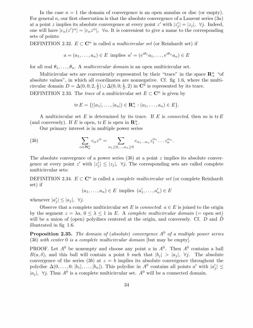
absolute values”, in which all coordinates are nonnegative. Cf. fig 1.6, where the multi-circular domain D = ∆(0, 0; 2, 1

2) ∪∆(0, 0; 12 , 2) in C2 is represented by its trace.

DEFINITION 2.33. The trace of a multicircular set E ⊂ Cn is given by

trE = (|a1|, . . . , |an|) ∈ Rn+ : (a1, . . . , an) ∈ E.

A multicircular set E is determined by its trace. If E is connected, then so is trE(and conversely). If E is open, trE is open in Rn

+.Our primary interest is in multiple power series

(3b)∑

α∈Nn0

cαzα =

∑

α1≥0,...,αn≥0

cα1...αnzα1

1 . . . zαnn .

The absolute convergence of a power series (3b) at a point z implies its absolute conver-gence at every point z′ with |z′j | ≤ |zj |, ∀j. The corresponding sets are called completemulticircular sets:

DEFINITION 2.34. E ⊂ Cn is called a complete multicircular set (or complete Reinhardtset) if

(a1, . . . , an) ∈ E implies (a′1, . . . , a′n) ∈ E

whenever |a′j| ≤ |aj |, ∀j.Observe that a complete multicircular set E is connected: a ∈ E is joined to the origin

by the segment z = λa, 0 ≤ λ ≤ 1 in E. A complete multicircular domain (= open set)will be a union of (open) polydiscs centered at the origin, and conversely. Cf. D and Dillustrated in fig 1.6.

Proposition 2.35. The domain of (absolute) convergence A0 of a multiple power series(3b) with center 0 is a complete multicircular domain [but may be empty].

PROOF. Let A0 be nonempty and choose any point a in A0. Then A0 contains a ballB(a, δ), and this ball will contain a point b such that |bj| > |aj |, ∀j. The absoluteconvergence of the series (3b) at z = b implies its absolute convergence throughout thepolydisc ∆(0, . . . , 0; |b1|, . . . , |bn|). This polydisc in A0 contains all points a′ with |a′j| ≤|aj|, ∀j. Thus A0 is a complete multicircular set. A0 will be a connected domain.

34

2.4 Convergence domains of power series and analytic continuation. Let Bdenote the set of those points z ∈ Cn at which the terms cαz

α, α ∈ Nn0 of the power

series (3b) form a bounded sequence:

(4) B = z ∈ Cn : |cαzα| ≤M = M(z) < +∞, ∀α ∈ Nn0.

The set B is clearly multicircular and it also has a certain convexity property:

Lemma 2.41. The trace of B is logarithmically convex.

PROOF. Let r′ ≥ 0 and r′′ ≥ 0 be any two points in trB. Then there is a constant M[for example, M = maxM(r′),M(r′′)] such that

|cα|(r′1)α1 . . . (r′n)αn ≤M, |cα|(r′′1 )α1 . . . (r′′n)αn ≤M, ∀α ∈ Nn0 .

It follows that for any r = (r1, . . . , rn) with components of the form rj = (r′j)1−λ(r′′j )λ

[with λ ∈ [0, 1] independent of j] and for all α’s,

|cα|rα1

1 . . . rαnn = |cα|(r′1)α1 . . . (r′n)αn1−λ|cα|(r′′1 )α1 . . . (r′′n)αnλ ≤M.

Thus r ∈ B and hence trB is logarithmically convex [Definition 2.23].

Abusing the language, a multicircular domain is called logarithmically convex whenits trace is. We can now prove

Theorem 2.42. The domain of (absolute) convergene A0 of a multiple power series (3b)with center 0 is a logarithmically convex complete multicircular domain [but may be empty].The power series will converge uniformly on every compact subset of A0.

PROOF. Consider a power series (3b) for which A0 is nonempty. We know that A0 is acomplete multicircular domain [Proposition 2.35], hence it suffices to verify its logarithmicconvexity. Clearly, A ⊂ B, cf. (4), hence A0 ⊂ B0. We will show that also B0 ⊂ A0.Choose b ∈ B0. Then B must contain a point c with |cj| = rj > |bj|, ∀j. The boundednessof the sequence of terms cαzα at z = c or z = r implies the absolute convergence ofthe power series (3b) throughout the polydisc ∆(0, r) [Lemma 1.41]. Hence b ∈ A0 sothat B0 ⊂ A0; as a result, A0 = B0. Since trB is logarithmically convex [Lemma 2.41],trA0 = trB0 will also be logarithmically convex [basically because the interior of a convexset is convex].

We know that A0 is a union of polydiscs ∆(0, s). The convergence of our power seriesis uniform on every smaller polydisc ∆(0, λs) with λ ∈ (0, 1) [Lemma 1.41], hence it isuniform on every compact subset of A0. Indeed, such a set may be covered by finitelymany polydiscs ∆(0, s) in A0 and hence by finitely many polydiscs ∆(0, λs).

COROLLARY 2.43 (Analytic continuation by power series). Suppose f is holomorphicon a complete multicircular domain D in Cn. Then f has an analytic continuation to thelogarithmically convex hull D of D. The continuation is furnished by the sum of the powerseries for f with center 0.

Indeed, D is a union of polydiscs ∆(0, r). On each of those polydiscs, the power series∑

cαzα for f with center 0 converges absolutely, and it converges to f(z), cf. Corollary

35

1.63. The domain of convergence A0 of the power series thus contains D. Being loga-rithmically convex, A0 must contain D, the smallest logarithmically convex multicirculardomain containing D. The power series is uniformly convergent on every compact subsetof D ⊂ A0. Its sum is therefore holomorphic on D; it extends f analytically throughoutD.

Fig 1.6 illustrates the case

D = ∆(0, 0; 2, 12 ) ∪∆(0, 0; 1

2 , 2)

in C2, cf. Example 2.24. Here the logarithmically convex hull D is the exact domain ofconvergence of the power series with center 0 for the function

f(z) =1

2− z1+

1

2− z2+

1

1− z1z2.

The logarithmically convex hull D of a complete multicircular domain D in Cn is atthe same time its envelope of holomorphy [Definition 2.13]. Indeed, D will be a domain ofholomorphy and (hence) also the maximal domain of existence for a certain holomorphicfunction [see Sections 6.3, 6.4.] The latter property implies that every logarithmicallyconvex complete multicircular domain is the exact domain of convergence for some powerseries with center 0.

2.5 Analytic continuation by Cauchy integrals. We will show how the Cauchyintegral or cauchy transform

(5a) fr(z)def=

1

(2πi)n

∫

T (0,r)

f(ζ)

(ζ1 − z1) . . . (ζn − zn)dζ1 . . . dζn, ∀z ∈ ∆(0, r),

can be used for analytic continuation. Here T (0, r) = C(0, r1)×. . .×C(0, rn), with positiveorientation of the circles C(0, rj).

Theorem 2.51. Let D ⊂ Cn be a connected multicircular domain containing the originand let f be holomorphic on D. Then the Cauchy transforms fr, where r > 0 runs overthe interior of traceD jointly furnish an analytic continuation of f to D′, the smallestcomplete multicircular domain containing D.

(r1,r2)

(s1,s2)

(δ1,δ2)x

x

x

R

|z2|

|z1|

tr D

ρ

tr D^

fig 2.5

36

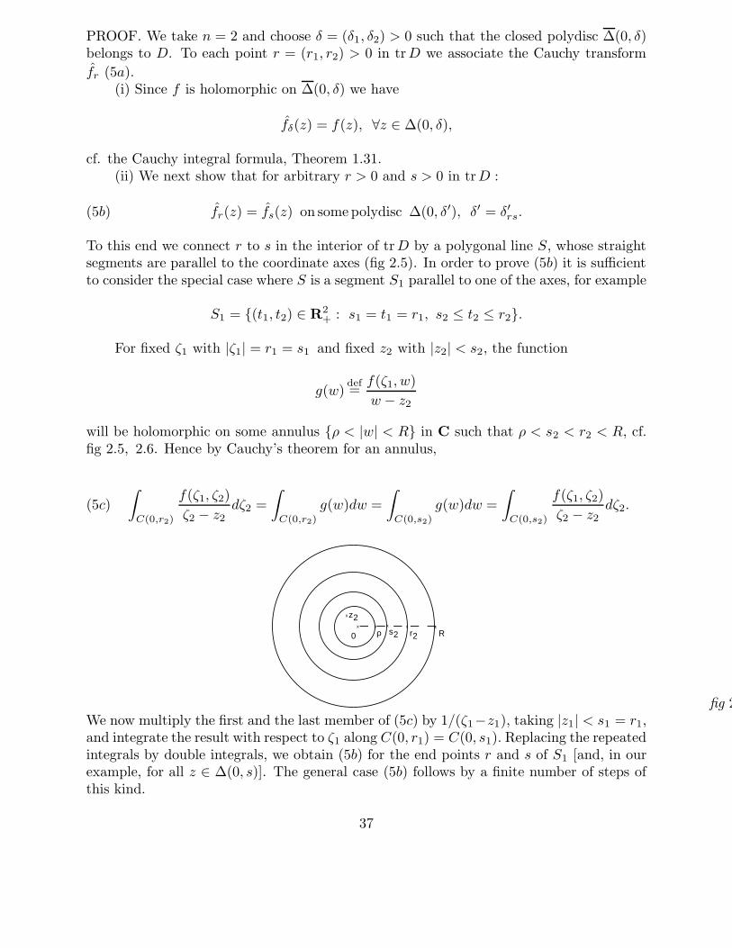
PROOF. We take n = 2 and choose δ = (δ1, δ2) > 0 such that the closed polydisc ∆(0, δ)belongs to D. To each point r = (r1, r2) > 0 in trD we associate the Cauchy transform

fr (5a).(i) Since f is holomorphic on ∆(0, δ) we have

fδ(z) = f(z), ∀z ∈ ∆(0, δ),

cf. the Cauchy integral formula, Theorem 1.31.(ii) We next show that for arbitrary r > 0 and s > 0 in trD :

(5b) fr(z) = fs(z) on some polydisc ∆(0, δ′), δ′ = δ′rs.

To this end we connect r to s in the interior of trD by a polygonal line S, whose straightsegments are parallel to the coordinate axes (fig 2.5). In order to prove (5b) it is sufficientto consider the special case where S is a segment S1 parallel to one of the axes, for example

S1 = (t1, t2) ∈ R2+ : s1 = t1 = r1, s2 ≤ t2 ≤ r2.

For fixed ζ1 with |ζ1| = r1 = s1 and fixed z2 with |z2| < s2, the function

g(w)def=f(ζ1, w)

w − z2

will be holomorphic on some annulus ρ < |w| < R in C such that ρ < s2 < r2 < R, cf.fig 2.5, 2.6. Hence by Cauchy’s theorem for an annulus,

(5c)

∫

C(0,r2)

f(ζ1, ζ2)

ζ2 − z2dζ2 =

∫

C(0,r2)

g(w)dw =

∫

C(0,s2)

g(w)dw =

∫

C(0,s2)

f(ζ1, ζ2)

ζ2 − z2dζ2.

x xx xx

0

x z2

ρ r2s2 R

fig 2.6We now multiply the first and the last member of (5c) by 1/(ζ1−z1), taking |z1| < s1 = r1,and integrate the result with respect to ζ1 along C(0, r1) = C(0, s1). Replacing the repeatedintegrals by double integrals, we obtain (5b) for the end points r and s of S1 [and, in ourexample, for all z ∈ ∆(0, s)]. The general case (5b) follows by a finite number of steps ofthis kind.

37

Combining (i) and (ii) we conclude that for every r > 0 in trD

(5d) fr(z) = f(z) on some polydisc ∆(0, δ′′), δ′′ = δ′′r .

Now the Cauchy transform fr is holomorphic on ∆(0, r) [Theorem 1.61]. It follows that

fr is equal to f throughout ∆(0, r) ∩ D [uniqueness theorem 1.54]. Jointly, the Cauchy

transforms fr furnish an analytic continuation F of f to the domain

(5e) D′ = ∪r ∆(0, r), union over all r > 0 in tr D.

D′ is the smallest complete multicircular domain containing D, cf. fig 2.5.

COROLLARY 2.52 (Once again, analytic continuation by power series). Suppose f isholomorphic on a connected multicircular domain D ⊂ Cn that contains the origin. Thenthe power series for f with center 0 converges to f throughout D and it furnishes ananalytic continuation of f to the logarithmically convex hull D of D.

Indeed, for any r > 0 in trD, the power series for fr with center 0 converges tofr on ∆(0, r) [Corollary 1.63], but this series is none other than the power series for fwith center 0, cf. (5d). Hence the latter converges to the analytic continuation F of fthroughout D′ (5e), and in particular to f throughout D. By Corollary 2.43 applied to Fand the complete multicircular domain D′, the power series for F or f around 0 actuallyprovides an analytic continuation of F or f to the logarithmically convex hull (D′)∧ of D′.

Observe finally that (D′)∧ = D. Indeed, D must containD′ [and hence (D′)∧], becauseD will contain every polydisc ∆(0, s) with s > 0 in trD, cf. Example 2.25.

2.6 Laurent series in one variable with variable coefficients; removability ofisolated singularities. Let A = A(0; ρ,R) denote the annulus 0 ≤ ρ < |w| < R ≤ +∞in C (cf. fig 2.6) and let g(w) be holomorphic on A. Then there is a unique Laurent serieswith center 0 that converges to g for some total ordering of its terms at each point of A.It is the series

(6a)

∞∑

−∞

ckwk with ck =

1

2πi

∫

C(0,r)

g(w)w−k−1dw,

where one may integrate over any (positively oriented) circle C(0, r) with ρ < r < R. Theseries actually converges absolutely, and uniformly on every compact subset of A(0; ρ,R).To prove the existence of the series representation one uses the Cauchy integral formulafor an annulus: for ρ < r1 < |w| < r2 < R,

(6b) g(w) =1

2πi

∫

C(0,r2)

g(v)

v − wdv −1

2πi

∫

C(0,r1)

g(v)

v − wdv.

The first integral gives a power series∑∞

0 ckwk on the disc ∆(0, r2) [which will in fact

converge throughout the disc ∆(0, R)]. The second integral gives a power series in 1/w,

which may be written as −∑−1−∞ ckw

k and which converges for |w| > r1 [and in fact, for

38

|w| > ρ]. Combining the series one obtains (6a). As to the other assertions above, cf.Section 2.7.

A holomorphic function g(w) on A(0; ρ,R) will have an analytic continuation to thedisc ∆(0, R) if and only if all Laurent coefficients ck with negative index are equal to 0.Indeed, if there is such a continuation [which we also call g], then by Cauchy’s theorem,the second integral in (6b) is identically zero for |w| > r1.

We now move on to Cn with n ≥ 2. Treating our complex variables z1, . . . , zn asym-metrically for the time being, we will write z′ for (z1, . . . , zn−1) and w for zn. UsingLaurent series in w with coefficients depending on z′, we will prove:

Theorem 2.61 (hartogs’ continuity theorem). Let f(z′, w) = f(z1, . . . , zn−1, w) beholomorphic on a domain D ⊂ Cn (n ≥ 2) of the form

D = D′ × A(0; ρ,R)∪D′0 ×∆(0, R),

where D′ is a connected domain in Cn−1 and D′0 a nonempty subdomain of D′ (fig 2.7).

Then f has an analytic continuation to the domain

D = D′ ×∆(0, R).

z'

ρ

R

r

x

x

x

D~

w

D'

0

D

D'

0

fig 2.7PROOF. For fixed z′ ∈ D′ the function g(w) = f(z′, w) is holomorphic in w on the annulusA(0; ρ,R), hence it may be represented by a Laurent series in w,

(6c) f(z′, w) = g(w) =∑∞

−∞ck(z′)wk.

By (6a) the coefficients are given by

(6d) ck(z′) =1

2πi

∫

C(0,r)

f(z′, w)w−k−1dw =1

2π

∫ π

−π

f(z′, reit)r−ke−iktdt, ρ < r < R.

We may now apply the holomorphy theorem for integrals [Corollary 1.72] to con-clude that each of the coefficients ck(z′) is holomorphic in z′ on D′. Indeed, f(z′, w) isholomorphic and hence continuous in (z′, w) on D. It follows that the final integrand

K(z′, t) = f(z′, reit)r−ke−ikt

39

is continuous on D′ × [−π, π]. Furthermore, for fixed t this integrand will be holomorphicin z′ on D′, because f(z′, w) is holomorphic in z′ for fixed w = reit in A(0; ρ,R).

We next observe that for fixed z′ in D′0, the function g(w) = f(z′, w) is holomorphic

on the whole disc ∆(0, R). Hence for such z′, the Laurent series (6c) must reduce to apower series. In other words, for every k < 0,

ck(z′) = 0 throughout D′0.

Thus by the uniqueness theorem for holomorphic functions, ck(z′) = 0 on all of D′ for eachk < 0. Conclusion:

(6e) f(z′, w) =∞∑

0

ck(z′)wk throughout D′ × A.

This power series with holomorphic coefficients actually defines a holomorphic functionf(z′, w) throughout D = D′ ×∆(0, R). Indeed, we will show that the series is absolutelyand uniformly convergent on every compact subset of D; Weierstrass’s theorem 1.71 onthe holomorphy of uniform limits will do the rest. Let E ′ be any compact subset of D′

and set E = E′×∆(0, s) where s < R. Choosing r ∈ (ρ,R) such that r > s, the coefficientformula (6d) furnishes a uniform estimate

|ck(z′)| ≤Mr−k for z′ ∈ E′, with M = sup|f | on E′ × C(0, r) ⊂ D.

This estimate implies the uniform convergence of the series in (6e) on E, where |w| ≤ s < r.The holomorphic sum function f on D is equal to f on D′×A and hence on D. Thus

it provides the desired analytic continuation of f to D.

APPLICATION 2.62 (Removability of isolated singularities when n ≥ 2). Let f be holo-morphic on a “punctured polydisc” D = ∆n(a, r)−a. Then f has an analytic extensionto D = ∆n(a, r).

[By translation, it may be assumed that a = 0. Now apply Theorem 2.61, taking D′ =∆n−1(0, r′) with r′ = (r1, . . . , rn−1), ρ = 0, R = rn and D′

0 = D′ − 0. An alternativeproof may be based on the one-dimensional Cauchy integral formula, cf. exercise 2.14.]

APPLICATION 2.63. Holomorphic functions on open sets Ω ⊂ Cn, n ≥ 2 can not haveisolated zeros.

[An isolated zero of f would be a nonremovable isolated singularity for 1/f.]

2.7 Multiple Laurent series on general multicircular domains. For the time being,we assume that our connected multicircular domain D in Cn does not contain any pointz with a vanishing coordinate; the exceptional case will be considered in Section 2.8.When n = 1, D is an annulus A(0; ρ,R) on which holomorphic functions are uniquelyrepresentable by Laurent series with center 0. The analog for general n is a Laurent seriesin n variables:

THEOREM 2.71. Let f be holomorphic on a connected multicircular domain D ⊂ Cn,n ≥ 1 that does not meet any hyperplane zj = 0. Then there is a unique n-variable

40

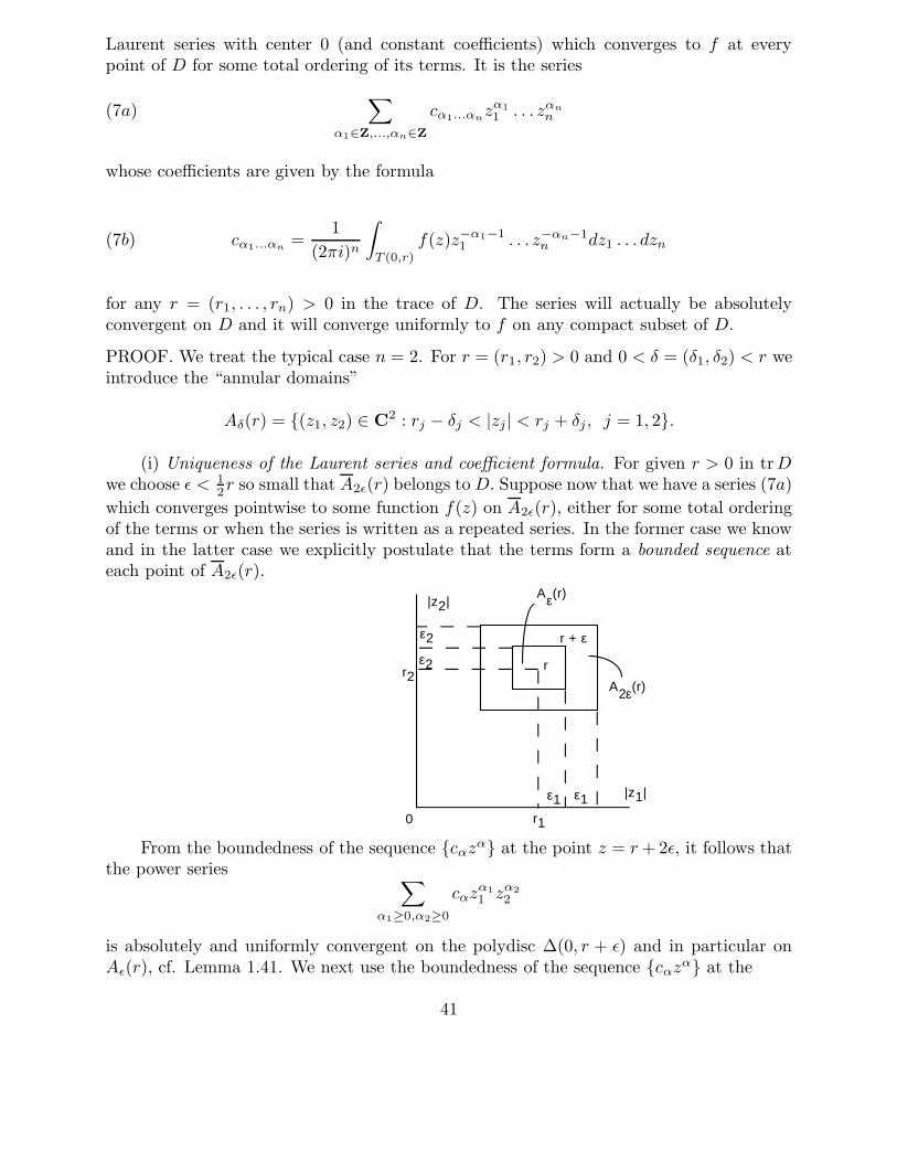
Laurent series with center 0 (and constant coefficients) which converges to f at everypoint of D for some total ordering of its terms. It is the series

(7a)∑

α1∈Z,...,αn∈Z

cα1...αnzα1

1 . . . zαnn

whose coefficients are given by the formula

(7b) cα1...αn=

1

(2πi)n

∫

T (0,r)

f(z)z−α1−11 . . . z−αn−1

n dz1 . . . dzn

for any r = (r1, . . . , rn) > 0 in the trace of D. The series will actually be absolutelyconvergent on D and it will converge uniformly to f on any compact subset of D.

PROOF. We treat the typical case n = 2. For r = (r1, r2) > 0 and 0 < δ = (δ1, δ2) < r weintroduce the “annular domains”

Aδ(r) = (z1, z2) ∈ C2 : rj − δj < |zj | < rj + δj , j = 1, 2.

(i) Uniqueness of the Laurent series and coefficient formula. For given r > 0 in trDwe choose ε < 1

2r so small that A2ε(r) belongs to D. Suppose now that we have a series (7a)

which converges pointwise to some function f(z) on A2ε(r), either for some total orderingof the terms or when the series is written as a repeated series. In the former case we knowand in the latter case we explicitly postulate that the terms form a bounded sequence ateach point of A2ε(r).

|z2|

|z1|

0 r1

r2ε2

ε1 ε1

ε2

r

A2ε(r)

Aε(r)

r + ε

fig 2.8From the boundedness of the sequence cαzα at the point z = r+ 2ε, it follows that

the power series∑

α1≥0,α2≥0

cαzα1

1 zα2

2

is absolutely and uniformly convergent on the polydisc ∆(0, r + ε) and in particular onAε(r), cf. Lemma 1.41. We next use the boundedness of the sequence cαzα at the

41

point z = (r1 − 2ε1, r2 + 2ε2) or 1/z1 = 1/(r1 − 2ε1), z2 = r2 + 2ε2. It implies that thepower series

∑

−α1>0,α2≥0

cα

(

1

z1

)−α1

zα2

2

in 1/z1 and z2 is absolutely and uniformly convergent for |1/z1| < 1/(r1−ε1) or |z1| > r1−ε1and |z2| < r2+ε2, hence in particular on Aε(r). Also using the boundedness of the sequencecαzα at z = r − 2ε and at z = (r1 + 2ε1, r2 − 2ε2), we conclude that the whole series(7a) is absolutely and uniformly convergent on Aε(r). The sum will be equal to f(z) forany arrangement of the terms.

Termwise integration of the absolutely and uniformly convergent series

f(z)z−β−1 =∑

α∈Z2

cαzα−β−1 [β + 1 = (β1 + 1, β2 + 1)]

over the torus T (0, r) in Aε(r) gives

(7c)1

(2πi)2

∫

T (0,r)

f(z)z−β−1dz =∑

α

cα1

(2πi)2

∫

T (0,r)

zα−β−1dz,

where dz stands for dz1dz2. Since

1

2πi

∫

C(0,rj)

zαj−βj−1j dzj =

1 for αj = βj

0 for αj 6= βj ,

the sum in (7c) reduces to cβ . We have thus proved formula (7b) at least for n = 2 andwith β instead of α.

If f is represented by a series (7a) at each point of D [in the sense indicated at thebeginning of (i)], the coefficients are given by (7b) for each r > 0 in trD, hence such arepresentation is surely unique. We will then have absolute and uniform convergence of theLaurent series on any compact subset E ⊂ D, since such an E can be covered by finitelymany annular domains Aε(r) for which A2ε(r) belongs to D.

(ii) Existence of the Laurent series. Let f be holomorphic on D. For r > 0 in trD, sothat T (0, r) ⊂ D, the right-hand side of (7b) defines coefficients cα(r) which might dependon r. Do they really? No, using the method of polygonal lines as in part (ii) of the proofof Theorem 2.51, one readily shows that cα(r) is independent of r. Indeed, referring tofig 2.5,

∫

C(0,r2)

f(z1, z2)z−α2−12 dz2 =

∫

C(0,s2)

f(z1, z2)z−α2−12 dz2

whenever z1 ∈ C(0, r1) = C(0, s1). Multiplying by z−α1−11 and integrating with respect to

z1, one concludes that cα(r) = cα(s).Thus we may use (7b) to associate constant coefficients cα to f . With these coefficients,

the terms in the series (7a) will form a bounded sequence at each point of D. Indeed, choosew in D and take rj = |wj |, j = 1, 2 [as we may]. Then by (7b),

42

(7d)

|cα1α2wα1

1 wα2

2 | =∣

∣

∣

∣

∣

1

(2πi)2

∫

T (0,r)

f(z)

(

w1

z1

)α1(

w2

z2

)α2 dz1z1

dz2z2

∣

∣

∣

∣

∣

≤ sup T (0,r) |f(z)|, ∀α.

We now fix r > 0 in trD and take ε < r so small that Aε(r) belongs to D. For fixedz2 in the annulus r2 − ε2 < |z2| < r2 + ε2, the function f(z1, z2) is holomorphic in z1 onthe annulus r1 − ε1 < |z1| < r1 + ε1, hence f has the absolutely convergent one-variableLaurent representation

(7e) f(z1, z2) =∑

α1∈Z

dα1(z2)zα1

1 , z ∈ Aε(r)

with

(7f)

dα1(z2) =

1

2πi

∫

C(0,r1)

f(z1, z2)z−α1−11 dz1

=1

2π

∫ π

−π

f(r1eit, z2)r−α1

1 e−iα1tdt .

The coefficients dα1(z2) will be holomorphic on the annulus r2 − ε2 < |z2| < r2 + ε2,

cf. the holomorphy theorem for integrals 1.72. Hence the coefficients have the absolutelyconvergent Laurent representations

(7g) dα1(z2) =

∑

α2∈Z

dα1α2zα2

2

with

(7h) dα1α2= dα1α2

(r) =1

2πi

∫

C(0,r2)

dα1(z2)z−α2−1

2 dz2.

Substituting (7g) into (7e) we finally obtain the representation

f(z1, z2) =∑

α1

∑

α2

dα1α2(r)zα2

2

zα1

1 , ∀z ∈ Aε(r).

Here by (7h) and (7f), also making use of the continuity of f on T (0, r) to rewrite arepeated integral as a double integral,

43

dα1α2(r) =

1

(2πi)2

∫

C(0,r2)

∫

C(0,r1)

f(z1, z2)z−α1−11 dz1

z−α2−12 dz2

=1

(2πi)2

∫

T (0,r)

f(z1, z2)z−α1−11 z−α2−1

2 dz1dz2 = cα1α2(r) = cα1α2

.

Conclusion: f has a representation as a series (7a, b), locally on D and hence globally,when the terms are arranged in a repeated series. The terms form a bounded sequenceat each point w ∈ D (7d). Thus by part (i), the corresponding double series is absolutelyconvergent and hence converges to f on D for any arrangement of the terms.

2.8 Spherical shell theorem. In C, a connected multicircular domain D containing thepoint w = 0 is just a disc around 0. In that case the Laurent series (6a) for f ∈ O(D) onD−0 reduces to a power series: ck = 0 for all k < 0. Something similar happens in Cn:

LEMMA 2.81. Let D ⊂ Cn be a connected multicircular domain containing a point b withjth coordinate bj = 0. Let f be holomorphic on D and let

∑

cαzα be its Laurent series

(7a, b) on D = D − z ∈ Cn : z1 . . . zn = 0. [All points with a vanishing coordinate havehere been removed from D so as to make Theorem 2.71 applicable as it stands.] Thencα1...αn

= 0 for all α’s with αj < 0.|z2|

|z1|

0 r1

(0,r2)

tr D

(r1,r2)

fig 2.9

PROOF. We may take n = 2 and j = 1. Shifting b = (0, b2) a little if necessary, wemay assume r2 = |b2| 6= 0 [D is open]. Since trD is open in R2

+, it will contain ashort closed horizontal segment from the point (0, r2) to a point (r1, r2) > 0. D willthen contain all points (z1, z2) with |z1| ≤ r1, |z2| = r2 (fig 2.9). Thus for each fixedz2 ∈ C(0, r2), f(z1, z2) will be analytic in z1 on the closed disc |z1| ≤ r1. Hence byCauchy’s theorem,

∫

C(0,r1)

f(z1, z2)z−α1−11 dz1 = 0 for z2 ∈ C(0, r2)

whenever −α1 − 1 ≥ 0. Conclusion:

44

cα1α2=

1

(2πi)2

∫

C(0,r2)

(∫

C(0,r1)

f(z1, z2)z−α1−11 dz1

)

z−α2−12 dz2 = 0, ∀α1 < 0.

We single out the important case where D meets each of the hyperplanes zj = 0 :

THEOREM 2.82 (Analytic continuation based on multiple Laurent series). Let D ⊂ Cn

be a connected multicircular domain which for each j, 1 ≤ j ≤ n contains a point z withzj = 0, and let f be any holomorphic function on D. Then the Laurent series for f on

D = D − z1 . . . zn = 0 with center 0 is a power series. Its sum function furnishes ananalytic continuation of f to the logarithmically convex hull D of D.

PROOF. By Lemma 2.81 the Laurent series (7a, b) for f [on D] has cα = cα1...αn= 0

whenever [at least] one of the numbers αj is negative, hence the Laurent series is a power

series. This power series converges to f throughout D [Theorem 2.71], hence it convergeson every polydisc ∆(0, r) with r > 0 in tr D or trD [Proposition 1.42]. Since the sum isequal to f on ∆(0, r) ∩ D it is equal to f on ∆(0, r) ∩D [uniqueness theorem] and hencethroughout D. Naturally, the power series furnishes an analytic continuation of f to thesmallest complete multicircular domain D′ containing D and to its logarithmically convexhull (D′)∧, cf. the discussion following Corollary 2.52. As in that case, (D′)∧ will coincidewith D. [Indeed, D will contain a neighbourhood of the origin, cf. exercise 2.7, hence itcontains every polydisc ∆(0, s) with s > 0 in trD (fig 2.4), and thus D contains D′.]

Application 2.83 (hartogs’ spherical shell theorem). Let f be holomorphic onthe spherical shell given by ρ < |z| < R in Cn with n ≥ 2, ρ ≥ 0. Then f has an analyticcontinuation to the ball B(0, R).

[A more general theorem of this kind will be proved in Chapter 3.]

2.9 Envelopes of holomorphy may extend outside Cn ! We will first construct adomain D in C2 and a Riemann domain X over C2 with the following property: everyholomorphic function on D can be continued analytically to X, and the Riemann domainX is really necessary to accomodate single-valued analytic continuations of all functionsin O(D).

We start with the multicircular domain D0 in C2 given by

D0 = |z1| < 1, |z2| < 2 ∪ |z1| < 2, 1 < |z2| < 2.

[Make a picture of trace D0 ! Fig 2.11 shows, among other things, the 3-dimensional in-tersection of D0 with the real hyperplane y2 = 0.] As we know, every function in O(D0)extends analytically to the bidisc ∆(0, 2) = ∆(0, 0; 2, 2), cf. Section 2.5.

45

γ

4i

T

z1-plane

T1

x

0

x

fig 2.10

We next choose an arc γ of the circle C(4i, 4) in the z1-plane (z2 = 0) as follows: γstarts at the origin and, running counterclockwise, it terminates in the half-planeRe z1 < 0 between the circles C(0, 1) and C(0, 2) (fig 2.10). For example,

γ : z1 = 4i+ 4eit, z2 = 0, −π/2 ≤ t ≤ 3π/2− π/8.

Around this arc we construct a thin tube T in C2, say an ε-neighbourhood of γ. Here ε ischosen so small that the part

T1def= T ∩∆(0, 2) ∩ Re z1 < 0

does not meet D0. Our domain D ⊂ C2 will be (cf. fig 2.11)

Ddef= D0 ∪ T.

Do

(4i,0)

(y2 =0)

T

T1

x

x

fig 2.11Now let f be any function in O(D). Then the restriction f | D0 has an analytic

continuation to ∆(0, 2). However, on the part T1 of T that continuation may very well be

46

different from the original function f . For example, one may take for f(z) that holomorphicbranch of

log(z1 − 4i) on D

for which Im f runs from −π/2 to 3π/2 − π/8 on γ. On T1 the values of Im f will beapproximately 3π/2− π/8, while on the part of T close to the origin, Im f will be approx-imately −π/2. Hence the analytic continuation f ∗ of the restriction f | D0 to ∆(0, 2) willhave its imaginary part on T1 in the vicinity of π/2− π/8 !

All functions in O(D) have an analytic continuation to a Riemann domain X overC2 which contains ∆(0, 2) and a copy of the tube T . The two are connected whereRe z1 > 0, but where T (going “counterclockwise”) again reaches ∆(0, 2), now in the half-space Re z1 < 0, the end T1 must remain separate from ∆(0, 2): it may be taken “over∆(0, 2)”.

SIMULTANEOUS ANALYTIC CONTINUATION: general theory. The construction ofthe maximal Riemann continuation domain R for a holomorphic function f in Section 2.1can be extended to the case of simultaneous analytic continuation for the members of afamily of holomorphic functions. We deal with indexed families; in the following discussion,the index set Λ is kept fixed. Mimicking the procedure for a single function, we now defineΛ-elements (a, U, fλ) at points a ∈ Cn. Such elements consist of a connected domainU ⊂ Cn containing a and a family of functions fλ ⊂ O(U) with index set Λ. TwoΛ-elements (a, U, fλ) and (a, U, fλ) at the same point a are called equivalent if thepower series (fλ)a and (fλ)a agree for every λ ∈ Λ. A Λ-element (b, V, gλ) is called adirect Λ-continuation of (a, U, fλ) if V ∩ U is nonempty and gλ = fλ, ∀λ on a fixedcomponent of V ∩ U . General Λ-continuations are introduced by means of both finitechains and continuous chains of direct Λ-continuations.

Starting with a given Λ-element (a, U, fλ) and carrying out unlimited Λ-continua-tion, one arrives at a Riemann domain X = (X, π) over Cn whose points p are equivalenceclasses of Λ-continuations at points b ∈ Cn: let us write p = [(b, V, gλ)]. Basic neigh-bourhoods N = N (p, V, gλ) in X shall consist of the points q corresponding to the directΛ-continuations (c,W, hλ) of (b, V, gλ) for which c ∈ V and (hλ)c = (gλ)c, ∀λ. Theprojection π : π(p) = b, when restricted to N , establishes a homeomorphism of N in Xonto V in Cn. Every function fλ of the original Λ-element has an analytic continuationFλ to X given by Fλ(p) = gλ(b). Indeed,

Fλ(q) = hλ(z) = gλ(z), ∀q = [(z,W, hλ)] ∈ N (p, V, gλ),

so that Fλ is holomorphic on X in the accepted sense: on N ⊂ X it is given by an ordinaryholomorphic function on the domain V = π(N ) ⊂ Cn. Finally, setting p0 = [(a, U, fλ)]and identifying N (p0, U, fλ) with U , one has Fλ = fλ on U .

We have thus obtained a common continuation domainX for the family of holomorphicfunctions fλ on U . It is plausible and one can show that this “Λ-continuation domain”X is maximal; one speaks of a Λ-envelope for U , cf. [Narasimhan].

47

APPLICATION 2.91 (Envelope of holomorphy). Let D be a connected domain in Cn.Applying the preceding construction to U = D or U ⊂ D and Λ = O(D), one obtains anO(D)-continuation domain XD = (XD, π) for D. Being maximal, XD is called an envelopeof holomorphy for D. Every function f ∈ O(D) has a (unique) analytic continuationFf to XD. On a suitable neighbourhood N of p in XD, the functions Ff are given byFf (q) = gf (z), z = π q, where the functions gf on V = π(N ) may be obtained from thefunctions f on U by analytic continuation along a common path. Observe in particularthat for f ≡ c, also Ff ≡ c. More generally, if Ff = c on some neighbourhood N in X,then Ff = c everywhere.

What was said in the last four sentences is also true for arbitrary (connected) O(D)-continuation domains X for D, in or over Cn. It is perhaps surprising that on such adomain X, the analytic continuations f ∗ of the functions f ∈ O(D) can not take on newvalues:

PROPOSITION 2.92. Suppose that the equation f(z) = c, c ∈ C has no solution z ∈ D.Then the equation f∗(q) = c can not have a solution q in any O(D)-continuation domainX.

Indeed, by the hypothesis there is a function g ∈ O(D) such that

f(z)− cg(z) ≡ 1 on D.

Introducing the simultaneous analytic continuations to X, one obtains

f∗(q)− c g∗(q) = (f − c)∗(q) g∗(q) = 1∗ = 1 on X.

It is not hard to deduce the following corollary, cf. exercise 2.24:

COROLLARY 2.93. Let D ⊂ D′ be a connected domain in Cn to which all functions inO(D) can be continued analytically. Then D′ belongs to the convex hull CH(D).

Exercises

2.1. Give an example of two function elements (a, U, f), (b, V, g) such that g = f on onecomponent of V ∩ U , while g 6= f on another component.

2.2. Let b be an arbitrary boundary point of the polydisc ∆(0, r) in C2. Show that there isa holomorphic function on ∆(0, r) that tends to infinity as z → b. [One may concludethat ∆(0, r) is a domain of holomorphy, cf. Section 1.9.]

2.3. Prove that hulls of holomorphy in Cn are unique when they exist [Definition 2.13].

2.4. (i) Let E be a compact convex set in Rn and let V be a supporting hyperplane.Prove that the intersection E ∩ V is also a compact convex set.

(ii) Let S be a compact subset of Rn. Prove the Caratheodory representation (2) forthe points of the convex hull CH(S) with m ≤ n+ 1.

2.5. Let S be a compact set in Rn. Show that

48

(i) For every direction (or unit vector) c there is a point b ∈ S such thatmaxx∈S c · x = c · b ;

(ii) The convex hull CH(S) is the set of all points x ∈ Rn such that c·x ≤ max s∈S c·sfor every vector c ∈ Rn.

2.6. What sort of equation “y = f(x)” does the logarithmically convex hull of the set oftwo points r′ > 0 and r′′ > 0 in R2

+ = (r1, r2) ≥ 0 have?

2.7. Determine the logarithmically convex hull in R2+ of :

(i) the set s, t of two points s = (s1, s2) > 0 and t = (t1, 0);(ii) the set s, t when s = (s1, 0) and t = (0, t2);

(iii) the set consisting of the neighbourhood s1 − ε < r1 < s1 + ε, 0 ≤ r2 < ε of(s1, 0) and the neighbourhood 0 ≤ r1 < ε, t2 − ε < r2 < t2 + ε of (0, t2).

2.8. Prove that a closed or open set F in Rn+ is logarithmically convex if and only if r′ ∈ F

and r′′ ∈ F always implies that r = (r′r′′)12 is in F . Deduce that the unit ball

B = B(0, 1) in C2 is logarithmically convex [that is, trB is logarithmically convex].

2.9. Let S = S(0, 1) denote the unit sphere in Cn ∼ R2n :

S = z ∈ Cn : z1z1 + . . .+ znzn = 1

and let b be any point of S. Show that(i) The (2n−1)-dimensional (real) tangent hyperplane to S at b may be represented

by the equation Re (b · z) = 1;(ii) Re (b · z) < 1 throughout the unit ball B;

(iii) The complex tangent hyperplane at b, of complex dimension n−1 (real dimension2n− 2) may be represented by the equation c · (z − b) = 0 with c = . . . ;

(iv) There is a holomorphic function f on the unit ball B that tends to infinity asz → b. [Thus B is a domain of holomorphy, cf. Section 1.9.]

2.10. Let D be a connected (multicircular) domain in C2. Prove that D − z1 = 0 andD − z1z2 = 0 are also connected (multicircular) domains.

2.11. Prove that the multicircular domain in C2 given by |z1| < 2, |z2| < 2, |z1z2| < 1 isa domain of holomorphy. [Cf. exercise 2.2.]

2.12. (Relation between the sets A and A0 of Section 2.3) Let∑

cαzα be a multiple power

series with center 0. Prove that every point a ∈ A (point of absolute convergence)with |aj | > 0, ∀j belongs to closA0. Then give an example to show that a point b ∈ Afor which one coordinate is zero may be very far from A0.

2.13. Let∑

cαzα be a power series in C2 for which ∆(0, 0; r1, r2) is a polydisc of convergence

that is maximal for the given r1 as far as r2 is concerned, that is, the power seriesdoes not converge throughout any polydisc ∆(0, 0; r1, s2) with s2 > r2. Prove that thesum function f(z) of the power series must become singular somewhere on the torusT (0, r) = C(0, r1) × C(0, r2). [Hence if f ∈ O(∆(0, r)) becomes singular at a pointb in ∆1(0, r1)× C(0, r2), it must have a singularity on every torus C(0, ρ)× C(0, r2)with |b1| < ρ ≤ r1.]

49

2.14. (Analytic continuation across a compact subset) Let D ⊂ C2 be the domain given by

|z1| < 1 + ε, 1− ε < |z2| < 1 + ε ∪ 1− ε < |z1| < 1 + ε, |z2| < 1 + ε, (0 < ε < 1),

or more generally, let D be any connected domain in Cn (n ≥ 2) that contains theboundary ∂∆(0, 1) of the unit polydisc, but not all of ∆(0, 1) itself. Let f be anyfunction in O(D). Prove that the formula

F (z)def=

1

2πi

∫

C(0,1)

f(z′, w)

w − zndw, z ∈ ∆(0, 1), z′ = (z1, . . . , zn−1)

furnishes an analytic continuation of f to ∆(0, 1).

2.15. Let B denote the set of those points z ∈ Cn at which the terms cαzα, α ∈ Zn of

the Laurent series (3a) form a bounded sequence. Prove that (the trace of) B islogarithmically convex.

2.16. Prove that the domain of (absolute) convergence A0 of a Laurent series with center 0in Cn is logarithmically convex.

2.17. Let D be a multicircular domain in Cn which contains the origin, or which at leastfor each j contains a point z with zj = 0. Prove that the logarithmically convex hull

D contains the whole polydisc ∆(0, s) whenever s > 0 belongs to trD.

2.18. Use appropriate results to determine the envelopes of holomorphy for the followingmulticircular domains in C2 :

(i) |z1| < 1, |z2| < 2 ∪ |z1| < 2, 1 < |z2| < 2;(ii) 1 < |z1| < 2, |z2| < 2 ∪ |z1| < 2, 1 < |z2| < 2.

2.19. Let f be holomorphic on Cn, n ≥ 2 and f(0) = 0. Prove that the zero set Zf of f isclosed but unbounded.

2.20. Let f be holomorphic on D = B(0, 1)− z1 = 0 in C2. Suppose f has an analyticcontinuation to a neighbourhood of the point (0, 1

2). Prove that f has an analytic

continuation to B(0, 1).

2.21. Let D be a multicircular domain in C2 that contains the point (0, r2) with r2 > 0 andlet ε = (ε1, ε2) > 0 be so small that D contains the closure of the domain U2ε givenby |z1| < 2ε1, r2 − 2ε2 < |z2| < r2 + 2ε2. Prove that the Laurent series for f ∈ O(D)is absolutely and uniformly convergent on Uε. [Cf. Lemma 2.81 and part (i) of theproof of Theorem 2.71.]

2.22. (Isolated singularities in Cn, n ≥ 2 are removable) Give two alternative proofs forApplication 2.62.

2.23. Derive the spherical shell theorem from Hartogs’ continuity theorem. [Let f be holo-morphic for ρ < |z| < R and suppose that the boundary point (ρ, 0, . . . , 0) would besingular for f .]

50

2.24. Let D ⊂ Cn be connected and bounded and let D′ ⊂ Cn be a connected domaincontaining D to which all functions in O(D) can be continued analytically. Determinethe analytic continuations of the functions f(z) = c · z, where c = α − iβ ∈ Cn andprove that

Re c · z ≤ max ζ∈D Re c · ζ, ∀z ∈ D′.

Deduce that D′ belongs to the convex hull of D, hence of D. [Cf. exercise 2.5.]

2.25. Let D ⊂ C2 be a bounded connected multicircular domain containing the origin. Usethe monomials p(z) = zα1

1 zα2

2 to show that a point z ∈ C2 outside the closure of the

logarithmically convex hull D of D can not belong to an O(D)-continuation domainD′ ⊃ D in C2.

2.26. Try to find an example of a domain D in Cn, for which the envelope of holomorphyXD over Cn has infinitely many layers.

51

CHAPTER 3

Analytic continuation, part II

This chapter deals with more recent methods of analytic continuation, based on the∂ equation and the so-called partial derivatives lemma.

We have already discussed Hartogs’ spherical shell theorem 2.83, but there is a muchmore general result on the removal of compact singularity sets, the Hartogs-Osgood-Browncontinuation theorem [Section 3.4]. We will present a modern proof of that result (due toEhrenpreis) in which one starts with a C∞ continuation g across an appropriate compactset and then subtracts off the “nonanalytic part” u, cf. Section 1.9. In the present instancethe correction term u has to satisfy a ∂ equation

∂u = v =

n∑

1

vjdzj or∂u

∂zj= vj , j = 1, . . . , n

on Cn with C∞ coefficients vj of compact support. The analytic continuation problemrequires a smooth solution u on Cn which likewise has compact support. The local inte-grability conditions

∂vk/∂zj = ∂vj/∂zk, ∀ j, k

being satisfied, it turns out that there is a compactly supported solution u whenever n ≥ 2[Section 3.2]. It will be obtained with the aid of a useful one-variable device, Pompeiu’sintegral formula for smooth functions.

There are various situations in real and complex analysis where one has good boundson a family of directional derivatives

(

d

dt

)m

f(a+ tξ)∣

∣

t=0, ξ ∈ E ⊂ S(0, 1), m = 1, 2, . . . (a fixed)

of a C∞ function f . If the set of directions E is substantial enough, a partial derivativeslemma of the author and Wiegerinck provides related bounds for all derivatives Dαf(a).Under appropriate conditions, the power series for f with center a can then be used foranalytic extension.

To illustrate the method we give a simple proof of the Behnke–Kneser “recessed-edgetheorem” [Section 3.5]. Another application leads to a form of Bogolyubov’s famous edge-of-the-wedge theorem. This result which came from a problem in quantum field theoryprovides a remarkable Cn extension of Schwarz’s classical reflection principle.

3.1 Inhomogeneous Cauchy-Riemann equation for n = 1. As preparation for thecase of Cn we consider the case of one variable,

(1a)∂u

∂z=

1

2

(

∂u

∂x− 1

i

∂u

∂y

)

= v on C,

52

where v is a function with compact support. The support, abbreviation supp, of a function[or distribution, or differential form] is the smallest closed set outside of which it is equalto zero. Our functions v(z) = v(x + iy) will be smooth, that is, at least of class C1 onC = R2 as functions of x and y.

For the solution of equation (1a) we start with pompeiu’s formula [also called theCauchy-Green formula]:

Proposition 3.11. Let D be a bounded domain in C whose boundary Γ consists of finitelymany piecewise smooth Jordan curves, oriented in such a way that D lies to the left of Γ.Let f(z) = f(x+ iy) be of class C1 on D as a function of x and y. Then

(1b) f(a) =1

2πi

∫

Γ

f(z)

z − adz −1

π

∫

D

∂f

∂z

1

z − adxdy, ∀a ∈ D.

Observe that the area integral over D is well-defined because 1/(z − a) is absolutelyintegrable over a neighbourhood of a, cf. the proof below. Formula (1b) reduces to Cauchy’sintegral formula if f is holomorphic on D, so that ∂f/∂z = 0. The formula occurred inwork of Pompeiu around 1910, but its usefulness for complex analysis only became apparentaround 1950.

The proof will be based on green’s formula for integration by parts in the plane:

∫

∂D

Pdx+Qdy =

∫

D

(

∂Q

∂x− ∂P

∂y

)

dxdy,

where P (x, y) and Q(x, y) are functions of class C1(D) and ∂D denotes the oriented bound-ary of D. Applied to P = F and Q = iF with F (z) = F (x + iy) in C1(D), we obtain acomplex form of Green’s formula:

(1c)

∫

∂D

F (z)dz =

∫

∂D

Fdx+ iFdy =

∫

D

(

i∂F

∂x− ∂F

∂y

)

dxdy

= 2i

∫

D

∂F

∂zdxdy.

a x

Dε

εεΒ

-C(a, )ε

Γfig 3.1

PROOF of Proposition 3.11. One would like to apply Green’s formula (1c) to the function

53

F (z) =f(z)

z − a, a ∈ D.

However, this F is in general not smooth at z = a. We therefore exclude a small closeddisc Bε = B(a, ε) from D, of radius ε < d(a,Γ). Below, we will apply Green’s formula toF on

Dεdef= D − Bε.

The correctly oriented boundary ∂Dε will consist of Γ and −C(a, ε): the circle C(a, ε)traversed clockwise.

Since 1/(z−a) is holomorphic throughout Dε, the product rule of differentiation gives

∂F

∂z=∂f

∂z

1

z − a + f(z)∂

∂z

1

z − a =∂f

∂z

1

z − a , z ∈ Dε.

Thus by (1c),

(1d)

∫

Γ

f(z)

z − adz +

∫

−C(a,ε)

f(z)

z − adz = 2i

∫

Dε

∂f

∂z

1

z − adxdy.

Passage to the limit as ε ↓ 0 will give (1b). Indeed, by the continuity of f at a,

∫

−C(a,ε)

f(z)

z − adz = −i∫ π

−π

f(a+ εeit)dt→ −2πif(a) as ε ↓ 0.

Furthermore, since ∂f/∂z is continuous on D while 1/(z − a) is (absolutely) integrableover discs B(a,R), the product is integrable over D, hence the last integral in (1d) willtend to the corresponding integral over D. In fact, if M denotes a bound for |∂f/∂z| onD, then

∫

D

−∫

Dε

=

∫

Bε

∂f

∂z

1

z − adxdy

≤M∫

Bε

1

|z − a|dxdy

= M

∫ ε

0

∫ π

−π

1

rr drdt = M 2πε→ 0 as ε ↓ 0.

Corollary 3.12. Any C1 function f(z) = f(x+ iy) on C of compact support has therepresentation

(1e) f(z) = − 1

π

∫

C

∂f

∂z(ζ)

1

ζ − z dξdη (ζ = ξ + iη), ∀z ∈ C.

Indeed, fixing a ∈ C, one may apply Pompeiu’s formula (1b) to a disc D = B(0, R)which contains both a and the support of f . Then the integral over Γ = C(0, R) willvanish; the integral over D = B(0, R) will be equal to the corresponding integral over Cor over supp f . One may finally replace the variable z under the integral sign in (1b) byζ = ξ + iη and then replace a by z.

54

Formula (1e) can also be verified directly and the condition that f have compactsupport may be relaxed to a smallness condition on f and ∂f/∂z at infinity, cf. exercises3.1, 3.2. Thus if our equation ∂u/∂z = v has a solution which is small at infinity, it willbe given by the cauchy-green transform u of v :

(1f) u(z)def= − 1

π

∫

C or supp v

v(ζ)

ζ − z dξdη (ζ = ξ + iη), ∀z ∈ C.

We will show that this candidate is indeed a solution:

Theorem 3.13. Let v be a Cp function (1 ≤ p ≤ ∞) on C of compact support [briefly,v ∈ Cp0 (C)]. Then the Cauchy-Green transform u of v (1f) provides a Cp solution of theequation ∂u/∂z = v on C. It is the unique smooth solution which tends to 0 as |z| → ∞.PROOF. Replacing ζ by ζ ′ + z in (1f) and dropping the prime ′ afterwards, we may writethe formula for u as

(1g) u(z) = − 1

π

∫

C

v(z + ζ ′)

ζ ′dξ′dη′ = − 1

π

∫

C

v(z + ζ)

ζdξdη.

We will show that u has first order partial derivatives and that they may be obtained bydifferentiation under the integral sign. Fixing a and varying z = a + h over a small discB(a, r), the function v(z + ζ) will vanish for all ζ outside a fixed large disc B = B(0, R).Focusing on ∂u/∂x we take h real and 6= 0, so that

(1h)v(a+ h+ ζ)− v(a+ ζ)

h− ∂v

∂x(a+ ζ) =

1

h

∫ h

0

∂v

∂x(a+ t+ ζ)− ∂v

∂x(a+ ζ)

dt.

Since ∂v/∂x is continuous and of compact support it is uniformly continuous on C, hencethe right-hand side ρ(ζ, h) of (1h) tends to 0 as h → 0 uniformly in ζ. Multiplying (1h)by the absolutely integrable function 1/ζ on B and integrating over B, we conclude that

−πu(a+ h)− u(a)

h−∫

B

∂v

∂x(a+ ζ) · 1

ζdξdη =

∫

B

ρ(ζ, h)1

ζdξdη → 0

as h→ 0. Thus the partial derivative ∂u/∂x exists at a and

(1i)∂u

∂x(a) = − 1

π

∫

B or C

∂v

∂x(a+ ζ) · 1

ζdξdη.

The uniform continuity of ∂v/∂x also ensures continuity of ∂u/∂x.Differentiation with respect to y goes in much the same way, hence u is of class C1.

Combining the partial derivatives we find that

(1j)∂u

∂z(a) = − 1

π

∫

C

∂v

∂z(a+ ζ) · 1

ζdξdη = − 1

π

∫

C

∂v

∂z(ζ)

1

ζ − adξdη.

Now v is a Cp function of bounded support, hence by Corollary 3.12, the final member of(1j) is equal to v(a). Thus u satisfies the differential equation (1a).

55

If p ≥ 2, one may also form higher order partial derivatives by differentiation underthe integral sign in (1g) to show that all partial derivatives of u of order ≤ p exist and arecontinuous on C.

The Cauchy-Green transform u(z) tends to 0 as |z| → ∞ and it is the only smoothsolution of (1a) with that property. Indeed, the other smooth solutions have the formu+ f , where f is smooth and satisfies the Cauchy-Riemann condition ∂f/∂z = 0, hence fmust be an entire function. However, by Liouville’s theorem, f(z)→ 0 as |z| → ∞ only iff ≡ 0.

REMARKS 3.14. For v ∈ Cp0 , p ∈ N0, the Cauchy-Green transform u (1f) will actuallybe of class Cp+α, ∀α ∈ (0, 1): u ∈ Cp and its partial derivatives of order p will satisfy aLipschitz condition of order α, cf. exercise 3.6. In general, the transform u will not havecompact support, in fact, as |z| → ∞,

zu(z)→ (1/π)

∫

C

v(ζ)dξdη

and this limit need not vanish. [Cf. also exercise 3.5.] Formula (1f) defines a function uunder much weaker conditions than we have imposed in the Theorem: continuity of v andintegrability of |v(ζ)/ζ| over C will suffice. The corresponding transform u will be a weakor distributional solution of equation (1a), cf. exercise 3.8.

3.2 Inhomogeneous C −R equation for n ≥ 2, compact support case. Saying thata differential form

(2a) f =n∑

j=1

(ujdzj + vjdzj)

is defined and of class Cp on Ω ⊂ Cn means that the coefficients uj , vj are defined andof class Cp on Ω as functions of the real variables x1, y1, . . . , xn, yn. By definition, such aform vanishes on an open subset of Ω only if all coefficients vanish there. There will be amaximal open subset of Ω on which f = 0; its complement in Ω is the support of f . Thedifferential form f in (2a) is called a first order form or a 1-form; if it contains no termsujdzj , one speaks of a (0, 1)-form.

Theorem 3.21. Let E be a compact subset of Cn, n ≥ 2 with connected complementEc = Cn −E. Let

v =n∑

1

vjdzj

be a (0, 1)-form of class Cp (1 ≤ p ≤ ∞) on Cn whose support belongs to E and whichsatisfies the integrability conditions ∂vk/∂zj = ∂vj/∂zk, ∀ j, k. Then the equation ∂u = v,or equivalently, the system

(2b)∂u

∂zj= vj , j = 1, . . . , n

56

has a unique solution u of class Cp on Cn with support in E.

A result of this kind is sometimes called a Grothendieck-Dolbeault lemma, cf.[Grauert-Remmert]. The solution u will actually be of class Cp+α, ∀α ∈ (0, 1), see exercise3.9. For arbitrary compact E, supp u need not be contained in supp v [cf. the proof below].

PROOF. We will solve the first equation (2b) by means of the Cauchy-Green transformrelative to z1, cf. Theorem 3.13. It will then miraculously follow from the integrabilityconditions that the other equations are also satisfied!

It is convenient to set (z2, . . . , zn) = z′, so that z = (z1, z′). For fixed z′, the smooth

function v1(z1, z′) of z1 has bounded support in C, hence Theorem 3.13 gives us a solution

of the equation ∂u/∂z1 = v1 in the form of the Cauchy-Green transform of v1 relative toz1 :

(2c) u(z) = u(z1, z′) = − 1

π

∫

C

v1(ζ, z′)

ζ − z1dξdη = − 1

π

∫

C

v1(z1 + ζ, z′)

ζdξdη, z ∈ Cn.

Here the integration variable ζ = ξ + iη runs just over the complex plane. The methodof differentiation under the integral sign of Section 3.1, applied to the last integral, showsthat u is of class Cp on Cn as a function of x1, y1, . . . , xn, yn.

We now go back to the first integral in (2c) to obtain an expression for ∂u/∂zj whenj ≥ 2. In the second step below we will use the integrability condition ∂v1/∂zj = ∂vj/∂z1 :

(2d)∂u

∂zj(z) = − 1

π

∫

C

∂v1∂zj

(ζ, z′)1

ζ − z1dξdη = − 1

π

∫

C

∂vj∂z1

(ζ, z′)1

ζ − z1dξdη.

Observe that for fixed z′, the smooth function vj(z1, z′) of z1 also has bounded support in

C. Hence by the representation for such functions in Corollary 3.12, the last integral (2d)is just equal to vj(z1, z

′) = vj(z). Since we knew already that ∂u/∂z1 = v1, we concludethat ∂u = v.

It follows in particular that ∂u = 0 throughout Ec, hence u is holomorphic on thedomain Ec. We will show that u = 0 on Ec. For suitable R > 0, the set E and hencesupp v will be contained in the ball B(0, R). Thus v1(ζ, z′) = 0 for |z′| > R and arbitrary ζ.Hence by (2c), u(z1, z

′) = 0 for |z′| > R and all z1, so that u = 0 on an open subset of Ec.The uniqueness theorem for holomorphic functions 1.54 now shows that u = 0 throughoutthe connected domain Ec, in other words, supp u ⊂ E.

Naturally, the equation ∂u = v can not have another smooth solution on Cn withsupport in E. [What could one say about the difference of two such solutions?]

3.3. Smooth approximate identities and cutoff functions. In various problems,the first step towards a holomorphic solution is the construction of smooth approximatesolutions. For that step we need smooth cutoff functions and they are constructed withthe aid of suitable C∞ functions of compact support. The latter play an important role inanalysis, for example, as test functions in the theory of distributions, cf. Chapter 11.

The precursor is the C∞ function on R defined by

σ(x) =

e−1/x for x > 0

0 for x ≤ 0;

57

its first and higher derivatives at 0 are all equal to 0. One next defines a C∞ function τon R with support [−1, 1] by setting

τ(x) = σ2(1 + x)σ2(1− x) =

exp(

− 11−x2

)

for |x| < 1

0 for |x| ≥ 1.

Moving on to Rn , the function τ(|x|) will provide a C∞ function whose support is theclosed unit ball B(0, 1); here |x| stands for the length of x : |x|2 = x2

1 + . . .+ x2n. We like

to make the integral over Rn equal to 1, hence we introduce

(3a) ρ(x) = cnτ(|x|) =

cn exp(

− 11−|x|2

)

for |x| < 1

0 for |x| ≥ 1, x ∈ Rn,

where the constant cn is chosen such that∫

Rn ρ(x)dx = 1. [Here dx denotes the volumeelement of Rn.]

From the function ρ we derive the important family of C∞ functions

(3b) ρε(x)def=

1

εnρ(x

ε

)

, x ∈ Rn, ε > 0

with supp ρε = B(0, ε). Observe that by change of scale,

∫

Rn

ρε(x)dx =

∫

B(0,ε)

1

εnρ(x

ε

)

dx =

∫

B(0,1)

ρ(x)dx = 1.

0−ε ε

ω

F

εεε

Fε

ρε

ε

fig 3.2 fig 3.3APPROXIMATE IDENTITIES 3.31. The directed family of functions ρε, ε ↓ 0 of (3a, b)is the standard example of a C∞ (nonnegative) approximate identity on Rn relative toconvolution. The usual requirements on an approximate identity ρε are:

(i) ρε(x)→ 0 as ε ↓ 0, uniformly outside every neighbourhood of 0;(ii) ρε is integrable over Rn and

∫

Rn ρε(x)dx = 1;

58

(iii) ρε(x) ≥ 0 throughout Rn.

Properties (i)–(iii) readily imply that for any continuous function f on Rn of compactsupport, the convolution f ? ρε converges to f as ε ↓ 0 :

(f ? ρε)(x)def=

∫

Rn

f(x− y)ρε(y)dy → f(x) =

∫

Rn

f(x)ρε(y)dy

uniformly on Rn.[An approximation ρε to the identity may be considered as an approximation to the

so-called delta function or delta distribution δ. The latter acts as the identity relative toconvolution: δ ? f = f ? δ = f , cf. exercise 11.5]

Proposition 3.32. To any set S in Rn and any ε > 0 there is a C∞ “ cutoff function”ω on Rn which is equal to 1 on S and equal to 0 at all points of Rn at a distance ≥ 2εfrom S. One may require that 0 ≤ ω ≤ 1.

PROOF. We will obtain ω as the convolution of the characteristic function of a neighbour-hood of S with the C∞ approximation ρε to the identity of (3a, b) [taking ε > 0 fixed]. LetSε denote the ε-neighbourhood of S, that is, the set of all points x ∈ Rn at a distance < εfrom S [Sε is an open set containing S]. Let χε be the characteristic function of Sε, thatis, χε equals 1 on Sε and 0 elsewhere. We define ω as the convolution of χε and ρε :

(3c)

ω(x) = (χε ? ρε)(x) =

∫

Rn

χε(x− y)ρε(y)dy =

∫

B(0,ε)

χε(x− y)ρε(y)dy

=

∫

Rn

χε(y)ρε(x− y)dy =

∫

Sε

ρε(x− y)dy.

First taking x ∈ S, the second integral shows that ω(x) = 1 : the points x − y willbelong to Sε for all y ∈ B(0, ε), so that χε(x − y) = 1 throughout B(0, ε) and ω(x) =∫

B(0,ε)ρε(y)dy = 1. Next taking x outside S2ε, the same integral shows that now ω(x) = 0 :

this time, all points x − y with |y| < ε lie outside Sε. Furthermore, since ρε ≥ 0 we have0 ≤ ω(x) ≤

∫

ρε = 1 throughout Rn.In order to prove that ω is of class C∞ one may use the last integral in (3c). For x in

the vicinity of a point a, one need only integrate over the intersection of Sε with some fixedball B(a, r), hence over a bounded set independent of x. The existence and continuity ofthe partial derivatives ∂ω/∂x1, etc. may now be established by the method of formula (1h)[cf. exercise 3.12; the partial derivatives of ρε are uniformly continuous on Rn]. Repeateddifferentiation under the integral sign will show that ω has continuous partial derivativesof all orders.

3.4 Use of the ∂ equation for analytic continuation. We can now prove the Hartogs-Osgood-Brown continuation theorem:

Theorem 3.41. Let D be a connected domain in Cn with n ≥ 2 and let K be a compactsubset of D such that D −K is connected. Then every holomorphic function f on D −Khas an analytic continuation to D.

59

D -K∂D

∂D

S

S°

∂K3ε

∂K3ε

∂Kε

K

S

fig 3.4

PROOF. Let f be any function in O(D −K).(i) We first construct a C∞ approximate solution g to the continuation problem.

Since we do not know how f behaves near K, we will start with the values of f at somedistance from K. For any ρ > 0, let Kρ denote the ρ-neighbourhood of K. Choosing0 < ε < d(K, ∂D)/3, we set S = Cn − K3ε, so that the open set S contains the wholeboundary ∂D. For later use, the unbounded component of S is called S∞.

Now select a C∞ cutoff function ω on Cn ∼ R2n which is equal to 1 on S and equalto 0 on Kε. [Use Proposition 3.32 with 2n instead of n.] We then define g on D by setting

g =

ωf on D −K,

0 on K.

This g is of class C∞ [because ω vanishes near ∂K] and

g = f on D ∩ S

[where ω = 1]. Thus g furnishes a C∞ continuation to D of the restriction of f to D ∩ S.(ii) We will modify g so as to obtain an analytic continuation

h = g − u

of f. By the uniqueness theorem 1.54, it will be enough to require that h be holomorphicon D and equal to f on a subdomain of D−K; here D∩S∞ will work best. The correctionterm u then has to vanish on D ∩ S∞ [where g = f ] and it must make ∂h = 0. Hence umust solve the ∂ problem

(4a) ∂u = ∂g on D, u = 0 on D ∩ S∞.

60

One may extend g to a C∞ form v on Cn by setting

(4b) v =

∂g on D

0 on Cn −D;

indeed, ∂g = ∂f = 0 on D∩S and hence near ∂D. The (0, 1)-form v of course satisfies theintegrability conditions ∂vk/∂zj = ∂vj/∂zk. Its support belongs to Cn − S = K3ε whichis part of the compact set E = Cn − S∞.

We now take for u the C∞ solution of the extended ∂ problem

∂u = v on Cn, u = 0 on S∞ = Ec.

[Existence and uniqueness of u are assured by Theorem 3.21.] Then the function h = g−uwill be holomorphic on D by (4a, b). Being equal to g = f on D ∩ S∞, h will be equalto f throughout the connected domain D − K. Thus h provides the desired analyticcontinuation of f to D.

REMARK. Another proof of Theorem 3.41 may be obtained by means of the integralformula of Martinelli and Bochner, see Section 10.7.

3.5 Partial derivatives lemma and recessed-edge theorem. The following specialcase of the partial derivatives lemma suffices for most applications. For the general caseand for a proof, see Section 8.7.

Lemma 3.51. For any nonempty open subset E of the unit sphere Sn−1 in Rn, thereexists a constant β = β(E) > 0 such that for every C∞ function f in a neighbourhood ofa point a ∈ Rn and every integer m ≥ 0,

max|α|=m

1

α!|Dα

x f(a)| ≤ supξ∈E

1

m!

∣

∣

∣

∣

(

d

dt

)m

f(a+ tξ)∣

∣

t=0

∣

∣

∣

∣

/

βm.

We will use the Lemma to prove an interesting result on analytic continuation whichgoes back to Behnke and Kneser, cf. [Kneser 1932]. Let Ω be a connected domain inCn ∼ R2n with n ≥ 2 and let X ⊂ Ω be the intersection of two real hypersurfacesV : ϕ = 0 and W : ψ = 0, with ϕ and ψ of class C1(Ω), gradϕ 6= 0 on V , gradψ 6= 0on W . The hypersurface V will divide Ω into two parts, one where ϕ > 0 and one whereϕ < 0; similarly for W . We suppose that gradϕ and gradψ are linearly independent ateach point of X, so that the real tangent hyperplanes to V and W are different along X.We finally set

Ω0 = z = x+ iy ∈ Ω : min[ϕ(x, y), ψ(x, y)]< 0(fig 3.5). For Ω0, X is a “recessed edge”.

Theorem 3.52. (i) Suppose that the vectors

p =

(

∂ϕ

∂z1, . . . ,

∂ϕ

∂zn

)

and q =

(

∂ψ

∂z1, . . . ,

∂ψ

∂zn

)

61

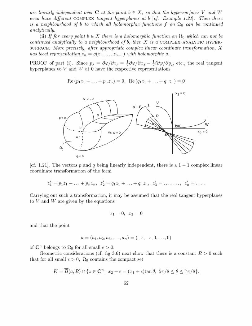
are linearly independent over C at the point b ∈ X, so that the hypersurfaces V and Weven have different complex tangent hyperplanes at b [cf. Example 1.21]. Then thereis a neighbourhood of b to which all holomorphic functions f on Ω0 can be continuedanalytically.

(ii) If for every point b ∈ X there is a holomorphic function on Ω0 which can not becontinued analytically to a neighbourhood of b, then X is a complex analytic hyper-surface. More precisely, after appropriate complex linear coordinate transformation, Xhas local representation zn = g(z1, . . . , zn−1) with holomorphic g.

PROOF of part (i). Since pj = ∂ϕ/∂zj = 12∂ϕ/∂xj − 1

2 i∂ϕ/∂yj, etc., the real tangenthyperplanes to V and W at 0 have the respective representations

Re (p1z1 + . . .+ pnzn) = 0, Re (q1z1 + . . .+ qnzn) = 0

a

b=0 W

V

x1 = 0

a + E 1

R

x2 = 0

k

x

V: φ = 0

W: ψ = 0

φ < 0

ψ < 0

Ω0

a x

X

b

fig 3.5 fig 3.6[cf. 1.21]. The vectors p and q being linearly independent, there is a 1− 1 complex linearcoordinate transformation of the form

z′1 = p1z1 + . . .+ pnzn, z′2 = q1z1 + . . .+ qnzn, z

′3 = . . . , . . . , z′n = . . . .

Carrying out such a transformation, it may be assumed that the real tangent hyperplanesto V and W are given by the equations

x1 = 0, x2 = 0

and that the point

a = (a1, a2, a3, . . . , an) = (−ε,−ε, 0, . . . , 0)

of Cn belongs to Ω0 for all small ε > 0.Geometric considerations (cf. fig 3.6) next show that there is a constant R > 0 such

that for all small ε > 0, Ω0 contains the compact set

K = B(a,R) ∩ z ∈ Cn : x2 + ε = (x1 + ε)tan θ, 5π/8 ≤ θ ≤ 7π/8.

62

Observe that the corresponding real “directions” or unit vectors ξ = (ξ1, ξ2, . . . , ξn) withξ2 = ξ1 tan θ, 5π/8 < θ < 7π/8 form a nonempty open subset E of the unit sphere Sn−1

in Rn.Now let f be in O(Ω0), supK |f | = C = C(f,K). Any complex line L through a of

the form z = a+ wξ, ξ ∈ E intersects K in a disc ∆ of radius R. The restriction of f to∆ is represented by the function

h(w) = f(a+ wξ), |w| ≤ R.

Applying the Cauchy inequalities to h on ∆1(0, R) we find that

(5a)1

m!

∣

∣

∣

∣

(

d

dw

)m

f(a+ wξ)∣

∣

w=0

∣

∣

∣

∣

≤ C

Rm, ∀ξ ∈ E, ∀m ∈ N0.

Hence by the partial derivatives lemma, considering the restriction of f to Ω0 ∩Rn andtaking w = t ∈ R,

(5b) max|α|=m

1

α!

∣

∣Dαx f(a)

∣

∣ ≤ C/(βR)m, ∀m; β = β(E) > 0.

Since f is analytic on Ω0, the derivatives Dαz f(a) are equal to the derivatives Dα

x f(a).Thus around a,

f(z) =∑

cα(z − a)α =∑

α≥0

1

α!Dαx f(a) (z1 − a1)α1 . . . (zn − an)αn .

By (5b), the power series will converge at every point z with |zj − aj| < βR, ∀j :

∣

∣cα(z − a)α∣

∣ ≤ C∣

∣

∣

∣

z1 − a1

βR

∣

∣

∣

∣

α1

. . .

∣

∣

∣

∣

zn − anβR

∣

∣

∣

∣

αn

, ∀α.

Conclusion: f has an analytic continuation to the polydisc ∆(a, βR) and in fact,letting ε ↓ 0 so that a→ 0, to the polydisc ∆(0, βR).

REMARK on part (ii). The crucial observation is that under the hypothesis of part (ii),the complex tangent hyperplanes to V and W must coincide along X. As a consequence,the (2n − 2)-dimensional real tangent spaces to X are complex hyperplanes. This beingthe case, one may conclude that X is complex analytic (“Levi-Civita lemma”). For moredetailed indications of the proof, see exercise 3.19.

3.6 The edge-of-the-wedge theorem. We will discuss a simple version for Cn andbegin with the special case n = 1 in order to bring out more clearly why the theorem is soremarkable for n ≥ 2. Let W+ be a(n open) rectangular domain in the upper half-plane inC, of which one side falls along the real axis. The reflected rectangle in the lower half-planeis called W− and the (open) common boundary segment is called H (fig 3.7). We finallyset

W = W+ ∪H ∪W−.

63

W+

W-

z

z

Γ

Γ

RH

_x

x

fig 3.7

For n = 1 our simple edge-of-the-wedge theorem reduces to the following well-known facts:

(i) (A segment as removable singularity set). Any continuous function f on W whichis holomorphic on W+ and on W− is actually holomorphic on W.

[The integral of fdz along any piecewise smooth simple closed curve Γ in W will bezero, cf. fig 3.7, hence f is analytic on W . One may appeal to Morera’s theorem here, orobserve directly that f will have a well-defined primitive F (z) =

∫ z

af(ζ)dζ on W. Since F

is differentiable in the complex sense, it is analytic, hence so is f = F ′.]

(ii) (Analytic continuation by Schwarz reflection). Any continuous function g on

W+ ∪H which is holomorphic on W+ and real-valued on H has an analytic continuationto W. For z ∈W− the continuation is given by reflection: g(z) = g(z).

[Apply part (i) to the extended function g. The condition that g (or f in part (i)) becontinuous at the points of H can be weakened, cf. [Carleman] and Remarks 3.62.

the case of Cn (n ≥ 1). Let H (for “horizontal”) be a connected domain in the real spaceRn = Rn + i0 in Cn and let V (for “vertical”) be a (usually truncated) connected opencone with vertex at the origin in (another) Rn. To get a simple picture, we assume thatV and −V meet only at the origin. To H and V we associate two (connected) domains inCn as follows:

W+ = H + iV = z = x+ iy ∈ Cn : x ∈ H, y ∈ V , W− = H − iV

(“wedges” with common “edge” H). We again define

W = W+ ∪H ∪W−.

Observe that W is not an open set when n ≥ 2: W does not contain a Cn neighbourhood ofany point a ∈ H (fig 3.8). For n ≥ 2, the set H is a peculiarly small part of the boundaryof W+: it only has real dimension n instead of 2n− 1, as one would expect of a “normal”piece of the boundary of a Cn domain. For the purpose of illustration when n = 2, onlyone line segment of H has been drawn in fig 3.9. In that way one clearly sees two wedgeswith a common edge.

64

a

a + iV

a - iV

HW+

W-

H

a

z = a +wξ

D

fig 3.8 fig 3.9

Theorem 3.61. Let H, V, W+, W− and W be as described above. Then there exists aconnected domain D in Cn containing W such that the following is true:

(i) Any continuous function f on W which is holomorphic on W+ and on W− hasan analytic continuation to D;

(ii) Any continuous function g on W+ ∪ H which is holomorphic on W+ and real-valued on H has an analytic continuation to D; for z ∈W−, the continuation is given byreflection: g(z) = g(z).

REMARKS 3.62. For every point a ∈ H there will be a fixed Cn neighbourhood to whichall functions f and g as in the Theorem can be analytically continued. Actually, thehypothesis that f ∈ O(W+ ∪ W−) has a continuous extension to W can be weakenedconsiderably. It is sufficient if for y → 0 in V , the function

Fy(x) = f(x+ iy)− f(x− iy), x ∈ H ⊂ Rn

tends to 0 in weak or distributional sense ([Bogolyubov-Vladimirov], cf. [Rudin 4], [Kore-vaar 1991]; weak convergence is defined in Chapter 11). It even suffices to have convergencehere in the sense of hyperfunctions [De Roever]. There are several forms of the edge-of-the-wedge theorem and many different proofs have been given, cf. [Rudin 4] and [Shabat].

PROOF of the Theorem. One need only consider part (i) since part (ii) will follow as inthe case n = 1. It is sufficient to show that there is a polydisc ∆(a, ρ), ρ = ρa aroundeach point a ∈ H to which all functions f as in part (i) can be continued analytically. Wefocus on one such function f . The key observation will be that W contains closed squaresQξ(a) of constant size with center a in a substantial family of complex lines (cf. fig 3.9):

z = a+ wξ, ξ ∈ E ⊂ Sn−1 ⊂ Rn, w = u+ iv ∈ C.

By the one-variable result, the (continuous) restrictions f |Qξ(a) are analytic. The Cauchyinequalities now imply bounds on certain directional derivatives of f |H. Such bounds (atand around a) and the partial derivatives lemma will ensure that f |H is locally repre-sented by a power series

∑

cα(x − a)α; replacing x by z one obtains the desired analyticcontinuation.

65

Let us first look at V . The directions from 0 that fall within the cone V determine anonempty open subset E′ of the unit sphere Sn−1. We choose some open subset E withcompact closure in E′. There will then be a number R > 0 such that V ∪ 0 contains theclosed truncated cone

V0 = y ∈ Rn : y = vξ, ξ ∈ E, 0 ≤ v ≤ R.

For a ∈ H, the domain H ⊂ Rn contains the real ball U(a, d) : |x − a| < d = d(a, ∂H).Choosing R < d, our set W will contain the squares

Qξ(a) = z ∈ Cn : z = a+ wξ, ξ ∈ E, −R ≤ u, v ≤ R.

The union of these squares for ξ running over E is a compact subset of W [contained inU(a,R)± iV0], on which |f | will be bounded, say by C = Cf .

The restriction of f to Qξ(a) is represented by

h(w) = f(a+ wξ), −R ≤ u, v ≤ R.

The function h is continuous on its square and analytic for v = Imw 6= 0, hence it isanalytic on the whole square. Thus as in Section 3.5, the Cauchy inequalities give a familyof inequalities (5a). Here C and R (may) depend on a, but if we fix b in H and restrict ato a small neighbourhood H0 of b in H, we may take Cf and R constant.

The inequalities (5a), with w = t ∈ R and a running over H0, will imply thatf0 = f |H0 is of class C∞ around b and that it has a holomorphic extension f to a Cn

neighbourhood of b. We sketch a proof; another proof may be derived from exercise3.23. Choose a convex neighbourhood H1 of b in H0 such that d(H1, ∂H0) = δ > 0.Now “regularize”f0 through convolution with the members of the approximate identityρε of (3a, b), 0 < ε < δ. One thus obtains C∞ functions fε = f0 ? ρε on H1 whosederivatives in the directions ξ ∈ E satisfy the inequalities (5a) (with w = t ∈ R) for alla ∈ H1 and all ε ∈ (0, δ). By the partial derivatives lemma, the derivatives Dα

x of thefunctions fε will then satisfy the inequalities (5b) for every a ∈ H1. Taylor’s formula withremainder next shows that the real Taylor series for fε with center a ∈ H1 converges tofε on ∆(a, βR) ∩ H1. Complexifying such Taylor series for fε, one obtains holomorphicextensions fε of the functions fε to the union D1 of the polydiscs ∆(a, βR) with a ∈ H1.[H1 is a set of uniqueness for D1, cf. exercise 1.17.] The family fε, 0 < ε < δ will belocally bounded on D1 and fε → f0 on H1 as ε ↓ 0. Thus by Vitali’s theorem 1.74, thefunctions fε converge to a holomorphic extension f of f0 on D1.

Since f = f0 = f on H1, f will also agree with f on the intersection of D1 with anycomplex line z = a + wξ for which a ∈ H1 and ξ ∈ E. It follows that f = f throughoutopen subsets of W+ and W−. Conclusion: f provides an analytic continuation of f to D1

and in particular, to the polydisc ∆(a, βR) for every a ∈ H1.

Exercises

66

3.1. (Direct verification of the representation (1e)) Let a be fixed and z variable in C, z =a+ reiθ. Let f be a C1 function on C of compact support. Prove that

∂f

∂z=

1

2eiθ(

∂f

∂r− 1

ir

∂f

∂θ

)

and deduce that for ε ↓ 0 :

∫

|z−a|>ε

∂f

∂z

1

z − adxdy = −1

2

∫ π

−π

f(a+ εeiθ)dθ → −πf(a).

3.2. Extend formula (1e) to arbitrary functions f in C1(C) which tend to 0 as |z| → ∞while |∂f/∂z|/|z| is integrable over C.

3.3. Why can not one calculate ∂u/∂z by differentiation under the integral sign in formula(1f) as it stands?

3.4. Prove a formula for (∂u/∂y)(a) analogous to (1i), starting with an appropriate analogto (1h).

3.5. Let v ∈ C(C) be of compact support and let u be its Cauchy-Green transform (1f).Prove that u is holomorphic outside supp v. Expand u in a Laurent series around∞ toobtain conditions on the “moments”

∫

Cv(ζ)ζkdξdη which are necessary and sufficient

in order that u vanish on a neighbourhood of ∞.3.6. Let v be a continuous function on C of compact support and let u be its Cauchy-Green

transform (1f). Prove that u is of class Lipα for each α ∈ (0, 1) or even better, that

|u(z + h)− u(z)| ≤M |h| log (1/|h|)

for some constant M and all z ∈ C, all |h| ≤ 12 . [Take 0 < |h| ≤ 1

2 , ζ ∈ supp v ⊂B(0, R) for some R ≥ 1, |z| ≤ 2R. Substituting ζ − z = hζ ′, the variable ζ ′ may berestricted to the disc B(0, 3R/|h|).]

3.7. Let D ⊂ C be a domain as in Proposition 3.11 and let v be of class C1(D). Supposeone knows that the equation ∂u/∂z = v has a solution f on D which extends to a C1

function on D. Prove that

u(z)def= − 1

π

∫

D

v(ζ)

ζ − z dξdη, ζ = ξ + iη

is also a C1 solution on D.

3.8. (Continuation) Let D be as in Proposition 3.11 and let v be continuous on D. Provethat the Cauchy-Green transform u of v on D (exercise 3.7) is also continuous andthat it provides a weak solution of the equation ∂u/∂z = v on D. That is,

〈∂u∂z, ϕ〉 def

= −〈u, ∂ϕ∂z〉 def

= −∫

D

u∂ϕ

∂zdxdy

67

is equal to

〈v, ϕ〉 def=

∫

D

vϕ dxdy

for all test functions ϕ on D (all C∞ functions ϕ of compact support in D). [If vbelongs to C1(D) the function u will be an ordinary solution, cf. Section 11.2.]

3.9. Verify that the function u(z) in formula (2c), with v as in Proposition 3.21, is of classCp as a function of x1, y1, . . . , xn, yn. Next use the method of exercise 3.6 to show thatthe partial derivatives of u of order p are of class Lipα, ∀α ∈ (0, 1).

3.10. Verify that the functions σ and τ introduced in Section 3.3 are of class C∞ on R.

3.11. Verify that the functions ρε of (3a, b) constitute a C∞ approximate identity on Rn asε ↓ 0.

3.12. Let ω be the cutoff function of (3c) and let e1 denote the unit vector in the x1 direction.Prove that

∂ω

∂x1(a) = lim

h→0

ω(a+ he1)− ω(a)

hexists and =

∫

Sε

∂ρε∂x1

(a− y)dy.

3.13. Let u be continuous on Rn and let ρε be a C∞ approximate identity with supp ρε ⊂B(0, ε). Prove that the “regularization” uε = u ? ρε is of class C∞ and that uε → u asε ↓ 0, uniformly on every compact subset of Rn.

3.14. (Weak solutions of Du = 0 are holomorphic) Let u be continuous on C and such that∂u/∂z = 0 in the weak sense, cf. exercise 3.8. Prove that u is holomorphic. [Showfirst that ∂uε/∂z = 0, where uε is as in exercise 3.13.]

3.15. Show by an example that there is no Hartogs-Osgood-Brown continuation theoremfor n = 1. Where does the proof of Theorem 3.41 break down when n = 1?

3.16. Let D be a simply connected domain in C, K ⊂ D a compact subset such thatD−K is connected. Prove that a holomorphic function f on D−K can be continuedanalytically to D if and only if

∫

Γf(ζ)/(ζ − z)dζ = 0 for some [and then for every]

piecewise smooth simple closed curve Γ around K in D −K and for all z outside Γ.

3.17. (Continuation) Prove that the following moment conditions are also necessary andsufficient for the possibility of analytic continuation of f across K :

∫

Γf(ζ)ζkdζ =

0, ∀k ≥ 0 for some curve Γ as above.

3.18. Prove that every holomorphic function on the domain D = z = x + iy ∈ C2 :min(x1, x2) < 0 has an analytic continuation to all of C2.

3.19. (Proof of Theorem 3.52 part (ii)) Let V, W, Ω0 and X satisfy the hypotheses of The-orem 3.52 part (ii). Verify the following assertions:(i) At every point b ∈ X, the hypersurfaces V and W have the same complex tangent

hyperplane.(ii) The real tangent spaces to X are complex hyperplanes.

68

(iii) The real tangent hyperplanes to V and W at b ∈ X being different, one has∂ψ/∂zj = λ∂ϕ/∂zj at b, j = 1, . . . , n, with λ = λ(b) nonreal.

(iv) Supposing from here on that ∂ϕ/∂zn 6= 0 at the point b ∈ X, the vectors(∂ϕ/∂xn, ∂ϕ/∂yn) and (∂ψ/∂xn, ∂ψ/∂yn) are linearly independent at b.

(v) By real analysis, X has a local representation zn = xn + iyn = g(z′) =g(z1, . . . , zn−1) around b. [Cf. Remarks 5.13.]

(vi) The function g satisfies the Cauchy-Riemann equations around b′. [Cf. assertion(ii) above.]

3.20. Let H = R2, let V be the positive “octant” y1 > 0, y2 > 0 of (another) R2 and setW = (H + iV )∪H ∪ (H − iV ) in C2. Which points z = a+ iy near a ∈ H are outsideW? [Cf. fig 3.8.]

3.21. (Continuation) Prove that any function f which is continuous on W and analytic onW+ and W− has an analytic continuation to all of C2.

3.22. Let f0 be a continuous function on the domain H0 ⊂ Rn which possesses derivativesof all orders in the directions ξ ∈ E throughout H0. Suppose that these derivativessatisfy the inequalities (5a) with w = t ∈ R at all points a ∈ H0. Let H1 be asubdomain of H0 such that d(H1, ∂H0) = δ > 0 and let ρε be the approximateidentity of (3a, b), with 0 < ε < δ. Prove that the regularizations fε = f0 ? ρε satisfythe inequalities (5a) (with w = t) at every point a ∈ H1.

3.23. Let f be a continuous function on a domain H in Rn such that for n linearly indepen-dent unit vectors ξ and every m ≥ 1, the directional derivatives (d/dt)mf(x+ tξ)|t=0

exist and are bounded functions on a neighbourhood H0 of each point b ∈ H. Provethat f is of class C∞. [By a linear coordinate transformation it may be assumed thatthe unit vectors ξ are equal to e1, . . . , en. Multiplying f by a C∞ cutoff function withsupport in H0 which is equal to 1 around b, one may assume that f has its supportin the hypercube −π < x1, . . . , xn < π. Taking n = 2 for a start, one knows thatDm

1 f and Dm2 f exist and are bounded for m = 1, 2, . . . . Introducing the Fourier series

∑

cpq expi(px1 + qx2) for f on the square −π < x1, x2 < π, one may conclude thatthe multiple sequence (|p|m + |q|m)cpq, (p, q) ∈ Z2 is bounded for each m. Deducethat the (formal) series for Dαf is uniformly convergent for every α, hence ... .]

3.24. (Alternative proof of 3.61) We adopt the notation of 3.6..i. Show that we may assume that H contains the cube |xi| < 6 and that V contains

the truncated cone 0 < vi < 6 and that assuming this, it suffices to show that fextends to the unit polydisc ∆ = ∆(0, 1).

ii. Let c =√

2− 1 and let φ(w, λ) = w+λ/c1+cλw

. Check the following:a. If |λ| = 1 or w is real, then Imφ.Imλ ≥ 0.b. |φ| < 6 for |λ|, |w| < 1.c. φ(w, 0) = w.

iii. FormΦ(z, λ) = (φ(z1, λ), . . . , φ(zn, λ)

and consider gz(λ) = f(Φ(z, λ)). Show that gz is well defined for z ∈ H ∩ ∆,|λ| ≤ 1 and for |λ| = 1 and z ∈ ∆. Show that for z ∈ H ∩∆, gz(λ) is analytic on

69

|λ| < 1. Use Corr.1.72 to see that

F (z) :=

∫ π

−π

gz(eiθ)dθ

2π

is analytic on ∆.iv. Show that for z ∈ H ∩∆ one has F (z) = gz(0) = f(z).v. Show that F is an analytic extension of f to ∆.

70

CHAPTER 4

Local structure of holomorphic functions

Zero sets and singularity sets

We will study germs of holomorphic functions at a point a. These germs form a ringOa, addition and multiplication being defined by the like operations on representatives.One loosely speaks of the ring of holomorphic functions at a.

For the study of O0 in Cn, it is customary to single out one of the variables. In thefollowing this will be zn; we denote (z1, . . . , zn−1) by z′, so that

z = (z1, . . . , zn−1, zn) = (z′, zn), z′ ∈ Cn−1, zn ∈ C.

We similarly split the radii of polydiscs ∆(0, r) ⊂ Cn :

r = (r1, . . . , rn−1, rn) = (r′, rn), rj > 0.

In this context the origin of Cn−1 will usually be called O′.Suppose now that f is holomorphic in some unspecified neigbourhood of 0 in other

words: [f ] ∈ O0 and that f(0) = 0, f 6≡ 0. In the case n = 1 the local structure of f and thelocal zero set Zf are very simple: in a suitably small neighbourhood of 0, the function f(z)can be written as E(z)zk, where k ≥ 1 and E is zero free in a neighbourhood of 0. In thecase n ≥ 2 the origin can not be an isolated zero of f , but the fundamental weierstrasspreparation theorem (Section 4.4) will furnish a related factorization. After an initiallinear transformation which favors the variable zn, one obtains a local representation

f(z) = E(z)W (z)

on some small neighborhood of 0, that is [f ] = [E][W ] in O0. Here W is a so-calledWeierstrass polynomial in zn and E is zero free and holomorphic in some neighbourhoodof the origin. This means: W is a polynomial in zn with leading coefficient 1; the othercoefficients are analytic in z′ = (z1, . . . , zn−1) near 0′ and they vanish at 0′. Around 0, Wwill have the same zero set as f and this fact prepares the way for further study of Zf .

The detailed investigation of ZW will be based on a study of the polynomial ringO′

0[zn], where O′0 stands for the ring O0 in Cn−1 (Sections 4.5, 4.6).

After we have obtained a good description of the zero set, it becomes possible to provesome results on removable singularities. We will also see that certain “thin” singularitysets are at the same time zero sets.

Normalization relative to zn and a basic auxiliary result. Let f be holomorphic ina neighbourhood of the origin in Cn. In the (absolutely convergent) power series

∑

cαzα

for f(z) around 0, we may collect terms of the same degree:

(1a)

f(z) = P0(z) + P1(z) + P2(z) + . . . ,

Pj(z) =∑

|α|=j

cαzα homogeneous in z1, . . . , zn of degree j.

71

DEFINITION 4.11. The function f is said to vanish (exactly) of order k ≥ 1 at the originif

Pj ≡ 0, j = 0, . . . , k − 1; Pk 6≡ 0.

An equivalent statement would be [cf. Section 1.5]:

Dαf(0) = Dα1

1 . . .Dαnn f(0) = 0, ∀α with |α| = α1 + . . .+ αn < k,

Dβf(0) 6= 0 for some β with |β| = k.

DEFINITION 4.12. The function f is said to be normalized relative to zn at the originif f(0′, zn) does not vanish identically in a neighbourhood of zn = 0. Such an f is saidto vanish (exactly) of order k relative to zn at the origin if f(0′, zn) has a zero of order(exactly) k for zn = 0. Equivalently:

Djnf(0) = 0, j = 0, . . . , k − 1; Dk

nf(0) 6= 0.

Corresponding definitions apply at a point a ∈ Cn: one may consider f(a+z) insteadof f(z). If f is normalized relative to zn at 0 [so that Dk

nf(0) 6= 0, say], then f is alsonormalized relative to zn at all points a close to 0.

EXAMPLE 4.13. The function f(z) = z1z2 on C2 vanishes of order 2 at the origin. Itis not normalized relative to z2, but one can normalize it relative to the final variableby the substitution z1 = ζ1 + ζ2, z2 = ζ2. Then f goes over into the analytic functiong(ζ) = ζ1ζ2 + ζ2

2 which vanishes of order 2 relative to ζ2 at the origin.

Lemma 4.14. Suppose f vanishes (exactly) of order k at the origin. Then one can alwayscarry out a 1− 1 linear coordinate transformation z = Aζ in Cn to ensure that f vanishesof order (exactly) k at 0 relative to the (new) n-th coordinate.

PROOF. Write f as a sum of homogeneous polynomials of different degree as in (1a), sothat Pk 6≡ 0. Choose b 6= 0 such that Pk(b) 6= 0 and then construct an invertible n × nmatrix A with n-th column b. Now put z = Aζ and set

g(ζ)def= f(Aζ) = Pk(Aζ) + Pk+1(Aζ) + . . . .

Observe that A times the (column) vector (0, . . . , 0, ζn) equals (b1ζn, . . . , bnζn), so that

g(0, . . . , 0, ζn) = f(b1ζn, . . . , bnζn) = Pk(b1ζn, . . . , bnζn)+

+ Pk+1(. . .) + . . . = Pk(b)ζkn + Pk+1(b)ζk+1n + . . . .

Clearly Dkng(0) 6= 0.

72

Auxiliary Theorem 4.15. Let f be holomorphic on the polydisc ∆(0, r) ⊂ Cn, n ≥ 2and suppose that f vanishes (exactly) of order k relative to zn at the origin. Then thereexist a smaller polydisc ∆(0, ρ) :

0 < ρ = (ρ1, . . . , ρn−1, ρn) = (ρ′, ρn) < r = (r′, rn)

and a number ε > 0 such that

(1b) f(0′, zn) 6= 0 for 0 < |zn| ≤ ρn,

(1c) f(z′, zn) 6= 0 for z′ ∈ ∆n−1(0′, ρ′), ρn − ε < |zn| < ρn + ε(≤ rn).

For any z′ ∈ ∆(0′, ρ′), the function g(zn) = f(z′, zn) will have precisely k zeros in the disc∆1(0, ρn) (counting multiplicities).

PROOF. The function f(0′, zn) is holomorphic on the disc ∆1(0, rn) and it has a zeroof order k at zn = 0. Since the zeros of f(0′, zn) are isolated, there exists a numberρn ∈ (0, rn) such that f(0′, zn) 6= 0 for 0 < |zn| ≤ ρn.

The function f(z′, zn) is holomorphic and hence continuous on a Cn neighbourhoodof the circle

γ : z′ = 0′, |zn| = ρn.It is different from 0 on γ, hence 6= 0 on some Cn polydisc around each point (0′, w) ∈ γ.Covering γ by a finite number of such polydiscs ∆n−1(0′, s′)×∆1(w, sn), we conclude thatf(z′, zn) 6= 0 on a Cn neigbourhood of γ in ∆(0, r) of the form

∆n−1(0′, ρ′)× ρn − ε < |zn| < ρn + ε.

|zn|

εερn

(|z1|,...,|zn-1|)

0 ρ' fig 4.1We now fix z′ ∈ ∆(0′, ρ′) for a moment. The function g(w) = f(z′, w) is holomorphic

on the closed disc ∆1(0, ρn) and zero free on the circumference C(0, ρn). The number ofzeros Ng = N(z′) of g in ∆1(0, ρn) (counting multiplicities) may be calculated with theaid of the residue theorem:

(1d) N(z′) = Ng =1

2πi

∫

C(0,ρn)

g′(w)

g(w)dw =

1

2πi

∫

C(0,ρn)

∂f(z′, w)/∂w

f(z′, w)dw.

73

[Cf. Section 1.8. For any holomorphic h(w), the residue of hg′/g at a µ-fold zero w0 of gwill be µh(w0).]

With formula (1d) in hand, we let z′ vary over ∆(0′, ρ′). The final integrand is contin-uous in (z, w) on ∆(0′, ρ′)× C(0, ρn) [which is a subset of ∆(0, r)], since the denominatorf(z′, w) does not vanish there [see (1c)]. Furthermore, the integrand is holomorphic inz′ for each w on C(0, ρn). Applying the holomorphy theorem for integrals 1.72 [cf. alsoSection 2.6], it follows that N(z′) is holomorphic on ∆(0′, ρ′). Since N(z′) is integer-valued,it must be constant, hence

N(z′) = N(0′) = k,

the number of zeros of f(0′, w) or f(0′, zn) in ∆1(0, ρn) [always counting multiplicities].

4.2 An implicit function theorem. Let f, r and ρ be as in Auxiliary Theorem 4.15 sothat in particular f is holomorphic on ∆(0, ρ). Supposing that k = 1, the equation

g(w) = f(z′, w) = 0 [with arbitrary fixed z′ in ∆(0′, ρ′)]

has precisely one root w = w0 = ϕ(z′) inside the disc ∆1(0, ρn) [and no root on theboundary C(0, ρn)]. With the aid of the residue theorem we can represent this root by anintegral similar to (1d) :

(2) ϕ(z′) = w0 =1

2πi

∫

C(0,ρn)

wg′(w)

g(w)dw =

1

2πi

∫

C(0,ρn)

w∂f(z′, w)/∂w

f(z′, w)dw.

Letting z′ vary over ∆(0′, ρ′), this integral shows that ϕ(z′) is holomorphic, cf. the pre-ceding proof. The result is important enough to be listed as a theorem:

Theorem 4.21 (implicit function theorem). Let f be holomorphic on the polydisc∆(0, r) ⊂ Cn and suppose that f vanishes (exactly) of order 1 relative to zn at the origin:

f(0) = 0, Dnf(0) 6= 0.

0

x

(z’,0)

zn-plane

(z’,φ(z’))

ρ’

z’-space

ρn

fig 4.2Then there exists ρ = (ρ′, ρn) with 0 < ρ < r such that on the polydisc ∆(0′, ρ′) ⊂

Cn−1, there is a unique holomorphic function ϕ(z′) with the following properties:(i) ϕ(0′) = 0,(ii) ϕ(z′) ⊂ ∆1(0, ρn), ∀z′ ∈ ∆(0′, ρ′),

74

(iii) f(z′, zn) = 0 at a point z ∈ ∆(0, ρ) if and only if zn = ϕ(z′) with z′ ∈ ∆(0′, ρ′).

COROLLARY 4.22. Let f be holomorphic on D ⊂ Cn and vanish (exactly) of order1 at the point a ∈ D. Then there is a neighbourhood of a in which the zero set Zf ishomeomorphic to a domain in Cn−1. [In this case a is called a regular point of Zf . Sincehomeomorphisms preserve dimension, the zero set has complex dimension n − 1 or realdimension 2n− 2.]

Indeed, taking a = 0 and normalizing relative to zn as in Lemma 4.14, we will havef(0) = 0, Dnf(0) 6= 0. By Theorem 4.21 there is then a polydisc ∆(0, ρ) ⊂ D in which Zfhas the form

Zf ∩∆(0, ρ) = (z′, φ(z′)) ∈ Cn : z′ ∈ ∆(0′, ρ′)with ϕ ∈ O(∆(0′, ρ′)). The correspondence z′ ↔ (z′, ϕ(z′)) between ∆(0′, ρ′) and Zf (thegraph of ϕ) in ∆(0, ρ) is 1− 1 and bicontinuous.

In the following sections we will investigate the zero set in the vicinity of a point wheref vanishes of order > 1.

4.3 Weierstrass polynomials. Let f, r and ρ again be as in Auxiliary Theorem 4.15,so that in particular f is holomorphic on ∆(0, ρ). Taking k ≥ 1 arbitrary this time, theequation

(3a) g(w) = f(z′, w) = 0 [with arbitrary fixed z′ in ∆(0′, ρ′)]

has precisely k roots inside the disc ∆1(0, ρn), counting multiplicities [and no root on theboundary C(0, ρn)]. We may number the roots in some order or other:

(3b) w1 = w1(z′), . . . , wk = wk(z′); wj(0′) = 0, ∀j.

However, occasionally some roots may coincide, and in general it is not possible to definethe individual rootswj(z

′) in such a way that one obtains smooth functions of z′ throughout∆(0′, ρ′). [Think of f(z′, w) = z1 − wk.]

In this situation it is natural to ask if the functions (3b) might be the roots of a nicealgebraic equation. Let us consider the product

(3c) (w − w1) . . . (w − wk) = wk +k∑

j=1

ajwk−j , aj = aj(z

′).

Apart from a ± sign, the coefficients aj are equal to the so-called elementary symmetricfunctions of the roots:

a1 = −(w1 + . . .+ wk), a2 = w1w2 + . . .+ w1wk + w2w3 + . . .+ wk−1wk, . . . ,

ak = (−1)kw1 . . .wk.

Observe that aj(0′) = 0, j = 1, . . . , k. We will show that the coefficient aj(z

′) dependanalytically on z′. The proof may be based on an algebraic relation between symmetricfunctions (to be found in [Van der Waerden] for example) of which we will give an analyticproof.

75

Lemma 4.31. The coefficients aj = aj(z′) in (3c) can be expressed as polynomials in the

power sumssp = sp(z

′) = wp1 + . . . wpk, p = 1, 2, . . .

and (hence) they are holomorphic functions of z′ on ∆(0′, ρ′).

PROOF. (i) it is convenient to divide by wk in (4.33) and to set 1/w = t. Thus

Πkν=1(1− wνt) =

k∑

j=0

ajtj def

= P (t), a0 = 1.

Taking the logarithmic derivative of both sides and multiplying by t, one obtains the twoanswers

tP ′(t)

P (t)=

∑kj=1 jajt

j/∑km=0 amt

m,

∑kν=1

−wν t1−wνt

= −∑kν=1

∑∞p=1w

pνtp = −∑∞

p=1 sptp.

We now multiply through by the first denominator and find:

k∑

1

jajtj = −

k∑

0

amtm

∞∑

1

sptp.

Equating coefficients of like powers of t on both sides, the result is

(3d) jaj = −(aj−1s1 + aj−2s2 + . . .+ a0sj), j = 1, . . . , k.

Hence by induction, aj can be expressed as a polynomial in s1, . . . , sj.(ii) We complete the proof of the Lemma by showing that the power sums sp(z

′) areholomorphic in z′ on ∆(0′, ρ′). To this end we write sp(z

′) as an integral: by the residuetheorem, cf. (1d),

(3e) sp(z′) =

k∑

ν=1

wpν =1

2πi

∫

C(0,ρn)

wpg′(w)

g(w)dw =

1

2πi

∫

C(0,ρn)

wp∂f(z′, w)/∂w

f(z′, w)dw.

The holomorphy now follows as usual from the holomorphy theorem for integrals 1.72.The polynomial (3c) is called the Weierstrass polynomial belonging to the roots

w1, . . . , wk of the equation f(z′, w) = 0. Replacing w by zn we formulate:

Definition 4.32. A weierstrass polynomial in zn of degree k is a holomorphic func-tion in a neighbourhood of the origin in Cn of the special form

(3f) W (z′, zn) = zkn +

k∑

j=1

aj(z′)zk−jn , (k ≥ 1)

76

where the coefficients aj(z′) are holomorphic in a neighbourhood of 0′ in Cn−1 and such

that aj(0′) = 0, j = 1, . . . , k.

An arbitrary polynomial in zn with coefficients that are holomorphic in z′ is called a(holomorphic) pseudopolynomial in zn.

4.4 The Weierstrass theorems. Let f, r and ρ be as in Auxiliary Theorem 4.15, sothat in particular f is holomorphic on ∆(0, ρ). Moreover, the equation f(z′, w) = 0 withz′ fixed in ∆(0′, ρ′) has precisely k roots (3b) inside the disc ∆1(0, ρn) and no roots on theboundary C(0, ρn). Dividing g(w) = f(z′, w) by the Weierstrass polynomial W (w) (3c)with these same roots, we obtain a zero free holomorphic function E(w) on the closed disc∆1(0, ρn). Explicitly reintroducing z′, we have

(4a)f(z′, zn)

W (z′, zn)= E(z′, zn), (z′, zn) ∈ ∆n−1(0′, ρ′)×∆1(0, ρn).

Here E(z′, zn) is holomorphic in zn on ∆1(0, ρn) for each z′ ∈ ∆(0′ρ′). Also, E(z′, zn) isdifferent from 0 throughout δ(0′, ρ′)×∆1(0, ρn).

We will show that E is holomorphic in z = (z′, zn) on ∆(0, ρ). For this we use theone-variable Cauchy integral formula, initially with fixed z′ :

(4b) E(z) = E(z′, zn) =1

2πi

∫

C(0,ρn)

f(z′, w)

W (z′, w)

dw

w − zn, z = (z′, zn) ∈ ∆(0, ρ)

The holomorphy of E(z) now follows from the holomorphy theorem for integrals 1.72.Indeed, the integrand is continuous in (z, w) = (z′, zn, w) on ∆(0, ρ) × C(0, ρn) sinceW (z′, w)(w − zn) is different from zero there. Furthermore, for each w ∈ C(0, ρn),the integrand is holomorphic being a product of holomorphic functions in z′ and zn on∆(0′, ρ′)×∆1(0, ρn). Conclusion from (4a, b) :

Theorem 4.41 ( weierstrass’s preparation theorem). Let f be holomorphic on aneighbourhood of the origin in Cn. Suppose f vanishes at 0 (exactly) of order k relativeto zn. Then there is a neighbourhood of the origin in which f has a unique holomorphicfactorization

f(z) = E(z)W (z′, zn),

where W is a Weierstrass polynomial in zn of degree k (3f) and E is zero free.

The factorization is unique because W is uniquely determined by f . For the localstudy of zero sets one may apparently restrict oneself to Weierstrass polynomials. Thequestion of further decomposition of such polynomials will be taken up in Section 4.5.

There is also a preparation theorem for C∞ functions, see [Malgrange].There is a second (somewhat less important) Weierstrass theorem which deals with the

division of an arbitrary holomorphy function F by a preassigned Weierstrass polynomial[division with remainder]:

77

Theorem 4.42 ( Weierstrass’s division theorem). Let F be holomorphic in a neigh-bourhood of the origin in Cn and let W be an arbitrary Weierstrass polynomial in zn ofdegree k (3f). Then F has a unique representation around 0 of the form

(4c) F = QW + R,

where Q is holomorphic and R is a (holomorphic) pseudopolynomial in zn of degree < k.

We indicate a proof. Assuming that F and W are holomorphic on ∆(0, r) we chooseρ < r such that W (z) 6= 0 for z′ ∈ ∆(0′, ρ′) and |zn| = ρn, cf. Auxiliary Theorem 4.15.Then Q may be defined by

4d Q(z)def=

1

2πi

∫

C(0,ρn)

F (z′, w)

W (z′, w)

dw

w − zn, z ∈ ∆(0, ρ).

One readily shows that Q and hence Rdef= F − QW are holomorphic on ∆(0, ρ) and that

R is a pseudopolynomial in zn of degree < k, cf. exercise 4.6. For the uniqueness of therepresentation, cf. exercise 4.7.

4.5 Factorization in the rings O0 and O′0[zn]. As indicated before, the symbol Oa or

Oa(Cn) denotes the ring of germs of holomorphic functions at a, or equivalently, allpowerseries

f(z) =∑

α≥0

cα(z − a)α =∑

α≥0

cα1...αn(z1 − a1)α1 . . . (zn − an)αn

in z1, . . . , zn with center a that have nonempty domain of (absolute) convergence [cf. Sec-tion 2.3].For [f ] and [g] in Oa one defines the sum [f ] + [g] = [f + g] and the product[f ][g] = [fg] via representatives f, g. Product and sum are well defined at least throughoutthe intersection of the domains of f and g and this intersection will contain a.

As seen above, in working with germs, one strictly speaking has to take representatives,work with these on suitably shrunken neighbourhoods and pass to germs again. Usuallythe real work is done on the level of the representatives, while the other parts of the procesare a little tiresome. To avoid the latter, we will write f ∈ Oa, indicating both a germ ata or a representative on a suitable neighborhood, or even its convergent power series at a.This will not lead to confusion. Obviously there will be no loss of generality by studyingO0 only.

The zero element in O0 is the constant function 0. There is also a multiplicativeidentity, namely, the constant function 1. The ring O0 is commutative and free of zerodivisors cf. exercise 1.20]. Thus O0 is an integral domain. A series or function f ∈ O0 hasa multiplicative inverse 1/f in O0 if and only if f(0) 6= 0; such an f is called a unit in thering. The nonunits are precisely the series or functions which vanish at the origin; theyform a maximal ideal. For factorizations “at” the origin (around the origin) and for thelocal study of zero sets, units are of little interest.

DEFINITION 4.51. An element f ∈ O0 different from the zero element is called reducible(in or over O0) if it can be written as a product g1g2, where g1 and g2 are nonunits of

78

O0. An element f 6= 0 is irreducible if for every factorization f = g1g2 in O0, at least onefactor is a unit.

In reducibility questions for O0 we may restrict ourselves to Weierstrass polynomials,cf. the preparation theorem 4.41.

EXAMPLES. It is clear that z23 and z2

3 − z1z2z3 are reducible in O0(C3), but how about

(5a) W (z) = z23 − z2

1z2 ?

Proposition 4.52. Every (holomorphic) factorization of a Weierstrass polynomial intononunits of O0 is a factorization into Weierstrass polynomials, apart from units withproduct 1.

PROOF. Let W be a Weierstrass polynomial in zn of degree k (3f) and suppose thatW = g1g2, where the factors gj are holomorphic in a neighbourhood of 0 and gj(0) = 0.Setting z′ = 0′ we find

zkn = W (0′, zn) = g1(0′, zn)g2(0′, zn),

hence gj(0′, zn) 6≡ 0, so that the functions gj are normalized relative to zn at the origin

[Definition 4.12]. Thus we can apply the preparation theorem to each gj :

gj = EjWj , j = 1, 2

in some neighbourhood of 0. Here the Wj ’s are Weierstrass polynomials in zn and the Ej ’sare zero free. It follows that

W = 1 ·W = E1E2W1W2

in some neighbourhood of 0. Now W1W2 is also a Weierstrass polynomial in Zn and E1E2

is zero free. The uniqueness part of the preparation theorem thus shows that W1W2 = Wand E1E2 = 1.

We can now show that the Weierstrass polynomial (5a) is irreducible (over O0). Oth-erwise there would be a decomposition of the form

z23 − z2

1z2 = (z3 − w1(z′))(z3 − w2(z′))

with holomorphic functions wj at 0. This would imply w1+w2 = 0, w1w2 = −w21 = −z2

1z2,but the latter is impossible since z1

√z2 is not holomorphic at 0. [The function W of (5a)

is reducible over Oa for some points a where W (a) = 0 and a2 6= 0. Which precisely ?]

DEFINITION 4.53. An integral domain A with identity element is called a unique factor-ization domain (ufd) if every nonunit (6= 0) can be written as a finite product of irreduciblefactors in A and this in only one way, apart from units and the order of the factors.

79

PROPERTIES 4.54. Suppose A is a unique factorization domain. Then:

(i) The polynomial ring A[x] is also a ufd (“Gauss’s lemma”);

(ii) For any two relatively prime elements f and g in A[x] (that is, any nonzero f andg which do not have a nonunit as a common factor), there are relatively prime elementsS and T in A[x], with degreeS < degree g, degT < deg f , and a nonzero element R in Asuch that

(5b) Sf + Tg = R (“resultant of f and g”).

We indicate proofs, but refer to algebra books for details. For part (i) we need onlyconsider primitive polynomials f in A[x], that is, polynomials whose coefficients have nocommon factors others than units. By looking at degrees, it becomes clear that such f canbe decomposed into finitely many irreducible factors in A[x]. For the uniqueness one mayfirst consider the case where A is a (commutative) field. Then the Euclidean algorithmholds for the greatest common divisor (f, g) in A[x], hence (f1, g) = (f2, g) = 1 implies(f1f2, g) = 1. It follows that irreducible decompositions f = f1 . . . fr in A[x] must beunique. In the general case one first passes from A to the quotient field QA. A factorizationof f in A[x] gives one in QA[x]. For the converse, one observes that the product of twoprimitive polynomials in A[x] is again primitive. It follows that any factorization of f inQA[x] can be rewritten as a factorization into primitive polynomials in A[x]. Hence sinceAA[x] is a ufd, so is A[x].

As to part (ii), relatively prime elements f and g in A[x] are relatively prime in QA[x],hence by the Euclidean algorithm for the greatest common divisor, there exist S1 and T1

in QA[x], degS1 < deg g, degT1 < deg f such that S1f + T1g = 1. The most economicalremoval of the denominators in S1 and T1 leads to (5b).

Theorem 4.55. The rings O′0[zn] and O0 = O0(Cn) are unique factorization domains.

[Here O′0 stands for O0(Cn−1).]

PROOF. Concentrating on O0 we use induction on the dimension n. For n = 0 the ringO0 = C is a field and every nonzero element is a unit, hence there is nothing to prove.Suppose now that the theorem has been proved for O′

0 = O0(Cn−1). It then follows fromGauss’s lemma that the polynomial ring O′

0[zn] of the pseudopolynomials in zn is also aufd.

Next let f be an arbitrary nonunit 6= 0 inO0 = O0(Cn).By a suitable linear coordinatetransformation we ensure that f is normalized relative to zn, cf. Lemma 4.14. Weierstrass’spreparation theorem then gives a factorization f = EW , where E is a unit in O0 andW ∈ O′

0[zn] is a Weierstrass polynomial. As a consequence of the induction hypothesis,W can be written as a finite product of irreducible polynomials in O′

0[zn]. The factors areWeierstrass polynomials (apart from units with product 1) and they are also irreducibleover O0, cf. Proposition 4.52.

The uniqueness of the decomposition (apart from units and the order of the factors)follows by normalization from the uniqueness of the factorization f = EW at 0 and theuniqueness of the factorization in O′

0[zn].

80

Corollary 4.56 (irreducible local representation). Let f be holomorphic at 0 inCn and normalized relative to zn. Then f has a holomorphic product repesentation at 0[in a neighbourhood of 0] of the form

(5c) f = EW p11 . . .W ps

s .

Here E is zero free, the Wj’s are pairwise distinct irreducible Weierstrass polynomialsin zn and the pj ’s are positive integers. The representation is unique up to the order ofW1, . . . ,Ws.

We finally show that the rings O0(Cn) are Noetherian:

DEFINITION 4.57. A commutative ring A with identity element is called Noetherian ifevery ideal I ⊂ A is finitely generated, that is, if there exist elements g1, . . . , gk in I suchthat every f ∈ I has a representation f =

∑

ajgj with aj ∈ A.The so-called Hilbert basis theorem asserts that for a Noetherian ring A, the polyno-

mial ring A[x] is also Noetherian, cf. [Van der Waerden] section 84.

Theorem 4.58. O0 = O0(Cn) are Noetherian.

PROOF. One again uses induction on the dimension n. For n = 0 the ring O0 = C is afield, so that the only two ideals are the ones generated by 0 and by 1. Suppose, therefore,that n ≥ 1 and that the theorem has been proved for O′

0 = O0(Cn−1). Then by the aboveremark, the polynomial ring O′

0[zn] is also Noetherian.Now let I be any ideal in O0 = O0(Cn) which contains a nonzero element g. By change

of coordinates and the Weierstrass preparation theorem we may assume that g = EW ,where E is a unit in O0 and W is a Weierstrass polynomial in zn. Observe that W willalso belong to I and thus to the intersection J = I ∩ O′

0[zn].This intersection J is an ideal in the ring O′

0[zn], hence by the induction hypothesis, itis generated by finitely many elements g1, . . . , gp. We claim that in O0, the elements W andg1, . . . , gp will generate I. Indeed, let F be any element of I. By the Weierstrass divisiontheorem, F = QW + R, where Q ∈ O0 and R ∈ O′

0[zn]. Clearly R is also in I, henceR ∈ J , so that R = b1g1 + . . .+ bpgp with bj ∈ O′

0[zn]. Thus F = QW + b1g1 + . . .+ bpgp.

4.6 Structure of zero sets. We first discuss some global properties. Let f be a holo-morphic function 6≡ 0 on a connected domain D in Cn. What sort of subset is the zero setZf = Z(f) of f in D ?

Theorem 4.61. Zf is closed (relative to D) and thin: it has empty interior. The zero setdoes not divide D even locally: to every point a ∈ Zf there are arbitrarily small polydiscs∆(a, ρ) in D such that ∆(a, ρ)− Zf is connected. Ω = D − Zf is a connected domain.

PROOF. It is clear that Zf is closed [f is continuous] and that it has no interior points: iff would vanish on a small ball in D, it would have to vanish identically. [More generally,Zf can not contain a set of uniqueness 1.55 for O(D).]

Next let a be any point in Zf . We may assume that a = 0 and that f vanishes at 0 oforder k relative to zn. By Auxiliary Theorem 4.15, there will be arbitrarily small polydiscs∆(0, ρ) ⊂ D and ε > 0 such that f(0′, zn) 6= 0 for 0 < |zn| ≤ ρn and

f(z′, zn) 6= 0 throughout U = ∆(0′, ρ′)× ρn − ε < |zn| < ρn.

81

(b’,0)

(b’,c)

z’=b’

pts∈U

ρn

ρn - ε

pts∈Zfx

x x

x

fig 4.3Observe that the subset U ⊂ ∆(0, ρ)− Zf is connected. Furthermore, every point (b′, c)of ∆(0, ρ)− Zf may be connected to U by a straight line segment in ∆(0, ρ) lying in thecomplex plane z′ = b′ but outside Zf . Indeed, the disc z′ = b′, |zn| < ρn contains at mostk distinct points of Zf (fig 4.3). Thus ∆(0, ρ)− Zf is connected.

Any two point p and q in Ω can be joined by a polygonal path in D. Such a path maybe covered by finitely many polydiscs ∆(a, ρ) ⊂ D such that ∆(a, ρ) − Zf is connected.The latter domains will connect p and q in Ω.

We now turn our attention to the local form of Zf . We have already encounteredregular points of Zf , that is, points a around which Zf is homeomorphic to a domain inCn−1. Regularity of a point a ∈ Zf is assured if f vanishes at a of order exactly 1, seeCorollary 4.22.

Suppose from here on that f vanishes of order k at a, we may again take a = 0 andnormalize relative to zn to obtain the local irreducible representation (5c) for f . We willnow consider Zf purely as a set without regard to multiplicities. In that case it may beassumed that f is a Weierstrass polynomial in zn of the form

(6a) f = W1 . . .Ws,

where the factors are distinct and irreducible.

Theorem 4.62 (local form of the zero set). Let f be a Weierstrass polynomialin zn of degree k that is either irreducible or equal to a product (6a) of distinct irre-ducible Weierstrass polynomials W1, . . . ,Ws. Then there is a neighbourhood ∆(0, ρ) =∆(0′, ρ′) × ∆1(0, ρn) of the origin in Cn in which the zero set Zf may be described asfollows. There exists a holomorphic function R(z′) 6≡ 0 on ∆(0′, ρ′) such that for everypoint z′ in ∆(0′, ρ′) − ZR, there are precisely k distinct points of Zf in ∆(0, ρ) which lieabove z′; all those points are regular points of Zf . For z′ in ZR some roots of the equationf(z′, zn) = 0 in ∆1(0, ρn) will coincide. We say that the local zero set

Zf ∩∆(0, ρ)

is a k-sheeted complex analytic hypersurface above ∆(0′, ρ′) ⊂ Cn−1 which bran-ches (and can have nonregular points) only above the thin subset ZR of ∆(0′, ρ, ).

82

PROOF. The Weierstrass polynomial f in zn of degree k (6a) and its partial derivative

(6b)∂f

∂zn=

s∑

i=1

W1 . . .Wi−1∂W

∂znWi+1 . . .Ws

of degree k − 1 must be relatively prime in O′0[zn]. Indeed, none of the irreducible factor

Wj of f can divide ∂f/∂zn. This is so because Wj divides all the terms in the sum (6b)with i 6= j, but not the term with i = j: degree ∂Wj/∂zn < degWj .

The greatest common divisor representation (5b) for the ufd O′0[zn] now provides a

relation

(6c) Sf + T∂f

∂zn= R = R(z′)

relatively prime elements S and T in O′0[zn], degS < k − 1, degT < k, and a nonzero

element R(z′) in O′0. [A resultant R of f and ∂f/∂zn is also called a discriminant of f

as a pseudopolynomial in zn. The special case k = 1 is trivial, but fits in if we takeS = 0, T = 1 to yield R = 1.]

Relation (6c) may be interpreted as a relation among holomorphic functions on somepolydisc ∆(0, r). We now choose ∆(0, ρ) as in auxiliary theorem 4.15. For any pointb′ ∈ ∆(0′, ρ′), the equation

(6d) f(b′, zn) = 0

then has precisely k roots in ∆1(0, ρn), counting multiplicities. Suppose b′ is such thatsome of these roots coincide, in other words, equation (6d) has a root zn = c of multiplicity≥ 2. Then

(6e) f(b′, c) =∂f

∂zn(b′, c) = 0,

hence by (6c), R(b′) = 0.Conclusion: the k roots zn of the equation f(z′, zn) = 0 in ∆1(0, ρn) are all distinct

whenever R(z′) 6= 0 or z′ ∈ ∆(0′, ρ′) − ZR. The corresponding points (z′, zn) of Zf areregular: at those points ∂f/∂zn 6= 0 because of (6c); now see Corollary 4.22.

If R(b′) = 0, the k roots of (6d) must satisfy T∂f/∂zn = 0, hence if T (b′, zn) 6≡ 0, (6e)must hold for some c ∈ ∆1(0, ρn). However, even then (b′, c) may be a regular point of Zf :

EXAMPLE 4.63. For f(z) = z23 − z2

1z2 in O0(C3) we have ∂f/∂z3 = 2z3, hence

R(z′) = 2f(z)− z3∂f/∂z3 = −2z21z2

will be a resultant. The zero set Zf has two sheets over C2, given by z3 = ±z1√z2; the

sheets meet above ZR. The points of ZR have the forms z′ = (a, 0) and z′ = (0, b); the

83

corresponding points (a, 0, 0) and (0, b, 0) of Zf are of different character. Around (0, b, 0)with b 6= 0, Zf decomposes into two separate zero sets that meet along the complex linez1 = z3 = 0. However, the points (a, 0, 0) with a 6= 0 are regular for Zf , as is shown by thelocal representation z2 = z2

3/z21 !

Theorem 4.62 has various important consequences such as the so-called “Nullstellen-satz”, cf. exercises 4.17, 4.18.

ANALYTIC SETS 4.64. A subset X of a domain D ⊂ Cn is called an analytic set ifthroughout D, it is locally the set of common zeros of a family of holomorphic functions.[Since the rings Oa are Noetherian, one may limit oneself to finite families.] A point a ∈ Xis called regular if the intersection of X with a (small) polydisc ∆(a, r) is homeomorphicto a domain in a space Ck; the number k is called the complex dimension of X at a. BydimX one means the maximum of the dimensions at the regular points.

Taking D connected and f ∈ O(D), f 6≡ 0, the zero set Zf is an analytic set ofcomplex dimension n − 1. The set of the nonregular points of Zf is locally containedin the intersection of the zero sets of two relatively prime holomorphic functions, in thepreceding proof, f and ∂f/∂zn. The nonregular points belong to an analytic set of complexdimension n−2: locally, there are at most a fixed number of nonregular points above eachpoint of a zero set ZR in Cn−1. Cf. [Gunning-Rossi], [Herve]. In the case n = 2, Zf is acomplex analytic surface (real dimension 2) and the local sets ZR in C consist of isolatedpoints; in this case, the nonregular points of Zf in D also lie isolated.

4.7 Zero sets and removable singularities. For g ∈ O(D) g 6≡ 0, the zero set Zg ⊂D ⊂ Cn is at the same time a singularity set: think of h = 1/g on the domain D − Zg.However, we will see that Zg can not be the singularity set of a bounded holomorphicfunction on D−Zg. For n = 1 this is Riemann’s theorem on removable singularities in C.The latter is a consequence of the following simple lemma.

Lemma 4.71. A bounded holomorphic function f on a punctured disc ∆1(0, ρ)− 0 inC has an analytic extension to the whole disc ∆1(0, ρ).

PROOF. In the Laurent series∑∞

−∞ ckwk for f(w) with center 0, all coefficients ck with

negative index must be zero. Indeed, for k < 0 and 0 < r < ρ.

(7a) ck =

∣

∣

∣

∣

1

2πi

∫

C(0,r)

f(w)w−k−1dw

∣

∣

∣

∣

≤ sup |f | · r|k| → 0 as r ↓ 0.

Thus the Laurent series is actually a power series which furnishes the desired extension.The corresponding Cn result is also called the Riemann removable singularities theo-

rem:

Theorem 4.72. LetD be a connected domain in Cn and let Zg be the zero set of a nonzerofunction g ∈ O(D). Let f be homomorphic on the domain Ω = D − Zg and bounded ona neighbourhood in Ω) of every point a ∈ Zg. Then f has an analytic extension F to thewhole domain D.

PROOF. Take n ≥ 2 and choose a ∈ Zg, then adjust the coordinate system so that a = 0while g vanishes at 0 of some finite order k relative to zn. Next choose ∆(0, ρ) ⊂ D such

84

that f is bounded on ∆(0, ρ) − Zg and g(0′, zn) 6= 0 for 0 < |zn| ≤ ρn, g(z′, zn) 6= 0on ∆(0′, ρ′) × C(0, ρn), cf. auxiliary theorem 4.15. For fixed z′ ∈ ∆(0′, ρ′), the functiong(z′, zn) then has precisely k zeros w1(z′), . . . , wk(z′) in ∆1(0, ρn) and no zero on C(0, ρn).By the hypothesis, f(z′, zn) will be holomorphic and bounded on ∆1(0, ρn)−w1, . . . , wk.Hence by Riemann’s one-variable theorem, f(z′, zn) has an analytic extension F (z′, zn) tothe disc ∆1(0, ρn). Since F (z′, w) = f(z′, w) in particular for w ∈ C(0, ρn), the one-variableCauchy integral formula gives the representation

(7b) F (z) = F (z′, zn) =1

2πi

∫

C(0,ρn)

f(z′, w)

w − zndw, zn ∈ ∆1(0, ρn), z′ ∈ ∆(0′, ρ′).

How will F behave as a function of z = (z′, zn) ∈ ∆(0, ρ) ? The function f(z′, w) isholomorphic and hence continuous on the set ∆(0′, ρ′) × C(0, ρn), on which g(z′, w) 6= 0.Thus the integrand in (7b) is continuous in (z, w) = (z′, zn, w) on the set ∆(0, ρ)×C(0, ρn).Moreover, for fixed w ∈ C(0, ρn), the integrand is holomorphic in z = (z′, zn), cf. the proofat the beginning of Section 4.4. So it follows as usual from the holomorphy theorem forintegrals 1.72 that F (z) is holomorphic on ∆(0, ρ); naturally, F = f outside Zg on ∆(0, ρ).

We know now that f extends analytically to some polydisc ∆(a, ρ) around each pointa ∈ Zg. The uniqueness theorem will show that the various extensions F = Fa arecompatible: if the polydiscs ∆(a, ρ) and ∆(b, σ) for Fa and Fb overlap, the intersectioncontains a small ball of D − Zg and there Fa = f = Fb, hence Fa = Fb throughout theintersection.

REMARKS 4.73. In Theorem 4.72, the zero set Zg may be replaced by an aribtraryanalytic set X in D of complex dimension ≤ n−1 [thus, a set X which is locally containedin the zero set of a nonzero function, cf. 4.64]. If X has complex dimension ≤ n− 2, it willbe a removable singularity set for every holomorphic function on D−X. This is clear whenn = 2, since an analytic set of dimension 0 consists of isolated points. For the general case,see exercise 4.26.

Another remarkable result on removable singularities is Rado’s theorem, see exercises4.27, 4.28.

4.8 Hartogs’ singularities theorem. Roughly speaking, the theorem asserts that sin-gularity sets X in Cn of complex dimension n− 1 are zero sets of analytic functions. Thesetup is as follows, cf. fig 4.4. The basic domain Ω will

Ω = Ω′ ×∆1(0, R),

where Ω′ is a connected domain in Cn−1. The subset X ⊂ Ω will be the graph of anarbitrary function g : Ω′ → ∆1(0, R) :

X = z = (z′, zn) = (z′, w) : z′ ∈ Ω′, zn = w = g(z′).

We will say that a holomorphic function f on Ω−X becomes singular at the point a ∈ X[and that a is a singular point for f ] if f has no analytic continuation to a neighbourhood

85

for a. Under a mild restriction on X, a function f ∈ O(Ω−X) will either become singulareverywhere on X or nowhere on X:

a’ z’

C n-1

Ω

’

aX

(z’,w ’)

(z’,g(z’))

Ω

fig 4.4

Proposition 4.81. Let supK |g(z′)| = RK < R for every compact subset K ⊂ Ω′. [Thisis certainly the case if g is continuous.] Let f in O(Ω−X) become singular at some pointa ∈ X. Then f becomes singular at every point of X and g is continuous.

PROOF. Let E ⊂ Ω′ consist of all points z′ such that (z′, g(z′)) is a singular point forf(z′, w). Then E is nonempty and closed in Ω′ and the restriction g | E is continuous.Indeed, let z′ν be any sequence in E with limit b′ ∈ Ω′ and let c be any limit point ofthe sequence g(z′ν). Then |c| ≤ lim sup|g(z′ν)| ≤ RK < R where K = z′ν∞1 ∪b′. Thus(b′c) belongs to Ω and as a limit point of singular points, (b′, c) must be a singular pointfor f. Hence c = g(b′) and b′ ∈ E. The argument shows that E is closed and that g | E iscontinuous at b′.

Using Hartogs’ continuity theorem 2.61 we can now show that the open set Ω′0 = Ω′−E

is empty. Indeed, if Ω′0 is not empty, E and Ω′

0 must have a common boundary point z′0in the connected domain Ω′. Since g | E is continuous at z′0, there is a polydisc ∆(z′0, r

′)in Ω′ above which the singular points (z′, g(z′)) of f have g(z′) very close to w0 = g(z′0).It follows that f(z′, w) is analytic on a subdomain of Ω of the form

∆(z′0, r′)× ρn < |w − w0| < rn ∪D′

0 ×∆1(w0, rn),

where D′0 = ∆(z′0, r

′) ∩ Ω′0 is nonempty. But then f has an analytic continuation to the

neighbourhood ∆(z′0, r′)×∆1(w0, rn) of (z′0, w0) ! This contradiction proves that E is all

of Ω′ and that g is continuous.

Theorem 4.82. Let Ω, g and X be as described at the beginning of the Section. Supposethat there is a holomorphic function f on Ω − X which becomes singular at every pointof X. Then g is holomorphic on Ω′, hence the singularity set X is the zero set of theholomorphic function h(z) = zn − g(z′) in Ω.

PROOF. We will sketch how to show that g is smooth; if one knows that g is of classC1, the recessed edge theorem 3.52 may be used to prove that g is holomorphic, see part

86

(v) below. The smoothness proof depends on the smoothness of continuous functions thatpossess the mean value property for circles or spheres: such functions are harmonic. Inorder to prove that a certain continuous auxiliary function has the mean value property,it will first be shown that it has the sub mean value property, in other words, that it issubharmonic. Readers who have not encountered subharmonic functions before may wishto postpone the proof until they have studied Chapter 8.

(i) The function g is continuous. Indeed, let z′ → b′ in Ω′. Then one limit pointof g(z′) must be c = g(b′): the singular point (b′, g(b′)) can not be isolated. If there areother limit points w of g(z′), they must have |w| = R, since |w| < R would imply thatthere would be more than one singular point of f above b′. Thus for small ε > 0 there is asmall polydisc ∆(b′, r′) such that for any z′ in it, either |g(z′)− c| ≤ ε or |g(z′)− c| ≥ 2ε.Denoting the corresponding subsets of ∆(b′, r′) by E and Ω′

0, respectively, the argument ofthe preceding proof shows that E is closed, that g | E is continuous and that Ω′

0 is empty.(ii) The function –log |g(z′)−w| will be subharmonic in z′. We give a proof for n = 2,

taking g(0) = 0 and writing z instead of z′ for the time being. Working close to the origin,it will be shown that the continuous function Ω′ → R ∪ −∞ given by

(8a) Gw(z) = G(z, w) = − log |g(z)− w|

is subharmonic in z around 0 whenever |w| = s is not too small and not too large. Wehave to prove then that Gw has the sub mean value property for small r > 0 :

(8b) G(z, w) ≤ 1

2π

∫ π

−π

G(z + reit, w)dt.

For c 6= 0 fixed, w close to c and z near 0, [so that |g(z)| is small], one may repesent f(z, w)by a power series in w − c with holomorphic coefficients ak(z) :

(8c) f(z, w) =∑

k≥0

ak(z)(w − c)k.

Cf. Section 2.6: our function f is holomorphic on a neighbourhood of the point (0, c) inC2.]

w

C(0,s)

0

c

g(z)

g(b)

fig 4.5For fixed z, the point w = g(z) may be a singular point for f(z, w), but other singu-

larities must be as far away as the boundary of Ω. Hence if |c| is not too large, f(z, w) will

87

be analytic in w (at least) for |w− c| < |g(z)− c|. Thus by the Cauchy-Hadamard formulafor the radius of convergence of a power series in one variable,

1/lim sup|ak(z)|1/k ≥ |g(z)− c|,

so that

(8d) A(z)def= lim sup

k→∞

1

klog |ak(z)| ≤ − log |g(z)− c| = G(z, c).

In the following, we will show that for b near 0,

(8e) A∗(b)def= lim sup

z→bA(z) = lim

ρ↓0sup

|z−b|<ρ

A(z)equals G(b, c).

By the holomorphy of the coefficients ak(z), the functions (1/k) log |ak(z)| are sub-harmonic around 0. There they are uniformly bounded from above, hence their sub meanvalue property is inherited by the lim sup, A(z) in (8d). [Use Fatou’s lemma.] In the sameway, the sub mean value property carries over to the lim sup A∗(b) in (8e), considered asa function of b.

Now suppose for a moment that A∗(b) < G(b, c) for some b. Then there are small δand ε > 0 such that A(z) < G(b, c)−2δ for |z−b| < 2ε. At this stage we appeal to a lemmaof Hartogs on sequences of subharmonic functions with a uniform upper bound [exercise8.31]. It implies that the subharmonic functions (1/k) log |ak(z)| with lim sup < G(b, c)−2δmust satisfy the fixed inequality

(1/k) log |ak(z)| < G(b, c)− δ for |z − b| < ε

for all k which exceed some index k0. By simple estimation, it would then follow thatthe series in (8c) is uniformly convergent on the product domain |z − b| < ε, |w − c| <(1 + δ)|g(b)− c|. Thus f would have an analytic continuation to a neighbourhood of thesingular point (b, g(b)).

This contradiction shows that G(b, c) = A∗(b). Being continuous, it follows thatG(b, c) is subharmonic as a function of b.

(iii) Actually, − log |g(z′) − w| will be harmonic in z′. Indeed, since (1/2π)∫ π

π

log |ζ − seiθ|dθ = log s whenever |ζ| < s, integration of (8b) over a suitable circle |w| = sleads to the result

− log s =1

2π

∫ π

−π

G(z, seiθ)dθ ≤ 1

4π2

∫ π

−π

∫ π

−π

G(z + reit, seiθ)dtdθ = − log s.

It follows that one must have equality in (8b) for all small r > 0 and |w| = s. the resultingmean value property implies that Gw(z) is harmonic and in particular also C∞ smooth,cf. Section 8.1 and exercise 8.14.

(iv) The function g is smooth. Indeed, by exponentiation it follows from (iii) that(g − w)(g − w) is smooth for each w of absolute value s. Choosing w = ±s, subtractionwill show that Re g is smooth. The choices w = ±is will show that Im g is smooth.

88

(v) We finally show that g is holomorphic. Setting ϕ = Re (g − zn), ψ = Im (g − zn),our set X is the intersection of the smooth real hypersurfaces V : ϕ = 0 and W : ψ = 0 inΩ. The gradients of ϕ and ψ are linearly independent:

∂ϕ/∂xn = −1, ∂ϕ/∂yn = 0 while ∂ψ/∂xn = 0, ∂ψ/∂yn = −1.

Now the hypothesis of the theorem implies that the restriction of f to Ω0, the part of Ωwhere min(ϕ, ψ) < 0, can not be continued analytically to a neighbourhood of any pointof X. Thus part (ii) of the recessed edge theorem 3.52 shows that g is holomorphic, cf.exercise 3.19.

Remark. Hartogs’ original proof [Hartogs 1909] had different final steps, cf. exercises4.32, 4.33 and [Narasimhan].

89

Exercises

4.1. Suppose that f vanishes of order k ≥ 2 relative to zn at 0. Show that f need notvanish of order k relative to z at 0.

4.2. Carry out an invertible linear transformation of C3 in order to make f(z) = z1z2z3vanish of order 3 relative to the new third coordinate at 0.

4.3. Let f and g be holomorphic at the origin of Cn and not identically zero. Prove that fand g can be simultaneously normalized relative to zn at 0. (A single linear coordinatetransformation will normalize both functions.)

4.4. Determine a polydisc ∆(0, ρ) as in Auxiliary Theorem (4.16) for the function f(z) =2z2

1 + z2z3 + 2z23 + 2z3

3 on C3. How many zeros does f(z′, z3) have in ∆1(0, ρ3) forz′ ∈ ∆(0′, ρ′)?

4.5. Apply Weierstrass’s factorization theorem to f(z) = z1z2z3 + z3(ez3 − 1) in O0(C3).[Determine both W (z′, z3) and E(z′, z3).]

4.6. Prove Weierstrass’s division formula (4c) . [Defining Q as in formula (4d), show that

R(z)def= F (z)−Q(z)W (z) =

1

2πi

∫

C(0,ρn)

F (z′, w)

W (z′, w)

W (z′, w)−W (z′, zn)

w − zndw,

z ∈ ∆(0, ρ)

is a pseudopolynomial in zn of degree< k = degW.]

4.7. Let F and W be as in Weierstrass’s division theorem. Prove that there is only oneholomorphic representation F = QW + R around 0 with a pseudopolynomial R ofdegree< k = degW. [If also F = Q1W + R1, then (Q1 −Q)W = R−R1.]

4.8. Suppose that P = QW in O0 where P is a pseudopolynomial in zn and W a Weier-strass polynomial in zn. Prove that Q is a pseudopolynomial in zn.

4.9. Prove that the pseudopolynomial z22 − z2

1 in z2 is divisible by the pseudopolynomialz1z

22 − (1 + z2

1)z2 + z1 in O0, but that the quotient is not a pseudopolynomial.

4.10. Prove that a power series f in O0 has a multiplicative inverse in O0 if and only iff(0) 6= 0.

4.11. Characterize the irreducible and the reducible elements in O0(C1).

4.12. Prove directly that O0(C1) is a unique factorization domain.

4.13. Determine a resultant of f(z) = z23 − z1 and g(z) = z2

3 − z2 as elements of O′0[z3].

4.14. Let A be a ufd. Prove that nonconstant polynomials f and g in A[x] have a (noncon-stant) common factor in A[x] if and only if there are nonzero polynomials S and T ,deg S < deg g, deg T < deg f such that Sf + Tg = 0.

4.15. The Sylvester resultant R(f, g) of two polynomials

f(x) = a0xk + . . .+ ak, g(x) = b0x

m + . . .+ bm

90

with coefficients in a commutative ring A with identity is defined by the determinantindicated in fig 4.6.

∣

∣

∣

∣

∣

∣

∣

∣

∣

∣

∣

∣

∣

∣

∣

∣

∣

∣

∣

∣

∣

∣

∣

∣

∣

∣

∣

∣

∣

∣

∣

∣

∣

∣

∣

∣

∣

∣

a0 a1 . . . ak

0

a0 . . . . . . ak

. . . . . . . . .

0

a0 . . . . . . ak

b0 b1 . . . bm

0

b0 . . . . . . bm

. . . . . . . . .

0

b0 . . . . . . bm

∣

∣

∣

∣

∣

∣

∣

∣

∣

∣

∣

∣

∣

∣

∣

∣

∣

∣

∣

∣

∣

∣

∣

∣

∣

∣

∣

∣

∣

∣

∣

∣

∣

∣

∣

∣

∣

∣

mrows

krows

fig 4.6

Denote the cofactors of the elements in the last column by c0, . . . , cm−1, d0, . . . , dk−1

and setc0x

m−1 + . . .+ cm−1 = S(x), d0xk−1 + . . .+ dk−1 = T (x).

Prove that Sf + Tg = R(f, g). [Add to the last column xk+m−1 times the first, plusxk+m−2 times the second, etc. Expand.]

4.16. Describe the zero sets of the Weierstrass polynomials z23−z1z2 and z4

3−z1z2z3 around0 in C3. Identify the nonregular points.

4.17. Let f and g be relatively prime in O0 and normalized relative to zn. Prove thataround 0, the zero sets Zf and Zg can coincide only above the zero set ZR of anonzero holomorphic function R(z′), defined around 0′ in Cn−1.

4.18. (Nullstellensatz) Let f be irreducible over O0 with f(0) = 0 and suppose that g ∈ O0

vanishes everywhere on Zf around 0. Prove that f is a divisor of g in O0. Extend tothe case where f is a product of pairwise relatively prime irreducible factors.

4.19. Let f and g be relatively prime in O0. Prove that they are also relatively prime in Oafor all points a in a neighbourhood of 0.

4.20. Describe the ideals in O0(C1) and verify that O0(C1) is a Noetherian ring.

4.21. Prove that an analytic set is locally the set of common zeros of finitely many holo-morphic functions.

91

4.22. Let Ω′, Ω, g and X be as at the beginning of Section 4.8. Let f be holomorphicon Ω and zero free on Ω − X. Suppose that f vanishes at a point a ∈ X. Prove(without using the results of Section 4.8) that f = 0 everywhere on X and that g isholomorphic on Ω′.

4.23. Let X be an analytic subset of a connected domain D ⊂ Cn of complex dimension≤ n−1. Let f be holomorphic on Ω = D−X and bounded on a neighbourhood (in Ω)of every point a ∈ X. Prove that f has an analytic extension F to the whole domainD.

4.24. Use the preceding removable singularities theorem to verify that Ω = D −X is con-nected. [If Ω = Ω0 ∪ Ω1 with disjoint open Ωj and f = 0 on Ω0, f = 1 on Ω1, then. . . ].

4.25. Let f be continuous on D ⊂ C2 and holomorphic on D − V , where V is a realhyperplane, for example, y1 = 0. Prove that f is holomorphic on D.

4.26. (An analytic singularity set in Cn of complex dimension ≤ n − 2 is removable) LetX be an analytic subset of D ⊂ Cn which is locally contained in the set of commonzeros of two relatively prime holomorphic functions. Suppose that f is holomorphicon D − X. Prove that f has an analytic extension to D. Begin by treating the casen = 2! [Taking a ∈ X equal to 0, one may assume that X is locally contained in,

or equal to, Zg ∩ Zh, where g is a Weierstrass polynomial in zn with coefficientsin z′ = (z1, . . . , zn−1) and h (obtained via a resultant) a Weierstrass polynomial inzn−1 with coefficients in z′′ = (z1 . . . , zn−2). Choose ρ > 0 such that g(z′, zn) 6= 0 for|zn| = ρn, z

′ ∈ ∆(0′, ρ′) and h(z′′, zn−1 6= 0 for |zn−1| = ρn−1, z′′ ∈ ∆(0′′, ρ′′). Extend

f(z) = f(z′′, zn−1, zn) analytically to the closed bidisc |zn−1| ≤ ρn−1, |zn| ≤ ρn foreach z′′ ⊂ ∆(0′′, ρ′′). How can one represent the analytic extension F (z′′, zn−1, zn)?Show that F (z) is holomorphic on ∆(0, ρ).]

4.27. (Special case of Rado’s theorem) Let f be continuous on the closed disc ∆(0, 1) ⊂ Cand holomorphic on Ω = ∆(0, 1)−Zf . Let F be the Poisson integral of f on the disc.Prove that

(i) F = f on Ω. [Take |f | ≤ 1 and apply the maximum principle to harmonic

functions such as Re (F − f) + ε log |f | on Ω.]

ii) F provides an analytic extension of f to Ω(0, 1). [G = DF = ∂F/∂z will be

antiholomorphic: DG = ∂G/∂z = ∂2F/∂z∂z = 0 and on Ω, . . .]

4.28. (Rado’s removable singularities theorem) Let Ω ⊂ D ⊂ Cn be open and suppose thatf is holomorphic on Ω and such that f(z)→ 0 whenever z tends to a boundary pointζ of Ω in D. Prove that f has an analytic extension to D, obtained by setting f = 0on D − Ω.

4.29. Let D be a connected domain in Cn, let V be a complex hyperplane intersecting Dand let f be holomorphic on D − V . Give two proofs for the following assertion: If fhas an analytic continuation to a neighbourhood of some point a ∈ V ∩D, then f hasan analytic continuation to the whole domain D.

92

4.30. For D ⊂ C2 and X = D ∩ R2, let f be analytic on D − X. Prove that f has ananalytic extension to D. [One approach is to set z1 + iz2 = z′1, z1 − iz2 = z′2, so thatX becomes a graph over C.]

4.31. Proposition 4.81 has sometimes been stated without the restriction supK |g(z′)| =RK < R. Show by an example that some restriction is necessary.

4.32. (Proof of Hartogs’ theorem for n = 2 without appeal to the recessed edge theorem)For z in a small neighbourhood of 0, let g = g(z) have its values close to 0. Supposeone knows that − log |g − w| is harmonic in z for every w in a neighbourhood of thecircle C(0, s). Deduce that

gzzg − w −

gzgz(g − w)2

= constant.

Conclude that gzz = 0 and gzgz = 0, so that either Dg = gz ≡ 0 or Dg ≡ 0.

4.33. (Continuation) Rule out the possibility Dg ≡ 0 in the proof of Hartog’ theorem forn = 2 by a coordinate transformation, (z, w) = (z, z + w). [The singularity set Xbecomes w = g(z) = g(z)− z.]

93

CHAPTER 5

Holomorphic mappings and complex manifolds

Holomorphic mappings ζ = f(z) from a connected domain D in a space Cm to somespace Cp are a useful tool in many problems. They are essential for the definition andstudy of complex manifolds [Section 5.5-5.7]. Holomorphic maps may be defined by asystem of equations

(0) ζj = fj(z1, . . . , zm), j = 1, . . . , p with fj ∈ O(D).

is a basic property that compositions of such maps are again holomorphic, cf. exercise 1.5.One often encounters 1 − 1 holomorphic maps. In the important case m = p = n,

such a map will take D ⊂ Cn onto a domain D′ in Cn, and the inverse map will also beholomorphic (the map f is “biholomorphic”), see Section 5.2. In this case the domains Dand D′ are called analytically isomorphic, or (bi)holomorphically equivalent; the classes ofholomorphic functions O(D) and O(D′) are closely related.

In C (but not in Cn), there is a close connection between 1− 1 holomorphic and con-formal mappings. A famous result, the Riemann mapping theorem, asserts that any twosimply connected planar domains, different from C itself, are conformally or holomorphi-cally equivalent. However, in Cn with n ≥ 2, different domains are rarely holomorphicallyequivalent, for example, the polydics and the ball are not. Similarly, Cn domains rarelyhave nontrivial analytic automorphisms. However, if they do, the automorphism groupsgive important information. We will discuss some of the classical results of H. Cartanon analytic isomorphisms in Cn which make it possible to determine the automorphismgroups of various special domains [Section 5.3, 5.4].

One-to-one holomorphic maps continue to be an active subject of research. In recentyears the main emphasis has been on boundary properties of such maps. Some of theimportant developments in the area are indicated in Section 5.8; see also the referencesgiven in that Section.

5.1 Implicit mapping theorem. The level set (where f= constant) or zero sets ofholomorphic maps (0) are a key to their study and applications. The level set of f throughthe point a ∈ D is the solution set of the equation f(z) = f(a) or of the system

(1a) 0 = fj(z)− fj(a) =

m∑

k=1

∂fj∂zk

(a)(zk − ak) + higher order terms, j = 1, . . . , p.

The interesting case is that where the number m of unknowns is at least as large as thenumber p of equations.

An approximation to the level set is provided by the zero set of the linear part ordifferential mapping,

(1b) df

a: dfj =

m∑

k=1

∂fj∂zk

(a)dzk, j = 1, . . . , p.

94

We will assume that our holomorphic map f is nonsingular at a. By that one means thatthe linear map df

ais nonsingular, that is, it must be of maximal rank. Taking m ≥ p,

the (rectangular) Jacobi matrix or Jacobian

Jf (a)def=

[

∂fj∂zk

(a)

]

, j = 1, . . . , p; k = 1, . . . ,m

thus will have rank equal to p. The solution set of the linear system df

a= 0 will then be

a linear subspace of Cm of complex dimension n = m− p.We now turn to a more precise description of the level set of f when m−p = n ≥ 1. It is

convenient to renumber the variables zk in such a way that the final p×p submatrix of Jf (a)becomes invertible. Renaming the last p variables w1, . . . , wp and setting a = 0, f(a) + 0,the system (1a) for the level set becomes

(1c) fj(z, w) = fj(z1, . . . , zn, wn, . . . , wp) = 0, j = 1, . . . , p

with fj(0) = 0 and

(1d) det J(0)def= det

[

∂fj∂wk

(0)

]

6= 0.

Under these conditions one has the following extension of the Implicit function theorem4.21:

Theorem 5.11 ( implicit mapping theorem). Let f = (f1, . . . , fp), fj = fj(z, w) bea holomorphic map of the polydisc ∆(0, r) ⊂ Cn

z ×Cpw to Cp such that

f(0) = 0, det J(0) 6= 0.

Then there exist a polydisc ∆(0, ρ) = ∆n(0, ρ′)×∆p(0, ρ′′) in ∆(0, r) and a unique holo-

morphic map w = ϕ(z) = (ϕ1, . . . , ϕp) from ∆n(0, ρ′) ⊂ Cnz to ∆p(0, ρ

′′) ⊂ Cpw such that

ϕ(0) = 0 andf(z, w) = 0 at a point (z, w) ∈ ∆(0, ρ)

if and only ifw = ϕ(z) with z ∈ ∆n(0, ρ′).

COROLLARY 5.12 (Local form of the zero set for the map f). In ∆(0, ρ) ⊂ Cn+p, thezero of the holomorphic map f is the graph of the holomorphic map ϕ on ∆n(0, ρ′).Equivalently, the zero set of f in ∆(0, ρ) is the image of the 1 − 1 holomorphic mapψ = (id, ϕ) on ∆(0, ρ′) ⊂ Cn. This map is bicontinuous, hence the zero set of f aroundthe origin is homeomorphic to a domain in Cn and hence has complex dimension n.

PROOF of Theorem 5.11. In the following, a map ϕ from ∆n(0, ρ′) to ∆p(0, ρ′′) will be

loosely referred to as a map with associated polydisc ∆n(0, ρ′)×∆p(0, ρ′′).

We will use the Implicit function theorem 4.21 and apply induction on the numberp of equations (1c). By hypothesis (1d) at least one of the partial derivatives Dpfj =

95

∂fj/∂wp, j = 1, . . . , p must be 6= 0 at the origin, say Dpfp(0) 6= 0. One may then solvethe corresponding equation

fp(z, w1, . . . , wp) = 0

for wp: around 0, it will have a holomorphic solution

(1e) wp = χ(z, w′) = χ(z, w1, . . . , wp−1)

with χ(0) = 0 and associated polydisc ∆n+p−1(0, s′)×∆1(0, s′′).Substituting the solution (1e) into the other equations, one obtains a new system of

p − 1 holomorphic equations in p − 1 unknown functions on some neighbourhood of theorigin:

(1f) gj(z, w′)

def= fj(z, w

′, χ(z, w′)) = 0, j = 1, . . . , p− 1

with gj(0) = 0. The new Jacobian J ′ will have the elements

(1g)∂gj∂wk

=∂fj∂wk

+∂fj∂wp

∂χ

∂wk=

∂fj∂wk

− ∂fj∂wp

(

∂fp∂wk

/

∂fp∂wp

)

j, k = 1, . . . , p− 1.

In the final step we have used the identity fp(z, w′, χ(z, w′)) = 0 to obtain the relations

∂fp∂wk

+∂fp∂wk

∂χ

∂wk≡ 0, k = 1, . . . , p− 1.

By (1g) the k-th column of J ′ is obtained by taking the k-th column of J and sub-tracting from it a multiple of the final column of J. The zeros which then appear in thelast row of J are omitted in forming J ′, but taken into account for the evaluation of det J :

det J = (det J ′) · ∂fp∂wp

.

Conclusion: det J ′ 6= 0 at the origin.If we assume now that the theorem had been proved already for the case of p − 1

equations in p−1 unknown functions, it follows that the new system (1f) has a holomorphicsolution w′ = (ϕ1, . . . , ϕp−1) around 0 which vanishes at 0 and has associated polydisc∆n(0, σ′) × ∆p−1(0, σ′′). Combination with (1e) finally furnishes a holomorphic solutionw = (ϕ1, . . . , ϕp) of our system (1c) around 0 which vanishes around 0 and has associatedpolydisc ∆n(0, ρ′)×∆p(0, ρ

′′). That the map ϕ is unique follows from the observation thatthe corresponding map ψ = (id, ϕ) on ∆n(0, ρ′) is uniquely determined by the zero set off in ∆(0, ρ).

REMARKS 5.13. Theorem 5.11 may also be derived from a corresponding implicit map-ping theorem of real analysis. Indeed, the system of p holomorphic equations (1c) in punknown complex functions wj = uj + ivj of z1, . . . , zn can be rewritten as a system of2p real equations in the 2p unknown real functions uj , vj of x1, y1, . . . , xn, yn. The newJacobian JR(0) will also have nonzero determinant, cf. exercise 5.3, hence the real system

96

is uniquely solvable and will furnish smooth solutions uj(x, y), vj(x, y) around the origin.Writing ϕj(x) = uj(z) + ivj(z), the identities

fj(z1, . . . , zn, ϕ1(z), . . . , ϕp(z)) ≡ 0, j = 1, . . . , p

may be differentiated with respect to each zν to show that the functions ϕj satisfy theCauchy-Riemann equations, hence they are holomorphic.

Actually, the contemporary proofs of the real analysis theorem involve successiveapproximation or a fixed point theorem, and such techniques may be applied directly tothe holomorphic case as well, cf. exercise 5.7.

Inverse maps. We first prove a theorem on the existence of a local holomorphic inversewhen the given map has nonvanishing Jacobi determinant. The derivation will be basedon the preceding result, but it will be more natural now to interchange the roles of z andw.

Theorem 5.21 (local inverse). Let g be a holomorphic map of a neighbourhood of0 in Cn to Cn such that g(0) = 0 and det Jg(0) 6= 0. Then there is a (connected open)neighbourhood U of 0 on which g is invertible. More precisely, there is a holomorphic maph of a Cn neighbourhood V of 0 onto U which inverts g |U :

w = g(z) for z ∈ U ⇐⇒ z = h(w) for w ∈ V.PROOF. Letting w vary over all of Cn and z over a suitable neighbourhood of 0 in Cn,the equation

ζ = f(w, z)def= w − g(z) [ or ζj = wj − gj(z), ∀j]

will define a holomorphic map of a polydisc ∆(0, r) in C2n to Cn. This map will satisfy theconditions of the Implicit mapping theorem 5.11 with p = n and (w, z) instead of (z, w) :

f(0) = 0, det

[

∂fj∂zk

(0)

]

= ± det

[

∂gj∂zk

(0)

]

6= 0.

Hence there are a polydisc ∆(0, ρ) = ∆n(0, ρ′) × ∆n(0, ρ′′) in Cnw × Cn

z and a uniqueholomorphic map z = h(w) from ∆n(0, ρ′) to ∆n(0, ρ′′) such that h(0) = 0 and

(2a)f(w, z) ≡ w − g(z) = 0 for (w, z) ∈ ∆(0, ρ)

⇐⇒ z = h(w) for w ∈ ∆n(0, ρ′).

We still have to identify suitable sets U and V . For U one may take any (connected

open) neighbourhood of 0 in ∆n(0, ρ′′) for which Vdef= g(U) belongs to ∆n(0, ρ′). Indeed,

for such a choice of U and any z ∈ U, the point (g(z), z) lies in ∆(0, ρ), hence by (2a)z = h g(z), so that h | V is the inverse of g | U and conversely. Finally, by the arrowpointing to the left, g = h−1 on h(∆n(0, ρ′)), hence since h is continuous, V = h−1(U) willbe open.

We can now prove the fundamental result that a 1− 1 holomorphic map in Cn (withn-dimensional domain) is biholomorphic, that is, the inverse is also holomorphic (Clements1912):

97

Theorem 5.22 (holomorphy of global inverse). Let Ω ⊂ Cn be a connected do-main and let w = f(z) be a 1 − 1 holomorphic map of Ω onto a set Ω′ in Cn. Then Ω′

is also a connected domain and the Jacobi determinant, det Jf (z) is different from zerothroughout Ω, hence f−1 will be a holomorphic map of Ω′ onto Ω.

PROOF. The proof is a nice application of the local theory of zero sets and will useinduction on the dimension n. In view of Theorem 5.21 we need only show that det Jf (a) 6=0, ∀a ∈ Ω; it will follow that Ω′ is open. Whenever convenient, we may take a = f(a) = 0.

(i) for n = 1 it is well known that the map w = f(z) is 1 − 1 around the origin (ifand) only if f ′(0) 6= 0. Indeed, if

f(z) = bzk + higher order terms, b 6= 0, k ≥ 2,

the f(z) will assume all nonzero values c close to 0 at k different points z near the origin.Cf. the proof of the Open mapping theorem 1.81; the k roots will be distinct because f ′(z)cannot vanish for small z 6= 0.

(ii) Now the induction step – first an outline. We have to prove that the analyticfunction det Jf (z) on Ω ⊂ Cn, n ≥ 2 is zero free. Supposing on the contrary that for our1−1 map f , the zero set Z = Z(det Jf ) is nonempty, the induction hypothesis will be usedto show that all elements of the matrix Jf must vanish on Z. From this it will be derivedthat f=constant on Z around the regular points, contradicting the hypothesis that f is1− 1.

For simplicity we focus on the typical case n = 3, assuming the result for n = 2. Thus,let f :

(2b) wj = fj(z1, z2, z3), j = 1, 2, 3

be a 1− 1 holomorphic map on Ω ⊂ C3, 0 ∈ Ω, with f(0) = 0 and suppose that

(2c) det Jj =

∣

∣

∣

∣

∣

∣

∣

∣

D1f1 D2f1 D3f1

D1f2 D2f2 D3f2

D1f3 D2f3 D3f3

∣

∣

∣

∣

∣

∣

∣

∣

= 0 for z = 0

(a) We first assume that the Jacobi matrix Jj(0) contains a nonzero element; renum-bering coordinates we may take D3f3(0) 6= 0. Replacing wi by wi − ciw3 with suitableci, i = 1, 2 we can ensure that for the representation of our map, D3fi(0) = 0, i = 1, 2.Then by (2c) also

(2d)

∣

∣

∣

∣

∣

D1f1 D2f2

D1f2 D2f2

∣

∣

∣

∣

∣

= 0 for z = 0.

Around the origin the zero set Z(f3) will be the graph of a holomorphic function z3 =ϕ(z1, z2) with ϕ(0) = 0 [Implicit function theorem 4.21]. The restriction of f to Z(f3)must be 1− 1; around 0 this restriction is given by

wi = hi(z1, z2)def= fi(z1, z2, ϕ(z1, z2)), i = 1, 2; w3 = 0.

98

It follows that the holomorphic map h must be 1−1 around 0 ∈ C2, hence by the inductionhypothesis, det Jh(0) 6= 0. However, since D3fi(0) = 0,

Djhi(0) = Djfi(0) +D3fi(0)Djϕ(0) = Djfi(0), i, j = 1, 2

so that by (2d), det Jh(0) = 0. This contradiction proves that all elements in Jf (0) mustvanish.

(b) By the preceding argument, all elements Dkfj of the Jacobian Jf must vanishat every point of the zero set Z = Z(det Jf ) in Ω. This zero set can not be all of Ω, forotherwise Dkfj ≡ 0, ∀j, k and then f would be constant on Ω, hence not 1− 1.

Thus det Jf 6≡ 0 and the zero set Z will contain a regular point a [cf. Theorem 4.62].By suitable manipulation we may assume that Z is the graph of a holomorphic functionz3 = ψ(z1, z2) around a. Then the restriction f | Z is locally given by

wi = ki(z1, z2)def= fi(z1, z2, ψ(z1, z2)), i = 1, 2, 3.

However, the derivatives Djki will all vanish around a′ = (a1, a2). Indeed, they are lin-ear combinations of Djfi and D3fi on Z, hence equal to zero. The implication is thatk=constant around a′ hence f | Z is constant around a, once again a contradiction.

The final conclusion is that det Jf 6= 0 throughout Ω, thus completing the proof forn = 3. The proof for general n is entirely similar.

REMARKS 5.23. Let us first consider holomorphic maps f from Ω ⊂ Cm to Ω′ ⊂ Cp. Inthe 1− 1 case such a map f is biholomorphic if p = m, but if p > m, the inverse map neednot be holomorphic on f(Ω) [it need not even be continuous!], cf. exercise 5.9.

For p = m biholomorphic maps f : Ω→ f(Ω) are examples of so-called proper maps.A map f : Ω→ Ω′ is called proper if for any compact subset K ⊂ Ω′ the pre-image f−1(K)is compact in Ω. When Ω and Ω′ are bounded, this means that for any sequence of pointsz(ν) in Ω which tends to the boundary ∂Ω, the image sequence f(z(ν)) must tend tothe boundary ∂Ω′.

5.3 Analytic isomorphisms I. In Sections 5.3 and 5.4, D will always denote a connecteddomain in Cn.

Definition 5.31. A 1−1 holomorphic (hence biholomorphic) map of D onto itself is calledan (analytic) automorphism of D. The group of all such automorphisms is denoted byAutD.

Domains that are analytically isomorphic must have isomorphic automorphism groups.Indeed, if f establishes an analytic isomorphism of D onto D′ ⊂ Cn and h runs over theautomorphisms of D, then f h f−1 runs over the automorphisms of D′. H. Cartan’s1931 theorem below will make it possible to determine the automorphism groups of somesimple domains and to establish the non-isomorphy of certain pairs of domains, cf. Section5.4.

EXAMPLES 5.32. What are the automorphisms f of the unit disc ∆(0, 1) in C? Supposefirst that f(0) = 0. Schwarz’s lemma will show that such an automorphism must have theform

f(z) = eiθz for some θ ∈ R.

99

[Indeed, by the maximum principle |f(z)/z| must be bounded by 1 on ∆ and similarly,using the inverse map, |z/f(z)| ≤ 1. Thus |f(z)/z| = 1, so that f(z)/z must be constant.]

There also are automorphisms f that take the origin to an arbitrary point a ∈ ∆(0, 1),or that take such a point a to 0. An example of the latter is given by

(3a) f(z) =z − a1− az .

[Formula (3a) defines a 1 − 1 holomorphic map on C − 1/a and |f(z)| = 1 for |z| = 1,hence |f(z)| < 1 for |z| < 1. Every value w ∈ ∆(0, 1) is taken on by f on ∆(0, 1).]

On the unit bidisc ∆2(0, 1) = ∆(0, 0; 1, 1) in C2 the formulas

(3b) wj = gj(z) =zj − aj1− ajzj

, j = 1, 2

define an automorphism that carries a = (a1, a2) ∈ ∆2(0, 1) to the origin.

EXAMPLES 5.33. The unitary transformations of Cn are the linear transformations

w = Az or wj =n∑

k=1

ajkzk, j = 1, . . . , n

that leave the scalar product invariant [and hence all norms and all distances]:

(Az,Az′) = (z, ATAz′) = (z, z′), ∀z, z′.

[Thus they may also be described by the condition ATA = In or A

T= A−1.] In particular

|Az| = |z|, ∀z: unitary transformations define automorphisms of the unit ball B(0, 1) inCn.

There are also automorphisms of the ball that carry an arbitrary point a ∈ B(0, 1)to the origin. First carrying out a suitable unitary transformation, it will be sufficient toconsider the case where a = (c, 0, . . . , 0) with c = |a| > 0. If n = 2 one may then take

(3c) w1 =z1 − c1− cz1

, w2 =(1− c2)

12

1− cz1z2.

Cf. also exercises 5.21, 5.22 and [Rudin 4].

Theorem 5.34. Let D ⊂ Cn be bounded and let w = f(z) be a holomorphic map ofD into itself with fixed point a : f(a) = a. Suppose furthermore that the Jacobian Jf (a)is equal to the n × n identity matrix In, so that the development of f around a can bewritten in vector notation as

f(z) = a+ (z − a) + P2(z − a) + . . .+ Ps(z − a) + . . . ,

100

where Ps(ζ) is a vector [n-tuple] of homogeneous polynomials Psj in ζ1, . . . , ζn of degrees. Then f is the identity map:

f(z) ≡ z.PROOF. The essential idea of the proof is to iterate the map f. The iterates ff, fff, . . .will also be holomorphic maps D → D with fixed point a. Taking a = 0 as we may, thecomponents of f become

fj(z) =∑

α≥0

c(j)α zα = zj + P2j(z) + . . .+ Psj(z) + . . . ,

where Psj is a homogeneous polynomial of degree s. We choose positive vectors r =(r1, . . . , rn) and R = (R1, . . . , Rn) such that

∆(0, r) ⊂ D ⊂ ∆(0, R).

Then fj will in particular be holomorphic on ∆(0, r) and |fj | will be bounded by Rj. Henceby the Cauchy inequalities 1.65:

(3d) |c(j)α | ≤ Rj/rα, ∀α, j = 1, . . . , n.

Now let s be the smallest integer ≥ 2 such that

f(z) = z + Ps(z) + h(igher) o(rder) t(erms)

with Ps 6≡ 0 [if there is no such s we are done]. Then the composition f f has theexpansion

f f(z) = f(z) + Ps f(z) + h.o.t.

= z + Ps(z) + h.o.t.+ Ps(z) + h.o.t.

= z + 2Ps(z) + h.o.t.

[It is convenient to use components and to begin with the cases n = 1 and n = 2.] Quitegenerally, the k times iterated map will have the expansion

fk(z) = f f . . . f(z) = z + kPs(z) + h.o.t.

[Use induction.] This is also a holomorphic map of D into itself, hence inequality (3d) maybe applied to the coefficients in kPsj :

|kc(j)α | ≤ Rj/rα, |α| = s; j = 1, . . . , n; k = 1, 2, . . . .

The conclusion for k →∞ is that Ps ≡ 0 and this contradiction shows that f(z) ≡ z.

5.4 Analytic isomorphisms II: circular domains.

DEFINITION 5.41. D ⊂ Cn is called a circular domain if a ∈ D implies that eiθa =(eiθa1, . . . , e

iθan) belongs to D for every real number θ.

For a 6= 0, the points z = eiθa, θ ∈ R for a circle with center 0 in the complex linethrough 0 and a. (Circular domains need not be multicircular!) Circular domains admitthe one-parameter family of automorphisms kθ, given by the formula

(4a) kθ(z) = eiθz, z ∈ D.Observe that linear mappings commute will transformations kθ :

(4b) Akθ(z) = Aeiθz = eiθAz = kθ(Az).

The proof of the main theorem will depend on the following fact:

101

Lemma 5.42. Linear mappings are the only holomorphic mappings f = (f1, . . . , fn) of aneighbourhood of 0 in Cn that commute with all kθ’s.

PROOF. Indeed, suppose that

f(eiθz) ≡ eiθf(z) or fj(eiθz) ≡ eiθfj(z), ∀j.

Expanding fj(z) =∑

α≥0 bαzα, it follows that

fj(eiθz) =

∑

bα(eiθz1)α1 . . . (eiθzn)αn =∑

bαei|α|θzα ≡ eiθ

∑

bαzα,

hence by the uniqueness of the power series representation,

(ei|α|θ − eiθ)bα = (ei(|α|−1)θ − 1)eiθbα = 0.

If this holds for all θ’s [or for a suitable subset!], the conclusion is that bα = 0 whenever|α| 6= 1, and then fj is linear.

Theorem 5.43. Let D and D′ be bounded circular domains in Cn containing the origin.Suppose that f = (f1, . . . , fn) is an analytic isomorphism of D onto D′ such that f(0) = 0.Then the map f must be linear:

fj(z) = aj1z1 + . . .+ ajnzn, j = 1, . . . , n.

PROOF. The proof will involve a number of holomorphic maps ϕ [of a neighbourhood of0 in Cn to Cn] with ϕ(0) = 0. We will represent the differential or linear part of such a ϕat the origin by

dϕ = dϕ∣

∣

0: wj =

n∑

k=1

∂ϕj∂zk

(0)zk.

Observe that such linear parts obey the following rules:

(4c) d(ϕ ψ) = dϕ dψ, dϕ−1 dϕ = d(ϕ−1 ϕ) = id, dkθ = kθ

[cf. (4a); the differential of a linear map is the map itself].To the given analytic isomorphism f we associate the auxiliary map

(4d) g = k−θ f−1 kθ f, θ ∈ R fixed.

This will be an automorphism of D with g(0) = 0. Linearization gives

dg = dk−θ df−1 dkθ df = k−θ kθ df−1 df = id,

because kθ commutes with linear maps. Thus the development of g around the origin hasthe form

g(z) = z + P2(z) + h.o.t.

Applying Theorem 5.32 to g we find that g(z) ≡ z or g = id. Returning to thedefinition of g (4d), the conclusion is that

f kθ = kθ f, ∀θ ∈ R,

hence by Lemma 5.42, f is linear.

As an application one may verify a classical result of Poincare:

102

Theorem 5.44. The unit polydisc ∆(0, 1) and the unit ball B(0, 1) in C2 are not ana-lytically isomorphic.

PROOF. Suppose that f is an analytic isomorphism of ∆ onto B. It may be assumed thatf(0) = 0. Indeed, if f initially carried ζ ∈ δ to 0 in B, we could replace f by f g−1 whereg is an automorphism of ∆ that takes ζ to 0, cf. (3a).

Theorem 5.43 now shows that f = (f1, f2) must be linear:

f1(z) = az1 + bz2, f2(z) = cz1 + dz2.

Here |fj(z)| must be < 1 for |zν | < 1. Setting z1 = reit and z2 = r, it follows for r ↑ 1 andsuitable choices of t that

(4e) |a|+ |b| ≤ 1, |c|+ |d| ≤ 1.

We also know that z → ∂∆ must imply f(z)→ ∂B [the map f must be proper, cf. 5.23].Setting z = (r, 0) or (0, r) it follows for r ↑ 1 that

(4f) |a|2 + |c|2 = 1, |b|2 + |d|2 = 1.

Combination of (4f) and (4e) shows that

2 = |a|2 + |c|2 + |b|2 ≤ (|a|+ |b|)2 + (|c|+ |d|)2 ≤ 2,

hence |a||b|+ |c||d| = 0, so that

(4g) ab = cd = 0.

If b = 0 we must have |d| = 1 (4f), hence c = 0 (4g) and thus |a| = 1 (4f); if a = 0 wemust have |c| = 1, d = 0 and |b| = 1. In conclusion, the matrix of the linear transformationf must have one of the following forms:

eiθ1

0

0 eiθ2

or

0 eiθ2

eiθ1

0

However, the corresponding maps take ∆ onto itself, not onto B! This contradiction showsthat there is no analytic isomorphism of ∆ onto B.

A different proof that readily extends to Cn is indicated in exercise 5.13. For furtherresults on AutD, see [Behnke-Thullen].

5.5 Complex submanifolds of Cn. It is useful to start with a discussion of localholomorphic coordinates.

103

DEFINITION 5.51. Suppose we have a system of functions

(5a) w1 = g1(z), . . . , wn = gn(z)

which defines a 1− 1 holomorphic map g of a neighbourhood U of a in Cnz onto a neigh-

bourhood V of b = g(a) in Cnw. Such a system is called a local coordinate system for Cn

at a, or a holomorphic coordinate system for U.The reasons for the names are: (i) there is a [holomorphic] 1 − 1 correspondence

between the points z ∈ U and the points w = g(z) of the neighbourhood V of b = g(a);(ii) every holomorphic function of z on U can be expressed as a holomorphic function of won V (and conversely), cf. Section 5.2. By the same Section, holomorphic functions (5a)will form a local coordinate system for Cn at a if and only if

(5b) det Jg(a) 6= 0.

Lemma 5.52. Suppose we have a family of p < n holomorphic functions w1 =g1(z), . . . , wp = gp(z) with

rankJ(g1, . . . , gp) = p

at a. Such a family can always be augmented to a local coordinate system (5a) for Cn

at a.

PROOF. Indeed, the vectors

c1 =

[

∂g1∂zk

(a)

]

k=1,...,n

, . . . , cp =

[

∂gp∂zk

(a)

]

k=1,...,n

will be linearly independent in Cn. Thus this set can be augmented to a basis of Cn byadding suitable constant vectors

cq = [cqk]k=1,...,n, q = p+ 1, . . . , n.

Defining gq(z) =∑

k cqkzk for p+ 1 ≤ q ≤ n, the holomorphic functions

w1 = g1(z), . . . , wn = gn(z)

will satisfy condition (5b), hence they form a coordinate system for Cn at a.

DEFINITION 5.53. A subset M of Cn is called a complex submaifold if for every pointa ∈M , there are a neighbourhood U of a in Cn and an associated system of holomorphicfunctions g1(z), . . . , gp(z), with rankJ(g1, . . . , gp) equal to p on U , such that

(5c) M ∩ U = z ∈ U : g1(z) = . . . = gp(z) = 0.

All values of p ≥ 0 and ≤ n are allowed; it is not required that p be the sameeverywhere on M.

104

Examples. The zero set Zf of a holomorphic function f on open Ω ⊂ Cn is in generalnot a complex submanifold, but the subset Z∗

f of the regular points of Zf is one, cf. Section4.6. Any open set Ω ⊂ Cn is a complex submanifold. The solution set of a system of p ≤ nlinear equations over Cn with nonsingular coefficient matrix is a complex submanifold.

Locally, a complex submanifold M is homeomorphic to a domain in some spaceCs, 0 ≤ s ≤ n. In fact, the Implicit mapping theorem 5.11 will give an effective dualrepresentation. Using the defining equations (5c) for M around a, one can express p of thecoordinates zj in terms of the other n− p with the aid of a holomorphic map ϕ. One thusobtains the following

DUAL REPRESENTATION 5.54. Up to an appropriate renumbering of the coordinates,the general point a ∈ M in Definition 5.53 will have a neighbourhood ∆(a, ρ) ⊂ U suchthat

(5d) M ∩∆(a, ρ) = z ∈ Cn : z = ψ(z′) = (z′, ϕ(z′)), z′ ∈ ∆s(a′, ρ′) ⊂ Cs.

Here ψ = (id, ϕ) is a 1−1 holomorphic map on ∆(a′, ρ′) such that g1 ψ = . . . = gp ψ ≡ 0and s = n− p.

Such a map ψ is called a local (holomorphic) parametrization of M at a and the numbers is called the (complex) dimension of M at a. The dimension will be locally constant; themaximum of the local dimensions is called dimM . If M is connected, dimaM = dimMfor all a ∈M.

One may use the dual representation (5d) to define holomorphic functions on a complexsubmanifold M of Cn :

DEFINITION 5.55. A function f : M → C is called holomorphic at (or around) a ∈ Mif for some local holomorphic parametrization ψ of M at a, the composition f ψ isholomorphic in the ordinary sense.

In order to justify this definition, one has to show that different local parametrizationsof M at a will give the same class of holomorphic functions on M at a. We do this byproving the following characterization:

Theorem 5.56. A function f on a complex submanifold M of Cn is holomorphic ata ∈ M if and only if it is locally the restriction of a holomorphic function on some Cn

neighbourhood of a.

PROOF. (i) The difficult part is to extend a given holomorphic function f on M to aholomorphic function on a Cn neighbourhood of a ∈M. The idea is simple enough: startwith a set of local defining functions w1 = g1, . . . , wn = gn for Cn at a [lEMMA 5.52]. Inthe w-coordinates M is locally given by w1 = . . . = wp = 0 and one can use wp+1, . . . , wnas local coordinates for M. It turns out that the given f on M can be considered locally as aholomorphic function F (wp+1, . . . , wn). The latter actually defines a holomorphic functionon a Cn neighbourhood of a which is independent of w1, . . . , wp.

We fill in some details. In a small neighbourhood U = ∆(a, ρ) of a we will have tworepresentations for M. There is a certain local parametrization ψ (5d) which was used todefine f as a holomorphic function on M at a :

f ψ(z′) ∈ O∆(a′, ρ′).

105

We also have the initial representation (5c). Using the augmentation of Lemma 5.52 andtaking U small enough, the neighbourhood V = g(U) of b = g(a) in Cn

w will give usrepresentations

(5e)U = h(V ) = z ∈ Cn : z = h(w), w ∈ V , h = g1,

M ∩ U = h(V ∩ w1 = . . . = wp = 0) = z ∈ Cn : z = h(0, w), (0, w) ∈ V .

Here (0, w) = (0, . . . , 0, wp+1, . . . , wn). In view of (5d) we obtain from (5e) a holomorphicmap of the (0, w-part of V onto ∆(a′, ρ′) :

z′ = h′(0, w) : written out, zj = hj(0, w), j = 1, . . . , s.

Thus in terms of the w-coordinates, f |M ∩ U is given by

(5f) F (w)def= f ψ h′(0, w),

(0, w) ∈ V . If we now let w run over all of V , formula (5f) furnishes a holomorphicfunction F (w) on all of U which is independent of w1, . . . , wp.

(ii) The proof in the other direction is simple. Indeed, if f ∗(z) is any holomorphicfunction on a Cn neighbourhood of a ∈ M and ψ is any local parametrization (5d) of Mat a, then the restriction f∗ |M is holomorphic at a since

f∗∣

∣

M ψ = f∗ ψ

will be holomorphic on ∆(a′, ρ′) ⊂ Cs for small ρ′.

5.6 Complex manifolds. A topological manifold X of (real) dimension n is a Hausdorffspace, in which every point has a neighbourhood that is homeomorphic to a (connected)domain in Rn. Further structure may be introduced via an atlas for X, that is, a family Uof coordinate systems (U, ρ), consisting of domains U which jointly cover X and associatedhomeomorphisms ρ (“projections”) onto domains in Rn. If (U, ρ), (V, σ) ∈ U , U ∩ V 6= ∅are “overlapping coordinate systems”, the composition

(6a) σ ρ−1 : ρ(U ∩ V )→ σ(U ∩ V )

must be a homeomorphism between domains in Rn.

DEFINITION 5.61. A complex (analytic) manifold X, of complex dimension n, is a topo-logical manifold of real dimension 2n with a complex structure. The latter is given by acomplex (analytic) atlas U = (U, ρ), that is, an atlas for which the projections ρ(U) aredomains in Cn while the homeomorphisms (6a) are 1− 1 (bi)holomorphic maps.

The complex structure makes it possible to define holomorphic functions on X :

DEFINITION 5.62. Let X be a complex manifold, Ω a domain in X. A function f : Ω→ Cis called holomorphic if for some covering of Ω by coordinate systems (U, ρ) of the complexatlas, the functions

(6b) f ρ−1 : ρ(Ω ∩ U)→ C

106

are ordinary holomorphic functions on domains in a space Cn.

The property of holomorphy of f at a ∈ X will not depend on the particular coor-dinate system that is used around a [the maps (6a) are biholomorphic.] Many results onordinary holomorphic functions carry over to the case of complex manifolds, for exam-ple, the Uniqueness theorem (1.54) and the Open mapping theorem (1.81). Thus if X isconnected and compact, an everywhere holomorphic function f on X must be constant.[Indeed, |f | will assume a maximum value somewhere on X.]

Holomorphic functions on a complex manifold are holomorphic maps from the mani-fold to C. In general holomorphic maps are defined in much the same way:

DEFINITION 5.63. Let X1, X2 be complex manifolds with atlanta U1, U2, respectivelyand let Ω1 ⊂ X1, Ω1 ⊂ X1 be domains. A map f : Ω1 → Ω2 is called holomorphic if forany (U, ρ) ∈ U1, (V, σ) ∈ U2 with V ∩ f(U ∩ Ω1) 6= ∅ the map

σ f ρ : ρ(U ∩ Ω1)→ σ(V )

is holomorphic.

One similarly tranfers notions like biholomorphic map and analytically equivalence to com-plex manifolds. It should be noticed that a topological manifold may very well carry differ-ent complex structures, leading to complex manifolds that are not analytically equivalent,cf. exercise 5.34, 5.35.

EXAMPLE 5.64. Let Ce be the extended complex plane C∪ ∞ or the Riemann spherewith the standard topology. We may define a complex structure by setting

(U, ρ) = Ce − ∞, ρ(z) = z), (V, σ) = (Ce − 0, σ(z) = 1/z).

Both U and V are homeomorphic to the complex plane. Clearly U ∩V = C−0 and thesame holds for ρ(U ∩ V ) and σ(U ∩ V );

σ ρ−1(z) = 1/z

is a 1− 1 holomorphic map of ρ(U ∩ V ) onto σ(U ∩ V ).A function f on a domain Ω ⊂ Ce containing ∞ will be holomorphic at ∞ if

f σ−1(z) = f ρ−1(1/z) is holomorphic at σ(∞) = 0 [or can be extended to a functionholomorphic at 0]. A function which is holomorphic everywhere on Ce must be constant.

One may also obtain the Riemann sphere Ce from C via the introduction of homo-geneous coordinates. Starting with the collection of nonzero complex pairs (w0, w1), oneintroduces the equivalence relation

(w0, w1) ∼ (w′0, w

′1)⇐⇒ w′

0 = λw0, w′1 = λw1

for some nonzero λ ∈ C. The point z ∈ C is represented by (1, z) and equivalent pairs.Points far from the origin have the form (1, µ) with large (complex µ and they are alsoconveniently represented by (1/µ, 1). The point at ∞ will be represented by the limit

107

pair (0, 1). This approach leads to the complex projective plane P1 which is analyticallyisomorphic to the Riemann sphere, cf. Section 5.7 below.

EXAMPLE 5.65. Let R be the Riemann surface for the complete analytic function log zon C− 0, cf. Section 2.1. All possible local power series for log z may be obtained fromthe special function elements (ak, Hk, fk), k ∈ Z defined below, where Hk is a half-planecontaining ak and fk(z) a corresponding holomorphic branch of log z:

ak = eikπ/2, Hk = z ∈ C : (k − 1)π/2 < arg z < (k + 1)π/2,

fk(z) = branch of log z on Hk with (k − 1)π/2 < Im fk(z) < (k + 1)π/2.

The points of R have the form

p = (b, gb), b ∈ C0,

gb = power series at b for a branch g(z) of log z on, say, a

convex neighbourhood V of b in C− 0.

Corresponding basic neighbourhoods N (p, V, g) in R consist of all points q = (z, hz) suchthat z ∈ V and hz = gz. There is a projection ρ of R onto C− 0 given by

ρ(p) = ρ((b, gb)) = b.

It is not difficult to verify that R is a Hausdorff space and that the restriction of ρ toN (p, V, g) is a homeomorphism onto V ⊂ C. Finally, the multivalued function log z onC− 0 may be redefined as a single-valued function Log on R :

(6c) Log p = Log g(b, gb) = g(b).

We now use the special basic neighbourhoods N (ak, Hk, fk) and the projection ρ todefine a complex structure on R :

(6d) Uk = N (ak, Hk, fk), ρk = ρ | Uk, ∀k ∈ Z.

For nonempty Uj ∩ Uk, the map ρk ρ−1j is simply the identity map on ρj(Uj ∩ Uk) =

ρk(Uj ∩ Uk). We will verify that the function Log is holomorphic on R in the sense ofDefinition 5.62. Indeed, ρk is a homeomorphism of Uk onto Hk and the points q = (z, hz)in Uk have the form ρ−1

k (z), z ∈ Hk, implying that hz = (fk)z. Hence

Log ρ−1k (z) = Log q = Log (z, hz) = h(z) = fk(z), ∀z ∈ Hk.

REMARK 5.66. The equation ew − z = 0 defines a complex submanifold M of C2. Onecan show that this M is analytically isomorphic to the Riemann surface R for log z. In

108

fact, every Riemann domain over Cn (even when defined in a more general way thanin Section 2.1) is analytically isomorphic to a submanifold of some space CN , cf.[Hormander 1].

5.7 Complex projective space Pn. Geometrically one may think of Pn as the col-lection of all complex lines through the origin in Cn+1. Such a line is determined byan arbitrary point w = (w0, w1, . . . , wn) 6= 0; equivalently, one can use any other pointw = (λw0, . . . , λwn), λ ∈ C, λ 6= 0.

DEFINITION 5.71. The elements of Pn are equivalence classes [w] of points w inCn+1 − 0 :

w′ ∼ w if w′ = λw for some λ ∈ C− 0.Neighbourhoods of [w] in Pn are obtained from neighbourhoods of a representing point win Cn+1 − 0 by identifying equivalent elements.

For the topology, it is convenient to choose a representing point w and a neighbourhoodof w on the unit sphere S in Cn+1.

A complex structure is defined on Pn by the following coordinate systems (Uj , ρj),j = 0, 1, . . . , n :

Uj consists of the classes [w] in which w has (j + 1)st coordinate wj 6= 0,

[w] = [(w0, . . . , wn)] =

[(

w0

wj, . . . ,

wj−1

wj, 1,

wj+1

wj, . . . ,

wnwj

)]

,

and

(7a) ρj [w] =

(

w0

wj, . . . ,

wj−1

wj,wj+1

wj, . . . ,

wnwj

)

, [w] ∈ Uj .

Every element [w] of Uj has precisely one representative in Cn+1 −0 with (j+ 1)stcoordinate wj equal to 1; the elements of Uj are in 1−1 correspondence with the points ofthe affine hyperplane Hj : wj = 1 in Cn+1. This correspondence is a homeomorphism,hence Uj is topologically the same as Cn. We will check the holomorphy of the compositemap ρk ρ−1

j when j < k. If [w] is any element of Uj ∩ Uk, where w denotes a Cn+1

representative, then wj 6= 0 and wk 6= 0. By (7a), ρj(Uj ∩ Uk) consists of the pointsz = (z1, . . . , zn) with

z1 =w0

wj, . . . , zj =

wj−1

wj, zj+1 =

wj+1

wj, . . . , zk =

wkwj, . . . , zn =

wnwj

,

that is, we get all points z ∈ Cn with zk 6= 0. Applying ρk ρ−1j to such z we find, cf. (7a),

(7b)

ρk ρ−1j (z1, . . . , zn) = ρk [(z1, . . . , zj, 1, zj+1, . . . , zn)]

=

(

z1zk, . . . ,

zjzk,

1

zk,zj+1

zk, . . . ,

zk−1

zk,zk+1

zk, . . . ,

znzk

)

.

109

This formula indeed defines a 1 − 1 holomorphic map of ρj(Uj ∩ Uk) onto ρk(Uj ∩ Uk)[the (j + 1)st coordinate is 6= 0]. For j > k the proof is similar, although there are minordifferences.

Conclusion: Pn is a complex manifold of dimension n.

EXAMPLE 5.72. The complex projective plane P1 is covered by two coordinate systems(U0, ρ0) and (U1, ρ1). Here

U0 = [(1, z)] : z ∈ C, ρ0 [(1, z)] = z,

U1 = [(w, 1)] : w ∈ C = [(1, z)] : z ∈ C− 0 ∪ [(0, 1)],

ρ1 [(w, 1)] = ρ1 [(1, z)] = w =1

zfor w =

1

z6= 0, ρ1 [(0, 1)] = 0.

Cf. Example 5.64 !

A function f will be holomorphic at a point [a] of Pn, with aj 6= 0, if f ρ−1j is

holomorphic at the point ρj [a] of Cn. For P1 the rule agrees with the standard definitionof holomorphy at a point of the Riemann sphere.

We observe that Pn is compact for every n. Indeed, the formula

(7c) ϕ(w0, w1, . . . , wn) = [(w0, w1, . . . , wn)], |w| = 1

defines a continuous map of the unit sphere S in Cn+1 onto Pn; the image of a compactset under a continuous map is compact.

It is useful to consider Pn as a compactification of Cn. Starting with Cn one introduceshomogeneous coordinates:

z = (z1, . . . , zn) is represented by (λ, λz1, . . . , λzn)

for any nonzero λ ∈ C. This gives an imbedding of Cn in Pn. In order to obtain the wholePn one has to add the elements

[(w0, w1, . . . , wn)] with w0 = 0.

It is reasonable to interpret those elements as complex directions (w1, . . . , wn) in which onecan go to infinity in Cn, or as points at infinity for Cn. Indeed, if z = µw, w ∈ Cn −0,then

(z1, . . . , zn)←→ [(1, µw1, . . . , µwn)] = [(1

µ,w1, . . . , wn)]

−→ [(0, w1, . . . , wn)] as µ→∞.Observe that the imbedding of Cn in Pn reveals a complex hyperplane w0 = 0 of “pointsat infinity” for Cn; strictly speaking, it is a copy of Pn−1.

By a projective transformation

wj =n∑

k=0

ajkw′k, j = 0, 1, . . . , n, det[ajk] 6= 0,

110

any point of Pn can be mapped onto any other point of Pn; the hyperplane w0 = 0 canbe mapped onto any other (complex) hyperplane.

Let f be a meromorphic function on Ω ⊂ C. We can write f = g/h with g, h, holomorphicand without common zeroes. Thus we can associate to f the map F : Ω → P, F (z) =[(h(z), g(z)]. On the other hand, let F be a map from Ω to P. It follows from the definitionsthat we may write F (z) = [(f1(z), f2(z))], with (composition with ρ0) f2/f1 holomorphicif f1 6= 0 and (composition with ρ1) f1/f2 holomorphic if f2 6= 0. In other words, f1/f2has singular points precisely at the zeroes of the function f2/f1, and thus is meromorphic.Its associated map to P is again F . In the higher dimensional case mappings to P willform meromorphic functions, but meromorphic functions may have intersecting zero andpolar set and then don’t give rise to mappings to P.

Theorem 5.73. Any holomorphic map f from Pn to P is of the form

f [(z0, . . . , zn)] = [P (z0, . . . , zn), Q(z0, . . . , zn)]

where P and Q are homogeneous polynomials of the same degree on Cn+1.

PROOF. We leave the case n = 1 to the reader and assume from now on n ≥ 2. DefineF : Cn+1 \ 0 :→ P by

F (z) = f π(z) = [(g(z), h(z))],

where π : Cn+1 → Pn is the projection π(z) = [z]. By the definition of holomorphic map,we find that g = 0∩h = 0 = ∅ and g/h is holomorphic when h 6= 0 and also 1

g/h= h/g

is holomorphic when g 6= 0. Thus g/h is meromorphic on Cn+1 \ 0. As we shall see inChapter 12, if n ≥ 2, Cn+1 \0 is special in the sense that every meromorphic function onit is the quotient of two globally defined holomorphic functions. Thus g/h = g′/h′ with g′

and h′ holomorphic on Cn+1 \0. Now we use the sperical shell theorem to extend g′ andh′ analytically to all of Cn+1. Since F factorizes through Pn. We also have homogeneity:

(7d) g′(λz)/h′(λz) = g′(z)/h′(z), for z ∈ Cn+1 \ 0 and λ ∈ C \ 0.

Now we expand g′(z) =∑

j≥j0Pj(z) and h′(z) =

∑

k≥k0Qk(z), where Pj and Qk are

homogeneous polynomials of degree j and k and Pj0 , Qk0 6≡ 0. We can regard (7d) as anidentity for holomorphic functions in λ:

h′(z)∑

j≥j0

Pj(z)λj = g′(z)

∑

k≥k0

Qk(z)λk.

It follows that j0 = k0 and that for every j and every z ∈ Cn+1 \ 0

h′(z)Pj(z) ≡ g′(z)Qj(z).

Comparing degrees this implies that for all j and k

(7e) PjQk = QjPk.

For (7e) to be true,we must have for each j: either Pj0/Qj0 = Pj/Qj or Pj ≡ Qj ≡ 0. Inother words g′/h′ = Pj0/Qj0 .

111

Theorem 5.74. Every map f : Pn → Pm can be written in the form

f([z]) = [P0(z), P1(z), . . . , Pn(z)],

where the Pj are homogeneous of the same degree.

PROOF. We clearly may write f in the above form with Pj suitable (not necessarilyholomorphic !) functions, which don’t have a common zero and satisfy Pi/Pj is holomorphicoutside the zeroes of Pj . Hence outside the zeroes of Pk, k arbitrary, we find that

PiP0

=Pi/PkP0/Pk

,

hence Pi/P0 is meromorphic. It follows as in the proof of the previous theorem that Pi/P0

is a quotient of homogeneous polynomials of the same degree and we are done.

5.8 Recent results on biholomorphic maps. The (unit) ball B in Cn is homogeneousin the sense that the group AutB acts transitively: any point of B can be taken to anyother point by an analytic automorphism. For n = 1 it follows from the Riemann mappingtheorem that all simply connected planar domains are homogeneous (also true for C itself).However, from a Cn point of view, homogeneous domains turn out to be rare. Limitingoneself to bounded domains with C2 boundary and ignoring holomorphic equivalence, theball is in fact the only connected domain with transitive automorphism group. For n ≥ 2almost all small perturbations of the ball lead to inequivalent domains. Furthermore,there are no proper holomorphic mappings of the ball to itself besides automorphismswhen n ≥ 2. [For n = 1, all finite products of fractions as in (3a) define proper mapsB → B.]

Suppose now that D1 and D2 are holomorphically equivalent (bounded connected)domains in Cn with smooth boundary, Question: Can every biholomorphic map f of D1

onto D2 be extended to a smooth map on D1? In the case n = 1 a classical result ofKellogg implies that the mapping functions are [nearly] as smooth up to the boundary asthe boundaries themselves. Since 1974 there are also results of such type for n ≥ 2. Themajor breakthrough was made by C. Fefferman: If D1 and D2 are strictly pseudoconvexdomains [for this notion, see Section 9.3] with C∞ boundary, then any biholomorphic mapbetween them extends C∞ to the boundary. Subsequently, the difficult proof has beensimplified, while at the same time the condition of strict pseudoconvexity could be relaxed.In particular, it follows from this work that strict pseudoconvexity is a biholomorphicinvariant. It has also become possible to prove relatively sharp results for the case of Ck

boundaries. Finally, many of the results have been extended to proper mappings.Conversely one may ask under what conditions maps from [part of] ∂D1 onto [part

of] ∂D2 can be extended to biholomorphic maps. This problem has led to the discovery ofimportant differential invariants of boundaries (N. Tanaka, Chern, Moser). Lately therehas been much activity in the area by the Moscow school of complex analysis.

References: [Diederich-Lieb], [Krantz], [Range], [Rudin 4], [Shabat] and Encyclopaediaof the Mathematical Sciences vol. 7, 9.

112

Exercises

5.1. Let f = (f1, . . . , fp) be a holomorphic map from a connected domain D ⊂ Cm to Cp

such that Dkfj ≡ 0, ∀j, k. What can you say [and prove] about f?

5.2. Write out a complete proof of the Implicit mapping theorem 5.11 for the case p = 2.

5.3. Let fj(z, w), j = 1, . . . , p be a family of holomorphic functions of (z, w) on a neigh-bourhood of 0 in Cn ×Cp such that

det J(O) =

∣

∣

∣

∣

∂(f1, . . . , fp)

∂(w1, . . . , wp)(0)

∣

∣

∣

∣

6= 0.

Write fj = gj + ihj , wk = uk + ivk and show that the unique solvability of the systemof equations

df∣

∣

0= 0 :

p∑

k=1

∂fj∂wk

(0)dwk = 0, j = 1, . . . , p

for dw1, . . . , dwp implies the unique solvability of the related real system

dg|0 = dh|0 = 0 (variables du1, dv1, . . . , dvp). Deduce that

detJR(0) =

∣

∣

∣

∣

∂(g1, h1, . . . , gp, hp)

∂(u1, v1, . . . , up, vp)(0)

∣

∣

∣

∣

6= 0.

[One can show more precisely that det JR(0) = | det J0)|2.]5.4. (Continuation). Let wj = ϕj(z) = ϕj(x + iy), j = 1, . . . , p be a C1 solution of the

system of equations fj(z, w) = 0, j = 1, . . . , p (where fj(0) = 0) around the origin.Prove that the functions ϕj(z) must be holomorphic.

5.5. Let g be an infinitely differentiable map R→ R with g(0) = 0, g′(0) 6= 0. Prove thatg is invertible in a neighbourhood of 0 and that h = g−1 is also of class C∞ around 0.

5.6. Give an example of a 1 − 1 map f of R onto R with f(0) = 0 which is of class C∞

while f−1 is not even of class C1.

5.7. Use successive approximation to give a direct proof of Theorem 5.21 on the existence ofa local holomorphic inverse. [By suitable linear coordinate changes it may be assumedthat Jg(0) = In, so that the equation becomes w = g(z) = z−ϕ(z), where ϕ vanishesat 0 of order ≥ 2. For small |w| one may define

z(0) = w, z(ν)(w) = w + ϕ(z(ν−1)), ν = 1, 2, . . . .]

5.8. Give a complete proof of Theorem 5.22 on the holomorphy of the global inverse.

5.9. (i) Let w = f(z) be the holomorphic map of D = C − 1 C2 given by w1 =z(z− 1), w2 = z2(z− 1). Prove that f is 1− 1 but that f−1 is not continuous onf(D).

(ii) Prove that a 1− 1 holomorphic map f of Ω ⊂ Cn onto Ω′ ⊂ Cn is proper.

113

5.10. Construct biholomorphic maps of(i) the right half-plane H : Re z > 0 in C onto the unit disc ∆(0, 1);

(ii) the product H ×H : Re z1 > 0, Re z2 > 0 in C2 onto the unit bidisc ∆2(0, 1).

5.11. Determine all analytic automorphisms of ∆2(0, 1) and of B2(0, 1) that leave the originfixed.

5.12. Let D1 and D2 be connected domains in Cn containing the origin and suppose thatthere is a 1−1 holomorphic map of D1 onto D2 which takes 0 to ). Let Aut0Dj denotethe subgroup of the automorphisms of Dj that leave 0 fixed. Prove that Aut0D1 isisomorphic to Aut0D2.

5.13. Use exercise 5.12 to verify that ∆2(0, 1) and B2(0, 1) are not analytically isomorphic.Also compare the groups Aut0Dj for D1 = ∆n(0, 1), D2 = Bn(0, 1).

5.14. Let D ⊂ C be a bounded connected domain and let f be a holomorphic map of Dinto itself with fixed point a. Prove:(i) |f ′(a)| ≤ 1;

(ii) If f is an automorphism of D, then |f ′(a)| = 1;(iii) If f ′(a) = 1 then f(z) ≡ z.

5.15. Let D1 and D2 be bounded connected domains in Cn. Prove that for given a ∈D1, b ∈ D2 and n×x matrix A, there is at most one biholomorphic map f of D1 ontoD2 such that f(a) = b and Jf (a) = A.

5.16. Let D1 and D2 be bounded connected domain in C, a ∈ D1, b ∈ D2. Prove that theris at most one biholomorphic map f of D1 onto D2 such that f(a) = b and f ′(a) > 0.

5.17. Determine all analytic automorphisms of(i) the disc ∆(0, 1) ⊂ C;

(ii) the bidisc ∆2(0, 1) ⊂ C2.

5.18. (i) Prove that the (analytic) automorphisms of C have the form w = az + b.(ii) The situation in C2 is more complicated. Verify that the equations w1 = z1, w2 =

g(z1) + z2 define an automorphism of C2 for any entire function g on C. Cf.Theorem 5.43 and exercise 5.32.

5.19. Prove that the Cayley transformation:

w1 = ϕ1(z) =z1

1 + z2, w2 = ϕ2(z) = i

1− z21 + z2

furnishes a 1−1 holomorphic map of the unit ball B2 = B2(0, 1) in C2 onto the Siegelupper half-space:

D2def= (w1, w2) ∈ C2 : Imw2 > |w1|2.

5.20. (Continuation) The boundary ∂D2 = (w, t+ i|w|2) : w ∈ C, t ∈ R is parametrizedby C×R. Show that ∂D2 becomes a nonabelian group (Heisenberg group) under themultiplication

(w, t) · (w′, t′) = (w + w′, t+ t′ + 2 Imw · w′).

114

5.21. (Continuation) Show that the “translation” (w1, w2) → (w1, w2 + t), t ∈ R is anautomorphism of D2. Deduce that the ball B2 admits an automorphism that carriesthe origin to a point a at prescribed distance |a| = c from the origin.

5.22. Derive the automorphism (3c) of the unit ball B2(0, 1) ⊂ C2 that takes a = (c, 0) tothe origin by trying z′1 = ϕ(z1), z′2 = ψ(z1)z2. [Set z2 = 0 to determine the form ofϕ.]

5.23. What is the difference between a complex submanifold M of Cn and an analytic setV (4.64)?

5.24. Prove that a connected complex submanifold M of Cn has the same dimension m ateach of its points. Verify that such an M is a complex manifold of dimension m inthe sense of Definition 5.61. Finally, show that there exist nonconstant holomorphicfunctions on such an M , provided M contains more than just one point.

5.25. (Riemann domain over D ⊂ Cn). Let (a, U, f), a ∈ Cn be a function element, F theclassical complete analytic function generated by the element. Describe the Riemanndomain R for F and show that it is a Hausdorff space. Verify that R can be madeinto a complex manifold of dimension n and describe how F becomes a holomorphicfunction on R. [Cf. Section 2.1 and Example 5.65.]

5.26 Prove that the equation ew − z = 0 defines a complex submanifold M of C2. Showthat M is analytically isomorphic to the Riemann surface R for log z described inExample 5.65.

5.27. Prove the statements about holomorphic functions on a complex manifold made rightafter Definition 5.62.

5.28. This is an exercise about Pn. The notations are as in Section 5.7.(i) Describe the map ρk ρ−1

j ; ρj(Uj ∩Uk)→ ρk(Uj ∩Uk) also when j > k and verifythat it is 1− 1 holomorphic.

(ii) Prove that the map ϕ (7c) of the unit sphere S in Cn+1 to Pn is continuous.(iii) Describe ϕ−1 [w] for [w] ∈ Pn. Conclusion: There is a 1 − 1 correspondence

between the points of Pn and . . . on S.

5.29. Let f be defined on a domain in P1. What does analyticity of f at the point [a] =[(a0, a1)] of P1 mean? Show that f is analytic at the point [(0, 1)] of P1 (the point ∞for C ) if and only if

f ρ−11 (w) = f [(w, 1)] (= f ρ−1

0

(

1

w

)

when w 6= 0)

is analytic at w = 0.

5.30. Let f be analytic and bounded on a ‘conical set’ |(z2/z1)−b| < δ, |z1| > A around thedirection (1, b) in C2

z. Prove that f can be continued analytically to a neighbourhood ofthe “infinite point” [(0, 1, b)]. That is, using P2, fρ−1

1 (ζ) has an analytic continuationto a neighbourhood of 0, b) in C2

ζ . [Where will f ρ−11 (ζ) be analytic and bounded?]

115

5.31. (Behaviour of entire functions at infinity) Let f be an entire function on C2 which isanalytic at (that is, in a neighbourhood of) one infinite point, say [(0, 1, b)]. Prove thatf is constant. Show quite generally that a nonconstant entire function on Cn mustbecome singular at every infinite point. [Cf. Hartogs’ singularities theorem 4.82.]

5.32. Determine the automorphisms of P1 and Pn (cf. exercise 5.18).

5.33. Let A ∈ Gl(n+1,C) such that A leaves the quadratic form −|z0|2+ |z1|2 + |z2|2 + · · ·+|zn|2 invariant. Show that A gives rise to an automorphism of Pn which leaves the unitball in the coordinate system U0 = z0 6= 0 invariant. Describe all automorphismsof the unit ball in Cn.

5.34. Consider the topological manifold D = (x, y) ∈ R2 : x2 + y2 < 1. For 0 ≤ t ≤ 1we put different complex structures on D, each consisting of one coordinate system(D, ρt):

ρt : D → C, ρt(x, y) =r

1− tr (x+ iy),

where x2 + y2 = r2. Thus we have for each 0 ≤ t ≤ 1 a complex manifold. Whichones are biholomorphically equivalent?

5.35. Consider the torus:

T = F (s, t)) ∈ R3 : F (s, t) = 2(cos s, sin s, 0) + (cos t cos s, cos t sin s, sin t), s, t ∈ R

Let V1 = 1 < s, t < 6, V2 = 1 < s < 6,−2 < t < 2, V3 = −2 < s < 2, 1 < t < 6,V4 = −2 < s, t < 2 and Fj = F |Vj

, j = 1, . . . , 4. We describe coordinate systemsfor T locally inverting F : For j = 1 . . . , 4, let

Uj = F (s, t) ∈ T : (s, t) ∈ Vj, ρj(x, y, z) = ga,b(F−1j (x, y, z)),

where ga,b(s, t) = as+ibt. Show that for a, b ∈ R\0 this defines an analytic structureon T . Which values of a and b give rise to analytically equivalent manifolds?

5.36. Show that the projection

π : Cn+1 \ 0 → Pn, (z0, . . . , zn) 7→ [(z0, . . . zn)]

is a holomorphic mapping. Relate this to the Spherical shell theorem 2.8.

116

CHAPTER 6

Domains of holomorphy

As was indicated in Section 1.9, there are many areas of complex analysis where itis necessary or advantageous to work with domains of holomorphy, cf. Chapters 7, 11,12. In C, every domain is a domain of holomorphy, but in Cn, n ≥ 2, the situation isquite different. One reason is that holomorphic functions in Cn can not have isolatedsingularities: singularities are “propagated” in a certain way.

In order to get insight into the structure of domains of holomorphy, we will studyseveral different characterizations, most of them involving some kind of (generalized) con-vexity. In fact, there are striking parallels between the properties of convex domains andthose of domains of holomorphy. To mention the most important one, let d(·, ∂Ω) denotethe boundary distance function on Ω. Convex domains may be characterized with the aidof a mean value inequality for the function log 1/d on (real) lines. Domains of holomorphyare characterized by so-called pseudoconvexity; the latter may be defined with the aid of acircular mean value inequality for log 1/d on complex lines.

In the present chapter it is shown that domains of holomorphy are pseudoconvex. Oneform of that result goes back to Levi (about 1910), who then asked if the converse is true.His question turned out to be very difficult. A complete proof that every pseudoconvexdomain is indeed a domain of holomorphy was found only in the 1950’s. Although differentapproaches have been developed, the proof remains rather complicated, cf. Chapters 7,11.

A special reference for domains of holomorphy is [Pflug].

6.1 Definition and examples. For n = 1 the example

Ω = C− (−∞, 0], f(z) = p(rincipal) v(alue) log z

shows that one has to be careful in defining a domain of existence or a domain of holomor-phy. Indeed, the present function f could not be continued analytically to a neighbourhoodU of any boundary point b on the negative real axis if one would simultaneously considerthe values of f in the upper half-plane and those in the lower half-plane (fig 6.1).

0bU

Ω1

Ω

fig 6.1Of course, one should only pay attention to the values of f on one side of R, those

on Ω1, say , and then one will (for small U) obtain an analytic continuation “above” theoriginal domain of definition. There are similar examples in Cn, cf. Section 2.9.

117

DEFINITION 6.11. A domain (open set) Ω in Cn is called a domain of holomorphyif for every (small) connected domain U that intersects the boundary ∂Ω and for everycomponent Ω1 of U ∩ Ω, there is a function f in O(Ω) whose restriction f |Ω1

has no(direct) analytic continuation to U .

An open set Ω will be a domain of holomorphy if and only if all its connected compo-nents are domains of holomorphy.

SIMPLE CRITERION 6.12. The following condition is clearly sufficient for Ω to be adomain of holomorphy: for every point b ∈ ∂Ω and every sequence of points ζν in Ωwith limit b, there is a function f in O(Ω) which is unbounded on the sequence ζν.[Actually, this condition is also necessary, see Exercise 6.22.]

EXAMPLES 6.13. (i) In C every domain Ω is a domain of holomorphy, just think off(z) = 1/(z − b), b ∈ ∂Ω. [What if Ω = C?]

(ii) In Cn every “polydomain” Ω = Ω1 × . . . × Ωn with Ωj ⊂ C, is a domain ofholomorphy, just consider functions f(z) = 1/(zj − bj), bj ∈ ∂Ωj.

(iii) In Cn with n ≥ 2 no connected domain D−K (K ⊂ D compact) is a domain ofholomorphy, think of the Hartogs-Osgood-Brown continuation theorem 4.41.

CONVEX DOMAINS 6.14. Every convex domain D ⊂ Cn = R2n is a domain of holomor-phy. Indeed, for any given boundary point b of D there is a supporting real hyperplane V ,that is, a hyperplane through b in R2n which does not meet D (so that D lies entirely onone side of V , fig 6.2).

z

0

b

V

c=α + iβ

D

D0

z2

z1

-

fig 6.2 and fig 6.3We introduce the unit normal (α1, β1, α2, . . . , βn) to V at b which points away from

D; in complex notation: α + iβ = c, say. The component of the vector z = x+ iy in thedirection of c = α+ iβ will be given by

α1x1 + β1y1 + α2x2 + . . .+ βnyn = Re (α− iβ)(x+ iy) = Re c · z.

Thus the hyperplane V has the equation Re c · z = Re c · b and throughout D one hasRe c · z < Re c · b. It follows that the function

f(z) =1

c · (z − b)

118

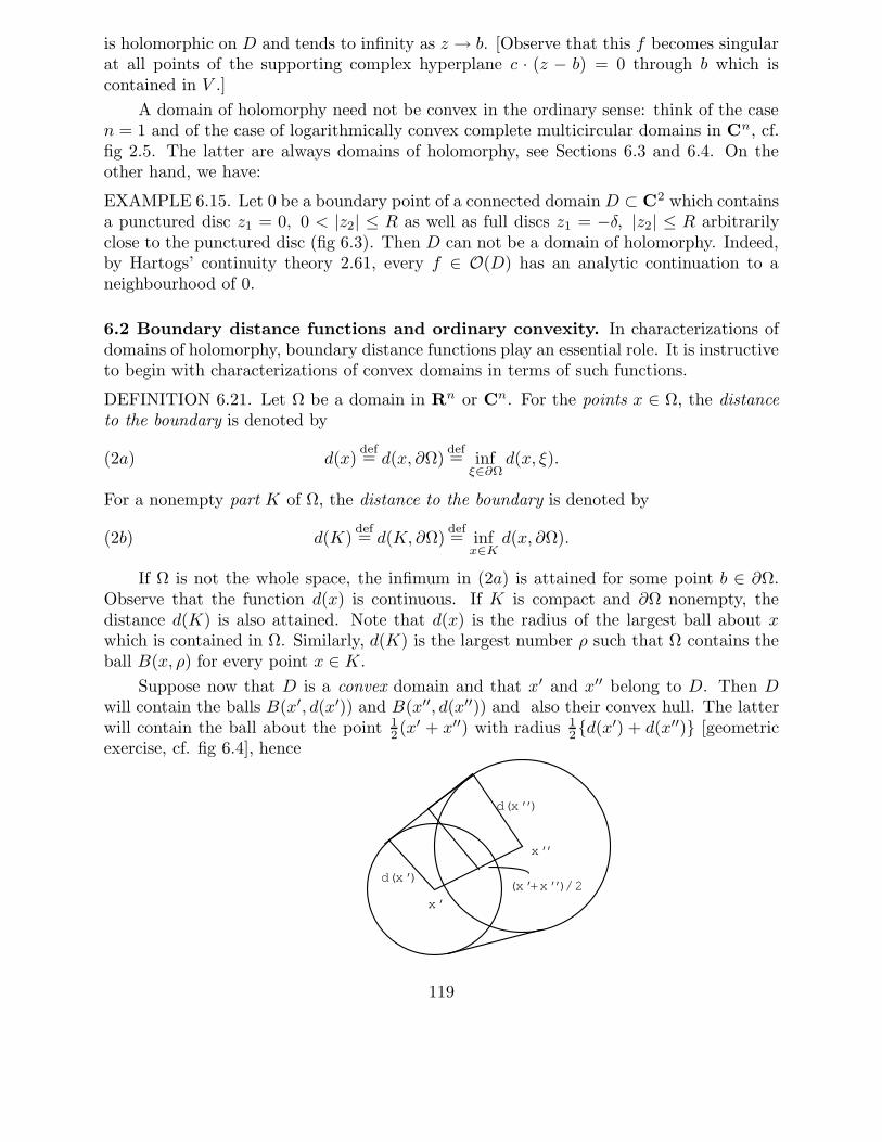
is holomorphic on D and tends to infinity as z → b. [Observe that this f becomes singularat all points of the supporting complex hyperplane c · (z − b) = 0 through b which iscontained in V .]

A domain of holomorphy need not be convex in the ordinary sense: think of the casen = 1 and of the case of logarithmically convex complete multicircular domains in Cn, cf.fig 2.5. The latter are always domains of holomorphy, see Sections 6.3 and 6.4. On theother hand, we have:

EXAMPLE 6.15. Let 0 be a boundary point of a connected domain D ⊂ C2 which containsa punctured disc z1 = 0, 0 < |z2| ≤ R as well as full discs z1 = −δ, |z2| ≤ R arbitrarilyclose to the punctured disc (fig 6.3). Then D can not be a domain of holomorphy. Indeed,by Hartogs’ continuity theory 2.61, every f ∈ O(D) has an analytic continuation to aneighbourhood of 0.

6.2 Boundary distance functions and ordinary convexity. In characterizations ofdomains of holomorphy, boundary distance functions play an essential role. It is instructiveto begin with characterizations of convex domains in terms of such functions.

DEFINITION 6.21. Let Ω be a domain in Rn or Cn. For the points x ∈ Ω, the distanceto the boundary is denoted by

(2a) d(x)def= d(x, ∂Ω)

def= inf

ξ∈∂Ωd(x, ξ).

For a nonempty part K of Ω, the distance to the boundary is denoted by

(2b) d(K)def= d(K, ∂Ω)

def= inf

x∈Kd(x, ∂Ω).

If Ω is not the whole space, the infimum in (2a) is attained for some point b ∈ ∂Ω.Observe that the function d(x) is continuous. If K is compact and ∂Ω nonempty, thedistance d(K) is also attained. Note that d(x) is the radius of the largest ball about xwhich is contained in Ω. Similarly, d(K) is the largest number ρ such that Ω contains theball B(x, ρ) for every point x ∈ K.

Suppose now that D is a convex domain and that x′ and x′′ belong to D. Then Dwill contain the balls B(x′, d(x′)) and B(x′′, d(x′′)) and also their convex hull. The latterwill contain the ball about the point 1

2 (x′ + x′′) with radius 12d(x′) + d(x′′) [geometric

exercise, cf. fig 6.4], hence

x’

x’’

d(x’’)

d(x’)(x’+x’’)/2

fig 6.4

119

(2c) d( 12(x′ + x′′)) ≥ 1

2d(x′) + d(x′′) ≥√

d(x′)d(x′′).

It follows that the function

(2d) v(x)def= log 1/d(x) = − log d(x)

satisfies the following mean value inequality on the line segments in D :

(2e) v( 12(x′ + x′′)) ≤ 1

2v(x′) + v(x′′);

the value of v at the midpoint of a line segment is majorized by the mean of the values atthe end points.

A continuous function v on a domain D with property (2e) is a so-called convexfunction: the graph on line segments in D lies below [never comes above] the chords. Informula:

(2f) v((1− λ)x′ + λx′′) ≤ (1− λ)v(x′) + λv(x′′), ∀λ ∈ [0, 1], ∀[x′, x′′] ⊂ D.

For dyadic fractions λ = p/2k this follows from the mean value inequality by repeatedbisection of segments; for other λ one uses continuity. [For our special function v one canalso derive (2f) from fig 6.4 and properties of the logarithm, cf. Exercise 6.6.] We havethus proved:

Proposition 6.22. On a convex domain D, the function v = log 1/d is convex.

Conversely, one can show that convexity of the function v = log 1/d on a connecteddomain D implies convexity of the domain, cf. Exercises 6.7, 6.8.

We still remark that on any bounded domain Ω, the function log 1/d is a so-calledexhaustion function:

DEFINITION 6.23. Let Ω in Rn or Cn be open. A continuous real function α on Ω iscalled exhaustion function for Ω if the open sets

(2g) Ωt = z ∈ Ω : α(z) < t, t ∈ R

have compact closure [are “relatively compact”] in Ω.

Observe that the sets Ωt jointly exhaust Ω : ∪Ωt = Ω. For Ω equal to the whole spaceRn, the function |x|2 is a convex exhaustion function:

∣

∣

12(x′ + x′′)

∣

∣

2 ≤ 12 (|x′|2 + |x′′|2).

Every convex domain has a convex exhaustion function, and every connected domain witha convex exhaustion function is convex, cf. Exercises 6.7, 6.8.

120

another characteristic property of convex domains. Let D be a connecteddomain in Rn or Cn and let K be a nonempty compact subset of D. To start out we againsuppose that D is convex. Then the convex hull CH(K) will also be a compact subset ofD. We will in fact show that it has the same boundary distance as K itself:

(2h) d(CH(K)) = d(K).

Indeed, as we know [Section 2.2], any point x ∈ CH(K) can be represented as a finite sum

x =

m∑

1

λjsj with sj ∈ K, λj ≥ 0 and∑

λj = 1.

Now by (2f) or fig 6.4, all points y = (1− λ)s1 + λs2, 0 ≤ λ ≤ 1 of a segment [s1, s2] ⊂ Dsatisfy the inequality

d(y) ≥ mind(s1), d(s2).

Hence for our point x, using induction,

d(x) ≥ mind(s1), . . . , d(sm) ≥ d(K).

Thus d(CH(K)) ≥ d(K) and (2h) follows.Conversely, let D be any domain with property (2h), or simply a domain such that

CH(K) is a compact subset of it whenever K is one. Then D must be convex. Indeed, forany two points x′, x′′ ∈ D one may take K = x′, x′′. Then CH(K) is the line segment[x′, x′′] and by the hypothesis it belongs to D.

We summarize as follows:

Proposition 6.24. The following conditions on a connected domain D in Rn or Cn areequivalent:(i) D is convex;

(ii) d(CH(K)) = d(K) for every compact subset K of D;(iii) CH(K) is a compact subset of D for every compact K ⊂ D.

In Section 6.4 we will prove an analogous characterization for domains of holomorphyΩ in Cn. It will involve the so-called holomorphically convex hull of K in Ω.

6.3 Holomorphic convexity. As an introduction we characterize the ordinary convexhull CH(K) for compact K ⊂ Cn with the aid of holomorphic functions. One may describeCH(K) as the intersection of all closed half-spaces containing K [cf. Section 2.2]. It is ofcourse sufficient to take the minimal half-spaces containing K — those that are boundedby a supporting hyperplane. In Cn those half-spaces are given by the inequalities

(3a) Re c · z ≤ Re c · b = supζ∈K

Re c · ζ, c ∈ Cn − 0,

121

where b is an appropriate boundary point of K associated with the direction c (cf. 6.14).Thus the convex hull of K ⊂ Cn may be described as follows:

(3b)

CH(K) = z ∈ Cn : Re c · z ≤ supζ∈K

Re c · ζ, ∀c ∈ Cn

= z ∈ Cn : |ec·z| ≤ supζ∈K|ec·ζ |, ∀c ∈ Cn.

In the last line, CH(K) is described with the aid of the special class of entire functionsf(z) = exp(c · z), c ∈ Cn. If one uses a larger class of holomorphic functions, one obtainsa smaller [no larger] hull for K, depending on the class [see for example Exercise 6.16].In the following definition, the class of admissible holomorphic functions and the resultinghull are determined by a domain Ω containing K.

DEFINITION 6.31. Let Ω ⊂ Cn be a domain K ⊂ Ω nonempty and compact (or at leastbounded). The O(Ω)-convex hull KΩ, or holomorphically convex hull of K relativeto Ω, is the set

(3c) KΩdef= z ∈ Ω : |f(z)| ≤ ‖f‖K = sup

ζ∈K|f(ζ)|, ∀f ∈ O(Ω).

Before turning to examples we give another definition.

DEFINITION 6.32. Let Ω be a domain in Cn and let ϕ be a continuous map from theclosed unit disc ∆1(0, 1) ⊂ C to Ω which is holomorphic on the open disc ∆1 = ∆1(0, 1).Then ϕ, or rather

∆ = ∆ϕdef= ϕ(∆1)

is called a (closed) analytic disc in Ω. The image Γ = Γϕ = ϕ(C) of the boundary C = ∂∆1

will be called the edge of the analytic disc:

edge ∆ϕdef= Γϕ = ϕ(∂∆1).

EXAMPLES 6.33. (i) Let ∆ = ∆1(a, r) be a closed disc in Ω ⊂ C and let Γ = ∂∆. Thenby the maximum principle

|f(w) ≤ ‖f‖Γ ∀w ∈ ∆, ∀f ∈ O(Ω),

hence the holomorphically convex hull ΓΩ contains the disc ∆. The function f(w) = w−ashows that ΓΩ = ∆. Compare Exercise 6.12, however.

(ii) More generally, let Ω be a domain in Cn and let ∆ϕ be an analytic disc in Ω.Now let f be in O(Ω). Applying the maximum principle to the composition f ϕ on ∆1,we find that the hull ΓΩ of the edge Γ must contain the whole analytic disc ∆ϕ :

|f(z)| = |f ϕ(w)| ≤ ‖f ϕ‖C(0,1) = ‖f‖Γ, ∀z = ϕ(w) ∈ ∆ϕ.

122

0 1 3

D

2

Γ

|z2|

|z1|

fig 6.5

(iii) Let D ⊂ C2 be the multicircular domain (fig 6.5)

D = |z1| < 1, |z2| < 3 ∪ |z1| < 3, 1 < |z2| < 3,

Γ the circle z1 = 2, |z2| = 2 in D. Every function f in O(D) has an analytic continuationto the equiradial bidisc ∆2(0, 3), cf. Section 2.5. The holomorphically convex hull of Γrelative to the bidisc will be the disc z1 = 2, |z2| ≤ 2 [why not more?]. Hence ΓD is thepart of that disc which belongs to D :

ΓD = z ∈ C2 : z1 = 2, 1 < |z2| ≤ 2.

PROPERTIES 6.34. (a) KΩ is closed relative to Ω since we are dealing with continuousfunctions f in Definition 6.31. Also, KΩ is a bounded set even if Ω is not, since by (3b)

KΩ ⊂ CH(K) ⊂ B(0, R) whenever K ⊂ B(0, R).

However, KΩ need not be compact, cf. Example (iii) above. We will see in Section 6.4that noncompactness of KΩ can occur only if Ω fails to be a domain of holomorphy.

(b) for any point z0 ∈ Ω−KΩ and arbitrary constants A ∈ C, ε > 0 there is a functiong in O(Ω) such that

(3d) g(z0) = A, ‖g‖K < ε.

Indeed, there must be a function f in O(Ω) for which |f(z0)| > ‖f‖K . Now takeg = Afp/f(z0)p with sufficiently large p.

123

DEFINITION 6.35. A domain Ω ⊂ Cn is called holomorphically convex if the O(Ω)-convex hull KΩ is compact for every compact subset K of Ω.

Holomorphic convexity will provide a characterization for domains of holomorphy[Section 6.4].

EXAMPLES 6.36. (i) Every domain Ω ⊂ C is holomorphically convex. Indeed, for anycompact K ⊂ Ω, the bounded, relatively closed subset KΩ of Ω must be closed in C [andhence compact]. Otherwise KΩ would have a limit point b in ∂Ω. The function 1/(z − b)which is bounded on K would then fail to be bounded on KΩ.

(ii) Every logarithmically convex complete multicircular domain D ⊂ Cn is holomor-phically convex. We sketch the proof, taking n = 2 for convenience. Let K ⊂ D becompact. Enlarging K inside D, we may assume that K is the union of finitely manyclosed polydiscs. Now let b be any point in ∂D. In the plane of |z1|, |z2|, there will be acurve α1 log |z1|+ α2 log |z2| = c with αj ≥ 0 that separates the point (|b1|, |b2|) from thetrace of K. To verify this, one may go to the plane of log |z1|, log |z2| in which log trD isa convex domain. It may finally be assumed that the numbers αj are rational or, removingdenominators, that they are nonnegative integers. The monomial f(z) = zα1

1 zα2

2 will then

satisfy the inequality |f(b)| > ‖f‖K , hence b can not be a limit point of KD.

6.4 The Cartan-Thullen characterizations of domains of holomorphy. We beginwith an important auxiliary result on simultaneous analytic continuation (see also Exercise6.26 !):

Proposition 6.41. Let K be a compact subset of Ω ⊂ Cn, let a be a point of the O(Ω)-convex hull KΩ and let f be any holomorphic function on Ω. Then the power series for fwith center a converges (at least) throughout the ball B(a, d(K)) and uniformly on everycompact subset of that ball. More generally, if g is any function in O(Ω) which is majorizedby the boundary distance function d on K:

(4a) |g(ζ)| ≤ d(ζ), ∀ζ ∈ K,

then the power series for f around a converges throughout the ball B(a, |g(a)|).

PROOF. The first result is the special case g ≡ d(K) of the second. We will prove thefirst result and then indicate what has to be done to obtain the more general one.

Observe that the unit ball B(0, 1) is the union of the maximal polydiscs ∆(0, r) whichit contains, that is, the polydiscs for which r = (r1, . . . , rn) has length 1. Taking 0 < λ <d(K), let Kλ be the λ-neighbourhood of K, that is, the set of all points in Cn at a distance< λ from K. The closure Kλ will be a compact subset of Ω; note that we may representit in the form

Kλ =⋃

ζ∈K

B(ζ, λ) =⋃

ζ∈K, |r|=1

∆(ζ, λr).

124

Naturally, Mλ = sup |f | on Kλ will be finite. Applying the Cauchy inequalities 1.65 to fon ∆(ζ, λr), ζ ∈ K, |r| = 1, we obtain

(4b)∣

∣Dαf(ζ)∣

∣ ≤ Mλα!

(λr)α=

Mλα!

(λr1)α1 . . . (λrn)αn, ∀α ≥ 0.

For given α, the right-hand side furnishes a uniform bound for the modulus of the holo-morphic function Dαf throughout K, hence a bound for ‖Dαf‖K . Since a belongs to KΩ,the same bound must be valid for |Dαf(a)|. [Use (3c) for Dαf .] It follows that the powerseries for f with center a,

(4c)∑

α≥0

Dαf(a)

α!(z − a)α,

will converge at every point z with |zj − aj | < λrj , j = 1, . . . , n. In other words, itconverges throughout the polydisc ∆(a, λr). This holds for all λ < d(K) and all r with|r| = 1, hence the series converges throughout the union B(a, d(K)) of those polydiscs,and it converges uniformly on every compact subset of that ball. [Cf. Theorem 2.42.]

For the second result one takes 0 < λ < 1 and introduces the set

K∗λ =

⋃

ζ∈K

B(ζ, λ|g(ζ)|).

This too is a compact subset of Ω [use (4a) and the continuity of g]. Instead of (4b) onenow obtains |Dαf(ζ)| ≤M∗

λα!/(λ|g(ζ)|r)α or

(4d)∣

∣Dαf(ζ) · g(ζ)|α|∣

∣ ≤ M∗λα!

(λr)α, ∀α ≥ 0, |r| = 1.

These inequalities hold throughout K [also where g(ζ) = 0]; they will extend to the pointa ∈ KΩ. Via the convergence of the series (4c) throughout the polydiscs ∆(a, λ|g(a)|r)with λ < 1 and |r| = 1, one obtains its convergence on the union B(a, |g(a)|).

One more definition and we will be ready for the main result.

DEFINITION 6.42. Ω ⊂ Cn is called the (maximal) domain of existence for the functionf ∈ O(Ω) if for every (small) connected domain U that intersects the boundary of Ω and forevery component Ω1 of U ∩Ω, it is impossible to continue the restriction f |Ω1

analyticallyto U , cf. fig 6.1.

Theorem 6.43. (cartan-thullen). The following conditions on a domain Ω ⊂ Cn areequivalent:

(i) Ω is a domain of holomorphy;(ii-a) For every compact subset K ⊂ Ω, the holomorphically convex hull KΩ has the

same distance to the boundary ∂Ω as K:

d(KΩ) = d(K);

125

(ii-b) All holomorphic functions g on Ω which are majorized by the function d on Kare majorized by d on KΩ :

(4e) |g(ζ)| ≤ d(ζ), ∀ζ ∈ K =⇒ |g(z)| ≤ d(z), ∀z ∈ KΩ;

(iii) Ω is holomorphically convex, that is, KΩ is a compact subset of Ω whenever K is;(iv) Ω is the maximal domain of existence for some function f ∈ O(Ω).

PROOF. For the proof we may assume that Ω is connected: if Ω is a domain of holomorphy,so are all its components and conversely. We may also assume Ω 6= Cn and will write Kfor KΩ.

(i) ⇒ (ii-a). Since K ⊂ K one has d(K) ≤ d(K). For the other direction, chooseany point a in K. For any function f in O(Ω), the power series with center a converges(at least) throughout the ball B = B(a, d(K)) [Proposition 6.41]. The sum of the seriesfurnishes a direct analytic continuation of f [from the component of Ω ∩ B that containsa] to B and this holds for all f in O(Ω). However, by the hypothesis Ω is a domain ofholomorphy, hence B must belong to Ω or we would have a contradiction. It follows thatd(a) ≥ d(K) and, by varying a. that d(K) ≥ d(K).

(i) ⇒ (ii-b). This implication also follows from Proposition 6.41. If (4a) holds forg ∈ O(Ω), the power series for any f ∈ O(Ω) with center a ∈ K will define a holomorphicextension of f to B(a, |g(a)|), hence such a ball must belong to Ω. Thus d(a) ≥ |g(a)| and(4e) follows.

(ii-a) or (ii-b) ⇒ (iii). Let K ⊂ Ω be compact. Because (ii-b) implies (ii-a) [takeg ≡ d(K)] we may assume (ii-a). We know that K ⊂ Ω is bounded and closed relative toΩ [Properties 6.34]. Since by the hypothesis K has positive distance to ∂Ω, it follows thatK is compact.

(iii) ⇒ (iv). We will construct a function f in O(Ω) that has zeros of arbitrarily highorder associated to any boundary approach.

Let aν be a sequence of points that lies dense in Ω and let Bν denote the maximalball in Ω with center aν . Let Eν be the “standard exhaustion” of Ω by the increasingsequence of compact subsets

Eν = z ∈ Ω : |z| ≤ ν, d(z, ∂Ω) ≥ 1/ν, ν = 1, 2, . . . ;

∪Eν = Ω. By changing scale if necessary we may assume that E1 is nonempty. By (iii)the subsets Eν ⊂ Ω are also compact. Since Bν contains points arbitrarily close to ∂Ω, wecan choose points

ζν in Bν − Eν , ν = 1, 2, . . . .

We next choose functions gν in O(Ω) such that

gν(ζν) = 1, ‖gν‖Eν< 2−ν , ν = 1, 2, . . .

[cf. formula (3d)]. Our function f is defined by

(4f) f(z) =

∞∏

ν=1

1− gν(z)ν , z ∈ Ω;

126

we will carefully discuss its properties. For the benefit of readers who are not thoroughlyfamiliar with infinite products, we base our discussion on infinite series.

We begin by showing that the infinite product in (4f) is uniformly convergent onevery set Eµ. Let z be any point in Eµ. Then for ν ≥ µ

|gν(z)| ≤ ‖gν‖Eµ≤ ‖gν‖Eν

< 2−ν .

Using the power series −∑ws/s for the principal value of log(1 − w) on the unit disc|w| < 1, it follows that

ν|p.v. log1− gν(z)| ≤ ν|gν(z) + 12gν(z)2 + . . . | < 2ν2−ν .

Thus the series∑

ν≥µ

ν p.v. log1− gν(z)

is uniformly convergent on Eµ; the sum function is holomorphic on the interior E0µ. Ex-

ponentiating, we find that the product

∏

ν≥µ

1− gν(z)ν

is also uniformly convergent on Eµ; the product function is zero free on Eµ and holomorphicon E0

µ.Multiplying by the first µ−1 factors, the conclusion is that the whole product in (4f)

converges uniformly on Eµ. The product defines f as a holomorphic function on E0µ and

hence on Ω. Since f is zero free on E1 it does not vanish identically; on Eµ it vanishesprecisely where one of the first µ− 1 factors of the product is equal to zero. At the pointz = ζν ∈ Bν the factor 1− gν(z)ν vanishes of order ≥ ν, hence the same holds for f.

We will show that f can not be continued analytically across ∂Ω. Suppose on thecontrary that f has a direct analytic continuation F to a connected domain U intersecting∂Ω if one starts from the component Ω1 of U ∩ Ω. Now choose a point b in ∂Ω1 ∩ Uand select a subsequence a′k = aνk

of aν which lies in Ω1 and converges to b. Theassociated balls B′

k = Bνkmust also tend to b, hence for large k they lie in Ω1 and by

omitting a few, we may assume that they all do. At z = ζ ′k = ζνk∈ B′

k our function fvanishes of order ≥ νk ≥ k and the same must then hold for F . Thus

DαF (ζ ′k) = 0 for all α,s with |α| < k.

Since ζ ′k → b it follows by continuity that DαF (b) = 0 for every multi-index α, henceF ≡ 0. By the uniqueness theorem this would imply f ≡ 0, but that is a contradiction.

(iv) ⇒ (i): clear.

REMARK 6.44. One can show that a result like 6.43(ii-a) is also valid for other distancelike functions, e.g., as introduced in exercise 6.27. , cf. [Pflug].

127

6.5 Domains of holomorphy are pseudoconvex. On a convex domain Ω the functionv = log 1/d is convex: it satisfies the linear mean value inequality (2e), or with differentletters,

(5a) v(a) ≤ 12v(a− ξ) + v(a+ ξ)

for every straight line segment [a− ξ, a+ ξ] in Ω. Pseudoconvexity of a domain Ω in Cn

may be defined in terms of a weaker mean value inequality for the function v = log 1/d.In the case n = 1 this will be the inequality that characterizes subharmonic functions:

DEFINITION 6.51. A continuous subharmonic function v on Ω ⊂ C is a continuousreal valued function that satisfies for every point a ∈ Ω and all sufficiently small vectorsζ ∈ C− 0, v the circular mean value inequality:

(5b) v(a) ≤ v(a; ζ)def=

1

2π

∫ π

−π

v(a+ eitζ)dt, 0 < |ζ| < ra.

In the present case of C one may write ζ = reiϕ and thus v(a; ζ) = v(a; r), the mean valueof v over the circle C(a, r). For subharmonic v as defined here, the mean value inequality(5b) will automatically hold for every ζ with 0 < |ζ| < d(a) [one may take ra = d(a),Section 8.2].

In the case of Cn, the mean value inequality relative to circles in complex lines leadsto the class of plurisubharmonic functions:

DEFINITION 6.52. A continuous plurisubharmonic (psh) function v on Ω ⊂ Cn is acontinuous real function with the property that its restrictions to the intersections of Ωwith complex lines are subharmonic. Equivalently, it is required that for every point a ∈ Ωand every vector ζ ∈ Cn−0, the function v(a+wζ), w ∈ C satisfy circular mean valueinequalities at the point w = 0. The condition may also be expressed by formula (5b), butnow for vectors ζ ∈ Cn.

It may be deduced from (5a) [by letting ξ run over a semicircle] that convex functionson Ω ⊂ Cn are plurisubharmonic. An important example is given by the function |z|2.Observe also that the sum of two psh functions is again psh

More general [not necessarily continuous] subharmonic and plurisubharmonic func-tions will be studied in Chapter 8. The following lemma is needed to prove circular meanvalue inequalities for continuous functions.

Lemma 6.53. Let f be a continuous real functions on the closed unit disc ∆1(0, 1) ⊂ Cwith the following special property:

Π For every polynomial p(w) such that Re p(w) ≥ f(w) on the circumference C(0, 1),one also has Re p(0) ≥ f(0). Then f satisfies the mean value inequality at 0 relativeto the unit circle:

f(0) ≤ f(0; 1) =1

2π

∫ π

−π

f(eit)dt.

128

PROOF. By Weierstrass’s theorem on trigonometric approximation, any 2π-periodic con-tinuous real function on R can be uniformly approximated, within any given distance ε,by real trigonometric polynomials

∑

k≥0

(ak cos kt+ bk sin kt) = Re∑

k≥0

(ak − ibk)eikt = Re p(eit).

Here p(w) stands for the polynomial∑

k≥0(ak − ibk)wk. For our given f , we now approx-

imate f(eit) + ε with error ≤ ε by Re p(eit) on R:

−ε ≤ f(eit) + ε− Re p(eit) ≤ ε.

Thenf(w) ≤ Re p(w) ≤ f(w) + 2ε on C(0, 1).

Hence by property (Π) of f ,

f(0) ≤ Re p(0) = a0 =1

2π

∫ π

−π

Re p(eit)dt

≤ 1

2π

∫ π

−π

f(eit)dt+ 2ε = f(0, 1) + 2ε.

The proof is completed by letting ε ↓ 0.

DEFINITION 6.54. A domain (open set) Ω in Cn is called pseudoconvex if the function

(5c) v(z) = log 1/d(z) = log 1/d(z, ∂Ω)

is plurisubharmonic on Ω.

There are also other definitions of pseudoconvexity possible, cf. Remark 6.57 andTheorem 9.34.

Theorem 6.55. Every domain of holomorphy in Cn is pseudoconvex.

PROOF. Let Ω ⊂ Cn be a domain of holomorphy. Choose any point a in Ω. We will showthat the function v = − log d satisfies the mean value inequality (5b) for every ζ ∈ Cn with0 < |ζ| < d(a). Fixing such a ζ, the flat analytic disc

∆ = z ∈ Cn : z = a+ wζ, |w| ≤ 1

will belong to Ω. We set

(5d) f(w) = v(a+ wζ) = − log d(a+ wζ), w ∈ ∆1(0, 1)

and get ready to apply Lemma 6.53 to this continuous real f .

129

Thus, let p(w) be any polynomial in w such that

(5e) Re p(w) ≥ f(w) = − log d(a+ wζ), ∀w ∈ C(0, 1).

In order to exploit the fact that Ω is a domain of holomorphy, we have to reformulate (5e)as an inequality for a holomorphic function on Ω. This is done by choosing a polynomialq(z) in z such that

(5f) q(a+ wζ) = p(w), ∀w ∈ C;

singling out a nonzero coordinate ζj of ζ, one may simply take q(z) = p(zj − aj)/ζj.Then for z = a+ wζ with w ∈ C(0, 1), (5e) gives

Re q(z) = Re p(w) ≥ − log d(z),

or equivalently,

(5g) |e−q(z)| ≤ d(z), ∀z ∈ Γ = edge ∆.

We know that ∆ ⊂ Ω belongs to the holomorphically convex hull of Γ relative to Ω, cf. 6.33.Now Ω is a domain of holomorphy, hence by the Cartan-Thullen theorem 6.43, inequality(5g) must also hold everywhere on ∆ ⊂ ΓΩ, cf. (4e). It will hold in particular for z = a,hence |e−q(a)| ≤ d(a) or

(5h) Re p(0) = Re q(a) ≥ − log d(a) = f(0).

Summing up, (5e) always implies (5h), so that f has property (∏

) of Lemma 6.53.Conclusion:

f(0) ≤ f(0; 1) or v(a) ≤ v(a; ζ).

We close with an important auxiliary result for the solution of the Levi problem inChapters 7, 11.

Proposition 6.56. Every pseudoconvex domain Ω has a plurisubharmonic exhaustionfunction: It is “psh exhaustible” The intersection Ω′ = Ω ∩ V of a psh exhaustibledomain Ω with a complex hyperplane V is also psh exhaustible.

PROOF. (i) If Ω = Cn, then the function |z|2 will do. For other pseudoconvex Ω, thefunction

α(z) = log1

d(z)+ |z|2, z ∈ Ω

will be a psh exhaustion function. Indeed, α is a sum of psh functions, hence psh, cf. Def-inition 6.54 and the lines following Definition 6.52. The term |z|2 ensures the compactnessof the subsets Ωt of Ω when Ω is unbounded, cf. Definition 6.23.

(ii) If α is any psh exhaustion function for Ω, then α′ = α |Ω′ will be a psh exhaustionfunction for Ω′ = Ω ∩ V . [Verify this.]

REMARK 6.57. Psh exhaustion functions are essential in the solution of the ∂ problem onpseudoconvex domains as presented in Chapter 11. For that reason, one sometimes definespseudoconvexity in terms of the existence of psh exhaustion functions. In fact, every pshexhaustible domain is also pseudoconvex in the sense of Definition 6.54 [cf. Section 9.3].

130

Exercises

6.1. Prove directly from the definition that Uj = z ∈ Cn : zj 6∈ 0 is a domain ofholomorphy. Prove also that Uj ∩ Uk is a domain of holomorphy.

6.2. Let Ω1 and Ω2 be domains of holomorphy in Cm and Cp, respectively. Prove that theproduct domain Ω = Ω1 × Ω2 is a domain of holomorphy in Cm+p.

6.3. (Analytic polyhedra) Let P be an analytic polyhedron in Cn, that is, P is compactand there exist a neighbourhood U of P and a finite number of holomorphic functionsf1, . . . , fk on U such that

P = z ∈ U : |fj(z)| < 1, j = 1, . . . , k.

Prove that P is a domain of holomorphy. [Examples: the polydisc ∆(a, r) withr <∞, the multicircular domain in C2 given by the set of inequalities |z1| < 2,|z2| < 2, |z1z2| < 1.]

6.4. Prove directly that the Reinhardt triangle

D = (z1, z2) ∈ C2 : 0 < |z1| < |z2| < 1

is a domain of holomorphy. [This is a logarithmically convex multicircular domainwhich, however, is not complete.]

D

|z2|

0 1

|z1|

fig 6.6

6.5. Prove that the closure D of the Reinhardt triangle can not be the intersection ofa family of domains of holomorphy. [Cf. Section 2.5.] Show in addition that everyholomorphic function on D which is bounded with all its derivatives of arbitrary order,extends to the polydisc ∆2(0, 1). [Cf. [Sibony] for related examples.]

6.6. Let D be convex and let x′, x′′ lie in D. Show that

d((1− λ)x′ + λx′′) ≥ (1− λ)d(x′) + λd(x′′), ∀λ ∈ [0, 1].

Now use the fact that the function log t is increasing and concave [the graph lies abovethe chords] to prove inequality (2f) for v = − log d.

131

6.7. Let D be a connected domain in Rn. A point b ∈ ∂D is called a boundary point ofnonconvexity for D if there is a straight line segment S throught b in D whose endpoints belong to D and which is the limit of a continuous family of line segmentsinside D. Suppose now that D is nonconvex. Prove that D has a boundary point ofnonconvexity. [There must be points x′, x′′ in D such that the segment [x′, x′′] doesnot belong to D. Connecting x′ to x′′ by a polygonal path in D, one may deduce thatD must contain segments [x0, x1] and [x0, x2] such that [x1, x2] does not belong to D.Now consider segments parallel to [x1, x2].]

6.8. (Continuation) Let D be a connected domain in Rn.(i) Suppose that the function v(x) = log 1/d(x) is convex on D.

Deduce that D is convex.(ii) Prove that D is convex if and only if it has a convex exhaustion function.

6.9. Let K ⊂ Rn be compact. Characterize the points x of the convex hull CH(K) bymeans of a family of inequalities involving real linear functions, cf. (3b).

6.10. Let K ⊂ Ω ⊂ Cn be compact, K = KΩ the holomorphically convex hull of K relativeto Ω. Prove that(i) (K)∧ = K;

(ii) if |zj | ≤ rj for all z ∈ K, then |zj | ≤ rj for all z ∈ K [hence K is bounded].

6.11. Suppose K ⊂ Zf ⊂ Ω, where Zf is the zero set of a function f ∈ O(Ω). Prove that

K ⊂ Zf .6.12. Let Ω ⊂ C be the annulus A(0, ρ, R) and let K be the circle C(0, r), where ρ < r < R.

Determine KΩ.

6.13. Let K ⊂ C be compact, C−K connected, a ∈ C−K. Prove that there is a simpleholomorphic function f on a neighbourhood Ω of K∪a with connected complementCe − Ω such that

|f(z)| ≤ 1 on K, |f(a)| > 1.

Next use Runge’s theorem 1.75 to show that there is a polynomial p(z) such that

|p(z)| ≤ 1 on K, |p(a)| > 1.

Finally, describe KC.

6.14. Let K be an arbitrary compact set in C [C−K need not be connected]. DescribeKC.

6.15. Let ∆ ⊂ Ω ⊂ Cn be a flat analytic disc, ∆ = z ∈ Cn : z = a+wζ, |w| ≤ 1, whereζ ∈ Cn − 0. Determine ΓΩ where Γ = edge ∆.

6.16. (Polynomially convex hull) For K ⊂ Cn compact, the polynomially convex hull K isdefined by

K = z ∈ Cn : |p(z)| ≤ ‖p‖K for all polynomials p.Prove:

132

(i) For any domain Ω containing K, KΩ ⊂ K;(ii) For any polydisc ∆ containing K, K∆ = K;

(iii) K = KCn ⊂ CH(K).

6.17. Let K ⊂ Ω ⊂ Cn be compact and let E be the set of those points z ∈ Ω, for whichthere is a constant Mz such that |f(z)| ≤ Mz‖f‖K for all f ∈ O(Ω). Prove thatE = KΩ.

6.18. Prove directly from Definition 6.35 that the following domains are holomorphicallyconvex:(i) Cn;

(ii) polydiscs in Cn;(iii) convex domains in Cn.

6.19. Prove that the intersection of two domains of holomorphy is again a domain of holo-morphy.

6.20. Let D1 be a connected domain of holomorphy in Cn and let D2 ⊂ Cn be analyticallyisomorphic to D1. Prove that D2 is also a domain of holomorphy.

6.21. Let Ω be a domain of holomorphy and let Ωε be the “ε-contraction” of Ω, that is,Ωε = z ∈ Ω : d(z) > ε. Prove that Ωε is also a domain of holomorphy. [ForK ⊂ Ωε, KΩε ⊂ KΩ.]

6.22. (Another characterization of domains of holomorphy) Prove that Ω ⊂ Cn is a domainof holomorphy if and only if the following condition is satisfied:

“For every boundary point b and every sequence of points ζν in Ω that con-verges to b, there is a holomorphic function f on Ω which is unbounded on thesequence ζν”.

[Let Ω be a domain of holomorphy and Kν an increasing exhaustion of Ω by compactsubsets, determined in such a way that Kµ+1−Kµ contains a point θµ of the sequenceζν. Define f =

∑

gµ, where the functions gµ ∈ O(Ω) are determined inductivelysuch that

|gµ(θµ)| > µ+

µ−1∑

ν−1

|gν(θµ)|, ‖gµ‖Kµ< 2−µ.

What can you say about |f(θµ)| ?]

6.23. Prove that Ω ⊂ Cn is a domain of holomorphy if and only if the following conditionis satisfied: For every compact K ⊂ Ω and every function f ∈ O(Ω),

supK

|f(z)|d(z)

= supK

|f(z)|d(z)

.

6.24. Let D be a connected domain of holomorphy, K ⊂ D compact. Prove that thereis an analytic polyhedron P such that K ⊂ P ⊂ D. Deduce that D is the limit ofan increasing sequence of analytic polyhedra Pν such that P ν ⊂ P 0

ν+1. [Assuming

133

K = K (as we may), associate certain functions to the boundary points of anε-neighbourhood of K.]

6.25. Use the mean value inequality (5a) for v = log 1/d on straight line segments to provethat every convex domain in Cn is pseudoconvex.

6.26. (Continuity principle for analytic discs, cf. Hartogs’ continuity theorem 2.61) Let Dbe a connected domain in Cn and let ∆ν, ν = 1, 2, . . . be a sequence of analyticdiscs in D which converges to a set E in Cn. Suppose that the edges Γν of the discs∆ν all belong to a compact subset K of D. Setting d(K) = ρ and taking any pointb ∈ E, prove that (suitable restrictions of) the functions f ∈ O(D) can be continuedanalytically to the ball B(b, ρ).

6.27 Let Ω be a domain of holomorphy. For a ∈ Cn \ 0 let

da(z) = da(z, ∂Ω) = supr : (z + λa) ∈ Ω ∀|λ| < r.

Let Γ be the edge of an analytic disc ∆ in Ω. Show that

da(Γ) = da(∆).

Next show that − log da(z) is psh on Ω and deduce a proof of step ii of Hartogs’singularity theorem (4.82), for all n ≥ 2.

6.28. (Prism Lemma). Let Hx be a domain in Rnx which contains two closed line segments

[x0, x1] and [x0, x2] that do not belong to a straight line and let f be holomorphicon Hx + iRn

y ⊂ Cn. Prove that f has an analytic continuation to a neighborhood ofTx+ iRn

y , where Tx is the closed triangular region with vertices x0, x1, x2. [ Take x0 =(0, 0, 0, . . . , 0), x1 = (1, 1, 0, . . . , 0), x2 = (−1, 1, 0, . . . , 0). By translation invariance, itis sufficient to prove that f has an analytic extension to a neighborhood of an arbitrarypoint a = (a1, a2, . . . , 0) ∈ T 0

x : |a1| < a2 < 1. Determine c and d such that a lies onthe parabola x2 = cx2

1 + d through x1 and x2 and then consider the family of analyticdiscs ∆λ = z ∈ T + iRn

y : z2 = cz21 + λ, z3 = · · · = zn = 0, 0 ≤ λ ≤ d = 1− c. The

boundaries Γλ belong to [x0, x1] ∩ [x0, x2]+ iRny . Verify that the projection of ∆λ

onto the z1-plane is given by the inequality |x1| ≤ c(x21 − y2

1) + λ.]

134

CHAPTER 7

The first Cousin problem, ∂ and the Levi problem

Towards the end of the nineteenth century, prominent mathematicians solved thefollowing problems:– Construct a meromorphic function f on C, or on a domain Ω ⊂ C, with poles atprescribed points and with a prescribed way of becoming infinite at the poles (results ofMittag-Leffler);– Construct a holomorphic function f on C, or on Ω ⊂ C, with zeros at prescribed pointsand with prescribed multiplicities of the zeros (results of Weierstrass).

The corresponding questions for Cn and for domains Ω ⊂ Cn were also raised and ledto the important first and second Cousin problem, respectively, seeSection 1.10. However, solutions for domains other than simple product domains did notappear until Oka started to make his major contributions around 1936. It seemed then thatthe Cousin problems are best considered on domains of holomorphy. Still, that was not thewhole story. Complete understanding came only with the application of sheaf cohomology[Cartan-Serre, early 1950’s, cf. Chapter 12 and the monograph [Grauert-Remmert]]. Morerecently, there has been increased emphasis on the role of the ∂ equation, especially afterHormander found a direct analytic solution for the general ∂ problem on pseudoconvexdomains [cf. Chapter 11].

Let us elaborate. The Cousin problems require a technique, whereby local solutionsmay be patched together to obtain a global solution. Techniques for the first Cousinproblem can be applied also to other problems, such as the holomorphic extension offunctions, defined and analytic on the intersection of a domain with a complex hyperplane,and the patching together of local solutions of the ∂ equation to a global solution. In thisChapter it will be shown that the reduced, so-called holomorphic Cousin-I problem isgenerally solvable on a domain Ω ⊂ Cn if and only if the “first order” ∂ equation ∂u = vis generally solvable on Ω. Indeed, smooth solutions of the holomorphic Cousin-I problemexist no matter what domain Ω one considers. Such smooth solutions can be modified toa holomorphic solution by the method of “subtraction of nonanalytic parts” if an only ifone can solve a related ∂ equation.

In Chapter 11 it will be shown analytically that every pseudoconvex domain is a ∂domain, that is, a domain on which all (first order) ∂ equations are solvable. For C2 itwill then follow that pseudoconvex domains, ∂ domains, Cousin-I domains (domains onwhich all first Cousin problems are solvable) and domains of holomorphy are all the same,cf. Sections 7.2, 7.7. The situation in Cn with n ≥ 3 is more complicated: see Sections7.2, 7.5 and the discussion of the Levi problem in Section 7.7; cf. also Chapter 12.

7.1 Meromorphic and holomorphic Cousin-I. A meromorphic function f on an openset Ω ⊂ C is a function which is holomorphic except for poles. The poles must be isolated:they can not have a limit point inside Ω, but there are no other restrictions. [A limit pointof poles inside Ω would be a singular point of f but not an isolated singularity, hencecertainly not a pole.] The classical existence theorem here is Mittag-Leffler’s: For any

135

open set Ω ⊂ C, any family of isolated points aλ ⊂ Ω and any corresponding family ofprincipal parts

fλ(z) =

mλ∑

s=1

cλs(z − aλ)−s,

there is a meromorphic function f on Ω which has principal part fλ at aλ for each λ butno poles besides the points aλ. That is, for each point aλ there is a small neighbourhoodUλ ⊂ Ω such that

(1a) f = fλ + hλ on Uλ, with hλ ∈ O(Uλ)

[hλ holomorphic on Uλ], while f is holomorphic on Ω − ∪λUλ. For a classical proof ofMittag-Leffler’s theorem, cf. Exercise 7.1, for a proof in the spirit of this Chapter, cf.Exercise 7.3.

Since analytic functions in Cn with n ≥ 2 have no isolated singularities [Chapters 2,3], meromorphy in Cn must be defined in a different way:

DEFINITION 7.11. A meromorphic function f on Ω ⊂ Cn [we write f ∈ M(Ω)] isa function which, in some (connected) neighbourhood Ua of each point a ∈ Ω, can berepresented as a quotient of holomorphic functions,

f = ga/ha on Ua, with ha 6≡ 0.

[The question of global quotient representations of meromorphic functions f will be con-sidered in Theorem 12.6x.]

Observe that a meromorphic function need not be a function in the strict sense thatit has a precise value everywhere: it is locally defined as an element of a quotient field. OnUa, the above f may be assigned a precise value (at least) wherever ha 6= 0 or ga 6= 0. Ameromorphic function is determined by its finite values,cf. Exercise 7.5.

Suppose now that for Ω ⊂ Cn one is given a covering by open subsets Uλ, where λruns over some index set Λ, and that on each set Uλ one is given a meromorphic functionfλ. One would like to know if there is a global meromorphic function f on Ω which oneach set Uλ becomes singular just like fλ, in other words, f should satisfy the conditions(1a). Of course, this question makes sense only if on each nonempty intersection

(1b) Uλµ = Uλ ∩ Uµ,

the functions fλ and fµ have the same singularities. One thus arrives at the followinginitial form of the first Cousin problem:

MEROMORPHIC FIRST COUSIN PROBLEM 7.12. Let Uλ, λ ∈ Λ be a coveringof Ω ⊂ Cn by open subsets and let the meromorphic functions fλ ∈ M(Uλ) satisfy thecompatibility conditions

(1c) fλ − fµ = hλµ on Uλµ with hλµ ∈ O(Uλµ), ∀λ, µ ∈ Λ.

136

The question is if there exists a meromorphic function f ∈ M(Ω) such that

(1d) f = fλ + hλ on Uλ with hλ ∈ O(Uλ), ∀λ ∈ Λ.

In looking for f , one may consider the holomorphic functions hλ as the unknowns.They must then be determined such that hµ − hλ = hλµ on Uλµ, cf. (1d) and (1c). By(1c), the functions hλµ will have to satisfy certain requirements:

hλµ = −hµλ on Uλµ, hλµ = hλν + hνµ on Uλµν = Uλ ∩ Uµ ∩ Uν ,etc. It turns out that the meromorphic Cousin problem can be reduced to a holomorphicproblem involving the known functions hλµ and the unknown functions hλ:

(HOLOMORPHIC) COUSIN-I PROBLEM or ADDITIVE COUSIN PROBLEM 7.13.Let Uλ, λ ∈ Λ be an open covering of Ω ⊂ Cn and let hλµ be a family of holomorphicfunctions on the (nonempty) intersections Uλµ that satisfy the compatibility conditions

(1e)

hλµ + hµλ = 0 on Uλµ, ∀λ, µ, ν ∈ Λ

hλµ + hµν + hνλ = 0 on Uλµν , ∀λ, µ, ν ∈ Λ.

The question is if there exist holomorphic functions hλ ∈ O(Uλ) such that

(1f) hλ − hµ = hλµ on Uλµ, ∀λ, µ ∈ Λ.

A family Uλ, fλ with functions fλ ∈ M(Uλ) that satisfy condition (1c) will be calleda set of meromorphic Cousin data on Ω; a family Uλ, hλµ with holomorphic functionshλµ ∈ O(Uλµ) that satisfy the conditions (1e) will be called a set of (holomorphic) Cousin-Idata on Ω. The above forms of the first Cousin problem are related in the following way:

Proposition 7.14. The meromorphic first Cousin problem on Ω with data Uλ, fλ hasa solution f (in the sense of (1d) if and only if there is a solution hλ to the holomorphicCousin-I problem on Ω with the data Uλ, hλµ derived from (1c). In particular, if allholomorphic Cousin-I problems on Ω are solvable, then so are all meromorphic first Cousinproblems on Ω.

PROOF. If the family hλ solves the holomorphic problem corresponding to the functionshλµ coming from (1c), then in view of (1f):

fλ + hλ = fµ + hµ on Uλµ, ∀λ, µ,hence one may define a global meromorphic function f on Ω by setting

fdef= fλ + hλ on Uλ, ∀λ.

Conversely, if f solves the meromorphic problem, then the family hλ given by (1d) solvesthe corresponding holomorphic problem.

We will see in the sequel that the theory for the holomorphic Cousin-I problem has anumber of applications besides the meromorphic problem.

137

DEFINITION 7.15. An open set Ω in Cn will be called a cousin-I domain if all holo-morphic first Cousin problems on Ω are solvable. By Proposition 7.14, all meromorphicfirst Cousin problems on such a domain are also solvable. If it is only known that allmeromorphic first Cousin problems on Ω are solvable, one may speak of a meromorphicCousin-I domain.

Are all meromorphic Cousin-I domains in Cn also holomorphic Cousin-I domains?The answer is known to be yes for n = 2, cf. Exercise 7.23. For n = 1 the answer is yesfor a trivial reason: by the theory below, all domains Ω in C are Cousin-I domains !

EXAMPLE 7.16. Let U1 and U2 be domains in C with nonempty intersection U12. Let h12

be any holomorphic function on U12. All boundary points of U12 may be bad singularitiesfor h12! Nevertheless, by the Cousin-I theory h12 can be represented as h2 − h1 withhj ∈ O(Uj). It does not seem easy to prove this directly! Cf. also Exercise 7.14.

Not all domains in C2 are Cousin-I domains:

EXAMPLE 7.17. Take Ω = C2 − 0,

Uj = z ∈ C2 : zj 6= 0, j = 1, 2; h12 = −h21 =1

z1z2, h11 = h22 = 0.

Question: Can one write h12 as h2 − h1 with hj ∈ O(Uj) ?Observe that U1 is a multicircular domain and that U1 = [C − 0] × C. Every

holomorphic function h1 on U1 is the sum of a (unique) absolutely convergent Laurentseries

∑

p,q

apqzp1zq2 ,

at least where z1z2 6= 0, cf. Section 2.7. Here apq = 0 whenever q < 0: indeed, for fixedz1 6= 0,

h1(z1, z2) =∑

q

(

∑

q

apqzp1

)

zq2

will be an entire function of z2, hence∑

p apqzp1 = 0 for every q < 0 and all z1 6= 0. Another

application of the uniqueness theorem for Laurent series in one variable completes the proofthat apq = 0 for all (p, q) with q < 0. Similarly every holomorphic function h2 on U2 is thesum of a Laurent series

∑

p,q

bpqzp1zq2

with bpq = 0 whenever p < 0. It follows in particular that

a−1,−1 = b−1,−1 = 0.

Thus a difference h2 − h1 with hj ∈ O(Uj) can not possibly be equal to the prescribedfunction h12 on U1 ∩ U2: the latter has Laurent series

∑

cpqzp1zq2 = z−1

1 z−12 hence 1 =

c−1,−1 6= b−1,−1 − a−1,−1. The present Cousin-I problem is not solvable.[A shorter but less informative proof is suggested in Exercise 7.6.]

138

The domain Ω = C2−0 is not a domain of holomorphy. [All holomorphic functionson Ω have an analytic continuation to C2, cf. Sections 2.6, 3.4.] This is not a coincidence:on a domain of holomorphy, all Cousin-I problems will be solvable [see Theorem 7.71].

7.2 Holomorphic extension of analytic functions defined on a hyperplane sec-tion. Certain holomorphic extensions may be obtained by solving Cousin problems:

Theorem 7.21. Let Ω ⊂ Cn be a [meromorphic] Cousin-I domain and let Ω′ be thenonempty intersection of Ω with some (affine) complex hyperplane V ⊂ Cn. Then everyholomorphic function h on Ω′ [interpreted as a subset of Cn−1] has a holomorphic extensiong to Ω.

PROOF. By suitable choice of coordinates it may be assumed that V is the hyperplanezn = 0, so that the (n−1)-tuples (z1, . . . , zn−1) = z′ can serve as coordinates in Ω′ = V ∩Ω. The given holomorphic function h(z′) on Ω′ can, of course, be extended to a holomorphicfunction [independent of zn] on the cylinder Ω′ ×C by setting h(z′, zn) = h(z′, 0) = h(z′).This observation solves the extension problem if Ω ⊂ Ω′ × C; the general case will behandled via a meromorphic Cousin problem.

We introduce a covering of Ω by a family of polydiscs contained in Ω; the polydiscswhich contain no point z with zn = 0 will be called Up’s, those containing some point ofV will be called Vq’s. Observe that if (z′, zn) ∈ Vq, then also(z′, 0) ∈ Vq ⊂ Ω, hence z′ ∈ Ω′ [see fig 7.1 and cf. Exercise 7.11.]

Vq

V

(z’,zn)

(z’,0)

fig 7.1One associates meromorphic Cousin data to the above covering that depend on the

given function h:

(2a) fp = 0 on each Up, fq(z′, zn) =

h(z′)

znon each Vq.

Since an intersection Up∩Vq contains no points z with zn = 0, the corresponding differencefp − fq = hpq is holomorphic on that intersection.

By the hypothesis, our meromorphic first Cousin problem is solvable. Let f be ameromorphic solution on Ω:

(2b) f =

fp + hp = hp on Up, hp ∈ O(Up), ∀p,

fq + hq = h(z′)/zn + hq on Vq, hq ∈ O(Vq), ∀q.

139

We now define

(2c) g = znf =

znhp on the polydisc Up, ∀p.

h(z′) + znhq at each point (z′, zn)

in the polydisc Vq, ∀q.

The function g is clearly holomorphic on Ω. It is equal to h on Ω′: the points of Ω withzn = 0 belong to polydiscs Vq, hence g(z′, 0) = h(z′).

Appropriate choice of h will provide the following important step in an inductivesolution of the Levi problem:

Theorem 7.22. Let Ω ⊂ Cn be a [meromorphic] Cousin-I domain. Suppose that the(nonempty) intersections of Ω with the complex hyperplanes in Cn are domains of holo-morphy when considered as subsets of Cn−1. Then Ω is a domain of holomorphy.

PROOF. Choose any (small) connected domain U that intersects the boundary of Ω andany component Ω0 of U ∩ Ω. We will construct a function g ∈ O(Ω) whose restrictiong | Ω0 can not be continued analytically to U [cf. Definition 6.11].

Take a point b ∈ U ∩ ∂Ω0 and a point a ∈ Ω0 such that the segment [a, b] belongs toU ; let c be the point of [a, b] ∩ ∂Ω0 closest to a [so that c ∈ ∂Ω; c may coincide with b].

U

Ω

Ω0

ac

b

fig 7.2We next select a complex hyperplane V which contains [a, b]. Since by hypothesis the

intersection Ω′ = V ∩ Ω is a domain of holomorphy, there is a holomorphic function h onΩ′ which becomes singular at c for approach along [a, c). [One may take a function h thatis unbounded on [a, c), cf. Exercise 6.22. For n = 2, cf. also Exercise 7.12.] Let g, finally,be a holomorphic extension of h to the Cousin-I domain Ω. Then the restriction of g to Ω0

has no analytic continuation to U : g must also become singular at c for approach along[a, c).

COROLLARY 7.23. Let Ω ⊂ Cn be a [meromorphic] Cousin-I domain and suppose thatthe same is true for the intersection of Ω with any affine complex subspace of Cn of anydimension k between 1 and n. Then Ω is a domain of holomorphy.

140

[Use induction on n; the intersections of Ω with complex lines are planar open sets,hence domains of holomorphy.]

Thus in C2, every [meromorphic] Cousin-I domain is a domain of holomorphy. Thisis no longer true in Cn with n ≥ 3. For example, it was shown by Cartan that Ω =Cn \Cm × (0, . . . , 0), n ≥ m+ 3 is a Cousin-I domain, cf. Exercise 7.10.

The method of proof of Theorem 7.22 gives another interesting criterion for a domainof holomorphy, see Exercise 7.24.

7.3 Refinement of coverings and partitions of unity. It is sometimes desirable torefine a given covering of Ω by open subsets. A covering Vj, j ∈ J of Ω is called arefinement of the covering Uλ, λ ∈ Λ if each set Vj is contained in some set Uλ. In orderto transform given Cousin data for the covering Uλ into Cousin data for the coveringVj, we introduce a refinement map, that is, a map σ : J → Λ such that

(3a) Vj ⊂ Uσ(j) for each j ∈ J.

[There may be several possible choices for Uσ(j): we make one for each j.]

REFINEMENT OF COUSIN DATA 7.31. Let Vj be an open covering of Ω,ϕjk ∈ O(Vjk). The data Vj , ϕjk are called a refinement of given Cousin-I data Uλ, hλµon Ω if the covering Vj is a refinement of Uλ, and if the functions ϕjk are obtainedfrom the functions hλµ via a refinement map σ, combined with restriction:

(3b) ϕjk = hσ(j)σ(k) |Vjk, ∀j, k ∈ J [Vjk ⊂ Uσ(j)σ(k)].

Let Uλ, hλµ be given holomorphic Cousin-I data for Ω and let Vj , ϕjk be a refine-ment. It is clear that the functions ϕjk (3b) will then satisfy the compatibility conditionsfor the covering Vj, cf. (1e), hence the data Vj , ϕjk are also Cousin-I data for Ω.

Proposition 7.32. The original Cousin-I problem Uλ, hλµ on Ω is (holomorphically)solvable if and only if the refined problem Vj, ϕjk is.

PROOF. Suppose we have a solution ϕj of the refined problem:

ϕk − ϕj = ϕjk = hσ(j)σ(k) on Vjk ⊂ Uσ(j)σ(k), ∀j, k ∈ J.

We want to construct appropriate functions hλ on the sets Uλ from the functions ϕj andhλµ. By the compatibility conditions (1e),

hσ(j)σ(k) + hσ(k)λ − hσ(h)λ = 0 on Uσ(j)σ(k) ∩ Uλ.

Combination of the two formulas shows that

ϕk + hσ(k)λ = ϕj + hσ(j)σ(k) + hσ(k)λ = ϕj + hσ(j)λ on Vjk ∩ Uλ.

141

For each λ ∈ Λ we may therefore define a function hλ in a consistent manner throughoutUλ by setting

(3c) hλdef= ϕj + hσ(j)λ on Uλ ∩ Vj , ∀j.

[Each point of Uλ belongs to some set Vj .] The (holomorphic) functions hλ, hµ will thensatisfy the relation

hµ − hλ = ϕj + hσ(j)µ − ϕj − hσ(j)λ = hλµ on Uλµ ∩ Vj

for each j, hence hµ − hλ = hλµ throughout Uλµ. Thus the family hλ will solve theoriginal Cousin-I problem.

The proof in the other direction is immediate: if hλ solves the original problem, thefamily obtained via the map σ, combined with restriction, will solve the refined problem.Indeed, if

ϕjdef= hσ(j) | Vj , ∀j ∈ J,

thenϕk − ϕj = hσ(k) − hσ(j) = hσ(j)σ(k) = ϕjk on Vjk.

SPECIAL OPEN COVERINGS 7.33. It is convenient to consider open coverings Vj ofΩ that have the following properties:

(3d)Vj is locally finite, that is, every compact subset of Ω

intersects only finitely many sets Vj ;

(3e) Vj has compact closure on Ω for each j.

Every special open covering Vj as above will be countably infinite: by (3e) it mustbe infinite, and by (3d) it is countable [cf. the proof below].

Lemma 7.34. Every open covering Uλ of Ω has a special refinement Vj – one thatsatisfies the conditions (3d, e).

PROOF. One may obtain such a refinement Vj of Uλ with the aid of the standardexhaustion of Ω by the compact subsets

Eν = z ∈ Ω : d(z, ∂Ω) ≥ 1/ν, |z| ≤ ν, ν = 1, 2, . . . .

Assuming E2 nonempty (as we may by changing the scale if necessary), one picks outfinitely many sets Uλ that jointly cover E2. The corresponding subsets Uλ∩E0

3 [E0=interiorof E] will provide the first sets Vj ; together, they cover E2. One next covers E3 − E0

2 byfinitely many sets Uλ and uses the corresponding subsets Uλ ∩ (E0

4 −E1) as the next setsVj ; jointly they cover E3 − E0

2 . In the next step one covers E4 − E03 by infinitely many

sets Uλ ∩ (E05 −E2), etc.

142

DEFINITION 7.35. A C∞ partition of unity on Ω subordinate to an open coveringUλ is a family of nonnegative C∞ functions βλ on Ω such that

∑

λ

βλ ≡ 1 on Ω and supp βλ ⊂ Uλ, ∀λ,

Here supp βλ is the support relative to Ω, that is, the smallest relatively closed subset ofΩ outside of which βλ is equal to 0.

Proposition 7.36. For every special covering Vj, j = 1, 2, ... of Ω satisfying the con-ditions (3d, e) there exists a C∞ partition of unity βj on Ω with βj ∈ C∞

0 (Vj), that is,supp βj is a compact subset of Vj , ∀j.

[Actually, there exist C∞ partitions of unity subordinate to any open covering Uλ;they may be obtained from those for special coverings by a simple device, cf. Exercise7.15.]

PROOF of the Proposition. We begin by constructing a family of nonnegative C∞ func-tions αj on Ω such that suppαj is a compact subset of Vj while α =

∑

j αj is a strictlypositive C∞ function on Ω. For appropriate εj > 0 with 4εj < diamVj , let Wj denote theset of all points in Vj whose distance to the boundary ∂Vj is greater than 2εj . It may andwill be assumed that the numbers εj have been chosen in such a way that the family Wjis still a covering of Ω. [One may first choose ε1 so small that the family W1, V2, V3, . . . isstill a covering, then choose ε2 so small that the family W1, W2, V3, . . . is still a covering,etc.]

For each j we now determine a nonnegative C∞ function αj on Ω which is strictlypositive on Wj and has compact support in Vj . [One may obtain αj by smoothing of thecharacteristic function of Wj through convolution with a nonnegative C∞ approximationto the identity ρε, ε = εj , whose support is the ball B(0, εj), cf. Section 3.3.] Observethat at any given point a ∈ Ω, at least one function αj will be > 0.

Since the covering Vj is locally finite, a closed ball B ⊂ Ω intersects only finitelymany sets Vj . Hence all but a finite number of functions αj are identically zero on B.It follows that the sum

∑

j αj defines a C∞ function α on B, and hence on Ω. By thepreceding, the sum function α will be > 0 throughout Ω.

The proof is completed by setting

βjdef= αj/α, ∀j.

7.4 Analysis of Cousin-I. Existence of smooth solutions. Suppose that the holo-morphic Cousin-I problem with data Uλ, hλµ on Ω has a holomorphic or smooth solutionhλ : hλ ∈ O(Uλ) or hλ ∈ C∞(Uλ) and hµ − hλ = hλµ on Uλµ. By refinement of thedata we may assume that the covering Uλ is locally finite and that we have been able toconstruct a C∞ partition of unity βλ on Ω, subordinate to the covering Uλ, cf. Section7.3.

143

We wish to analyze the function hλ and focus on a point a in Uλ. At such a point awe will have

(4a) hλ = hν + hνλ

for all indices ν such that a ∈ Uν . There are only finitely many such indices ν ! We multiply(4a) by βν and initially sum over precisely those indices ν for which a ∈ Uν (symbol

∑aν):

(4b)

(

∑

a

ν

βν

)

hλ =∑

a

ν

βνhν +∑

a

ν

βνhνλ (at the point a ∈ Uλ).

The value of the first sum will not change if we add the terms βν (equal to 0 !) whichcorrespond to the indices ν for which a 6∈ Uν . The sum over all ν’s is equal to 1 and thiswill hold at every point a ∈ Uλ:

(4c)∑

a

ν

βν =∑

ν∈Λ

βν = 1 (at a ∈ Uλ).

Products βνhν , whether they occur in the second sum (4b) or not, may be extendedto C∞ functions on Ω by defining βνhν = 0 on Ω− Uν ; indeed, βνhν = 0 outside a closedsubset of Uν anyway [closed relative to Ω]. The value of the second sum will not change ifwe add the terms zero corresponding to those ν’s, for which a 6∈ Uν :

(4d)∑

a

ν

βνhν =∑

ν∈Λ

βνhν (at a ∈ Uλ).

What can we say about the last sum (4d) on Uλ or elsewhere?On a closed ball B ⊂ Ω, only finitely many terms in the full sum

∑

βνhν are ever6= 0. Thus the full sum defines a C∞ function on B and hence on Ω:

(4e)∑

ν∈Λ

βνhνdef= u ∈ C∞(Ω).

B

Uλ

Uν∂Ω

supp βν

fig 7.3We now turn to the third sum in (4b), but there we will not go outside Uλ. Products

βνhνλ are defined only on Uλν . Such products can be extended to C∞ functions on Uλby setting them equal to 0 on Uλ − Uν : they vanish at the points of Uν close to Uλ − Uνanyway (fig 7.3). For indices ν such that Uν does not meet Uλ, we may simply define

144

βνhνλ as 0 throughout Uλ. We are again going to sum over all ν’s; at a ∈ Uλ this onlymeans that we add a number of zero terms to the original sum:

(4f)∑

a

ν

βνhνλ =∑

ν∈Λ

βνhνλ (at a ∈ Uλ).

What can we say about the last sum (4f)?On a closed ball B in Uλ, only finitely many terms in the full third sum

∑

βνhνλ areever 6= 0. Thus that sum defines a C∞ function on B and hence on Uλ:

(4g)∑

ν∈Λ

βνhνλdef= gλ ∈ C∞(Uλ).

Conclusion. Combining (4b− g), we see that at any point a ∈ Uλ:

hλ =

(

∑

a

ν

βν

)

hλ =∑

ν∈Λ

βνhν +∑

ν∈Λ

βνhνλ = u+ gλ.

Thus any holomorphic or C∞ soluation of the Cousin-I problem under consideration canbe represented in the form

(4h) hλ = u+ gλ on Uλ, ∀λ ∈ Λ,

where gλ ∈ C∞(Uλ) is given by (4g) and u ∈ C∞(Ω).Conversely, if we define functions hλ by (4h, g), they will always form at least a smooth

solution of the Cousin-I problem, no matter what open set Ω we have[see below]:

Theorem 7.41. Let Uλ, hλµ be any family of holomorphic Cousin-I data on Ω ⊂ Cn

which has been refined so that the covering Uλ is locally finite and there is a C∞ partitionof unity βλ on Ω subordinate to Uλ. Then the functions hλ defined by (4h, g), with anarbitrary C∞ function u on Ω, constitute a C∞ solution of the Cousin-I problem with thegiven data, and every C∞ solution of the problem is of that form.

PROOF. For functions hλ as in (4h, g) one has

(4i)

hµ − hλ = gµ − gλ =∑

ν∈Λ

(

βνhνµ − βνhνλ)

=

(

∑

ν∈Λ

βν

)

hλµ = hλµ on Uλµ, ∀λ, µ

because of the compatibility conditions (1e). Thus the functions hλ form a C∞ solutionof the Cousin-I problem, cf. (1f). That all C∞ solutions of the problem have the form(4h, g) follows from the earlier analysis.

145

Remark. That every holomorphic (or C∞!) Cousin-I problem for arbitrary open Ωis C∞ solvable can also be proved without refinement of the Cousin data – it suffices torefine the covering (if necessary), cf. Exercise 7.20.

7.5 Holomorphic solutions of Cousin-I via ∂. In Section 7.4 we have determined allC∞ solutions hλ of a given (suitably refined) holomorphic Cousin-I problem Uλ, hλµon an open set Ω. For a fixed C∞ partition of unity βλ subordinate to Uλ, they havethe form (4h):

hλ = u+ gλ on Uλ,

with gλ as in (4g) and an arbitrary C∞ function u on Ω.

QUESTION 7.51. Will there be a holomorphic solution among all the C∞ solutions hλ?We still have the function u at our disposal. For holomorphy of the smooth functions

hλ it is necessary and sufficient that

0 = ∂hλ = ∂u+ ∂gλ,

or

(5a) ∂u = −∂gλ on Uλ, ∀λ ∈ Λ.

The second members in (5a) can be used to define a global differential form v on Ω. Indeed,on an intersection Uλ ∩ Uµ, (4i) gives

(5b) ∂(gµ − gλ) = ∂(hµ − hλ) = ∂hλµ = 0

since hλµ ∈ O(Uλµ)! Thus we obtain a C∞ form v on Ω by setting

(5c) v =

n∑

j=1

vjdzjdef= −∂gλ = −

n∑

j=1

∂gλ∂zj

dzj on Uλ, ∀λ ∈ Λ.

The conditions (5a) on u can now be summarized by the single equation ∂u = v on Ω. Ifu satisfies this condition, then ∂hλ = 0, so that hλ is a holomorphic function for each λ.We have thus proved:

Proposition 7.52. The (suitably refined) holomorphic Cousin-I problem 7.13 on Ω has aholomorphic solution hλ if and only if the associated ∂ equation

(5d) ∂u = v on Ω,

with v given by (5c) and (4g), has a C∞ solution u on Ω.

Incidentally, it is clear from (5c) that v satisfies the integrability conditions ∂vk/∂zj =∂vj/∂zk. It will be convenient to introduce the following terminology:

146

DEFINITION 7.53. An open set Ω ⊂ Cn will be called a ∂ domain if all equations∂u = v on Ω, with (0, 1)-forms v of class C∞ that satisfy the integrability conditions, areC∞ solvable on Ω.

We will now prove the following important

Theorem 7.54. Every ∂ domain Ω in Cn is a Cousin-I domain 7.15, and conversely.

PROOF of the direct part. Let Ω be a ∂ domain. Then equation (5d) is C∞ solvable,hence by Proposition 7.52, every suitable refined (holomorphic) Cousin-I problem on Ω isholomorphically solvable. Proposition 7.32 on refinements now tells us that every Cousin-Iproblem on Ω is holomorphically solvable, hence Ω is a Cousin-I domain.

For the converse we need an auxiliary result on local solvability of the ∂ equation thatwill be proved in Section 7.6:

Proposition 7.55. Let v be a differential form∑n

1 vjdzj of class Cp

(1 ≤ p ≤ ∞) on the polydisc ∆(a, r) ⊂ Cn that satisfies the local integrability conditions∂vk/∂zj = ∂vj/∂zk. Then the equation ∂u = v has a Cp solution f = fs on every polydisc∆(a, s) with s < r. [If a certain differential dzk is absent from v (that is, if the coefficientvk is identically 0), one may take the corresponding number sk equal to rk. The solutionconstructed in Section 7.6 will actually be of class Cp+α, ∀α ∈ (0, 1).]

PROOF of Theorem 7.54, converse part. Let Ω be a Cousin-I domain and let v be anyC∞ differential form

∑n1 vjdzj on Ω that satisfies the integrability conditions. We cover

Ω by a family of “good” polydiscs Uλ, λ ∈ Λ, that is, polydiscs Uλ ⊂ Ω on which thereexists a C∞ solution fλ of the equation ∂u = v. Then on the intersections Uλµ:

∂(fλ − fµ) = v − v = 0,

hence

hλµdef= fλ − fµ ∈ O(Uλµ), ∀λ, µ.

Just as in Section 7.1 the differences hλµ will satisfy the compatibility conditions (1e),hence Uλ, hλµ is a family of holomorphic Cousin-I data for Ω. Since by the hypothesisall Cousin-I problems on Ω are (holomorphically) solvable, there is a family of functionshλ ∈ O(Uλ) such that

hλµ = hµ − hλon each nonempty intersection Uλµ. We now set

udef= fλ + hλ on Uλ, ∀λ.

This formula will furnish a global C∞ solution of the equation ∂u = v on Ω : fλ + hλ =fµ + hµ on Uλµ and

∂u = ∂fλ + ∂hλ = v + 0 = v on Uλ, ∀λ.

Conclusion: Ω is a ∂ domain.

147

7.6 Solution of ∂ on polydiscs. We first prove the important local solvability of the ∂equation asserted in Proposition 7.55. Next we will show that polydiscs (and in particularCn itself) are ∂ domains [“Dolbeault’s lemma”]. The latter result is not needed for thesequel, but we derive it to illustrate the approximation technique that may be used to provethe general solvability of ∂ on domains permitting appropriate polynomial approximation,cf. [Hormander 1], [Range].

PROOF of Proposition 7.55. It is convenient to take a = 0. For n = 1 the proof is verysimple. Just let ω be a C∞ cutoff function which is equal to 1 on ∆(0, s) and has supportin ∆(0, r). Then ωv can be considered as a Cp form on C which vanishes outside ∆(0, r).Hence the Cauchy-Green transform will provide a Cp solution of the equation ∂u = ωv onC and thus of the equation ∂u = v on ∆(0, s), cf. Theorem 3.13.

For n ≥ 2 we try to imitate the procedure used in Section 3.2 for the case where v hascompact support, but now there will be difficulties. These are due to the fact that we cannot multiply v by a nonzero C∞ function of compact support in ∆(0, r) and still preservethe integrability conditions. To get around that problem one may use induction on thenumber of differentials dzj that there actually present in v.

If v contains no differentials dzj at all, the equation is ∂u = 0 and every holomorphicfunction on ∆(0, r) is a Cp solution on the whole polydisc. Suppose now that preciselyq differentials dzj are present in v, among them dzn, and that the Proposition has beenestablished already for the case in which only q − 1 differentials dzj are present. As usualwe write z = (z′, zn) and we set

∆(0, r) = ∆n−1(0, r′)×∆1(0, rn) = ∆n−1 ×∆1(0, rn).

Choosing s as in the Proposition, so that in particular sn < rn, we let ω = ω(zn) bea cutoff function of class C∞

0 on ∆1(0, rn) ⊂ C which is equal to 1 on ∆1(0, sn). Definingωvj = 0 for |zn| ≥ rn, the product

ω(zn)v(z′, zn) = ωv1dz1 + . . .+ ωvndzn

represents a Cp form on ∆n−1 ×C which for fixed z′ ∈ ∆n−1 vanishes when|zn| ≥ Rn. Thus the Cauchy-Green transform of ωvn relative to zn provides a solution ϕto the equation ∂u/∂zn = ωvn on ∆n−1 ×C, cf. Theorem 3.13:

(6a) ϕ(z) = ϕ(z′, zn) = − 1

π

∫

C

ω(ζ)vn(z′, ζ)

ζ − zndξdη.

Observe that the function ϕ is of class Cp on ∆(0, r) and that the same holds for ∂ϕ/∂zn =ωvn.

We will determine the derivatives ∂ϕ/∂zj with j < n by differentiation under theintegral sign, noting that by the integrability conditions,

∂

∂zjω(ζ)vn(z′, ζ) = ω(ζ)

∂vj∂zn

(z′, ζ) =∂

∂ζω(ζ)vj(z

′, ζ) − vj(z′, ζ)∂ω

∂ζ.

148

Thus, referring to the representation for compactly supported functions of Corollary 3.12for the second step,

(6b)

∂ϕ

∂zj= − 1

π

∫

C

∂

∂ζω(ζ)vj(z

′, ζ) dξdηζ − zn

+1

π

∫

C

vj(z′, ζ)

ζ − zn∂ω

∂ζ(ζ)dξdη

= ω(zn)vj(z′, zn) + I(vj , ω), 1 ≤ j < n,

say. By inspection, the derivatives ∂ϕ/∂zj are of class Cp on ∆(0, r).We now introduce the differential form

(6c) w = v − ∂ϕ.

This new form is also of class Cp on ∆(0, r) and it satisfies the integrability conditions[forms ∂ϕ always do]. Moreover, if we restrict the form to∆n−1(0, r′)×∆1(0, sn), then it may be written as

w = w1dz1 + . . .+ wn−1dzn−1,

since ∂ϕ/∂zn = ωvn = vn on that polydisc. Finally, if dzk was absent from v, that is,vk = 0 and k > n, then by (6b) also ∂ϕ/∂zk = 0, so that wk = 0. Thus the new formw restricted to ∆n−1(0, r′)×∆1(0, sn) contains at most q − 1 differentials dzj . Hence bythe induction hypothesis, there is a Cp function ψ on the polydisc ∆n−1(0, s′)×∆1(0, sn)such that w = ∂ψ there. Conclusion:

(6d) v = ∂ϕ+ w = ∂(ϕ+ ψ) on ∆(0, s),

with ϕ+ ψ ∈ Cp.[Actually, the function ϕ in (6a) will be of class Cp+α, ∀α ∈ (0, 1), cf. Remarks 3.14

and Exercises 3.6, 3.9. Likewise, by induction, ψ ∈ Cp+α.]

Theorem 7.61. Let v =∑n

1 vjdzj be a differential form of class Cp (1 ≤ p ≤ ∞) onthe polydisc ∆(a, r) ⊂ Cn that satisfies the integrability conditions. Then the equation∂u = v has a Cp solution on ∆(a, r).

PROOF. We take a = 0 and introduce a strictly increasing sequence of polydiscs ∆k

[more precisely, ∆k ⊂ ∆k+1, k = 0, 1, 2, . . .] with center 0 and union ∆ = ∆(0, r). ByProposition 7.55 there are Cp functions fk on ∆k+1, k = 1, 2, . . . such that ∂fk = v on ∆k.Starting with such functions fk, we will inductively determine Cp functions uk, k = 1, 2, . . .on ∆ such that(i) supp uk ⊂ ∆k+1,(ii) ∂uk = v on ∆k,

(iii) |uk − uk−1| < 2−k on ∆k−2, k ≥ 2.

Let ωk be a sequence of Cp cutoff functions on Cn such that ωk = 1 on ∆k andsuppωk ⊂ ∆k+1. We define u1 = ω1f1 on ∆2, u1 = 0 on ∆ − ∆2 so that (i) and (ii)hold for k = 1. Now suppose that u1, . . . , uk have been determined in accordance with

149

conditions (i)-(iii). Since ∂(fk+1 − uk) = 0 on ∆k, the difference fk+1 − uk is holomorphicon that polydisc, hence equal to the sum of a power series around 0 which is uniformlyconvergent on ∆k−1. Thus one can find a polynomial pk such that

|fk+1 − uk − pk| < 2−k−1 on ∆k−1.

We may now define

uk+1 =

(fk+1 − pk)ωk+1 on ∆k+2,

0 on ∆−∆k+2

to obtain (i)-(iii) with k + 1 instead of k.By (iii) we may define a function u on ∆ by

u = u1 +

∞∑

2

(uk − uk−1);

the series will be uniformly convergent on every compact subset of ∆. Condition (ii) showsthat the terms uk−uk−1 with k > j are holomorphic on ∆j , hence ϕj =

∑

k>j(uk−uk−1)is holomorphic on ∆j . It follows that u = uj + ϕj is of class Cp on ∆j . Moreover, on ∆j

∂u = ∂uj + ∂ϕj = v + 0 = v.

Since these results hold for each j = 1, 2, . . . we are done.

The method of the previous theorem may be extended to show that products of planardomains are Cousin-I domains, cf. exercise 7.21. It seems difficult to determine if a givendomain is Cousin-I. The following theorem is sometimes useful.

Theorem 7.62. Let Uλ be some open cover of the domain Ω consisting of Cousin-Idomains. Ω is a Cousin-I domain if and only if for all Cousin-I data of the form Uλ, hλµthe Cousin-I problem is solvable.

PROOF. The only if part is clear. For the if part, suppose that we are given Cousin-Idata Vi, hij. Then Vi ∩ Uλ, hij are Cousin-I data on Uλ (here and in the sequel wedenote the restriction of a function to a smaller domain and the function itself with thesame symbol), hence there exist hλi ∈ O(Vi ∩ Uλ) with

hλi − hλj = hij on Uλ ∩ Vij .

On Uλµ ∩ Vij we find hλi − hλj = hij = hµi − hµj , therefore

hλi − hλj = hµi − hµj .

150

Thus hλi − hµi = hλj − hµj for all i, j on Uλµ and we may define hλµ ∈ O(Uλµ) by

hλµ = hλi − hµi on Vi ∩ Uλµ.

Are these consistent Cousin-I data? Yes: on Vi ∩ Uλµν we have

hλµ + hµν + hνλ = hλi − hµi + hµi − hνi + hνi − hλi = 0.

We can solve this Cousin-I problem with functions hλ ∈ O(Uλ). Now for all i we find onVi ∩ Uλµ

hλi − hµi = hλµ = hλ − hµ.Hence hλi −hλ = hµi −hµ on Vi∩Uλµ and we may conclude that hλi −hλ extends analyticallyto a function hi ∈ O(Vi). We claim that the hi provide a solution. Indeed, for all λ wehave on Uλ ∩ Vij

hi − hj = hλi − hλ − hλj + hλ = hij .

7.7 The Levi problem. It will be shown in Chapter 11 that every domain with aplurisubharmonic exhaustion function, or pseudoconvex domain, is a ∂ domain. Once thatfundamental result has been established, we can use Theorem 7.54 to conclude:

Theorem 7.71. Every pseudoconvex domain, and hence every domain of holomorphy, isa Cousin-I domain.

More important, the result of Chapter 11 will enable us to complete the solution ofthe Levi problem begun in Section 7.2:

Theorem 7.72. Every domain Ω in Cn with a plurisubharmonic exhaustion function, orpseudoconvex domain, is a domain of holomorphy.

PROOF. We use induction on the dimension. Suppose then that the result has beenestablished for dimension n − 1; dimension 1 is no problem since every domain in C is adomain of holomorphy. Now let Ω be a psh exhaustible domain in Cn, n ≥ 2. By thefundamental result to be proved in Chapter 11, Ω is a ∂ domain and hence a Cousin-I domain [Theorem 7.54]. On the other hand, the intersections Ω′ of Ω with (affine)complex hyperplanes are also psh exhaustible [Proposition 6.56]. Hence by the inductionhypothesis, they are domains of holomorphy when considered as open subsets of Cn−1.Thus by Theorem 7.22, Ω is a domain of holomorphy.

Remarks. For n = 2 the Levi problem was settled by Oka in 1942, while solutions forn ≥ 3 were obtained almost simultaneously by Bremermann, Norguet and Oka in the years1953-1954. After Dolbeault’s work on cohomology (1953-1956, cf. Chapter 12), it becameclear that a solution of the Levi problem could also be based on an analytic solution of ∂,but such a solution did not exist at the time!

Exercises

151

7.1. Prove the Mittag-Leffler theorem for Ω = C (Section 7.1) along the following classicallines:(i) Write down a rational function gk with the prescribed poles and principal parts

on the disc ∆(0, k), k = 1, 2, . . . ;(ii) Does the series g1 +

∑∞2 (gk−gk−1) converge on Ω? If not, how can it be modified

to ensure convergence, taking into account that gk − gk−1 is holomorphic on∆(0, k − 1)?

7.2. (Related treatment of ∂ on C) Let v be a Cp function on Ω = C, 1 ≤ p ≤ ∞.(i) Use a suitable Cauchy-Green transform (Section 3.1-(1f)) to obtain a Cp function

uk on C such that ∂uk/∂z = v on ∆(0, k);(ii) Determine a Cp solution u of the equation ∂u/∂z = v on Ω by using a suitable

modification of the series u1 +∑∞

2 (uk − uk−1).

7.3. Describe how one can solve the meromorphic first Cousin problem for C (Section 7.1)directly with the aid of a ∂ problem. [Using nonoverlapping discs ∆(aλ, rλ), let ωλ bea C∞ function on C with support in ∆(aλ, rλ) and equal to 1 on ∆(aλ,

12rλ). Then

u = f −∑ωλfλ must be a C∞ function on C. What conditions does ∂u/∂z have tosatisfy?]

7.4. Extend the constructions in Exercises 7.1, 7.2 to the case where Ω is:(i) the unit disc ∆(0, 1);

(ii) the annulus A(0; 1, 2).

7.5. Let U be a connected domain in Cn, g, h, g, h ∈ O(U), h 6≡ 0, h 6≡ 0. Suppose thatg/h = g/h outside Z(h) ∪ Z(h). Prove that gh = hg on U , so that [g/h] = [g/h] inthe quotient field for O(U).

7.6. Prove directly [without Laurent series] that the following meromorphic first Cousinproblem on Ω = C2 − 0 must be unsolvable:

f1 =1

z1z2on U1 = z1 6= 0, f2 = 0 on U2 = z2 6= 0.

[Cf. formula (2c).]

7.7. Let Ω1 be a Cousin-I domain in Cn and let Ω2 be analytically isomorphic to Ω1. Provethat Ω2 is also a Cousin-I domain.

7.8. Which holomorphic Cousin-I problems for Ω = C2 − 0 andUj = z ∈ C2 : zj 6= 0, j = 1, 2 are solvable and which are not?

7.9. Let Ω be the multicircular domain in Cn (n ≥ 2) given by

|z′| < 1, |zn| < 3 ∪ |z′| < 3, 1 < |zn| < 3, z′ = (z1, . . . , zn−1).

Prove that Ω is not a Cousin-I domain by indicating a holomorphic function on Ω ∩z1 = 2 that has no analytic extension to Ω.

7.10. Prove by computation that all Cousin-I problems for Ω = C3 − 0, Uj =z ∈ C3 : zj 6= 0, j = 1, 2, 3 are solvable:

152

(i) Show that it is sufficient to consider the case where

h23 = a zp1zq2zr3 , h31 = b zp1z

q2zr3, h12 = c zp1z

q2zr3 .

(ii) Suppose p < 0. Show that then a = 0, c = −b and (assuming b 6= 0)q ≥ 0, r ≥ 0. Solve.

(iii) Finally deal with the case p ≥ 0, q ≥ 0, r ≥ 0.(iv) Can you extend this to Cn \Cm, n−m ≥ 3?

7.11. Suppose that the polydisc ∆(a, r) in Cn meets the hyperplane zn = 0. What doesthis mean for an and rn? Prove that the intersection is precisely the projection of∆(a, r) onto the hyperplane.

7.12. Prove more directly than in the text that a Cousin-I domain Ω in C2 is a domain ofholomorphy, using the following idea. Starting out as in the proof of Theorem 7.22,take c = 0 and let the complex line z2 = 0 pass through [a, b]. Cover Ω by polydiscs Up(not containing points with z2 = 0) and Vq (containing points with z2 = 0). Now solvethe associated meromorphic Cousin problem with fp = 0 on each Up, fq = 1/z1z2 oneach Vq, etc.

7.13. C∞ partitions of unity subordinate to a given open covering Uλ are relatively easyto construct for the case of open sets Ω in R. Verify the following steps:(i) It may be assumed that Ω is an open interval I and that Uλ is a locally finite

covering by open intervals Iλ;(ii) There are subintervals Jλ ⊂ Iλ which are relatively closed in I and jointly cover

I, and for Jλ ⊂ Iλ there is a C∞ function αλ ≥ 0 on I such that αλ > 0 on Jλand αλ = 0 on a neighbourhood of I − Iλ in I;

(iii) The functions βλ = αλ/∑

αν form a C∞ partition of unity on I, subordinate tothe covering Iλ.

7.14. Let f be holomorphic on D = D1 ∩D2 in C. Which ∂ problem do you have to solvein order to represent f in the form f1 + f2 with fj ∈ O(Dj)?

7.15. Let Ω ⊂ Rn be open and let Uλ, λ ∈ Λ be an arbitrary covering of Ω by opensubsets. Construct a C∞ partition of unity βλ, λ ∈ Λ on Ω subordinate to thecovering Uλ. [Start out with a special refinement Vj as in 7.33 and an associatedpartition of unity αj. Try to define βλ in terms of functions αj .]

7.16. Determine a smooth solution of the Cousin-I problem in Example 7.17 with the aidof the pseudo-partition of unity

βj = zjzj/|z|2, j = 1, 2

associated with the covering Uj.7.17. Determine a smooth form v = v1dz1 + v2dz2 on Ω = C2 − 0, with ∂v2/∂z1 =

∂v1/∂z2, for which the equation ∂u = v can not be solvable on Ω.

153

7.18. Let Uλ, hλµ be an arbitrary family of Cousin-I data on Ω of class Cp

(1 ≤ p ≤ ∞), that is, the functions hλµ are of class Cp and they satisfy the compati-bility conditions (1e). Prove that the corresponding Cousin problem is Cp solvable.

7.19. Prove that Ω ⊂ Cn is a Cousin-I domain if and only if for some p (1 ≤ p ≤ ∞), theequation ∂u = v is Cp solvable on Ω for every (0, 1)-form v of class Cp that satisfiesthe integrability conditions.

7.20. Let Uλ, hλµ be an arbitrary family of holomorphic Cousin-I data on Ω. Use a specialrefinement Vj of the covering Uλ with associated C∞ partition of unity βj andwith refinement map σ to prove the following. Every C∞ solution of the Cousin-Iproblem with the original data can be represented in the form

hλ = u+ gλ = u+∑

j

βjhσ(j)λ on Uλ, u ∈ C∞(Ω),

and every family of functions hλ of this form is a C∞ solution.

7.21. Formulate and prove a generalization of Proposition (7.55) to products of arbitraryplanar domains.

7.22. Formulate and prove a generalization of Proposition (7.55) to products of arbitraryplanar domains. [You may have to use Runge’s theorem on rational approximation,which states that a holomorphic function defined in a neighborhood of a compact setK can be uniformly approximated with rational functions with poles atmost in onepoint of each component of the complement of K in the extended complex plane.]

(7.23) Using exercise 7.10, show that Cn \Cm is a Cousin-I domain if n−m ≥ 3.

(7.24) (Hefer’s lemma) Let Ω ⊂ Cn be a domain of holomorphy, so that Ω and the intersec-tions of Ω with affine complex subspaces are ∂ domains(Chapter 11) and hence Cousin-I domains. Suppose that Ω meets the subspaceWk = z1 = z2 = . . . = zk = 0 of Cn and that f ∈ O(Ω) vanishes on Ω ∩ Wk.Prove that there are holomorphic functions gj on Ω such that

f(z) =k∑

1

zjgj(z).

[Use induction on k.]

7.25. (Hefer’s theorem) Let Ω ⊂ Cn be a domain of holomorphy and let F be holomorphicon Ω. Prove that there are holomorphic functions Pj(z, w) on Ω× Ω such that

F (z)− F (w) =n∑

1

(zj − wj)Pj(z, w), ∀z, w ∈ Ω.

[Use zj − wj = ζj and zj = ζn+j , j = 1, . . . , n as new coordinates on Ω× Ω.]

154

7.26. Let Ω be a domain in C2 for which every meromorphic first Cousin problem is solvable.Prove that in this case, also every holomorphic Cousin-I problem on Ω is solvable. [Ifa more direct approach does not work, one can always use the general solvability of∂ on a pseudoconvex domain which is established in Chapter 11. It does not seem tobe known if every meromorphic Cousin-I domain Ω ⊂ Cn, n ≥ 3 is a (holomorphic)Cousin-I domain.]

7.27. (Another characterization of domains of holomorphy) Anticipating the general solv-ability of (first order) ∂ on plurisubharmonically exhaustible domains (Chapter 11),one is asked to prove the following result:

“Ω ⊂ Cn is a domain of holomorphy if and only if for every complex lineL that meets Ω and for every holomorphic function h1 on Ω1 = Ω ∩ L,there is a holomorphic extension of h1 to Ω”.

155

CHAPTER 8

Subharmonic functions, plurisubharmonicfunctions and related aspects of potentialtheory

Subharmonic functions on a domain Ω in C or Rn are characterized by the local submean value property. Their name comes from the fact that they are majorized by harmonicfunctions with the same boundary values on subdomains of Ω.

Subharmonic functions in C play an important role in estimating the growth of holo-morphic functions. The reason is that for holomorphic f , the functions v = log |f | issubharmonic. In the case of holomorphic f in Cn, log |f | is even more special, namely,plurisubharmonic. In this chapter we will study subharmonic and plurisubharmonic (psh)functions in some detail. Because it serves as a model, the special case of C will receive agood deal of attention. Readers who are familiar with this case may wish to skip part ofSections 8.1–8.3.

Many properties of subharmonic and plurisubharmonic functions can be derived bymeans of approximation by smooth functions of the same class. Smooth subharmonicfunctions are characterized by nonnegative Laplacian and this property makes them easierto investigate. There is a related characterization of smooth psh functions. For arbitrarysubharmonic and psh functions the desired C∞ approximants are obtained by convolutionwith suitable approximate identities. The results on psh functions are used in Chapter 9to construct smooth psh exhaustion functions of rapid growth on pseudoconvex domains.Such functions are essential for the solution of the ∂ problem in Chapter 11.

Classical potential theory in Rn involves subharmonic functions [as well as their neg-atives, the superharmonic functions]. For applications to holomorphic functions in Cn

one needs special Cn potential theory which involves plurisubharmonic functions. We willstudy aspects of that recent theory and discuss some applications, among them the usefullemma on the estimation of partial derivatives in terms of directional derivatives of thesame order.

8.1 Harmonic and subharmonic functions. For these functions the theory is muchthe same in all spaces Rn (n ≥ 2). However, we will play special attention to the casen = 2. The theory is simpler there, due to the close relation between harmonic functions inR2 and holomorphic functions in C. Moreover, the theory of plurisubharmonic functionsin Cn (n ≥ 2) is in many ways closer to the theory of subharmonic functions in C thanto the theory of such functions in R2n.

Accordingly, let Ω be an open set in R2 or C. A function u on Ω is called harmonicif it is real valued of class C2 and its Laplacian is identically zero:

∆udef=∂2u

∂x2+∂2u

∂y2=

1

r

∂

∂r

(

r∂u

∂r

)

+1

r2∂2u

∂θ2

= 4∂2u

∂z∂z= 0 on Ω [x+ iy = z = reiθ].

156

[In the case of Rn one will use the n-dimensional Laplacian.] A function is called harmonicon an arbitrary set E if it has a harmonic extension to some open set containing E. Unlessthe contrary is explicitly stated, our harmonic functions will be real-valued.

For holomorphic f on Ω ⊂ C both u = Re f and v = Imf are harmonic: theCauchy-Riemann condition ∂f/∂z = 0 implies that ∆u+ i∆v = ∆f = 0.

Conversely, let u be any harmonic function on Ω. Then u is locally the real part ofa holomorphic function f . Indeed, by Laplace’s equation, the derivative ∂u/∂z will beholomorphic. [It is of class C1 and has ∂/∂z equal to zero.] Suppose for a moment thatu = Re f = 1

2 (f+f) for some holomorphic f . Then ∂u/∂z must equal 12∂f/∂z+ 1

2∂f/∂z =12f

′ [since ∂f/∂z = 0], hence 12f must be a primitive of ∂u/∂z. Starting then with

our harmonic u, let 12g be any holomorphic primitive of ∂u/∂z on some disc B in Ω

and set u − 12(g + g) = v. Then ∂v/∂z = ∂u/∂z − 1

2∂g/∂z = 0, hence since v is real,

∂v/∂x = ∂v/∂y = 0. Thus v is equal to a real constant c and u = Re (g + c) on B.As a corollary, the composition u h of a harmonic function u and a holomorphic

function h is harmonic on any domain where it is well-defined.Holomorphic functions f on Ω have the circular mean value property: by Cauchy’s

formula,

f(a) =1

2πi

∫

C(a,r)

f(ζ)

ζ − a dζ =1

2π

π∫

−π

f(a+ reit)dt

whenever the closed disc B(a, r) belongs to Ω. It follows that harmonic functions u on Ωhave the same mean value property: representing u as Re f on discs, with f holomorphic,we find

(1a) u(a) = u(a; r)def=

1

2π

π∫

−π

u(a+ reit)dt, 0 ≤ r < d(a) = d(a, ∂Ω).

One may use the analytic automorphisms of the unit disc and the mean value propertyat 0 to derive the Poisson integral representation for harmonic functions u on B(0, 1):

(1b)

u(z) = P [u|C ](z) =1

2π

∫

C(0,1)

1− |z|2|ζ − z|2 u(ζ)ds(ζ)

=1

2π

π∫

−π

1− r21− 2r cos(θ − t) + r2

u(eit)dt, z = reiθ, 0 ≤ r < 1,

cf. exercise 8.2. There is a corresponding Poisson integral formula for harmonic functionsu on the unit ball B = B(0, 1) ⊂ Rn (n ≥ 3):

(1b′) u(x) = P [u|S](x)def=

1

σn

∫

S(0,1)

1− |x|2|ξ − x|n u(ξ)ds(ξ), S = ∂B,

157

σn = area S(0, 1) = 2π12n/Γ( 1

2n), cf. exercises 8.3 and 8.51.

For any continuous function g on ∂B, the Poisson integral u = P [g] provides a har-monic function on B with boundary function g: it solves the Dirichlet problem for theLaplace operator on B, cf. exercise 8.3. In general a Dirichlet problem for a partial differ-ential operator L of order 2 on a domain D is to find for given functions u on D and g onthe boundary of D a function F that satisfies

LF (x) = u(x), x ∈ D, F |∂D = g.

Subharmonic functions v on Ω ⊂ C are always real-valued; in addition, the value −∞is allowed (not +∞). The essential requirement is that v have the sub mean value property[cf. Definition 6.52]: for every point a ∈ Ω there must exist some number δ(a) > 0 suchthat

(1c) v(a) ≤ v(a; r) =1

2π

π∫

−π

v(a+ reit)dt, 0 ≤ r < δ(a).

The local inequality (1c) on Ω will imply that v(a; r) is a nondecreasing function of r, seeCorollaries 8.23. Thus in the final analysis, inequality (1c) will hold for all r such thatB(a, r) ⊂ Ω. However, it is advantageous not to demand δ(a) = d(a) from the beginning.

To ensure the existence of the mean values v(a; r) one requires that subharmonicfunctions satisfy an appropriate continuity condition. In many applications we will haveordinary continuity, but in some situations one can not expect more than upper semi-continuity, cf. exercise 8.5. A function v on E in C [or Rn] to R ∪ −∞ is called uppersemi-continuous (usc) if, for every point a ∈ E,

(1d) lim supz∈E, z→a

v(z) ≤ v(a).

In other words, whenever A > v(a), then A > v(z) on some neighborhood of a in E.There is an equivalent condition which is very useful in applications and perhaps easier toremember: A function v on E is upper semi-continuous if and only if, on every compactsubset, it can be represented as the limit of a decreasing sequence of finite continuousfunctions vk, cf. exercises 8.6, 8.7.

Similarly, a function v on E to R ∩ ∞ is called lower semi-continuous (lsc) if −v isusc, or equivalently

(1d′) lim infz∈E, z→a

v(z) ≥ v(a).

One also has a description in terms of limit of an increasing sequence of finite continuousfunctions.

We will most often meet usc functions. Let v be usc. In terms of a sequence of contin-uous vk ↓ v on the circle C(a, r) in Ω, the mean value v(a; r) may be defined unambigu-ously as lim vk(a; r) [monotone convergence theorem]. It may happen that v(a; r) = −∞,

158

but for a subharmonic function v on a connected domain Ω containing B(a, r), this willoccur only if v ≡ −∞, cf. Corollaries 8.23.

DEFINITION 8.11. Subharmonic functions on Ω in C or R2 are upper semi-continuousfunctions v : Ω → R ∪ −∞ which have the sub mean value property: inequality (1c)must hold at every point a ∈ Ω for some δ(a) > 0. There is a corresponding definition forthe case of Rn, with v(a; r) denoting the mean value of v over the sphere S(a, r). We saythat v is subharmonic on an arbitrary set E in Rn if v has a subharmonic extension tosome open set containing E.

One easily deduces the following simple

PROPERTIES 8.12. For subharmonic functions v1 and v2 on Ω, the sum v1 + v2 and thesupremum or least common majorant,

v(z)def= supv1(z), v2(z), z ∈ Ω

are also subharmonic; in the latter case,

vj(a) ≤ vj(a; r) ≤ v(a; r), j = 1, 2⇒ v(a) ≤ v(a; r).

In order to obtain extensions to infinite families of subharmonic functions on Ω, one hasto know already that δ(a) in (1c) can be taken the same for all members of the family,cf. Corollaries 8.23. Assuming that much, it follows that the supremum or upper envelopeof an infinite family of subharmonic functions on Ω [when < +∞] also has the sub meanvalue property, hence it is subharmonic provided it is upper semi-continuous. The limitfunction of a decreasing family of subharmonic functions on Ω is always subharmonic: sucha function is automatically usc. [But the infimum of an arbitrary family of subharmonicfunctions need not be subharmonic, cf. exercise 8.10 !] We finally observe the following.If v is subharmonic on Ω then by upper semi-continuity (1d) and the sub mean valueproperty (1c),

(1e) v(a) = limr↓o

v(a; r) = lim supz→a

v(z), ∀a ∈ Ω.

EXAMPLES 8.13. For holomorphic f on Ω ⊂ C the functions |f | and log |f | are subhar-monic. For |f | this follows immediately from the mean value property of f :

|f(a)| = 1

2π

∣

∣

π∫

−π

f(a+ reit)dt∣

∣ ≤ 1

2π

π∫

−π

|f(a+ reit)|dt.

For log |f | one distinguishes the cases f(a) = 0 [nothing to prove] and f(a) 6= 0 [thenthere is a holomorphic branch of log f around a, so that log |f | is harmonic around a].In problems where one has to estimate the growth of |f |, it is usually best to work withlog |f |. An important subharmonic function on C is

v(z) = log |z − a|.

159

Harmonic functions u on a connected domain D ⊂ C which depend only on x = Re zare linear in x, that is, of the form u = c1x+ c2. Subharmonic functions v which dependonly on x will be sublinear on line segments or convex, cf. Example 8.35. Convex functionsv are always subharmonic: the linear mean value inequality (6.5a) for all small complexξ or ζ implies the circular mean value inequality (6.5b).

The negative of a subharmonic function is called superharmonic. Example: thelogarithmic potential log 1/|z − a| on C of a unit mass at a. More generally, it can beshown that all logarithmic potentials

(1f) Uµ(z)def=

∫

K

log1

|z − ζ| dµ(ζ), z ∈ C

with K compact, µ a finite positive measure, are superharmonic, cf. exercises 8.12, 8.22.Such potentials are harmonic on the complement of K. On K itself they need not becontinuous (cf. exercise 8.5), even if µ is absolutely continuous so that dµ(ζ) = ϕ(ζ)dξdηwith integrable density ϕ. [But for smooth ϕ, cf. Examples 8.33.]

8.2 Maximum principle and consequences. Although we restrict ourselves to C here,the main results and the proofs readily extend to Rn. The following maximum principleis characteristic for subharmonic functions, cf. also exercise 8.13.

Theorem 8.21. Let D ⊂ C be a bounded or unbounded connected domain, let v besubharmonic on D and u harmonic. Suppose that v is “majorized by u on the extendedboundary of D”. The precise meaning of this hypothesis is that

lim supz→ζ,z∈D

v(z)− u(z) ≤ 0, ∀ζ in ∂eD,

where ∂eD is the boundary of D in Ce = C ∪ ∞. [Thus ∂eD includes the point at ∞ ifD is unbounded.] Then v is majorized by u throughout D:

v(z) ≤ u(z), ∀z ∈ D.

PROOF. Since v−u will be subharmonic we may as well replace v−u by v or equivalently,set u ≡ 0. Put M = supD v (≤ +∞); we have to prove that M ≤ 0.

Suppose on the contrary thatM > 0. There will be a sequence of points zk ⊂ D suchthat v(zk)→M ; taking a subsequence, we may assume that zk → a in closeD, the closureof D in Ce. Because of the boundary condition lim sup v(z) ≤ 0 for z → ζ ∈ ∂eD and bythe assumption M > 0, our point a must be inside D. Hence by upper semi-continuity(1d),

M = lim v(zk) ≤ lim supz→a

v(z) ≤ v(a) < +∞;

since M ≥ v(a) we must have M = v(a). Thus by the sub mean value property (1c),

(2a)

π∫

−π

v(a+ reit)−Mdt ≥ 0 whenever 0 ≤ r < δ(a).

160

Here the integrand is non-positive; being upper semi-continuous, it must vanish everywhereon [−π, π]. Indeed, if it would be negative at some point t = c, it would be negative on aninterval around c (1d), contradicting (2a). Hence v(z) = M on C(a, r) and thus, varyingr, v(z) = M throughout the disc B(a, δ(a)).

Let E be the subset of D where v(z) = M . Under the assumption M > 0 the set E isnonempty and open. By upper semi-continuity it will also be closed in D, hence E = D sothat v ≡M . The boundary condition now shows that M > 0 is impossible, so that v ≤ 0everywhere on D.

In the general case we conclude that v ≤ u throughout D. If v(a) = u(a) at somepoint a ∈ D, the proof shows that v ≡ u.

APPLICATION 8.22. (Comparison with a Poisson integral). Let v be subharmonic on (a neighborhood of) the closed unit disc B(0, 1) in C. Then v is majorized on B = B(0, 1)

by the Poisson integral u = P [v]def= P [v|C ] of its boundary values on C(0, 1):

v(reiθ) ≤ u(reiθ)def=

1

2π

π∫

−π

1− r21− 2r cos(θ − t) + r2

v(eit)dt, 0 ≤ r < 1.

For the verification one represents v as the limit of a decreasing sequence of finitecontinuous functions vk on B. The associated Poisson integrals uk = P [vk] are harmonicfunctions on B with boundary functions vk | ∂B: as z ∈ B tends to ζ ∈ ∂B, uk(z) →vk(ζ). Thus by upper semi-continuity (1d),

lim supz→ζ

v(z)− uk(z) ≤ v(ζ)− vk(ζ) ≤ 0, ∀ζ ∈ ∂B.

Hence by the maximum principle, v(z) ≤ uk(z) throughout B. Now for fixed z ∈ B, thePoisson integrals uk(z) = P [vk](z) tend to the Poisson integral u(z) = P [v](z) as k → ∞[monotone convergence theorem]. Conclusion: v(z) ≤ u(z) throughout B.

We will explore various consequences of Application 8.22. First of all, if v is integrableover C(0, 1), then u = P [v] is harmonic and by the mean value property of u:

(2b) v(0; r) ≤ u(0; r) = u(0) = v(0; 1) 0 ≤ r < 1.

What if v is not integrable over C(0, 1) ? Our subharmonic v is certainly bounded fromabove by some real constant M on C(0, 1), so that v(eit)−M ≤ 0 and consequently

1− r21− 2r cos(θ − t) + r2

v(eit)−M ≤ 1− r1 + r

v(eit)−M.

Applying 8.22 to v −M instead of v, we thus obtain

v(reiθ)−M ≤ 1− r1 + r

1

2π

π∫

−π

v(eit)−Mdt =1− r1 + r

v(0; 1)−M.

161

Hence if v(0; 1) happens to be −∞, then v ≡ −∞ on B(0, 1).Simple transformations give corresponding results for other discs. In particular, if v

is subharmonic on B(a,R) then

(2b′) v(a; r) ≤ v(a;R), 0 ≤ r < R

and v(a;R) = −∞ implies that v ≡ −∞ on B(a,R). If a subharmonic function v on aconnected domain D equals −∞ on a subdomain D0 then v ≡ −∞. Indeed, let D1 be themaximal subdomain of D containing D0 on which v = −∞. If D1 would have a boundarypoint a in D, then v(a; r) would be −∞ for some small r > 0 and hence v = −∞ on aneighborhood of a. This contradiction shows that D1 = D.

COROLLARIES 8.23. Let v be subharmonic on Ω. Then for a ∈ Ω, the mean value v(a; r)is a nondecreasing function of r for 0 ≤ r < d(a) = d(a, ∂Ω), see (2b′). The mean valueinequality (1c) thus holds for all such r. If D is a connected component of Ω, one eitherhas

v(a; r) > −∞ for all a ∈ D and 0 < r < d(a),

orv ≡ −∞ on D.

Hence if v 6≡ −∞ on D, one has v > −∞ on a dense subset and then it follows fromthe sub mean value property that v is locally integrable on D. [Choose any point a ∈ Dsuch that v(a) > −∞ and then take any compact disc B(a,R) ⊂ D. On that disc v isbounded above. On the other hand the integral of v over B(a,R) must be > −∞ by (1c)for 0 ≤ r ≤ R and Fubini’s theorem.]

We indicate some more applications.

(8.24) A characterization of harmonic functions. Any continuous (finite real) function v onΩ with the mean value property (1a) is harmonic [and hence of class C∞], cf. Application8.22 and exercise 8.14.

(8.25) Uniqueness in the Dirichlet problem. For a bounded domain D and a continuousreal function g on ∂D, there is at most one harmonic function u on D with boundaryfunction g: one for which limu(z) = g(ζ) whenever z(∈ D) tends to a point ζ ∈ ∂D.[Apply the maximum principle to ± the difference of two solutions.]

In the case of unbounded domains one needs a condition at ∞ for uniqueness. Forexample, the Dirichlet problem for D = C− B(0, 1) and boundary function 0 on ∂D hasthe solutions c log |z|. However, there is only one bounded solution [u = 0], and hence alsojust one solution which has the form log |z|+ O(1) as |z| → ∞, [u = log |z|]. Indeed, if vis subharmonic on D and

lim supz→ζ

v(z) ≤ 0, ∀ζ ∈ ∂D, v(z) ≤M on D,

then the modified subharmonic function

vε(v) = v(z)− ε log |z|, ε > 0

162

is majorized by 0 on all of ∂eD. Thus by the maximum principle vε(z) ≤ 0 at every pointz ∈ D and hence, letting ε ↓ 0, v(z) ≤ 0 throughout D.

There are various problems for which one needs special harmonic functions that behavelike log |z| at ∞:

(8.26) A bound for polynomials that are bounded by 1 on [−1, 1]. Let p(z) run over allpolynomials such that |p(x)| ≤ 1 on [−1, 1]. Taking deg p = m ≥ 1, does there exist a goodupper bound for |p(z)|1/m at the points z in D = C− [−1, 1] ?

Observe that

(2c) v(z)def=

1

mlog |p(z)|

is a subharmonic function on C which is majorized by 0 on [−1, 1] and by log |z| + O(1)at ∞. Thus if we can find a harmonic function g(z) on D with boundary values 0 on ∂Dand such that g(z) = log |z|+O(1) at ∞, comparison of v(z) and (1 + ε)g(z) will result inthe estimate

(2c′) v(z) ≤ g(z), ∀z ∈ D.

An appropriate “Green function” g can be obtained from log |w| by 1−1 holomorphicor conformal mapping of D′ : |w| > 1 onto D in such a way that “∞ corresponds to∞”.A suitable map is z = 1

2(w + 1/w) [what happens to circles |w| = r > 1 ?]. The inverse

map is given by w = ϕ(z) = z + (z2 − 1)12 , where we need the holomorphic branch of the

square root that behaves like z at ∞; it will give ϕ(z) absolute value > 1 throughout D.[The other branch would give ϕ(z) absolute value < 1 on D.] We may now set

(2c′′) g(z) = log |w| = log |z + (z2 − 1)12 | [so that g(z) > 0 on D].

The example of the Chebyshev polynomials Tm(z) = cosmw where cosw = z willshow that the upper bound provided by (2c–c′′) is quite sharp: |Tm(x)| ≤ 1 and

Tm(z) =1

2(eimw + e−imw) =

1

2(cosw + i sinw)m +

1

2(cosw − i sinw)m

=1

2z + (z2 − 1)

12 m +

1

2z − (z2 − 1)

12 m.

(8.27) Sets on which a subharmonic function can be −∞. Let D ⊂ C be a connecteddomain. A subset E ⊂ D throughout which a locally integrable subharmonic function onD can be equal to −∞ is called a polar subset. Polar sets must have planar Lebesguemeasure zero, but not every set of measure 0 is polar. For example, line segments I in Dare non polar.

Indeed, let v be subharmonic on D and equal to −∞ on I. By coordinate transforma-tion z′ = az + b we may assume that I = [−1, 1] and by shrinking D if necessary, we mayassume that D is bounded and v ≤ 0 throughout D. Let g be the function (2c′′) and set

163

min∂D g = c so that c > 0. For any λ > 0 the subharmonic function v − λg on D− [−1, 1]has all its boundary values ≤ −λc, hence

v(z) ≤ λg(z)− c, ∀z ∈ D, ∀λ > 0.

There will be a disc B(0, δ) ⊂ D throughout which g(z) < c. Letting λ→∞ it follows thatv = −∞ throughout B(0, δ), hence v is not integrable over that disc. [In fact, v ≡ −∞,cf. Corollaries 8.23.]

In planar potential theory one introduces the notion of logarithmic capacity (cap) tomeasure appropriate kinds of sets [Section 8.5]. A compact set K ⊂ C will be polar relativeto D ⊃ K precisely when capK = 0, cf. exercise 8.45. For a closed disc and a circle thecapacity is equal to the radius.

8.3 Smooth subharmonic functions. Regularization. A real C2 function g on R isconvex if and only if g′′ ≥ 0. There is a similar characterization for smooth subharmonicfunctions:

Proposition 8.31. A (finite) real C2) function v on Ω in R2 [or Rn] is subharmonic ifand only if its Laplacian ∆v is nonnegative throughout Ω.

PROOF. The simplest way to estimate the deviation of the circular mean v(a; r) fromv(a) is by integration of the Taylor expansion for v around a. Taking a = 0 one has for(x, y)→ 0:

v(x, y) = v(0) + vx(0)x+ vy(0)y + 12vxx(0)x2 + vxy(0)xy + 1

2vyy(0)y2 + o(x2 + y2).

Setting x = r cos θ, y = r sin θ (r > 0) and integrating with respect to θ from −π to π,one obtains the formula

(3a) v(0; r)− v(0) = 14∆v(0)r2 + o(r2) for r ↓ 0.

Hence if v is subharmonic on a neighborhood of 0, so that v(0; r) ≥ v(0) for all small r, itfollows that ∆v(0) ≥ 0. As to the other direction, if ∆v(0) > 0 one finds that v(0; r) > v(0)for all sufficiently small r. If one only knows that ∆v ≥ 0 on a neighborhood U of 0, onemay first consider vε = v + ε(x2 + y2) with ε > 0. Then ∆vε ≥ 4ε, hence the functionsvε are subharmonic on U . The same will hold for the limit function v of the decreasingfamily vε as ε ↓ 0, cf. Properties 8.12.

REMARKS. An alternative proof may be based on the exact formula

(3b) v(0) = v(0; r)− 1

2π

∫

B(0,r)

∆v(ξ, η) logr

ρdξdη, ρ = (ξ2 + η2)

12 ,

cf. exercise 8.20. There are similar proofs for Rn.In Section 3.1 we have derived a representation formula for smooth functions in terms

of boundary values and a (special) first order derivative. Formula (3b) is a particular case

164

of a general representation formula for smooth functions in terms of boundary values andthe Laplacian, cf. exercise 8.49. Such representations may be obtained with the aid ofGreen’s formula involving Laplacians:

(3c)

∫

D

(u∆v − v∆u)dm =

∫

∂D

(u∂v

∂N− v ∂u

∂N)ds.

Here D is a bounded domain in R2 or Rn with piecewise smooth boundary, while u and vare functions of class C2(D). The symbol dm denotes the “volume” element of D, ds the“area” element of ∂D and ∂/∂N stands for the derivative in the direction of the outwardnormal to ∂D [or minus the derivative in the direction of the inward normal]. Formula(3c) may be derived from the Gauss-Green formula for integration by parts, cf. Section3.1 and exercises 8.46, 8.47 and also Chapter 10.

Arbitrary subharmonic functions v may be characterized by the condition that ∆vmust be ≥ 0 in the sense of distributions, cf. exercise 8.27.

DEFINITION 8.32. Real C2 functions v such that ∆v > 0 on Ω (or vzz > 0 in the case ofC) are called strictly subharmonic.

EXAMPLES 8.33. Let α be a C∞ subharmonic function on Ω ⊂ C and let g be a nonde-creasing convex C∞ function on R, or at least on the range of α. Then the compositionβ = g α is also C∞ subharmonic on Ω. Indeed, βz = g′(α)αz, hence since αz = αz [α isreal !],

(3d) βzz = g′′(α)|αz|2 + g′(α)αzz ≥ g′(α)αzz.

The function v(z) = |z|2 is strictly subharmonic on C.

Finally, let µ be an absolutely continuous measure on C with a C1 density ϕ on C ofcompact support K. Then the potential Uµ in (1f) is of class C2 and it satisfies Poisson’sequation ∆U = −2πϕ, cf. exercise 8.21. If ϕ ≥ 0, Uµ will be a smooth superharmonicfunction on C.

Certain properties are easy to obtain for smooth subharmonic functions. For arbitrarysubharmonic functions v one may then form so-called regularizations vε and try passageto the limit. The regularizations are smooth subharmonic majorants which tend to v asε ↓ 0:

Theorem 8.34. Let v be subharmonic on Ω ⊂ C and not identically −∞ on any compo-nent, so that v is locally integrable [ Corollaries 8.23.] We let Ωε denote the “ε-contraction”of Ω : Ωε = z ∈ Ω : d(z) > ε, ε > 0. Finally, let ρε(z) = ε−2ρ(|z|/ε) be the stan-dard nonnegative C∞ approximate identity on C with circular symmetry; in particularsuppρε = B(0, ε) and

∫

Cρε = 1 [Section 3.3]. Then on Ωε, the regularization

vε(z)def=

∫

Ω

v(ζ)ρε(z − ζ)dm(ζ) =

∫

B(0,ε)

v(z − ζ)ρε(ζ)dm(ζ)

165

of v is well-defined, of class C∞, subharmonic and ≥ v. At each point z ∈ Ω, the valuesvε(z) converge monotonically to v(z) as ε ↓ 0. If v is a finite continuous function, theconvergence is uniform on every compact subset of Ω.

PROOF. Since v is locally integrable on Ω, it is clear that the regularization vε is well-defined and of class C∞, cf. Sections 3.3 and 3.1. We may derive mean value inequalitiesfor vε from those for v by inverting the order of integration in an appropriate repeatedintegral. Indeed, for a ∈ Ωε and 0 < r < d(a)− ε,

π∫

−π

vε(a+ reit)dt =

∫

B(0,ε)

ρε(ζ)dm(ζ)

π∫

−π

v(a− ζ + reit)dt

≥∫

B(0,ε)

ρε(ζ) · 2πv(a− ζ)dm(ζ) = 2πvε(a),

hence vε is subharmonic on Ωε.How does vε(z) behave as ε ↓ 0 ? This time we will use r and t as polar coordinates,

ζ = reit. From the special form of ρε and noting that ρ(ζ) = ρ(r), we obtain for ε < d(z):

(3e)

vε(z) =

∫

B(0,ε)

v(z − εζ)ρ(ζ)dξdη

=

1∫

0

ρ(r)r dr

π∫

−π

v(z − ε reit)dt = 2π

1∫

0

ρ(r)r v(z; εr)dr.

Now the mean value v(z; εr) is monotonically decreasing as ε ↓ 0 by Corollaries 8.23, hencethe same will hold for vε(z). Finally, since v(z; εr)→ v(z) as ε ↓ 0 (1e), formula (3e) andthe monotone convergence theorem show that

vε(z) ↓ 2π

1∫

0

ρ(r)rv(z) dr = v(z).

For finite continuous v the convergence above will be uniform on compact sets in Ωbecause in this case, v(z − ζ)→ v(z) uniformly on compact subsets of Ω as ζ → 0.

EXAMPLE 8.35. As an application one may show that subharmonic function v(x, y) =f(x) on Ω in R2 which depends only on x is convex or sublinear on line segments. Forsmooth v the result is immediate from ∆v = f ′′ ≥ 0. In the general case one finds thatthe regularization vε [on Ωε] depends only on x and hence is convex; passage to the limitas ε ↓ 0 gives the convexity of v. Similarly, if a function v(z) = ϕ(|z|) on an annulusA(0; ρ,R) depends only on |z| = r, then ϕ(r) is a convex function of log r. For this andother applications, see exercises 8.23–8.28.

166

8.4 Plurisubharmonic functions. We have seen already when a continuous function isplurisubharmonic [Section 6.5]. As in the case of subharmonic functions, the requirementof continuity may be relaxed:

DEFINITION 8.41. A plurisubharmonic (psh) function on an open set Ω ⊂ Cn is an uppersemi-continuous function v : Ω → R ∪ −∞, whose restrictions to the intersections of Ωwith complex lines are subharmonic. In other words, for every complex line z = a + wζ(a ∈ Ω, ζ ∈ Cn−0, w ∈ C variable), the restriction v(a+wζ) must have the sub meanvalue property at the point w = 0.

There is a corresponding notion of pluriharmonic functions on Ω: they are the realC2 functions whose restrictions to the intersections with complex lines are harmonic.

EXAMPLES and PROPERTIES 8.42. For holomorphic f on Ω ⊂ Cn both u = Refand v = Imf are pluriharmonic, while |f | and log |f | are plurisubharmonic. Indeed, fora ∈ Ω, f(a + wζ) will be holomorphic in w around w = 0. Every convex function v onΩ ⊂ Cn is psh, cf. Examples 8.13.

For psh functions v1 and v2 on Ω, the sum v1 +v2 and the supremum or least commonmajorant sup(v1, v2) are also psh. The supremum or upper envelope of an infinite familyof psh functions is psh provided it is upper semi-continuous. If the latter is not the case,then its usc regularization will be psh, cf. the section after the proof of Theorem 8.64,exercise 8.8 and 8.29. The limit function of a decreasing family of psh functions is alwayspsh.

Psh functions v on Ω ⊂ Cn are in particular subharmonic in the sense of R2n. Indeed,for a ∈ Ω one will have the inequality

v(a) ≤π∫

−π

v(a+ eitζ)dt/2π, ∀ζ ∈ Cn with |ζ| = r < d(a).

Now observe that the transformation ζ → eitζ (with t fixed) represents a rotation about 0in Cn = R2n. Letting ζ run over the sphere Sr = S(0, r) and averaging, Fubini’s theoremthus gives the mean value inequality

v(a) ≤π∫

−π

∫

Sr

v(a+ eitζ)ds(ζ)/m(Sr)dt/2π = v(a; r),

where v(a; r) denotes the average of v over the sphere S(a, r) [we may write ds(ζ) =ds(eitζ)]. It follows that psh functions satisfy a maximum principle [Theorem 8.21 for Rn

instead of C], that they are majorized on balls by the Poisson integrals u = P [v] of theirboundary values [cf. Applications 8.22 and (1b′)] and that the spherical means v(a; r) havethe same properties as the circular means in Corollaries 8.23. In particular, if v is psh onB(a,R) ⊂ Cn then v(a; r) is nondecreasing for 0 ≤ r ≤ R and its limit for r ↓ 0 equalsv(a) as in (1e). Furthermore, if v is psh on a connected domain D ⊂ Cn and 6≡ −∞, thenv(a; r) is finite for all a ∈ D, 0 < r < d(a) and v is locally integrable.

167

Smooth functions. For a C2 convex function v on Ω ⊂ Rn, the restriction to theintersection with any real line x = a+ tξ through a ∈ Ω is C2 convex. Setting v(a+ tξ) =g(t), the characterization g′′ ≥ 0 leads to the necessary and sufficient condition

(4a)

n∑

j,k=1

∂2v

∂xj∂xk(a)ξjξk ≥ 0, ∀a ∈ Ω, ∀ξ ∈ Rn.

In words: the (real) Hessian matrix or form of v must be positive semidefinite everywhereon Ω.

The characterization 8.31 of smooth subharmonic functions leads to a similar charac-terization for smooth psh functions v on Ω ⊂ Cn. The important quantities now are thecomplex Hessians, that is, the Hermitian matrices

[∂2v

∂zj∂zk(a)]j,k=1,...,n, a ∈ Ω

and the corresponding Hermitian forms, the complex Hessian or Levi forms

(4a′)

n∑

j,k=1

∂2v

∂zj∂zk(a)ζjζk, ζ ∈ Cn, a ∈ Ω.

Proposition 8.43. A real C2 function v on Ω ⊂ Cn is plurisubharmonic if and only if itscomplex Hessian form (4a′) is positive semidefinite at every point a ∈ Ω, or equivalently,if the smallest eigenvalue of the form,

(4b) λv(a) = min|ζ|=1

n∑

j,k=1

DjDkv(a) · ζjζk is ≥ 0, ∀a ∈ Ω.

PROOF. Consider the restriction of v to the intersection of Ω with the complex linez = a + wζ. This C2 functions is subharmonic precisely when ∆wv(a + wζ) ≥ 0 forall w such that z = a + wζ ∈ Ω. The proof is completed by direct calculation: forzj = aj + wζj, j = 1, . . . , n,

∂v(z)

∂w=∑

j

Djv(z) · ζj , 14∆wv(z) =

∂2v(z)

∂w∂w=∑

j,k

DjDkv(z) · ζjζk.

DEFINITION 8.44. A real function v on Ω is called strictly plurisubharmonic if it is ofclass C2 and its complex Hessian form is positive definite everywhere on Ω; equivalently,the smallest eigenvalue λv must be strictly positive throughout Ω.

168

EXAMPLES 8.45. Let α be a C∞ psh function on Ω ⊂ Cn and let g be a nondecreasingconvex C∞ function on R, or at least on the range of α. Then the composition β = g αis also C∞ psh on Ω:

Djβ = g′(α)Djα, DjDkβ = g′′(α) ·Dkα+ g′(α)DjDkα,∑

j,k

DjDkβ · ζjζk = g′′(α)∑

j

ζjDjα∑

k

ζkDkα

+ g′(α)∑

j,k

DjDkα · ζjζk ≥ 0.

We record for later use that for the smallest eigenvalues of α and β,

(4c) λβ ≥ g′(α)λα.

The functions

|z|2 − 1,1

1− |z|2 , log1

1− |z|2are strictly psh on the ball B(0, 1) ⊂ Cn. Useful psh functions on Cn are

|z|2, log |z| = 12

log |z|2, log+ |z − a| = sup(log |z − a|, 0).

As subharmonic functions in R2n, psh functions in Cn may be regularized as in The-orem 8.34. The regularizations will also be psh functions:

Theorem 8.46. Let v be a locally integrable plurisubharmonic function on Ω ⊂ Cn andlet ρε(z) = ε−2nρ(|z|/ε) be the standard nonnegative C∞ approximate identity on Cn withspherical symmetry [Section 3.3]. Then the regularization vε = v ∗ ρε is well-defined onΩε = z ∈ Ω : d(z) > ε, of class C∞, psh and ≥ v. At each point z ∈ Ω, the values vε(z)converge monotonically to v(z) as ε ↓ 0; if v is continuous, the convergence is uniform oncompact sets in Ω.

Sketch of PROOF [cf. the proof of Theorem 8.34]. We verify that vε is psh: for a ∈ Ωε

and τ ∈ Cn, 0 < |τ | < d(a)− ε,π∫

−π

vε(a+ eitτ)dt =

∫

B(0,ε)

ρε(ζ)dm(ζ)

π∫

−π

v(a− ζ + eitτ)dt

≥∫

B(0,ε)

ρε(ζ) · 2πv(a− ζ)dm(ζ) = 2πvε(a).

Furthermore, forε < d(z) and Sr = ∂B(0, r),

vε(z) =

∫

B(0,ε)

v(z − εζ)ρ(ζ)dm(ζ) =

1∫

0

ρ(r)dr

∫

Sr

v(z − εζ)ds(ζ)

=

1∫

0

ρ(r)m(Sr)v(z; εr)dr ↓ v(z)

∫

B

ρ = v(z) as ε ↓ 0.

169

APPLICATION 8.47 (Plurisubharmonic functions and holomorphic maps). Let f be aholomorphic map from a domain D1 ⊂ Cn to a (connected) domain D2 ⊂ Cp and let v bea psh function on D2. Then the pull back V of v to D1,

V = f∗vdef= v f

is also psh. Indeed, for a C2 psh function v the statement may be verified by directcomputation of the complex Hessian, cf. Proposition 8.43. An arbitrary psh functionv 6≡ −∞ on D2 is locally integrable and hence the pointwise limit of a decreasing familyof smooth psh functions vε as ε ↓ 0. The pull back f∗v will be the limit of the decreasingfamily of psh functions f∗vε as ε ↓ 0, hence also psh.

APPLICATION 8.48 Sets on which a plurisubharmonic function can be −∞. Let D be aconnected domain in Cn, n ≥ 2. A subset E throughout which a locally integrable pshfunction on D can be equal to −∞ is called a pluripolar subset. In Newtonian potentialtheory for Rn or R2n one works with ordinary subharmonic [or superharmonic] functionsand the corresponding small sets are called polar. Whether a set in Cn is pluripolar ornot depends very much on its orientation relative to the complex structure. Any subsetof a zero set Z(f), with f ∈ O(D) not identically zero, is pluripolar. Thus in C2 ≈ R4,the square −1 ≤ x1, y1 ≤ 1 in the complex line z2 = 0 is pluripolar, but the square−1 ≤ x1, x2 ≤ 1 in the “real” plane y1 = y2 = 0 is not, cf. exercises 1.16 and 8.39. Thetwo sets are equivalent from the viewpoint of R4, hence both polar.

For compact sets K ⊂ Cn we will introduce a logarithmic capacity. It can be shownthat such sets are pluripolar in Cn precisely when they have capacity zero (cf. [Siciak1982]).

8.5 Capacities and Green functions: introduction. The mathematical notion of thecapacity of a compact set K in R3 goes back to classical electrostatics and the Newtonianpotential, cf. [Wermer 1974]. One would think of K as a conductor [preferably withsmooth boundary] which carries a distribution of positive charge, represented by a positivemeasure µ on K. We suppose that there exists some nonzero distribution µ for whichthe associated electrostatic potential

∫

Kdµ(ξ)/|x − ξ| remains bounded on K [otherwise

we say that K has capacity zero]. Question: How much charge can one put on K if thepotential is not allowed to exceed a given constant V ? The maximal charge Q = µ(K) isobtained in the case of an equilibrium charge distribution, for which the potential is equalto V (essentially) everywhere on K. The ratio Q/V turns out to be independent of V andgives the capacity. For a closed ball B(a,R) is a sphere S(a,R) and in appropriate units,the capacity is equal to the radius.

In the case of arbitrary compact sets K in C or R2 one proceeds by analogy. Theplanar Laplace operator suggests that we now use the logarithmic potential Uµ of a positivemeasure µ on K (1f). For convenience one normalizes the total charge µ(K) to 1. Onesays that K has positive capacity if Uµ is bounded above on K for some µ. Varying µ, thesmallest possible upper bound γ = γK is called the Robin constant for K. It is attained forthe so-called equilibrium distribution µ0 on K. This measure is concentrated on the outerboundary ∂0K and its potential is equal to γ essentially everywhere on K. [The exceptional

170

set will be polar (8.27); it is empty if ∂0K is well-behaved; in C, a continuum K is allright.] The constant γ may be negative; for the disc B(a,R) or the circle C(a,R) onefinds γ = − log R, cf. Examples (8.51). It is customary to define the so-called logarithmiccapacity, capK, as e−γ , so the closed discs and circles in the plane have capacity equal totheir radius.

There is another way to obtain the Robin constant and thus the capacity for compactsets K in C. Suppose for simplicity that K has well-behaved outer boundary. Then thereexists a classical Green function on the unbounded component D of C−K with “pole” atinfinity. It is the unique harmonic function g(z) on D with boundary values 0 on ∂D andwhich is of the form log |z|+O(1) as |z| → ∞. In terms of the potential of the equilibriumdistribution µ0 on K one will have

(5a) g(z) = γ − Uµ0(z), ∀z ∈ D.

Observe that

Uµ0(z) = − log |z| −∫

K

log∣

∣1− ζ

z

∣

∣dµ0(ζ) = − log |z|+ o(1)

as |z| → ∞, hence

(5b) γ = min|z|→∞

g(z)− log |z|.

EXAMPLES 8.51. For K = B(a,R) and K = C(a,R) in C,

g(z) = log|z − a|R

, |z − a| > R; γ = − log R, capK = R.

For the line segment [−1, 1] in C, cf. (8.26),

g(z) = log |z + (z2 − 1)12 |, γ = log 2, cap[−1, 1] =

1

2.

Here one has to use the holomorphic branch of (z2 − 1)12 on C \ [−1, 1] that behaves like

z at ∞.The Green function g(z) on D may be extended to a subharmonic function on C by

setting it equal to 0 on K and throughout bounded components of C \K [formula (5a)will then hold everywhere]. The extended Green function may also be defined in terms ofpolynomials. The advantage of such an approach is that it provides a Green function forevery compact set in C. Using polynomials in z = (z1, . . . , zn), the same definition willwork in Cn. Its polynomial origin will make the new Green function directly useful in thestudy of holomorphic functions in Cn (cf. [Siciak 1962, 1982]).

8.6 Green functions on Cn with logarithmic singularity at infinity.

171

DEFINITION 8.61. For K ⊂ Cn compact, the (pre-) Green function gK(z) with “pole”(logarithmic singularity) at infinity is given by

gK(z) = supm≥1

supdeg pm≤m

1

mlog|pm(z)|‖pm‖k

, ∀z ∈ Cn.

Here pm runs over all polynomials in z of degree ≤ m for which ‖pm‖K = supK |pm(ζ)| > 0.One defines the logarithmic capacity of K in terms of a generalized Robin constant:

γ = γK = lim sup|z|→∞

gK(z)− log |z|, capK = e−γ .

Simple properties. There is monotonicity: if K ⊂ K ′ one has ‖pm‖K ≤ ‖pm‖K′ ,hence

gK(z) ≥ gK′(z), capK ≤ capK ′.

Also cap is invariant under translations and there is homogeneity: cap(tK) = tcapK,t ≥ 0. Observe that for any m ≥ 1 and deg pm ≤ m, the function

(6a) v(z) =1

mlog |pm(z)|/‖pm‖K (‖pm‖K > 0)

is plurisubharmonic and satisfies the following conditions:

(6b) v(z) ≤ 0 on K, v(z) ≤ log |z|+O(1) as |z| → ∞.

[For |α| ≤ m and |z| ≥ 1, |zα| ≤ |z|m.] Clearly gK(z) ≤ 0 on K; the special choicepm(z) ≡ 1 (and m = 1) shows that

(6c) gK(z) ≥ 0 on Cn, gK(z) = 0 on K.

Before we discuss examples it is convenient to prove a simple lemma:

Lemma 8.62. (i) Let v be any psh function on Cn which is majorized by 0 on the closedball B(a,R) and by log |z|+O(1) at ∞. Then

v(z) ≤ log+ |z − a|R

, ∀z ∈ Cn.

(ii) Let K ⊂ Cn be such that gK(z) ≤M on the ball B(a,R). Then

gK(z) ≤M + log+ |z − a|R

, ∀z ∈ Cn,

hence K has finite Robin constant and positive logarithmic capacity.

PROOF. (i) Setting z = a+ wb with w ∈ C, b ∈ Cn, |b| = R we find

v(a+ wb) ≤ 0 for |w| ≤ 1, v(a+ wb) ≤ log |w|+O(1) as |w| → ∞.

172

Comparing the subharmonic function v(a+wb) with the harmonic function (1 + ε) log |w|for |w| > 1, the maximum principle will show that

v(z) = v(a+ wb) ≤ log |w| = log |z − a|/R for |z − a| > R.

(ii) By the definition of gK , the psh functions v of (6a) will be majorized by M on B(a,R).Now apply part (i) to v −M instead of v and then use the definition of gK once again.

EXAMPLES 8.63. (i) Let K be the closed ball B(a,R) ⊂ Cn. Setting z = a + wb withw ∈ C, |b| = R the Lemma shows that gK(a+wb) ≤ log+ |w|, cf. (6c). On the other handthe special choice p1(z) = b · (z−a)/R2 shows that gK(a+wb) ≥ log |p1(a+wb)| = log |w|.Conclusion: gK(a+ wb) ≡ log+ |w| for every b ∈ Cn of norm R, hence

gK(z) = log+ |z − a|R

, γ = − log R, capK = R,

in agreement with Example 8.51 when n = 1. (ii) For the line segment K = [−1, 1] in Cone will have

gK(z) = g(z) = log |z + (z2 − 1)12 |, capK =

1

2,

in conformity with 8.51. Indeed, any subharmonic function v on C which is majorized by0 on K and by log |z| + O(1) at ∞ will be majorized by g on C − K, cf. (8.26), hencegK ≤ g. On the other hand, if we use the Chebyshev polynomials Tm(z) we find

gK(z) ≥ limm→∞

1

mlog |Tm(z)| = log |z + (z2 − 1)

12 |, z ∈ C− [−1, 1],

see (8.26). Simple transformations will give the Green functions for other compact linesegments in C.

(iii) Every non-degenerate rectangular block K in Rn = Rn + i0 ⊂ Cn:

K = x ∈ Rn : aν ≤ xν ≤ bν , ν = 1, . . . , n (bν > aν)

has positive capacity in Cn. This will follow from Lemma 8.62 and the simple inequality

gK(z) ≤ g1(z1) + . . .+ gn(zn),

where gν stands for the one-variable Green function for the real interval [aν , bν] in Cwith pole at ∞. We verify the inequality in the case n = 2. For v(z1, z2) as in (6a) wehave v(x1, x2) ≤ 0 whenever aν ≤ xν ≤ bν . Taking x2 ∈ [a2, b2] fixed, the subharmonicfunction v(z1, x2) will be majorized by 0 on [a1, b1] and by log |z1|+O(1) at ∞, hence it ismajorized by g1(z1) throughout Cz1 , cf. (ii). Thus for fixed z1, the subharmonic functionv(z1, z2) − g1(z1) will be majorized by 0 on [a2, b2] and by log |z2|+ O(1) at ∞, hence itis majorized by g2(z2) throughout Cz2 . Conclusion: all admissible functions v(z1, z2) aremajorized by g1(z1) + g2(z2) on C2 and the same will hold for their upper envelope, theGreen function gK(z1, z2).

[One actually has gK(z) = supg1(z1), . . . , gn(zn), cf. exercise 8.44.]

173

The following theorem will be used in Section 8.7:

Main Theorem 8.64. (cf. [Siciak 1982]). For compact K in Cn the following asser-tions are equivalent:(i) gK(z) < +∞ throughout Cn;(ii) There are a ball B(a, r) and a constant M such that gK(z) ≤M on B(a, r);

(iii) There exist a ∈ Cn, r > 0 and M such that

gK(z) ≤M + log+ |z − a|r

, ∀z ∈ Cn;

(iv) γ = γK < +∞ or capK = e−γ > 0;(v) For every bounded set H ⊂ Cn there is a constant CH = C(H,K) such that for every

m ≤ 0 and all polynomials p(z) of degree ≤ m,

‖p‖H ≤ ‖p‖K C(H,K)m.

[In terms of gK , one may take C(H,K) = exp(supH gK).]

PROOF. (i) ⇒ (ii). We will use Baire’s theorem: If a complete metric space is the unionof a countable family of closed sets, at least one of the sets must contain a ball. Assuming(i), define

Es = z ∈ Cn : gK(z) ≤ s, s = 1, 2, . . . .

Every Es is a closed set: it is the intersection of the closed sets z ∈ Cn : v(z) ≤ scorresponding to the continuous functions v of (6a). Now Cn =

⋃∞s=1 Es, hence by Baire’s

theorem, some set Eq contains a ball B(a, r). We then have (ii) with M = q.(ii) ⇒ (iii): apply Lemma 8.62 with R = r.(iii) ⇒ (iv) ⇒ (ii): use the definition of γ in Definition 8.61.(iii) ⇒ (v) ⇒ (ii) or (i): use the definition of gK in 8.61. Q.E.D.

The (pre-) Green function gK need not be plurisubharmonic even if it is finite, becauseit need not be upper semi-continuous. For example, if K = B(0, 1) ∪ 2 in C thengK(z) = log+ |z| for z 6= 2 but gK(2) = 0. To repair this small defect one may define the“real” Green function g∗K as the “upper regularization” of gK :

g∗K(a) = lim supz→a

gK(z), ∀a ∈ Cn,

cf. exercise 8.8. It follows from Theorem 8.64 that g∗K is either identically +∞ (ifcapK = 0) or finite everywhere (if capK > 0). In the latter case one may show thatg∗K is plurisubharmonic. [The regularized upper envelope of a locally bounded family ofpsh functions is psh, cf. exercise 8.29.]

In the case of C [but not in Cn !] it may be shown that gK is harmonic outside Kwhen it is finite. Furthermore

g∗K(z) = γ − Uµ0(z) = γ +

∫

K

log |z − ζ|dµ0(ζ),

174

where the positive measure µ0 of total mass 1 represents the equilibrium distribution onK, cf. (5a). One may deduce from this that the Green function g∗K on C satisfies Poisson’sequation, ∆g∗K = 2πµ0 [at least in the sense of distributions]. There is a correspondingpartial differential equation for g∗K in Cn (n ≥ 2), the so-called complex Monge-Ampereequation, which will be studied in Section 8.8.

The function capK has most of the properties usually required of a capacity. It ismonotonic and capKν → capK if Kν K or Kν K; for bounded sets L that are limitsof increasing sequences Kν of compact sets, it makes sense to define capL = lim capK.See the recent paper [Ko lodziej 1989].

8.7 Some applications of Cn capacities. Our main application will be the partialderivatives lemma ([Korevaar-Wiegerinck 1985], [Korevaar 1986]) which was used alreadyin Sections 3.5, 3.6; for other uses see exercises 8.52, 8.58. Let E be a family of directionsξ in Rn; we think of E as a subset of the unit sphere Sn−1. If E is large enough, thepartial derivatives of C∞ functions f in Rn can be estimated in terms of the directionalderivatives of the same order that correspond to the set E. It is remarkable that the bestconstant β(E) in this real variables result is equal to a Cn capacity for a set closely relatedto E. The set in question is the closure Ec of the circular set Ec ⊂ Cn generated by E:

(7a) Ecdef= z = eitξ ∈ Cn : ξ ∈ E, t ∈ R.

Theorem 8.71 (Partial derivatives lemma). (i) For every nonempty open subset Eof the real unit sphere Sn−1 there is a constant βE > 0 such that, for any point a ∈ Rn

and any C∞ function f in a neighborhood of a,

(7b) max|α|=m

1

α!

∣

∣Dαf(a)∣

∣ ≤ supξ∈E

1

m!

∣

∣

(

d

dt

)m

f(a+ tξ)∣

∣

t=0

∣

∣/βmE , m = 1, 2, . . . .

(ii) For an arbitrary set E ⊂ Sn−1 ⊂ Rn there is such a constant βE > 0 if and only if theclosed circular set K = Ec has positive logarithmic capacity in Cn.(iii) The best (largest possible) constant βE in (7b) is equal to what may be called a Siciakcapacity:

(7c) βE = σ(Ec), σ(K)def= exp(− sup

∆gK),

where gK is the (pre-) Green function for K in Cn with logarithmic singularity at ∞(Definition 8.61) and ∆ = ∆n(0, 1) is the unit polydisc.

REMARKS. If βE > 0 and f is a continuous function on a domain D in Rn such that themth order directional derivatives on the right-hand side of (7b) exist at every point a ∈ Dand are uniformly bounded on D for each m, then f is of class C∞ and (7b) is applicable,cf. exercises 3.22, 8.53.

The proof below will show that the Theorem reduces to a result on polynomials. Forthe class of all polynomials f(z) in z = (z1, . . . , zn), there exist inequalities (7b) for anybounded set E in Cn with the property that Ec has positive capacity, cf. exercise 8.54.

175

PROOF of the Theorem. Let E ⊂ Sn−1 be given. Taking a = 0 as we may, let f be anyC∞ function on a neighborhood of 0 in Rn. We introduce its Taylor expansion

(7d) f(x) ∼∞∑

0

qm(x).

where

(7d′) qm(x) =∑

|α|=m

cαxα, cα = Dαf(0)/α!.

The homogeneous polynomials qm(x) may be characterized by the condition that for everyinteger N ≥ 0,

f(x)−N∑

0

qm(x) = o(|x|N ) as x→ 0.

For x = tξ with ξ ∈ E fixed, t ∈ R variable we also have the expansion

f(tξ) ∼∞∑

0

qm(tξ) =∞∑

0

qm(ξ)tm,

where for every N, f(tξ)−∑N0 qm(ξ)tm = o(|t|N ) as t→ 0. It follows that

(7d′′) qm(ξ) =1

m!

( d

dt

)mf(tξ)

∣

∣

t=0.

Thus our problem in (7b) [with a = 0] is to estimate the coefficients cα of homogeneouspolynomials qm in terms of the supremum norm ‖qm‖E .

The coefficients cα are estimated rather well by the Cauchy inequalities for the closedunit polydisc ∆ = ∆(0, 1) ⊂ Cn:

|cα| ≤ ‖qm‖T ≤ ‖qm‖∆ = ‖qm‖∆,

where T is the torus T (0, 1) = C(0, 1)×. . .×C(0, 1). [Cf. Corollary 1.65. Alternatively, thiscoefficient inequality may be derived from Parseval’s formula for orthogonal representationson T .] On the other hand, since qm is a homogeneous polynomial,

‖qm‖E = ‖qm‖Ec= ‖qm‖K , K = Ec.

Question: Can we estimate ‖qm‖∆ in terms of ‖qm‖K?(a) [Proof of half of parts (ii) and (iii).] Suppose first that capK > 0. Then by

Theorem 8.64 part (v),

‖qm‖∆ ≤ ‖qm‖KC(∆, K)m, C(∆, K) = exp(sup∆

gK).

176

It follows that

max|α|=m

|cα| ≤ ‖qm‖∆ ≤ ‖qm‖E C(∆, Ec)m, m = 1, 2, . . . .

In view of (7d′,′′) we have thus proved (7b) with

1/βE = C(∆, Ec) = exp(sup∆

gK).

The smallest constant 1/βE that can be used in (7b) will be ≤ exp(sup∆ gK).(b) [Proof of part (i).] Next suppose that E is any nonempty open subset of Sn−1.

Then the compact truncated cone E∗ = [0, 1] ·E in Rn contains a nondegenerated rectan-gular block, hence it has positive capacity [see Example 8.63–iii]. Thus by Theorem 8.64there is a positive constant C(∆, E∗) such that for all homogeneous polynomials qm andtheir coefficients cα,

max|α|=m

|cα| ≤ ‖qm‖∆ ≤ ‖qm‖E∗ C(∆, E∗)m = ‖qm‖E C(∆, E∗)m, m = 1, 2, . . . .

(c) [Completion of parts (ii) and (iii).] Finally, suppose that for E there is a positiveconstant β = βE such that (7b) holds [with a = 0] for all C∞ functions f(x). Then for allhomogeneous polynomials q(x) = Σcαx

α,

(7e) |cα| ≤ β−m‖q‖E , ∀α, where m = deg q.

We will deduce that K = Ec has positive capacity.From (7e) we obtain the preliminary estimate

(7f)

‖q‖∆ = sup∆

∣

∣

∑

|α|=m

cαzα∣

∣ ≤∑

|α|=m

|cα|

≤ β−m‖q‖E∑

|α|=m

1 ≤ (m+ 1)nβ−m‖q‖E .

[Since α1 + . . . + αn = m there are at most m + 1 possibilities for each αj .] By (7f), βmust be ≤ 1. Indeed, E belongs to ∆ and hence (m + 1)nβ−m ≥ 1 or β ≤ (m + 1)n/m;now let m → ∞. We will use (7f) to derive a better estimate, valid for all polynomials pof degree ≤ m, namely,

(7f ′) ‖p‖∆ ≤ ‖p‖K/βm, where K = Ec.

For the proof we form powers ps with s ∈ N which we decompose into homoge-neous polynomials: p(z)s =

∑ms0 qj(z), qj homogeneous of degree j. Then p(wξ)s =

∑ms0 qj(ξ)w

j, hence by the one-variable Cauchy inequalities, taking ξ ∈ E and letting wrun over the circle C(0, 1) so that wξ ∈ Ec,

|qj(ξ)| ≤∥

∥p(wξ)s∥

∥

C(0,1)≤ ‖p‖sK .

177

Thus ‖qj‖E ≤ ‖p‖sK and by (7f)

‖ps‖∆ =∥

∥

ms∑

0

qj∥

∥

∆≤

ms∑

0

(j + 1)nβ−j‖qj‖E ≤ (ms+ 1)n+1β−ms‖p‖sK .

Finally, taking the sth root and letting s→∞ we obtain (7f′).It follows from (7f′) and Definition 8.61 that the Green function gK is bounded by

log 1/β at each point z ∈ ∆, hence by Theorem 8.64 part (ii), K = Ec has positivecapacity. This conclusion completes the proof of part (ii).

By the preceding exp gK ≤ 1/β throughout ∆, hence the smallest possible constant1/β(E) that works in (7b) must be ≥ exp(sup∆ gK). In view of part (a), the smallestpossible 1/βE is thus equal to exp(sup∆ gK). In other words, the largest possible constantβE is equal to the Siciak capacity σ(K) in part (iii) of the Theorem.

REMARKS. The definition of σ(K) in (7c) may be applied to any compact set K in Cn.Just like capK) the function σ(K) has most of the properties usually associated with acapacity. In particular, σ(K) ≤ σ(K ′) if K ⊂ K ′ and σ(Kν) → σ(K) if Kν K orKν K. The function σ is also a Cn capacity in the sense that σ(K) = 0 if and only ifK is pluripolar or equivalently, capK = 0. Cf. [Siciak 1982].

In other applications of Cn potential theory, the precise constant is given by a Siciakcapacity involving the unit ball:

(7g) ρ(K)def= exp(− sup

BgK), B = B(0, 1).

For compact circular subsets K = Kc of the closed unit ball, the constant ρ(K) may becharacterized geometrically as the radius of the largest ball B(0, r) which is contained inthe polynomially convex hull K of K, cf. exercises 6.16 and 8.55, 8.56. This property makesρ(K) the sharp constant in the Sibony-Wong theorem on the growth of entire functions inCn:

Theorem 8.72. Let K = Kc be a compact circular subset of the unit sphere ∂B ⊂ Cn

of positive capacity. Then for every polynomial and [hence] for every entire function F (z)in Cn,

sup|z|≤ρr

|F (z)| ≤ supz∈rK

|F (z)|, where ρ = ρ(K).

Cf. exercise 8.57 and [Siciak 1982].

8.8 Maximal functions and the Dirichlet Problem. Let us return to C for a moment.Suppose we know that we can solve the Dirichlet problem for ∆: given a domain D ⊂ Cand f ∈ C(∂D), there exists a smooth function u ∈ C(D) such that

∆u = 0 on D

u|∂D = f.

178

Now we can describe u. We introduce the Perron family:

(8a) Pf = v ∈ C(D) : v is subharmonic on D, v|∂D ≤ f.

Clearly u ∈ Pf and in view of Theorem 8.21 it is the largest one:

(8b) u(z) = supv∈Pf

v(z).

One can write down (8b) even without knowing that Dirichlet’s problem is solvable and itis reasonable to expect that this will give some sort of solution. This indeed turns out tobe the case as was shown by Perron and as we shall see below.

Working again with several variables we introduce the Perron-Bremermann family

(8c) Ff = u ∈ C(D) : u is plurisubharmonic on D, u|∂D ≤ f

and form the Perron-Bremermann maximal function:

(8d) Ff (z) = supu∈Ff

u(z).

One may expect that this gives rise to the solution of the Dirichlet problem for an analogueof the Laplace operator in some sense. What would this operator look like? The followingsimple proposition will give an idea.

Proposition 8.81. Let D be a domain in Cn, Ff the Perron-Bremermann family forf ∈ C(∂D). If u ∈ Ff and u is smooth and strictly plurisubharmonic at some pointa ∈ D, then u 6= Ff .

PROOF. Let u be smooth and strictly plurisubharmonic on B(a, r) ⊂ D. Choose asmooth real valued cutoff function χ ≥ 0 supported in B(a, r/2) with χ(a) > 0. Then forsufficiently small ε > 0 the function uε = u + εχ will be plurisubharmonic, uε ∈ Ff anduε(a) > u(a), which shows that u 6= Ff .

Therefore, if Ff would exist and be smooth, it would be a plurisubharmonic function[by 8.42] but nowhere could it be strictly plurisubharmonic. In other words, the leasteigenvalue of the complex Hessian of Ff would equal 0. Thus it would be a solution of theComplex Monge-Ampere equation

(8e) M(u) = det∂2u

∂zj∂zk= 0.

We are led to the Dirichlet problem for M : Given a domain D in Cn and a functionf ∈ C(∂D), find a continuous plurisubharmonic function u on D such that

M(u) = 0, u|∂D = f.

Note that in the one dimensional case M reduces to a multiple of ∆ and we don’t need torequire that u be subharmonic —it will follow from the equation. In the higher dimensional

179

case there are lots of problems. One can show that the maximal function (8d) need not beC2, cf. exercise 8.60. Apparently we have the problem of defining M(u) for non smoothu. This can be done, but is much harder than in the one dimensional case where onecan use distributions, because ∆ is linear. However, M is highly nonlinear in the higherdimensional case.

In what follows we will discuss some aspects of solving the Dirichlet problem for M .The solution will be complete in the one dimensional case only. We refer to the literaturefor complete proofs and many related interesting results, see [Bedford, Taylor; Bedford;Cegrell; Klimek].

Let D be a bounded domain in Cn given by a smooth defining function ρ which isplurisubharmonic on a neighborhood of D. That is,

D = z ∈ Dom(ρ) : ρ(z) < 0,

while ∇ρ 6= 0 on ρ = 0, cf. Chapter 9. In C one may modify a smooth defining functionto be strictly subharmonic, in Cn this is not true: The condition on D means that thedomain is strictly pseudoconvex, cf. Chapter 9. In particular D is pseudoconvex. Althoughstrict pseudoconvexity is not a necessary condition to solve the Dirichlet problem for M ,pseudoconvexity alone is not enough, cf. exercise 8.62.

Proposition 8.82. Suppose that D ⊂ Cn has a smooth plurisubharmonic defining func-tion ρ and that f is continuous on ∂D and use the notation (8c) and (8d). Then Ff iscontinuous on D, plurisubharmonic on D and satisfies Ff |∂D = f .

PROOF. First we discuss boundary behavior. Let ε > 0, and let φ be smooth on aneighborhood of D such that on ∂D f − ε < φ < f (One may start with a continuousfunction with this property defined on a neighborhood of D and approximate it uniformlyon a compact neighborhood of D with smooth functions) For sufficiently large C1 thefunction g0 = φ+ C1ρ will be strictly plurisubharmonic, thus g0 ∈ Ff and

(8f) lim infz→w∈∂D

Ff (z) ≥ limz→w∈∂D

g0(z) ≥ f(w)− ε.

Similarly take ψ ∈ C∞(D), f < ψ < f + ε on ∂D. Again for sufficiently large C2 > 0C2ρ−ψ will be strictly plurisubharmonic. For g ∈ Ff we have C2ρ−ψ+g < 0 on ∂D, thusby the maximum principal also on D. Therefore g < ψ − C2ρ independently of g ∈ Ff ,hence Ff ≤ ψ − C2ρ and

(8g) lim supz→w∈∂D

Ff (z) ≤ limz→w∈∂D

(ψ − C2ρ)(w) ≤ f(w) + ε.

Since ε was arbitrary, it follows from (8f, g) that Ff is continuous at ∂D and has boundaryvalues f .

Next we investigate continuity in the interior. As a supremum of continuous functions,Ff is lsc. We form the usc regularization F ∗

f , which is a plurisubharmonic function, andwish to prove continuity, that is

H = F ∗f − Ff ≡ 0.

180

The function H is ≥ 0, usc on D and continuous on ∂D with boundary values 0. LetM = supz∈DH(z). If M > 0 then M is attained at a compact subset K in the interior ofD. Let

L = Lδ = z ∈ D, d(z, ∂D) ≥ δ

Given ε > 0 we may take δ small enough such that K ⊂ L and H < ε as well as Ff−g0 < εon ∂L. The function F ∗

f can on compact subsets of D be approximated from above by adecreasing sequence of plurisubharmonic functions hj. We claim that this convergenceis almost uniform on ∂L, i.e.

∃m > 0 : hm − F ∗f < 2ε on ∂L.

This is just an elaborate version of Dini’s theorem on decreasing sequences of continuousfunctions, cf. exercise 8.59. Define

h(z) =

max(g0, hm − 4ε) on L;

g0 on D \ L.

Then h ∈ Ff , because at ∂L and hence on a tiny neighborhood of ∂L,

g0 > Ff − ε > F ∗f − 2ε > hm − 4ε.

We conclude that F ∗f − Ff < F ∗

f − h < 4ε on L. Hence M < 4ε, which implies M = 0.

Proposition 8.83. Suppose that Ff is maximal for Ff on D. Let B be a ball in D andlet g = Ff |∂B, then Ff |B is maximal for Fg.PROOF. Proposition 8.82 shows that G is continuous. It is clear that Ff |B ∈ Fg, thereforeFf |B ≤ Fg. Now form the Poisson modification:

F =

Ff outside B

Fg on B.

This F is indeed an element of Ff ; we only have to check plurisubharmonicity on ∂B.Restricting to a complex line l through a ∈ ∂B, we see that the mean value inequalityholds: F (a) = F (a), while on a circle about a in l we have F ≥ Ff . As F ≤ Ff bydefinition of Ff , we obtain Ff |B = Fg.

COROLLARY 8.84. The Dirichlet problem for ∆ has a (unique) solution on smoothdomains in C.

PROOF. The Poisson integral solves the Dirichlet problem on discs cf. Section 8.1. Propo-sition 8.83 shows then that the maximal function coincides with a harmonic function ondiscs. It is therefore harmonic. Uniqueness was shown in (8.2).

In the same fashion one concludes from Proposition 8.83.

181

COROLLARY 8.85. Suppose that the Dirichlet problem for M is solvable on the unitball, then it is solvable on every domain D which admits a strictly psh defining function.

Proposition 8.86. Let u ∈ C2(D), f = u|∂D. If Mu ≡ 0, then u = Ff .

Suppose that ∃v ∈ Ff , C > 0, such that supD v(z) − u(z) = C and (hence) ∃K ⊂⊂ Dwith v − u = C on K. Adapting C if necessary, we may even assume v < f − ε on ∂D.Hence there exists a compact K2 ⊂ D with v < u − ε outside K2. Then for sufficientlysmall η, the function

vη(z) = v(z) + η|z|2

will have the properties vη − u < 0 outside K2 and vη − u will assume its maximum C ′

close to C on a compact neighborhood K1 of K. We have

K ⊂⊂ K1 ⊂⊂ K2 ⊂⊂ D.

Approximating vη uniformly from above on K2 with psh functions vj , we find one v′, suchthat v′ − u < 0 close to the boundary of K2. Now put

h(z) =

u(z) on D \K2,

maxu(z), v′(z) on K2.

It is clear that h ∈ Ff and that h− u is smooth in a neighborhood of a point z0 where it

assumes its maximum. Let ζ0 be an eigenvector of(

∂2u∂zi∂zj

)

|z0 with eigenvalue 0. Then

restricted to the complex line z0 +wζ0, (h−u)(z0 +wζ0) assumes a maximum at w = 0.But ∆(h− u)(z0 + wζ0)|w=0 > 0, a contradiction.

CONCLUSION A function u ∈ C2(D) is maximal in Ff for f = u|∂D if and only ifMA(u) ≡ 0.

We make some further, extremely sketchy, remarks on the Dirichlet problem for M

Existence. Corollary 8.85 shows that it would be sufficient to show that Ff providesa solution for the Dirichlet problem for f ∈ ∂B, B a (the unit) ball in Cn. Now if oneassumes that f ∈ C2(∂B) it can be shown that Ff is almost C2: second derivatives existand are locally in L∞, [this is best possible, cf. exercise 8.60]. The proof exploits theautomorphisms of B to perturb f and Ff .

To show that M(Ff ) = 0, one tries to execute the idea of Proposition 8.81: If M(Ff ) 6≡0, construct a function v on a small ball B(z0, δ) such that v is psh, v(z0) > u(z0) andv < u on ∂B(z0, δ). Simple as it may sound, it is a difficult and involved step.

One passes to continuous boundary values like this. A key result is the Chern-Levine-Nirenberg inequality, a special case of which reads as follows:

For every K ⊂⊂ D there exists a constant CK such that for u ∈ C2 ∩ PSH(D)

∫

K

M(u) dV ≤ CK ||u||n∞.

182

It follows that if uj ∈ C2 ∩ PSH(D) is a bounded set in L∞, then M(uj) dV has asubsequence converging to some measure. It can be shown that as long as uj ∈ C2 ∩PSH(D) ↓ u ∈ L∞ ∩ PSH(D), this limit measure is independent of the sequence. ThusM(u) or perhaps better M(u) dV is defined as a positive measure. Now if f ∈ C(∂D) takea sequence of smooth fj ↓ f . It is clear that Ffj

↓ Ff and then M(Ff ) = limM(Ffj) = 0.

Finally uniqueness is derived from so called comparison principles. An example, ofwhich we don’t give a proof, [but see exercise 11.x], is the following

Lemma 8.87. Let u, v ∈ C(D) ∩ PSH(D) and u ≥ v on ∂D. Then

∫

u<v

M(v) dV ≤∫

u<v

M(u) dV.

Assuming this Lemma, we put v = Ff and let u be an other solution. Then u ∈ F andu(z0) < v(z0) for some z0 ∈ D. For suitable ε, δ > 0 the function v(z) = v(z) − ε + δ|z|2will satisfy

u > v on ∂D while u(z0) < v(z0).

Also, M(v) > δn [it suffices to check this for smooth v ∈ PSH]. Thus Lemma 8.87 leadsto

δnm(u < v) ≤∫

u<v

M(v) dV ≤∫

u<v

M(u) dV = 0.

This is a contradiction.

REMARKS 8.88. Lets look back at the definition of the Green function gK in Definition8.61. It was defined as the sup of a subset of all psh functions that satisfy (6b). Onecan show that taking the sup over all functions that satisfy (6b) gives the same Greenfunction. Thus the Green function is a kind of Perron Bremermann function, but nowwith a growth condition at infinity. Now it should not come as a surprise that M(g∗K) = 0on the complement of K. This is indeed the case, cf. [Bedford 88, Ko lodziej]

We finally remark that one needs to have a good theory of “generalized differentialforms”, the so called currents at one’s disposal to complete the proofs, cf. Chapter 10.

Exercises

8.1. Show that the harmonic functions u(x) = f(r) on Rn − a which depend only on|x− a| = r have the form

u(x) =

c1 log 1|x−a|

+ c2 if n = 2,

c1∣

∣x− a∣

∣

2−n+ c2 if n 6= 2.

[f ′′ + n−1r f ′ = 0.]

183

8.2. (Poisson integral). Let u be harmonic on B(0, 1) ⊂ C. For a = reiθ ∈ B, set

w =z − a1− az and u(z) = U(w).

Verify that U is harmonic on B and that the mean value property of U furnishes thePoisson integral representation for u:

u(reiθ) = u(a) = U(0) =1

2π

∫

C(0,1)

U(w)dw

iw

=1

2π

∫

C(0,1)

u(z)1− |a|2|z − a|2

dz

iz=

1

2π

∫ π

−π

1− r21− 2r cos(θ − t) + r2

u(eit)dt.

8.3. (Dirichlet problem for disc and ball). (i) Writing z = reiθ in C, verify that the Poissonkernel can be written as follows:

1− r21− 2r cos(θ − t) + r2

= Reeit + z

eit − z .

Deduce that the Poisson integral u = P [g] of an integrable function g on C(0, 1) isharmonic on the unit disc B in C. Show that for continuous g, u(z)→ g(ζ) as z ∈ Btends to ζ ∈ C(0, 1). [A constant function is equal to its Poisson integral. Now takeζ = 1 and g(1) = 0. Split the interval of integration into [−δ, δ] and the rest. Thekernel is nonnegative.] (ii) Verify that the Poisson kernel for the unit ball in Rn,

|ξ|2 − |x|2|ξ − x|n =

ξ · ξ − x · x(ξ · ξ − ξ · x− x · ξ + x · x)n/2

,

satisfies Laplace’s equation relative to x on Rn−ξ. Then show that for continuousg on S(0, 1) ⊂ Rn, the Poisson integral u = P [g] solves the Dirichlet problem for theunit ball B and boundary function g, cf. (1b′). [How to show that P [1] ≡ 1? P [1](x)is harmonic on B and depends only on |x| (why?), hence . . . .]

8.4. Write down a Poisson integral for harmonic functions on the closed disc [or ball]B(a,R). Deduce that harmonic functions are of class C∞ and show that a uniformlimit of harmonic functions on a domain Ω in C [or Rn] is harmonic.

8.5. Prove that v(z) =∑∞

2 k−2 log |z − 1/k| is subharmonic on B(0, 12) ⊂ C, but not

continuous at 0. [v is, in fact, subharmonic on C.]

8.6. Let v on E ⊂ Rn be the limit of a decreasing sequence of upper semi-continuous (usc)functions vk. Prove that v is usc.

8.7. Let E ⊂ Rn be compact and let v : E → R ∪ −∞ be such that lim supx→a

v(x) ≤v(a), ∀a ∈ E. Prove that v assumes a maximum on E and that there is a decreasing

184

sequence of finite continuous functions vk which converges to v on E. [First assum-ing v > −∞, define vk(x) = max

y∈Ev(y)− k|x− y|. Use a value yk = yk(x) where the

maximum is attained to show that vk(x′) − vk(x) ≥ −k|x′ − x|, etc. For the proofthat vk(x) ↓ v(x) it is useful to observe that yk(x)→ x as k →∞. Finally, allow alsothe value −∞ for v.]

8.8. (Usc regularization). Let V be a function Ω→ R∪ −∞ and let V ∗ be its “regular-ization”:

V ∗(a) = lim supx→a

V (x), ∀a ∈ Ω.

Supposing V ∗ < +∞ on Ω, prove that it is upper semi-continuous.

8.9. Prove that for any bounded domain Ω ⊂ C, the exhaustion function

− log d(z) = sup− log |z − b|, b ∈ ∂Ω

is subharmonic on Ω. Can you find a subharmonic exhaustion function for arbitrarybounded domains Ω in Rn (n ≥ 3) ?

8.10. Show that the infimum of the subharmonic functions v1(x, y) = x and v2(x, y) = −xon R2 is not subharmonic.

8.11. Prove the relations (1e) for subharmonic functions.

8.12. Compute the logarithmic potential of (normalized) arc measure on C(0, 1) : U(z) =−∫ π

−πlog |z − eit|dt/2π. Verify that U is superharmonic on C and harmonic except

on C(0, 1).

8.13. (Maximum principle characterization of subharmonic functions). Let Ω inR2 [or Rn] be open and let v : Ω→ R∪−∞ be upper semi-continuous. Prove thatv is subharmonic if and only if it satisfies the following maximum principle:

“For every subdomain D ⊂ Ω (or for every disc [or ball]]D withD ⊂ Ω) and everyharmonic function u on D which majorizes v on ∂eD, one has u ≥ v throughoutD”.

8.14. Suppose that v on Ω is both subharmonic and superharmonic, or equivalently, thatv is finite, real, continuous and has the mean value property on Ω. Prove that v isharmonic.

8.15. (Hopf’s lemma). Let v be C1 subharmonic on the closed unit disc B(0, 1) and < 0except that v(1) = 0. Prove that the outward normal derivative ∂v/∂N is strictlypositive at the point 1. [Let u be the Poisson integral of v

∣

∣

C(0, 1). Since v(r) ≤ u(r)

it is enough to prove that limv(1) − u(r)/(1 − r) > 0.] Extend to other smoothlybounded domains.

8.16. Let v be a subharmonic function on the annulus A(0; ρ,R) ⊂ C. Prove that m(r) =maxθ v(reiθ) is a convex function of log r:

m(r) ≤ log r2 − log r

log r2 − log r1m(r1) +

log r − log r1log r2 − log r1

m(r2), ρ < r1 ≤ r ≤ r2 < R.

185

Apply the result to v(z) = log |f(z)| where f is holomorphic on the annulus A(0; ρ,R).The resulting inequality for the “maximum modulus” M(r) = maxθ |f(reiθ)| is knownas Hadamard’s three circles theorem.

8.17. Let v be a subharmonic function on C. What can you say if v is bounded above?What if only lim sup v(z)/ log |z| ≤ 0 for |z| → ∞?

8.18. Let v be subharmonic on the infinite strip S: a < x = Rez < b, −∞ < y = Imz <∞in C and bounded above on every interior strip a+ δ < x < b− δ, δ > 0. Prove thatm(x) = supy v(x+ iy) is convex.

8.19. Prove directly and simply that a strictly subharmonic function v on a connecteddomain D ⊂ R2 can not have a maximum at a ∈ D. What about an arbitrarysmooth subharmonic function?

8.20. Let v be a C2 function on the closed disc B(0, r). Show that ∀θ,

v(r cos θ, r sin θ) = v(0) +

r∫

0

∂

∂ρ. . . dρ

= v(0)−r∫

0

∂v

∂ρρ ∂v

∂ρ(ρ cos θ, ρ sin θ) log

ρ

rdρ.

8.21. Let ϕ be a C1 function on C of compact support, U(z) =∫

Clog |z − ζ| · ϕ(ζ)dξdη.

Prove that ∂U/∂z and ∂U/∂z are of class C1 and that ∆U = 2πϕ. [Think of Theorem3.13. Show that

∂U

∂x=

∫

C

log |ζ| · ∂∂ξ

ϕ(z + ζ)dξdη = −∫

C

Re1

ζ· (z + ζ)dξdη,

∂U

∂z= . . . .]

8.22. Let K ⊂ C be compact and let µ be a positive measure on K with µ(K) = 1. Prove:(i) Uε(z) = 1

2

∫

Klog(|z − ζ|2 + ε2)dµ(ζ), ε > 0 is C∞ subharmonic on C:

(ii) U(z) =∫

Klog |z − ζ|dµ(ζ) is subharmonic on C and harmonic outside K.

8.23. Let v(z) = ϕ(|z|) be a usc function on the annulus A(0; ρ,R) ⊂ C that depends onlyon |z| = r. Prove that v(z) is subharmonic if and only if ϕ(r) is a convex function oflog r. [For smooth ϕ, this is equivalent to saying that dϕ(r)/d log r is nondecreasing.]Can you use the result to show that for arbitrary subharmonic v on A(0; ρ,R), both

m(r) = m(z) = supθ

v(eiθz) and v(0; r) = v(0; z) =1

2π

π∫

−π

v(zeiθ)dθ

are convex functions of log r?

8.24. Let f : D1(⊂ C)→ D2 ⊂ C be holomorphic and let v be subharmonic on D2. Provethat v f is subharmonic on D1.

186

8.25. Extend Theorem 8.34 to Rn, paying special attention to the case n = 1 (regularizationof convex functions on I ⊂ R).

8.26. Let v be subharmonic on Ω ⊂ Rn and let g be a nondecreasing convex function on R.Prove that g v is subharmonic on Ω.

8.27 Let v be locally integrable on Ω. In the theory of distributions the Laplacian ∆v isdefined by its action on test functions ϕ on Ω [ C∞ functions of compact support inΩ, cf. Chapter 11]:

〈∆v, ϕ〉 def= 〈v,∆ϕ〉 def

=

∫

Ω

v∆ϕ.

One says that ∆v ≥ 0 on Ω in the sense of distributions if 〈∆v, ϕ〉 ≥ 0 for all testfunctions ϕ ≥ 0 on Ω. Prove that a continuous function v on Ω is subharmonic if andonly if ∆v ≥ 0 in this sense. [∆vε(z) =

∫

Ωv(ζ)∆ρε(z − ζ)dm(ζ).]

8.28. Use the regularization of Theorem 8.34 to show that a continuous function with themean value property is of class C∞.

8.29. (Upper envelopes of families of subharmonic functions). Let vλ, λ ∈ Λ be afamily of subharmonic functions on Ω in Rn of Cn whose upper envelope V is locallybounded above. Prove:(i) V is subharmonic if it is upper semi-continuous;

(ii) The usc regularization V ∗ of V is subharmonic [cf. exercise 8.8];(iii) The regularizations Vε are subharmonic and ≥ V [cf. the proof of Theorem 8.34];(iv) Vε ≥ Vδ for 0 < δ < ε [compare ρη ∗ Vε and ρη ∗ Vδ];(v) lim

ε↓0Vε = V ∗;

(vi) If the functions vλ are psh, so is V ∗.

8.30. Use Fubini’s theorem to prove that a subharmonic function v also has the sub meanvalue property for balls (or discs if n = 2); if v is subharmonic on B = B(a,R) ⊂ Rn,then v(a) ≤ vB(a;R), the average of v over the ball B(a,R).

8.31. (Hartog’s lemma). Let vk be a sequence of subharmonic functions on Ω ⊂ Rn

which is locally bounded above and such that lim sup vk(z) ≤ A at every point z ∈ Ω.Prove that for every compact subset E ⊂ Ω and ε > 0, there is an index k0 suchthat vk < A + ε throughout E for all k > k0. [Choose a “large” ball B = B(a,R)in Ω. Use Fatou’s lemma to show that lim sup

∫

Bvk ≤

∫

Blim sup vk. Thus

∫

Bvk <

(A+ 12ε)volB, ∀k > k1. Deduce an inequality for vk(z) at each point of a small ball

B(a, δ).]

8.32. Let v be C2 psh on a (connected) domain D2 ⊂ Cp and let f be a holomorphic mapfrom D1 ⊂ Cn to D2. Prove that v f is psh on D1.

8.33. Prove that the following functions are strictly psh on Cn;(i) |z|2;

(ii) log(|z|2 + c2), c > 0;(iii) g(|z|2) where g is a real C2 function on [0,∞) such that g′ > 0 and g′ + tg” > 0.

187

8.34. Let D be the spherical shell B(0, R− B(0, ρ) in Cn, n ≥ 2. Prove that a usc func-tion v(z) = ϕ(|z|) that depends only on |z| = r is psh on D if and only if ϕ(r) isnondecreasing and convex as a function of log r. [Set ϕ(r) = g(r2) and start withg ∈ C2.]

8.35. Prove a Hadamard type “three spheres theorem” for holomorphic functions on a spher-ical shell in Cn, n ≥ 2. Do you notice a difference with the case n = 1 ? [Cf. exercise8.16.]

8.36. Prove that a real C2 function u on Ω ⊂ Cn is pluriharmonic if and only if

∂2u

∂zj∂zk= 0 on Ω, ∀j, k = 1, . . . , n.

8.37. Prove that a pluriharmonic function u on the unit bidisc ∆2(0, 1) ⊂ C2 is equal tothe real part of a holomorphic function f on ∆2. [Show first that one has power seriesrepresentations

∂u

∂z1=

∑

p≥1, q≥0

papqzp−11 zq2 ,

∂u

∂z2=

∑

p≥0, q≥1

qbpqzp1zq−12 ,

then compare apq and bpq. Can you now find f ?]

8.38. Prove that the circle C(0, r) in C is non polar. Also show that the torus T (0, r) inCn is non pluripolar.

8.39. Prove that the square −1 ≤ x1, x2 ≤ 1 in R2 ⊂ C2 is non pluripolar. [Cf. 8.27 andexercise 1.16.] Extend to nonempty open subsets of Rn ⊂ Cn.

8.40. Let K ⊂ Cn be compact. Prove that gK(z) ≥ log |z|/R for some constant R, so thatthe Robin constant γK is always > −∞ and capK < +∞.

8.41. Let K ⊂ C be compact and such that there is a positive measure µ on K (withµ(K) = 1) whose logarithmic potential Uµ is bounded above on C, by M say. Provethat gK(z) ≤M − Uµ(z) on C and that capK ≥ e−M .

8.42. Show that a compact line segment in C of length L has capacity 14L.

8.43. Prove that the Green function gK(z) with pole at ∞ for the closed unit bidisc |z1| ≤1, |z2| ≤ 1 in C2 is equal to sup(log+ |z1|, log+ |z2|). Also treat the case of the torusC(0, 1) × C(0, 1) in C2 ! [Fix z 6= 0 with |z1| ≥ |z2| and consider the complex lineζ = wz.]

8.44. (i) Prove that a psh function V (w) on E = w ∈ C2 : |w1| ≥ 1, |w2| ≥ 1 whichis majorized by 0 on the torus T (0, 1) and by log |w| + O(1) at ∞ is majorized bysuplog |w1|, log |w2| throughout E. [First consider v(w1, e

it) for |w1| > 1, thenv(w1, λw1) for |w1| > 1/|λ| where |λ| ≤ 1, etc.(ii) Prove that the Green function gK(z) for the closed square −1 ≤ x1, x2 ≤ 1, y1 =y2 = 0 in C2 is equal to supg(z1), g(z2), where g is the Green function with pole at∞

188

for the interval [−1, 1] in C. [Taking both z1 and z2 outside [−1, 1], one can use (i) anda suitable holomorphic map. The cases where z1 = x1 ∈ [−1, 1] or z2 = x2 ∈ [−1, 1]may be treated separately.]

8.45. Let K be a compact polar subset of C. Prove that capK = 0. [Use the fact that gKis harmonic on C−K when capK > 0.] The converse is also true but more difficult.It may be derived with the aid of Hartogs’ lemma, exercise 8.31.

8.46. Let D be a bounded domain in Rn with (piecewise) C1 boundary and let f be afunction of class C1 onD. Discuss the classical Gauss-Green formula for integrationby parts:

∫

D

∂f

∂xjdm =

∫

∂D

fNxjds.

Here dm stands for volume element, ds for “area” element and N is the outward unitnormal, Nxj

its component in the xj direction.

8.47. Derive Green’s formula involving Laplacians: for functions u and v of class C2

on D,∫

D

(u∆v − v∆u)dm =

∫

∂D

(u∂v

∂N− v ∂u

∂N)ds.

[Apply exercise 8.46 to f = u∂v/∂xj and f = v∂u/∂xj, subtract, etc.]

8.48. (Representation of smooth functions by potentials). Let D be a boundeddomain in Rn with (piecewise) C1 boundary and let u be of class C2 on D. Provethat for n > 2:

(n− 2)σnU(a) = −∫

D

|x− a|2−n∆u(x)dm(x)

+

∫

∂D

|x− a|2−n ∂u∂N

(x)− u(x)∂

∂N|x− a|2−nds(x), ∀a ∈ D.

Here σn = 2π12n/Γ( 1

2n) is the area of the unit sphere S(0, 1) in Rn. For n = 2, |x−

a|2−n has to be replaced by log 1/|x − a| and the constant (n − 2)σn by σ2 = 2π.[Apply Green’s formula to D −B(a, ε) and let ε ↓ 0.]

8.49. (Representation of smooth functions using the classical Green functionwith finite pole). Let D be a smoothly bounded domain in Rn. For n > 2, theGreen function g(x, a) with pole at a ∈ D is defined by the following properties:

(i) g(x, a) is continuous on D − a and harmonic on D − a;(ii) g(x, a)− |x− a|2−n has a harmonic extension to a neighborhood of a;

(iii) g(x, a) = 0 for x ∈ ∂D. [For n = 2, |x − a|2−n in (ii) must be replaced bylog 1/|x − a|.] Assuming that the Green function exists and is of class C2 on

189

D − a, prove that for every C2 function u on D:

(n− 2)σnu(a) =−∫

D

∆u(x)g(x, a)dm(x)

−∫

∂D

u(x)∂g

∂N(x, a)ds(x), ∀a ∈ D.

8.50. Prove that the ball B(0, 1) ⊂ Rn has Green function

g(x, a) =

− log |x− a|+ log(|a| |x− a′|) for n = 2;

|x− a|2−n − (|a| |x− a′|)2−n for n ≥ 3.

Here a′ is the reflection |a|−2a of a in the unit sphere S(0, 1) and |a| |x− a′| is to beread as 1 for a = 0.

8.51. (Poisson integral for the ball). Derive the following integral representation forharmonic functions u on the closed unit ball B(0, 1) in Rn:

u(a) = 1σn

∫

S(0,1)

u(x)1− |a|2|x− a|n ds(x), ∀a ∈ N(0, 1);

σn = 2π12n/Γ( 1

2n).

[For the calculation of ∂g/∂N one may initially set x = rx with x ∈ S, so that∂/∂N = ∂/∂r. Note for the differentiation that |x− a|2 = (x− a, x− a).]

8.52. Let D be a convex domain in Rn and let E be a nonempty open subset of the unitsphere Sn−1. For constant C > 0, we let F = F(E,C) denote the family of all C∞

functions f on D whose directional derivatives in the directions corresponding to Esatisfy the inequalities

supξ∈E

1

m!

∣

∣

(

d

dt

)m

f(a+ tξ)∣

∣

t=0

∣

∣ ≤ Cm, m = 0, 1, 2, . . .

at each point a ∈ D. Prove that there is a neighborhood Ω of D in Cn to whichall functions f ∈ F can be extended analytically. [Begin by showing that the powerseries for f with center a converges throughout the polydisc ∆ = ∆n(a, β/C), withβ = β(E) as in Theorem 8.71. Does the series converge to f on ∆ ∩D ?]

8.53. Extend the preceding result to the case where F consists of the continuous functionsf on D which have directional derivatives in the directions corresponding to E thatsatisfy the conditions imposed in exercise 8.52. [Regularize f ∈ F and prove a con-vergence result for analytic extensions of the regularizations fε to a neighborhood ofa in Cn.]

190

8.54. Let E be any subset of the closed unit ball B = B(0, 1) in Cn. Prove that thereis a constant β(E) > 0 such that the inequalities (7b) hold for all polynomials f(z)in z = (z1, . . . , zn) if and only if the set K = Ec has positive logarithmic capacity.Determine the optimal constant β(E).

8.55. Let E be any subset of the closed unit ball B = B(0, 1) in Cn and let K = Ec bethe closure of the circular subset Ec generated by E. We define α(E) as the largestnonnegative constant such that

‖qm‖B ≤ ‖qm‖E/α(E)m

for all m ≥ 1 and all homogeneous polynomials qm in z = (z1, . . . , zn)n of degree m.Prove that

‖pm‖B ≤ ‖pm‖K/α(E)m

for all polynomials pm of degree ≤ m. Deduce that α(E) is equal to ρ(Ec), where ρis the Siciak capacity defined in (7g). [Cf. the proof of Theorem 8.71.]

8.56. (Continuation). Let K be any compact circular subset of B(0, 1) ⊂ Cn. Prove thatρ(K) = α(K) is equal to the radius of the largest ball B(0, r) that is contained in thepolynomially convex hull K of K.

8.57. Give a proof of the Sibony-Wong theorem, Theorem 8.72. [First consider G(z) = F (rz)where F is a polynomial.]

8.58. (Helgason’s support theorem for Radon transforms). Let g(x) be a continuousfunction on Rn such that |xαg(x)| is bounded for every multi-index α ≥ 0 and letg(ξ, λ) be its Radon transform, obtained by integration over the hyperplanes x ·ξ = λ:

g(ξ, λ) =

∫

x·ξ=λ

g(x)ds(x), (ξ, λ) ∈ Sn−1 ×R.

Prove that g has bounded support whenever g does. [Introduce the Fourier transformf of g; clearly f ∈ L2(Rn). Supposing g(ξ, λ) = 0 for |λ| > R and all ξ,

f(tξ) =

∫

Rn

g(x)e−itξ·xdm(x) =

R∫

−R

g(ξ, λ)e−itλdλ.

Now use the partial derivatives lemma to deduce that f can be extended to an en-tire function of exponential type on Cn. By the so-called Paley-Wiener theorem (orPlancherel-Polya theorem), such an f ∈ L2 is the Fourier transform of a function ofbounded support, hence supp g is bounded. For the present proof and an extension ofHelgason’s theorem, cf. [Wiegerinck 1985] Theorem 1.]

8.59 Let K be compact in Rn, f usc and g lsc on K, 0 < f − g < ε on K. Suppose thathn is a monotonically decreasing sequence of continuous functions, which converges

191

pointwise to f on K. Prove that ∃n0 with hn0−f < 2ε on K. Deduce Dini’s theorem:

if f is continuous on K and hn ∈ C(K) ↓ f , then hn converges uniformly.

8.60 (Sibony) Letf(z) = (|z1|2 − 1/2)2 = (|z2|2 − 1/2)2 on ∂B(0, 1).

Show that Ff (z) = max(|z1|2 − 1/2)2, (|z2|2 − 1/2)2 on B(0, 1)− ∆(0, 12

√2) and 0

elsewhere. How smooth is Ff?

8.61 Let D be the polydisc ∆2(0, 1). Show that there is in general no solution for theDirichlet problem for M on D:

M(u) = 0 on D, u = f on ∂D.

[Take f = 0 on |z2| = 1, but not identically 0.]

8.62 (Continuation) Find a smoothly bounded pseudoconvex domain with the above prop-erty.

192

CHAPTER 9

Pseudoconvex domains and smooth plurisubharmonicexhaustion functions

Pseudoconvexity was introduced in Chapter 6 where it was shown that domains ofholomorphy are pseudoconvex. Here we will further study pseudoconvexity, in particularwe will construct smooth strictly plurisubharmonic exhaustion functions of arbitrarily rapidgrowth. This will be an important ingredient in the solution of the Levi problem in Chapter11.

Next we will give other characterizations of pseudoconvexity, also in terms of behaviourof the boundary of the domain. The latter is done only after a review of the boundarybehaviour of convex domains in terms of the Hessian of the defining function. For smoothpseudoconvex domains the complex Hessian of the defining function has to be positivesemidefinite on the complex tangent space at any point of the boundary of the domain.Strict pseudoconvexity is introduced [ now the complex Hessian has to be positive definite].We shall see that this notion is locally biholomorphically equivalent to strict convexity.

9.1 Pseudoconvex domains. According to Definition 6.54, a domain or open set Ω ⊂ Cn

is pseudoconvex if the function

log 1/d(z), z ∈ Ω, d(z) = d(z, ∂Ω)

is plurisubharmonic. In C, every domain is pseudoconvex, cf. exercise 8.9. In Cn everyconvex domain is pseudoconvex. More generally, every domain of holomorphy is pseudo-convex [section 6.5]. A full proof of the converse has to wait until Chapter 11, but for someclasses of domains the converse may be proved directly:

EXAMPLE 9.11. (Tube Domains). Let D be a connected tube domain

D = H + iRn = z = x+ iy ∈ Cn : x ∈ H, y ∈ Rn

Here the base H is an arbitrary (connected) domain in Rn. For which domains H will Dbe a domain of holomorphy?

It may be assumed that the connected domain D is pseudoconvex. Let [x′, x′′] be any linesegment in H; we may suppose without loss of generality that

x′ = (0, 0, . . . , 0), x′′ = (1, 0, . . . , 0).

Now consider the complex line z2 = · · · = zn = 0 through x′ and x′′. On the closed stripS : 0 ≤ Re z1 ≤ 1 in that complex line, the function

− log d(z) = − log d(z1, 0, . . . , 0) = v(z1) = v(x1 + iy1)

will be subharmonic. Since the tube D and the strip S are invariant under translationin the y1 direction, the function v(z1) must be independent of y1. Hence v is a sublinear

193

function of x1 on S, cf. Example 8.35. Varying [x′, x′′], it follows that − log d(x) is convexon H. We finally observe that for x ∈ H, d(x) is equal to the boundary distance to ∂H: forx ∈ H, the nearest point of ∂D = ∂H+ iRn must belong to ∂H by Pythagoras’s theorem.The convexity of − log d(x) now implies that H is convex, cf. exercises 6.7, 8. It followsthat D is convex, hence D is a domain of holomorphy [Section 6.1].

A convex tube has a convex base. As final conclusion we have :

Theorem 9.12 (Bochner). A connected tube domain is a domain of holomorphy if andonly if its base is convex.

Bochner proved more generally that the hull of holomorphy of an arbitrary connectedtube domain D = H+iRn is given by its convex hull, CH(D) = CH(H)+iRn, cf. [BoMa],[Hor]. An elegant proof may be based on the so-called prism lemma, cf. exercises 6.28 and9.1.

Every pseudoconvex domain Ω ⊂ Cn is psh exhaustible: it carries a (continuous) pshexhaustion function α, see Proposition 6.56. As before we will use the notation

(1a) Ωt = z ∈ Ω : α(z) < t, t ∈ R

for the associated relatively compact subsets which jointly exhaust Ω. We use the notation

Ω1 ⊂⊂ Ω2

to express that the closure of Ω1 is a compact subset of the interior of Ω2. Thus Ωt ⊂⊂ Ωt+sif t, s > 0.

For some purposes, notably for the solution of the ∂ equation [Chapter 11], we needC∞ strictly psh exhaustion functions β on Ω which increase rapidly towards the boundary.If one has just one C∞ strictly psh exhaustion function α for Ω, one can construct othersof as rapid growth as desired by forming compositions β = g α, where g is a suitableincreasing convex C∞ function on R, cf. Example 8.45. Thus the problem is to obtain afirst C∞ psh exhaustion function!

Using regularization by convolution with an approximate identity ρε as in Theorem8.46, one may construct C∞ psh majorants αε to a give psh function on Cn. Unfortunately,for given α on a domain Ω 6= Cn, the function αε is defined and psh only on the ε-contraction Ωε of Ω. To overcome this difficulty we proceed roughly as follows. For a givenpsh exhaustion function α on Ω consider the function v = |z|2 +α on Ω and the exhaustingdomains Ωt = v < t associated to it. Given any τ = (t1, t2, t3, t4), tj > 0, sufficientlylarge and strictly increasing we can construct a basic building block βτ which has thefollowing properties: βτ ∈ C∞(Ω), suppβτ ⊂ Ωt4 \ Ωt1 , βτ is psh on Ωt3 and strictly pshon Ωt3 \ Ωt2 . For suitable choice of quadruples τk, and Mk >> 0 the sum

β =∑

k

Mkβτk

will be locally finite (hence smooth) and strictly plurisubharmonic.

194

The above ideas will be worked out in Section 9.2 to construct the special C∞ pshexhaustion functions that are required for the solution of the ∂ problem and (thus) theLevi problem, cf Chapter 11.

It is always good to keep in mind that in the final analysis, domains of holomorphyare the same as pseudoconvex domains: certain properties are much easier to prove forpseudoconvex domains than for domains of holomorphy. In particular the results of Section9.3 will carry over to domains of holomorphy. As another useful example of this we havethe following

Theorem 9.13.

(i) The interior Ω of the intersection of a family of pseudoconvex domains Ωjj∈J ispseudoconvex.

(ii) The union Ω of an increasing sequence of pseudoconvex domains Ωjj∈N is pseudo-convex.

[(ii) may be stated for families that are indexed by linearly ordered sets too.]

PROOF. (i): Let dj denote the boundary distance for Ωj and d the boundary distance forΩ. Then clearly on Ω we have d(z) = inf dj(z). Hence − log d(z) = sup− log dj(z), and,as − log d(z) is continuous, it follows from Properties 8.42. that it is plurisubharmonic.

(ii): Observing that dj(z) ≤ dj+1(z) and dj(z) ↑ d(z). It follows that − log d(z) is thelimit of the decreasing sequence of psh functions − log dj(z) and by Theorem 8.42 is a pshfunction. [The fact that dj is not defined on all of Ω poses no problem: Every z ∈ Ω hasa neighborhood U ⊂ Ωj for large enough j and on U we may let the sequence start at j.]

9.2 Special C∞ functions of rapid growth. We will prove the following importantresult:

Theorem 9.21. Let Ω ⊂ Cn be psh exhaustible and let α be a (continuous) psh exhaus-tion function for Ω. Furthermore, let m and µ be locally bounded real functions on Ω andlet K ⊂ Ω be compact. Then

(i) Ω possesses a C∞ strictly psh exhaustion function β ≥ α.

(ii) More generally there is a C∞ function β ≥ m on Ω whose complex Hessian has smallesteigenvalue λβ ≥ µ throughout Ω.

(iii) Finally, if α is nonnegative on Ω and zero on a neighborhood of K and if m and µvanish on a neighborhood N of the zero set Z(α) of α, there is a function β as in (ii)which vanishes on a neighborhood of K.

PROOF. The first statement follows from the second by taking m = α and µ > 0: anycontinuous function β ≥ α will be an exhaustion function. The second statement followsfrom the third by taking K and N empty. We thus turn to the third statement and proceedby constructing the building blocks announced in the previous Section.

Consider the function v = c|z|2 + α on Ω, c > 0 and the exhausting domains Ωt =v < t. If t1 < t2

Ωt1 ⊂⊂ Ωt2 ,

195

if these sets are non-empty. Let τ = (t1, t2, t3, t4), tj > 0, sufficiently large and strictlyincreasing. Choose auxiliary numbers t5, t6, with t1 < t5 < t2, t3 < t6 < t4. We assumethat the corresponding Ωtj are non empty. Consider the function

vτ = χ(z) ·maxv(z)− t5, 0,

where χ is the characteristic function of Ωt6 . The function vτ is plurisubharmonic onsuppχ and its support is contained in suppχ intersected with the complement of Ωt5 . Let

η <1

2mind(∂Ωtj , ∂Ωtk) : 1 ≤ j < k ≤ 6.

We then form the regularization βτ = vτ ∗ρη, ρη belonging to a radial approximate identityand supported on B(0, η). This function will be a nonnegative C∞ function with supportin Ωt4 \Ωt1 . Next βτ will be psh on Ωt3 , because here it is a smoothened out psh functionand it will be strictly psh and strictly positive on Ωt3 \Ωt2 , because here it can be writtenas

ρη ∗ |z|2 + ρη ∗ (α− t5)

and the first term will have a strictly positive complex Hessian.Now we choose a sequence tj ↑ ∞, j = 1, 2, . . ., and form the quadrupels τ j =

(tj , tj+1, tj+2, tj+4) and corresponding functions βj . We choose the constant c in thedefinition of v so small that for a (small) positive t1 we have K ⊂ Ωt1 ⊂ N . We shallchoose a sufficiently rapidly increasing sequence of positive numbers Mj and form

(2a) β(z) =∑

k

Mkβk(z).

For each z ∈ Ω there exists a k such that a neigborhood B(z, r) is contained in Ωtk+1\Ωtk−1

.Hence B(z, r) is contained in the support of at most 5 βk’s. It follows that (2a) is a locallyfinite sum, hence β is well defined and smooth for every choice of Mk.

How to choose Mk? We can choose M1 such that on Ωt2 the inequalities M1β1 > mand λM1β1

> µ hold [and on Ωt1 “everything” vanishes]. Suppose now that we have chosen

M1, . . . ,Mk−1 such that∑k−1j=1 Mjβj(z) satisfies the requirements of the theorem on Ωk.

As βk is nonnegative, psh on Ωk+1 and positive, strictly psh on Ωk+1 \Ωk, we can choose

Mk >> 0 such that∑k−1j=1 Mjβj(z) +Mkβk(z) will have values and Hessian on Ωk+1 \ Ωk

as required. On the rest of Ωk+1 the new sum will still meet the requirements. With theMk as constructed, β will be the function we are looking for: it solves our problem on allΩk, hence also on Ω.

9.3 Characterizations of pseudoconvex domains. The following exposition parallelsthe one for domains of holomorphy in section 6.3-6.5.

DEFINITION 9.31. Let Ω be a domain in Cn, K ⊂ Ω nonempty and compact. Theplurisubharmonically or psh convex hull of K relative to Ω is the set

Kpsh = KpshΩ = z ∈ Ω : v(z) ≤ sup

Kv(ζ), for all psh functions v on Ω.

196

Ω is called psh convex if for every compact subset K, the psh convex hull Kpsh has positiveboundary distance (or compact closure) in Ω.

Kpsh will be bounded: think of v(z) = |z|2. However, since psh functions need not becontinuous, Kpsh might fail to be closed in Ω.

PROPERTIES 9.32.(i) The psh convex hull Kpsh is contained in the holomorphically convex hull K = KΩ:

if v(z) ≤ supK v for some point z ∈ Ω and all psh functions v on Ω, then in particular

log |f(z)| ≤ supK

log |f |, ∀f ∈ O(Ω),

hence z ∈ K. [If Ω is psh convex then Kpsh = K, cf. [Hor 1], [Ran]. ](ii) Every analytic disc ∆ in Ω is contained in the psh convex hull of the edge Γ = ∂∆

Example 6.33. Indeed, let ∆ = ϕ(∆1) with ϕ continuous on ∆1 ⊂ Ω and holomorphicon ∆1, and let v be psh on Ω. Then v ϕ is subharmonic on ∆1 and usc on ∆1, henceby the maximum principle v ϕ is bounded above by its supremum on C(0, 1).

We will need the following continuity property for analytic discs relative to psh convexdomains:

Proposition 9.33. Let Ω ⊂ Cn be psh convex and let ∆λ, 0 ≤ λ ≤ 1 be a family ofanalytic discs in Cn which vary continuously with λ, that is, the defining map

ϕλ(w) = ϕ(w, λ) : ∆1(0, 1)× [0, 1]→ Cn

is continuous, while of course ϕλ(w) is holomorphic on |w| < 1 for each λ. Suppose nowthat ∆0 belongs to Ω and that Γλ = ∂∆λ belongs to Ω for each λ. Then ∆λ belongs to Ωfor each λ.

REMARK. It follows from exercise 6.26 that there is a corresponding continuity propertyfor analysic discs relative to domains of holomorphy.

PROOF of the proposition. The set E = λ ∈ [0, 1] : ∆λ ⊂ Ω is nonempty and open.The subset S = ∪0≤λ≤1Γλ of Ω is compact: S is the image of a compact set under a

continuous map. Hence by the hypothesis, the psh convex hull Spsh has compact closurein Ω. By property 9.32-ii,

∆λ ⊂ Γpshλ ⊂ closSpsh

whenever ∆λ ⊂ Ω, that is whenever λ ∈ E. Suppose now that λk → µ, where λk ⊂ E.Then since ∆λ depends continuously on λ, also ∆µ belongs to clos Spsh ⊂ Ω, that is µ ∈ E.Thus E is closed. Conclusion: E = [0, 1].

Theorem 9.34. The following conditions on a domain Ω ⊂ Cn are equivalent:(i) Ω is pseudoconvex, that is the function − log d(z) = − log d(z, ∂Ω) is plurisubhar-

monic on Ω;(ii) Ω is locally pseudoconvex: every point b ∈ Ω has a neighborhood U in Cn such

that the open set Ω′ = Ω ∩ U is pseudoconvex;

197

(iii) Ω is psh exhaustible, that is Ω has a psh exhaustion function α [Definition 6.23](iv) Ω carries C∞ strictly psh functions β of arbitrarily rapid growth towards the

boundary [cf. Definition 8.44](v) Ω is psh convex [Definition 9.31]

PROOF. (i)⇒(ii); a ball is pseudoconvex and the intersection Ω′ of two pseudoconvexdomains Ω1 and Ω2 is pseudoconvex by Theorem 9.13.

(ii)⇒(iii). Take b ∈ ∂Ω and U and Ω′ as in (ii). Then d(z) = d′(z) for all z ∈ Ω closeto b. Thus the function− log d on Ω is psh on some neighborhood of every point of ∂Ω.Hence there is a closed subset F ⊂ Ω such that − log d is psh on Ω \ F .

Suppose first that Ω is bounded. Then − log d is bounded above on F , by M say. Onemay now define a psh exhaustion function for Ω by setting

α = max(− log d,M + 1).

Indeed, α = M + 1 on a neighborhood of F , hence α is a maximum of continuous pshfunctions on some neighborhood of each point of Ω. That α is an exhaustion function isclear.

If Ω is unbounded, one may first determine a psh exhaustion function v for Cn that islarger than − log d on F . Take v(z) = g(|z|2) where G is a suitable increasing convex C2

function on R, or use Theorem 9.21 (iii). A psh exhaustion function for Ω is then obtainedby setting

α = sup(− log d, v).

(iii)⇒(iv): see Theorem 9.21.

(iii) or (iv)⇒(v). Let α be a psh exhaustion function for Ω and define subsets Ωt as inTheorem 9.13. Now take any nonempty compact subset K ⊂ Ω and fix s > M = supK α.Then α(z) ≤M < s for any z ∈ Kpsh, hence Kpsh ⊂ Ωs. Thus Kpsh has positive boundarydistance in Ω, that is Ω is psh convex.

(v)⇒(i). Let Ω be psh convex. Starting out as in the proof of Theorem 6.55 wechoose a ∈ Ω, B(a,R) ⊂ Ω and ζ ∈ Cn with 0 < |ζ| < R, so that the flat analytic disc∆ = z ∈ Cn : z = a+ wζ, |w| ≤ 1 belongs to Ω. Setting v(z) = − log d(z) we have toprove the mean value inequality v(a) ≤ v(a; ζ). To that end we get ready to apply Lemma6.53 to the continuous real function

f(w)def= v(a+ wζ) = − log d(a+ wζ), w ∈ ∆1(0, 1).

Accordingly, let p(w) be any polynomial in w such that

(3a)Rep(w) ≥ f(w) = − log d(a+ wζ)

or d(a+ wζ) ≥ |e−p(w)| on C(0, 1).

We now choose an arbitrary vector τ ∈ Cn with |τ | < 1 and introduce the family ofanalytic discs

∆λ = z = a+ wζ + λe−p(w)τ : |w| ≤ 1, 0 ≤ λ ≤ 1.

198

It is clear that ∆λ varies continuously with λ and that ∆0 = ∆ ⊂ Ω. Furthermore theboundary Γλ of ∆λ will belong to Ω for each λ ∈ [0, 1]. Indeed it follows from (3a) that

d(a+ wζ + λe−p(w)τ) ≥ d(a+ wζ)− |λe−p(w)τ |≥ d(a+ wζ)− |e−p(w)||τ | > 0, ∀(w, λ) ∈ C(0, 1)× [0, 1].

The continuity property for analytic discs [Proposition 9.33] now shows that ∆λ ⊂ Ω,∀λ ∈ [0, 1]. Taking λ = 1 and w = 0, we find in particular that

a+ ep(0)τ ∈ Ω.

This result holds for every vector τ ∈ Cn of length |τ | < 1, hence Ω must contain thewhole ball B(a, |ep(0)|). In other words, d(a) ≥ |ep(0)| or

(3b) Rep(0) ≥ − log d(a) = f(0).

Summing up: (3a) always implies (3b) so that f has property (Π) of Lemma 6.53.Conclusion:

f(0) ≤ f(0; 1) or v(a) ≤ v(a; ζ).

Thus v = − log d is psh: we have (i).

COROLLARY 9.35. The intersection of a pseudoconvex domain with (affine) complexhyperplanes are also pseudoconvex (as domain in the hyperplanes). [Cf. Proposition 6.56.]

9.4 The boundary of a pseudoconvex domain. By Theorem 9.34, pseudoconvexity ofa domain is a local property of the boundary. But how can one tell from the local behaviorof ∂Ω if Ω ⊂ Cn is pseudoconvex? One may first ask more simply how one can tell fromlocal boundary behavior if a domain is convex.

We assume here that Ω is smoothly bounded and discuss boundary smoothness in realcoordinates, say for Ω ⊂ Rn.

DEFINITION 9.41. We say that the boundary ∂Ω is of class Cp, (1 ≤ p ≤ ∞) at b ∈ ∂Ωif Ω has a local defining function around b of class Cp. This is a real function ρ definedon a neighborhood U of b such that

Ω ∩ U = x ∈ U : ρ(x) < 0 and dρ(x) 6= 0 or grad ρ(x) 6= 0), ∀x ∈ U.

One calls ∂Ω of class Cp if it is of class Cp at each of its (finite) points.

EXAMPLES 9.42. The function ρ(x) = |x|2 − 1 is a global C∞ defining function for theball B(0, 1). For the unit polydisc ∆n(0, 1) ⊂ Cn, the function ρ(z) = |zn|2 − 1 is a C∞

defining function for the part ∆n−1(0, 1)× C(0, 1) of the boundary.

On a small neighborhood U of a point b where ∂Ω is of class Cp (p ≥ 2), the followingsigned boundary distance function provides a defining function ρ ∈ Cp:

(4a1) ρ(x) =

−d(x, ∂Ω), x ∈ Ω ∩ U ;

d(x, ∂Ω), x ∈ U \ Ω.

199

For the verification one may use the local boundary representation xn = h(x′) indicatedbelow, cf. exercise 9.2 and [Kran].

By translation and rotation one may assume in Definition 9.41 that b = 0 and thatgrad ρ|0 = (0, . . . , 0, λ) where λ > 0. Thus with x = (x′, xn),

(4a2) ρ(x′, xn) = λxn + g(x′, xn),where g ∈ Cp and g(0) = dg|0 = 0.

By the implicit function theorem there is then a local boundary representation xn = h(x′)with h ∈ Cp and h(0) = dh|0 = 0. One may finally take xn = xn − h(x′) as a new nthcoordinate so that locally ∂Ω = xn = 0 and ρ(x) = xn is a local defining function.

Lemma 9.43. Any two local defining functions ρ and σ of class Cp around b ∈ ∂Ω arerelated as follows:

(4b) σ = ωρ with ω > 0 of class Cp−1, dσ = ωdρ on ∂Ω.

PROOF. Taking ρ(x) = xn one has by (4a2) applied to σ:

σ(x) = λxn + g(x′, xn),with g(x′, 0) = 0,

λ > 0, g ∈ Cp and dg|0 = 0. One may write g in the form

g(x′, xn) =

∫ xn

0

∂g

∂xn(x′, s) ds = xn

∫ 1

0

∂g

∂xn(x′, txn) dt;

the final integral defines a function of class Cp−1 around 0. On ∂Ω this function equals∂g/∂xn(x′, 0) and there also dg = ∂g/∂xn(x′, 0) dxn.

DEFINITION 9.44. Let ρ be a Cp defining function for ∂Ω around b. Departing somewhatfrom the language of elementary geometry, the (real) linear space

(4c) Tb(∂Ω) = ξ ∈ Rn :n∑

1

∂ρ

∂xj(b)ξj = 0

of real tangent vectors at b is called the (real) tangent space to ∂Ω at b. [By (4b)it is independent of the choice of defining function.]

Suppose for the moment that Ω ⊂ Rn is convex with C2 boundary. Then the functionv = − log d is convex on Ω and smooth near ∂Ω, say on Ω∩U . It follows that the Hessianform v is positive semidefinite there cf. (8.4a). A short calculation thus gives the inequality

−1

d

n∑

i,j=1

∂2d(x)

∂xi∂xjξiξj +

1

d2

∑

j

∂d(x)

∂xjξj∑

k

∂d(x)

∂xkξk ≥ 0, x ∈ Ω ∩ U, ξ ∈ Rn.

We now do three things: we introduce the defining function ρ of (4a1) [which equals −don Ω ∩ U for suitable U ], we limit ourselves to what are called tangent vectors ξ at x,

200

that is∑ ∂ρ

∂xj(x)ξj = 0 [which removes the second term above] and we finally pass to the

boundary point b of Ω by continuity. The result is

(4d)

n∑

i,j=1

∂2ρ

∂xi∂xj(b)ξiξj ≥ 0, ∀ξ ∈ Tb(∂Ω), ∀b ∈ ∂Ω.

One can show that this condition is independent of the C2 defining function that is used.[This follows immediately from (4b) in the case of a C3 boundary and defining functions,but requires some care in general, cf. [Kran], p.102.]

A domain Ω ⊂ Rn with C2 boundary is called strictly convex at b if the quadraticform in (4d) is strictly positive for ξ 6= 0 in Tb(∂Ω). There will then be a small ball Baround around b such that Ω∩B is convex, moreover there exists a large ball B ′ such thatΩ ∩ B ⊂ B′ and b = ∂(Ω ∩ B) ∩ ∂B′, cf. [Kran].

One can do something similar to the preceding in the case of a pseudoconvex domainΩ ⊂ Cn with C2 boundary. Now the function v = − log d is psh on Ω and smooth onΩ ∩ U . The complex Hessian form of v will be positive semidefinite there [Proposition8.43]:

−1

d

n∑

i,j=1

∂2d(z)

∂zi∂zjζiζj +

1

d2

∑

j

∂d(z)

∂zjζj∑

k

∂d(z)

∂zkζk ≥ 0, z ∈ Ω ∩ U, ζ ∈ Cn.

Again introducing the defining function ρ of (4a), it is natural to limit oneself to what willbe called complex tangent vectors ζ to ∂Ω at z, which are given by

(4e)

n∑

j=1

∂ρ

∂zj(z)ζj = 0.

Passing to the boundary, we find this time that

(4f)

n∑

i,j=1

∂2ρ

∂zi∂zj(b)ζiζj ≥ 0, ∀ζ as in (4e) with z = b, ∀b ∈ ∂Ω.

One can show as before that the condition is independent of the defining function that isused.

One will of course ask what condition (4e) means in terms of the underlying spaceR2n. Let us write zj = xj + iyj , ζj = ξj + iηj and carry out the standard identificationz = (x1, y1, . . .), ζ = (ξ1, η1, . . .). Then (4e) becomes

(4e′)n∑

1

(

∂ρ

∂xjξj +

∂ρ

∂yjηj

)

= 0,n∑

1

(

∂ρ

∂xjηj −

∂ρ

∂yjξj

)

= 0,

where we evaluate the derivatives at b ∈ ∂Ω. The first condition (4e′) expresses thatζ [or rather, its real representative] is perpendicular to the gradient gradρ|b in R2n, cf.(4c), hence ζ belongs to the real tangent space Tb(∂Ω). The second condition says that−iζ = (η1,−ξ1, . . .) also belongs to Tb(∂Ω). Interpreting Tb(∂Ω) as a subset of Cn, thismeans that ζ belongs to iTb(∂Ω).

201

DEFINITION 9.45. The complex linear subspace

TC

b (∂Ω)def= Tb(∂Ω) ∩ iTb(∂Ω) = ζ ∈ Cn :

∑ ∂ρ

∂zj(b)ζj = 0

of Cn is called the complex tangent space to ∂Ω at b. Its elements are complex tangentvectors.

As a subset of R2n, TC

b (∂Ω) is a (2n-2)-dimensional linear subspace which is closed under[the operation corresponding to] multiplication by i on Cn. Cf. exercise 2.7.

REMARK 9.46. Instead of the submanifold ∂Ω we can consider any (real) submanifoldS of Cn = R2n and form its tangent space Tb(S). Indeed, if S is defined locally byρ1 = ρ2 = · · · = ρm = 0, one may define

Tb(S) = ξ ∈ R2n :n∑

j=1

∂ρk∂xj

(b)ξj = 0, k = 1, . . . ,m.

Subsequently, we may define the complex tangent space to S at b:

TC

b (S) = Tb(S) ∩ iTb(S).

Again this is a complex linear subspace of Cn. One may check that S is a complexsubmanifold of Cn if and only if

TC

b (S) = Tb(S) = iTb(S).

On the other hand TC

b (S) may equal 0 for all b ∈ S. Such manifolds are called totallyreal, the typical example being Rn + i0 ⊂ Cn.

DEFINITION 9.47. A domain Ω ⊂ Cn with C2 boundary is said to be Levi pseudoconvexif condition (4f) holds for a certain (or for all) C2 defining function(s) ρ. Ω is called strictly(Levi) pseudoconvex at b ∈ ∂Ω if for some local defining function ρ ∈ C2,

n∑

i,j=1

∂2ρ

∂zi∂zj(b)ζiζj > 0 for all ζ 6= 0 in TC

b (∂Ω).

By our earlier computation, every pseudoconvex domain Ω ⊂ Cn with C2 boundary isLevi pseudoconvex. For bounded Ω the converse is also true, see below for the strictlypseudoconvex case and compare [Kran], [Ran].

The ball is strictly pseudoconvex, the polydisc ∆n(0, 1) is not (unless n = 1). Indeed,at the points of the distinguished boundary the polydisc is not C2, at the other boundarypoints the complex Hessian vanishes. More generally, it is easy to see that if there is an atleast strictly one dimensional analytic variety passing through b and contained in ∂Ω thenΩ is not strictly pseudoconvex at b.

202

How are pseudoconvexity and convexity related? Let Ω be strictly convex at b ∈ ∂Ωand let ρ be a defining function at ρ. We may perform an affine change of coordinates andassume that b = 0, ∂ρ

∂zn= 1, ∂ρ

∂zj= 0, 1 ≤ j < n. Thus Tb(∂Ω) = Re zn = 0 and with

zj = xj + iyj we may expand ρ in a Taylor series around 0:

(4g)

ρ(x, y) = xn +1

2

( n∑

i,j=1

∂2ρ

∂xi∂xj(0)xixj +

n∑

i,j=1

∂2ρ

∂xi∂yj(0)xiyj

+n∑

i,j=1

∂2ρ

∂yi∂xj(0)yixj +

n∑

i,j=1

∂2ρ

∂yi∂yj(0)yiyj

)

+ o(|(x, y)|2).

We rewrite this in terms of z and z. Thus after an elementary computation we find:

(4g′)

ρ(z, z) = 1/2(zn + zn) +1

2

( n∑

i,j=1

∂2ρ

∂zi∂zj(0)zizj +

n∑

i,j=1

∂2ρ

∂zi∂zj(0)zizj

)

+

n∑

i,j=1

∂2ρ

∂zi∂zj(0)zizj + o(|z|2)

= Rezn + Ren∑

i,j=1

∂2ρ

∂zi∂zj(0)zizj +

n∑

i,j=1

∂2ρ

∂zi∂zj(0)zizj + o(|z|2).

Strict convexity of Ω at 0 is equivalent to positive definiteness of the quadratic part Q(z)of (4g), (4g′), that is, Q(z) ≥ c|z|2, c > 0. Substituting iz for z in the quadratic part of(4g′) and adding we find that

Q(z) +Q(iz) = 2n∑

i,j=1

∂2ρ

∂zi∂zj(0)zizj ≥ 2c|z|2.

Thus strict convexity implies strict pseudoconvexity. In the other direction one can notexpect an implication, but the next best thing is true:

Lemma 9.48. ( Narasimhan) Let Ω be strictly pseudoconvex at b ∈ ∂Ω. Then thereis a (local) coordinate transformation at b such that in the new coordinates Ω is strictlyconvex at b.

PROOF. We may assume that b = 0 and that the defining function ρ of ω has the form(4g′). We introduce new coordinates:

z′j = zj , j = 1, . . . , n− 1,

z′n = zn +n∑

i,j=1

∂2ρ

∂zi∂zj(0)zizj ,

and thus zn = z′n +O(|z′|2). In the new coordinates Ω is given by the defining function ρ′

which has the following Taylor expansion at 0

ρ′(z′) = ρ(z(z′)) = Rez′n +

n∑

i,j=1

∂2ρ

∂zi∂zj(0)z′iz

′j + o(|z|2).

203

We have obtained that in ′ coordinates Ω is strictly convex at 0.

REMARK. Note that the proof show that at a strictly pseudoconvex boundary point b ∈∂Ω there exists an at most quadratic polynomial, the so called Levi polynomial, P (z) withthe property that P (b) = 0 and for a small neigborhood U of b, ReP (z) < 0 on U ∩ Ω\b.In the notation of the proof the previous lemma P (z) = ∂ρ

∂zn(0)zn +

∑ni,j=1

∂2ρ∂zi∂zj

(0)zizj .

Of course one can perform a similar process if ∂Ω is only pseudoconvex at b. The resultwill be that one can make the quadratic part of the defining function positve semidefinite.This, of course doesn’t guarantee local convexity. Nevertheless it came as a big surprisewhen Kohn and Nirenberg [KoNi] discovered that there exist smoothly bounded pseudo-convex domains that are not locally biholomorphically equivalent to convex domains. Seealso [Kran] for a more detailed account and [FoSi] for what may be achieved with elaboratechanges of coordinates.

Next one may ask how one can relate the defining function to a psh exhaustion func-tion.

Theorem 9.49. Suppose that Ω is a strictly pseudoconvex domain in Cn with definingfunction ρ. Then for sufficiently large M the function

ρ(z) =eMρ(z) − 1

M

is a defining function which is strictly psh in a neighborhood of ∂Ω. Moreover there existsa strictly psh function on Ω which is equal to ρ in a neighborhood of ∂Ω.

PROOF. We know that for b ∈ ∂Ω

∑

i,j=1

∂2ρ

∂zi∂zj(b)zizj ≥ c(b)|z|2, z ∈ TC

b (∂Ω),

where c(b) is positive and smoothly depending on b. We have

ρ(z) =eMρ(z) − 1

M= ρ(z)(1 +O(ρ(z))

at ∂Ω. Thus it is clear that ρ is a defining function for Ω. The complex Hessian of ρ isgiven by

∂2ρ

∂zi∂zj= eMρ

(

∂2ρ

∂zi∂zj+M

∂ρ

∂zi

∂ρ

∂zj

)

.

We write z ∈ Cn as z = zt + zν , zt ∈ TC

b (∂Ω), zν ∈ TC

b (∂Ω)⊥, so that |z|2 = |zt|2 + |zν |2.

204

Then at b, with eMρ(b) = 1 and using matrix notation we obtain:

zt(

∂2ρ

∂zi∂zj(b)

)

z = (ztt + ztν)

(

∂2ρ

∂zi∂zj(b) +M

∂ρ

∂zi(b)

∂ρ

∂zj(b)

)

(zt + zν)

= (ztt + ztν)

(

∂2ρ

∂zi∂zj(b)

)

(zt + zν) +Mztν∂ρ

∂zi(b)

∂ρ

∂zj(b)zν

≥ ztt(

∂2ρ

∂zi∂zj(b)

)

zt − d(b)|zt||zν | − e(b)|zν |2 +M |∂ρ∂z|2|zν |2

≥ c(b)|zt|2 − d(b)|zt||zν | − e(b)|zν |2 +M |∂ρ∂z|2|zν |2,

with d, e, f positive continuous functions of b. Now for any fixed b we can find an M = M(b)such that the last expression ≥ c′(b)(|zt|2 + |zν |2) = c′(b)|z|2. Thus for every b ∈ ∂Ωwe have found M(b) such that the corresponding ρ is strictly psh at b, hence also in aneighborhood of b, and by compactness of ∂Ω there exists an M such that ρ is strictly pshat a neighborhood U of ∂Ω.

To construct a global function σ, first note that for δ > 0 sufficiently small, U containsa neighborhood of ∂Ω of the form Vδ = z : −δ < ρ(z) < δ with ∂Vδ ∩ Ω = ρ(z) = −δ.Now let

σ1(z) =

maxρ(z),−δ/2 for z ∈ Ω ∩ Vδ,

−δ/2 elsewhere on Ω.

The function σ1 is clearly psh and continuous. Next we modify it to be C2. Let h(t)be C2, convex, non decreasing on R and equal to −δ/4 for t < −δ/3, equal to T on aneighborhood of 0. Then σ2 = h σ1 is psh, C2 and strictly psh close to ∂Ω. Now letχ(z) ∈ C∞(Ω) have compact support and be strictly psh on a neighborhood of the setwhere σ is not strictly psh. We put

σ(z) = σ2(z) + εχ(z).

If ε is sufficiently small σ will be strictly psh where σ2 is, and it will always be strictly pshwhere χ is. We are done.

COROLLARY 9.410. A strictly Levi pseudoconvex domain is pseudoconvex.

PROOF. Let ρ be a strictly psh defining function for the domain. Then −1/ρ is, as acomposition of a convex function with a psh one, a plurisubharmonic exhaution function.

REMARK. If Ω is a domain and ρ is a continuous plurisubharmonic function on Ω suchthat ρ < 0 on Ω and limz→∂Ω ρ(z) = 0, then ρ is called a bounded plurisubharmonicexhaustion function Clearly, by the previous proof, if Ω has a bounded psh exhaustionfunction, then Ω is pseudoconvex.

Exercises

205

9.1. Using exercise 6.28, prove Bochners Theorem 9.12.

9.2. Prove that the signed boundary distance (4a1) provides a defining function for Cp

domains Ω (p ≥ 2).a. Prove that there exists a neighborhood of ∂Ω such that for every x ∈ U there is

exactly one y ∈ ∂Ω with d(x, y) = d(x, ∂Ω).b. Using a local representation yn = h(y′) for ∂Ω, show that

d(x, ∂Ω) = d(x, y∗) = |xn − y∗n|(1 + |∇h|2)1/2

where y∗ is the unique element of (a).c How smooth is d? (One can show Cp cf. [Krantz])

9.3. Show that for p < 2 the domain Ω = y > |x|p ⊂ R2 has not the uniqueness propertyof exercise 9.2a.

9.4. Let M be a submanifold of dimension k ≤ 2n of Cn. If a ∈ M , what are thepossibilities for dim TC

a (M)?

9.5. Verify the statement made in Remark 9.46: A submanifold is an analytic submanifoldif and only if TC = TR everywhere on the manifold.

9.6. (Hartogs) Let Ω be a pseudoconvex domain and let h be psh on Ω. Show that

D = z = (z′, zn) ∈ Cn : |zn| < e−h(z′)

is pseudoconvex. [Note that log |zn|+ h(z′) is a bounded psh exhaustion function forD as a subset of Ω×C.]

9.7. (Continuation) Suppose that D is a domain of holomorphy. Show that there existholomorphic functions ak(z′) on Ω such that

h(z′) = lim supk→∞

log |ak(z′)|k

.

[Expand a function f ∈ O(D) which is nowhere analytically extendable at ∂D in apower series in zn with coefficients in O(Ω).]

9.8. (Continuation) Assuming that the Levi problem can be solved, show that the hull ofholomorphy and the psh convex hull of a compact subset of a domain of holomorphyare the same.

9.9. (Range) Show that if Ω is a bounded Levi pseudoconvex domain with C3 boundaryhas a strictly psh exhaustion function ρ. [One may take

ρ(z) = −(−d)ηe−N|z|2 ,

with η sufficiently small and N sufficiently large.] Kerzman and Rosay show thatpseudoconvex domains with C1 boundary admit a bounded psh exhaustion function.

206

9.10. (Continuation) Show that a Levi pseudoconvex domain with C3 boundary can beexhausted by strictly pseudoconvex domains, i.e.

Ω = Ωj , Ωj ⊂⊂ Ωj+1.

[Readers who are familiar with Sards Lemma may derive this for every pseudoconvexdomain using the smooth strictly psh exhaustion function of Theorem 9.21.]

9.11. Let Ω be a pseudoconvex domain in C2 with smooth boundary. Suppose that 0 ∈ ∂Ωand T0(∂Ω) = Rew = 0. Show that close to 0 Ω has a defining function withexpansion

ρ(z, w) = Rew + Pk(z, z) +O(|w|2 + |w||z|+ |z|k+1),

where Pk is a real valued homogeneous polynomial of degree k ≥ 2 in z and z. Showthat close to 0 the complex tangent vectors have the form

(

ζ1

ζ2

)

, ζ2 = ζ1 ·O(|w|+ |z|k−1).

Estimate the Hessian and show that Pk is subharmonic. Conclude that k is even.

9.12. (Continuation) Let Ω be a pseudoconvex domain given by

Rew − Pk(z) ≤ 0,

where Pk is a real valued homogeneous polynomial of degree k on C. Show that ifk = 2 or 4, then Ω admits a supporting complex hyperplane at the origin, that is,after a holomorphic change of coordinates the complex tangent plane at 0 meets Ωonly at 0 [everything taking place in a sufficiently small C2-neighborhood of 0].

9.13. (Continuation) Give an example of a polynomial P6 such that Ω is pseudoconvex, butevery disc of the form w = f(z), f(0) = 0 meets Ω. Conclusion?

207

CHAPTER 10

Differential forms and integral representations

Differential forms play an important role in calculus involving surfaces and manifolds.If one only needs the theorems of Gauss, Green and Stokes in R2 or R3, an elementarytreatment may suffice. However, in higher dimensions it is hazardous to rely on geometricinsight and intuition alone. Here the nice formalism of differential forms comes to therescue. We will derive the so-called general Stokes theorem which makes many calculationsalmost automatic.

The purpose of this chapter is to obtain general integral representations for holomor-phic and more general smooth functions. We will start in Rn, where things are a littleeasier than in Cn. A representation for test functions will lead to a good kernel α, result-ing in formulas with and without differential forms. Proceeding to Cn, we are led to therelated Martinelli-Bochner kernel β and the corresponding integral representation. Finalapplications include the Szego integral for the ball and explicit continuation of analyticfunctions across compact singularity sets.

In Cn with n ≥ 2 there are now many kernels for the representation of holomorphicfunctions. The relatively simple Martinelli-Bochner kernel β(ζ − z) has the advantage ofbeing independent of the domain, but it is not holomorphic in z and in general does notsolve the ∂ problem. Fundamental work of Henkin and Ramirez (1969-70) for strictlypseudoconvex domains has led to many new integral representations which do not havethe above drawbacks and give sharp results for the ∂ problem. However, the subjecthas become extremely technical and we refer to the literature for details, cf. the books[Aiz-Yuz], [Hen-Leit], [Kerz], [Ran] and [Rud 4], where further references may be found.Rudin’s book provides a very readable introduction.

10.1 Differential forms in Rn. A domain Ω ⊂ Rn will carry differential forms of anyorder p ≥ 0. The class of p-forms will be denoted by Λp; throughout this chapter it isassumed that the coefficients of the forms are at least continuous on Ω. A p-form may beconsidered as a complex-valued function whose domain consists of all (oriented) smoothsurfaces of dimension p in Ω. The functions is given by an integral and the notation (1a) forp-forms serves to show how the function is evaluated for different p-surface and in differentcoordinate systems. We start with p = 1.

Λ1 consists of the 1-forms, symbol

f =

n∑

j=1

fj(x)dxj.

A 1-form f assigns a number to every C1 arc γ : x = γ(t) = (γ1(t), . . . , γn(t)),0 ≤ t ≤ 1 in Ω, called the integral of f over γ:

∫

γ

fdef=

∫

[0,1]

n∑

1

fj γ(t)dγjdt

dt.

208

Such an integral is independent of the parametrization of γ.Λ2 consists of the 2-forms, symbol

f =n∑

j,k=1

fjk(x)dxj ∧ dxk.

The symbols dxj ∧ dxk are so-called wedge products. A smooth surface X in Ω is givenby a parametric representation of class C1,

x = X(t) = (X1(t), . . . , Xn(t)), t = (t1, t2) ∈ D,

where D is a compact parameter region in R2, such as the closed unit square [0, 1]× [0, 1].A form f in Λ2 assigns a number to every C1 surface X in Ω, the integral of f over X:

∫

X

fdef=

∫

D

n∑

j1,j2=1

fj1j2 X(t)∂(Xj1, Xj2)

∂(t1, t2)dm(t).

Here dm(t) denotes Lebesgue measure on D and∂(Xj1

,Xj2)

∂(t1,t2)the determinant of the Jacobi

matrix with entries∂Xjk

∂tl, k, l = 1, 2. In general we have for any p ≥ 0:

Λp, the p-forms, symbol

(1a) f =n∑

j1,...,jp=1

fj1...jp(x)dxj1 ∧ . . . ∧ dxjp .

For p ≥ 1 a smooth p-surface X in Ω is given by a C1 map

x = X(t) = (X1(t), . . . , Xn(t)), t = (t1, . . . , tp) ∈ D,

where D is a compact parameter region in Rn such as the closed unit cube, D = [0, 1]p.A form f in Λp assigns a number to every smooth p-surface X in Ω, the integral of f overX:

(1b)

∫

X

fdef=

∫

D

∑

fj1...jp X(t)∂(Xj1, . . . , Xjp)

∂(t1, . . . , tp)dm(t).

Again dm(t) denotes Lebesgue measure on D and∂(Xj1

,...,Xjp

∂(t1,...,tp) the determinant of the

Jacobi matrix with entries∂Xjk

∂tl, k, l = 1, . . . , p. Note that the integral of a differential

form is always taken over a map. The integral is invariant under orientation preservingcoordinate transformations in Rn.

For p = n we have the important special case where X is the identity map, id, on theclosure of a (bounded) domain Ω, while f = ϕ(x)dx1 ∧ . . .∧ dxn, with ϕ continuous on (aneighborhood of) Ω. Taking D = Ω and X = id, so that Xj(t) = tj , one obtains

(1b′)

∫

id|Ω

f =

∫

id|Ω

ϕ(x)dx1 ∧ . . . ∧ dxn =

∫

Ω

ϕ(t)dm(t) =

∫

Ω

ϕdm.

209

Taking ϕ = 1, it will be clear why the form

(1b′′) ω(x)def= dx1 ∧ . . . ∧ dxn

is called the volume form in Rn. [Incidentally, in the case of the identity map id | Ω, oneoften simply writes Ω under the integral sign.]

Observe that the (continuous) 0-forms are just the continuous functions on Ω.

Anticommutative relation and standard representation. Two p-forms f and g on Ω arecalled equal: f = g if

∫

X

f =

∫

X

g

for all smooth p-surfaces X in Ω. Formula (1b) involves the determinant of a Jacobimatrix, not the absolute value of the determinant! If one interchanges two rows, the signis reversed. Considering special p-forms dxj1 ∧ . . . ∧ dxjp and a permutation (k1, . . . , kp)of (j1, . . . , jp), one will have

∫

X

dxk1 ∧ . . . ∧ dxkp=

∫

X

εdxj1 ∧ . . . ∧ dxjp

for all X, where ε equals 1 for an even, −1 for an odd permutation. Thus by the definitionof equality,

(1c) dxk1 ∧ . . . ∧ dxkp= εdxj1 ∧ . . . ∧ dxjp .

As a special case one obtains the anticommutative relation for wedge products:

(1c′) dxk ∧ dxj = −dxj ∧ dxk.

This holds also for k = j, hence dxj ∧ dxj = 0. Whenever some index in a wedge productoccurs more than once, that product is equal to 0. In particular all p-forms in Rn withp > n are zero.

With the aid of (1c′) we can arrange the indices in every nonzero product dxk1 ∧ . . .∧dxkp

in increasing order. Combining terms with the same subscripts, we thus obtain thestandard representation for p-forms,

(1d) f = ΣJ fJ(x)dxJ .

One sometimes writes Σ′J to emphasize that the summation is over (all) increasing p-indices

J = (j1, . . . , jp), 1 ≤ j1 < . . . < jp ≤ n. dxJ is a so-called basic p-form,

(1d′) dxJ = dxj1 ∧ . . . ∧ dxjp .

For p-forms in standard representation one has f = g if and only if fJ = gJ for each J , cf.exercise 10.2.

210

Exterior or wedge product. The sum of two p-forms is defined in the obvious way. Thewedge product of two basic forms dxJ and dxK of orders p and q is defined by

dxJ ∧ dxK = dxj1 ∧ . . . ∧ dxjp ∧ dxk1 ∧ . . . ∧ dxkq.

This product is of course equal to 0 if J and K have a common index. For general p- andq-forms f and g one sets, using their standard representations,

(1e) f ∧ g = ΣfJdxJ ∧ ΣgKdxKdef= ΣfJgKdxJ ∧ dxK .

The product of a function ϕ and a form f is written without wedge:

ϕf = fϕ = ΣϕfJdxJ .

The multiplication of differential forms is associative and distributive, but not commuta-tive.

Upper bound for integrals. Using the standard representation of f one defines, cf.(1b),

(1f ′)

∫

X

|f | =∫

D

∣

∣

∣

∣

Σ′JfJ X(t)

∂(Xj1, . . . , Xjp)

∂(t1, . . . , tp)

∣

∣

∣

∣

dm(t).

One the has the useful inequality

(1f ′′) |∫

X

ϕf | ≤∫

X

|ϕf | ≤ supX|ϕ| ·

∫

X

|f |.

Differentiation. There is a differential operator d from p-forms of class C1 [that is, withC1 coefficients] to (p+ 1)-forms. By definition it is linear and

(1g)

for 0-forms ϕ one has dϕdef= Σn1

∂ϕ∂xj

dxj ,

for special p-forms f = ϕdxJ one has dfdef= dϕ ∧ dxJ .

Thus if f = ΣfLdxL, then

(1g′) df = Σ dfL ∧ dxL =∑

j,L

∂fL∂xj

dxj ∧ dxL.

Applying the definition to 1-forms f = Σfkdxk, it is easy to obtain the standard represen-tation for df :

df = Σkdfk ∧ dxk =∑

j,k

∂fk∂xj

dxj ∧ dxk = Σ′

(j<k)

(

∂fk∂xj− ∂fj∂xk

)

dxj ∧ dxk.

211

For C2 functions one thus finds

d2ϕ = d(dϕ) = Σ′

(

∂

∂xj

∂ϕ

∂xk− ∂

∂xk

∂ϕ

∂xj

)

dxj ∧ dxk = 0.

Going to p-forms f = ΣfLdxL and using associativity, there results

d2f = d(df) = d(ΣdfL ∧ dxL) = Σd2fL ∧ dxL = 0.

PROPOSITION (10.11). For all p-forms f of class C2 one has d2f = 0, hence

d2 = 0.

For the derivative of a product f ∧ g (1e) of C1 forms there is the “Leibniz formula”

(1h)

d(f ∧ g) = Σd(fJgK) ∧ dxJ ∧ dxK= Σ(dfJ)gK + fJdgK ∧ dxJ ∧ dxK= df ∧ g + (−1)pf ∧ dg if f ∈ Λp.

10.2 Stokes’ theorem. Green’s theorem for integration by parts in the plane may beinterpreted as a result on differential forms. We recall that for appropriate closed regionsD ⊂ R2 and functions f1, f2 in C1(D),

(2a)

∫

∂D

f1dx1 + f2dx2 =

∫

D

(

∂f2∂x1− ∂f1∂x2

)

dm(x)

[Section 3.1]. Setting f1dx1 + f2dx2 = f , the formula may be rewritten as

(2a′)

∫

∂(id)

f =

∫

id

(

∂f2∂x1− ∂f1∂x2

)

dx1 ∧ dx2 =

∫

id

df [id = id | D].

This is a special case of the general Stokes theorem below.Something similar may be done with Gauss’s theorem for integration by parts in R3

[easily extended to Rp] or the related divergence theorem:

(2b)

∫

D

∂ϕ

∂xjdm =

∫

∂D

ϕNxjdσ,

∫

D

divv dm =

∫

∂D

v ·

N dσ.

Here ϕ is a function in C1(D) and

N is the exterior unit normal to ∂D; Nxjor Nj is the

component of

N in the xj-direction, while dσ is the “area element” of ∂D. Finally,v is a

vector field,

divv =

3∑

1

∂vj∂xj

[or

p∑

1

∂vj∂xj

].

212

The special case of the closed unit cube D = [0, 1]p in Rp is basic for the proof of thegeneral Stokes theorem. Just as in formula (2a′) we consider the identity map id on D,thus obtaining a special p-surface. To obtain a formula like (2a′), we have to give a suitabledefinition for the oriented boundary ∂(id). It will be defined by a formal sum or chain of“oriented faces”. The faces are the following maps on the closed unit cube [0, 1]p−1 to Rp:

(2b′)

V 1,0(t) = (0, t1, . . . , tp−1), V 1,1(t) = (1, t1, . . . , tp−1),

V 2,0(t) = (t1, 0, t2, . . . , tp−1), V 2,1(t) = (t1, 1, t2, . . . , tp−1),

. . . . . . . . . . . . . . . . . . . . . . . . . . . . . . . . . . . . . . . . . . . . . . . . . . . . . . . . . .

V p,0(t) = (t1, . . . , tp−1, 0), V p,1(t) = (t1, . . . , tp−1, 1),

0 ≤ t1, . . . , tp−1 ≤ 1.

q-forms assign numbers to q-surfaces; conversely, q-surfaces assign numbers to q-forms.Since one can add C valued functions, one can formally add q-surfaces Vj as functionsdefined on q-forms. Saying that X is a chain V1 + . . . + Vm means that for all q-formsf,∫

Xf is defined by

(2c)

∫

X

f =

∫

V1

f + . . .+

∫

Vm

f ; similarly

∫

−V

f = −∫

V

f.

Lemma 10.21. Let f be any (p − 1)-form of class C1 on the closed unit cube D inRp, id = id | D. Then the chain

(2c) ∂(id)def=

p∑

j=1

(−1)j(V j,0 − V j,1) [cf.(2b′)]

provides the correct (oriented) boundary to yield the desired formula

(2c′)

∫

id

df =

∫

∂(id)

f

[

=

p∑

j=1

(−1)j( ∫

V j,0

f −∫

V j,1

f

)]

.

.

PROOF. To verify (2c′) it will be enough to consider the representative special case f =ϕ(x)dx2 ∧ . . . ∧ dxp:

∫

∂(id)

f =

∫

∂(id)

ϕ(x)dx2 ∧ . . . ∧ dxp =

(∫

V 1,1

−∫

V 1,0

)

−(∫

V 2,1

−∫

V 2,0

)

+ . . . .

213

Observe that

for x = V (t) = V 1,1(t) or V 1,0(t),∂(V2, . . . , Vp)

∂(t1, . . . , tp−1)=∂(t1, . . . , tp−1)

∂(t1, . . . , tp−1)= 1,

for x = V (t) = V 2,1(t),∂(V2, . . . , Vp)

∂(t1, . . . , tp−1)=

∂(1, t2, . . . , tp−1)

∂(t1, t2, . . . , tp−1)= 0, etc.

Thus

∫

∂(id)

f =

∫

[0,1]p−1

ϕ(1, t1, . . . , tp−1)− ϕ(0, t1, . . . , tp−1)dt1, . . . dtp−1 + 0

=

∫

[0,1]p

∂ϕ

∂x1(t0, t1, . . . , tp−1)dt0dt1 . . . dtp−1 =

∫

id

∂ϕ

∂x1dx1 ∧ dx2 ∧ . . . ∧ dxp

=

∫

id

(

∂ϕ

∂x1dx1 + . . .+

∂ϕ

∂xpdxp

)

∧ dx2 ∧ . . . ∧ dxp =

∫

id

df.

The general Stokes theorem may be obtained from the special case in the lemma bythe machinery of pull backs.

DEFINITION 10.22. Let y = T (x) : yj = Tj(x), j = 1, . . . , n be a C1 map from Ω1 in Rm

to Ω2 in Rn. Given a p-form [in standard representation]

f = ΣfJ (y)dyJ on Ω2,

its pull back T ∗f is the p-form on Ω1 given by

(2d)

T ∗f = Σ fJ T (x)dTJ , J = (j1, . . . , jp),

dTJ =dTj1 ∧ . . . ∧ dTjp , dTj = Σ∂Tj∂xk

dxk.

Proposition 10.23. Let T be as above and let S, xk = Sk(u) be a C1 map from Ω0 inR` to Ω1. Let f be a p-form, g a q-form on Ω2, X a p-surface in Ω1. Then one has thefollowing properties of pull backs:(i) T ∗(f + g) = T ∗f + T ∗g if q = p;(ii) T ∗(f ∧ g) = T ∗f ∧ T ∗g;(iii) S∗(T ∗f) = (TS)∗f ;(iv)

∫

TXf =

∫

XT ∗f ;

(v) dT ∗f = T ∗(df) when f ∈ C1, T ∈ C2. In particular:(v′) if df = 0, then d(T ∗f) = 0.

PROOF. (i), (ii): these follow directly from the definition. (iii) This is obvious for 0-forms,hence by (i) and (ii) it is enough to consider the case of 1-forms f = dyj. Here, using the

214

chain rule in the second line,

T ∗f = dTj =∑

k

∂Tj∂xk

dxk,

S∗(T ∗f) =∑

k

∂Tj∂xk

S(u)∑

p

∂Sk∂up

dup =∑

p

∂

∂up(Tj S)dup = (TS)∗f.

(iv) Let be the parameter domain for X, hence also for Y = T X and let id be theidentity map on D. It will be enough to prove

(iv′)

∫

Y

f =

∫

Y id

f =

∫

id

Y ∗f.

Indeed, from this step and (iii) it will follow that

∫

TX

f =

∫

id

Y ∗f =

∫

id

X∗(T ∗f) =

∫

X id

T ∗f =

∫

X

T ∗f.

For the proof of (iv′) we may take f = ϕdYJ . Now in self-explanatory notation, using theexpansion formula for a determinant on the way,

dYj1 ∧ . . . ∧ dYjp =∑

k1,...,kp

∂Yj1∂tk1

. . .∂Yjp∂tkp

dtk1 ∧ . . . ∧ dtkp

=∑

k1,...,kp

∂Yj1∂tk1

. . .∂Yjp∂tkp

ε(k1, . . . , kp)dt1 ∧ . . . ∧ dtp

=∂(Yj1 , . . . , Yjp)

∂(t1, . . . , tp)′′dm(t)′′,

cf. (1c), (1b′′). Hence

∫

id

Y ∗f =

∫

id

(ϕ Y )dYj1 ∧ . . . ∧ dYjp =

∫

D

ϕ Y (t)∂(Yj1 , . . . , Yjp)

∂(t1, . . . , tp)dm(t)

=

∫

Y

ϕdYJ =

∫

Y

f.

(v) For C1 functions ϕ on ω2, using the chain rule

d(T ∗ϕ) = dϕ(T x) = Σk∂

∂xkϕ(T x)dxk

= ΣkΣj∂ϕ

∂Yj(T x)

∂Tj∂xk

dxk = Σj∂ϕ

∂Yj(T x)dTj = T ∗(dϕ).

215

For dYJ = dYj1 ∧ . . . ∧ dYjp one has T ∗(dYJ) = dTj1 ∧ . . . ∧ dTjp and hence by (1h) andProposition (10.11)

dT ∗(dYJ) = d2Tj1 ∧ dTj2 ∧ . . . ∧ dTjp − dTj1 ∧ d2Tj2 ∧ . . . ∧ dTjp + . . . = 0.

Finally, for f = ϕdYJ one has T ∗f = ϕ(T x)T ∗(dYJ) and thus by the preceding,

d(T ∗f) = dϕ(T x) ∧ T ∗(dYJ) + ϕ(T x)dT ∗(dYJ)= T ∗(dϕ) ∧ T ∗(dYJ) = T ∗(dϕ ∧ dYJ) = T ∗(df).

Q.E.D.

We can now prove the general Stokes theorem. Let X : D → Ω ⊂ Rn be a p-surfaceof class C2, where D is the closed unit cube in Rp. The (oriented) boundary of X is definedby the chain

(2e) ∂X = X ∂(id) =

p∑

j=1

(−1)j(X V j,0 −X V j,1),

where id is the identity map on D and ∂(id) is as in Lemma (10.24).

Theorem 10.24 (Stokes ). Let X be as above and let f be a (p−1)-form of class C1(Ω).Then with ∂X defined by (2e) and (2b′),

(2f)

∫

∂X

f =

∫

X

df.

PROOF. One has X = X id, hence by the properties of pull-backs (10.23) and by Lemma10.21,

∫

∂X

f =

∫

X∂(id)

f =

∫

∂(id)

X∗f =

∫

id)

d(X∗f)

=

∫

id

X∗(df) =

∫

Xid

df =

∫

X

df.

Formula (2f) readily extends to chains X = V1 + . . .+ Vm of smooth p-surfaces, for whichone defines ∂X = ∂V1 + . . .+ ∂Vm [cf. (2c)].

REMARKS 10.25. The important special case p = n may be called the general Gauss-Green or divergence theorem. Taking D = Ω, where Ω is bounded domain in Rn withoriented C2 boundary ∂Ω and assuming that f is an (n − 1)-form of class C1 on (aneighborhood of) Ω, the formula becomes

(2g)

∫

∂Ω

f =

∫

Ω

df

216

where we have carelessly written Ω instead of id | Ω.The name “Stokes’ theorem” for the general case stems from the fact that Kelvin and

Stokes considered the important case p = 2, n = 3.

10.3 Integral representations in Rn. We first derive an integral formula for test func-tions ϕ on Rn, that is, C∞ functions of compact support. By calculus,

ϕ(0) = −ϕ(∞)− ϕ(0) = −∞∫

0

∂ϕ

∂x1(r, 0, . . . , 0)dr.

Instead of ∂ϕ∂x1

(r, 0, . . . , 0) may write (∂/∂r)ϕ(re1), where e1 is the unit vector in the x1-direction. Of course, we can go to infinity in any direction ξ, where ξ denotes a unit vector.Thus

ϕ(0) = −∞∫

0

∂

∂rϕ(rξ)dr, ∀ξ ∈ S1 = S(0, 1) ⊂ Rn.

We now take the average over S1:

(3a) ϕ(0) = − 1

σ(S1)

∫

S1

dσ(ξ)

∞∫

0

∂

∂rϕ(rξ)dr,

where

(3a′) σ(S1) = σn(S1) = “area of unit sphere” = 2πn/2/Γ(n/2).

The integral (3a) may be transformed into an integral over Rn by appropriate useof Fubini’s theorem. One first inverts the order of integration, then substitutes rξ = x.Next observe that area elements of spheres Sr = S(0, r) transform according to the ruleof similarity: dσ(x) = rn−1dσ(x/r). However, in polar coordinates the product of dr anddσ(x) gives the n-dimensional volume element:

dr dσ(x) = dm(x), |x| = r.

Writing out some of the steps, there results

−σ(S1)ϕ(0) =

∞∫

0

dr

∫

x/r∈S1

∂

∂rϕ(x)dσ(

x

r) =

∞∫

0

dr

∫

x∈Sr

∂

∂rϕ(x)

dσ(x)

rn−1

=

∫

Rn

∂

∂rϕ(x) · 1

rn−1dm(x).

One finally rewrites the radial derivative ∂ϕ/∂r as

∂

∂rϕ(x) =

∂ϕ

∂x1

x1

r+ . . .+

∂ϕ

∂xn

xnr.

Thus we obtain the following

217

Proposition 10.31. For test functions ϕ on Rn [and in fact, for all functions ϕ inC1

0 (Rn)],

ϕ(0) = − 1

σ(S1)

∫

Rn

( ∂ϕ

∂x1x1 + . . .+

∂ϕ

∂xnxn) 1

|x|n dm(x).

[Note that the final integral is (absolutely) convergent: r1−n is integrable over a neighbor-hood of 0 in Rn.]

We wish to obtain representations for smooth functions on bounded domains and forthat we will use Stokes’ theorem. As a first step we rewrite (10.31) in terms of differentialforms. Besides dϕ and the volume form,

dϕ = Σn1∂ϕ

∂xjdxj and ω(x) = dx1 ∧ . . . ∧ dxn,

we need the auxialiary forms

(3b) ωk(x)def= (−1)k−1dx1 ∧ . . . [k] . . . ∧ dxn, k = 1, . . . , n

where [k] means that the differential dxk is absent. Observe that

(3b′) dxj ∧ ωk(x) =

0 if k 6= j [dxj will occur twice],

ω(x) if k = j [thanks to (−1)k−1].

Thus the following product gives the differential form corresponding to the integrand in(10.31):

(3b′′)

∑

j

∂ϕ

∂xjdxj ∧

∑

k

(−1)k−1xk1

|x|n dx1 ∧ . . . [k] . . . ∧ dxn =

∑

j

∂ϕ

∂xjxj

1

|x|n ω(x).

Apparently the “good kernel” to use in conjunction with dϕ is

(3c) α(x) = αn(x)def=

1

σ(S1)

n∑

k=1

xk1

|x|n ωk(x) [σ(S1) = σn(S1) = 2πn/2/Γ(n/2)].

Proposition 10.32. The values of a function ϕ in C10 (Rn) may be obtained from dϕ with

the aid of the (n− 1)-form α of (3c), (3b):

ϕ(0) = −∫

id|D

dϕ ∧ α, ϕ(a) = −∫

id|D

dϕ ∧ α(x− a).

218

Here D may be any closed cube about 0 or a that contains suppϕ.

The first formula follows from (10.31) in view of (3c), (3b′′) and (1b′). For the last formula,one need only apply the first to ϕ(x+ a).

Having identified a candidate kernel α we will derive a more general representationtheorem. For this we need some

Properties 10.33 of α:(i) dα(x) = 0 for x 6= 0;(ii)

∫

Srα =

∫

S1α = 1, ∀r > 0, where Sr or S(0, r) stands for id | S(0, r);

(iii) |∫

Sruα| ≤ sup

Sr

|u|∫

Sr|α| = c sup

Sr

|u|,

where u is any continuous function and c =∫

S1|α|.

PROOF. (i) This may be verified by computation: by (3c) and (3b′),

σ(S1)dα = Σkd(xk|x|−n) ∧ ωk = ΣkΣj∂

∂xj(xk|x|−1)dxj ∧ ωk

= Σk∂

∂xk(xk|x|−1)ω = Σk(|x|−1 − n|x|−n−2x2

k)ω = 0, x 6= 0.

[The result will be less surprising if one observes that, for n ≥ 3, xk|x|−1 = const ·(∂/∂xk)|x|2−n; the relation dα = 0 is equivalent to ∆|x|2−n = 0.]

(ii) We can now apply Stokes’ theorem or the divergence theorem to the sphericalshell Ω bounded by Sr and S1. Taking 0 < r < 1,

∫

S1

α−∫

Sr

α =

∫

Ω

dα = 0.

An alternative is to remark that α is invariant under change of scale: α(λx) = α(x), cf.(iii) below.

The constant value of the integral may also be derived from Stokes’ theorem. OnS1, α = |x|nα and by (3c), (3b),

σ(S1)d(|x|nα) = ΣkΣj∂

∂xj(xk)dxj ∧ ωk = Σkdxk ∧ ωk = nω.

Thus∫

S1

α =

∫

S1

|x|nα =

∫

B1

d(|x|nα) =n

σ(S1)

∫

B1

ω =n

σ(S1)m(B1) = 1

[cf. exercise 10.10].(iii) The first part follows from (1f′′). The constancy of

∫

Sr

|α| is due to the fact that

α(λx) = α(x), ∀λ > 0. Indeed, using the parameter region S1 for Sλ, the sum in definition(1f′) will be independent of λ.

We can now prove the following general representation of smooth functions:

219

Theorem 10.34. Let Ω ⊂ Rn be a bounded domain with C2 boundary, u a function ofclass C1 on Ω. Then

u(a) =

∫

∂Ω

u(x)α(x− a)−∫

Ω

du(x) ∧ α(x− a), ∀a ∈ Ω

where we have written Ω under the integrals instead of id | Ω.

For a formulation free of differential forms, cf. exercises 10.7, 10.8. The result maybe extended to domains Ω with piecewise C1 boundary by approximation from inside.

Proof of the theorem. It may be assumed by translation that a = 0; the generalformula readily follows. Taking ε > 0 so small that Bε = B(0, ε) belongs to Ω, we willapply Stokes’ theorem to du ∧ α on Ωε = Ω− Bε.On Ωε, cf. (10.33),

du ∧ α = d(uα)− udα = d(uα).

Thus

(3d)

∫

Ωε

du ∧ α =

∫

Ωε

d(uα) =

∫

∂Ωε

uα =

∫

∂Ω

uα−∫

∂Bε

uα.

0B

ε

Ω

ε

ε

∂Ωfig 10.1

Again using (10.33),

(3e)

∫

∂Bε

uα = u(0) +

∫

∂Bε

u(x)− u(0)α,

|∫

∂Bε

u(x)− u(0)α| ≤ sup∂Bε

|u(x)− u(0)|∫

S1

|α| → 0 as ε ↓ 0.

On the other hand

(3e′)

∫

Ωε

du ∧ α→∫

Ω

du ∧ α as ε ↓ 0,

220

since every coefficient in the form du∧α is bounded by const.|x|1−n on Bε, cf. (3b′′). Thusletting ε ↓ 0 in (3d), there results

∫

Ω

du ∧ α =

∫

∂Ω

uα − u(0).

10.4 Differential forms in Cn. One may consider Cn as R2n with coordinates xj = Rezjand yj = Imzj , but for the application of differential forms in Cn, it is advantageous touse not dxj and dyj , but their complex counterparts

(4a) dzj = dxj + idyj , dzj = dxj − idyj .

with the aid of the inverse formulas

(4a′) dxj = 12(dzj + dzj), dyj = 1

2i (dzj − dzj),

every s-form f in Cn = R2n can be written in exactly one way as

(4b) f =∑

J,K

fJK(z)dzJ ∧ dzK ,

where J = (j1, . . . , jp) and K = (k1, . . . , kq) run over all increasing p− and q-indices,1 ≤ j1 < . . . < jp ≤ n, 1 ≤ k1 < . . . < kq ≤ n, with variable p and q such that p + q = s.Naturally,

dzJ = dzj1 ∧ . . . ∧ dzjp , dzk1 ∧ . . . ∧ dzkq.

The class Λp,q. A sum (4b) in which every J is a p-index [with p fixed] and every Ka q-index [with q fixed] defines a (p, q)-form, or a form of type or bidegree (p, q). The classof (p, q)-forms [with continuous coefficients] is denoted by Λp,q.

For a C1 function ϕ on Ω ⊂ Cn we saw in Section 1.3 that

(4c) dϕ = ∂ϕ+ ∂ϕ, where ∂ϕ = Σn1

∂ϕ

∂zjdzj , ∂ϕ = Σn1

∂ϕ

∂z jdzj .

Similarly, for a C1 form f in Λp,q,

(4c′) df =∑

J,K

dfJK ∧ dzJ ∧ dzK = ∂f + ∂f,

where

(4c′′) ∂f =∑

J,K

∂fJ,K ∧ dzJ ∧ dzK , ∂f =∑

J,K

∂fJ,K ∧ dzJ ∧ dzK .

Notice that ∂f is a (p+ 1, q)-form and ∂f is a (p, q + 1) form.

221

Since d = ∂ + ∂ on ∧p,q, the equation d2 = 0 becomes

(4d) ∂2 + (∂∂ + ∂∂) + ∂2

= 0.

If f is a C2 form in ∧p,q, the forms ∂2f, (∂∂ + ∂∂)f and ∂2f are of the respective types

(p+ 2, q), (p+ 1, q + 1) and (p, q + 2). Thus the vanishing of their sum implies that eachof these forms must be 0:

(4e) ∂2 = 0, ∂∂ = −∂∂, ∂2

= 0

on ∧p,q [and hence generally on ∧s]. The last relation confirms the local integrabilitycondition ∂v = 0 for the equation ∂u = v.

We finally remark that for (n, q)-forms f in Cn of class C1, always

∂f = 0, df = ∂f.

Such forms f are said to be saturated with differentials dzj . A similar remark applies to(p, n)-forms in Cn.

The volume form in Cn. For n = 1, writing z = x+ iy,

dz ∧ dz = d(x− iy) ∧ d(x+ iy) = 2idx ∧ dy,

hence in Cn = R2n

∧nj=1(dzj ∧ dzj) = (2i)n ∧nj=1 (dxj ∧ dyj).

Thus, using an equal number of transpositions on each side,

dz1 ∧ . . . ∧ dzn ∧ dz1 ∧ . . . dzn = (2i)ndx1 ∧ . . . ∧ dxn ∧ dy1 ∧ . . . ∧ dyn.

Using the customary notation ω(z) = dz1 ∧ . . . ∧ dzn, cf. (1b′′), the volume form for Cn

becomes

(4f) (2i)−nω(z) ∧ ω(z) = dx1 ∧ . . . ∧ dxn ∧ dy1 ∧ . . . ∧ dyn = “dm2n”,

provided we orient our R2n as Rn ×Rn. [The more natural choice “dm2n” = dx1 ∧ dy1 ∧dx2∧ . . ., made by many authors, has the drawback that it introduces an unpleasant factor(−1)n(n−1)/2 into formula (4f).]

10.5 Integrals in Cn involving the Martinelli-Bochner kernel. We begin once morewith test functions ϕ, but now in Cn = R2n. By Proposition (10.31),

(5a) ϕ(0) = − 1

σ(S1)

∫

Cn

(

∂ϕ

∂x1x1 +

∂ϕ

∂y1y1 + . . .+

∂ϕ

∂xnxn +

∂ϕ

∂ynyn

)

|z|−2ndm(z).

222

Using the definition of the derivatives ∂ϕ/∂zj and ∂ϕ/∂zj ,

(5b)∂ϕ

∂xjxj +

∂ϕ

∂yjyj =

∂ϕ

∂zjzj +

∂ϕ

∂zjzj = Djϕ · zj +Djϕ · zj .

Now there is a little miracle:

(5b′)

∫

Cn

Djϕ · zj |z|−2ndm =

∫

Cn

Djϕ · zj |z|−2ndm!

Indeed, for n ≥ 2,

zj |z|−2n = cnDj(|z|2)1−n, zj |z|−2n = cnDj(|z|2)1−n.

[For n = 1 one has to use log |z|2.] Thus, using distributional bracket notation for conve-nience,

∫

fψ = 〈f, ψ〉, 〈Djf, ψ〉 = −〈f,Djψ〉 etc.,

(5b′′)

∫

zj |z|−2nDjϕdm = cn〈Dj |z|2−2n, Djϕ〉

= −cn〈|z|2−2n, DjDjϕ〉 − cn〈|z|2−2n, DjDjϕ〉

= cn〈Dj |z|2−2n, Djϕ〉 =

∫

zj |z|−2nDjϕdm.

[This is basically ordinary integration by parts, cf. exercise 10.17.]By the preceding, the integral in (5a) splits as a sum of two equal integrals, one

involving ΣDjϕ · zj and the other involving ΣDjϕ · zj . Choosing the latter, one obtains

Proposition 10.51. For test functions ϕ on Cn [and in fact, by approximation, for allfunctions ϕ in C1

0 (Cn)],

ϕ(0) = − 2

σ(S1)

∫

Cn

(

∂ϕ

∂z1z1 + . . .+

∂ϕ

∂znzn

)

|z|−2ndm(z) [σ2n(S1) = 2πn/Γ(n)].

As before, we wish to formulate the result with the aid of differential forms.

∂ϕ = Σj∂ϕ

∂zjdzj and ω(z) = dz1 ∧ . . . ∧ dzn

we need

ωk(z)def= (−1)k−1dz1 ∧ . . . [k] . . .∧ dzn.

Observe that

dzj ∧ ωk(z) ∧ ω(z) =

0 if k 6= j [dzj will occur twice],

ω(z) ∧ ω(z) if k = j [thanks to (−1)k−1],

223

so that by (4f),

Σj∂ϕ

∂zjdzj ∧ Σkzk|z|−2nωk(z) ∧ ω(z) = Σk

∂ϕ

∂zkzk|z|−2nω(z) ∧ ω(z)

= (2i)nΣk∂ϕ

∂zkzk|z|−2ndm2n.

Thus by (10.51) a “good kernel” for use in conjunction with ∂ϕ is

(5c) β(z) = βn(z)def= bn

n∑

k=1

zk|z|−2nωk(z) ∧ ω(z),

where

(5c′) bn = 2(2i)−n/σ2n(S1) = (n− 1)!/(2πi)n.

The (n, n− 1)-forms β is called the Martinelli-Bochner kernel [Mart 1938], [Boch 1943].

Proposition 10.52. The values of a function ϕ in C10 (Cn)b may be obtained from ∂ϕ

with the aid of the kernel β:

ϕ(0) = −∫

id|D

∂ϕ ∧ β, ϕ(a) = −∫

id|D

∂ϕ(z) ∧ β(z − a).

Here D may be any closed cube about 0 or a that contains suppϕ

The properties of β are very similar to those of α, as are their proofs.

Properties 10.53 of β:(i) dβ(z) = 0 for z 6= 0 ( also ∂β = 0);(ii)

∫

Srβ =

∫

S1β = 1, ∀r > 0;

(iii) |∫

Sruβ| ≤ sup

Sr

|u|∫

S1|β| for all continuous functions u.

Theorem 10.54. Let Ω ⊂ Cn be a bounded domain with C2 boundary, u a function ofclass C1 on Ω. Then

(5d) u(a) =

∫

∂Ω

u(z)β(z − a)−∫

Ω

∂u(z) ∧ β(z − a), ∀a ∈ Ω.

In particular, for holomorphic functions f on Ω ([Mart 1938], [Boch 1943]),

(5e) f(z) =

∫

∂Ω

f(ζ)β(ζ − z), ∀z ∈ Ω.

224

Strictly speaking, we should have written id | Ω under the integrals instead of just Ω.For the proof, observe that

∂u ∧ β = du ∧ β = d(uβ)

since β is saturated with dzj ’s; now proceed as in the case of Theorem (10.34). As in thatresult a piecewise C1 boundary ∂Ω will suffice.

REMARKS 10.55. The integral (5e) expresses a holomorphic function f on Ω in termsof its boundary values. What sort of formula do we obtain for n = 1? In that case theproduct ωk is empty, hence ≡ 1 and ω(z) = dz. Thus

β(z) =1

2πi

z

|z|2 dz =1

2πi

dz

z, β(ζ − z) =

1

2πi

dζ

ζ − z ,

so that (5e) reduces to the familiar Cauchy integral formula when n = 1.The kernel β(ζ − z) is the same for every domain Ω ⊂ Cn, but for n ≥ 2 it is not

holomorphic in z. Hence, except in the case n = 1, the integral (5e) does not generateholomorphic functions on Ω. Neither does formula (5d) solve the ∂ equation when n ≥ 2.On strictly pseudoconvex domains the kernel may be modified to remedy the situation,but the resulting kernels depend on the domain, cf. Section 10.8. In Section 10.6 we willobtain a holomorphic kernel for the case of the unit ball.

10.6 Szego’s integral for the ball. We begin with a lemma that can be used to write theMartinelli-Bochner theorem (10.54) in classical notation. Let Nxk

(z) and Nyk(z) denote

the xk- and yk -component of the outward unit normal

N to ∂Ω at z and set

νk(z) = Nzk= Nxk

+ iNyk, k = 1, . . . , n.

Ignoring constant factors, ω(z) ∧ ω(z) represents the volume element dm of Ω; similarly,the (n, n− 1)-form

(6a)

n∑

k=1

νk(z)ωk(z) ∧ ω(z)

will represent the “area element” dσ of ∂Ω. The precise result is as follows:

Lemma 10.61. Let Ω ⊂ Cn be a bounded domain with C2 boundary and let ϕ be anyC1 function on ∂Ω. Then

∫

∂(id)|Ω

ϕ(z)ωk(z) ∧ ω(z) =1

2(2i)n

∫

∂Ω

ϕνkdσ

∫

∂(id)|Ω

ϕΣn1νkωk ∧ ω =1

2(2i)n

∫

∂Ω

ϕdσ.

PROOF. Since ∂Ω is smooth one can extend ϕ to a C1 function on Ω. [One mayuse local parametrization to “straighten” ∂Ω, cf. Section 9.4 and to make ϕ equal to zero

225

except in a neighborhood of ∂Ω.] Applying Stokes’ theorem one obtains, writing id forid | Ω,

∫

∂(id)

ϕωk ∧ ω =

∫

id

d(ϕωk ∧ ω) =

∫

id

(Dkϕ)ω ∧ ω = (2i)n∫

Ω

Dkϕdm,

cf. (4f). Now by Gauss’s formula (2b),

∫

Ω

Dkϕdm =

∫

Ω

1

2

(

∂

∂xk− 1

i

∂

∂yk

)

ϕdm

=1

2

∫

∂Ω

ϕ(Nxk+ iNyk

)dσ =1

2

∫

∂Ω

ϕνkdσ.

The second formula in the lemma follows by applying the first to ϕνk,k = 1, . . . , n and by adding:

∫

∂(id)

∑

ϕνkωk ∧ ω =1

2(2i)n

∫

∂Ω

∑

ϕνkνkdσ

=1

2(2i)n

∫

∂Ω

ϕdσ. [Σ|νk|2 = |

N |2]

Observe that for the case of the unit ball B = B(0, 1) and S = ∂B, one has

νk(z) = xk + iyk = zk.

Let f be in O(B); we will obtain an integral formula for f with holomorphic kernel. Tothis end we set

(6b) β(z, w)def= bn

1

(z · w)nΣn1wkωk(w) ∧ ω(z), [bn as in (5c′)]

so that β(z, z) is equal to the Martinelli-Bochner kernel β(z). Recall that z ·w was definedas z1w1 + · · ·+ znwn. Define

(6c) g(z, w) =

∫

S

f(ζ)β(ζ − z, ζ − w).

For ζ ∈ S and small |z|, |w|, the denominator of β(ζ − z, ζ − w) can not vanish, henceg(z, w) is holomorphic on Br × Br if r is small [for example, r = 1/3].

By the Martinelli-Bochner theorem 10.54,

(6d) g(z, z) = f(z), z ∈ B.

We will deduce that the power series

Σaλµzλwµ for g(z, w)

226

on Br × Br can not contain terms involving w. Indeed, replacing z by tz (t ∈ R) anddifferentiating with respect to t, one finds that the following equality for power series:

g(z, z) = Σaλµzλzµ = f(z) = Σcνz

ν

implies equality of the homogeneous polynomials of the same degree:

Σ|λ|+|µ|=k

aλµzλzµ = Σ

|ν|=kbνz

ν .

From this it readily follows by special choices of the variables that aλµ = 0 for all µ 6= 0.In conclusion, the function g(z, w) is independent of w on Br×Br, so that for |z| < r,

cf. (6b) and (6d),

(6e)

f(z) = g(z, z) = g(z, 0) =

∫

S

f(ζ)β(ζ − z, ζ)

= bn

∫

S

f(ζ)

((ζ − z) · ζ)nΣn1 ζkωk(ζ) ∧ ω(ζ).

By the uniqueness theorem for holomorphic functions, the representation will hold for allz ∈ B. Applying the second formula of Lemma 10.61 to ϕ(ζ) = f(ζ)/(1−z ·ζ)n on S = ∂Bwhere νk(ζ) = ζk, (6e) gives

Theorem 10.62 (Szego). Let f be holomorphic on B(0, 1) ⊂ Cn. Then

f(z) =(n− 1)!

2πn

∫

∂B

f(ζ)

(1− z · ζ)ndσ(ζ), ∀z ∈ B.

The constant in front of the integral comes from bn · 12 (2i)n. As a check one may takef ≡ 1 and z = 0 which shows that the constant must equal 1/σ2n(S1). The representation(10.62) will actually hold for all continuous functions f on B that are holomorphic on B.[Applying the formula to f(λz) and let λ ↑ 1.]

There is a related result for any convex domain with smooth boundary, cf. [Rud 4].

10.7 The Martinelli-Bochner transform and analytic continuation. For n = 1and a smooth arc γ in C, we know that the Cauchy transform

f(z) =1

2πi

∫

γ

f(ζ)

ζ − z dζ

is holomorphic on the complement of γ for every continuous function f on γ. For n ≥ 2and a smooth (2n − 1)-surface X in Cn, one may ask for which functions f on X theMartinelli-Bochner transform

(7a) f(z) supSr

∫

X

f(ζ)β(ζ − z)

is holomorphic on the complement of X. This question will not be very interesting whenCn −X is connected. [Why not? Cf. exercise 10.30.] Thus let X be a “closed” surface.

227

Proposition 10.71. Let X be a compact (2n − 1)-surface of class C2 in Cn withoutboundary. Let f be a C1 function on X that satisfies the tangential Cauchy-Riemannequations, that is,

(7b) dXf(z) ∧ ω(z) = 0,

where dXf is df computed tangentially. Then the Martinelli-Bochner transform f is holo-morphic on the complement of X. Furthermore, if n ≥ 2 then f = 0 on the unboundedcomponent of Cn −X.

Note that the tangential Cauchy-Riemann equations are certainly satisfied if f isholomorphic on a neighborhood of X. If the coordinate system is chosen such that the realtangent space at a ∈ X is given by Imzn = 0, the tangential C − R equations will reduceto

(7c)∂f

∂z1= . . . =

∂f

∂zn−1= 0.

For the proof of the proposition we need some additional facts about β.

Lemma 10.72. (i) For ζ1 6= z1 one has

β(ζ − z) = dζβ(1)(ζ − z) = ∂ζβ

(1)(ζ − z),

where

(n− 1)β(1)(ζ − z) = bn

n∑

k=2

ζk − zkζ1 − z1

|ζ − z|2−2nω1k(ζ) ∧ ω(ζ),

ω1k(ζ) = (−1)k[1]dζ2 ∧ . . . [k] . . . ∧ dζn

(the differentials dζ1 and dζk are absent).(ii) For fixed z, the derivative (∂/∂z1)β(1)(ζ−z) has a smooth extension . . . to Cn−z:

∂

∂z1β(1)(ζ − z)

= bn

n∑

k=2

(ζk − zk)|ζ − z|−2nω1k(ζ) ∧ ω(ζ).

In terms of that extension,

∂

∂z1β(ζ − z) = dζ

∂

∂z1β(1)(ζ − z)

.

For part (i) it is all right to take z = 0. The verification is similar to the computationthat shows dβ = 0 or dα = 0. Part (ii) is simple. There are of course corresponding resultswith ζ1 replaced by one of the other variables ζj .

228

PROOF of Proposition 10.71. Take z ∈ Cn −X. By the definition of f , the lemma,Stokes’ theorem and the tangential C − R equations (7b),

∂

∂z1f(z) =

∫

X

f(ζ)∂

∂z1β(ζ − z) =

∫

X

f(ζ)dζ

∂

∂z1β(1)(ζ − z)

=

∫

X

dζ

[

f(ζ)

∂

∂z1β(1)(ζ − z)

]

−∫

X

dζf(ζ) ∧

∂

∂z1β(1)(ζ − z)

=

∫

∂X

f(ζ)

∂

∂z1β(1)(ζ − z)

− 0 = 0. [∂X = ∅]

Similarly for the other derivatives ∂/∂zj .

The final statement of the proposition follows from the fact that f is holomorphic ona connected domain Cn −E, E compact and that f(z)→ 0 as |z| → ∞, cf. exercise 1.22.

We can now give an integral formula for analytic continuation across a compact sin-gularity set, resulting in another proof of the Hartogs-Osgood-Brown theorem (3.41).

Theorem 10.73. Let D be a connected domain in Cn, n ≥ 2 and let K be a compactsubset of D such that D−K is connected. Let f be holomorphic on D−K. Taking Ω to beany bounded subdomain of D containing K and with connected C2 boundary X = ∂Ω inD, the Martinelli-Bochner transform f of f corresponding to X = ∂Ω provides an analyticcontinuation of f across K.

Proof. Besides Ω we consider a similar subdomain Ω1 containing K, with Ω1 ⊂ Ω. ByProposition 10.71, the Martinelli-Bochner transforms f and f1 of f corresponding to ∂Ωand ∂Ω1 will be holomorphic on the complements of ∂Ω and ∂Ω1, respectively.

On the other hand, by the Martinelli-Bochner theorem 10.54,

f = f − f1 on Ω− Ω1.

K

=∂ΩX

∂Ω1

∂D fig 10.2However, f1 = 0 outside Ω1 (10.71), hence f = f on Ω− Ω1. This f provides an analyticcontinuation of f to Ω.

229

With a little more work one can obtain a stronger result: For Ω as above and f ∈C1(∂Ω) satisfying the tangential Cauchy-Riemann equations, the transform f provides aholomorphic extension of f to Ω which is C1 on Ω. For this and other results on Martinelli-Bochner transforms, see [Ran].

10.8. Good integral representations. In this section we will see how integral represen-tations which are good in the sense that the boundary integral has a holomorphic kernelare obtained. Among other things, analogues of the Szego formula will be found for generalconvex domains.

To obtain such integral representations we analyze the Martinelli-Bochner form (6b)

β(z, w) = bn1

(z · w)n

n∑

k=1

wkωk(w) ∧ ω(z).

The properties 10.53 are all that is needed to get a Martinelli-Bochner type integral for-mula. The most important (and hardest to achieve) is clearly 10.53 (i):

(8a) dβ(z, z) = ∂β(z, z) + ∂β(z, z) = 0.

One sees that ∂β = 0 because ω is saturated with dzj ; computation shows that ∂ fallsessentially on the second component of the argument of β i.e. the “z part” and does not“see” the first one. Also, from Section 10.6 we get the impression that the integral formularemains valid under some changes of the second component. Inroducing F = (ζ, η) ∈Cn ×Cn such that (ζ · η) = 0, this suggests

Lemma 10.81. The Martinelli-Bochner form β has the property that

dβ(ζ, η) = 0 (ζ, η) /∈ F.

[Here d = dζ + dη = ∂ζ + ∂ζ + ∂η + ∂η.]PROOF. Observe that β(ζ, η) is saturated with dζ, hence ∂ζβ = 0; the coefficients of β areholomorphic in ζ and η, hence ∂ζβ = ∂ηβ = 0. Finally we compute, using dηk ∧ ωj(η) = 0if j 6= k,

∂ηβ(ζ, η) = bn∑

j

( −nζj(ζ · η)n+1

ηjdηj +1

(ζ · η)ndηj

)

∧ ωj(η) ∧ ω(ζ) = 0.

A Leray map will be a (smooth) map η = η(z, ζ) to Cn defined on a subset of Cn×Cn

such that

(8b) (ζ − z) · η 6= 0 (z 6= ζ).

To a Leray map η we associate the kernel [(n, n− 1) form]

(8c) Kη(z, ζ) = β(ζ − z, η(z, ζ)),

here z is a (fixed) parameter.

230

COROLLARY 10.82. Let z be fixed. Suppose that η(ζ, z) satisfies (8b) as a function ofζ on a domain D. Then

dζKη(z, ζ) = 0 on D.

PROOF. For fixed z, the form Kη(z, ζ) is the pull back of β under the map ζ 7→ (ζ −z, η(z, ζ)). Since the image of this map doesn’t meet F , combination of Proposition 10.24(v′) and previous Lemma gives dζK

η(z, ζ) = 0 as the pull back of a closed form.

Proposition 10.83. Let Ω be a domain in Cn, z ∈ Ω fixed and d(z) = d(z, ∂Ω) > ε.Suppose that there exists a Leray map η(z, ζ) on z × Ω, such that η(z, ζ) = ζ − z for|ζ − z| < ε. Then for all f ∈ C1(Ω)

f(z) =

∫

Ω

Kη(z, ζ) ∧ ∂f +

∫

∂Ω

Kη(z, ζ)f

PROOF. For |ζ − z| < ε we have Kη(z, ζ) = β(ζ − z, ζ − z) the Martinelli-Bochner form.Hence

(8d) f(z) =

∫

B(z,ε)

Kη(z, ζ) ∧ ∂f +

∫

|ζ|=ε

Kη(z, ζ)f.

We apply Stokes’ theorem to the last integral on the domain Ω \B(z, ε) and obtain

(8e)

∫

|ζ|=ε

Kη(z, ζ)f =

∫

∂Ω

Kη(z, ζ)f −∫

Ω\B(z,ε)

d(Kη(z, ζ)f)

=

∫

∂Ω

Kη(z, ζ)f +

∫

Ω\B(z,ε)

(Kη(z, ζ) ∧ ∂f),

because dK = 0 on Ω\B(z, ε), K is saturated with dζ and anticommutativity. Substitutionof (8e) in (8d) completes the proof.

We also need a homogeneity property of the form

(8d) ω′(w) =∑

k

wkωk(w).

Lemma 10.84. For every smooth function f(w)

ω′(f(w)w) = fn(w)ω′(w).

PROOF.

ω′(f(w)w) =∑

k

(−1)k−1f(w)wk d(f(w)w1) ∧ . . . [k] . . . ∧ d(f(w)wn)

=∑

k

(−1)k−1f(w)wk (w1df(w) + f(w)dw1) ∧ . . .

. . . [k] . . .∧ (wndf(w) + f(w)dwn) .

231

As df(w) ∧ df(w) = 0, this amounts to∑

k

(−1)k−1f(w)nwkdw1 ∧ . . . [k] . . .∧ dwn

+∑

k

(−1)k−1f(w)wk

∑

j<k

wj(−1)j−1df(w) ∧ dw1 ∧ . . . [j] . . . [k] . . .∧ dwn

+∑

j>k

wj(−1)j−2df(w) ∧ dw1 ∧ . . . [k] . . . [j] . . .∧ dwn

.

The second part equals 0! The forms in this sum with coefficient (−1)k−1+j−1f(w)wkwjand (−1)k−1+j−2f(w)wkwj cancel. This proves the Lemma.

For a “clever” proof based on properties of determinants in non commutative rings,see [Hen-Lei].

Again, let Ω be a domain in Cn and U a neighborhood of ∂Ω; let η(z, ζ) : Ω×U → Cn

be a Leray map and let χ(z, ζ) ∈ C∞(Ω×Ω) be a nonnegative function such that χ(z, ζ) = 1on a neighborhood of the diagonal ζ = z ⊂ Ω × Ω, while for fixed z, χ(z, ζ) ∈ C∞

0 (Ω).Then we may form a Leray map η on Ω× Ω:

η(z, ζ) = ‖ζ − z‖2(

1− χ(z, ζ)

(ζ − z) · η(z, ζ)η(z, ζ) +

χ(z, ζ)

‖ζ − z‖2 (ζ − z))

.

Clearly (ζ − z) · η = ‖ζ − z‖2 and η = ζ − z as a function of ζ close to ζ = z. Thus wemay apply Proposition 10.83 and we obtain that for any C1 function f on Ω

f(z) =

∫

∂Ω

f(ζ)K η(z, ζ) +

∫

Ω

K η(z, ζ) ∧ ∂f.

We write φ(z, ζ) = ‖ζ − z‖2/(ζ − z) · η(z, ζ) and observe that on ∂Ω

K η = bnω′(φη)

((ζ − z) · φη)n∧ ω(ζ) = bn

ω′(η)

((ζ − z) · η)n∧ ω(ζ) = Kη,

by Lemma 10.84. We have proved

Proposition 10.85. Using notation as above, we have for every C1 function f on Ω

f(z) =

∫

∂Ω

f(ζ)Kη(z, ζ) +

∫

Ω

K η(z, ζ) ∧ ∂f.

If we can choose the Leray map to depend holomorphically on z, we have achieved withProposition 10.85 a good analogue of the Cauchy Pompeiu formula. Indeed as with theusual Cauchy kernel we have a Cauchy type transform which yields holomorphic functions:

(8f) g(z) =

∫

∂Ω

f(ζ)Kη(z, ζ)

is holomorphic for every continuous function f . Also we have

232

COROLLARY 10.86. Suppose that Ω admits a holomorphic Leray map. If the equation∂u = v, (∂v = 0) admits a solution u ∈ C1(Ω) then the function

u(z) =

∫

Ω

K η(z, ζ) ∧ v

also satisfies ∂u = v.

PROOF. Express u by means of Proposition 10.85 and observe that the boundary integralrepresents a holomorphic function, hence u− u is holomorphic.

Holomorphic Leray maps exist if Ω is C1 and convex: Let Ω = ρ < 0, take ηj(ζ) =∂ρ∂ζj

independent of z. Then (z − ζ) · η =∑

j∂ρ∂zj

(zj − ζj) 6= 0 on Ω. In case of the unit

ball this reduces the Cauchy type transform (8f) to the Szego Kernel. It will be clearfrom Narasimhan’s Lemma 9.48 that one can find such Leray maps at least locally onstrictly pseudoconvex domains. The integral representation of Proposition 10.85 may beused to solve the Cauchy Riemann equations on strictly pseudoconvex domains, (withoutassuming solvability as we do in Corollary 10.86). This gives a solution of the Levi problem,cf. [Øvrelid]. However, to obtain estimates for solutions of the ∂ equation, say in Holdernorms Proposition 10.85 admits much freedom and there is an other approach, which wewill now discuss. Notice that the kernel K η is obtained by continuously deforming theMartinelli-Bochner kernel into our neat holomorphic kernel at the boundary. We can doa similar trick but now the deformation will take place on the boundary itself. Thuswe consider the domain Z = ∂Ω × [0, 1], with coordinates (ζ, λ). Its boundary equals∂Z = ∂Ω× 1 − ∂Ω× 0.

Again assume that we have a Leray map η for Ω. We introduce the following Leraymap on Ω× ∂Ω× [0, 1]:

η(z, ζ, λ) = λη(z, ζ)

(ζ − z) · η(z, ζ)+ (1− λ)

ζ − z‖ζ − z‖2 , (z fixed in Ω)

and the kernel

K η(z, ζ, λ) = ω′(η) ∧ ω(ζ − z).

As before, (ζ − z) · η(z, ζ, λ) 6= 0 and K η is a pull back of β, so that

dK = (∂ζ + ∂ζ + dλ)K = 0.

Theorem 10.87. Suppose that the domain Ω admits a Leray map η(z, ζ) : Ω×∂Ω→ Cn.With the kernel K η as defined above, the following integral representation is valid forf ∈ C1.

f(z) =

∫

Ω

β(ζ − z, ζ − z) ∧ ∂f +

∫

∂Ω×[0,1]

K η(z, ζ, λ) ∧ ∂ζf +

∫

∂Ω

fKη(z, ζ).

233

PROOF. Starting with the Martinelli-Bochner representation for f , we only have toshow that

(8g)

∫

∂Ω

fβ(ζ − z, ζ − z) =

∫

∂Ω×[0,1]

K η(z, ζ, λ) ∧ ∂ζf +

∫

∂Ω

fKη(z, ζ).

We apply Stokes’ theorem to obtain

(8h)

∫

∂Ω×[0,1]

dζ,λ(f ∧K η(z, ζ, λ)) =

∫

∂Ω×1

fK η(z, ζ, 1)−∫

∂Ω×0

fK η(z, ζ, 0).

The lefthand side is equal to∫

∂Ω×[0,1]∂ζf ∧ K η(z, ζ, λ), because dζ,λK = 0, f does not

depend on λ and K is saturated with dζ. For the righthand side, observe that K η(z, ζ, 0) =

bnω′( ζ−z

‖ζ−z‖2 )∧ω(ζ− z) and K η(z, ζ, 1) = bnω′( η(z,ζ)

(ζ−z)·η(z,ζ))∧ω(z− ζ). Lemma 10.85 gives

that K η(z, ζ, 0) = β(ζ − z, ζ − z) and K η(z, ζ, 1) = Kη(z, ζ). Substitution of all this in(8h) gives (8g). We are done.

How is Theorem 10.87 used to solve the Cauchy Riemann equations?. Assume thatwe have a C1 ∂ closed form v and that we know that a solution u with ∂u = v exists.Theorem 10.87 represents u and as before we see that

u =

∫

Ω

v ∧ β(ζ − z, ζ − z) +

∫

∂Ω×[0,1]

v ∧K η(z, ζ, λ)

is another solution. One easily checks that the integrand in∫

∂Ω×[0,1]is a polynomial in

λ, hence we can integrate with respect to λ and this integral is reduced to an integral ofv over ∂Ω. It turns out that a situation has been reached in which one can make goodestimates of u in terms of v. The details are rather technical and we refer the reader tothe literature cited in the beginning of this chapter.Exercises

10.1. Equivalent parametrizations of a smooth arc are obtained by smooth maps of one pa-rameter interval onto another with strictly positive derivative. How would one defineequivalent parametrizations of a smooth 2-surface? A p-surface? The integral of ap-form over a smooth p-surface must have the same value for equivalent parametriza-tions.

10.2. Let f be a continuous p-form in Ω ⊂ Rn in standard representation Σ′JfJdxJ . Suppose

that∫

Xf = 0 for all smooth p-surfaces X in Ω. Prove that fJ = 0 for every multi-

index J = (j1, . . . , jp). [Choose a ∈ Ω and ε > 0 so small that a+ εD ⊂ Ω, where Dis the closed unit cube in R

n. Now define X as follows:

Xj1(t) = aj1 + εt1, . . . , Xjp(t) = ajp + εtp,

Xk(t) ≡ ak for k 6= j1, . . . , jp; 0 ≤ tj ≤ 1.]

10.3. Let f = Σ′fJ (x)dxj be a continuous (k− 1)-form on Rp−0 such that f(λx) = f(x)for all λ > 0. Let Sr be the sphere S(0, r) in Rp, r > 0. Prove that the integrals

∫

Srf

and∫

Sr|f | are independent of r.

234

10.4. Let f be a p-form in Ω ⊂ Rn, g a q-form. Prove that

(i) g ∧ f = (−1)pqg ∧ g; (ii) d(f ∧ g) = df ∧ g + (−1)pf ∧ dg.10.5. Suppose one wants to apply Stokes’ theorem to a disc and its boundary. Can one

represent the disc as a smooth 2-surface with [0, 1]× [0, 1] as parameter domain? Howwould you deal with the annulus A(0; ρ,R)? If f is a smooth 1-form on A, how wouldyou justify wrting

∫

A

df =

∫

C(0,R)

f −∫

C(0,ρ)

f ?

10.6. Go over the proofs of properties (iii)-(v) of pull backs. Could you explain the proofsto somebody else?

10.7. Use Theorem (10.34) to obtain the following R2 formula which is free of differentialforms: for a ∈ Ω,

u(a) =1

2π

∫

∂Ω

u(x)∂

∂Nlog|x− a|ds− 1

2π

∫

Ω

gradu(x) · grad log|x− a|dm.

10.8. Apply the Gauss-Green theorem (2b) tov = ugradE to obtain the Rn formula

∫

Ω

(gradu · gradE + udiv gradE)dm =

∫

∂Ω

u∂E

∂Ndσ.

Then use a fundamental solution E of Laplace’s equation in Rn to obtain in a formof Theorem (10.34) that is free of differential forms. [Start with a = 0.]

10.9. Let Ω be a bounded domain Rn with C2 boundary, Nk(x) the component of the

outward unit normal

N to ∂Ω at x. Show that the (n − 1)-form Σn1Nk(x)ωk(x)

represents the area element of ∂Ω in the sense that for all smooth functions ϕ on ∂Ω,

∫

∂(id)|Ω

ϕΣn1Nkωk =

∫

∂Ω

ϕdσ.

[Extend ϕΣNkωk smoothly to Ω.]

10.10. Use differentiation to relate m(Br) in Rn to σ(Sr) and deduce thatσ(S1) = n ·m(B1)

10.11. Prove that the different forms dzJ∧dzK in ∧p,q, where J and K run over the increasingp-indices and q-indices, are linearly independent over C. [Start with the real situation.]

10.12. Prove that ∧s decomposes uniquely in Cn as

∧s = ∧s,0 + ∧s−1,0 + . . .+ ∧0,s.

10.13. Calculate ∂f, ∂f and df when f = z1dz2 + z2dz1.

10.14. Prove that for a C1 form f in ∧p,q, one has df = 0 only if ∂f = ∂f = 0. Does thisalso hold in ∧s ?

235

10.15. Prove that for f ∈ ∧p,q, one has ∂f = ∂f .

10.16. Determine g such that E = g(z · z) satisfies Laplace’s equation on Cn − 0:

∆E = 4n∑

1

∂2E

∂zj∂zj= 0.

10.17. Prove that for test functions ϕ on Cn = R2n,

∫

Cn

(

∂ϕ

∂x1x1 +

∂ϕ

∂y1y1

)

|z|−2ndm = 2

∫

Cn

∂ϕ

∂z1z1|z|−2ndm

by showing first that for all z′ = (z2, . . . , zn) 6= 0,

∫

R2

(

∂ϕ

∂x1y1 −

∂ϕ

∂y1x1

)

|z|−2ndx1 dy1 = 0.

10.18. Let ϕ be a test function on Cn. Show that

ϕ(0) = − 1

n

∫

C

∂ϕ

∂z1(z1, 0, . . . , 0)

1

z1dm(z1)

=(

− 1

n

)n∫

Cn

∂nϕ

∂Σ1 . . . ∂zn

1

z1 . . . zndm(z).

10.19. Show that the above formula can be extended to include the case ϕ(z) = (1− |z|2)n

for |z| ≤ 1, ϕ(z) = 0 for |z| > 1. Deduce that in Cn = R

2n, m(B1) = πn/n!.

10.20. (A Sobolev-type lemma). Let u be an L2 function on Cn of bounded support and suchthat the distributional derivative ∂nu/∂z1 . . . ∂zn is equal to an Lp function wherep > 2. Prove that u is a.e. equal to a continuous function. [From exercise 10.18 andHolder’s inequality it may be derived that |ϕ(0)| ≤ C‖∂nϕ/∂z1 . . . ∂zn‖p and similarlysup |ϕ| ≤ . . .. Deduce that u ? ρε tends to a limit function uniformly as ε ↓ 0.]

10.21. Verify the properties of the Martinelli-Bochner kernel β in (10.56).

10.22. Supply the details in the proof of the Martinelli-Bochner theorem (10.57), startingwith the case a = 0 and then passing on to the case of general a ∈ Ω.

10.23. Let f be holomorphic on Ω where Ω is as in Theorem (10.54). Prove directly [withoutusing Section 10.7] that

∫

∂Ω

f(ζ)β(ζ − z) = 0 for z ∈ Cn − Ω.

10.24. What representation for C1 functions does Theorem (10.54) give in the case n = 1?

10.25. Show that for holomorphic functions f on B = B(0, 1) ⊂ Cn,

f(z) =(n− 1)!

2πn

∫

∂B

f(ζ)1− z · ζ|ζ − z|2n dσ(ζ).

236

10.26. Derive a form of Theorem (10.57) that is free of differential forms.

10.27. Show that the following forms can serve as area element dσ on the unit sphere S =z ∈ C

2 : z1z1 + z2z2 = 1:

−1

2(z1dz2 − z2dz1) ∧ dz1 ∧ dz2,

1

2z2dz1 ∧ dz1 ∧ dz2,

1

2z2dz1 ∧ dz2 ∧ dz1.

10.28. In C2 the following automorphism of B = B(0, 1) takes the pointc = (c1, 0) ∈ B to the origin:

ζ11 =

ζ1 − c11− c1ζ1

, ζ12 =

(1− |c1|2|)12

1− c1ζ1ζ2.

Use the mean value theorem for holomorphic functions f on B to derive that

f(c1, 0) =1

2π2

∫

S

(1− |c1|2)2

|1− c1ζ1|4f(ζ)dσ(ζ).

Deduce the so-called invariant Poisson integral for f(z):

f(z) =1

2π2

∫

S

(1− |z|2)2

|1− z · ζ|4f(ζ)dσ(ζ), z ∈ B.

10.29. Express the “invariant Poisson Kernel” P (z, ζ) of exercise 10.28 in terms of the Szegokernel S(z, ζ) = (1 − z · ζ)−2. Now use the Szego integral to derive the precedingformula. Extend the latter to Cn.

10.30. Let X be a smooth (2n−1)-surface in Cn, n ≥ 2 such that Xc = Cn−X is connected.

Let f ∈ C(X) be such that the Martinelli-Bochner transform f is holomorphic on Xc.

Prove that f ≡ 0.

10.31. Prove that statements about the tangential Cauchy-Riemann equations made afterProposition (10.71).

10.32. Let X be a smooth (2n− 1)-surface in Cn with real defining function ρ. [ρ ∈ Cp on aneighborhood of X for some p ≥ 1, ρ = 0 on X, dρ 6= 0 on X.] Prove that f ∈ C1(X)satisfies the tangential C − R equations if and only if

∂f ∧ ∂ρ = 0 or∂f

∂zj

∂ρ

∂zk− ∂f

∂zk

∂ρ

∂zj= 0, ∀j, k.

237

CHAPTER 11

Solution of the ∂ equation on pseudoconvex domains

In this chapter we discuss Hormander’s ingenious L2 method with weights for theglobal solution of the inhomogeneous Cauchy-Riemann equations

∂u = v or∂u

∂zj= vj , j = 1, . . . , n

on domains in Cn.

The method applies to all domains Ω which possess a plurisubharmonic exhaustionfunction. It proves the existence of weak or distributional solutions u on Ω that are locallyequal to L2 functions when the vj ’s are. If the functions vj are of class Cp (1 ≤ p ≤ ∞), itreadily follows that the solutions are also of class Cp. Taking p = ∞, one concludes thatevery psh exhaustible domain is a ∂ domain [as defined in Chapter 7] and hence is a Cousin-I domain [the holomorphic Cousin-I problem is generally solvable on Ω]. Applying theresults also to the intersections of Ω with affine subspaces of Cn, one obtains the solutionof the Levi problem: Every pseudoconvex domain is a domain of holomorphy [cf. Section7.7]. Some remarks are in order here. One began to search for analytic approaches tothe ∂ problem around 1950. There where important contributions contributions by manyauthors, notably Morrey and Kohn, before Hormander obtained his weighted L2 results in1964. Estimating solutions of ∂ equations has remained in active area of research up tillthe present time. It has turned out that while Hormander’s introduction of weights in theproblem gives a fast and clean solution by sweeping all unpleasant boundary behavior underthe rug, the approach of Kohn and his students, notably Catlin, although very involved,is more fundamental and gives much more precise results, with wider applications.

In a sense, postulating pseudoconvexity of Ω for the solution of the “first order” ∂problem is too much: for n ≥ 3, ∂ domains or Cousin-I domains need not be pseudoconvex[cf. Section 7.2]. However, Hormander’s method also gives solutions to the “higher order”∂ equations on pseudoconvex domains, cf Section 11.8 and [Hor 1]. The general solvabilityof the ∂ equations of every order on Ω is equivalent to the property of pseudoconvexity; wewill return to this matter in Chapter 12. A more important benefit of Hormander’s methodis that it provides useful growth estimates for the solution of the ∂-equation [see Section11.7]. Such estimates are finding applications even in the case n = 1; further applicationsin Cn may be expected.

For n = 1 the principal existence theorem may be derived in a more or less straight-forward manner [Section11.3], but for n ≥ 2 the proof remains rather involved. The ideasin our exposition are of course Hormander’s, with some small modifications. We do notexplicitly use any results on unbounded operators. The principal tool is F. Riesz’s theoremto the effect that every continuous linear functional on a Hilbert space is represented byan inner product function.

238

11.1 Distributions and weak solutions. Let Ω be a domain or open set in Rn orCn. Test functions φ on Ω are complex-valued functions of class C∞

0 (Ω), that is, C∞

functions whose supports are compact subsets of Ω. Examples of test functions have beenencountered in section 3.3, namely:(i) the standard C∞ approximation of the identity ρε on Rn whose support is the ball

B(0, ε): ρε(x) = ε−nρ1(|x|/ε),∫

ρε = 1, ρε ≥ 0;(ii) for compact F , a C∞ cutoff function ω on Rn which equals 1 on F and 0 at distance≥ ε from F , cf. Proposition (3.).

DEFINITION 11.11. A distribution

T : φ 7→ T (φ) = 〈T, φ〉on Ω is a linear functional on the space of test functions C∞

0 (Ω):

〈T, λφ+ µψ〉 = λ〈T, φ〉+ µ〈T, ψ〉.

We say that distributions Tν are (weakly or distributionally) convergent to the distri-bution T as ν → ν0 or ν →∞ if

〈Tν , φ〉 → 〈T, φ〉, ∀φ ∈ C∞0 (Ω).

The symbol 〈T, φ〉 denotes a (bi)linear functional; the symbol ( , ) is reserved for aninner product which is conjugate linear in the second factor. It is customary to imposea weak continuity condition on the functionals 〈T, φ〉 as functions of φ: starting with astrong notion of convergence φν → φ in the vector space of test functions, one requiresthat 〈T, φν〉 → 〈T, φ〉 whenever φν → φ. Since such continuity of the functional T is notimportant in the present context, we do not go into detail. Cf., [Schwa], [Hor 2].

EXAMPLES 11.12. Every continuous or locally integrable function f on Ω defines adistribution by the formula

〈f, φ〉 =

∫

Ω

fφ dm =

∫

suppφ

fφ dm.

In the sequel we often omit the Lebesgue measure or “volume element” dm on Ω. Lo-cally uniform (or locally L1) convergence of functions fν to f on Ω implies distributionalconvergence:

|〈f, φ〉 − 〈fν , φ〉| ≤∫

suppφ

|f − fν | · sup |φ| → 0 as ν → ν0.

Derivatives of test functions are again test functions. Repeated integration by parts willshow that

fν(x) = ν100eiνx → 0 weakly on R as ν →∞.

The famous delta distribution on Rn is given by the formula

〈δ, φ〉 = φ(0).

239

A distribution T is said to vanish on an open subset Ω0 ⊂ Ω if 〈T, φ〉 = 0 for all testfunctions with support in Ω0. Taking Ω0 equal to the maximal open subset of Ω on whichT vanishes, the complement Ω \ Ω0 is called the support of T . Two distributions are saidto be equal on an open subset if their difference vanishes there. For continuous functionsthese definitions agree with the usual ones. This will follow from

Proposition 11.13. Let f be a continuous or locally integrable function on Ω ⊂ Rn suchthat 〈f, φ〉 = 0 for all test functions φ on Ω. Then f(x) = 0 almost everywhere on Ω, andin particular at all points x where f happens to be continuous.

PROOF. Let ρε be the standard nonnegative approximate identity on Rn with suppρε =B(0, ε) [Section 3.3]. Then for any compact subset K ⊂ Ω and 0 < r < d(K, ∂Ω), thefunction ρε(x− y) with x ∈ K fixed and y variable will be a test function on Ω wheneverε ≤ r. Hence since 〈f, ρε(x− ·)〉 = 0

0 = 〈f, ρε(x− ·)〉 =

∫

Ω

f(y)ρε(x− y) dy = f ∗ ρε(x) =

∫

B(0,ε)

f(x− z)ρε(z) dz

=

∫

B(0,1)

f(x− εy)ρ1(y) dy, ∀x ∈ K.

Now for continuous f , using uniform continuity on the [closure of the] r-neighborhood Kr

of K,∫

K

|f(x)− f(x− εy)| dx→ 0 as ε ↓ 0,

uniformly for y ∈ B = B(0, 1). This holds more generally for all locally integrable f : suchfunctions may be approximated in L1 norm on Kr by continuous functions.

By the preceding we have∫

K

|f(x)| dx =

∫

K

dx|∫

B

f(x)− f(x− εy)ρ1(y) dy| ≤∫

K

dx

∫

B

| . . . | dy

=

∫

B

∫

K

|f(x)− f(x− εy)| dxρ1(y) dy,

where the final member tends to 0 as ε ↓ 0. [Since we deal with positive functions theinversion of the order of integration is justified by Fubini’s theorem.] Hence one has∫

K|f(x)| dx = 0, and since K may be any compact subset of Ω, the proposition follows.

Proposition 11.14. The test functions φ on Ω are dense in L1(Ω) and L2(Ω).

PROOF. Let Ω ⊂ Rn. The continuous functions with compact support are dense in L1(Ω)and also in L2(Ω). Any continuous function f with compact support is a uniform limit offunctions φν in C∞

0 with support in a fixed compact set K, e.g., through convolution withan approximate identity. Finally,

‖f − φν‖pp ≤ vol(K) · (supK|f − φν |)p, p = 1, 2,

Hence uniform convergence leads to Lp convergence.

The most important notion in distribution theory is that of distributional derivatives:

240

DEFINITION 11.15. The partial derivatives of the distribution T on Ω ⊂ Rn are definedby formal integration by parts:

〈 ∂T∂xj

, φ〉 = −〈T, ∂φ∂xj〉.

In Cn this leads to formulas for

DjT =∂T

∂zj=

1

2

(

∂T

∂xj+

1

i

∂T

∂yj

)

, DjT =∂T

∂zj=

1

2

(

∂T

∂xj− 1

i

∂T

∂yj

)

:

〈DjT, φ〉 = −〈T,Djφ〉, 〈DjT, φ〉 = −〈T, Djφ〉.Observe that the distributional derivatives are again distributions. For functions f of classC1, integration by parts gives precisely the result of the definition:

〈 ∂f∂xj

, φ〉 =

∫

Ω

∂f

∂xjφ dx1 . . . dxn = −

∫

Ω

f∂φ

∂xjdx1 . . . dxn = −〈f, ∂φ

∂xj〉.

The boundary integrals vanish because φ has compact support. It follows that for suchfunctions the (first order ) distributional derivatives agree with the ordinary derivatives intheir action on test functions. Defining the product of a C∞ function ω and a distributionT by 〈ωT, φ〉 = 〈Tω, φ〉 = 〈T, ωφ〉, one has the usual rule for differentiation of ωT . Inhigher order distributional derivatives, the order of differentiation is immaterial since thisis so for test functions. Distributional differentiation is a continuous operation: if Tν → Tin the distributional sense then ∂Tν

∂xj→ ∂T

∂xj:

〈∂Tν∂xj

, φ〉 = −〈Tnu,∂φ

∂xj〉 → −〈T, ∂φ

∂xj〉 = 〈 ∂T

∂xj, φ〉.

We can now define a weak (locally integrable) solution of the ∂ problem

∂u = v =

n∑

1

vj dzj or Dj = vj , j = 1, . . . , n

on Ω ⊂ Cn. Here it is assumed that the coefficients vj of the (0,1) form v are locallyintegrable functions.

DEFINITION 11.16. A locally integrable function u on Ω is called a weak solution ofthe equation ∂u = v if the distributional derivatives Dju are equal to the functions vj ,considered as distributions on Ω. That is, for each j = 1, . . . n and for all test functionsφ ∈ C∞

0 (Ω),

〈Dju, φ〉 = −∫

Ω

uDjφ dm =

∫

Ω

vjφ dm = 〈vj , φ〉.

Observe that the equation ∂u = v can have a weak solution u only if

Djvk = DjDku = DkDj = u = Dkvj , ∀j, k

241

in the sense of distributions. In terms of the (0,2) form or “tensor”

(1b) ∂1vdef=

∑

1≤j<k≤n

(Djvk − Dkvj) dzj ∧ dzk,

the resulting (local) integrability conditions may be summarized by

(1c) ∂1v = 0 (often written ∂v = 0).

11.2 When weak solutions are ordinary solutions. The L2 method will provide weak(global) solutions of the equation ∂u = v. Here we will show that for smooth forms v suchweak solutions are (almost everywhere) equal to ordinary smooth solutions. We begin withan auxiliary result for the homogeneous equation ∂u = 0.

Proposition 11.21. Let u be an integrable function on the polydisc ∆(a, s) ⊂ Cn suchthat ∂u = 0 in the weak sense. Then there is a holomorphic function h such that u = halmost everywhere on ∆(a, s).

PROOF. It is sufficient to prove the result for the unit polydisc ∆ = ∆(0, 1) and as theresult is local, it will be convenient to assume u is extended to a neighborhood U of ∆ andsatisfies there ∂u = 0 weakly. Now form the C∞ functions

(2a) uε(z)def= u ∗ ρε(z) =

∫

Cn

u(ζ)ρ(z − ζ) dm(ζ), ε > 0

where ρε is the standard C∞ approximate identity on Cn = R2n, in particular suppρε ⊂B(0, ε) and ρε is radial, cf. Section 3.3. We will take r < d(∆, ∂U)/2 and ε always lessthan r. Note that if u is a genuine holomorphic function, the mean value property overspheres gives that uε = u. [By introducing polar coordinates in (2a).] Since for a ∈ ∆ρε(a− ζ) ∈ C∞

0 (U) we have

∂uε∂zj

(a) =

∫

u(ζ)∂ρε∂zj

(a− ζ) dm(ζ) = 〈u, Djρε(a− ·)〉 = 〈Dju, ρε(a− ·)〉 = 0.

Hence uε is holomorphic on ∆. On the other hand one easily shows that

(2b) uε −→ u in L1(∆) asε ↓ 0,

cf. the proof of Proposition 11.13. If u is continuous the convergence in (2b) is uniform,hence u is continuous. For the general case there is a clever trick: Form

(u ∗ ρδ) ∗ ρε = (u ∗ ρε) ∗ ρδ = uε,

the first equality by general properties of convolution and the second by the remark after(2a). Now let ε→ 0. We find u ∗ ρδ = u almost everywhere, and the proof is complete.

242

Theorem 11.22. Suppose that the equation ∂u = v on Ω ⊂ Cn, with v =∑n

1 vj dzj ofclass Cp (1 ≤ p ≤ ∞), has a weak (locally integrable) solution u0 on Ω. Then the equationhas Cp solutions f on Ω and u0 is almost everywhere equal to one of them.

PROOF. By Section 11.1, ∂1v = ∂1∂u0 = 0 in distributional and hence ordinary sense. Itfollows that our equation has local solutions of class Cp [Proposition 7.58]. Hence everypoint a ∈ Ω belongs to a polydisc Uλ ⊂⊂ Ω on whose closure the equation ∂u = v has aCp solution fλ. Every other integrable solution on Uλ is almost everywhere equal to fλplus some holomorphic function hλ. [Apply Proposition 11.21 to the difference with fλ.]This will in particular be the case for our global weak solution u0:

(2c) u0 = fλ + hλ a.e. on Uλ,hλ ∈ O(Uλ).

Ω is covered by polydiscs Uλ. On an intersection Uλµ,

fλ + hλa.e.= u0

a.e.= fµ + hµ,

hence the smooth functions on the left and right must be equal throughout Uλµ. Thus wemay define a global Cp function f on Ω by setting

fdef= fλ + hλ on Uλ, ∀λ.

This f will be an ordinary solution of our ∂ equation on Ω: on each Uλ, ∂f = ∂fλ = v.Finally u0 = f a.e. on Ω.

11.3 General solvability of ∂ for n = 1. Hormander’s L2 method is best explainedin the simple case of a planar domain Ω. There is no restriction on the open set Ω ⊂ Cand we will think of v as a locally square integrable function [rather than a form]. The ∂equation then becomes

(3a)∂u

∂z=

1

2

(

∂u

∂x− 1

i

∂u

∂y

)

= v or Du = v on Ω ⊂ C.

Since there is only one complex variable, there is no integrability condition.A weak L2 solution of (3a) is a locally square integrable function u on Ω such that

〈Du, φ〉 = 〈v, φ〉 for all test functions φ on Ω. we may express this condition in terms ofthe inner product ( , )0 of L2(Ω), replacing φ by φ:

(3a′)

(v, φ)0 =

∫

Ω

vφ dm = 〈v, φ〉 = 〈Du, φ〉

= −〈u, Dφ〉 = −(u,Dφ)0, D =∂

∂z=

1

2

(

∂u

∂x+

1

i

∂u

∂y

)

.

The essential idea is to look for a solution u in an appropriate weighted space L2β =

L2(Ω, e−β), where β is a real C∞ function. Here the inner product is

(3b) (f, g)β =

∫

Ω

fge−β dm =

∫

fge−β .

243

We use the same notation (v, φ)β if v is locally in L2 and φ ∈ C∞0 (Ω). The domain Ω and

the Lebesgue measure dm on Ω will usually be omitted from our integrals.Condition (3a′) must also hold for test functions e−βφ instead of φ:

(3c)(v, φ)β = (v, φe−β)0 = (D, φe−β)0 = −(u,Dφe−β)0

= −(u, Dφ−Dβ · φe−β)0 = (u,−Dφ+Dβ · φ)β = (u, δφ)β, ∀φ.

Here we have written δ for the formal adjoint to D relative to the weight e−β , which asusual is defined by:

(3c′) δ = δβ = −D +Dβ · id, (Du, φ)β = (D, φe−β)0 = (u, δφ)β ∀φ.

Observe that (3c) is completely equivalent with (3a′): the product φe−β runs overall test functions on Ω precisely when φ does. We will use (3c) to derive a necessary andsufficient condition for the existence of a weak solution in L2

β :

Proposition 11.31. The equation Du = v with v locally in L2, has a weak solution u inL2β = L2(Ω, e−β) if and only if there is a constant A = Av independent of φ such that

(3d) |(φ, v)β| = |(v, φ)β| ≤ A‖δφ‖β , ∀φ ∈ C∞0 (Ω).

Under condition (3d) there is a solution u0 of minimal norm ‖u0‖β ≤ A; it is orthogonalto all holomorphic functions in L2

β .

PROOF. (i) If u is a weak solution in L2β, then by (3c)

|(v, φ)β| = |(u, δφ)β| ≤ ‖u‖β‖δφ‖β , ∀φ.

(ii) Suppose we have (3d). Then the pairing

(3e) l : δφ 7→ (φ, v)β, ∀φ

will define a continuous linear functional on the linear subspace W of L2β, consisting of all

test functions of the form δφ. Indeed, l is well defined on W because δφ1 = δφ2 implies(φ1, v)β = (φ2, v)β, see (3d) with φ = φ1−φ2. By the same inequality the linear functionalhas norm ≤ A. We extend l by continuity to the closure W of W in L2

β : if ψk in W tends

to ψ in L2β , l(ψk) tends to a limit [Cauchy criterion] which we call l(ψ). The extended

linear functional will still be called l and there is no change in norm.Applying the Riesz representation theorem to l on the Hilbert space H = W , we

conclude that there is a unique element u0 ∈ W ⊂ L2β such that

(3e′) l(w) = (w, u0)β, ∀w ∈ W

and

(3f) ‖u0‖β = ‖l‖ ≤ A.

244

Specializing to w = δφ we obtain the relation

(φ, v)β = l(δφ) = (δφ, u0)β or (v, φ)β = (u0, δφ)β, ∀φ.By (3c), u0 is a weak solution of the equation Du = v on Ω; by (3f), it satisfies the growthcondition ‖u0‖β ≤ A.

(iii) The solution of equation (3a) in L2β is unique up to a solution of the homogeneous

equation Du = 0, that is, up to a holomorphic function h in L2β . Thus the general solution

has the form u = u0 + h with u0 as above. The solution u0 in W will be orthogonal toevery holomorphic h in L2

β . Indeed,

0 = (Dh, φ)β = (h, δφ)β , ∀φ,hence h ⊥ W and therefore h ⊥ u0 ∈ W . Thus our special solution u0 has minimal normin L2

β : ‖u0 + h‖2β = ‖u0‖2β + ‖h‖2β.

Derivation of a suitable basic inequality (3d). The starting point is provided by animportant a priori inequality for test functions φ. When we compute the commutator ofD and its adjoint δ = δβ , the Laplacian of β will appear:

(Dδ − δD)φ = D(−Dφ+Dβ · φ)− (−D +Dβ · id)Dφ = DDβ · φ.We will set

DDβ = βzz =1

4∆β = b.

The commutator formula shows that

(bφ, φ)β = (DDβ · φ, φ) = (Dδφ, φ)− (δDφ, φ) = (δφ, δφ)β − (Dφ, Dφ)β .

Thus we arrive at the following

A PRIORI INEQUALITY 11.32:∫

Ω

|φ|2e−βb ≤∫

Ω

|δφ|2e−β , ∀φ ∈ C∞0 (Ω).

In order to exploit (11.32) we have to impose the condition

b =1

4∆β > 0,

that is β must be strictly subharmonic on Ω, cf. Section 8.3. We now apply the Schwarzinequality to (φ, v)β. Since we have (11.32) it is natural to estimate in the following way:

(3g)

|(φ, v)β|2 = |∫

φ(e−βb)1/2 · v(e−βb−1)1/2|2

≤∫

|φ|2e−βb∫

|v|2e−βb−1 ≤∫

|v|2e−βb−1‖δφ‖2β .

In words

BASIC INEQUALITY (n = 1) 11.33. For every strictly subharmonic function β ∈ C∞(Ω)and every function v ∈ L2

β+logb = L2(Ω, e−βb−1), there is an inequality (3d) with

A = Av = ‖v‖β+logb.

Combining (11.33) and Proposition 11.31 and referring to Theorem 11.22 on the ex-istence of smooth solutions, we obtain

245

First Main Theorem 11.34. (case n = 1). Let β ∈ C∞(Ω) be strictly subharmonic, sothat b = βzz > 0. Let v be any function in L2(Ω, e−βb−1). Then there exists a function uin L2(Ω, e−β) which solves the equation Du = v in the weak sense on Ω and which satisfiesthe growth condition

∫

Ω

|u|2e−β dm ≤∫

Ω

|v|2e−βb−1 dm.

If v is of class Cp on Ω, 1 ≤ p ≤ ∞, the solution u can be modified on a set of measurezero so as to become a classical Cp solution.

It is easy to show that for every Cp function v on Ω, there is a strictly subharmonicfunction β such that v is in L2(Ω, e−βb−1), cf. Lemma 11.63 below. Thus the ∂ equationis generally solvable on every planar domain. For other applications it is convenient toderive a second main theorem which does not involve derivatives of β (Section 11.7). Inthe next sections we will extend the first main theorem to pseudoconvex domains in Cn.

11.4 The L2 method for ∂ when n ≥ 2. We will describe how to obtain weak L2

solutions of the equation ∂u = v on domains Ω ⊂ Cn. Here v is a (0,1) form∑n

1 vj dzjthat is locally in L2 [ that is vj ∈ L2

loc(Ω), ∀j and which satisfy the integrability condition∂1v = 0 (1b). More precisely, our forms v as well as the solutions u will belong to certainweighted spaces L2

β = L2(Ω, e−β), where β is a real C∞ function. For (0,1) forms thedefining inner product is

(4a) (f, g)β =

∫

Ω

( n∑

1

fj gj

)

e−β dm =

n∑

1

(fj, gj)β .

We also write f · g for∑n

1 fj gj and |g|2 for∑n

1 |gj|2. The same notations are used if fis only locally in L2 while G is a (0,1) test form φ on Ω, that is a form

∑n1 φj dzj whose

coefficients are test functions. Analogous definitions will apply to (0,2) forms such as ∂1vin formula (1a). If the context permits, Ω, dm and the weight index β will be omittedfrom the formulas.

A weak solution of the equation ∂u = v on Ω is a locally integrable function U suchthat

(Dj , φj)0 = −(u,Djφj)0 = (vj , φj)0, j = 1, . . . , n

for all test functions φj on Ω, cf. Definition 11.17 with φj instead of φ. Introducing theweight functions e−β , this requirement may be written in the equivalent form

(vj , φj)β = (u,−Djφj +Djβ · φj)β = (u, δjφj)β, ∀j, φj ,

cf. (3c) We can summarize those equations by a single condition:

(4b)(v, φ)β = (∂u, φ)β =

∑

j

(Dju, φj)β =∑

j

(u, δjφj)β

= (u, δφ)β, ∀ test forms φ =∑n

1 φj dzj on Ω.

246

Here we have used the inner product notation (4a) for forms and the corresponding notation(3b) for functions, while

(4b′) δφ = δβφ =

n∑

1

δjφj , δj = −Dj + (Djβ)id.

By (4b) δ = δβ is the formal adjoint to ∂ relative to the weight e−β . [Observe that δ sends(0,1) forms to functions.]

It readily follows from (4b) that the equation ∂u = v has a weak solution u in L2β(Ω)

if and only if there is a basic inequality

(4c) |(φ, v)β| = |(v, φ)β| ≤ A‖δφ‖β , ∀ test forms φ on Ω,

where A = Av is a constant independent of φ. Indeed, Proposition 11.31 immediatelyextends to the n-dimensional situation; the proof remains virtually unchanged. The nextstep is to derive a suitable a priori inequality for test forms.

For test functions ψ on Ω and the operators Dj and their adjoints δj in L2β , we have

the commutator relations

(Dkδj − δjDk)ψ = Dk(−Djψ +Djβ · ψ)− (−Dj + (Dj)β · id)Dkψ = DjDkβ · ψ.

Thus for all test forms φ on Ω, taking ψ = φj and using the inner product of the functionspace L2

β ,

(4d)

n∑

j,k=1

(

DjDkβ · φj , φk)

=∑

j,k

(

Dkδjφj , φk)

−∑

j,k

(

δjDkφj , φk)

=∑

j,k

(δjφj , δkφk) + −∑

j,k

(

Dkφj , Djφk)

.

The first term on the right is equal to

(4d′)(

∑

j

δjφj ,∑

k

δkφk

)

= ‖δφ‖2.

The last term in (4d) may be rewritten as

−∑

j,k

=1

2

∑

j,k

(

Dkφj − Djφk, Dkφj − Djφk)

−∑

j,k

(

Dkφj , Dkφj)

,

hence by the definition of ∂1 in (1a),

(4d′′) −∑

j,k

(

Dkφj , Djφk)

=∑

1≤j<k≤n

∥

∥Dkφj − Djφk∥

∥

2 −∑

j,k

∥

∥Dkφj∥

∥

2 ≤ ‖∂1φ‖2.

247

As to the left-hand side of (4d), writing b = b(z) for the smallest eigenvalue λβ(z) of thecomplex Hessian of β(z), one has

∑

(DjDkβ)φj φk ≥ b|φ|2, hence

(4d′′′)∑

j,k

(

DjDkβ · φj , φk)

≥∫

Ω

b|φ|2e−β .

Combining all the relations (4d), we obtain the following

A PRIORI INEQUALITY 11.41 (for test forms)

∫

Ω

|φ|2e−βb ≤ ‖δφ‖2β + ‖∂1φ‖2β , b = λβ , δ = δβ .

For the application of (11.41), we will require that b(z) be > 0 on Ω, in other wordsthat β be strictly plurisubharmonic.

Because of the final term ‖∂1φ‖2 in (11.41), it is not possible to obtain a basic inequal-ity (4c) for (v, φ)β by straightforward application of Schwarz’s inequality as in the casen = 1 (3g). In order to keep the norm ‖∂φ‖ small, one has to use the fact that ∂1v = 0.Let us assume for the moment that v is in L2

β . [If necessary, one can initially replace Ω bya suitable subdomain or adjust β outside suppφ.] The idea is to split the test form φ intotwo parts, one in the null space N of ∂1 in L2

β and one orthogonal to it:

(4e) φ = f + g, f ∈ N, g ⊥ N.

We will verify that N is closed, so that the decomposition is possible, and that as a result

(4f) (v, φ)β = (v, f)β, ∂1f = 0, δβf = δβφ ∈ C∞0 (Ω).

Indeed suppose fν → f in L2β and ∂1fν = 0 for all ν in the sense of distributions, in

other words,

〈Djfνk − Dkfνj , φjk〉 = −〈fνk, Djφjk〉+ 〈fνj, Dkφjk〉 = 0

for all test functions φjk and all j, k. Passing to the limit in the second member, one

concludes that ∂1f = 0, hence f ∈ N . Thus the orthogonal decomposition (4e) exists andsince v ∈ N , one has (v, g)β = 0 and the first part of (4f) follows. Finally, note that ∂ψ isin N for every test function ψ on Ω: ∂1∂ψ = 0. Thus

(4f ′) 0 = (g, ∂ψ)β = (δβg, ψ)β, ∀ψ ∈ C∞0 (Ω)

so that δg = 0 and δf = δφ.

248

With (4f) in hand and aiming for a basic inequality (4c), we would like to proceed asfollows, cf. (3g), (11.33):

(4g)‖(v, φ)β‖2 = ‖(v, f)β‖2 ≤

∫

|f |2e−βb

≤ ‖v‖2β+logb(‖δf‖2β + ‖∂1f‖2β) = A2v‖δφ‖2β.

Observe that the central step would require an extension of the a priori inequality (11.41)to more general forms f in L2

β for which δf and ∂1f are also in L2β. If Ω is all of Cn,

such an extension may be proved by straightforward approximation of f by test forms,cf. the approximation theorem 11.51 below. However, on general pseudoconvex Ω, theapproximation 11.51 requires modification of the weight function near the boundary of Ω.It is difficult to see then how one could prove the precise analog to (11.41) for our form f ,In Section 11.5 we will carefully select a different weight function e−γ , where γ ≥ β growsvery rapidly towards the boundary of Ω. We then decompose our test form φ in L2

γ toprove the desired

BASIC INEQUALITY 11.42. For psh exhaustible Ω ⊂ Cn, strictly psh β on Ω [so thatb = λβ > 0] and every (0,1) form v in L2(Ω, e−βb−1) with ∂1v = 0, one has [just as forn=1!]

|(φ, v)β| ≤ ‖v‖β+logb‖δβφ‖β for all test forms φ on Ω.

As in Section 11.3, the existence of L2 solutions to the ∂ equation will now followfrom the Riesz representation theorem. For the precise result, see Section 11.6.

11.5. Proof of the basic inequality. Let Ω, β and v be as in the statement of theinequality (11.42) and let φ be a given test form on Ω. If we decompose φ as in (4e),the question arises whether we can extend the a priori inequality (11.41) to more generalforms f with δf and ∂1f in L2

β . The answer is yes if we know that f is in L2β−σ, where

the (continuous) function σ becomes sufficiently large near the boundary of Ω:

(5a) σ(z) ≥ 2log+ c

d(z)for some constant c > 0 and d(z) = d(z, ∂Ω).

[If Ω = Cn one may simply take σ = 0.] Such a result may be derived from the following

Approximation Theorem 11.51. To any given (0,1) form f in L2β−σ with δf and ∂1f

in L2β and any number ε > 0, there is a test form ψ on Ω such that

‖f − ψ‖β + ‖δ(f − ψ)‖β + ‖∂1(f − ψ)‖β < ε.

Here the adjoint δ may belong to β (4b′) or to any other given C∞ function α on Ω.

PROOF. Let f be as in the theorem.(i) Suppose first that f =

∑n1 fj dzj has compact support K ⊂⊂ Ω. Then one can

use approximating test forms ψ of the type f ∗ ρε, where ρε is the usual standard C∞

approximate identity on Cn with suppρε = B(0, ε), cf. the proofs of (11.13), (11.14).

249

Indeed, since f , δf and ∂1f are in the weighted L2 spaces on Ω, we have fj ∈ L2(K),∀j and

δf = δαf = −∑

Djfj +∑

(Djα)fj ∈ L2(K) ∂1f ∈ L2(K) (coefficientwise);

as a consequence, also∑

Djfj ∈ L2(K). Taking ε < r < d(K, ∂Ω)/2, one finds thatsupp(f ∗ρε) ⊂ Kr, the r-neighborhood of K. As in the proof of Proposition 11.14, we thenhave the following convergence relations in L2(Kr) [and hence in L2(Ω, e−β)] when ε ↓ 0:

fj ∗ ρε → fj , ∀j,δ(f ∗ ρε) = −

(

∑

Djfj

)

∗ ρε +∑

(Djα)(fj ∗ ρε)→ δf,

∂1(f ∗ ρε) = (∂1f) ∗ ρε → ∂1f (coefficientwise).

(ii) The general case is reduced the the preceding with the aid of cutoff functions ω,but these have to be chosen with some care. Making use of the standard exhaustion of Ωby compact sets

Es = z ∈ Ω : d(z) ≥ 1/s, |z| ≤ s, s = 1, 2 . . . ,

we take ρε(z) = ε−2nρ1(z/ε) as before and define

ωs = χs ∗ ρr : χs characteristic function of Es, r = 1/2s.

By this definition (cf. fig 11.1), suppωs ⊂ E2s and ωs = 1 on a neighborhood of Es/2, sothat ∂ωs = D1ωs dz1 + · · ·+Dnωs dzn has its support in E2s − Es/2. It follows that

(5b)

|Djωs(z)| = |Djωs(z)| = |χs ∗Djρr(z) =

∣

∣

∣

∣

∣

∫

B(0,r)

χs(z − ζ)Djρr(ζ) dm(ζ)

∣

∣

∣

∣

∣

≤ 1

r

∫

B(0,1)

|Djρ1(w)| dm(w) = 2sc1 < 4c1/d(z),

hence

|δωs| ≤ c2/d(z)

since d(z) < 2/s on supp∂ωs.

250

r=1/2s

¶Ω

¶E2s

¶Es

¶Es/2

Es/2

Es

fig 11.1

Now let η > 0 be given. We will show that for large s,

(5c) ‖f − ωs‖ < η, ‖δf − δ(ωsf)‖ < η, ‖∂1f − ∂1(ωsf)‖ < η.

The first inequality requires only that f ∈ L2β [we know more]:

‖f − ωs‖2 ≤∫

Ω\Es/2

|f |2e−β < η2 for s > s1.

For the second inequality we observe that

δ(ωsf) = −∑

Dj(ωsfj) +∑

(Djα)ωsfj = ωsδf −∑

(Djωs)fj .

251

Thus‖δf − δ(ωsf)‖ ≤ ‖δf − ωsδf‖+ ‖ |∂ωs| · |f | ‖;

The proof is completed by the estimates

‖δf − ωsδf‖2 ≤∫

Ω\Es/2

|δf |2e−β < η2/4 for s > s2,

∫

|∂ωs|2|f |2e−β ≤∫

E2s\Es/2

c22|f |2e−β/d2

(

c22/c2)

∫

Ω\Es/2

|f |2e−β+σ < η2/4 for s > s3.

In the final step we have used (5b) and inequality (5a): 2logc/d ≤ σ; by our hypothesis, fis in L2

β−σ.The proof of the third inequality (5c) is similar, cf. exercise 11.14. With (5c) estab-

lished, the proof of Theorem 11.51 is completed by part (i).

New decomposition of φ. Returning to the proof of the basic inequality, the difficultyis that in general, the form f in the decomposition (4e) will not be in L2

β−σ. We therefore

recommence and do our splitting of φ in a space L2γ , where γ will be determined later. To

begin with, we require that

γ ≥ β on Ω, γ = β on suppφ, γ ≥ β + logb near ∂Ω ∪∞.

By the last condition, v ∈ L2β+logb will be in L2

γ . We now split

(5d) φ = f + g, f ∈ N(∂1) ⊂ L2γ , g ⊥ N.

Since v ∈ N , so that (v, g)γ = 0 and hence δγg = 0 [cf. (4f)],

(5d′) (v, φ)β = (v, φ)γ = (v, f)γ, ∂1f = 0, δγf = δγφ = δβφ.

By Schwarz’s inequality,

(5e) |(v, φ)β|2 = |(v, f)γ|2 ≤∫

|v|2e−γ+σb−1

∫

|f |2e−γ−σb.

[The reason for having the factor exp(−γ − σ) in the last integral is that we later want toapproximate f by test forms, taking the β of the approximation theorem equal to γ + σ.]

It will be necessary to impose suitable additional conditions on σ and γ. The definitiverequirements on σ are:

(5f) σ ∈ C∞, λσ ≥ 0, σ = 0 on Kdef= suppφ, σ(z) ≥ 2log+c/d(z).

252

The function γ will be taken C∞ strictly psh and ≥ β + σ, so that the last integral withv in (5e) is finite. The complete set of requirements for γ is listed in (5h) below.

Adjusted a priori inequality for test forms. Our aim is to estimate the final integralin (5e). To that end we first derive an ad hoc inequality for test forms ψ and then we willuse approximation. The a priori inequality (11.41) with φ replaced by ψ and β by γ + σgives

(5g)

∫

Ω

|ψ|2e−γ−σλγ+σ ≤ ‖δγ+σψ‖2γ+σ + ‖∂1ψ‖2γ+σ,

where λγ+σ is the smallest eigenvalue of the complex Hessian of γ + σ. We wish to replaceδγ+σψ by δγψ since we have information about δγf . By (4b′),

δγ+σψ = δγψ +n∑

1

(Djσ)ψj = δγψ + ∂σ · ψ.

Hence by the elementary inequality |c1 + c2|2 ≤ (1 + θ)|c1|2 + (1 + θ−1)|c2|2 with arbitraryθ > 0:

(5g′) ‖δγ+σψ‖2 = ‖δγψ + ∂σ · ψ‖2 ≤ (1 + θ)‖δγψ‖2γ+σ + (1 + θ−1)

∫

|∂σ|2|ψ|2e−γ−σ .

Combining (5g, g′) and noting that λγ+σ ≥ λγ , we obtain

(5g′′)

∫

|ψ|2e−γ−σ(λγ − (1 + θ−1)|∂σ|2) ≤ (1 + θ)‖δγψ‖2γ+σ + ‖∂1ψ‖2γ+σ.

We are thus led to impose the following definitive condition on γ ∈ C∞(Ω):

(5h)

λγ ≥ b+ (1 + θ−1)|∂σ|2, γ = β on K = suppφ,

γ ≥ β + σ on Ω, γ ≥ β + logb near ∂Ω ∪∞.

The existence of γ = γθ, after σ has been selected, will be verified by means of Proposition11.53 below. Inequality (5g′′) then gives us the desired

AD HOC A PRIORI INEQUALITY (11.52) for test forms ψ on Ω. For b = λβ , for anyconstant θ > 0 and with σ and γ = γ(β, σ, θ,K) as in (5f), (5h),

∫

|ψ|2e−γ−σb ≤ (1 + θ)‖δγψ‖2γ+σ + ‖∂1ψ‖2γ+σ.

Use of approximation to establish the basic inequality. The above inequality for testforms readily extends to general forms f ∈ L2

γ with δγf and ∂1f in L2γ+σ. Indeed, let

253

E ⊂ Ω be compact and η > 0. By the approximation theorem 11.51 with γ + σ instead ofβ, there will be a test form ψ such that, using (11.52) in the middle step,

(5i)

∫

E

|f |2e−γ−σb ≤∫

E

|ψ|2e−γ−σb+ η ≤ (1 + θ)‖δγψ‖2γ+σ + ‖∂1ψ‖2γ+σ + η

≤ (1 + θ)‖δγf‖2γ+σ + ‖∂1f‖2γ+σ + 2η.

We now may first let η go to 0 and then let E tend to Ω. Specializing to the form fobtained in (5b), (5b′), we conclude from (5i) that

(5i′)

∫

Ω

|f |2e−γ−σb ≤ (1 + θ)‖δγf‖2γ+σ + ‖∂1f‖2γ+σ= (1 + θ)‖δβφ‖2β [γ + σ = β on K = suppφ].

Hence by (5e), noting that γ − σ ≥ β on Ω,

|(v, φ)β|2 ≤∫

|v|2e−βb−1 · (1 + θ)‖δβφ‖2β .

Since γ = γθ no longer appears here, we can let θ go to 0 and the basic inequality 11.42follows.

It remains to verify the existence of σ and γ with the properties listed in (5f), (5h).To that end we prove one final

Proposition 11.53. Let Ω, β and b = λβ be as in the basic inequality 11.42. Then toany compact subset K ⊂ Ω and any positive constant A, there exist C∞ psh functions σand τ , with 0 ≤ σ ≤ τ on Ω and σ = τ = 0 on K, such that

σ(z) ≥ 2log+c/d(z) for some c > 0,

λτ ≥ A|dσ|2 = An∑

1

|Dj |σ|2 on Ω,

τ(z) ≥ logb(z) outside some compact K ′ ⊂ Ω.

Taking K = suppφ and A = 1 + θ−1, the function σ will satisfy the conditions (5f)and the function γ = β + τ will satisfy the conditions (5h) [λβ+τ ≥ λβ + λτ = b+ λτ ].

PROOF of the Proposition. The proof is a fairly straightforward application of Theorem9.21 on the existence of rapidly growing psh C∞ functions on a psh exhaustible domain Ω.One first observes that there are continuous psh exhaustion functions α ≥ 0 and α′ ≥ 0 onΩ such that

K ⊂ Z(α)0 = intZ(α), Z(α) ⊂ Z(α′)0,

where Z stands for “zero set”. Starting out with an arbitrary continuous exhaustionfunction α0, there will be a constant M with α0 − M < 0 on K and one takes α =sup(α0 −M, 0); similarly for α′.

254

If Ω = Cn we choose σ = 0, otherwise we set

2c = d(Z(α′), ∂Ω), m1(z) = 2log+c/d(z).

The nonnegative function m1 will vanish for d(z) ≥ c, so that m1 = 0 on a neighborhoodof Z(α′). Hence by Theorem 9.21 there is a C∞ function σ on Ω such that

σ ≥ m1 and λσ ≥ 0, while σ = 0 on a neighborhood of Z(α).

Once σ has been chosen, we set

m2 =

σ on Z(α′)

sup(σ, logb) on Ω \ Z(α′),µ = A|∂σ|2 on Ω.

Since m2 = µ = 0 on a neighborhood of Z(α), Theorem 9.21(iii) assures the existence ofτ ∈ C∞(Ω) such that

τ ≥ m2 and λτ ≥ µ, while τ = 0 on K.

11.6 General solvability of ∂ on pseudoconvex domains. The basic inequality (11.42)and the Riesz representation theorem will give the following result for Cn:

First Main Theorem 11.61. Let Ω ⊂ Cn be pseudoconvex or plurisubharmonically ex-haustible and let β ∈ C∞(Ω) be strictly plurisubharmonic, so that the smallest eigenvalue

b = b(z) = λβ(z) of the complex Hessian [ ∂2β∂zi∂zj

] is strictly positive. Let v =∑n

1 vj dzj be

a (0,1) form in L2(Ω, e−βb−1) which (distributionally) satisfies the integrability condition∂1v = 0. Then there exists a function u in L2(Ω, e−β) which solves the equation ∂u = vin the weak sense on Ω and which satisfies the growth condition

∫

Ω

|u|2e−β dm ≤∫

Ω

|v|2e−βb−1 dm.

If v is of class Cp(Ω), 1 ≤ p ≤ ∞, such a solution u exists in the classical sense as a Cp

function.

For the proof one uses the same method as in Section 11.3: Proposition 11.31 read-ily extends to Cn, cf. (4c). The basic inequality (11.42) gives the constant A = Av =‖v‖β + logb which provides the upper bound for ‖u‖β. If v ∈ Cp(Ω) then the solution umay be modified on a set of measure 0 to obtain a Cp solution [Theorem 11.22].

We will now derive

COROLLARY 11.62. On a pseudoconvex domain Ω the equation ∂u = v is globally Cp

solvable for every (0,1) form v of class Cp with ∂1v = 0.

In view of Theorem 11.61 it is enough to prove:

255

Lemma 11.63. Let Ω ⊂ Cn be pseudoconvex and let v be a locally square integrable(0,1) form on Ω. Then there exists a strictly psh C∞ function β on Ω such that v ∈L2(Ω, e−βλ−1

β ).

PROOF. Write Ω = ∪jKj , a countable increasing union of compact subsets. Define alocally bounded function m on Ω:

m(z) = log+

(

j2∫

Kj+1\Kj

|v|2)

on Kj+1 \Kj , j = 1, 2, . . . ,

so that∫

Kj+1\Kj

|v|2e−m ≤ 1/j2.

Next set µ ≡ 1. Then v ∈ L2(Ω, e−mµ−1). Now by Theorem 9.21 there exists β ∈ C∞(Ω)with β ≥ m and λβ ≥ µ, hence v ∈ L2(Ω, e−βλ−1

β ).

The case p =∞ of Corollary 11.62 gives the all important final

COROLLARY 11.64. Every pseudoconvex domain is a ∂ domain and hence a Cousin-Idomain [cf. Section 7.5]. More significant, every pseudoconvex domain is a domain ofholomorphy [cf. Section 7.7].

11.7 Another growth estimate for the solution of ∂ and interpolation. In the firstmain theorem 11.61, the factor b−1 in the integral involving v is somewhat inconvenient.This factor disappears in the special case β = |z|2 for which b = λβ = 1. [Verify this].

Thus for v ∈ L2(Ω, e−|z|2) one gets a nice symmetric growth estimate [cf. exercise 11.16].More important, in the general case v ∈ L2(Ω, e−α) [with C∞ psh α] one can also

obtain a growth estimate that is free of derivatives of the weight function. Substitutingβ = α+ γ in the first main theorem, with γ strictly psh so that λγ > 0, one has

(7a) e−βb−1 = e−α−γ/λα+γ ≤ e−αe−γ/λγ

and one would like this to be ≤ ce−α. Thus one requires that

(7a′) e−γ ≤ cλγ .

Setting γ = g(|z|2) and first taking n = 1 so that λγ = γzz one is led to the condition

e−g(t) ≤ ctg′′(t) + g′(t),

cf. (8.1). Some experimentation gives the solution g(t) = 2log(1 + t), c = 1/2, which willalso work for n ≥ 2. Theorem 11.61 will now lead to the case α ∈ C∞ of the following

256

Second main Theorem 11.71. Let Ω ⊂ Cn be pseudoconvex and let v be any (0,1)form of class Cp(Ω), 1 ≤ p ≤ ∞ such that ∂1v = 0. Let α be any plurisubharmonicfunction on Ωsuch that v ∈ L2

α. Then the equation ∂u = v has a Cp solution u on Ωsatisfying the growth condition

(7b)

∫

Ω

|u|2e−α(1 + |z|2)−2 dm ≤ 1

2

∫

Ω

|v|2e−α dm.

PROOF. (i) In the case α ∈ C∞ with λα ≥ 0, the result is obtained from Theorem 11.61by setting

β = α+ 2log(|z|2 + 1).

Indeed a short calculation will show that [cf. exercise 11.20]

b = λβ ≥ 2(1 + |z|2)−2, e−βb−1 ≤ 1

2e−α.

Thus if v ∈ L2α, then also v ∈ L2

β+logb and the result follows.(ii) Since the estimate (7b) with α ∈ C∞ contains no derivatives of α, the result can

be extended to arbitrary psh functions α on Ω by a suitable limit process.Let Ωk, k = 1, 2, . . . be an exhaustion of Ω with open pseudoconvex domains as

given by (9.1a) or Theorem 9.21, which have compact closure in Ω. Regularizing the givenpsh function α as in Section 8.4, we can construct C∞ psh functions αk defined on Ωk andsuch that αk ↓ α (k ≥ k0) on each compact subset of Ω.

By part (i) there are functions uk ∈ Cp(Ωk) such that ∂uk = v on Ωk and

(7c)

∫

Ωk

|uk|2e−αk(1 + |z|2)−2 ≤ 1

2

∫

Ωk

|v|2e−αk ≤ 1

2

∫

Ω

|v|2e−α, k = 1, 2, . . . .

As αk ≤ αj , it follows that the L2 norms of the functions uk on a fixed set Ωj areuniformly bounded for k ≥ j. Thus one can choose a subsequence uν, ν = νk → ∞which converges weakly in L2(Ωj) for each j to a limit u in L2

loc(Ω). This convergence isalso in distributional sense [“integrate” against a test form].

For such a limit function u, since differentiation is a continuous operation, cf. Section11.1,

∂u = lim ∂uν = v in distributional sense on Ω.

Furthermore, for each j and every k ≥ j,

(7d)

∫

Ωj

|u|2e−αk(1 + |z|2)−2 ≤ lim infν

∫

Ωj

|uν |2e−αk(1 + |z|2)−2

≤ lim infν

∫

Ωj

|uν |2e−αν (1 + |z|2)−2 ≤ 1

2

∫

Ω

|v|2e−α.

Letting k → ∞ the monotone convergence theorem will give that∫

Ωj|u|2e−α(1 + |z|2)−2

has the upper bound of (7b) for each j and hence (7b) follows.

257

Because v is of class Cp, u can finally be changed on a set of measure zero to providea Cp solution [Theorem 11.22].

The main theorems enable one to obtain solutions to various problems on pseudocon-vex domains Ω subject to growth conditions. We mention one:

Interpolation by analytic functions 11.72. Let aλ be a sequence of pairwise distinctpoints without limit point in Ω and suppose that α is a psh function on Ω which becomes−∞ in such a way that e−α is non-integrable on every small ball Br = B(aλ, r):

∫

Br

e−αdm = +∞, ∀r ∈ (0, rλ).

Then a continuous function u in L2(Ω, e−α(1 + |z|2)−2) must vanish at each point aλ: forsmall r,

∫

Br

|u(z)|2e−α(1 + |z|2)−2 ≥ 1

2|u(aλ)|2(1 + |aλ|2)−2

∫

Br

e−α.

This fact can be used to prove the existence of analytic solutions h to interpolationproblems

(7d) h(aλ) = bλ, ∀λ, h ∈ O(Ω), Ω pseudoconvex

which satisfy appropriate growth conditions. One first determines a simple C2 solution gto the interpolation problem, then subtracts a suitable non-analytic part u to obtain h inthe form g − u. The condition on u will be

(7e) ∂u = vdef= ∂g on Ω, u(aλ) = 0, ∀λ. Here v ∈ C1.

One now chooses a psh function α on Ω which is singular on the sequence aλ in the wayindicates above, while

∫

|∂g|2e−α <∞. [Apparently we had better choose g constant in asuitable neighborhood of aλ so that ∂g vanishes at the singular points of α.] Then theC1 solution u of the ∂ equation guaranteed by Theorem 11.71 will satisfy the condition(7e) and the difference h = g− u will solve the interpolation problem (7d). The growth ofh will be limited by the growth of g and that of u; for the latter one has condition (7b).By the solid mean value theorem for analytic functions on balls cf. [exercise 2.23], an L2

estimate for h can be transformed into a pointwise estimate.

EXAMPLE 11.74. Determine a holomorphic function h on C of limited growth such thath(k) = bk, k ∈ Z, where bk is any given bounded sequence of complex numbers.

Thinking of the special case bk = 0, ∀k, it is plausible that an interpolating functionh will not grow more slowly than sinπz. However, it need not grow much faster! Indeed,let ω be a C2 function on C such that ω(z) = 1 for |z| ≤ 1/4, ω(z) = 0 for |z| ≥ 1/2. Then

g(z) =

∞∑

−∞

bkω(z − k)

258

will be a C2 solution of the interpolation problem. A typical non-integrable function on aneighborhood of 0 in C is 1/|z|2; a function that is non-integrable on every neighborhoodof every integer is 1/| sin2 πz|. Thus a first candidate for α will be 2log| sinπz|. Since Dgis bounded on C and vanishes outside the set of annuli 1

4 ≤ |z − k| ≤ 12, while 1/| sin2 πz|

is bounded on that set,∫

C

|Dg|2 1

| sin2 πz|(1 + |z|2)dm ≤ const

∫

|Imz|≤ 12

1

1 + |z|2 dm <∞.

Thus a good subharmonic function α is furnished by

α(z) = 2log| sinπz|+ log(1 + |z|2).

The solution of the equation ∂u = ∂g guaranteed by Theorem 11.71 will satisfy the growthcondition

∫

C

|u|2 1

| sin2 πz|(1 + |z|2)3dm <∞.

Since g is bounded, it will follow that h = g − u is bounded by c|z|3| sinπz| for |Imz| ≥ 1;the bound c|z|3 will also hold for |Imz| < 1, |z| ≥ 1.

For this particular problem one knows an explicit solution by a classical interpolationseries, cf. [Boas]. It is interesting that the general method used here gives a nearly optimalgrowth result.

Some other applications of Theorem 11.71 are indicated in the exercise 11.21, 11.22,11.24; cf. also [Hor 1], [Bern], [Sig], [Siu], [Ron]. Further applications are certainly possible.

11.8 “Higher order ” ∂ equations. Up till now we have only discussed the equation

(8a) ∂u = v on Ω ⊂ Cn

tor the case of (0,1) forms v with ∂v = 0. More generally, one may think of v as a (0, q)form with locally integrable coefficients and ∂v = ∂qv = 0. The problem is to determinea (0, q − 1) form u on Ω satisfying (8a). On the whole, the treatment in the general caseparallels the one for q = 1. We will discuss the case q = 2 here, indicating some smalldifferences with the case q = 1.

For a (0,1) form

u =

n∑

k=1

uk dzk

with locally integrable coefficients we have

(8b) ∂u = ∂1udef=

n∑

j,k=1

Djuk · dzj ∧ dzk =∑

′

j,k

(Djuk − Dkuj) dzj ∧ dzk.

Here the prime indicates that we only sum over pairs (j, k) with j < k; we have used theanticommutative relation [cf. Chapter 10]

dzj ∧ dzk = −dzk ∧ dzj ;

259

the wedge products dzj ∧ dzk with 1 ≤ j < k ≤ n form a basis for the (0,2) forms in Cn.Thus an arbitrary (0,2) form v has a unique representation

(8c) v =∑

′

j,k

vjkdzj ∧ dzk =1

2

n∑

j,k=1

vjkdzj ∧ dzk,

where [as is customary] we have defined the coefficients vjk with j ≥ k by antisymmetry:vjk = −vkj . For computational purposes it is often convenient to work with the normalizedfull sums.

A form v on Ω is said to be of class L2β = L2(Ω, e−β) if the coefficients are; the inner

product of (0,2) forms is given by

(8d) (f, g)β =

∫

Ω

f · g e−β , f · g =∑

′

j,k

fjkgjk =1

2

∑

j,k

fjkgjk.

As before, we will need the formal adjoint δ = δβ to ∂ in L2β . Let φ be a (normalized) (0,2)

test form, that is, the coefficients are test functions. For our (0,1) form u, using (8b) andthe definition of distributional derivatives,

(∂u, φ)0 = 〈∂u, φ〉 =∑

′

j<k

〈Djuk − Dkuj , φjk〉 =∑

j,k

〈Djuk, φjk〉

= −∑

j,k

〈uk, Dj φjk〉 = −∑

j,k

(uk, Djφjk)0.

Applying this result to e−βφ instead of φ with β ∈ C∞, we obtain

(∂u, φ)β =∑

j,k

(uk, δjφjk)def= (u, δφ)β, δj = −Dj +Djβ · id.

Thus the adjoint δ = δβ applied to a (0,2) test form φ gives a (0,1) form:

(8e) δφ =∑

k

(

∑

j

δjφjk

)

dzk =∑

s

(

∑

j

δjφjs

)

dzs.

Using the fact that δj and Dj are adjoints in L2β and by the commutator relations in

Section 8.4. cf. (4d),

(8f)

(δφ, δφ)β =∑

s

(

∑

j

δjφjs,∑

k

δkφks

)

=∑

s

∑

j,k

(

Dkδjφjs, φks)

=∑

s

∑

j,k

(

DjDkβ · φjs, φks)

+∑

s

∑

j,k

(

Dkφjs, Djφks)

.

260

We also need (∂φ, ∂φ)β . The usual definition of ∂ = ∂2 gives, cf. (8b),

∂φ =∑

s

∑

′

j,k

Dsφjk · dzs ∧ dzj ∧ dzk =1

2

∑

s,j,k

. . .

=∑

′

i<j<k

(

Diφjk − Djφik + Dkφij)

dzi ∧ dzj ∧ dzk.

For the computation of the inner product it is safest to start with the standard represen-tation in the last line, in terms of a basis. Changing over to full sums one then obtains

∂φ · ∂φ = 14

∑

s,j,k

∑

t,l,m

Dsφjk ·Dtφlm · εsjktlm,

where the ε-factor equals 0 unless (t, l,m) is a permutation of (s, j, k); for an even permu-tation the value of ε is 1, for an odd permutation -1. It follows that

(8f ′) (∂φ, ∂φ)β =1

2

∑

s,j,k

(

Dsφjk, Dsφjk)

−∑

s,j,k

(

Dsφjk, Djφsk)

.

The last sum also occurs at the end of (8f), although with slightly permuted indices.Adding (8f′) to (8f), we obtain

(8f ′′)∑

s

∑

j,k

(

DjDkβ · φjs, φks)

+1

2

∑

s,j,k

‖Dsφjk‖2 = (δφ, δφ) + (∂φ, ∂φ).

Finally introducing the smallest eigenvalue b = λβ of[

DjDkβ]

, we have in view of (8d):

∑

s

∑

j,k

DjDkβ · φjsφks ≥∑

s

b∑

j

|φjs|2 = 2bφ · φ.

Combination gives the following a priori inequality for (0,2) test forms:

(8g)

∫

Ω

|φ|2e−βb ≤ 1

2(δφ, δφ)β +

1

2(∂φ, ∂φ)β .

A weak [locally integrable] solution u of the equation (8a) is characterized by thecondition

(δφ, u)β = (φ, ∂u)β = (φ, v)β, ∀ test forms φ.

Taking Ω pseudoconvex and β strictly psh, the a priori inequality and suitable approxi-mation arguments may be used to prove the following basic inequality, cf. Sections 11.4,11.5:

(8h) |(φ, v)β|2 ≤∫

|v|2e−βb−1 · 1

2‖δβφ‖2β .

As before the Riesz representation theorem then gives

261

Theorem 11.81. Let Ω ⊂ Cn be pseudoconvex, let β be a strictly psh C∞ function onΩ and b = λβ . Let v be a (0,2) form in L2

β+logb(Ω) with ∂v = 0. Then there is a (0,1) form

u in L2β(Ω) such that ∂u = v and

∫

Ω

|u|2e−β ≤ 1

2

∫

Ω

|v|2e−βb−1.

In the case q ≥ 2 it is not true that all the solutions of the equation ∂u = v must besmooth whenever v is, just think of the case n = q = 2 and v = 0, where the equationbecomes D1u2 − D2u1 = 0. However, on pseudoconvex Ω, equation (8a) always has asolution which is orthogonal to the nullspace of ∂q−1 in L2

β, cf. Proposition 11.31. Such asolution does have smoothness properties related to those of v, cf. [Hor1]. In particular,for v in C∞ there always exists a solution u in C∞.

Exercises

11.1. Show that fν(x) = ν100eiνx → f = 0 distributionally on R as ν →∞.

11.2. Let fν , f in L2loc(Ω) be such that for every compact subset K ⊂ Ω, fν → f weakly in

L2(K), that is∫

Kfν g →

∫

Kfg, ∀g ∈ L2(K). Prove that fν → f distributionally on

Ω.

11.3. Let ρε be the standard approximate identity on Rn [Section3.3]. Prove that ρε → δdistributionally on every domain Ω ⊂ Rn.

11.4. Show that the delta distribution on Rn is equal to 0 on Rn \0, so that suppδ = 0.Deduce that δ can not be equal to a locally integrable function on Rn.

11.5. For a distribution T on Rn and a test function φ, the convolution T ∗ φ is defined bythe formula T ∗ φ(x) = 〈T, φ(· − y)〉. Prove that δ ∗ φ = φ and that this convolutionreduces to the ordinary one if T is a locally integrable function.

11.6. Let T be a distribution on Ω ⊂ Rn which is equal to a C1 function f on Ω0 ⊂ Ω.Prove that ∂T

∂xjis distributionally equal to the function ∂f

∂xjon Ω0.

11.7. Let T be a distribution on Ω, ω ∈ C∞(Ω). Prove that

∂

∂xj(ωT ) =

∂ω

∂xjT + ω

∂T

∂xj.

11.8. Let u be a function on Ω ⊂ Cn that depends only on r = |z| : u(z) = f(r). Calculate∂u, assuming that f is piecewise smooth.

11.9. Given that uν → u distributionally on Ω ⊂ Cn, prove that ∂uν → ∂u distributionallyon Ω. [That is the coefficients converge distributionally.]

11.10. Verify that ∂1∂ = 0 on Ω ⊂ Cn when applied to:

(i) C∞functions, (ii) distributions.

262

11.11. Investigate the case of equality in the a priori inequality for test functions (11.32).

11.12. Let u be a locally integrable function on Ω ⊂ Cn such that [each coefficient of] ∂uis also locally in L1. Let Ω0 ⊂⊂ Ω, ε < d(Ω0, ∂Ω). Prove that for our standard C∞

approximation to the identity ρε, ∂(u ∗ ρε) = (∂u) ∗ ρε on Ω0.

11.13. Let v be a (0,1) form in L1loc(Ω) such that ∂1v is also in L1

loc(Ω) and let ω be a C∞

function on Ω. Calculate the coefficients of ∂1(ωv). Show that in differential formnotation,

∂1(ωv) = ω∂1v + ∂ω ∧ v.

11.14. Let u be an L2 function on Cn of bounded support whose distributional derivatives∂u∂zj

are in L2 for j = 1, . . . , n. Prove that all first order partial derivatives of u are in

L2. [ Show first that for test functions φ, ‖ ∂φ∂zj‖ = ‖ ∂φ∂zj

‖, then use regularization.]

11.15. Let Ω ⊂ Cn be pseudoconvex and let v be a (0,1) form of class Cp on Ω with ∂1v = 0.Prove that the equation ∂u = v has a Cp solution on Ω such that

∫

|u|2e−|z|2 ≤∫

|v|2e−|z|2 .

11.16. Describe the steps in the proof of the first main theorem 11.61 for the special caseΩ = Cn.

11.17. Prove that the ∂ problem considered in the first main theorem 11.61 has a solution or-thogonal to all holomorphic functions h in that space. Determine the general solutionin L2

β . Which solution has minimal norm? [ Such a minimal solution is sometimescalled the Kohn solution.]

11.18. (Behnke Stein theorem) Prove that the limit of an increasing sequence of domains ofholomorphy in Cn is also a domain of holomorphy.

11.19. Show that for γ(z) = 2log(1 + |z|2) one has λγ = 2(1 + |z|2)−2, so that e−γ = 12λγ

11.20. Let aλ be a sequence of distinct points without limit point in Ω ⊂ Cn. Supposethat there is a continuous psh function α on Ω such that |α(z)− log|z − αλ|| ≤ Cλ onsome small ball B(aλ, rλ) around each point aλ. Deduce that there is a holomorphicfunction h 6≡ 0 in Ω which vanishes at the points aλ and does not grow much fasterthan enα towards the boundary of Ω. [Force h = 1 at some point a ∈ Ω such thatα(z) ≥ −C on some ball B(a, r).]

11.21. Let u be a psh function on a domain Ω ⊂ Cn and let c > 0. Show that the collectionof points z ∈ Ω such that exp−cu is not integrable over any neighborhood of z iscontained in an analytic variety of dimension < n. [Use an idea from the previousexercise].

11.22. (Holomorphic extension from a hyperplane with bounds). Let α be a psh function onCn such that for some constant A,

|α(z)− α(w)| ≤ A whenever |z − w| < 1.

263

Suppose h is a holomorphic function on a complex hyperplane V such that

I(h) =

∫

V

|h|2e−αdσ <∞,

where σ denotes Lebesgue measure on V . Prove that there is a holomorphic functiong on Cn such that g = h on V and

∫

Cn

|g|2e−α(1 + |z|2)−3dm ≤ 6πeAI(h).

[Let ω(t) be continuous on C, 1 for |t| ≤ 12 , 0 for |t| ≥ 1 and linear in |t| for 1

2 ≤ |t| ≤ 1.Taking for V the hyperplane zn = 0, set

g(z′, zn) = ω(zn)h(z′)− znu(z′, zn)

and require ∂g = 0. Show that ‖ωh‖2α ≤ πeAI(h) and ‖∂u‖α ≤ 4πeAI(h).]

11.23. Develop a theory of L2 solutions with growth estimates for the real equation

du =

n∑

j=1

∂u

∂xjdxj = v

on appropriate domains Ω in Rn. [Which are the “right” domains?]

11.24. (Research problem) Prove (or disprove) the following: The a priori inequality 11.32can be extended to all functions f in L2

β for which δf is also in L2β . Cf. Theorem

11.51. If this works, try to extend the a priori inequality 11.41. to all forms f in L2β

with δf ∈ L2β and ∂1f = 0.

264

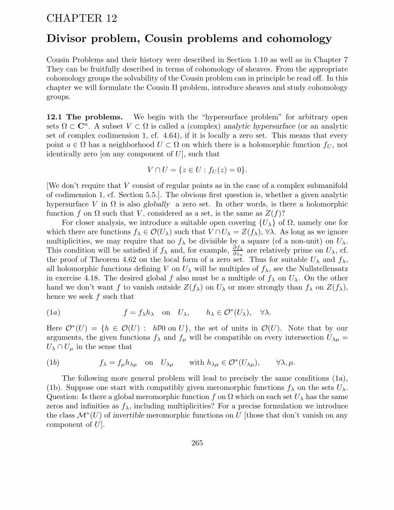
CHAPTER 12

Divisor problem, Cousin problems and cohomology

Cousin Problems and their history were described in Section 1.10 as well as in Chapter 7They can be fruitfully described in terms of cohomology of sheaves. From the appropriatecohomology groups the solvability of the Cousin problem can in principle be read off. In thischapter we will formulate the Cousin II problem, introduce sheaves and study cohomologygroups.

12.1 The problems. We begin with the “hypersurface problem” for arbitrary opensets Ω ⊂ Cn. A subset V ⊂ Ω is called a (complex) analytic hypersurface (or an analyticset of complex codimension 1, cf. 4.64), if it is locally a zero set. This means that everypoint a ∈ Ω has a neighborhood U ⊂ Ω on which there is a holomorphic function fU , notidentically zero [on any component of U ], such that

V ∩ U = z ∈ U : fU (z) = 0.

[We don’t require that V consist of regular points as in the case of a complex submanifoldof codimension 1, cf. Section 5.5.]. The obvious first question is, whether a given analytichypersurface V in Ω is also globally a zero set. In other words, is there a holomorphicfunction f on Ω such that V , considered as a set, is the same as Z(f)?

For closer analysis, we introduce a suitable open covering Uλ of Ω, namely one forwhich there are functions fλ ∈ O(Uλ) such that V ∩Uλ = Z(fλ), ∀λ. As long as we ignoremultiplicities, we may require that no fλ be divisible by a square (of a non-unit) on Uλ.This condition will be satisfied if fλ and, for example, ∂fλ

∂znare relatively prime on Uλ, cf.

the proof of Theorem 4.62 on the local form of a zero set. Thus for suitable Uλ and fλ,all holomorphic functions defining V on Uλ will be multiples of fλ, see the Nullstellensatzin exercise 4.18. The desired global f also must be a multiple of fλ on Uλ. On the otherhand we don’t want f to vanish outside Z(fλ) on Uλ or more strongly than fλ on Z(fλ),hence we seek f such that

(1a) f = fλhλ on Uλ, hλ ∈ O∗(Uλ), ∀λ.

Here O∗(U) = h ∈ O(U) : hν0 on U, the set of units in O(U). Note that by ourarguments, the given functions fλ and fµ will be compatible on every intersection Uλµ =Uλ ∩ Uµ in the sense that

(1b) fλ = fµhλµ on Uλµ with hλµ ∈ O∗(Uλµ), ∀λ, µ.

The following more general problem will lead to precisely the same conditions (1a),(1b). Suppose one start with compatibly given meromorphic functions fλ on the sets Uλ.Question: Is there a global meromorphic function f on Ω which on each set Uλ has the samezeros and infinities as fλ, including multiplicities? For a precise formulation we introducethe classM∗(U) of invertible meromorphic functions on U [those that don’t vanish on anycomponent of U ].

265

DEFINITION 12.11. Let Uλ, λ ∈ Λ be a covering of Ω ⊂ Cn by open subsets. A divisoron Ω associated with Uλ is a system of data

D = Uλ, fλ, λ ∈ Λ,

involving functions fλ ∈ M∗(Uλ) that satisfy the compatibility condition (1b). If inaddition fλ ∈ O(Uλ), ∀λ, one speaks of a holomorphic divisor.

If a holomorphic or meromorphic function f on Ω satisfies the conditions (1a) we say thatit has D as a divisor. A divisor for which there exists an f as in (1a) is called principal.

12.12 MEROMORPHIC SECOND COUSIN PROBLEM or DIVISOR PROBLEM: Let Dbe a divisor on Ω. Is it principal? Or also: Determine a meromorphic function f on Ωwhich has D as a divisor.

Much the same as in the first Cousin problem, one may take the functions hλ of (1a)as unknown. By (1a), (1b) they must satisfy the compatibility conditions hµ = hλhλµwith hλµ ∈ O∗(Uλµ), hence

hλµ = 1/hµλ, hλµ = hλνhνµ

on the relevant intersection of the sets Uα. We thus arrive at the so-called

(HOLOMORPHIC) COUSIN-II PROBLEM or MULTIPLICATIVE COUSIN PROBLEM.Let Uλ, λ ∈ Λ be an open covering of Ω ⊂ Cn and let hλµ, λ, µ ∈ Λ be a family ofzero free holomorphic functions on the (nonempty) intersections Uλ ∩ Uµ that satisfy thecompatibility conditions

(1c)

hλµhµλ = 1 on Uλµ = Uλ ∩ Uµ, ∀λ, µ,

hλµhµνhνλ = 1 on Uλµν = Uλ ∩ Uµ ∩ Uν , ∀λ, µ, ν.

Determine zero free holomorphic functions, hλ ∈ O∗(Uλ), such that

(1d) hµ/hλ = hλµ on Uλµ, ∀λ, µ.

A family of functions hλµ ∈ O∗(Uλµ) satisfying (1c) is called a set of Cousin-II dataon Ω.

Proposition 12.13. A divisor D = Uλ, fλ on Ω belongs to a meromorphic functionF on Ω (in the sense of (1a)) if and only if there is a solution hλ of the holomorphicCousin-II problem on Ω with the data Uλ, hλµ derived from (1b).

The proof is similar to that of Proposition 7.14 for the first Cousin problem.

The Cousin-II problem is the multiplicative analog of Cousin-I. At first glance itmight seem that there is a straightforward reduction of Cousin-II to Cousin-I with the aidof suitable branches of the functions loghλµ. However, the problem is not that easy: evenfor simply connected intersections Uλµ, it is not clear if one can choose branches loghλµ insuch a way that, in conformity with (1c),

(1d) loghλµ + loghµλ = 0, loghλµ + loghµν + loghνλ = 0

266

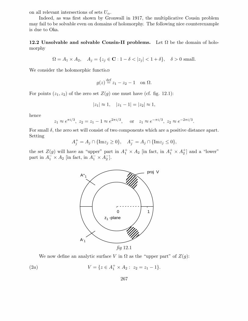
on all relevant intersections of sets Uα.Indeed, as was first shown by Gronwall in 1917, the multiplicative Cousin problem

may fail to be solvable even on domains of holomorphy. The following nice counterexampleis due to Oka.

12.2 Unsolvable and solvable Cousin-II problems. Let Ω be the domain of holo-morphy

Ω = A1 × A2, Aj = zj ∈ C : 1− δ < |zj | < 1 + δ, δ > 0 small.

We consider the holomorphic function

g(z)def= z1 − z2 − 1 on Ω.

For points (z1, z2) of the zero set Z(g) one must have (cf. fig. 12.1):

|z1| ≈ 1, |z1 − 1| = |z2| ≈ 1,

hencez1 ≈ eπi/3, z2 = z1 − 1 ≈ e2πi/3, or z1 ≈ e−πi/3, z2 ≈ e−2πi/3.

For small δ, the zero set will consist of two components which are a positive distance apart.Setting

A+j = Aj ∩ Imzj ≥ 0, A−

j = Aj ∩ Imzj ≤ 0,

the set Z(g) will have an “upper” part in A+1 × A2 [in fact, in A+

1 × A+2 ] and a “lower”

part in A−1 × A2 [in fact, in A−

1 × A−2 ].

0 1

A+1

A-1

proj V

z1 -plane

x x

fig 12.1

We now define an analytic surface V in Ω as the “upper part” of Z(g):

(2a) V = z ∈ A+1 ×A2 : z2 = z1 − 1.

267

12.21 CLAIM. There is no holomorphic function f on Ω which has V as its exact zeroset. In other words, there is no function f ∈ O(Ω) with divisor D = Uj , fj, j = 1, 2 asdefined below:

U1 : a “small” ε-neighborhood of A+1 × A2 in Ω,

f1(z) = z1 − z2 − 1 so that Z(f1) = V ,

U2 : a “small” ε-neighborhood of A−1 × A2 in Ω,

f2(z) = 1 so that Z(f2) = ∅.The corresponding function h12 = f1/f2 on U12 is in O∗. It is claimed that the Cousin-IIproblem for U1, U2 and h12 is unsolvable: h12 can not be written as h2/h1 with hj ∈ O∗(Uj).

PROOF. Suppose on the contrary that there exists f ∈ O(Ω) with divisor D as above, orequivalently, that the corresponding Cousin-II problem has a solution hj, j = 1, 2. Inboth cases we can write

(2b) f = fjhj on Uj , with hj ∈ O∗(Uj), j = 1, 2.

We will obtain a contradiction by comparing the increase of arg f(1, w) along the unitcircle with that of arg f(−1, w). In fact, computation of the difference in the increases byremaining inside U1 will differ from what we get by remaining inside U2. We start withthe latter.

Our f would be in O∗(U2), hence for fixed z1 ∈ A−1 , the function f(z1, w) is holo-

morphic and zero free on A2. There is then a continuous (even holomorphic ) branch oflogf(z1, w) on the open arc C1 = C(0, 1) \ 1. With ∆C1g denoting the increment of galong C1, we have

νf (z1)def=

1

2π∆C1 arg f(z1, w) =

1

2πi∆C1 logf(z1, w) =

1

2πi

∫

C(0,1)

∂f(z1, w)/∂w

f(z1, w)dw.

This integer valued function of z1 is continuous on A−1 , hence constant. In particular

νf (1)− νf (−1) = 0.

We will now compute the same difference via the domain U1. On U1,

f = f1h1 = (z1 − z2 − 1)h1 = gh,

say, where h = h1 ∈ O∗(U1). Thus for h, just as for f before but now remaining inside U1,

νh(1)− νh(−1) = 0.

However, for g(z1, w) = z1 − w − 1 direct calculation gives

νg(z1) =1

2πi

∫

C(0,1)

−1

z1 − w − 1dw =

1 if z1 = 1,

0 if z1 = −1.

Hence, going via U1, we obtain the answer

νf (1)− νf (−1) = νg(1) + νh(1) + νg(−1)− νh(−1) = 1!

This contradiction shows that our divisor problem or Cousin-II problem has no solution:there is no f ∈ O(Ω) with Z(f) = V .

268

REMARK 12.22. The method may be adapted to show that the above Cousin-II problemdoes not even have a continuous solution. That is, there exist no functions gj ∈ C∗(Uj)(zero free continuous functions) such that h12 = g1/g2 on U12. [For merely continuous fone can of course not express νf (z1) by the integral used above.] The non-existence of acontinuous solution suggests a topological obstruction. In fact, Oka proved a result on theholomorphic divisor problem akin to the following

Theorem 12.23. Let Ω ⊂ Cn be a Cousin-I domain. The Cousin-II problem on Ω withcompatible data Uλ, hλµ has a holomorphic solution if and only if it has a continuoussolution.

PROOF. We only give an outline since we will prove a more refined result later on.(i) Just as in the case of Cousin-I the given Cousin-II problem will be solvable if and only

if its refinements are solvable (cf. Proposition 7.32).(ii) Refining our problem, if necessary, we assume that the sets Uλ, and hence the inter-

sections Uλµ, are convex. On a convex set a zero free holomorphic (or continuous)function has a holomorphic (or continuous) logarithm, cf. Proposition 12.72 below.

(iii) Supposing now that our original Cousin-II problem has a solution, the same is truefor the refined problem. That is, if we denote the (possibly) refined data also byUλ, hλµ, there exist functions gλ ∈ C∗(Uλ) such that hλµ = gµ/gλ on Uλµ, for allλ, µ. Choosing continuous logarithms loggλ on the sets Uλ, we then define

loghλµ = loggµ − loggλ on Uλµ, ∀λ, µ.

Since hλµ is holomorphic and loghλµ continuous, loghλµ will be holomorphic on Uλµ.Indeed, loghλµ will have local representations similar to (7a) below.The present functions loghλµ will automatically satisfy the compatibility conditions

(1d) for the additive Cousin problem. Thus since Ω is a Cousin-I domain, there existfunctions ϕλ ∈ O(Uλ) such that

loghλµ = ϕµ − ϕλ on Uλµ, ∀λ, µ.

It follows thathλµ = eϕµ/eϕλ on Uλµ,

that is, the Cousin-II problem is solved by the functions hλ = eϕλ ∈ O∗(Uλ).

Theorem 12.23 is an example of the heuristic “Oka principle”: If a problem on adomain of holomorphy is locally holomorphically solvable and if it has a global continuoussolution, then it has a global holomorphic solution.

12.3 Sheaves. Sheaves were introduced and studied by Cartan, Leray and Serre. Theywere used by Cartan and Grauert in connection with the solution of the Levi-problem.Sheaves have been a highly successful tool in several parts of mathematics, particularly inalgebraic geometry. Examples of sheaves are scattered all over this book. It is high timewe formally define them.

269

DEFINITION 12.31. A sheaf F over a space X with projection π is a triple (F , π,X)where F and X are topological spaces and π is a surjective local homeomorphism.

A section of (F , π,X) over an open U ⊂ X is a continuous map σ : U → F such that σ πis the identity mapping on U . The sections over U are denoted by F(U) or Γ(U) = Γ(U,F).A stalk of (F , π,X) is a subset of F of the form π−1(x) where x ∈ X.

A sheaf of rings, (abelian) groups, etc. is a sheaf F with the property that thestalks F(x) have the structure of a ring, respectively, an (abelian) group, etc. of which thealgebraic operations like addition or multiplication are continuous. The latter means thefollowing: form the product space F × F with product topology and consider the subset

F · F = (f1, f2) ∈ F × F : π(f1) = π(f2).Now addition (for example) in the stalks of F gives rise to a map

+ : F · F → F , (f1, f2) 7→ f1 + f2,

which has to be continuous.

EXAMPLES 12.32. Let D be a domain in Cn.(i) The constant sheaves C × D, Z × D, etc. over D. Projection is ordinary projection

on D. Observe that C (and Z etc.) need be equipped with the discrete topology.(ii) The Riemann domains (R, π,D) of Definition 2.12 equipped with the usual topology,

that is, defined by the basic neighborhoods N (p, V, g).(iii) The sheaf of germs of holomorphic functions on U , denoted by OU , with projection

π : [f ]a 7→ a. Here [f ]a denotes the germ of an analytic function f at a pointa ∈ U . For OU to become a sheaf we have to give it a topology that makes π a localhomeomorphism. This can be done in a way similar to example (ii): A base for thetopology is given by the sets

(3a) N (V, f) = [f ]a : a ∈ V where f ∈ O(V ).

Sections over V can be identified with holomorphic functions on V : To a holomorphicfunction f on V we associate the section

σf : a 7→ [f ]a.

It is an easy exercise to check that σ is continuous. The fact that O(V ) indicates bothsections over V and holomorphic functions on V reflects this association.

(iv) Let K denote an algebra of functions on U . Thus K could be C∞(U) or ∧p,q(U) the(p, q)-forms on U (our functions may well be vector valued!) A germ of a function inK was defined in Section 2.1. As in the previous example these germs together forma sheaf a base for the topology of which is given similar to (3a). We thus obtain thesheaf C∞

U of germs of smooth functions on U , the sheaf ∧p,qU of germs of smooth p, qforms on U , the sheaf O∗

U of holomorphic zero free functions on U , the sheaf MU ofgerms of meromorphic functions on U (strictly speaking this one does not consists ofgerms of functions), etc. Again sections and functions can be identified.

It is easily seen that the examples (i, iii, iv) have the property that the stalks areabelian groups or have even more algebraic structure. We leave it to the reader to checkthat the algebraic operations are continuous.

We need some more definitions.

270

DEFINITION 12.33. Let F and G be sheaves over X with projections πF , respectivelyπG . A continuous map ϕ : F → G is called a sheaf map if

πF = πG ϕ.

G is called a subsheaf of F if for all x ∈ X we have Gx ⊂ Fx. If F and G are sheaves ofabelian groups then a map of sheaves ϕ : F → G is called a sheaf homomorphism if itsrestriction to each stalk is a group homomorphism. Similarly one defines homomorphismsof sheaves of rings, etc.

Observe that a sheaf homomorphism ϕ : F → G induces homomorphisms ϕ∗ : F(U) →G(U), ϕ∗(σ) = ϕ σ for σ ∈ F(U).

12.4 Cohomological formulation of the Cousin-problems. Cousin-I and Cousin-IIdata hλµ associated with an open covering Uλ of Ω ⊂ Cn are examples of so-calledcocycles consisting of sections in the sheaves O and O∗ over Ω. These are sheaves of abeliangroups. The group operation will always be denoted by + (it is multiplication of germsin case of O∗!). In this section we will deal with Cousin problems associated to arbitrarysheaves of abelian groups over domains in Cn

12.41. GENERAL COUSIN PROBLEM. Suppose we have a open covering U = Uλ,λ ∈ Λ of Ω ⊂ Cn. For a sheaf of abelian groups F over Ω, Cousin data associated with Uconsist of sections fλµ of F , one over each intersection Uλµ, λ, µ ∈ Λ, such that

(4a) fλµ + fµλ = 0,

(4b) fλµ + fµν + fνλ = 0

on the relevant intersections of sets Uα. One tries to determine a family of sections fλ ∈Γ(Uλ,F), (λ ∈ λ), such that

(4c) fλµ = fµ − fλ on Uλµ, ∀λ, µ.

We introduce some further terminology. With a covering U = Uλ of Ω there are associ-ated various cochains “with values in” F .

DEFINITION 12.42. (Cochains for U with values in F). A zero-cochain f 0− is a family

of sections fλ, fλ ∈ Γ(Uλ). It is simply a function on Λ assuming specific sections of Fas values:

f0− : λ 7→ f0

λ ∈ Γ(Uλ), λ ∈ Λ.

A 1-cochain f1− is a family of sections fλµ, fλµ ∈ Γ(Uλµ) with the alternating property

(4a). It is an alternating function on Λ2:

f1− : (λ, µ) 7→ f1

λ,µ ∈ Γ(Uλµ), λ, µ ∈ Λ.

271

An s-cochain f s− is an alternating function on Λs+1:

fs− : (λ0, λ1, . . . , λs) 7→ fsλ0λ1...λs∈ Γ(Uλ0λ1...λs

), λj ∈ Λ.

Here Uλ0λ1...λs= Uλ0

∩ . . . ∩ Uλs, while alternating means that for a permutation σ with

sign ε(σ) we have f sσ(λ0λ1...λs) = ε(σ)fsλ0λ1...λs.

For s-cochains associated to U one defines addition as addition of the values of the cochain.Thus one obtains the abelian group of s-cochains:

Cs(U) = Cs(U ,F).

Starting with a 0-cochain f 0− for U , formula (4c) defines a 1-cochain f 1

− which isdenoted by δf0

−. We need a corresponding operator on s-cochains:

δ = δs : Cs(U)→ Cs+1(U).

DEFINITION 12.43 (Coboundary operator). For an s-cochain f s− = fλ0λ1...λs one de-

fines δfs− ∈ Cs+1(U) by

(δfs−)λ0λ1...λs+1=

s+1∑

r=0

(−1)rfλ0...λr ...λson Uλ0λ1...λs+1

, ∀(λ0, λ1, . . . λs+1),

where λr means that the index λr is omitted.

Observe that δ is a homeomorphism.

Illustration. The Cousin data in (12.41) consist of a 1-cochain f 1− = fλµ for U with

values in F ((4a)), such that δf 1− = 0 ((4b)). The Cousin problem is whether there exists

a 0-cochain f0− for U with values in F such that f 1

− = δf0− ((4c)).

DEFINITION 12.44 (Cocycles and coboundaries for U and F). An s-cochain f s− is calledan s-cocycle if

δfs− = 0.

An s-cochain f s− is called a s-coboundary if (s ≥ 1 and)

fs− = δfs−1− ,

for some (s− 1)-cochain f s−1− .

Because δ is a homomorphism, the s-cocycles form a subgroup

Zs(U) = Zs(U ,F) ⊂ Cs(U ,F);

Similarly the s-coboundaries form a subgroup

Bs(U) = Bs(U ,F) ⊂ Cs(U ,F).

272

Lemma 12.45. Every s-boundary is an s-cocycle:

δ2 = δsδs−1 = 0, s ≥ 1,

hence Bs(U) is a subgroup of Zs(U).

PROOF. This is a verification similar to the one for the ∂ operator.

(δsδs−1fs−1− )λ0λ1...λs+1

=

s+1∑

r=0

(−1)r(δs−1fs−1− )λ0...λr...λs+1

=s+1∑

r=0

(−1)rr−1∑

k=0

(−1)kfs−1

λ0...λk...λr...λs+1

+s+1∑

r=0

(−1)rs+1∑

k=r+1

(−1)k−1fs−1

λ0...λr ...λk...λs+1

= 0,

because of cancelation.The case s = 0 is somewhat special: there are no real coboundaries and one defines

B0 = 0. For a 0-cocycle f 0− = fλ one has

fµ − fλ = 0 on Uλµ, ∀λ, µ.

Apparently a 0-cocycle determines a global section of F : one may define f ∈ Γ(Ω,F) in aconsistent manner by setting

f = fλ on Uλ, ∀λ.

In this setup the groups Cs(U ,F) form what is called a semi-exact sequence or com-plex:

(4d) · · · δ−→Cs−1(U ,F)δ−→Cs(U ,F)

δ−→Cs+1(U ,F)δ−→· · · . (δ δ = 0)

This notion makes sense for sequences of abelian groups connected through homo-morphisms with the property that the composition of two consecutive ones is 0. Thus asemi-exact sequence of abelian groups is a sequence

· · ·−→Ajfj−→Aj+1

fj+1−→Aj+2−→· · ·

with fj+1 fj = 0. If, moreover, the kernel of fj+1 equals the image of fj , the sequenceis called exact. The same terminology applies to sequence of sheaves of abelian groupsconnected through sheaf homomorphisms. Finally, a short exact sequence is an exactsequence of the form

0→ Af−→B

g−→C → 0.

It follows that here f is injective, while g is surjective.The important objects are the quotient groups of (4d):

273

DEFINITION 12.46 ((v)Cech Cohomology groups for U and F). The quotient group

Hs(U ,F)def=Zs(U ,F)

Bs(U ,F)=

s-cocycles

s-coboundaries

is called the s-th cohomology group for the covering U of Ω with values in F . The elementsare equivalence classes of s-cocycles, the cosets of the subgroup of s-coboundaries.

For s = 0 one has

(4e) H0(U ,F) = Z0(U ,F) = Γ(Ω,F).

The cohomology groups are zero if and only if (4d) is exact. They measure the “amountof inexactness” of the complex.

ILLUSTRATION The Cousin problem asks if a given 1-cocycle f 1− for U and F is a

1-coboundary. Thus this Cousin problem is always solvable when every 1-cocycle is a1-coboundary, in other words when

H1(U ,F) = 0.

EXAMPLE 12.47. [cf. Example (7.17)]. Take F = O, Ω = C2 − 0, Uj = zjν0, j =1, 2. The associated 0-cochains h0

− = h1, h2 are given by the holomorphic functions

hi(z) =∑

α∈Z2

aiαzα on Ui (i = 1, 2),

with aiα = 0 if α1−i < 0. The 1-cochains h1− = h11, h12, h21, h22 are given by holomorphic

functions

(4f) h11 = h22 = 0, h12(z) = −h21(z) =∑

α∈Z2

cαzα on U12.

The relations in (4f) follow from the alternating property of cocycles. The 1-cochains areat the same time 1-cocycles since there are only two different indices:

(δh1−)jkl = hkl − hjl + hjk = 0

whenever two indices such as k and l are the same.

The 1-coboundaries are those 1-cocycles, for which h12 on U12 equals a difference h2 − h1

of functions hj ∈ O(Uj). That is, (4f) represents a coboundary if and only if

cα = a1α − a2

α, ∀α ∈ Z2.

This requirement presents no problem if α1 ≥ 0 or α2 ≥ 0 (or both). However if α1, α2 < 0there is no solution unless cα = 0 Thus the coboundaries are those cocycles with cα = 0,

274

(αi < 0). The cohomology group H1(U ,O) is isomorphic to the group of holomorphicfunctions

h12(z) =∑

αi<0

cαzα on U12.

EXAMPLE 12.48. Taking F and Ω as above, we consider the covering V1 = 0 < |z| < 2,V2 = 1 < |z| < ∞. The associated Cousin problem will be generally solvable. Indeedevery holomorphic function h12 on V12 = 1 < |z| < 2 has an analytic continuationto B(0, 2) [by Hartogs’ spherical shell theorem, Sections 2.8, 3.4]. Thus such a functionis written as h12 = 0 − h1 with h1 the analytic continuation to V1 of h12. Conclusion:H1(V1, V2,O) = 0.

12.5 Definition of the domain cohomology groups Hs(Ω,F). The illustration to(12.46) gives the precise condition H1(U ,F) = 0 for the general solvability of the Cousinproblem for F and a fixed covering U of Ω. We would also like to have a condition on Ωwhich assures the general solvability of the Cousin problem for every covering of Ω. [Forthe sheaf O such a condition was that Ω be a ∂ domain, cf. Chapter 7.] Keeping F fixedwe write

Hs(U ,F) = Hs(U).

By Proposition 7.32 whose proof is valid for general sheaves F , refinement of Cousin datadoes not affect the solvability of the Cousin problem, Thus if V is a refinement of U andH1(V) = 0, so that all Cousin problems for V are solvable, then in particular all refinementsto V of Cousin problems for U are solvable, hence all Cousin problems for U are solvableso that H1(U) = 0.

What will happen in general to the cohomology groups if we refine the covering U of Ωto V? We will see that H1(U) is always (isomorphic to a subgroup of H1(V). Refinementmay lead to large and larger groups H1(W) which ultimately become constant. The limitgroup is called H1(Ω,F). For s ≥ 2 the situation is more complicated; in the generalcase one needs the notion of a direct limit to define Hs(Ω,F), see below. We need twopropositions

Proposition 12.51. A refinement of the covering U of Ω to V via a refinement map σinduces a unique homomorphism σ∗ = σ(U ,V) of H(U) to H(V), that is a sequence ofhomomorphisms σ∗

s(U ,V) : Hs(U)→ Hs(V). Uniqueness means here that the homomor-phism is independent of the choice of the refinement map.

PROOF. Let the covering V = Vj, j ∈ J , of Ω be a refinement of the covering U = Uλ,λ ∈ Λ and let σ : J → Λ be a refinement map, that is, every set Vj is contained in Uσ(j).To every cochain f s− ∈ Cs(U) the map assigns a cochain in Cs(V) — denoted by σ(f s−) —by restriction. Specifically, for s = 0, 1, . . ., we have, with σ = σs,

σ(fs−)j0j1...js = fsσ(j0)σ(j1)...σ(js) | Vj0j1...js .The maps σ on cochain groups are clearly homomorphisms. Moreover they commute

with the coboundary operator δ:

δs σs = σs+1 δs, (Cs(U)→ Cs+1(V)).

275

Thus, the image of a cocycle is again a cocycle and the image of a coboundary is acoboundary, that is, σs maps Zs(U) into Zs(V) and the subgroups Bs(U) into Bs(V). Itfollows that σ induces a homomorphisms σ∗

s of the quotient groups by σ∗s : [fs−] 7→ [σfs−],

in other words, we found a homomorphism

σ∗ : Hs(U)→ Hs(V).

We will now indicate how to show that σ∗ depends only on the refinement and noton the refinement map. Here the notion of a chain homotopy is useful. Suppose that σand τ are two (chain) homomorphism from the complexes C(U) to C(V) associated tothe refinement mappings σ and τ . A chain homotopy between σ and τ is a (sequence of)map(s)

Θ = Θs, Θs : Cs(U)→ Cs−1(V), (s = 1, 2, . . .).

with the property that

(5a) Θs+1δs + δs−1Θs = (σs − τs).

Assuming that Θ has been constructed, suppose that fs is an s-cocycle. Then δfs = 0 and(5a) gives (σs − τs)fs = δs−1Θsfs, which is a coboundary. Thus σ∗ = τ∗.

Now we have to define Θ:

(5b) [Θsfs−]j0j1...js−1

=s−1∑

r=0

(−1)rfτ(j0)τ(j1)...τ(jr)σ(jr)...σ(s−1).

Verification of (5b) is a tedious calculation. However, if we can prove that (5b) defines achain homotopy for those τ and σ which are equal on J − k for one k ∈ J , then we aredone, because we can deform two arbitrary refinement maps to each other by a chain ofdeformations, changing one j ∈ J at a time. Now if τ(j) = σ(j) on J − k, then there aretwo possibilities

i. k is not in j0, . . . js. Then (σs − τs)(fj0...js) = 0 and (5b) equals 0 so we are done.ii. k is in j0, . . . js. We may assume k = j0. We find

(σs − τs)(fj0...js) = fσ(j0)...σ(js) − fτ(j0)...τ(js).

To verify (5b) we compute, keeping in mind that fλ0...λs= 0 if two indices are equal,

[δΘsfs−]j0j1...js =

s∑

l=0

(−1)l[Θsfs−]j0j1...jl...js = +

s∑

l=1

(−1)lfsτ(j0)σ(j0)σ(j1)...jl...σ(js−1)

and

[Θs+1δfs−]j0j1...js = [δf ]τ(j0)σ(j0)...js

= (σs − τs)(fj0...js) +

s∑

l=1

(−1)l+1fsτ(j0)σ(j0)σ(j1)...jl...σ(js−1).

Adding yields (5b).

276

Proposition 12.52. For s = 1 the homomorphism σ∗ = σ(U ,V) in Proposition 12.51 isinjective, hence if V is a refinement of U then H1(U) is isomorphic to a subgroup of H1(V).

PROOF. Let f1− be an arbitrary cocycle in Z1(U), with cohomology class [f 1

−] ∈ H1(U).Supposing that σ∗[f1

−] = [σf1−] = 0 in H1(V), we have to show that [f 1

−] = 0. But thisfollows from (the proof of) Proposition 7.32 on refinements of Cousin problems. Indeed ifσf1

− is a coboundary for V, the refined Cousin problem for V and σf 1− is solvable, but then

the original Cousin problem for U and f 1− is also solvable, so that f 1

− is a coboundary forU .

DEFINITION 12.53. The (domain) cohomology group Hs(Ω) = Hs(Ω,F) is the “directlimit” of the (coverings) groups Hs(U) = Hs(U ,F) under the mappings σ(U ,V), associatedwith all possible refinements of coverings U of Ω to coverings V. The direct limit may bedefined as the set of equivalence classes of elements in the disjoint union ∪UHs(U) over allcoverings U of Ω. Elements u ∈ Hs(U) and v ∈ Hs(V) are equivalent if there is a commonrefinement W of U and V such that u and v have the same image in Hs(W), that is,

σ∗(U ,W)u = σ∗(V,W)v.

Every element of [u] of Hs(Ω) has a representative u in some group Hs(U). For anyrefinement W of this U the class [u] will contain the element σ(U ,W)u of Hs(W). Thesum of two elements [u] and [v] in Hs(Ω), where u ∈ Hs(U) and v ∈ Hs(V) is formedby adding the representatives σ(U ,W)u and σ(V,W)v in Hs(W), where W is a commonrefinement of U and V.

By Propositions 12.51 and 12.52 we have the following important

COROLLARY 12.54. The map u ∈ Hs(U) 7→ [u] ∈ Hs(Ω) defines a homomorphism ofHs(U) into Hs(Ω) and for s = 1 this homomorphism is injective. In particular H1(U) isisomorphic to a subgroup of H1(Ω) and H1(Ω,F) = 0 (The Cousin problem for Ω withvalues in F is solvable) if and only if H1(U ,F) = 0 for every covering U of Ω.

REMARK. One may also think of the elements of Hs(Ω) as equivalence classes of cocyclesin the disjoint union ∪UZs(U) over all coverings U of Ω. To this end one extends the notionof cohomologous cocycles to cocycles belonging to different coverings: f s− ∈ Zs(U) andϕs− ∈ Zs(V) are called equivalent or cohomologous in ∪UZs(U) if they have cohomologousimages in Zs(W) for some common refinement W of U and V. Observe that a commonrefinement of U and W always exists: Take

W = W = U ∩ V : U ∈ U , V ∈ V.

12.6 Computation of H(Ω,F) and in particular H1(Ω,O). We first prove a generalresult on the computation of H1(Ω) = H1(Ω,F).

277

Theorem 12.61. Let U = Uλ, λ ∈ Λ be any covering of Ω ⊂ Cn by Cousin domainsfor F : H1(Uλ,F) = 0 for all λ. Then

H1(Ω,F) ∼= H1(U ,F).

PROOF. We have to show that H1(W) is (isomorphic to) a subgroup of H1(U) for everycovering W of Ω, so that H1(U) is maximal and thus equal to H1(Ω). Now H1(W) is asubgroup of H1(V) for any common refinement V of U and W [Proposition 12.52], henceit is sufficient to show that

(6a) H1(V) ∼= H1(U) for all refinements V of U .

Choose a refinement V = Vj, j ∈ J of U and an associated 1-cocycle ϕ1− = ϕjk.

Restriction of ϕ1− to Uλ gives a 1-cocycle (also denoted by ϕ1

−) on Uλ for the coveringVj ∩ Uλ, j ∈ J . By the hypotheses this cocycle is a coboundary: we can choose a0-cochain ϕ0

−λ or ϕλ− on Uλ such that

ϕjk = ϕλk − ϕλj on Vjk ∩ Uλ, ∀j, k.

We do this for all λ; on Uµ we find

ϕjk = ϕµk − ϕµj on Vjk ∩ Uµ, ∀j, k.

Thus on Uλµ ∩ Vjk, ϕµk − ϕλk = ϕµj − ϕλj , so that we may define fλµ in a consisted manneron Uλµ by setting

(6b) fλµ = ϕµj − ϕλj on Uλµ ∩ Vj , ∀j ∈ J.

One readily verifies that (6b), ∀λ, µ ∈ Λ defines a 1-cocycle f 1− for the covering U .

For given ϕ1−, this cocycle may depend on the choices of the 0-cocycle ϕλ−. However, if we

make different choices ψλ− then ψλk − ψλj = ϕλk − ϕλj , hence the differences ψλj − ϕλj define

a 0-cochain g− for U via gλ = ψλj − ϕλj on Uλ ∩ Vj , ∀j. The result is that f1− is replaced

by the cohomologous cochain f1− = f1

− + δg−:

fλµ − fλµ = ψµj − ψλj − (ϕµj − ϕλj ) = gµ − gλ on Uλµ ∩ Vj , ∀j.

Thus by our process, the cohomology class of f 1− in Z1(U) is uniquely determined by ϕ1

−.Note also that coboundaries go into coboundaries: for a coboundary ϕ1

− we may take the0-cochains ϕ0

−λ equal to ϕ0− independent of λ and we then obtain f 1

− = 0! Thus we havea map of cohomology classes belonging to Z1(V) into cohomology classes belonging toZ1(U) and this map is a homomorphism. The map is injective too: if f 1

− is a coboundary,fλµ = fµ − fλ, (6b) shows that the definition χj = ϕλj − fλ, ∀λ gives a 0-cochain χ− for Vand ϕ1

− = δχ−.The conclusion is that our process defines an injective homomorphism of H1(V) into

H1(U), hence H1(V) is a subgroup of H1(U). Since conversely H1(U) is a subgroup ofH1(V) [Proposition 12.52], the proof of (6a) is complete.

278

EXAMPLE 12.62. For Ω = C2−0 one may compute H1(Ω,O) with the aid of example(12.47).

Theorem 12.61 is a special case of the following theorem of J. Leray, a proof of which can befound in [GuRo], or [GrRe]. Call a covering Uλ of Ω ⊂ Cn acyclic if Hs(Uλ1...λj

,F) = 0for all s ≥ 1 and for all intersections Uλ1...λj

.

Theorem 12.63 (Leray). For every acyclic covering U of Ω:

Hs(Ω,F) ∼= Hs(U ,F), s = 0, 1, 2, . . . .

In the case of the first Cousin problem, (F = O), we have general solvability for allcoverings U of Ω ⊂ Cn if and only if H1(Ω,O) = 0. By Chapter 7 we also have generalsolvability if and only if the equation ∂u = v on Ω is generally C∞ solvable for all (0,1)-forms v (of class C∞) for which ∂v = 0. Recall that (the sheaf of sections of) (p, q) formson Ω is denoted by ∧p,q = ∧p,q(Ω).

For p = 0, 1, . . . we have an exact sequence of sheaves

(6c) 0→ Op,0 i−→∧p,1 ∂−→∧p,2 ∂−→· · · ∂−→∧p,n → 0.

Here Op,0 is the subsheaf of ∧p,0 consisting of germs (p, 0) forms with holomorphic co-effients; O0,0 = O. Exactness follows from the fact that ∂∂ = 0 and that locally, forexample on polydiscs (Section 7.6, Chapter 11), the equation ∂u = v, has a solution if∂v = 0. To (6c) is associated a semi-exact sequence of the groups of sections, that is, thegroups of smooth differential forms on Ω:

(6d) 0→ Op,0(Ω)i−→∧p,1(Ω)

∂−→∧p,2 (Ω)∂−→· · · ∂−→∧p,n (Ω)→ 0.

In general (6d) is not exact, globally the equations ∂u = v, may not have a solution even if∂v = 0. Again cohomology groups will measure the amount of inexactness. See Definition12.68 below.

Before pursuing this any further we will compute some trivial cohomology groups.We have seen in Chapter 7 that it is useful to be able to solve smooth Cousin-I problems,in order to connect them to the Cauchy-Riemann equations. Now we will do somethingsimilar in terms of cohomology. First we introduce some terminology.

DEFINITION 12.64. Let Ω ⊂ Cn and let U be an open covering of Ω and F a sheafof abelian groups over Ω. A partition of unity of F subordinate to U is a set of sheafhomomorphisms βλ : F → F such that

i.∑

λ βλ = id on F ;ii. βλ([f ]x) = [0]x for all x in some open neighborhood of the complement of Uλ.

EXAMPLES 12.65. Let U be a covering of Ω ⊂ Cn and let βλ be a (usual) partitionof unity subordinate to U . Then the βλ give rise to a partition of unity βλ of the sheafC∞ on Ω by

βλ([u]z) = [βλu]z.

Similarly ∧p,q(Ω) admits a partition of unity subordinate to U .

279

DEFINITION 12.66. A sheaf of abelian groups F over Ω is called fine if for every (locallyfinite) covering U of Ω it admits a partition of unity subordinate to U .

The sheaves in 12.65 are fine sheaves.

Theorem 12.67. Suppose that F is a fine sheaf over Ω and that U is any locally finitecovering of Ω. Then Hp(Ω,U) = 0, (p ≥ 1), for every U and therefore Hp(Ω,F) = 0 forp ≥ 1.

PROOF. Let U = Uλ be a locally finite covering of Ω and let βλ be the associatedpartition of unity of F . It suffices to show that for p > 0 every p-cocycle (for U and F) isa p-coboundary. This is done similarly to the proof of Theorem 7.41. Let σ− ∈ Zp(U ,F).Put

τλ0···λp−1=∑

µ

βµ(σµλ0···λp−1).

Notice that βµ(σµλ0···λp−1) is at first only defined on Uµ ∩ Uλ0···λp−1

, but extends toUλ0···λp−1

because it vanishes in a neighborhood of the boundary of Uµ. Thus τ is awell defined (p− 1) cocycle. We compute

(δτ)λ0···λp=

p∑

i=0

(−1)iτλ0···λi···λp=

p∑

i=0

(−1)i∑

µ

βµ(σµλ0···λi···λp)

=∑

µ

βµ

(

p∑

i=0

(−1)iσµλ0···λi···λp

)

=∑

µ

βµ(σλ0···λp) = σλ0···λp

,

where we have used that σ is a cocycle, i.e.∑p+1

i=0 (−1)iσλ0···λi···λp+1= 0, for all indices λi,

in particular with λ0 = µ, and that∑

µ βµ = id.

DEFINITION 12.68. Forms v with ∂v = 0 are called ∂ closed, forms v = ∂u are called ∂exact. Let Zp,q

∂(Ω) denote the group of ∂ closed forms in ∧p,q(Ω) and let Bp,q

∂(Ω) denote

the group of ∂ exact forms in ∧p,q(Ω). The quotient groups are the Dolbeault cohomologygroups:

Hp,q

∂(Ω)

def=Zp,q∂

(Ω)

Bp,q∂

(Ω).

Thus general solvability of the first Cousin problem may also be expressed by the conditionH0,1(Ω) = 0. As a consequence H1(Ω,O) = 0 if and only if H0,1

∂(Ω) = 0. Much more is

true:

Theorem 12.69 (Dolbeault). Let Ω ⊂ Cn be open and let U be a locally finite coveringof Ω that consists of domains of holomorphy. Then for p = 0, 1, . . . , n

Hq(Ω,O) = H0,q

∂(Ω) = Hq(U ,O).

For the proof we need some results from homological algebra. Let

0→ E i−→F s−→G → 0

280

be an exact sequence of sheaves over Ω. For U open in Ω there is an associated exactsequence of groups of sections

(6e) 0→ E(U)i∗−→F(U)

s∗−→G0(U)→ 0.

Here G0(U) denotes the image of F(U) under s∗ in G(U), which need not be all of G(U).Similarly, if U is an open covering of Ω, then there is an induced exact sequence of chaingroups with Cs0(U ,G) the image of s∗ in Cs(U ,G):

(6e′) 0→ Cs(U , E)i∗−→Cs(U ,F)

s∗−→Cs0(U ,G)→ 0.

See exercise 12.11.The coboundary operator δ commutes with the maps i∗ and s∗. One thus obtains the

following commutative diagram with exact columns.

(6f)

0 0 0

y

y

y

· · · δ−→ Cs−1(U , E)δ−→ Cs(U , E)

δ−→ Cs+1(U , E)δ−→· · ·

y

ϕ

y

ϕ

y

ϕ

· · · δ−→ Cs−1(U ,F)δ−→ Cs(U ,F)

δ−→ Cs+1(U ,F)δ−→· · ·

yψ

yψ

yψ

· · · δ−→ Cs−10 (U ,G)

δ−→ Cs0(U ,G)δ−→ Cs+1

0 (U ,G)δ−→· · ·

y

y

y

0 0 0

.

Commutative means, of course, that every two possible compositions of maps originatingat the same group and ending in the same group yield the same map. The maps ϕ and ψcommute with δ and therefore (compare the proof of Proposition 12.51) take cocycles tococycles, coboundaries to coboundaries. Thus ϕ and ψ induce homomorphisms ϕ∗, ψ∗:

(6g) Hs(U , E)ϕ∗

−→Hs(U ,F)ψ∗

−→Hs0(U ,G), s = 0, 1, 2 . . .

The various sequences (6g) are connected through a homomorphism induced by δ:

Proposition 12.610 (Snake Lemma). Associated to the commutative diagram (6f)there exist connecting homomorphisms δ∗ : Hs

0(U ,G)→ Hs+10 (U , E) for the sequences (6g)

such that the following sequence is exact:

0−→H0(U , E)ϕ∗

−→H0(U ,F)ψ∗

−→H00 (U ,G)

δ∗−→H1(U , E)ϕ∗

−→H1(U ,F)ψ∗

−→H10 (U ,G)

δ∗−→H2(U , E)ϕ∗

−→H2(U ,F)ψ∗

−→H20 (U ,G)

δ∗−→· · · .

281

PROOF. We define δ∗ by chasing through the diagram. Take a cocycle g ∈ Zs(U ,G).The map ψ is surjective, hence there exists f ∈ Cs(U ,F) with ψf = g. Observe thatψδf = δψf = δg = 0, thus δf ∈ Cs+1(U ,F) belongs to the kernel of ψ and as ϕ isinjective, ∃! e = e(f) ∈ Cs+1(U , E) such that δf = ϕe. We compute ϕδe(f) = δδf = 0,hence, because ϕ is injective, e(f) ∈ Zs+1(U , E). Now we wish to define δ∗[g] = [e(f)].

We have to check that this is well defined, that is, independent of the choice of f inthe class [f ] and, moreover, that if g is a coboundary, e is a coboundary too.

Suppose ψ(f − f) = 0. Then f − f = ϕes so that δ(f − f) = ϕδes. In other wordse(f)− e(f) = δes, that is [e(f)] = [e(f)].

Next suppose that g = δgs−1 is a coboundary. Then gs−1 = ψfs−1 for some fs−1 ∈Cs−1(U ,F). Also gs = ψfs. Now observe that ψ(fs−δfs−1) = 0, so that fs−δfs−1 = ϕes.We obtain that δfs = δ(fs − δfs−1) = δϕes = ϕδes. We conclude that e(f) = δes acoboundary.

Finally we show exactness of the sequence. This is again done by chasing the diagram(6f).

At Hp(U, E). [ep] ∈ im δ∗ ⇔ ∃fp−1 : δψfp−1 = 0 and ϕep = δfp−1 ⇔ [ϕep] = 0.At Hp(U,F). [fp] ∈ kerψ∗ ⇔ ∃gp−1 : ψfp = δgp−1 ⇔ ∃fp−1 : δψfp−1 = ψδfp−1 =

ψfp ⇔ ∃fp−1 : ψ(fp − δfp−1) = 0⇔ ∃fp−1 : fp + δfp−1 ∈ imϕ⇔ [fp] ∈ imϕ∗

At Hp0 (U,G). δ∗[gp] = 0⇔ ∃fp : ψfp = gp and [ϕ−1δfp] = 0⇔ ∃epϕ−1δfp = δep ⇔

δ(fp − ϕe) = 0⇔ f − ϕe ∈ Zp(U ,F) and ψ∗[f − ϕe] = [ψf ] = [g].

Now we wish to pass to the direct limit and also replace C0 by C in the exact sequence.We need

Lemma 12.611. Keeping the notation as before, suppose that g− ∈ Cp(U ,G). Thenthere exists a refinement V of U with refinement map σ such that the refined cochain gσis in Cp0 (V,G).

PROOF. After refinement if necessary, we may assume that U is a special open coveringin the sense of 7.33 and that there is an open covering W = Wλ with the property thatWλ ⊂ Uλ. Let gλ0···λp

be a p cochain in Cp(U ,G). Because the sequence (6e) is exact, thereexists for every z ∈ Ω and every λ0 · · ·λp with z ∈ Uλ0···λp

a neighborhood Vz ⊂ Uλ0···λp

such that gλ0···λp| Vz = s fλ0···λp

| Vz for some fλ0···λpdefined on Vz. For a fixed z there

are only finitely many intersections Uλ0···λpthat contain z, because the covering is locally

finite. Thus we may choose Vz independent of λ0 · · ·λp. Shrinking Vz if necessary, we mayalso assume that Vz ∩Wλ 6= ∅ implies that Vz ∈ Uλ and z ∈ Wλ implies that Vz ∈ Wλ.From Vzz∈Ω we select a countable, locally finite subcovering Vi = Vzi

and we define therefinement function σ by choosing σ(i) ∈ λ : z ∈Wλ. Suppose that Vi0···ip is nonempty.Then for 0 ≤ j ≤ p Vi0∩Wσ(ij) 6= ∅, hence Vi0 ⊂ Uσ(ij). Now the refined cochain σ(g)i0··· ipis the restriction of the function gσ(i0)···σ(ip) defined on Uσ(i0)···σ(ip) ⊃ Vi0 , and thereforethere exists f = fσ(i0)···σ(ip) on Vi0 with s f = g on Vi0···ip .

COROLLARY 12.612 (Snake Lemma). The following sequence is exact

0−→H0(Ω, E)ϕ∗

−→H0(Ω,F)ψ∗

−→H0(Ω,G)δ∗−→H1(Ω, E)

ϕ∗

−→H1(Ω,F)ψ∗

−→H1(Ω,G)δ∗−→H2(Ω, E)

ϕ∗

−→H2(Ω,F)ψ∗

−→H2(Ω,G)δ∗−→· · · .

282

PROOF. Lemma 12.611 and the fact that δ commutes with refinement maps imply thatevery cocycle in Zp(V,G) may be refined to a cocycle in Zp0 (U ,G). Also a coboundaryδg may be refined to a coboundary in Bp0(V,G) by refining g. We infer that H2

0 (Ω,G) =H2(Ω,G). Exactness of the sequence in 12.612 is obtained by passing to the direct limitin 12.610.

Proof of Theorem 12.69. Consider the exact sequence

0−→Lp,q i−→∧p,q ∂−→Lp,q+1−→0.

Here Lp,q stands for the sheaf of germs of ∂ closed (p, q) forms (which is of course the sameas the sheaf of germs of ∂ exact (p, q) forms). The Snake Lemma gives the following exactcohomology sequence

(6h) · · · i∗

−→Hj(Ω,∧p,q) ∂∗

−→Hj(Ω,Lp,q+1)d∗−→Hj+1(Ω,Lp,q) i∗−→Hj+1(Ω,∧p,q) ∂∗

−→· · · .

In view of Theorem 12.67 we obtain

0∂∗

−→Hj(Ω,Lp,q+1)d∗−→Hj+1(Ω,Lp,q) i∗−→0.

Thus Hj(Ω,Lp,q+1) is isomorphic to Hj+1(Ω,Lp,q) and repeating this we find

(6i). H1(Ω,Lp,q) ∼= Hq+1(Ω,Op)

Also, from (6h) with j = 0 we see

Γ(Ω,∧p,q) ∂∗

−→Γ(Ω,Lp,q+1)d∗−→H1(Ω,Lp,q)−→0

is exact, therefore H1(Ω,Lp,q) ∼= Γ(Ω,Lp,q+1)/∂∗Γ(Ω,∧p,q). Combining this with (6i)yields

Hq+1(Ω,Op) ∼= Γ(Ω,Lp,q+1)/∂∗Γ(Ω,∧p,q),

which proves Hq(Ω,O) = H0,q

∂(Ω), by taking p = 0.

If the covering U consists of domains of holomorphy, then all ∂ equations may besolved on u ∈ U , hence in (6e, 6e’) we have G0(U) = G(U) and Cs0(U ,G) = Cs(U ,G). Thusin the exact sequence of Proposition 12.610 we have Hp

0 (U ,G) = Hp(U ,G). We concludethat we may repeat the previous proof with Ω replaced by U and obtain

Hq+1(U ,Op) ∼= Γ(Ω,Lp,q+1)/∂∗Γ(Ω,∧p,q),

which proves Hq(U ,O) = H0,q

∂(Ω).

283

12.7 The multiplicative Cousin problem revisited. Cousin-II data consist of a cover-ing U of Ω and an associated 1-cocycle h1

− ∈ Z1(U ,O∗), cf. (1c, 1d). The group operationin O∗ is multiplication. The question is to determine if h1

− is a coboundary. The illustrationto 12.46 and Corollary 12.54 lead to the following observation.

OBSERVATION 12.71. Let Ω ⊂ Cn be open. The multiplicative Cousin problem isgenerally solvable for a fixed covering U of Ω if and only if

H1(U ,O∗) = 0.

It can generally be solved for every covering U of Ω if and only if

H1(Ω,O∗) = 0.

One obvious way to try and solve Cousin-II problems is to reduce them to Cousin-Iproblems by passing to the logarithms of the data. Therefore it is necessary that thefunctions hλµ ∈ O∗(Uλµ) should admit holomorphic logarithms, hence we have to workwith appropriate coverings.

Proposition 12.72. For a domain V ⊂ Cn, each of the following conditions sufficesfor the existence of continuous (or holomorphic) logarithms of zero free continuous (orholomorphic) functions g on V :(i) V is simply connected: all closed curves in V can be contracted to a point inside V ;(ii) H1(V,Z) = 0.

PROOF. (i) On a sufficiently small ball B(c, δ) in V , a continuous (or holomorphic) branchof logg may be defined by setting

(7a)

logg(z) = logg(c) + p.v.log

1 +g(z)− g(c)

g(c)

= logg(c) +∞∑

1

(−1)k−1

k

g(z)− g(c)

g(c)

k

.

Here logg(c) is an arbitrary value of the logarithm; one takes δ > 0 so small that |g(z)−g(c)| < |g(c)| throughout B(c, δ).

On every Jordan arc from a fixed point a to a point b in V , a continuous branch oflogg may be obtained with the aid of a suitable covering of the arc by small balls. If allarcs from a to b in V are homotopically equivalent (that is, obtainable from each other bycontinuous deformation within V ), then logg(b) may be defined unambiguously in termsof logg(a) with the aid of connecting Jordan arcs in V . Thus on simply connected V , azero free continuous function g has a continuous logarithm. If g is holomorphic, so is thelogarithm, as can be seen from (7a) locally.

(ii) Consider the exact sequence of sheaves

0−→Zi−→O exp−→O∗−→0,

284

where exp denotes the map f 7→ e2πif . This gives rise to a long exact cohomology sequence

(7b)0−→H0(V,Z)

i∗−→H0(V,O)exp∗

−→H0(V,O∗)δ∗−→H1(V,Z)

i∗−→H1(V,O)exp∗

−→H1(V,O∗)δ∗−→H2(V,Z)−→· · ·

Recalling that H0(V,F) equals the global sections of F , we see that H1(V,Z) = 0 impliesthat exp∗ is surjective to H0(V,O∗), hence every zero free holomorphic function is of theform exp g with g holomorphic on V .

There is a similar exact sequence of sheaves for continuous functions

0−→Zi−→C exp−→C∗−→0,

and the preceding argument gives the result for continuous logarithms.The exact sequence (7b) gives further insight into the Cousin-II problem:

Theorem 12.73 (Serre) Let Ω ⊂ Cn be a Cousin-I domain. Then the Cousin-IIproblem (and by Proposition 12.13, also the divisor problem) is generally solvable on Ωwhenever

H2(Ω,Z) = 0.

PROOF. We have to prove that H1(Ω,O∗) = 0. Looking at the exact sequence (7b) andusing that H1(Ω,O) = H2(Ω,Z) = 0 we derive from exactness of

0 = H1(Ω,O)exp∗

−→H1(Ω,O∗)δ∗−→H2(Ω,Z) = 0,

that H1(Ω,O∗) = 0.

As an application we obtain an answer to the so-called Poincare problem: When domeromorphic functions have global representations as quotients of holomorphic functions?

Theorem 12.74. Let Ω be a Cousin-I domain in Cn such that H2(Ω,Z) = 0. Then everymeromorphic function f on Ω has a global representation

f =g

h, g, h ∈ O(Ω)

with g and f relatively prime everywhere on Ω.

PROOF. Let f be meromorphic on Ω, that is, every point a ∈ Ω has a neighborhood Ua onwhich f can be represented as a quotient ga/ha of holomorphic functions (Section 7.1). Itmay be assumed that ga and h−a are relatively prime at a. They are then relatively primeon some neighborhood of a, cf. Section 4.6 and exercise 4.19. Hence there is a covering Uof Ω such that

f =ϕλψλ

on Uλ, ∀λ ∈ Λ

with ϕλ and ψλ relatively prime everywhere on Uλ.

285

On Uλµ one has ϕλψµ = ϕµψλ. It follows that ϕλ and ϕµ have the same prime factorsat every point of Uλµ:

ϕλϕµ

= hλµ ∈ O∗(Uλµ);

similarly ψλ/ψµ = 1/hλµ. The pairs Uλ, ϕλ will form a holomorphic divisor D1 on Ω.By Theorem 12.72 the divisor problem for D1 is solvable: there are holomorphic functionshλ ∈ O∗(Uλ) such that hλµ = hµ/hλ on Uλµ and the formula

gdef= ϕλhλ on Uλ, ∀λ

defines a holomorphic function g on Ω with divisor D1. Similarly the formula h = ψλ/hλon Uλ, ∀λ defines a holomorphic function h on Ω with divisor Uλ, ψλ. Finally, f = g/hon every Uλ and hence on Ω, and the functions g and h are relatively prime everywhereon Ω.

12.8 Cousin-II and Chern classes. It is very reasonable to ask which individualCousin-II problems U , h1

− on Ω ⊂ Cn are solvable. For that question we will take acloser look at the map

(8a) c : H1(U ,O∗)δ∗−→H2(U ,Z)

j−→H2(Ω,Z).

DEFINITION 12.81. Let U be an open covering of Ω ⊂ Cn. The Chern class of a 1-cocycle h1

− ∈ Z1(U ,Ω) is the element c(h1−) in H2(Ω,Z) assigned to it by (8a). The Chern

class of a divisor D = Uλ, fλ is defined as the Chern class of the corresponding cocycleh1− = hλµ = fλ/fm on Uλµ, see 12.12

c(D) = c(h1−).

REMARK . From (8a) it is clear that the Chern class c(h1−) only depends on the coho-

mology class [h1−].

We now compute the Chern map of a 1-cocycle h1− ∈ Z1(U ,Ω), that is, we make the

computation of δ∗ in (7b) explicit. If necessary we refine the covering U to V via arefinement map σ in order to make sure that σ(h1

−) ∈ C10 (V,O∗). Pulling back σ(h1

−)ijunder exp yields a 1-cochain loghσ(i)σ(j) ∈ C1(V,O). Applying δ to the result gives a2-coboundary

(8b) gijk = loghjk − loghik + loghij ∈ C2(V,O),

where we have suppressed σ in the indices. Because h1− is a (multiplicative) 1-cocycle,

that is hλµhµνhνλ = 1, (8b) gives that gijk/2πi is in fact Z valued. As the Snake Lemmashows, gijk/2πi is a 2-cocycle in Z2(U ,Z). Thus c(h1

−)ijk = gijk/2πi ∈ H2(Ω,Z).We summarize:

286

Theorem 12.82. Suppose Ω ⊂ Cn is a Cousin-I domain, H1(Ω,O) = 0. A Cousin-IIproblem U , h1

− on Ω is solvable if and only if the Chern class c(h1−) is zero. A divisor D

on Ω is principal if and only if its Chern class c(D) equals zero.Suppose moreover that H2(Ω,O) = 0. Then the Chern map is an isomorphism,

H1(Ω,O) ∼= H2(Ω,Z).

PROOF. The first part rephrases what we have seen before, the last part follows from thelong exact sequence (7b).

Exercises

12.1 Let Ω be a domain in C, aλ a family of isolated points in Ω and mλ any corre-sponding family of positive integers. Construct a continuous function on Ω which foreach Λ is equal to (z − aλ)mλ on a suitable disc ∆(aλ, ρλ) and which is equal to 1outside ∪λ∆(aλ, 2ρλ).

12.2 (Continuation) Prove that there is a holomorphic function f on Ω which vanishes ofprecise order mλ in aλ, ∀λ but which has no other zeros on Ω.

12.3 What does an arbitrary divisor on Ω ⊂ C look like? Split it into a positive and anegative part. Prove that every divisor problem on Ω ⊂ C is solvable.

12.4 Prove Proposition (12.13) on the equivalence of the divisor problem and the corre-sponding Cousin-II problem.

12.5 Is every Cousin-II problem on a domain Ω ⊂ C solvable?

12.6 Let Ω be a Cousin-II domain in Cn, M an (n− 1)-dimensional complex submanifoldof Ω. Prove that there is a global holomorphic defining function f for M , that is,

M = z ∈ Ω : f(z) = 0,

while f is nowhere divisible by the square of a non-unit. [By the last condition, everyholomorphic function on a neighborhood U of a ∈ Ω which vanishes on M ∩ U mustequal a multiple of f around a.]

12.7 (Continuation). Let h be a holomorphic function on M . Prove that there is a holo-morphic function g on Ω such that g |M = h. [If ∂f

∂znν0 at a ∈M , then M is locally

given by zn = ϕ(z′) and h(z′, ϕ(z′)) will be holomorphic on a neighborhood of a′,hence one may interpret h as a holomorphic function on a neighborhood of a which isindependent of zn. Now look at the proof of Theorem (7.21), but divide by f insteadof zn.]

12.8 Calculate Hs(U ,F) for the trivial covering U = Ω of Ω.

12.9 Prove that Ω is a Cousin-I domain if and only if H1(Ω,O) = 0. Compute H1(Ω,O)for Ω = C3 − 0.

12.10 Check that refinement commutes with the coboundary operator.

287

12.11 Prove that an exact sequence of sheaves induces exact sequences of (chain) groups(6e,6e’)

12.12 Let Ω ⊂ Cn be a simply connected domain in the usual sense. Prove that H1(Ω,Z) =0.

12.13 Compute H1(A,Z) for the annulus A = z ∈ C : 1 < |z| < 2.12.14 Let Ω and Ω′ in Cn be biholomorphically equivalent (or at least homeomorphic).

Prove that H2(Ω′,Z) = 0 if and only if H2(Ω,Z) = 0. Can you prove, more generally,that Hp(Ω′,Z) ∼= Hp(Ω,Z)?

12.15 Show that all convex domains in Cn are Cousin-II domains.

12.16 Let Ω be a domain in C2. Prove that Ω is a Cousin-II domain(i) if Ω = D1 ×D2 where D1 ⊂ C and D2 ⊂ C are simply connected;

(ii) if Ω = D1 ×D2 where D2 ⊂ C is simply connected.

12.17 Give an example of an exact sequence of sheaves such that for some covering U of Ωand some s, Cs(U ,G)νCs0(U ,G). (Cp. (6e))

12.18 (Sheaf of divisors) The quotient sheaf D =M∗/O∗ of germs of invertible meromor-phic functions modulo invertible holomorphic functions over the points of Ω is calledthe sheaf of divisors of Ω.(i) Show that a divisor D = Uλ, fλ belonging to a covering U of Ω is a global

section of D over Ω;(ii) Show that the divisor problem for given D may be formulated as follows: Is there

a section of f ofM∗ over Ω which is mapped onto the given section D under thequotient map q : M∗−→M∗/O∗?

(iii) Show that the following sequence of sheaves over Ω is exact:

0−→O∗ i−→M∗ q−→D−→0.

(iv) Show that the divisor problem for D is solvable if and only if D ⊂ kernelϕwhere ϕ is the map Γ(Ω,D)−→H1(Ω,O∗) in the long exact cohomology sequencegenerated by the sequence in (iii).

12.19 Let Ω be the domain Cn − 0, n ≥ 3. Show that H1(Ω,O) = 0. Next showH2(Ω,Z) = 0. Conclude that the Poincare problem for Ω is solvable and observe thatthe proof of Theorem 5.73 is completed.

12.20 Let Ω = Cn − z : z1 = z2 = · · · = zk = 0. Prove that if k ≤ n − 2, thenH1(Ω,O) = 0.

12.21 De Rham cohomology Dolbeault cohomology is modeled on the (easier) De Rhamcohomology: Consider a domain Ω ⊂ Rn, and its sheaf of germs of s-forms ∧s.(i) Define a linear operator d from C∞ to Λ1 by

df =

n∑

1

∂f

∂xjdxj

288

and from Λs to Λs+1 by

d(f(x) dxi1 ∧ . . . ∧ dxis) = df ∧ dxi1 ∧ . . . ∧ dxis

and linearity. Show that d2 = 0.(ii) A p-form u is called closed if du = 0, exact if it is of the form dv. Prove that on

a ball every closed p-form is exact. Conclude that

0−→Cd−→Λ1 d−→Λ2 d−→ . . .

is an exact sequence of sheaves.(iii) Introduce de Rham cohomology groups Hp

d (Ω) as closed p-forms modulo exactp-forms. Copy the proof of the Dolbeault Theorem to show that

Hp(Ω,C) ∼= Hpd (Ω).

289