Chapter 1

Basic Probability Models

Further details concerning the first chapter of the appendix can be found in most Intro-ductory texts in probability and mathematical statistics. The material in the second andthird chapters can be supplemented with Steele(2001) for further details and many ofthe proofs.

1.1 Basic DefinitionsProbabilities are defined on sets or events, usually denoted with capital letters early inthe alphabet such as A,B,C. These sets are subset of a Sample Space or ProbabilitySpace Ω, which one can think of as a space or set containing all possible outcomes ofan experiment. We will say that an event A ⊂ Ω occurs if one of the outcomes in A(rather than one of the outcomes in Ω but outside of A ) occurs. Not only should we beable to describe the probability of individual events, we should also be able to defineprobabilities of various combinations of them including

1. Union of sets or events A∪B = A or B (occurs whenever A occurs or B occursor both A and B occur.)

2. Intersection of sets A ∩B = A and B (occurs whenever A and B occur).

3. Complement : Ac = not A (occurs when the outcome is not in A).

4. Set differences : A \B = A ∩Bc (occurs when A occurs but B does not)

5. Empty set : φ = Ωc (an impossible event-it never occurs since it contains nooutcomes)

Recall De Morgan’s rules of set theory: (∪iAi)c = ∩iAc

i and (∩iAi)c = ∪iAc

i

Events are subsets of Ω. We will call F the class of all events (including φ and Ω).DefinitionA probability measure is a set function P : F →[0, 1]such that

1

2

6. P (Ω) = 1

7. If Ak is a disjoint sequence of events so Ak ∩Aj = φ, for k 6= j, then

P (∪∞i=1Ai) =∞Xi=1

P (Ai)

These are the basic axioms of a probability model. From these it is not difficultto prove the following properties:

1. P (φ) = 0.

2. If Ak, k = 1, . . . N is a finite or countable sequence of disjoint events so Ak ∩Aj = φ, k 6= j, then

P (∪Ni=1Ai) =NXi=1

P (Ai)

3. P (Ac) = 1− P (A).

4. Suppose A ⊂ B. Then P (A) ≤ P (B).

5. P (A ∪B) = P (A) + P (B)− P (A ∩B).6. The inclusion-exclusion principle:

P (∪kAk) =Xk

P (Ak)−XX

i<j

P (Ai∩Aj)+XX X

i<j<k

P (Ai∩Aj∩Ak)−....

7. P (∪∞i=1Ai) ≤P

i P (Ai).

8. Suppose A1 ⊂ A2 ⊂ . . .. Then P (∪∞i=1Ai) = limi→∞P (Ai).

Counting Techniques

Permutations.

The number of ways of permuting or arranging n distinct objects in a row is n! =n(n−1) . . . 1 and 0!= 1. Define n(r) = n(n−1) . . . (n−r+1) (called “n to r factors”)for arbitrary n, and r a non-negative integer. This is the number of permutations of nobjects taken r at a time. Define n(0) = 1 and notice that values like (12 )

(3) are well-defined (indeed (12)

(3) = ( 12)(−12)(−32) = 38).

For example, the number of distinct ways of rearranging the 15 letters

AAAAABBBBCCCDDE

would be 15! if all 15 letters could be distinguished. Since they cannot, this calcula-tion counts the two possible orderings of the D0s, e.g. D1D2 or D2D2 separately,and each of the 3! reorderings of the C0s are counted separately, etc. Therefore, divid-ing by the number of times each letter has been overcounted, the number of distinctrearrangements is

15!

5!4!3!2!=

µ15

5 4 3 2

¶

3

Combinations

Suppose the order of selection is not considered to be important. We wish, for example,to distinguish only different sets selected, without regard to the order in which theywere selected. Then the number of distinct sets of r objects that can be constructedfrom n distinct objects is µ

n

r

¶=

n(r)

r!

Note this is well defined for r a non-negative integer for any real number n.

Independent Events.

Two events A,B are said to be independent if

P (A ∩B) = P (A)P (B) (1.1)

Compare this definition with that of mutually exclusive or disjoint events A,B. EventsA,B are mutually exclusive if A ∩B = φ.

Independent experiments are often built from Cartesian Products of sample spaces.For example if Ω1and Ω2 are two sample spaces, and A1 ⊂ Ω1, A2 ⊂ Ω2, then anexperiment consisting of both of the above would have sample space the Cartesianproduct

Ω1 ×Ω2 = (ω1, ω2);ω1 ∈ Ω1, ω2 ∈ Ω2and probabilities of events such as A1 ×A2 are easily defined, in this case as P (A1 ×A2) = P1(A1)P2(A2). Verify in this case that an event entirely determined by thefirst experiment such as A = A1×Ω2 is independent of one determined by the secondB = Ω1 ×A2.

Definition.

A finite or countably infinite set of events A1, A2, . . . .. are said to be mutually inde-pendent if

P (Ai1 ∩Ai2 ∩ . . . Aik) = P (Ai1)P (Ai2) . . . P (Aik) (1.2)

for any k ≥ 2 and i1 < i2 < . . . ik.Independent events have the properties that:

1. A,B independent implies A,Bc independent.

2. Any Aij can be replaced by Acij

in equation (1.2).

Why not simply require that every pair of events is independent? This is, as itturns out, too weak an assumption for many of the results we need in probability andstatistics, and does not describe what we intuitively mean by independence either. Forexample suppose two fair coins are tossed. Let A = first coin is heads, B= secondcoin is heads, C= we obtain exactly one heads. Then A is independent of B andA is independent of C but A,B,C are not mutually independent. Thus pairwise

4

independence does not imply independence. Does it make intuitive sense to say thatA,B,C are independent above? If you know whether A and B occur, then youautomatically know whether or not the event C occurs so there is a strong dependenceamong these three events.

“Lim Sup” of events

For a sequence of events An, n = 1, 2, ... we define another event [An i.o.] = limsup An = ∩∞m=1 ∪∞n=m An. Note that this is the set of all points x which lie ininfinitely many of the events A1, A2, ..... The notation i.o. stands for “infinitely often”because the lim sup An is the set of all points ω which are in infinitely many of theAn, n = 1, 2, .... There is a similar notion, lim inf An = ∪∞m=1 ∩∞n=m An and it isnot difficult to show that the latter set is smaller

lim inf An ⊂ lim supAn.

A point ω is in lim inf An if and only if it is in all of the sets An except possibly afinite number. For this reason we sometimes denote lim inf An as [An a.b.f.o.] wherea.b.f.o. stands for “all but finitely often”.

Borel Cantelli Lemmas

Clearly if events are individually too small, then there little or no probability that theirlim sup will occur, i.e. that they will occur infinitely often. This is the essential mes-sage of the first of the Borel-Cantelli Lemmas below:Lemma 1: For an arbitrary sequence of eventsAn, if

Pn P (An) <∞ thenP [Ani.o.] =

0.Lemma 2: For a sequence of independent events An,

Pn P (An) = ∞ implies

P [Ani.o] = 1.

Conditional Probability.

Suppose we are interested in the probability of the event A but we are given somerelevant information, namely that another related event B occurred. How do we revisethe probabilities assigned to points of Ω in view of this information? If the informationdoes not effect the relative probability of points in B then the new probabilities ofpoints outside of B should be set to 0 and those within B simply rescaled to add to1. This is essentially the definition of conditional probability given B. Given that Boccurred, reassign probability 0 to those points outside of B and rescale those withinso that the total probability is one.

Definition: Conditional Probability:

For B ∈ F with P (B) > 0, define a new probability

P (A|B) = P (A ∩B)P (B)

. (1.3)

5

This is also a probability measure on the same space (Ω,F), and satisfies the sameproperties. Note that P (B|B) = 1, P (Bc|B) = 0.

Theorem A1: Bayes Rule

If P (∪nBn) = 1 for a disjoint finite or countable sequence of events Bn all withpositive probability, then

P (Bk|A) = P (A|Bk)P (Bk)Pn P (A|Bn)P (Bn)

(1.4)

Theorem A2: Multiplication rule.

If A1 . . . Anare arbitrary events,

P (A1A2 . . . An) = P (A1)P (A2|A1)P (A3|A2A1) . . . P (An|A1A2 . . . An−1) (1.5)

Random Variables

Properties of F .

The class of events F (called a σ−algebra or σ−field) should be such that the opera-tions normally conducted on events, for example countable unions or intersections, orcomplements, keeps us within that class. In particular it is such that

(a) ϕ ∈ F(b) If A ∈ F then Ac ∈ F .(c) If An ∈ F for all n = 1, 2, ...., then ∪∞n=1 ∈ F .It follows from these properties that Ω ∈ F and F is also closed under countable

intersections, or countable intersections of unions, etc.

Definition

Let X be a function from a probability space Ω into the real numbers. We say that thefunction is measurable (in which case we call it a random variable) if for x ∈ <, the setω;X(ω) ≤ x ∈ F . Since events in F are those to which we can attach a probability,this permits us to obtain probabilities for the event that the random variable X is lessthan or equal to any number x.

Definition: Indicator random variables

For an arbitrary set A ∈ F define IA(ω) = 1 if ω ∈ Aand 0 otherwise. This is calledan indicator random variable. (sometimes a characteristic function in measure theory,but not here).

6

Definition: Simple Random variables.

Consider events Ai ∈ F such that ∪iAi = Ω. Define X(ω) =Pn

i=1 ciIAi(ω) whereci ∈ <. Then X is measurable and is consequently a random variable. We normallyassume that the sets Ai are disjoint. Because this is a random variable which can takeonly finitely many different values, then it is called simple. Any random variable takingonly finitely many possible values can be written in this form.

We will often denote the event ω ∈ Ω;X(ω) ≤ x more compactly by [X ≤ x].In general functions of one or more random variables gives us another random variable(provided that function is measurable). For example, if X1,X2 are random variables,so is

1. X1 +X2

2. X1X2

3. min(X1,X2).

The cumulative distribution function (cumulative distribution function) of a Ran-dom variableX is defined to be the function F (x) = P [X ≤ x], for x ∈ <.

Properties of the cumulative distribution function.

1. A cumulative distribution function F (x) is non-decreasing. i.e. F (x) ≥ F (y)whenever x ≥ y.

2. F (x)→ 0, as x→ −∞.

3. F (x)→ 1, x→∞.

4. F (x) is right continuous. i.e. F (x) = limh→0+ F (x + h) ( i.e. the limit as hdecreases to 0).

There are two primary types of distributions considered here, discrete distributionsand continuous ones. Discrete distributions are those whose cumulative distributionfunction at any point x can be expressed as a finite or countable sum of values. Forexample

F (x) =X

i;xi≤xpi

for some probabilities pi which sum to one. In this case the cumulative distribution ispiecewise constant, with jumps at the values xi that the random variable can assume.The values of those jumps are the individual probabilities pi. For example P [X = x]is equal to the size of the jump in the graph of the cumulative distribution function atthe point x. We refer to the function f(x) = P [X = x] as the probability function ofthe distribution when the distribution is discrete.

7

1.2 Some Special Discrete DistributionsThe Discrete Uniform Distribution

Many of the distributions considered so far are such that each point is equally likely.For example, suppose the random variable X takes each of the points a, a + 1, . . . bwith the same probability 1

b−a+1 . Then the cumulative distribution function is

F (x) =x− a+ 1

b− a+ 1, x = a, a+ 1, . . . b

and the probability function is f(x) = 1b−a+1 for x = a, a+ 1, . . . b and 0 otherwise.

The Hypergeometric Distribution

Suppose we have a collection (the population) of N objects which can be classified intotwo groups S or F where there are r of type “S” and N −R of type “F ”. Suppose wetake a random sample of n items without replacement from this population. Then theprobability that we obtain exactly x items of type “S”’ is

f(x) =

¡rx

¢¡N−rn−x

¢¡Nn

¢ , x = 0, 1, . . .

The Binomial Distribution

The setup is identical to that in the last paragraph only now we sample with replace-ment. Thus, for each member of the sample, the probability of an S is p = r/N . Thenthe probability function is

f(x) =

µn

x

¶px(1− p)n−x, x = 0, 1, . . . n

With any distribution, the sum of all the probabilities should be 1. Check that this isthe case for the binomial, i.e. that

nXx=0

f(x) = 1.

The Hypergeometric distribution is often approximated by the binomial distributionin the case N large. For the binomial distribution, the two parameters n, p are fixed,and usually known. For fixed sample size n we count X = “the number of S’s in ntrials of a simple experiment” (e.g. tossing a coin).

The Negative Binomial distribution

The binomial distribution was generated by assuming that we repeated trials a fixednumber n of times and then counted the total number of successes X in those n trials.Suppose we decide in advance that we wish a fixed number (k) of successes instead,

8

and sample repeatedly until we obtain exactly this number. Then the number of trialsX is random.

f(x) =

µx− 1k − 1

¶pk(1− p)x−k, x = k, k + 1, . . .

A special case of most interest is the case k = 1called the Geometric distribution.Then

f(x) = p(1− p)x−1, x = 1, 2, . . .

The Poisson Distribution.

Suppose that a disease strikes members of a large population ( of n individuals) in-dependently, but in each case it strikes with very small probability p. If we count Xthe number of cases of the disease in the population, then X has the binomial (n, p)distribution. For very large n and small p this distribution can be again approximatedas follows:

Theorem A3

Suppose fn(x) is the probability function of a binomial distribution with p = λ/n forsome fixed λ. Then as n→∞,

fn(x)→ f(x) =λxe−λ

x!

for each x = 0, 1, 2, . . ..

The function f(x) above is the probability function of a Poisson Distribution namedafter a French mathematician. This distribution has a single parameter λ, which makesit easier to use than the binomial, since the binomial requires knowledge or estimationof two parameters. For example the size n of the population of individuals who aresusceptible to the disease might be unknown but the “average” number of cases in apopulation of a certain size might be obtainable from medical data.

1.3 Expected Value

An indicator random variable IA takes two values, the value 1 with probability P (A)and the value 0 otherwise. Its expected value, or average over many (independent)trials would therefore be 0(1− P (A)) + 1P (A) = P (A). This is the simplest case ofan integral or expectation.

Recall that a simple random variable is one which has only finitely many distinctvalues ci on the sets Ai where these sets form a partition of the sample space (i.e. theyare disjoint and their union is Ω).

9

Expectation of simple random Variables.

For a simple random variable X =P

i ciIAi , define E(X) =P

i ciP (Ai). The formis standard:

E(X) =X(values of X)× (Probability of values)

Thus, for example, if a random variable X has probability function f(x) = P [X = x],then E(X) =

Px xf(x).

Example The expected value of X , a random variable having the Binomial(n, p)distribution is E(X) = np.

Expectation of non-negative measurable random variables.

Definition: Suppose X is a non-negative random variable so that X(ω) ≥ 0 for allω ∈ Ω. Then we define

E(X) = supE(Y );Y simple and Y ≤ X.

Expected value: discrete case.

If a random variable X has probability function f(x) = P [X = x], then the definitionof expected value in the case of finitely many possible values of x is essentiallyE(X) =P

x xf(x). This formula continues to hold even when X may take a countably infinitenumber of values provided that the series

Px xf(x) is absolutely convergent.

Notation.

Note that byRAXdP we mean E(XIA) where IA is the indicator of the event A.

Properties of Expectation.

Assume X,Y are non-negative random variables. Then ;

1. If X =P

i ciIAi is simple, then E(X) =P

i ciP (Ai).

2. If X(ω) ≤ Y (ω) for all ω, then E(X) ≤ E(Y ).

3. If Xn is increasing to X , then E(Xn) increases to E(X) (this is usually calledthe Monotone Convergence Theorem).

4. For non-negative numbers α, β, E(αX + βY ) = αE(X) + βE(Y ).

General Definition of Expected Value.

For an arbitrary random variableX , define two new random variablesX+ = max(X, 0),and X− = max(0,−X). Note that X = X+ − X−. Then we define E(X) =E(X+) − E(X−). This is well defined even if one of E(X+) or E(X−) are equalto ∞ as long as both or not infinite since the form ∞ −∞ is meaningless. If bothE(X+) <∞ and E(X−) <∞ then we say X is integrable.

10

Example:

Define a random variable X such that P [X = x] = 1x(x+1) , x = 1, 2, .... .

Is this random variable integrable? If we write out the expected value

∞Xx=1

xf(x) =∞Xx=1

1

x+ 1

and this is a divergent sequence so in this case the random variable is not integrable.

General Properties of Expectation.

In the general case, expectation satisfies 1-4 above plus the additional properties:

5. If P (A) = 0, thenRAX(ω)dP = 0

6. If P [X = c] = 1 for some constant c, then E(X) = c.

7. If P [X ≥ 0] = 1 then E(X) ≥ 0.

Other interpretations of Expected Value

For a discrete distribution, the distribution is often represented graphically with a bargraph or histogram. If the values of the random variable are x1 < x2 < x3 < . . .thenrectangles are constructed around each value, xi, with area equal to the probabilityP [X = xi]. In the usual case that the xi are equally spaced, the rectangle around xi hasas base (xi−1+xi2 , xi+xi+12 ). In this case, the expected value E(X) is the x-coordinateof the center of gravity of the probability histogram.

We may also think of expected value as a long run average over many independentrepetitions of the experiment. Thus, f(x) = P [X = x] is approximately the longrun proportion of occasions on which we observed the value X = x so the long runaverage of many independent replications of X is

Px xf(x) = E(X).

Lemma (Fatou’s lemma: limits of integrals)

If Xn is a sequence of non-negative random variables

E[lim infXn] ≤ lim inf EXn

It is possible for Xn(ω) → X(ω) for all ω and yet E(Xn) does not converge toE(X). For example let Ω = (0, 1) and the probability measure be Lebesgue measureon the interval. Define X(ω) = n if 0 < ω < 1/n and otherwise X(ω) = 0. ThenXn(ω) → 0 for all ω but E(Xn) = 1 does not converge to the expected value of thelimit. This example shows that some additional condition is required beyond (almostsure) convergence of the random variables in order to conclude that the expected valuesconverge. One such condition is given in the following important result.

11

Theorem A4 (Lebesgue dominated convergence Theorem)

If Xn(ω) → X(ω) for each ω, and there exists integrable Y with |Xn(ω)| ≤ Y (ω)for all n, ω, then X is integrable and E(Xn)→ E(X).

Lebesgue-Stieltjes IntegralA basic requirement of any sigma-algebra of subsets of the real line before it is muchuse is that it contain the intervals, since we often wish to compute probabilities ofintervals like [a < X < b].

Definition (Borel Sigma Algebra)

The smallest sigma algebra which contains all of the open intervals is called the Borelsigma algebra. The sets in this sigma algebra are referred to as Borel sets.

Fortunately it is easy to show that this sigma algebra also contains all of the closedintervals, in fact all countable unions of intervals of any kind, open, closed or half open.We call a function g(x) on the real numbers (i.e. <→ <) Borel measurable if for anyBorel subset B ⊂ <, the set x; g(x) ∈ B is also a Borel set.

We now consider integration of functions on the real line or Euclidean space. Sup-pose g(x) is a Borel measurable function <→ <. Suppose F (x) is a Borel measurablefunction satisfying

1. F (x) is non-decreasing. i.e. F (x) ≥ F (y) whenever x ≥ y.

2. F (x) is right continuous. i.e. F (x) = limF (x+ h) as h decreases to 0.

Notice that we can use F to define a measure µ on the real line; for example themeasure of the interval (a, b] we can take to be µ((a, b]) = F (b)−F (a). The measureis extended from these intervals to all Borel sets in the usual way, by first defining themeasure on the algebra of finite unions of intervals, and then extending this measureto the Borel sigma algebra generated by this algebra. We will define

Rg(x)dF (x)

orRg(x)dµ exactly as we did expected values but with the probability measure P

replaced by µ and X(ω) replaced by g(x). In particular, for a simple function g(x) =Pi ciIAi(x), we define

Rg(x)dF =

Pi ciµ(Ai).

Definition (Integration of Borel measurable functions)

Suppose g(x) is a non-negative Borel measurable function so that g(x) ≥ 0 for allx ∈ <. Then we defineZ

g(x)dµ = supZ

h(x)dµ;h is simple and h ≤ g.

For a general function f(x) we write f(x) = f+(x)−f−(x) where both f+ and f−are non-negative functions. We then define

Rfdµ =

Rf+dµ− R f−dµ provided that

this makes sense (i.e. is not of the form ∞−∞). Finally we say that f is integrable ifboth f+ and f− have finite integrals, or equivalently, if

R |f(x)|dµ <∞.

12

Definition (absolutely continuous)

A measure µ on < is absolutely continuous with respect to Lebesgue measure λ (denoted µ << λ) if there is an integrable function f(x) such that µ(B) =

RBf(x)dλ

for all Borel sets B. The function f is called the density of the measure µ with respectto λ.

Intuitively, two measures µ, λ on the same measurable space (Ω,F) (not necessar-ily the real line) satisfy µ << λ if the support of the measure λ includes the supportof the measure µ. For a discrete space, the measure µ simply reweights those pointswith non-zero probabilities under λ. For example if λ represents the discrete uniformdistribution on the set Ω = 1, 2, 3, ..., N (so that λ(B) is N−1×the number of in-tegers in B ∩ 1, 2, 3, ..., N) and f(x) = x, then if µ(B) =

RBf(x)dλ,we have

µ(B) =P

x∈B∩1,2,3,...,N x. Note that the measure µ assigns weights 1N , 2N , ...1 to

the points 1, 2, 3, ...,N respectively.The so-called continuous distributions such as the normal, gamma, exponential,

beta, chi-squared, student’s t, etc. should be called absolutely continuous with respectto Lebesgue measure rather than just continuous.

Theorem A5 (The Radon-Nykodym Theorem)

For arbitrary measures µ and λ defined on the same measure space, the two conditionsbelow are equivalent:

1. µ is absolutely continuous with respect to λ so that there exists a function f(x)such that

µ(B) =

ZB

f(x)dλ

2. For all B, λ(B) = 0 implies µ(B) = 0.

The first condition above asserts the existence of a “density function” as it is usuallycalled in statistics but it is the second condition above that is usually referred to asabsolute continuity. The function f(x) is called the Radon Nikodym derivative of µwith respect to λ. We sometimes write f = dµ

dλ but f is not in general unique. Indeedthere are many f(x) corresponding to a single µ, i.e. many functions f satisfyingµ(B) =

RBf(x)dλ for all Borel B. However, for any two such functions f1, f2,

λx; f1(x) 6= f2(x) = 0. This means that f1 and f2 are equal almost everywhere(λ).

The so-called discrete distributions in statistics such as the binomial distribution,the negative binomial, the geometric, the hypergeometric, the Poisson or indeed anydistribution concentrated on the integers is absolutely continuous with respect to thecounting measure λ(A) =number of integers in A.

If the measure induced by a cumulative distribution function F (x) is absolutelycontinuous with respect to Lebesgue measure, then F (x) is a continuous function.However it is possible that F (x) be a continuous function without the correspondingmeasure being absolutely continuous with respect to Lebesgue measure.

13

Definition (equivalent measures)

Two measures µ and λ defined on the same measure space are said to be equivalentif both µ << λ and λ << µ. Alternatively they are equivalent if if µ(A) = 0 if andonly if λ(A) = 0 for all A.Intuitively this means that the two measures share exactlythe same support or that the measures are either both positive on a given event or theyare both zero an that event.

In general there are three different types of probability distributions, when expressedin terms of the cumulative distribution function.

1. Discrete: For countable xn, pn, F (x) =P

n;xn≤x pn. The correspondingmeasure has countably many atoms.

2. Continuous singular. F (x) is a continuous function but for some Borel set Bhaving Lebesgue measure zero, λ(B) = 0, we have P (X ∈ B) =

RBdF (x) =

1.

3. Absolutely continuous (with respect to Lebesgue measure). F (x) =R x−∞ f(x)dλ

for some function f called the probability density function.

There is a general result called the Lebesgue decomposition which asserts that anycumulative distribution function can be expressed as a mixture of those of the abovethree types, i.e. a (sigma-finite) measure µ on the real line can be written

µ = µd + µac + µs,

the sum of a discrete measure µd, a measure µac absolutely continuous with respect toLebesgue measure and a measure µs that is continuous singular. For a variety of rea-sons of dubious validity, statisticians concentrate on absolutely continuous and discretedistributions, excluding, as a general rule, those that are singular.

1.4 Discrete Bivariate and Multivariate DistributionsDefinitions.

For discrete random variables X,Y defined on the same probability space, the func-tion f(x, y) = P [X = x, Y = y] giving the probability of all combinations of val-ues of the random variables X,Y is called the joint probability function of X and Y .(Read the comma “,” as the word “and”, the intersection of two events). The functionF (x, y) = P [X ≤ x, Y ≤ y] is called the joint cumulative distribution function. Thejoint probability function allows us to compute the probability functions of both X andY . For example

P [X = x] =Xall y

f(x, y).

14

We call this the marginal probability function ofX , denoted by fX(x) = P [X = x] =Pall y f(x, y). Similarly, fY (y) is obtained by adding the joint probability function

over all values of x. Finally we are often interested in the conditional probabilities ofthe form

P [X = x|Y = y] = fX|Y (x|y) = f(x, y)

fY (y).

This is called the conditional probability function of X given Y .

Expected Values

For a single (discrete) random variable we determined the expected value of a functionof X, say h(X) by

E[h(X)] =Xall x

(value of h)× (Probability of value) =Xx

h(x)f(x)

For two or more random variables we should use a similar approach. However, whenwe add over all cases, this requires adding over all values of x and y. Thus, if h is afunction of both X and Y ,

E[h(X,Y )] =X

all x and y

h(x, y)f(x, y).

Independent Random Variables

Two discrete random variables X,Y are said to be independent if the events [X = x]and [Y = y] are independent for all x, y, i.e. if

P [X = x, Y = y] = P [X = x]P [Y = y] for all x, y

or equivalently iff(x, y) = fX(x)fY (y) for all x, y.

This definition extends in a natural way to more than two random variables. For exam-ple we say random variables X1,X2, . . .Xn are (mutually) independent if, for everychoice of values x1, x2, . . . xn, the events [X1 = x1], [X2 = x2], . . . [Xn = xn] are in-dependent events. This holds if the joint probability function of all n random variablesfactors into the product of the n marginal probability functions.

Theorem A6

If X,Y are independent random variables, then

E(XY ) = E(X)E(Y )

15

Definition: Variance

The variance of a random variable measures its variability about its own expected value.Thus if one random variable has larger variance than another, it tends to be farther fromits own expectation. If we denote the expected value of X by E(X) = µ, then

V ar(X) = E[(X − µ)2].

Adding a constant to a random variable does not change its variance, but multiplying itby a constant does; it multiplies the original variance by the constant squared.

Example

Suppose the random variable X has the binomial(n, p) distribution. Then

E(X) =nX

x=0

xn!

x!(n− x)!px(1− p)n−x

=nX

x=1

n!

(x− 1)!(n− x)!px(1− p)n−x

= npnX

x=1

(n− 1)!(x− 1)!(n− x)!

px−1(1− p)n−x

= npn−1Xj=0

(n− 1)!j!(n− 1− j)!

pj(1− p)n−1−j

= npn−1Xj=0

µn− 1j

¶pj(1− p)n−1−j

= np

and so E(X) = np. A similar calculation allows us to obtain E(X(X − 1)] =n(n− 1)p2 from which we can obtain var(X) = np(1− p).

Definition: Covariance

Define the covariance between 2 random variables X,Y as

cov(X,Y ) = E[(X −EX)(Y −EY )]

Covariance measures the linear association between two random variables. Note thatthe covariance between two independent random variables is 0. If the covariance islarge and positive, there is a tendency for large values of X to be associated with largevalues of Y . On the other hand, if large values of X are associated with small valuesof Y , the covariance will tend to be negative. There is an alternate form for covariance,generally easier for hand calculation but more subject to computer overflow problems:cov(X,Y ) = E(XY )− (EX)(EY ).

16

Theorem A7

For any two random variables X,Y

var(X + Y ) = var(X) + var(Y ) + 2cov(X,Y )

One special case is of fundamental importance: the case when X,Y are indepen-dent random variables and var(X + Y ) = var(X) + var(Y ) since cov(X,Y ) = 0.

Properties of Variance and Covariance

For any random variables Xi and constants ai

1. V ar(X1) = cov(X1,X1).

2. var(a1X1 + a2) = a21var(X1).

3. cov(X1,X2) = cov(X2,X1).

4. cov(X1,X2 +X3) = cov(X1,X2) + cov(X1,X3).

5. cov(a1X1, a2X2) = a1a2cov(X1,X2).

6. Similarly var(Pn

i=1 aiXi) =P

a2i var(Xi)+2PP

(i,j);i<j aiajcov(Xi,Xj).

Correlation Coefficient

The covariance has an arbitrary scale factor because of property 5 above. This meansthat if we change the units in which something is measured, (for example a changefrom imperial to metric units of weight), the covariance will change. It is desirable tomeasure covariance in units free of the effect of scale. To this end, define the standarddeviation of X by SD(X) =

pvar(X). Then the correlation coefficient between X

and Y isρ =

cov(X,Y )

SD(X)SD(Y )

For any pair of random variables X,Y , we have −1 ≤ ρ ≤ 1 with ρ = ±1 ifand only if the points (X,Y ) always lie on a line so Y = aX + b (almost surely) forsome constants a, b. The fact that ρ ≤ 1 follows from the following argument, and theargument for −1 ≤ ρ is similar. Consider for any t,

var(X − tY ) = cov(X − tY,X − tY )

= var(X)− 2tcov(X,Y ) + t2var(Y )

Since variance is always≥ 0, this quadratic equation in t cannot have two real roots sothe discriminant must be non-positive,

[2cov(X,Y )]2 − 4var(X)var(Y ) ≤ 0i.e.

|cov(X,Y )| ≤p

var(X)var(Y )

17

The Multinomial Distribution

Suppose an experiment is repeated n times (called “trials”) where n is fixed in advance.On each “trial” of the experiment, we obtain an outcome in one of k different categoriesA1, A2, . . . Ak with the probability of outcome Ai given by pi. Here

Pki=1 pi = 1. At

the end of the n trials of the experiment consider the count of Xi = “number of out-comes in category i”, for i = 1, 2, . . . k. Then the random variables (X1,X2, . . .Xk)have a joint multinomial distribution given by the joint probability function

P [X1 = x1,X2 = x2, . . .Xk = xk] =

µn

x1x2...xk

¶px11 px22 . . . pxkk

=n!

x1!x2!...xk!px11 px22 . . . pxkk

wheneverP

i xi = n. Otherwise P [X1 = x1,X2 = x2, . . .Xk = xk] is 0. Note thatthe marginal distribution of each Xi is binomial (n, pi) and so E(Xi) = npi.

Covariance of a linear transformation.

Suppose X = (X1, ...,Xn)0 is a vector whose components are possibly dependent

random variables. We define the expected value of this random vector by

µ = E(X) =

⎛⎜⎜⎜⎜⎜⎜⎝EX1

.

.

.

.EXn

⎞⎟⎟⎟⎟⎟⎟⎠and the covariance matrix by a matrix

V =

⎛⎜⎜⎜⎜⎝var(X1) cov(X1,X2) . . cov(X1,Xn)

cov(X2,X1 var(X2) . . cov(X2,Xn

. .

. .cov(Xn,X1) . . . var(Xn)

⎞⎟⎟⎟⎟⎠ .

Then if A is a q × n matrix of constants, the random vector Y = AX has mean Aµand covariance matrix AV A0. In particular if q = 1, the variance of AX is AV A0 .

1.5 Continuous DistributionsDefinitions

Suppose a random variable X can take any real number in an interval. Of course thenumber that we record is often rounded to some appropriate number of decimal places,so we don’t actually observe X but Y = X rounded to the nearest ∆/2 units. So, for

18

example, the probability that we record the number Y = y is the probability that Xfalls in the interval y −∆/2 < X ≤ y +∆/2. If F (x) is the cumulative distributionfunction of X this probability is P [Y = y] = F (y +∆/2) − F (y −∆/2). Supposenow that ∆ is very small and that the cumulative distribution function is piecewisecontinuously differentiable with a derivative given in an interval by

f(x) = F 0(x).

Then F (y+∆/2)−F (y−∆/2) ≈ f(y)∆ and so Y is a discrete random variable withprobability function given (approximately) by P [Y = y] ≈ ∆f(y). The derivative ofthe cumulative distribution function of X is the probability density function of therandom variable X . Notice that an interval of small length ∆ around the point y hasapproximate probability given by length of interval×f(y). Thus the probability of a(small) interval is approximately proportional to the probability density function in thatinterval, and this is the motivation behind the term probability density.

Example.

Suppose X is a random number chosen in the interval [0, 1]. We wish that any intervalof length∆ ⊂ [0, 1] will have the same probability∆ regardless of where it is located.Then the cumulative distribution function is given by

F (x) =

⎧⎨⎩ 0 x < 0x 0 ≤ x < 11 x ≥ 1

The probability density function is given by the derivative of the cumulative distributionfunction f(x) = 1 for 0 < x < 1 and otherwise f(x) = 0. Notice that F (y) =R y−∞ f(x)dx for all y and the probability density function can be used to determine

probabilities as follows;

P [a < X < b] = P [a ≤ X ≤ b] =

Z b

a

f(x)dx.

In particular, notice that F (b) =R b−∞ f(x)dx for all b.

Example.

Let F (x) be the binomial (n, 1/2) cumulative distribution function. Notice that thederivative F 0(x) exists and is continuous in fact is zero) except at finitely many pointsx = 0, 1, 2, 3, 4. Is it true that F (b) =

R b−∞ F 0(x)dx? In this case the right side is zero

since F 0(x) = 0 except at finitely many points but the left side is not. Equality is onlyguaranteed under further conditions.

19

Definition (cumulative distribution function)

Suppose the cumulative distribution function of a random variable F (x) is such that itsderivative f(x) = F 0(x) exists except at finitely many points. Suppose also that

F (b) =

Z b

−∞f(x)dx (1.6)

for all b ∈ <. Then the distribution is absolutely) continuous and the function f(x) iscalled the probability density function.

Example.

Is it really necessary to impose the additional requirement (1.6) or this just a conse-quence of the fundamental theorem of calculus? Consider the case F (x) = 0, x < 0,and F (x) = 1,for x ≥ 0. This cumulative distribution function is piecewise differen-tiable (the only point where the derivative fails to exist is the point x = 0). But is thefunction the integral of its derivative? Since the derivative is zero except at one pointwhere it is not defined, any sensible notion of integral results in

R b−∞ F 0(x)dx = 0 for

any b.For a continuous distribution, probabilities are determined by integrating the prob-

ability density function. Thus

P [a < X < b] =

Z b

a

f(x)dx (1.7)

A probability density function is not unique. For example we may change f(x)at fi-nitely many points and it will still satisfy (1.7) above and all probabilities, determinedby integrating the function, remain unchanged. Whenever possible we will choose acontinuous version of a probability density function, but at a finite number of disconti-nuity points, it does not matter how we define the function.

Properties of a Probability Density Function

1. f(x) ≥ 0 for all x ∈ <.

2.R∞−∞ f(x)dx = 1.

The Continuous Uniform Distribution.

Consider a random variable X that takes values with a continuous uniform distributionon the interval [a, b]. Then the cumulative distribution function is

F (x) =

⎧⎨⎩0 x < ax−ab−a a ≤ x < b

1 x ≥ b

and so the probability density function is f(x) = 1b−a for a < x < b and elsewhere

the probability density function is 0. Again, notice that the definition of f at the points

20

a and b does not matter, since altering the definition at two points will not alter theintegral of the function.

Suppose we were to approximate a continuous random variable X having proba-bility density function f(x) by a discrete random variable Y obtained by rounding Xto the nearest∆ units. Then the probability function of the discrete random variable isY is

P [Y = y] = P [y −∆/2 ≤ X ≤ y +∆/2] ≈ ∆f(y)and its expected value is

E(Y ) =Xy

yP [y −∆/2 < X ≤ y +∆/2] ≈Xy

y∆f(y).

Note that as the interval length∆ approaches 0, this sum approaches the integralZxf(x)dx

This argues for the following definition of expected value for continuous random vari-ables, if it is to be compatible with the expected value of its discretized or roundedrelative Y. For continuous random variables

E(X) =

Z ∞−∞

xf(x)dx

and for any function on the real numbers h(x),

E[h(X)] =

Z ∞−∞

h(x)f(x)dx.

Using this definition, we find that for the uniform density f(x) = 1b−a for a < x < b,

the expected value is the midpoint between the two ends of the interval a+b2 .

The Exponential Distribution.

Consider a random variable X having probability density function

f(x) =1

µe−x/µ, x > 0

The cumulative distribution function is given by

F (x) = 1− e−x/µ

and the moments areE(X) = µ, var(X) = µ2

Such a random variable is called the exponential distribution and it is commonlyused to model lifetimes of simple components such as fuses, transistors.

21

The Normal distribution

Normal Approximation to the Poisson distribution

Consider a random variable X which has the Poisson distribution with parameter µ.Recall that E(X) = µ and var(X) = µ so SD(X) = µ1/2. We wish to approximatethe distribution of this random variable for large values of µ. In order to prevent thedistribution from disappearing off to +∞, consider the standardized random variable

Z =X − µ

µ1/2.

Then P [Z = z] = P [X = µ + zµ1/2] = µx

x! e−µ where x = µ + zµ1/2 is an

integer. Using Stirling’s approximation x! ∼ √2πxxxe−xand taking the limit of thisas µ→∞, we obtain

µx

x!e−µ ∼ 1√

2πµe−z

2/2

where the symbol ∼ is taken to mean that the ratio of the left to the right hand sideapproaches 1. The function on the right hand side is a constant multiple of one of thebasic functions in statistics e−x

2/2 which, upon normalization so that it integrates toone, is the standard normal probability density function.

The standard normal distribution

Consider a continuous random variable with probability density function

φ(x) =1√2π

e−x2/2,−∞ < x <∞

Such a distribution we call the standard normal distribution or the N(0, 1) distribution.The cumulative distribution function

Φ(z) =

Z z

−∞

1√2π

e−x2/2dx

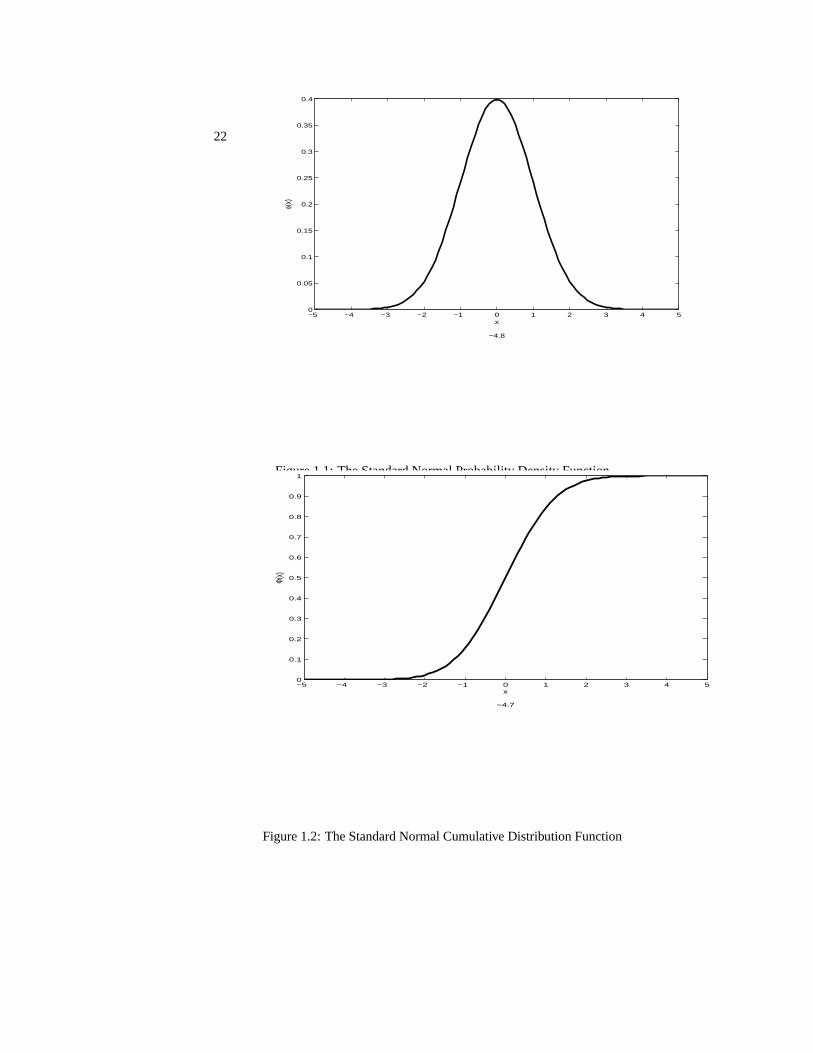
is not obtainable in simple closed form, and requires either numerical approximationor a table of values. The probability density function f(x) is symmetric about 0 andappears roughly as follows:

The integral of the standard normal probability density function is 1, but to showthis requires conversion to polar coordinates. If we square the integral of the normalprobability density function, we obtainµZ ∞−∞

1√2π

e−12y

2

dy

¶µZ ∞−∞

1√2π

e−12x

2

dx

¶=1

2π

Z ∞−∞

Z ∞−∞

e−12 (x

2+y2)dxdy

=1

2π

Z ∞0

Z 2π

0

e−12 r

2

rdθdr where x = r cos θ and y = r sin θ

= 1

22

−5 −4 −3 −2 −1 0 1 2 3 4 50

0.05

0.1

0.15

0.2

0.25

0.3

0.35

0.4

x

−4.8

φ(x)

Figure 1.1: The Standard Normal Probability Density Function

−5 −4 −3 −2 −1 0 1 2 3 4 50

0.1

0.2

0.3

0.4

0.5

0.6

0.7

0.8

0.9

1

Φ(x)

x

−4.7

Figure 1.2: The Standard Normal Cumulative Distribution Function

23

The normal cumulative distribution function is as given in Figure 1.2.We usually provide the values of the normal cumulative distribution function either

through a function such as normcdf in Matlab or through a table of values such as TableA1 (a much more compact version than that found at the back of most statistics books).

x .0 .1 .2 .3 .4 .5 .6 .7 .8 .90. .500 .540 .579 .618 .655 .692 .726 .758 .788 .8161. .841 .864 .885 .903 .919 .933 .945 .955 .964 .9712. .977 .982 .986 .989 .992 .994 .995 .997 .997 .9983. .9987 .9990 .9993 .9995 .9997 .9998 .9998 .9999 .9999 .99995

Table A1:Values of the Standard Normal Cumulative Distribution Function Φ(x)

For example we can obtainΦ(1.1) = 0.864, Φ(0.6) = 0.726,Φ(−0.5) = 1− Φ(0.5) = 1− 0.692

Note, for example that Φ(−x) = 1−Φ(x) for all x and if Z has a standard normaldistribution, we can find probabilities of intervals such as

P [−1 < Z < 1] ≈ .68 and P [−2 < Z < 2] ≈ .95.

The General Normal Distribution.

If we introduce a shift in the location in the graph of the normal density as well as achange in scale, then the resulting random variable is of the form

X = µ+ σZ,Z ∼ N(0, 1)

for some constants −∞ < µ <∞, σ > 0. In this case, since

P (X ≤ x) = P (Z ≤ x− µ

σ) = Φ(

x− µ

σ)

it is easy to show by differentiating this with respect to x that the probability densityfunction of X is

f(x;µ, σ) =1√2πσ

e−(x−µ)2/2σ2

If a random variable X has the above normal distribution with location µ and scale σwe will denote this by X ∼ N(µ, σ2).

Moments

Show that the function f(x;µ, σ) integrates to 1 and is therefore a probability densityfunction. It is not too hard to find the expected value and variance of a random variable

24

having the probability density function f(x;µ, σ) by integration:

E(X) =

Z ∞−∞

xf(x;µ, σ)dx = µ

V ar(X) =

Z ∞−∞(x− µ)2f(x;µ, σ)dx = σ2

and this gives meaning to the parameters µ and σ2, the former being the mean orexpected value of the distribution and the latter the variance.

Linear Combinations of Normal Random Variables

Suppose X1 ∼ N(µ1, σ21) and X2 ∼ N(µ2, σ

22) are independent random variables.

Then X1 + X2 ∼ N(µ1 + µ2, σ21 + σ22). More generally if we sum independent

random variables each having a normal distribution, the sum itself also has a normaldistribution. The expected value of the sum is the sum of the expected values of theindividual random variables and the variance of the sum is the sum of the variances.

Problem.

Suppose Xi ∼ N(µ, σ2) are independent random variables. What is the distribution ofthe sample mean

Xn =

Pni=1Xi

n

Assume σ = 1 and find the probability P [|Xn − µ| > 0.1] for various values of n.What happens to this probability as n→∞?

The Central Limit TheoremThe major reason that the normal distribution is the single most commonly used dis-tribution is the fact that it tends to approximate the distribution of sums of randomvariables. For example, if we throw n dice and Sn is the sum of the outcomes, whatis the distribution of Sn?. The tables below provide the number of ways in which agiven value can be obtained. The corresponding probability is obtained by dividing by6n. For example on the throw of n = 1 dice the probable outcomes are 1,2,...,6 withprobabilities all 1/6 as indicated in the histogram below:

If we sum the values on two fair dice, the possible outcomes are the values 2,3,...,12as shown in the following table and the probabilities are the values below:

Values 2 3 4 5 6 7 8 9 10 11 12Probabilities×36 1 2 3 4 5 6 5 4 3 2 1

The probability histogram of these values is also shown:Finally for the sum of the values on three independent dice, the values range from

3 to 18 and have probabilities which, when multiplied by 63 result in the values1 3 6 10 15 21 25 27 27 25 21 15 10 6 3 1

to which we can fit three separate quadratic functions one in the middle region and one

25

1 2 3 4 5 60

0.02

0.04

0.06

0.08

0.1

0.12

0.14

0.16

0.18

Figure 1.3: The sum of n = 1 discrete uniform 1,2,3,4,5,6Random Variables

2 3 4 5 6 7 8 9 10 11 120

1

2

3

4

5

6

Figure 1.4: The sum of n = 2 discrete uniform 1,2,3,4,5,6Random Variables

2 4 6 8 10 12 14 16 18 200

5

10

15

20

25

30

Figure 1.5: The distribution of the sum of three discrete Uniform 1,2,3,4,5,6 RandomVariables

26

in each of the two tails. The histogram of these values shown in Figure 1.5 alreadyresembles a normal probability density function.

In general, these distributions show a simple pattern. For n = 1, the probabilityfunction is a constant (polynomial degree 0). For n = 2, two linear functions splicedtogether. For n = 3 a spline consisting of three quadratic pieces (polynomials ofdegree n−1). In general the histogram for Sn, the sum of the values on n independentdice, consists of n piecewise polynomials of degree n − 1. These histograms rapidlyapproach the shape of the normal probability density function.

Example

Let Xi = 0 or 1 when the i0th toss of a biased coin is Tails or Heads respectively. Whatis the distribution of Sn =

Pni=1Xi ? Consider the standardized random variable

obtained by subtracting E(Sn) and dividing by its standard deviation or the squareroot of var(Sn) :

S∗n =Sn − nppnp(1− p)

Suppose we approximate the distribution of S∗nfor large values of n.First let an integer x ∼ np + z

pnp(1− p) for fixed z and 0 < p < 1. Then as

n→∞, x/n→ p. Stirling’s approximation implies thatµn

x

¶∼

√2πnn+1/2e−n

2πxx+1/2(n− x)n−x+1/2∼ 1p

2πnp(1− p)( xn )x(1− x

n)n−x .

Also using the series expansion ln(1 + x) = x − 12x

2 + O¡x3¢, putting σ =q

p(1−p)n , and noting that σ → 0 as n→∞,

ln px(1− p)n−x

( xn)x(1− x

n)n−x = x ln(

p

p+ zσ) + (n− x) ln(

1− p

1− p− zσ)

= −x ln(1 + zσ

p)− (n− x) ln(1− zσ

1− p)

= −n(p+ zσ) ln(1 +zσ

p)− n(1− p− zσ) ln(1− zσ

1− p)

= −n(p+ zσ)(zσp)− 1

2(zσ

p)2 +O(

zσ

p)3

− n(1− p− zσ)−( zσ

1− p)− 1

2(zσ

1− p)2 +O(

zσ

1− p)3

= −nzσ + z2σ2

p− 12

z2σ2

p− zσ +

z2σ2

1− p− 12

z2σ2

1− p+O(σ3)

= −12z2σ2(

n

p+

n

1− p) +O(n−1/2)

= −z2

2+O(n−1/2)

Therefore,

27

P [Sn = x] = P [S∗n = z] =

µn

x

¶px(1− p)n−x

∼µn

x

¶(x

n)x(1− x

n)n−x

px(1− p)n−x

( xn)x(1− x

n)n−x

∼ 1pnp(1− p)

1√2π

e−z2/2.

This is the standard normal probability density function multiplied by the distancebetween consecutive values of S∗n. In other words, this result says that the area underthe probability histogram for S∗n for the bar around the point z can be approximatedby the area under the normal curve between the same two points (z ± 1

2√np(1−p) ).

Theorem A8

Let Xi, i = 1, . . . n be independent random variables all with the same distribution,and with mean µ and variance σ2. Then the cumulative distribution function of

S∗n =Pn

i=1Xi − nµ√nσ

converges to the cumulative distribution function of a standard normal random vari-able.

Consider, for example, the case where theXi are independent each with a Bernoulli(p) distribution. Then the sum

Pni=1Xi has a binomial distribution with parame-

ters n, p and the above theorem asserts that if we subtract the mean and we divideby the standard deviation of a binomial random variable, then the result is approx-imately standard normal. In other words, for large values of n a binomial randomvariable is approximately normal (np, np(1− p)). To verify this fact, we plot both thebinomial(100, 0.4) histogram as well as the normal probability density function below.

Problem

Use the central limit theorem and the normal approximation to a probability histogramto estimate the probability that the sum of the numbers on 5 dice is 15. Compare youranswer with the exact probability.

The Distribution of a Function of a Random Variable.

We have seen that if X has a normal distribution, then a linear function of X, sayaX + b also has a normal distribution. The parameters are easily determined sinceE(aX + b) = aE(X) + b and var(aX + b) = a2var(X). Is this true of arbitraryfunctions and general distributions? For example is X2 normally distributed? Theanswer in general is NO. For example, the distribution of X2 must be concentratedentirely on the positive values of x, whereas the normal distributions are all supported

28

20 25 30 35 40 45 50 55 600

0.01

0.02

0.03

0.04

0.05

0.06

0.07

0.08

0.09

xf(x

)

Comparison of N(40,24) and Bin(100,.4) probs

Figure 1.6: Binomial (100, 0.4) Probability histogram together with N(40, 24) proba-bility desity function

on the whole real line (i.e. the probability density function f(x) > 0, all x ∈ R).In general, the safest method for finding the distribution of the function of a randomvariable in the continuous case is to first find the cumulative distribution of the functionand then differentiate to obtain the probability density function. This allows us to verifythe result below:

Theorem A9

Suppose a continuous random variable X has probability density function fX(x).Then the probability density function of Y = h(X) where h(.) is a continuousmonotone increasing function with inverse function h−1(y) is

fY (y) = fX(h−1(y))

d

dyh−1(y)

1.6 Moment Generating FunctionsConsider a random variable X. We have seen several ways of describing its distri-bution, using either a cumulative distribution function, a probability density function(continuous case) or probability function or a probability histogram or table (dis-crete case). We may also use some transform of the probability density or probabilityfunction. For example, consider the function defined by

MX(t) = EetX

defined for all values of t such that this expectations exists and is finite. This functionis called the moment generating function of the (distribution of the) random variable

29

X. It is a powerful tool for determining the distribution of sums of independent randomvariables and for proving the central limit theorem. In the discrete case we can writeMX(t) =

Px e

xtP [X = x] and in the continuous case MX(t) =R∞−∞ extf(x)dx.

The logarithm of the moment generating function ln(MX(t)) is called the cumulantgenerating function.

Properties of the Moment Generating Function

For these properties we assume that the moment generating function exists at least insome neighbourhood of the value t = 0, say for − < t < for some > 0. Wealso assume that d

dtE[XnetX = E[ ddtX

netX ] for each value of n = 0, 1, 2, for− < t < . The ability to differentiate under an integral or infinite sum is justifiedunder general conditions involving the rate at which the integral or series converges.

1. M 0(0) = E(X)

2. M (n)(0) = E(Xn), n = 1, 2, ...

3. A moment generating function uniquely determines a distribution. In otherwords if MX(t) = MY (t) for all − < t < , then X and Y have thesame distribution.

4. MaX+b(t) = ebtMX(at) for constants a, b.

5. If X and Y are independent random variables, MX+Y (t) =MX(t)MY (t).

Examples

Let X have a distribution as given in the table below Then the moment generatingfunction of X is:

Distribution Moment Generating Function MX(t)Binomial (n, p) (pet + 1− p)n

Poisson(λ ) expλ(et − 1)Exponential, mean µ 1

1−µt for t < 1/µNormal (µ, σ2) expµt+ σ2t2/2

Moment generating functions are useful for showing that a sequence of cumulativedistribution functions converge because of the following result. The result implies thatconvergence of the moment generating functions can be used to show convergence ofthe cumulative distribution functions ( i.e. convergence of the distributions).

Theorem A10

Suppose Zn is a sequence of random variables with moment generating functionsMn(t). Let Z be a random variable Z having moment generating function M(t).If Mn(t)→M(t) for all t in a neighbourhood of 0, then

P [Zn ≤ z]→ P [Z ≤ z]

as n→∞ for all values of z at which the function FZ(z) is continuous.

30

1.7 Joint Distributions and ConvergenceConsider constructing measures on a product Euclidean space. Given Lebesgue mea-sure λ, essentially a measure of length on the real line < how do we construct a similarmeasure, compatible with the notion of area in two-dimensional Euclidean space? Wenaturally begin with the measure of rectangles or indeed any product set of the formA × B = (x, y);x ∈ A, y ∈ B for arbitrary (Borel) sets A ⊂ <, B ⊂ <. Themeasure of a product set can be defined as the product of the measure of the two factorsets,µ(A × B) = λ(A)λ(B). This defines a measure for any product set and by anextension theorem, since the product sets form a Boolean algebra, we can extend thismeasure to the sigma algebra generated by the product sets.

More formally, suppose we are given two measure spaces (M,M, µ) and (N,N , ν) .Define the product space to be the space consisting of pairs of objects, one from eachof M and N ,

Ω =M ×N = (x, y); x ∈M, y ∈ N.The Cartesian product of two setsA ⊂M, and B ⊂ N is denotedA×B = (a, b); a ∈A, b ∈ B. This is the analogue of a rectangle, a subset of M × N , and it is easy todefine a measure for such sets as follows. Define the product measure of product setsof the above form by π(A × B) = µ(A)ν(B). The following theorem is a simpleconsequence of the Caratheodory Extension Theorem.

Theorem A11

The product measure π defined on the product sets of the form A×B;A ∈ N , B ∈Mcan be extended to a measure on the sigma algebra σA×B;A ∈ N ,B ∈M of sub-sets of M ×N .

There are two cases of product measure of importance. Consider the sigma algebraon <2 generated by the product of the Borel sigma algebras on <. This is called theBorel sigma algebra in <2. We can similarly define the Borel sigma algebra on <n.

Similarly, if we are given two probability spaces (Ω1,F1, P1) and (Ω2,F2, P2)wecan construct a product measure Q on the Cartesian product space Ω1 ×Ω2 such thatQ(A× B) = P1(A)P2(B) for all A ∈ F1, B ∈ F2.This guarantees the existence ofa product probability space in which events of the form A × Ω2 are independent ofevents of the form Ω1 ×B for A ∈ F1, B ∈ F2.

We say a sequence of random variables X1,X2, . . . is independent if the familyof sigma-algebras σ(X1), σ(X2), . . . are independent, that is for Borel sets Bn, n =1, . . . N in <, the events [Xn ∈ Bn], n = 1, ..., N form a mutually independent se-quence of events so that

P [X1 ∈ B1,X2 ∈ B2, ...,Xn ∈ Bn] = P [X1 ∈ B1]P [X2 ∈ B2]...P [Xn ∈ Bn]

. The sequence is said to be identically distributed every random variable Xn has thesame cumulative distribution function.

We have already seen the following result, but we repeat it here, if only to get theflavour of the proof.

31

If X,Y are independent integrable random variables on the same probability space,then XY is also integrable and

E(XY ) = E(X)E(Y ).

Proof. Suppose first that X and Y are both simple functions, X =P

ciIAi , Y =PdjIBj . Then X and Y are independent if and only if P (AiBj) = P (Ai)P (Bj)

for all i, j and so

E(XY ) = E[(X

ciIAi)(X

djIBj )]

=XX

cidjE(IAiIBj )

=XX

cidjP (Ai)P (Bj)

= E(X)E(Y ).

More generally suppose X,Y are non-negative random variables and consider inde-pendent simple functions Xn increasing to X and Yn increasing to Y. Then XnYn isa non-decreasing sequence with limit XY. Therefore, by the monotone convergencetheorem,

E(XnYn)→ E(XY ).

On the other hand,

E(XnYn) = E(Xn)E(Yn)→ E(X)E(Y ).

Therefore E(XY ) = E(X)E(Y ). The case of general (positive and negative randomvariables X,Y we leave as a problem.

Joint Distributions of more than 2 random variables

SupposeX1, ...,Xn are random variables defined on the same probability space (Ω,F , P )(but not necessarily independent). The joint distribution can be characterized by thejoint cumulative distribution function, a function on <n defined by

F (x1, ..., xn) = P [X1 ≤ x1, ...,Xn ≤ xn] = P ([X1 ≤ x1] ∩ .... ∩ [Xn ≤ xn]).

The joint cumulative distribution function allows us to findP [a1 < X1 ≤ b1, ..., an <Xn ≤ bn]. By the inclusion-exclusion principle,

P [a1 < X1 ≤ b1, ..., an < Xn ≤ bn] (1.8)

= F (b1, b2, . . . bn)−Xj

F (b1, ..., aj , bj+1, ...bn)

+Xi<j

F (b1, ..., ai, bi+1...aj , bj+1, ...bn)− ...

As in the case, we may then build a probability measure on an algebra of subsets of<n. This measure is then extended to the Borel sigma-algebra on <n.

32

Theorem A12

The joint cumulative distribution function has the following properties:(a) F (x1, ..., xn) is right-continuous and non-decreasing in each argument xi when

the other arguments xj , j 6= i are fixed.(b) F (x1, ..., xn) → 1 as min(x1, ..., xn) → ∞ and F (x1, ..., xn) → 0 as

min(x1, ..., xn)→ −∞.(c) The expression on the right hand side of (1.8) is greater than or equal to zero

for all a1, . . . an, b1, . . . , bn.

The joint probability distribution of the variables X1, ...,Xn is a measure on Rn.It can be determined from the cumulative distribution function in the usual fashion,first by defining the measure of intervals and then extending this to the sigma algebragenerated by these intervals. In order to verify that the random variables are mutuallyindependent, it is sufficient to verify that the joint cumulative distribution functionfactors;

F (x1, ..., xn) = F1(x1)F2(x2)...Fn(xn) = P [X1 ≤ x1] . . . P [Xn ≤ xn]

for all x1, ...., xn ∈ <.

Theorem A13

If the random variables X1, ...,Xn are mutually independent, then

E[nYj=1

gj(Xj)] =nYj=1

E[gj(Xj)]

for any Borel measurable functions g1, . . . , gn.An infinite sequence of random variables X1,X2, . . . is mutually independent if

every finite subset is mutually independent.

Definition (Strong (almost sure) Convergence)

Let X and Xn, n = 1, 2, . . . be random variables all defined on the same probabil-ity space (Ω,F). We say that the sequence Xn converges almost surely (or withprobability one) to X (denoted Xn → X a.s.) if the event

ω;Xn(ω)→ X(ω) = ∩∞m=1[|Xn −X| ≤ 1

ma.b.f.o.]

has probability one. Here the notation a.b.f.o., standing for “all but finitely often” is the“lim inf” of the events [|Xn −X| ≤ 1

m ].In order to show a sequence Xn converges almost surely, we need that Xn are

(measurable) random variables for all n, and to show that there is some measurablerandom variable X for which the set ω;Xn(ω) → X(ω) is measurable and hence

33

an event, and that the probability of this event P [Xn → X] is 1.Alternatively we canshow that for each value of > 0, P [|Xn −X| > i.o.] = 0, or in other words thatthe probability of the set of all points ω such that Xn(ω) does not converge to X(ω) iszero. It is sufficient to consider values of of the form = 1/m, m=1,2,... above.

The law of large numbers (sometimes called the law of averages) is the best-knownresult in probability. It says, for example, that the average of independent Bernoullirandom variables, or Poisson, or negative binomial, or Gamma random variables, toname a few, converge to their expected value with probability one.

Theorem A14 (Strong Law of Large Numbers)

If Xn, n = 1, 2, . . . is a sequence of independent identically distributed random vari-ables with E|Xn| <∞, (i.e. they are integrable) and E(Xn) = µ, then

1

n

nXi=1

Xi → µ almost surely as n→∞

1.8 Weak Convergence (Convergence in Distribution)Consider random variables that are constants; Xn = 1+

1n . By any sensible definition

of convergence, Xn converges to X = 1 as n → ∞. Does the cumulative distrib-ution function of Xn, Fn,say, converge to the cumulative distribution function of Xpointwise? In this case it is true that Fn(x) → F (x) at all values of x except thevalue x = 1 where the function F (x) has a discontinuity. Convergence in distribution(weak convergence, convergence in Law) is defined as pointwise convergence of thec.d.f. at all values of x except those at which F (x) is discontinuous. Of course if thelimiting distribution is absolutely continuous (for example the normal distribution as inthe Central Limit Theorem), then Fn(x)→ F (x) does hold for all values of x.

Definition (Weak Convergence)

If Fn(x), n = 1, . . . is a sequence of cumulative distribution functions and if Fis a cumulative distribution function, we say that Fn converges to F weakly orin distribution if Fn(x) → F (x) for all x at which F (x) is continuous. Weakconvergence of a sequence of random variables Xn whose c.d.f. converges in theabove sense is denoted in a variety of ways such as Xn ⇒ X or Xn →D X (here“D” stands for “in distribution”).

There are simple examples of cumulative distribution functions that converge point-wise but not to a genuine cumulative distribution because some of the mass of the dis-tribution escapes to infinity. For example if Fn is the cumulative distribution functionof a point mass at the point n then Fn(x) → 0 for each fixed value of x < ∞. Anadditional condition called tightness is needed to insure that the limiting distributionis a “proper” probability distribution (i.e. has total measure 1). A sequence of proba-bility measures Pn on Euclidean space is tight if for all > 0, there exists a boundedrectangle K such that Pn(K) > 1− for all n. A sequence of cumulative distribution

34

functions Fn is tight if, for every > 0, there is a value of M < ∞ such that theprobabilities of interval [−M,M ] are greater than than 1− ,

Fn(M)− Fn(−M) ≤ 1− for all n = 1, 2, ...

If a sequence Fn converges to some limiting right-continuous function F at continu-ity points of F and if the sequence is tight, then the limiting function F is a propercumulative distribution function and the convergence is in distribution. There is a moregeneral definition of weak convergence that is used for stochastic processes or moregeneral spaces of random elements.

Definition (general definition of weak convergence)

A sequence of random elements of a metric space Xn converges weakly to X i.e.Xn ⇒ X if and only if E[f(Xn)] → E[f(X)] for all bounded continuous functionsf .

Definition (convergence in probability)

We say a sequence of random variables Xn → X in probability if for all > 0,P [|Xn −X| > ]→ 0 as n→∞.

Convergence in probability is in general a somewhat more demanding concept thanweak convergence, but less demanding than almost sure convergence. In other words,convergence almost surely implies convergence in probability and convergence in prob-ability implies weak convergence.

Theorem A15

If Xn → X almost surely then Xn → X in probability.However, convergence in probability does not imply convergence almost surely,

but it does imply weak convergence.

Theorem A16

If Xn → X in probability, then Xn →D X.

The converse of this theorem holds under one condition, when the convergence indistribution s to a constant.

Theorem A17

If Xn →D converges in distribution to some constant c then Xn → c in probability.The next result, Fubini’s theorem, allows us to change the order of integration as

long as the function being integrated is, in fact, integrable.

35

Theorem A18 (Fubini’s Theorem)

Suppose g(x, y) is integrable with respect to a product measure π = µ×ν on M×N .Then Z

M×Ng(x, y)dπ =

ZM

[

ZN

g(x, y)dν]dµ =

ZN

[

ZM

g(x, y)dµ]dν.

Convolutions

Consider two independent random variables X, Y , both having a discrete distribution.Suppose we wish to find the probability function of the sum Z = X + Y . Then

P [Z = z] =Xx

P [X = x]P [Y = z − x] =Xx

fX(x)fY (z − x).

Similarly, if X,Y are independent absolutely continuous distributions with probabilitydensity functions fX , fY respectively, then we find the probability density function ofthe sum Z = X + Y by

fZ(z) =

Z ∞−∞

fX(x)fY (z − x)dx

In both the discrete and continuous case, we can rewrite the above in terms of thecumulative distribution function FZ of Z. In either case,

FZ(z) = E[FY (z −X)] =

Z<FY (z − x)FX(dx)

We use the last form as a more general definition of a convolution between two cu-mulative distribution functions F,G. We define the convolution of F and G to beF ∗G(x) = R∞

−∞ F (x− y)dG(y) .

Properties of convolution

(a) If F,G are cumulative distributions functions, then so is F ∗G

(b) F ∗G = G ∗ F

(c) If either F or G are absolutely continuous with respect to Lebesgue measure,then F ∗G is absolutely continuous with respect to Lebesgue measure.

The convolution of two cumulative distribution functions F ∗G represents the c.d.fof the sum of two independent random variables, one with c.d.f. F and the other withc.d.f. G.

36

1.9 Stochastic ProcessesA Stochastic process is an indexed family of random variables Xt for t ranging oversome index set T such as the integers or an interval of the real line. For examplea sequence of independent random variables is a stochastic process, as is a Markovchain. For an example of a continuous time stochastic process, define Xt to be theprice of a stock at time t (assuming trading occurs continuously over time).

Markov Chains

Consider a sequence of (discrete) random variables X1,X2, . . .each of which takes in-teger values 1, 2, . . . N (called states). We assume that for a certain matrix P (called thetransition probability matrix), the conditional probabilities are given by correspondingelements of the matrix; i.e.

P [Xn+1 = j|Xn = i] = Pij , i = 1, . . . N, j = 1, . . . N

and furthermore that the chain only cares about the last state occupied in determiningits future; i.e. that

P [Xn+1 = j|Xn = i,Xn−1 = i1,Xn−2 = i2...Xn−l = il] = P [Xn+1 = j|Xn = i] = Pij

for all j, i, i1, i2, . . . il, and l = 2, 3, .... Then the sequence of random variables Xn iscalled a Markov Chain. Markov Chain models are the most common simple modelsfor dependent variables, including weather (precipitation, temperature), movements ofsecurity prices etc. They allow the future of the process to depend on the present stateof the process, but the past behaviour can influence the future only through the present.

Properties of the Transition Matrix P

Note that Pij ≥ 0 for all i, j andP

j Pij = 1 for all i. This last property impliesthat the N ×N matrix P − I (where I is the identity matrix) has rank at most N − 1because the sum of the N columns of P − I is identically 0.

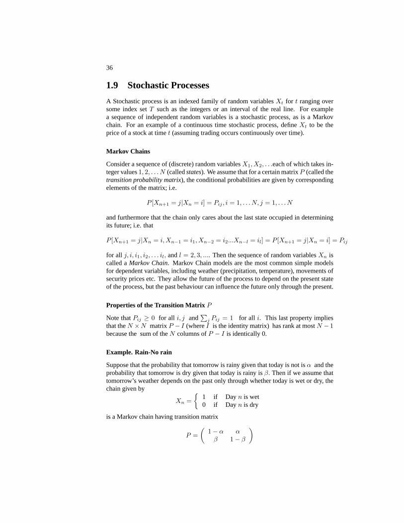
Example. Rain-No rain

Suppose that the probability that tomorrow is rainy given that today is not is α and theprobability that tomorrow is dry given that today is rainy is β. Then if we assume thattomorrow’s weather depends on the past only through whether today is wet or dry, thechain given by

Xn =

½1 if Day n is wet0 if Day n is dry

is a Markov chain having transition matrix

P =

µ1− α αβ 1− β

¶

37

The distribution of Xn

Suppose that the chain is started by randomly choosing a state for X0 with distributionP [X0 = i] = qi, i = 1, 2, . . . N . Then the distribution of X1 is given by

P (X1 = j) =NXi=1

P (X1 = j,X0 = i)

=NXi=1

P (X1 = j|X0 = i)P (X0 = i)

=NXi=1

Pijqi

and this is the j0th element of the vector q0P where q is the column vector of valuesqi. Similarly the distribution of Xn is the vector q0Pn where Pn is the product of thematrix P with itself n times. Under very general conditions, it can be shown that theseprobabilities converge and in many such cases, the limit does not depend on the initialdistribution q.

Definition

A limiting distribution of a Markov chain is a vector (π say) of long run probabilitiesof the individual states so

πi = limt→∞P [Xt = i].

Definition

A stationary distribution of a Markov chain is the column vector (π say) of probabili-ties of the individual states such that

π0P = π0.

Theorem A19

Any limiting distribution of a Markov Chain must be a stationary distribution.Proof.Note that π0 = limn→∞ q0Pn = limn→∞(q0Pn)P = (limn→∞ q0Pn)P = π0P.

Example: Binary information:

Suppose that X1,X2, . . . is a sequence of binary information (Bernoulli random vari-ables) taking values either 0 or 1. Suppose that the probability that a 0 is followed by a1 is p and the probability that a 1 is followed by a 0 is given by q where 0 < p, q < 1.Then the transition matrix for the Markov chain is

P =

µ1− p pq 1− q

¶

38

The limiting distribution for this Markov Chain is

π =

µ qp+qp

p+q

¶so, for example, the long run proportion of zeros in the sequence is q

p+q .When is the limiting distribution of a Markov chain unique and independent of the

initial state of the chain?

Definition: irreducible, aperiodic

We say that a Markov chain is irreducible if every state can be reached from everyother state. In other words for every pair i, j there is some m such that P (m)i,j > 0. Wesay that the chain is aperiodic if, for each state i, there is no regular or periodic patternfor the values of k for which P

(k)ii > 0. For example if P (1)ii = 0, P

(2)ii > 0, P

(3)ii =

0, P(4)ii > 0 and this pattern continues indefinitely then the greatest common divisor

of the values k such that P (N)ii > 0 is evidently 2. We write this mathematically asgcdk;P (k)ii > 0 = 2 and this chain is not aperiodic, it has period 2. On the other handif for all states i, gcdk;P (k)ii > 0 = 1, we say the chain is aperiodic. For a periodicchain (i.e. one that is not aperiodic, so the period gcdk;P (k)ii > 0 is greater thanone) returns to a state can occur only at multiples of the period gcdN ;P (N)ii > 0.

Theorem A20

If a Markov chain is irreducible and aperiodic, then there exists a unique limiting distri-bution π. In this case, as n→∞, Pn → π01

¯the matrix whose rows are all identically

π0.

Generating FunctionsDefinition: Generating function

Let a0, a1, a2, . . . be a finite or infinite sequence of real numbers. Suppose the powerseries

A(t) =∞Xi=0

aiti

converges for all − < t < for some value of > 0. Then we say that the sequencehas a generating function A(t).

Note. Every bounded sequence has a generating function since the seriesP∞

i=0 ti

converges whenever |t| < 1. Thus, discrete probability functions have generatingfunctions. The generating function of a random variable X or its associated probabilityfunction fX(x) = P [X = x] is given by

FX(t) =Xx

fX(x)tx = E(tX).

39

Note that if the random variable has finite expected value, then this converges on theinterval t ∈ [−1, 1].

The advantage of generating functions is that they provide a transform of the origi-nal distribution to a space where many operations are made much easier. We will giveexamples of this later. The most important single property is that they are in one-onecorrespondence with distributions such that the series converges; for each distributionthere is a unique generating function and for each generating function there is a uniquedistribution.

As a consequence of this representation and the following theorem we can use gen-erating functions to determine distributions that would otherwise be difficult to identify.

Theorem A21

Suppose a random variable X has generating function FX(t) and Y has generatingfunction FY (t). Suppose that X and Y are independent. Then the generating functionof the random variable W = X + Y is FW (t) = FX(t)FY (t).

Notice that whenever a moment generating function exists, we can recover thegenerating function from it by replacing et by t.

Example

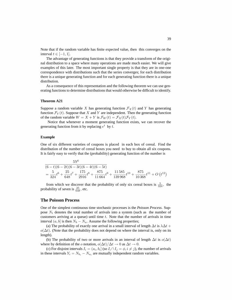
One of six different varieties of coupons is placed in each box of cereal. Find thedistribution of the number of cereal boxes you need to buy to obtain all six coupons.It is fairly easy to verify that the (probability) generating function of the number is

5!t6

(6− t)(6− 2t)(6− 3t)(6− 4t)(6− 5t)=

5

324t6 +

25

648t7 +

175

2916t8 +

875

11 664t9 +

11 585

139 968t10 +

875

10 368t11 +O

¡t12¢

from which we discover that the probability of only six cereal boxes is 5324 , the

probability of seven is 25648 , etc.

The Poisson ProcessOne of the simplest continuous time stochastic processes is the Poisson Process. Sup-pose Nt denotes the total number of arrivals into a system (such as the number ofcustomers arriving at a queue) until time t. Note that the number of arrivals in timeinterval (a, b] is then Nb −Na. Assume the following properties;

(a) The probability of exactly one arrival in a small interval of length ∆t is λ∆t+o(∆t). (Note that the probability does not depend on where the interval is, only on itslength).

(b) The probability of two or more arrivals in an interval of length ∆t is o(∆t)where by definition of the o notation, o(∆t)/∆t→ 0 as∆t→ 0.

(c) For disjoint intervals Ii = (ai, bi] (so Ii∩ Ij = φ, i 6= j), the number of arrivalsin these intervals Yi = Nbi −Nai are mutually independent random variables.

40

Theorem A22

Under the above conditions, (a)-(c), the distribution of the process Nt, t ∈ T is that ofa Poisson process. This means that the number of arrivals Nb−Na in an interval (a, b]has a Poisson distribution with parameter λ(b− a) = λ×the length of the interval, andthe number of arrivals in disjoint time intervals are independent random variables. Theparameter λ specifies the rate of the Poisson process.

We can easily show that if N(t) is a Poisson process and T1, T2, .... are the timesof the first event, and the time between the first and second events, etc. then T1, T2, ...are independent random variables, each with an exponential distribution with expectedvalue 1/λ. Moreover if T1, T2, ... Tn are independent random variables each with anexponential (1) distribution, then the sum

Pni=1 Ti has a (gamma) probability density

function with probability density function

f(x) =1

(n− 1)!xn−1e−x, for x > 0.

This means that the event times for a Poisson process are Gamma distributed.

Poisson Process in space.

In an analogous way we may define a Poisson process in space as a distribution govern-ing the occurrence of random points with the properties indicated above; The numberof points in a given set S has a Poisson distribution with parameter λ× |S| where |S|is the area or volume of the set, and if Y1, Y2, ...are the number of points occurring indisjoint sets S1, S2, . . ., they are mutually independent random variables.