basic linear algebra - ufrgs - engenharia de produção ... · basic linear algebra ... the...

� � � � � � � � � � �

Basic Linear Algebra

In this chapter, we study the topics in linear algebra that will be needed in the rest of the book.We begin by discussing the building blocks of linear algebra: matrices and vectors. Then weuse our knowledge of matrices and vectors to develop a systematic procedure (the Gauss–Jordan method) for solving linear equations, which we then use to invert matrices. We closethe chapter with an introduction to determinants.

The material covered in this chapter will be used in our study of linear and nonlinear programming.

2.1 Matrices and VectorsMatrices

D E F I N I T I O N ■ A matrix is any rectangular array of numbers. ■

For example,

� �, � �, � �, [2 1]

are all matrices.If a matrix A has m rows and n columns, we call A an m � n matrix. We refer to

m � n as the order of the matrix. A typical m � n matrix A may be written as

A � � �D E F I N I T I O N ■ The number in the ith row and jth column of A is called the ijth element of A

and is written aij. ■

For example, if

A � � �then a11 � 1, a23 � 6, and a31 � 7.

3

6

9

2

5

8

1

4

7

a1n

a2n

��amn

��

��

��

a12

a22

��am2

a11

a21

��am1

1

�2

3

6

2

5

1

4

2

4

1

3

Sometimes we will use the notation A � [aij] to indicate that A is the matrix whoseijth element is aij.

D E F I N I T I O N ■ Two matrices A � [aij] and B � [bij] are equal if and only if A and B are of thesame order and for all i and j, aij � bij. ■

For example, if

A � � � and B � � �then A � B if and only if x � 1, y � 2, w � 3, and z � 4.

Vectors

Any matrix with only one column (that is, any m � 1 matrix) may be thought of as a columnvector. The number of rows in a column vector is the dimension of the column vector. Thus,

� �may be thought of as a 2 � 1 matrix or a two-dimensional column vector. Rm will denotethe set of all m-dimensional column vectors.

In analogous fashion, we can think of any vector with only one row (a 1 � n matrix asa row vector. The dimension of a row vector is the number of columns in the vector. Thus,[9 2 3] may be viewed as a 1 � 3 matrix or a three-dimensional row vector. In this book,vectors appear in boldface type: for instance, vector v. An m-dimensional vector (either rowor column) in which all elements equal zero is called a zero vector (written 0). Thus,

[0 0] and � �are two-dimensional zero vectors.

Any m-dimensional vector corresponds to a directed line segment in the m-dimensionalplane. For example, in the two-dimensional plane, the vector

u � � �corresponds to the line segment joining the point

� �to the point

� �The directed line segments corresponding to

u � � �, v � � �, w � � �are drawn in Figure 1.

�1

�2

1

�3

1

2

1

2

0

0

1

2

0

0

1

2

y

z

x

w

2

4

1

3

12 C H A P T E R 2 Basic Linear Algebra

The Scalar Product of Two Vectors

An important result of multiplying two vectors is the scalar product. To define the scalar prod-uct of two vectors, suppose we have a row vector u = [u1 u2 �� un] and a column vector

v � � �of the same dimension. The scalar product of u and v (written u � v) is the number u1v1 � u2v2 � �� unvn.

For the scalar product of two vectors to be defined, the first vector must be a row vec-tor and the second vector must be a column vector. For example, if

u � [1 2 3] and v � � �then u � v � 1(2) � 2(1) � 3(2) � 10. By these rules for computing a scalar product, if

u � � � and v � [2 3]

then u � v is not defined. Also, if

u � [1 2 3] and v � � �then u � v is not defined because the vectors are of two different dimensions.

Note that two vectors are perpendicular if and only if their scalar product equals 0.Thus, the vectors [1 �1] and [1 1] are perpendicular.

We note that u � v � �u� �v� cos u, where �u� is the length of the vector u and u is theangle between the vectors u and v.

3

4

1

2

2

1

2

v1

v2

��vn

2 . 1 Matrices and Vectors 13

3

2

x2

x1

1

– 1

– 2

– 2

w

u

v

– 1

(–1, –2)

(1, 2)

u =12

v =

w =

(1, –3)

1 2

– 3

1–3

–2–1

F I G U R E 1Vectors Are Directed

Line Segments

Matrix Operations

We now describe the arithmetic operations on matrices that are used later in this book.

The Scalar Multiple of a Matrix

Given any matrix A and any number c (a number is sometimes referred to as a scalar),the matrix cA is obtained from the matrix A by multiplying each element of A by c. Forexample,

if A � � �, then 3A � � �For c � �1, scalar multiplication of the matrix A is sometimes written as �A.

Addition of Two Matrices

Let A � [aij] and B � [bij] be two matrices with the same order (say, m � n). Then thematrix C � A � B is defined to be the m � n matrix whose ijth element is aij � bij. Thus,to obtain the sum of two matrices A and B, we add the corresponding elements of A andB. For example, if

A � � � and B � � �then

A � B � � � � � �.

This rule for matrix addition may be used to add vectors of the same dimension. For ex-ample, if u � [1 2] and v � [2 1], then u � v � [1 � 2 2 � 1] � [3 3]. Vectorsmay be added geometrically by the parallelogram law (see Figure 2).

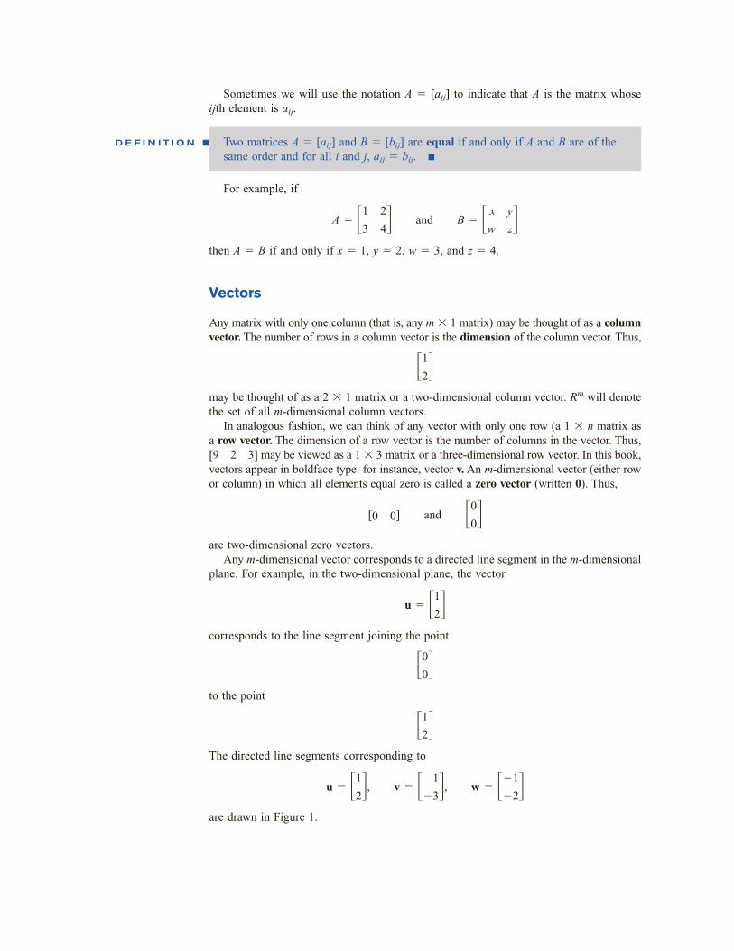
We can use scalar multiplication and the addition of matrices to define the concept of a line segment. A glance at Figure 1 should convince you that any point u in the m-dimensional plane corresponds to the m-dimensional vector u formed by joining theorigin to the point u. For any two points u and v in the m-dimensional plane, the line segment joining u and v (called the line segment uv) is the set of all points in the m-dimensional plane that correspond to the vectors cu � (1 � c)v, where 0 � c � 1 (Figure 3). For example, if u � (1, 2) and v � (2, 1), then the line segment uv consists

0

0

0

0

0

2

3 � 3

1 � 1

2 � 2

�1 � 1

1 � 1

0 � 2

�3

�1

�2

1

�1

2

3

1

2

�1

1

0

6

0

3

�3

2

0

1

�1


3

2

x2

x1

1

uu + v

v

(1, 2)

(2, 1)

(3, 3)

(0, 0)

v = 2 1

1 2 3

u = 1 2u + v = 3 3

F I G U R E 2Addition of Vectors

of the points corresponding to the vectors c[1 2] � (1 � c)[2 1] � [2 � c 1 � c],where 0 � c � 1. For c � 0 and c � 1, we obtain the endpoints of the line segment uv;for c � �

12

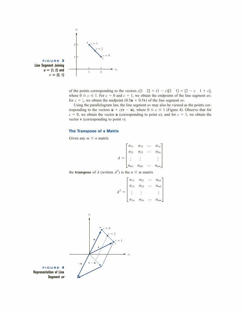
�, we obtain the midpoint (0.5u � 0.5v) of the line segment uv.Using the parallelogram law, the line segment uv may also be viewed as the points cor-

responding to the vectors u � c(v � u), where 0 � c � 1 (Figure 4). Observe that for c � 0, we obtain the vector u (corresponding to point u), and for c � 1, we obtain thevector v (corresponding to point v).

The Transpose of a Matrix

Given any m � n matrix

A � � �the transpose of A (written AT) is the n � m matrix

AT � � �am1

am2

��amn

��

��

��

a21

a22

��a2n

a11

a12

��a1n

a1n

a2n

��amn

��

��

��

a12

a22

��am2

a11

a21

��am1


2

x2

u c = 1

c = 0

c =

v

x1

1

1 2

12

F I G U R E 3Line Segment Joining

u � (1, 2) and v � (2, 1)

x2

u

u

– u v – u

v

c = 0

c = 1

c =

v

x1

12

F I G U R E 4Representation of Line

Segment uv

Thus, AT is obtained from A by letting row 1 of A be column 1 of AT, letting row 2 of Abe column 2 of AT, and so on. For example,

if A � � �, then AT � � �Observe that (AT)T � A. Let B � [1 2]; then

BT � � � and (BT)T � [1 2] � B

As indicated by these two examples, for any matrix A, (AT)T � A.

Matrix Multiplication

Given two matrices A and B, the matrix product of A and B (written AB) is defined if andonly if

Number of columns in A � number of rows in B (1)

For the moment, assume that for some positive integer r, A has r columns and B has rrows. Then for some m and n, A is an m � r matrix and B is an r � n matrix.

D E F I N I T I O N ■ The matrix product C � AB of A and B is the m � n matrix C whose ijthelement is determined as follows:

ijth element of C � scalar product of row i of A � column j of B ■ (2)

If Equation (1) is satisfied, then each row of A and each column of B will have thesame number of elements. Also, if (1) is satisfied, then the scalar product in Equation (2)will be defined. The product matrix C � AB will have the same number of rows as A andthe same number of columns as B.

Compute C � AB for

A � � � and B � � �Solution Because A is a 2 � 3 matrix and B is a 3 � 2 matrix, AB is defined, and C will be a

2 � 2 matrix. From Equation (2),

c11 � [1 1 2] � � � 1(1) � 1(2) � 2(1) � 5

c12 � [1 1 2] � � � 1(1) � 1(3) � 2(2) � 8

c21 � [2 1 3] � � � 2(1) � 1(2) � 3(1) � 7

1

2

1

1

3

2

1

2

1

1

3

2

1

2

1

2

3

1

1

1

2

1

2

4

5

6

1

2

3

3

6

2

5

1

4


Matrix MultiplicationE X A M P L E 1

c22 � [2 1 3] � � � 2(1) � 1(3) � 3(2) � 11

C � AB � � �

Find AB for

A � � � and B � [1 2]

Solution Because A has one column and B has one row, C � AB will exist. From Equation (2), weknow that C is a 2 � 2 matrix with

c11 � 3(1) � 3 c21 � 4(1) � 4

c12 � 3(2) � 6 c22 � 4(2) � 8

Thus,

C � � �

Compute D � BA for the A and B of Example 2.

Solution In this case, D will be a 1 � 1 matrix (or a scalar). From Equation (2),

d11 � [1 2]� � � 1(3) � 2(4) � 11

Thus, D � [11]. In this example, matrix multiplication is equivalent to scalar multiplica-tion of a row and column vector.

Recall that if you multiply two real numbers a and b, then ab � ba. This is called thecommutative property of multiplication. Examples 2 and 3 show that for matrix multipli-cation, it may be that AB BA. Matrix multiplication is not necessarily commutative. (Insome cases, however, AB � BA will hold.)

Show that AB is undefined if

A � � � and B � � �Solution This follows because A has two columns and B has three rows. Thus, Equation (1) is not

satisfied.

1

1

2

1

0

1

2

4

1

3

3

4

6

8

3

4

3

4

8

11

5

7

1

3

2


Row Vector Times Column VectorE X A M P L E 3

Undefined Matrix ProductE X A M P L E 4

Column Vector Times Row VectorE X A M P L E 2

Many computations that commonly occur in operations research (and other branchesof mathematics) can be concisely expressed by using matrix multiplication.To illustratethis, suppose an oil company manufactures three types of gasoline: premium unleaded,regular unleaded, and regular leaded. These gasolines are produced by mixing two typesof crude oil: crude oil 1 and crude oil 2. The number of gallons of crude oil required tomanufacture 1 gallon of gasoline is given in Table 1.

From this information, we can find the amount of each type of crude oil needed tomanufacture a given amount of gasoline. For example, if the company wants to produce10 gallons of premium unleaded, 6 gallons of regular unleaded, and 5 gallons of regularleaded, then the company’s crude oil requirements would be

Crude 1 required � (�34

�) (10) � (�23

�) (6) � (�14

�) 5 � 12.75 gallons

Crude 2 required � (�14

�) (10) � (�13

�) (6) � (�34

�) 5 � 8.25 gallons

More generally, we define

pU � gallons of premium unleaded produced

rU � gallons of regular unleaded produced

rL � gallons of regular leaded produced

c1 � gallons of crude 1 required

c2 � gallons of crude 2 required

Then the relationship between these variables may be expressed by

c1 � (�34

�) pU � (�23

�) rU � (�14

�) rL

c2 � (�14

�) pU � (�13

�) rU � (�34

�) rL

Using matrix multiplication, these relationships may be expressed by

� � � � � � �Properties of Matrix Multiplication

To close this section, we discuss some important properties of matrix multiplication. Inwhat follows, we assume that all matrix products are defined.

1 Row i of AB � (row i of A)B. To illustrate this property, let

A � � � and B � � �Then row 2 of the 2 � 2 matrix AB is equal to

1

3

2

1

2

1

2

3

1

1

1

2

pU

rU

rL

�14

�

�34

�

�23

�

�13

�

�34

�

�14

�

c1

c2


TA B L E 1Gallons of Crude Oil Required to Produce 1 Gallon of Gasoline

Crude Premium Regular RegularOil Unleaded Unleaded Leaded

1 �34

� �23

� �14

�

2 �14

� �13

� �34

�

[2 1 3] � � � [7 11]

This answer agrees with Example 1.

2 Column j of AB � A(column j of B). Thus, for A and B as given, the first column of AB is

� � � � � � �Properties 1 and 2 are helpful when you need to compute only part of the matrix AB.

3 Matrix multiplication is associative. That is, A(BC) � (AB)C. To illustrate, let

A � [1 2], B � � �, C � � �Then AB � [10 13] and (AB)C � 10(2) � 13(1) � [33].

On the other hand,

BC � � �so A(BC) � 1(7) � 2(13) � [33]. In this case, A(BC) � (AB)C does hold.

4 Matrix multiplication is distributive. That is, A(B � C) � AB � AC and (B � C)D �BD � CD.

Matrix Multiplication with Excel

Using the Excel MMULT function, it is easy to multiply matrices. To illustrate, let’s useExcel to find the matrix product AB that we found in Example 1 (see Figure 5 and fileMmult.xls). We proceed as follows:

Step 1 Enter A and B in D2:F3 and D5:E7, respectively.

Step 2 Select the range (D9:E10) in which the product AB will be computed.

Step 3 In the upper left-hand corner (D9) of the selected range, type the formula

� MMULT(D2:F3,D5:E7)

Then hit Control Shift Enter (not just Enter), and the desired matrix product will becomputed. Note that MMULT is an array function and not an ordinary spreadsheet func-tion. This explains why we must preselect the range for AB and use Control Shift Enter.

7

13

2

1

3

5

2

4

5

7

1

2

1

2

3

1

1

1

2

1

3

2

1

2

1


123456789

1011

A B C D E FMatrixMultiplication

1 1 2A 2 1 3

B 1 12 31 2

5 8C 7 11

F I G U R E 5

Mmult.xls

2.2 Matrices and Systems of Linear EquationsConsider a system of linear equations given by

a11x1 � a12x2 � �� a1nxn � b1

a21x1 � a22x2 � �� a2nxn � b2

� � � (3)� � ��

am1x1 � am2x2 � �� amnxn � bm

In Equation (3), x1, x2, . . . , xn are referred to as variables, or unknowns, and the aij’sand bi’s are constants. A set of equations such as (3) is called a linear system of m equa-tions in n variables.

D E F I N I T I O N ■ A solution to a linear system of m equations in n unknowns is a set of values forthe unknowns that satisfies each of the system’s m equations. ■

To understand linear programming, we need to know a great deal about the propertiesof solutions to linear equation systems. With this in mind, we will devote much effort tostudying such systems.

We denote a possible solution to Equation (3) by an n-dimensional column vector x,in which the ith element of x is the value of xi. The following example illustrates the con-cept of a solution to a linear system.


1 For A � � � and B � � �, find:

a �A b 3A c A � 2Bd AT e BT f ABg BA

2 Only three brands of beer (beer 1, beer 2, and beer 3)are available for sale in Metropolis. From time to time,people try one or another of these brands. Suppose that atthe beginning of each month, people change the beer theyare drinking according to the following rules:

30% of the people who prefer beer 1 switch to beer 2.20% of the people who prefer beer 1 switch to beer 3.30% of the people who prefer beer 2 switch to beer 3.30% of the people who prefer beer 3 switch to beer 2.10% of the people who prefer beer 3 switch to beer 1.For i � 1, 2, 3, let xi be the number who prefer beer i at

the beginning of this month and yi be the number who pre-fer beer i at the beginning of next month. Use matrix mul-tiplication to relate the following:

� � � �x1

x2

x3

y1

y2

y3

2�1

2

101

369

258

147

P R O B L E M SGroup A Group B

3 Prove that matrix multiplication is associative.

4 Show that for any two matrices A and B, (AB)T � BT AT.

5 An n � n matrix A is symmetric if A � AT.a Show that for any n � n matrix, AAT is a symmet-ric matrix.b Show that for any n � n matrix A, (A � AT) is asymmetric matrix.

6 Suppose that A and B are both n � n matrices. Showthat computing the matrix product AB requires n3

multiplications and n3 � n2 additions.

7 The trace of a matrix is the sum of its diagonalelements.

a For any two matrices A and B, show that trace (A � B) � trace A � trace B.b For any two matrices A and B for which the productsAB and BA are defined, show that trace AB � trace BA.

Show that

x � � �is a solution to the linear system

x1 � 2x2 � 5(4)

2x1 � x2 � 0

and that

x � � �is not a solution to linear system (4).

Solution To show that

x � � �is a solution to Equation (4), we substitute x1 � 1 and x2 � 2 in both equations and checkthat they are satisfied: 1 � 2(2) � 5 and 2(1) � 2 � 0.

The vector

x � � �is not a solution to (4), because x1 � 3 and x2 � 1 fail to satisfy 2x1 � x2 � 0.

Using matrices can greatly simplify the statement and solution of a system of linearequations. To show how matrices can be used to compactly represent Equation (3), let

A � � �, x � � �, b � � �Then (3) may be written as

Ax � b (5)

Observe that both sides of Equation (5) will be m � 1 matrices (or m � 1 column vec-tors). For the matrix Ax to equal the matrix b (or for the vector Ax to equal the vector b),their corresponding elements must be equal. The first element of Ax is the scalar productof row 1 of A with x. This may be written as

[a11 a12 �� a1n] � � � a11x1 � a12x2 � �� a1nxn

This must equal the first element of b (which is b1). Thus, (5) implies that a11x1 �a12x2 � �� a1nxn � b1. This is the first equation of (3). Similarly, (5) implies that the scalar

x1

x2

��xn

b1

b2

��bm

x1

x2

��xn

a1n

a2n

��amn

��

��

��

a12

a22

��am2

a11

a21

��am1

3

1

1

2

3

1

1

2

2 . 2 Matrices and Systems of Linear Equations 21

Solution to Linear SystemE X A M P L E 5

product of row i of A with x must equal bi, and this is just the ith equation of (3). Our dis-cussion shows that (3) and (5) are two different ways of writing the same linear system. Wecall (5) the matrix representation of (3). For example, the matrix representation of (4) is

� � � � � � �Sometimes we abbreviate (5) by writing

A�b (6)

If A is an m � n matrix, it is assumed that the variables in (6) are x1, x2, . . . , xn. Then(6) is still another representation of (3). For instance, the matrix

� � �represents the system of equations

x1 � 2x2 � 3x3 � 2

x2 � 2x3 � 3

x1 � x2 � x3 � 1

P R O B L E MGroup A

2

3

1

3

2

1

2

1

1

1

0

1

5

0

x1

x2

2

�1

1

2


2.3 The Gauss–Jordan Method for Solving Systems of Linear EquationsWe develop in this section an efficient method (the Gauss–Jordan method) for solving asystem of linear equations. Using the Gauss–Jordan method, we show that any system oflinear equations must satisfy one of the following three cases:

Case 1 The system has no solution.

Case 2 The system has a unique solution.

Case 3 The system has an infinite number of solutions.

The Gauss–Jordan method is also important because many of the manipulations used inthis method are used when solving linear programming problems by the simplex algo-rithm (see Chapter 4).

Elementary Row Operations

Before studying the Gauss–Jordan method, we need to define the concept of an elemen-tary row operation (ERO). An ERO transforms a given matrix A into a new matrix Avia one of the following operations.

1 Use matrices to represent the following system ofequations in two different ways:

x1 � x2 � 42x1 � x2 � 6x1 � 3x2 � 8

Type 1 ERO

A is obtained by multiplying any row of A by a nonzero scalar. For example, if

A � � �then a Type 1 ERO that multiplies row 2 of A by 3 would yield

A � � �Type 2 ERO

Begin by multiplying any row of A (say, row i) by a nonzero scalar c. For some j i, letrow j of A � c(row i of A) � row j of A, and let the other rows of A be the same as therows of A.

For example, we might multiply row 2 of A by 4 and replace row 3 of A by 4(row 2of A) � row 3 of A. Then row 3 of A becomes

4 [1 3 5 6] � [0 1 2 3] � [4 13 22 27]

and

A � � �Type 3 ERO

Interchange any two rows of A. For instance, if we interchange rows 1 and 3 of A, we obtain

A � � �Type 1 and Type 2 EROs formalize the operations used to solve a linear equation sys-

tem. To solve the system of equations

x1 � x2 � 2(7)

2x1 � 4x2 � 7

we might proceed as follows. First replace the second equation in (7) by �2(first equa-tion in (7)) � second equation in (7). This yields the following linear system:

x1 � x2 � 2(7.1)

2x2 � 3

Then multiply the second equation in (7.1) by �12

�, yielding the system

x1 � x2 � 2(7.2)

x2 � �32

�

Finally, replace the first equation in (7.2) by �1[second equation in (7.2)] � first equa-tion in (7.2). This yields the system

3

6

4

2

5

3

1

3

2

0

1

1

4

6

27

3

5

22

2

3

13

1

1

4

4

18

3

3

15

2

2

9

1

1

3

0

4

6

3

3

5

2

2

3

1

1

1

0

2 . 3 The Gauss–Jordan Method for Solving Systems of Linear Equations 23

x1 � �12

�(7.3)

x2 � �32

�

System (7.3) has the unique solution x1 � �12

� and x2 � �32

�. The systems (7), (7.1), (7.2),and (7.3) are equivalent in that they have the same set of solutions. This means that x1 ��12

� and x2 � �32

� is also the unique solution to the original system, (7).If we view (7) in the augmented matrix form (A�b), we see that the steps used to solve

(7) may be seen as Type 1 and Type 2 EROs applied to A�b. Begin with the augmentedmatrix version of (7):

� � � (7)

Now perform a Type 2 ERO by replacing row 2 of (7) by �2(row 1 of (7)) � row 2 of(7). The result is

� � � (7.1)

which corresponds to (7.1). Next, we multiply row 2 of (7.1) by �12

� (a Type 1 ERO), re-sulting in

� � � (7.2)

which corresponds to (7.2). Finally, perform a Type 2 ERO by replacing row 1 of (7.2)by �1(row 2 of (7.2)) � row 1 of (7.2). The result is

� � � (7.3)

which corresponds to (7.3). Translating (7.3) back into a linear system, we obtain the sys-tem x1 � �

12

� and x2 � �32

�, which is identical to (7.3).

Finding a Solution by the Gauss–Jordan Method

The discussion in the previous section indicates that if the matrix A�b is obtained fromA�b via an ERO, the systems Ax � b and Ax � b are equivalent. Thus, any sequence ofEROs performed on the augmented matrix A�b corresponding to the system Ax � b willyield an equivalent linear system.

The Gauss–Jordan method solves a linear equation system by utilizing EROs in a system-atic fashion. We illustrate the method by finding the solution to the following linear system:

2x1 � 2x2 � 2x3 � 9

2x1 � 2x2 � 2x3 � 6 (8)

x1 � 2x2 � 2x3 � 5

The augmented matrix representation is

A�b � � � � (8)

Suppose that by performing a sequence of EROs on (8) we could transform (8) into

9

6

5

1

2

2

2

�1

�1

2

2

1

�12

�

�32

�

0

1

1

0

2

�32

�

1

1

1

0

2

3

1

2

1

0

2

7

1

4

1

2


� � � (9)

We note that the result obtained by performing an ERO on a system of equations canalso be obtained by multiplying both sides of the matrix representation of the system ofequations by a particular matrix. This explains why EROs do not change the set of solu-tions to a system of equations.

Matrix (9) corresponds to the following linear system:

x1 � 1

x2 � 2 (9)

x3 � 3

System (9) has the unique solution x1 � 1, x2 � 2, x3 � 3. Because (9) was obtainedfrom (8) by a sequence of EROs, we know that (8) and (9) are equivalent linear systems.Thus, x1 � 1, x2 � 2, x3 � 3 must also be the unique solution to (8). We now show howwe can use EROs to transform a relatively complicated system such as (8) into a relativelysimple system like (9). This is the essence of the Gauss–Jordan method.

We begin by using EROs to transform the first column of (8) into

� �Then we use EROs to transform the second column of the resulting matrix into

� �Finally, we use EROs to transform the third column of the resulting matrix into

� �As a final result, we will have obtained (9). We now use the Gauss–Jordan method tosolve (8). We begin by using a Type 1 ERO to change the element of (8) in the first rowand first column into a 1. Then we add multiples of row 1 to row 2 and then to row 3(these are Type 2 EROs). The purpose of these Type 2 EROs is to put zeros in the rest ofthe first column. The following sequence of EROs will accomplish these goals.

Step 1 Multiply row 1 of (8) by �12

�. This Type 1 ERO yields

A1�b1 � � � �Step 2 Replace row 2 of A1�b1 by �2(row 1 of A1�b1) � row 2 of A1�b1. The result ofthis Type 2 ERO is

A2�b2 � � � ��92

�

�3

5

�12

�

1

2

1

�3

�1

1

0

1

�92

�

6

5

�12

�

2

2

1

�1

�1

1

2

1

0

0

1

0

1

0

1

0

0

1

2

3

0

0

1

0

1

0

1

0

0


Step 3 Replace row 3 of A2�b2 by �1(row 1 of A2�b2 � row 3 of A2�b2. The result of thisType 2 ERO is

A3�b3 � � � �The first column of (8) has now been transformed into

� �By our procedure, we have made sure that the variable x1 occurs in only a single equation

and in that equation has a coefficient of 1. We now transform the second column of A3�b3 into

� �We begin by using a Type 1 ERO to create a 1 in row 2 and column 2 of A3�b3. Then weuse the resulting row 2 to perform the Type 2 EROs that are needed to put zeros in therest of column 2. Steps 4–6 accomplish these goals.

Step 4 Multiply row 2 of A3�b3 by ��13

�.The result of this Type 1 ERO is

A4�b4 � � � �Step 5 Replace row 1 of A4�b4 by �1(row 2 of A4�b4) � row 1 of A4�b4. The result ofthis Type 2 ERO is

A5�b5 � � � �Step 6 Replace row 3 of A5�b5 by 2(row 2 of A5�b5) � row 3 of A5�b5. The result of thisType 2 ERO is

A6�b6 � � � �Column 2 has now been transformed into

� �Observe that our transformation of column 2 did not change column 1.

To complete the Gauss–Jordan procedure, we must transform the third column of A6�b6 into

� �0

0

1

0

1

0

�72

�

1

�52

�

�56

�

��13

�

�56

�

0

1

0

1

0

0

�72

�

1

�12

�

�56

�

��13

�

�32

�

0

1

�2

1

0

0

�92

�

1

�12

�

�12

�

��13

�

�32

�

1

1

�2

1

0

0

0

1

0

1

0

0

�92

�

�3

�12

�

�12

�

1

�32

�

1

�3

�2

1

0

0


We first use a Type 1 ERO to create a 1 in the third row and third column of A6�b6. Thenwe use Type 2 EROs to put zeros in the rest of column 3. Steps 7–9 accomplish thesegoals.

Step 7 Multiply row 3 of A6�b6 by �65

�. The result of this Type 1 ERO is

A7�b7 � � � �Step 8 Replace row 1 of A7�b7 by ��

56

�(row 3 of A7�b7) � row 1 of A7�b7. The result ofthis Type 2 ERO is

A8�b8 � � � �Step 9 Replace row 2 of A8�b8 by �

13

�(row 3 of A8�b8) � row 2 of A8�b8. The result of thisType 2 ERO is

A9�b9 � � � �A9�b9 represents the system of equations

x1x2x3 � 1

x1x2x3 � 2 (9)

x1x2x3 � 3

Thus, (9) has the unique solution x1 � 1, x2 � 2, x3 � 3. Because (9) was obtained from(8) via EROs, the unique solution to (8) must also be x1 � 1, x2 � 2, x3 � 3.

The reader might be wondering why we defined Type 3 EROs (interchanging of rows).To see why a Type 3 ERO might be useful, suppose you want to solve

2x2 � x3 � 6

x1 � x2 � x3 � 2 (10)

2x1 � x2 � x3 � 4

To solve (10) by the Gauss–Jordan method, first form the augmented matrix

A�b � � � �The 0 in row 1 and column 1 means that a Type 1 ERO cannot be used to create a 1 in row1 and column 1. If, however, we interchange rows 1 and 2 (a Type 3 ERO), we obtain

� � � (10)

Now we may proceed as usual with the Gauss–Jordan method.

2

6

4

�1

1

1

1

2

1

1

0

2

6

2

4

1

�1

1

2

1

1

0

1

2

1

2

3

0

0

1

0

1

0

1

0

0

1

1

3

0

��13

�

1

0

1

0

1

0

0

�72

�

1

3

�56

�

��13

�

3

0

1

0

1

0

0


Special Cases: No Solution or an Infinite Number of Solutions

Some linear systems have no solution, and some have an infinite number of solutions. Thefollowing two examples illustrate how the Gauss–Jordan method can be used to recognizethese cases.

Find all solutions to the following linear system:

x1 � 2x2 � 3(11)

2x1 � 4x2 � 4

Solution We apply the Gauss–Jordan method to the matrix

A�b � � � �We begin by replacing row 2 of A�b by �2(row 1 of A�b) � row 2 of A�b. The result ofthis Type 2 ERO is

� � � (12)

We would now like to transform the second column of (12) into

� �but this is not possible. System (12) is equivalent to the following system of equations:

x1 � 2x2 � 3(12)

0x1 � 0x2 � �2

Whatever values we give to x1 and x2, the second equation in (12) can never be satisfied.Thus, (12) has no solution. Because (12) was obtained from (11) by use of EROs, (11)also has no solution.

Example 6 illustrates the following idea: If you apply the Gauss–Jordan method to a lin-ear system and obtain a row of the form [0 0 �� 0�c] (c 0), then the original lin-ear system has no solution.

Apply the Gauss–Jordan method to the following linear system:

x1 � x2 � 1

x2 � x3 � 3 (13)

x1 � 2x2 � x3 � 4

Solution The augmented matrix form of (13) is

A�b � � � �1

3

4

0

1

1

1

1

2

1

0

1

0

1

3

�2

2

0

1

0

3

4

2

4

1

2


Linear System with Infinite Number of SolutionsE X A M P L E 7

Linear System with No SolutionE X A M P L E 6

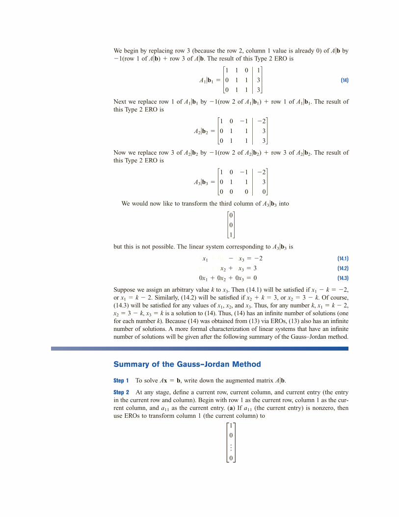
We begin by replacing row 3 (because the row 2, column 1 value is already 0) of A�b by�1(row 1 of A�b) � row 3 of A�b. The result of this Type 2 ERO is

A1�b1 � � � � (14)

Next we replace row 1 of A1�b1 by �1(row 2 of A1�b1) � row 1 of A1�b1. The result ofthis Type 2 ERO is

A2�b2 � � � �Now we replace row 3 of A2�b2 by �1(row 2 of A2�b2) � row 3 of A2�b2. The result ofthis Type 2 ERO is

A3�b3 � � � �We would now like to transform the third column of A3�b3 into

� �but this is not possible. The linear system corresponding to A3�b3 is

0x1 � 0x2 � 0x3 � �2 (14.1)

0x1 � 0x2 � 0x3 � 3 (14.2)

0x1 � 0x2 � 0x3 � 0 (14.3)

Suppose we assign an arbitrary value k to x3. Then (14.1) will be satisfied if x1 � k � �2,or x1 � k � 2. Similarly, (14.2) will be satisfied if x2 � k � 3, or x2 � 3 � k. Of course,(14.3) will be satisfied for any values of x1, x2, and x3. Thus, for any number k, x1 � k � 2,x2 � 3 � k, x3 � k is a solution to (14). Thus, (14) has an infinite number of solutions (onefor each number k). Because (14) was obtained from (13) via EROs, (13) also has an infinitenumber of solutions. A more formal characterization of linear systems that have an infinitenumber of solutions will be given after the following summary of the Gauss–Jordan method.

Summary of the Gauss–Jordan Method

Step 1 To solve Ax � b, write down the augmented matrix A�b.

Step 2 At any stage, define a current row, current column, and current entry (the entryin the current row and column). Begin with row 1 as the current row, column 1 as the cur-rent column, and a11 as the current entry. (a) If a11 (the current entry) is nonzero, thenuse EROs to transform column 1 (the current column) to

� �1

0

��0

0

0

1

�2

3

0

�1

1

0

0

1

0

1

0

0

�2

3

3

�1

1

1

0

1

1

1

0

0

1

3

3

0

1

1

1

1

1

1

0

0


Then obtain the new current row, column, and entry by moving down one row and onecolumn to the right, and go to step 3. (b) If a11 (the current entry) equals 0, then do aType 3 ERO involving the current row and any row that contains a nonzero number in thecurrent column. Use EROs to transform column 1 to

� �Then obtain the new current row, column, and entry by moving down one row and onecolumn to the right. Go to step 3. (c) If there are no nonzero numbers in the first column,then obtain a new current column and entry by moving one column to the right. Then goto step 3.

Step 3 (a) If the new current entry is nonzero, then use EROs to transform it to 1 andthe rest of the current column’s entries to 0. When finished, obtain the new current row,column, and entry. If this is impossible, then stop. Otherwise, repeat step 3. (b) If thecurrent entry is 0, then do a Type 3 ERO with the current row and any row that con-tains a nonzero number in the current column. Then use EROs to transform that cur-rent entry to 1 and the rest of the current column’s entries to 0. When finished, obtainthe new current row, column, and entry. If this is impossible, then stop. Otherwise, re-peat step 3. (c) If the current column has no nonzero numbers below the current row,then obtain the new current column and entry, and repeat step 3. If it is impossible, thenstop.

This procedure may require “passing over” one or more columns without transform-ing them (see Problem 8).

Step 4 Write down the system of equations Ax � b that corresponds to the matrix A�bobtained when step 3 is completed. Then Ax � b will have the same set of solutions asAx � b.

Basic Variables and Solutions to Linear Equation Systems

To describe the set of solutions to Ax � b (and Ax � b), we need to define the conceptsof basic and nonbasic variables.

D E F I N I T I O N ■ After the Gauss–Jordan method has been applied to any linear system, a variablethat appears with a coefficient of 1 in a single equation and a coefficient of 0 inall other equations is called a basic variable (BV). ■

Any variable that is not a basic variable is called a nonbasic variable (NBV). ■

Let BV be the set of basic variables for Ax � b and NBV be the set of nonbasic vari-ables for Ax � b. The character of the solutions to Ax � b depends on which of thefollowing cases occurs.

Case 1 Ax � b has at least one row of form [0 0 �� 0�c] (c 0). Then Ax � b has no solution (recall Example 6). As an example of Case 1, suppose thatwhen the Gauss–Jordan method is applied to the system Ax � b, the following matrixis obtained:

1

0

��0


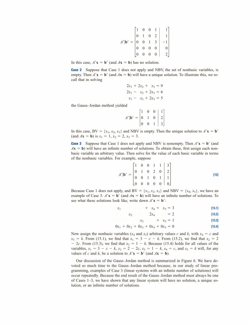
A�b � � � �In this case, Ax � b (and Ax � b) has no solution.

Case 2 Suppose that Case 1 does not apply and NBV, the set of nonbasic variables, isempty. Then Ax � b (and Ax � b) will have a unique solution. To illustrate this, we re-call that in solving

2x1 � 2x2 � x3 � 9

2x1 � x2 � 2x3 � 6

2x1 � x2 � 2x3 � 5

the Gauss–Jordan method yielded

A�b � � � �In this case, BV � {x1, x2, x3} and NBV is empty. Then the unique solution to Ax � b(and Ax � b) is x1 � 1, x2 � 2, x3 � 3.

Case 3 Suppose that Case 1 does not apply and NBV is nonempty. Then Ax � b (andAx � b) will have an infinite number of solutions. To obtain these, first assign each non-basic variable an arbitrary value. Then solve for the value of each basic variable in termsof the nonbasic variables. For example, suppose

A�b � � � � (15)

Because Case 1 does not apply, and BV � {x1, x2, x3} and NBV � {x4, x5}, we have anexample of Case 3: Ax � b (and Ax � b) will have an infinite number of solutions. Tosee what these solutions look like, write down Ax � b:

0x1 � 0x2 � 0x3 � 0x4 � 0x5 � 3 (15.1)

0x1 � 0x2 � 0x3 � 2x4 � 0x5 � 2 (15.2)

0x1 � 0x2 � 0x3 � 0x4 � 0x5 � 1 (15.3)

0x1 � 0x2 � 0x3 � 0x4 � 0x5 � 0 (15.4)

Now assign the nonbasic variables (x4 and x5) arbitrary values c and k, with x4 � c andx5 � k. From (15.1), we find that x1 � 3 � c � k. From (15.2), we find that x2 � 2 � 2c. From (15.3), we find that x3 � 1 � k. Because (15.4) holds for all values of thevariables, x1 � 3 � c � k, x2 � 2 � 2c, x3 � 1 � k, x4 � c, and x5 � k will, for anyvalues of c and k, be a solution to Ax � b (and Ax � b).

Our discussion of the Gauss–Jordan method is summarized in Figure 6. We have de-voted so much time to the Gauss–Jordan method because, in our study of linear pro-gramming, examples of Case 3 (linear systems with an infinite number of solutions) willoccur repeatedly. Because the end result of the Gauss–Jordan method must always be oneof Cases 1–3, we have shown that any linear system will have no solution, a unique so-lution, or an infinite number of solutions.

3

2

1

0

1

0

1

0

1

2

0

0

0

0

1

0

0

1

0

0

1

0

0

0

1

2

3

0

0

1

0

1

0

1

0

0

1

1

�1

0

2

1

2

3

0

0

0

0

1

0

0

0

1

0

0

0

1

0

0

0

0



Use the Gauss–Jordan method to determine whether each ofthe following linear systems has no solution, a unique solu-tion, or an infinite number of solutions. Indicate the solu-tions (if any exist).

1 x1 � x2 � x3 � x4 � 31 x1 � x2 � x3 � x4 � 41 x1 � 2x2 � x3 � x4 � 8

2 x1 � x2 � x3 � 42 x1 � 2x2 � x3 � 6

3 x1 � x2 � 12 2x1 � x2 � 32 3x1 � 2x2 � 4

4 2x1 � x2 � x3 � x4 � 62 x1 � x2 � x3 � x4 � 4

5 x1x2 x2 � x4 � 52 x2x2x 2 � 2x4 � 52 x2x 2x3 � 0.5x4 � 1x2 2x3 � x4 � 3

6 x1 � 2x2 � 2x3 � 42 x1 � 2x2 � x3 � 42 xx1 � 2x2 � x3 � 0

7 x1 � x2 � 2x3 � 22 x1 � x2 � 2x3 � 32 x1 � x2 � x3 � 3

8 x1 � x2 � x3 � x4 � 12 x1 � x2 � 2x3 � x4 � 22 x1 � x2 � 2x3 � x4 � 3

Group B

9 Suppose that a linear system Ax � b has more variablesthan equations. Show that Ax � b cannot have a uniquesolution.

2.4 Linear Independence and Linear Dependence†

In this section, we discuss the concepts of a linearly independent set of vectors, a lin-early dependent set of vectors, and the rank of a matrix. These concepts will be usefulin our study of matrix inverses.

Before defining a linearly independent set of vectors, we need to define a linear com-bination of a set of vectors. Let V � {v1, v2, . . . , vk} be a set of row vectors all ofwhich have the same dimension.

†This section covers topics that may be omitted with no loss of continuity.

YES

YES NO

NO

Does A b have a row [0 0 · · · 0 c] (c ≠ 0)?

Ax = b hasno solution

Find BVand NBV

Is NBVempty?

Ax = b has aunique solution

Ax = b has aninfinite numberof solutions

F I G U R E 6Description of

Gauss–Jordan Methodfor Solving Linear

Equations

P R O B L E M SGroup A

D E F I N I T I O N ■ A linear combination of the vectors in V is any vector of the form c1v1 � c2v2

�� ckvk, where c1, c2, . . . , ck are arbitrary scalars. ■

For example, if V � {[1 2], [2 1]}, then

2v1 � v2 � 2([1 2]) � [2 1] � [0 3]

v1 � 3v2 � [1 2] � 3([2 1]) � [7 5]

0v1 � 3v2 � [0 0] � 3([2 1]) � [6 3]

are linear combinations of vectors in V. The foregoing definition may also be applied toa set of column vectors.

Suppose we are given a set V � {v1, v2, . . . , vk} of m-dimensional row vectors. Let0 � [0 0 �� 0] be the m-dimensional 0 vector. To determine whether V is a linearlyindependent set of vectors, we try to find a linear combination of the vectors in V thatadds up to 0. Clearly, 0v1 � 0v2 � �� 0vk is a linear combination of vectors in V thatadds up to 0. We call the linear combination of vectors in V for which c1 � c2 � �� ck � 0 the trivial linear combination of vectors in V. We may now define linearly inde-pendent and linearly dependent sets of vectors.

D E F I N I T I O N ■ A set V of m-dimensional vectors is linearly independent if the only linearcombination of vectors in V that equals 0 is the trivial linear combination. ■

A set V of m-dimensional vectors is linearly dependent if there is a nontriviallinear combination of the vectors in V that adds up to 0. ■

The following examples should clarify these definitions.

Show that any set of vectors containing the 0 vector is a linearly dependent set.

Solution To illustrate, we show that if V � {[0 0], [1 0], [0 1]}, then V is linearly dependent,because if, say, c1 0, then c1([0 0]) � 0([1 0]) � 0([0 1]) � [0 0]. Thus, thereis a nontrivial linear combination of vectors in V that adds up to 0.

Show that the set of vectors V � {[1 0], [0 1]} is a linearly independent set of vectors.

Solution We try to find a nontrivial linear combination of the vectors in V that yields 0. This re-quires that we find scalars c1 and c2 (at least one of which is nonzero) satisfying c1([1 0]) � c2([0 1]) � [0 0]. Thus, c1 and c2 must satisfy [c1 c2] � [0 0]. Thisimplies c1 � c2 � 0. The only linear combination of vectors in V that yields 0 is the triviallinear combination. Therefore, V is a linearly independent set of vectors.

Show that V � {[1 2], [2 4]} is a linearly dependent set of vectors.

Solution Because 2([1 2]) � 1([2 4]) � [0 0], there is a nontrivial linear combination with c1 � 2 and c2 � �1 that yields 0. Thus, V is a linearly dependent set of vectors.

Intuitively, what does it mean for a set of vectors to be linearly dependent? To understandthe concept of linear dependence, observe that a set of vectors V is linearly dependent (as

2 . 4 Linear Independence and Linear Dependence 33

0 Vector Makes Set LDE X A M P L E 8

LI Set of VectorsE X A M P L E 9

LD Set of VectorsE X A M P L E 1 0

long as 0 is not in V ) if and only if some vector in V can be written as a nontrivial linearcombination of other vectors in V (see Problem 9 at the end of this section). For instance, inExample 10, [2 4] � 2([1 2]). Thus, if a set of vectors V is linearly dependent, the vec-tors in V are, in some way, not all “different” vectors. By “different” we mean that the di-rection specified by any vector in V cannot be expressed by adding together multiples of othervectors in V. For example, in two dimensions it can be shown that two vectors are linearlydependent if and only if they lie on the same line (see Figure 7).

The Rank of a Matrix

The Gauss–Jordan method can be used to determine whether a set of vectors is linearlyindependent or linearly dependent. Before describing how this is done, we define the con-cept of the rank of a matrix.

Let A be any m � n matrix, and denote the rows of A by r1, r2, . . . , rm. Also defineR � {r1, r2, . . . , rm}.

D E F I N I T I O N ■ The rank of A is the number of vectors in the largest linearly independent sub-set of R. ■

The following three examples illustrate the concept of rank.

Show that rank A � 0 for the following matrix:

A � � �Solution For the set of vectors R � {[0 0], [0, 0]}, it is impossible to choose a subset of R that

is linearly independent (recall Example 8).


A � � �1

2

1

2

0

0

0

0


Matrix with Rank of 1E X A M P L E 1 2

Matrix with 0 RankE X A M P L E 1 1

3

2

x2

x1

1

v2v1

A

B

C

v1 = = AB= AC

1 1

1

a

2 3

v2 = 2 23

2

x2

x1

1v2

v1

v2 = 1 1

1

b

2 3

v1 = 1 0

F I G U R E 7(a) Two Linearly

Dependent Vectors (b) Two Linearly

Independent Vectors

Solution Here R � {[1 1], [2 2]}. The set {[1 1]} is a linearly independent subset of R, so rank A must be at least 1. If we try to find two linearly independent vectors in R, we fail because 2([1 1]) � [2 2] � [0 0]. This means that rank A cannot be 2. Thus, rank A must equal 1.


A � � �Solution Here R � {[1 0], [0 1]}. From Example 9, we know that R is a linearly independent

set of vectors. Thus, rank A � 2.

To find the rank of a given matrix A, simply apply the Gauss–Jordan method to thematrix A. Let the final result be the matrix A�. It can be shown that performing a sequenceof EROs on a matrix does not change the rank of the matrix. This implies that rank A �rank AA�. It is also apparent that the rank of A� will be the number of nonzero rows in AA�.Combining these facts, we find that rank A � rank A� � number of nonzero rows in A�.

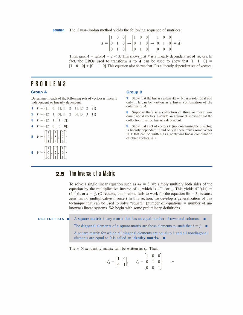
Find

rank A � � �Solution The Gauss–Jordan method yields the following sequence of matrices:

A � � � → � � → � � → � � → � �� A�

Thus, rank A � rank A� � 3.

How to Tell Whether a Set of Vectors Is Linearly Independent

We now describe a method for determining whether a set of vectors V � {v1, v2, . . . , vm}is linearly independent.

Form the matrix A whose ith row is vi. A will have m rows. If rank A � m, then V isa linearly independent set of vectors, whereas if rank A � m, then V is a linearly depen-dent set of vectors.

Determine whether V � {[1 0 0], [0 1 0], [1 1 0]} is a linearly independent setof vectors.

0

0

1

0

1

0

1

0

0

0

�12

�

1

0

1

0

1

0

0

0

�12

�

2

0

1

0

1

0

0

0

�12

�

3

0

1

2

1

0

0

0

1

3

0

2

2

1

0

0

0

1

3

0

2

2

1

0

0

0

1

1

0

2 . 4 Linear Independence and Linear Dependence 35

Using Gauss–Jordan Method to Find Rank of MatrixE X A M P L E 1 4

A Linearly Dependent Set of VectorsE X A M P L E 1 5

Matrix with Rank of 2E X A M P L E 1 3

Solution The Gauss–Jordan method yields the following sequence of matrices:

A � � � → � � → � � � AA�

Thus, rank A � rank AA� � 2 � 3. This shows that V is a linearly dependent set of vectors. Infact, the EROs used to transform A to AA� can be used to show that [1 1 0] �[1 0 0] � [0 1 0]. This equation also shows that V is a linearly dependent set of vectors.


0

0

0

0

1

0

1

0

0

0

0

0

0

1

1

1

0

0

0

0

0

0

1

1

1

0

0


Determine if each of the following sets of vectors is linearlyindependent or linearly dependent.

1 V � {[1 0 1], [1 2 1], [2 2 2]}

2 V � {[2 1 0], [1 2 0], [3 3 1]}

3 V � {[2 1], [1 2]}

4 V � {[2 0], [3 0]}

5 V � �� , � �, � �6 V � �� , � �, � �

101

021

100

579

456

123

Group B

7 Show that the linear system Ax � b has a solution if andonly if b can be written as a linear combination of thecolumns of A.

8 Suppose there is a collection of three or more two-dimensional vectors. Provide an argument showing that thecollection must be linearly dependent.

9 Show that a set of vectors V (not containing the 0 vector)is linearly dependent if and only if there exists some vectorin V that can be written as a nontrivial linear combinationof other vectors in V.

2.5 The Inverse of a MatrixTo solve a single linear equation such as 4x � 3, we simply multiply both sides of theequation by the multiplicative inverse of 4, which is 4�1, or �

14

�. This yields 4�1(4x) �(4�1)3, or x � �

34

�. (Of course, this method fails to work for the equation 0x � 3, becausezero has no multiplicative inverse.) In this section, we develop a generalization of thistechnique that can be used to solve “square” (number of equations � number of un-knowns) linear systems. We begin with some preliminary definitions.

D E F I N I T I O N ■ A square matrix is any matrix that has an equal number of rows and columns. ■

The diagonal elements of a square matrix are those elements aij such that i � j. ■

A square matrix for which all diagonal elements are equal to 1 and all nondiagonalelements are equal to 0 is called an identity matrix. ■

The m � m identity matrix will be written as Im. Thus,

I2 � � �, I3 � � �, ��

0

0

1

0

1

0

1

0

0

0

1

1

0

If the multiplications Im A and AIm are defined, it is easy to show that Im A � AIm � A.Thus, just as the number 1 serves as the unit element for multiplication of real numbers,Im serves as the unit element for multiplication of matrices.

Recall that �14

� is the multiplicative inverse of 4. This is because 4(�14

�) � (�14

�)4 � 1. Thismotivates the following definition of the inverse of a matrix.

D E F I N I T I O N ■ For a given m � m matrix A, the m � m matrix B is the inverse of A if

BA � AB � Im (16)

(It can be shown that if BA � Im or AB � Im, then the other quantity will also equal Im.) ■

Some square matrices do not have inverses. If there does exist an m � m matrix B thatsatisfies Equation (16), then we write B � A�1. For example, if

A � � �the reader can verify that

� �� and

� �� Thus,

A�1 � � �To see why we are interested in the concept of a matrix inverse, suppose we want to

solve a linear system Ax � b that has m equations and m unknowns. Suppose that A�1

exists. Multiplying both sides of Ax � b by A�1, we see that any solution of Ax � b mustalso satisfy A�1(Ax) � A�1b. Using the associative law and the definition of a matrix in-verse, we obtain

(A�1A)x � A�1b

or Imx � A�1b

or Imx � A�1b

This shows that knowing A�1 enables us to find the unique solution to a square linear sys-tem. This is the analog of solving 4x � 3 by multiplying both sides of the equation by 4�1.

The Gauss–Jordan method may be used to find A�1 (or to show that A�1 does not ex-ist). To illustrate how we can use the Gauss–Jordan method to invert a matrix, supposewe want to find A�1 for

A � � �5

3

2

1

1

�7

2

0

1

0

1

�5

1

0

0

1

0

1

0

1

0

0

�1

2

1

0

1

0

2

3

�1

1

�7

2

0

1

0

1

�5

1

0

0

1

0

1

0

1

0

0

1

�7

2

0

1

0

1

�5

1

�1

2

1

0

1

0

2

3

�1

�1

2

1

0

1

0

2

3

�1

2 . 5 The Inverse of a Matrix 37

This requires that we find a matrix

� � � A�1

that satisfies

� �� (17)

From Equation (17), we obtain the following pair of simultaneous equations that mustbe satisfied by a, b, c, and d:

� �� ; � �� Thus, to find

� �(the first column of A�1), we can apply the Gauss–Jordan method to the augmented matrix

� � �Once EROs have transformed

� �to I2,

� �will have been transformed into the first column of A�1. To determine

� �(the second column of A�1), we apply EROs to the augmented matrix

� � �When

� �has been transformed into I2,

� �will have been transformed into the second column of A�1. Thus, to find each column ofA�1, we must perform a sequence of EROs that transform

� �5

3

2

1

0

1

5

3

2

1

0

1

5

3

2

1

b

d

1

0

5

3

2

1

1

0

5

3

2

1

a

c

0

1

b

d

5

3

2

1

1

0

a

c

5

3

2

1

0

1

1

0

b

d

a

c

5

3

2

1

b

d

a

c


into I2. This suggests that we can find A�1 by applying EROs to the 2 � 4 matrix

A�I2 � � � �When

� �has been transformed to I2,

� �will have been transformed into the first column of A�1, and

� �will have been transformed into the second column of A�1. Thus, as A is transformed intoI2, I2 is transformed into A�1. The computations to determine A�1 follow.

Step 1 Multiply row 1 of A�I2 by �12

�. This yields

A�I2� � � �Step 2 Replace row 2 of A�I2 by �1(row 1 of A�I2) � row 2 of A�I2. This yields

A��I�2 � � � �Step 3 Multiply row 2 of A��I�2 by 2. This yields

A �I2 � � � �Step 4 Replace row 1 of A �I2 by ��

52

�(row 2 of A �I2 ) � row 1 of A �I2 . This yields

� � �Because A has been transformed into I2, I2 will have been transformed into A�1. Hence,

A�1 � � �The reader should verify that AA�1 � A�1 A � I2.

A Matrix May Not Have an Inverse

Some matrices do not have inverses. To illustrate, let

A � � � and A�1 � � � (18)f

h

e

g

2

4

1

2

�5

2

3

�1

�5

2

3

�1

0

1

1

0

0

2

�12

�

�1�52

�

11

0

0

1

�12

�

��12

�

�52

�

�12

�

1

0

0

1

�12

�

0

�52

�

3

1

1

0

1

1

0

5

3

2

1

0

1

1

0

5

3

2

1


To find A�1 we must solve the following pair of simultaneous equations:

� �� (18.1)

� �� (18.2)

When we try to solve (18.1) by the Gauss–Jordan method, we find that

� � �is transformed into

� � �This indicates that (18.1) has no solution, and A�1 cannot exist.

Observe that (18.1) fails to have a solution, because the Gauss–Jordan method trans-forms A into a matrix with a row of zeros on the bottom. This can only happen if rank A � 2. If m � m matrix A has rank A � m, then A�1 will not exist.

The Gauss–Jordan Method for Inverting an m � m Matrix A

Step 1 Write down the m � 2m matrix A�Im.

Step 1 Use EROs to transform A�Im into Im�B. This will be possible only if rank A � m.In this case, B � A�1. If rank A � m, then A has no inverse.

Using Matrix Inverses to Solve Linear Systems

As previously stated, matrix inverses can be used to solve a linear system Ax � b in whichthe number of variables and equations are equal. Simply multiply both sides of Ax � bby A�1 to obtain the solution x � A�1b. For example, to solve

2x1 � 5x2 � 7(19)

x1 � 3x2 � 4

write the matrix representation of (19):

� �� (20)

Let

A � � �We found in the previous illustration that

A�1 � � ��5

2

3

�1

5

3

2

1

7

4

x1

x2

5

3

2

1

1

�2

2

0

1

0

1

0

2

4

1

2

0

1

f

h

2

4

1

2

1

0

e

g

2

4

1

2



Multiplying both sides of (20) by A�1, we obtain

� �� 7

4

�5

2

3

�1

x1

x2

5

3

2

1

�5

2

3

�1

123456789

A B C D E F G HInvertingaMatrix 2 0 -1

A 3 1 2-1 0 1

1 0 1A-1 -5 1 -7

1 0 2F I G U R E 8

Find A�1 (if it exists) for the following matrices:

1 � � 2 � �3 � � 4 � �5 Use the answer to Problem 1 to solve the followinglinear system:

x1 � 3x2 � 42x1 � 5x2 � 7

101

224

112

112

011

112

1�2�1

011

143

35

12

6 Use the answer to Problem 2 to solve the followinglinear system:

x1 � x � 2x3 � 44x1 � x2 � 2x3 � 03x1 � x2 � x3 � 2

Group B

7 Show that a square matrix has an inverse if and only ifits rows form a linearly independent set of vectors.

8 Consider a square matrix B whose inverse is given by B�1.a In terms of B�1, what is the inverse of the matrix100B?

� � � � �Thus, x1 � 1, x2 � 1 is the unique solution to system (19).

Inverting Matrices with Excel

The Excel �MINVERSE command makes it easy to invert a matrix. See Figure 8 andfile Minverse.xls. Suppose we want to invert the matrix

A � � �Simply enter the matrix in E3:G5 and select the range (we chose E7:G9) where you want A�1

to be computed. In the upper left-hand corner of the range E7:G9 (cell E7), we enter the formula

� MINVERSE(E3:G5)

and select Control Shift Enter. This enters an array function that computes A�1 in therange E7:G9. You cannot edit part of an array function, so if you want to delete A�1, youmust delete the entire range where A�1 is present.


�1

2

1

0

1

0

2

3

�1

1

1

x1

x2

Minverse.xls

2.6 DeterminantsAssociated with any square matrix A is a number called the determinant of A (often ab-breviated as det A or �A�). Knowing how to compute the determinant of a square matrixwill be useful in our study of nonlinear programming.

For a 1 � 1 matrix A � [a11],

det A � a11 (21)

For a 2 � 2 matrix

A � � � (22)

det A � a11a22 � a21a12

For example,

det � � � 2(5) � 3(4) � �2

Before we learn how to compute det A for larger square matrices, we need to define theconcept of the minor of a matrix.

D E F I N I T I O N ■ If A is an m � m matrix, then for any values of i and j, the ijth minor of A(written Aij) is the (m � 1) � (m � 1) submatrix of A obtained by deleting row iand column j of A. ■

For example,

if A � � �, then A12 � � � and A32 � � �Let A be any m � m matrix. We may write A as

A � � �To compute det A, pick any value of i (i � 1, 2, . . . , m) and compute det A:

det A � (�1)i�1ai1(det Ai1) � (�1)i�2ai2(det Ai2) � �� (�1)i�maim(det Aim) (23)

a1n

a2n

��amn

��

��

��

a12

a22

��am2

a11

a21

��am1

3

6

1

4

6

9

4

7

3

6

9

2

5

8

1

4

7

4

5

2

3

a12

a22

a11

a21


b Let B be the matrix obtained from B by doublingevery entry in row 1 of B. Explain how we could obtainthe inverse of B from B�1.c Let B be the matrix obtained from B by doublingevery entry in column 1 of B. Explain how we could ob-tain the inverse of B from B�1.

9 Suppose that A and B both have inverses. Find the inverseof the matrix AB.

10 Suppose A has an inverse. Show that (AT)�1 � (A�1)T.(Hint: Use the fact that AA�1 � I, and take the transpose ofboth sides.)

11 A square matrix A is orthogonal if AAT � I. Whatproperties must be possessed by the columns of anorthogonal matrix?

2 . 6 Determinants 43

Formula (23) is called the expansion of det A by the cofactors of row i. The virtue of (23) isthat it reduces the computation of det A for an m � m matrix to computations involving only(m � 1) � (m � 1) matrices. Apply (23) until det A can be expressed in terms of 2 � 2 matrices. Then use Equation (22) to find the determinants of the relevant 2 � 2 matrices.

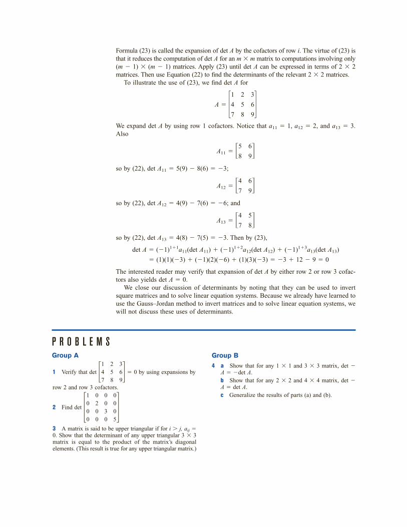
To illustrate the use of (23), we find det A for

A � � �We expand det A by using row 1 cofactors. Notice that a11 � 1, a12 � 2, and a13 � 3.Also

A11 � � �so by (22), det A11 � 5(9) � 8(6) � �3;

A12 � � �so by (22), det A12 � 4(9) � 7(6) � �6; and

A13 � � �so by (22), det A13 � 4(8) � 7(5) � �3. Then by (23),

det A � (�1)1�1a11(det A11) � (�1)1�2a12(det A12) � (�1)1�3a13(det A13)

� (1)(1)(�3) � (�1)(2)(�6) � (1)(3)(�3) � �3 � 12 � 9 � 0

The interested reader may verify that expansion of det A by either row 2 or row 3 cofac-tors also yields det A � 0.

We close our discussion of determinants by noting that they can be used to invertsquare matrices and to solve linear equation systems. Because we already have learned touse the Gauss–Jordan method to invert matrices and to solve linear equation systems, wewill not discuss these uses of determinants.


5

8

4

7

6

9

4

7

6

9

5

8

3

6

9

2

5

8

1

4

7

1 Verify that det � � � 0 by using expansions by

row 2 and row 3 cofactors.

2 Find det � �3 A matrix is said to be upper triangular if for i � j, aij �0. Show that the determinant of any upper triangular 3 � 3matrix is equal to the product of the matrix’s diagonalelements. (This result is true for any upper triangular matrix.)

0005

0030

0200

1000

369

258

147

Group B

4 a Show that for any 1 � 1 and 3 � 3 matrix, det �A � �det A.b Show that for any 2 � 2 and 4 � 4 matrix, det �A � det A.c Generalize the results of parts (a) and (b).

S U M M A R Y Matrices

A matrix is any rectangular array of numbers. For the matrix A, we let aij represent theelement of A in row i and column j.

A matrix with only one row or one column may be thought of as a vector. Vectors ap-pear in boldface type (v). Given a row vector u � [u1 u2 �� un] and a column

v � � �of the same dimension, the scalar product of u and v (written u � v) is the number u1v1 � u2v2 � �� unvn.

Given two matrices A and B, the matrix product of A and B (written AB) is definedif and only if the number of columns in A � the number of rows in B. Suppose this is thecase and A has m rows and B has n columns. Then the matrix product C � AB of A andB is the m � n matrix C whose ijth element is determined as follows: The ijth element ofC � the scalar product of row i of A with column j of B.

Matrices and Linear Equations

The linear equation system

a11x1 � a12x2 � �� a1nxn � b1

a21x1 � a22x2 � �� a2nxn � b2

� � � � �� am1x1 � am2x2 � �� amnxn � bm

may be written as Ax � b or A�b, where

A � � �, x � � �, b � � �The Gauss–Jordan Method

Using elementary row operations (EROs), we may solve any linear equation system.From a matrix A, an ERO yields a new matrix A via one of three procedures.

Type 1 ERO

Obtain A by multiplying any row of A by a nonzero scalar.

Type 2 ERO

Multiply any row of A (say, row i) by a nonzero scalar c. For some j i, let row j of A � c(row i of A) � row j of A, and let the other rows of A be the same as the rows of A.

b1

b2

��bm

x1

x2

��xn

a1n

a2n

��amn

��

��

��

��

a12

a22

��am2

a11

a21

��am1

v1

v2

��vn


Type 3 ERO

Interchange any two rows of A.

The Gauss–Jordan method uses EROs to solve linear equation systems, as shown in thefollowing steps.

Step 1 To solve Ax � b, write down the augmented matrix A�b.

Step 2 Begin with row 1 as the current row, column 1 as the current column, and a11 asthe current entry. (a) If a11 (the current entry) is nonzero, then use EROs to transformcolumn 1 (the current column) to

� �Then obtain the new current row, column, and entry by moving down one row and onecolumn to the right, and go to step 3. (b) If a11 (the current entry) equals 0, then do aType 3 ERO switch with any row with a nonzero value in the same column. Use EROsto transform column 1 to

� �and proceed to step 3 after moving into a new current row, column, and entry. (c) If thereare no nonzero numbers in the first column, then proceed to a new current column andentry. Then go to step 3.

Step 3 (a) If the current entry is nonzero, use EROs to transform it to 1 and the rest ofthe current column’s entries to 0. Obtain the new current row, column, and entry. If thisis impossible, then stop. Otherwise, repeat step 3. (b) If the current entry is 0, then do aType 3 ERO switch with any row with a nonzero value in the same column. Transformthe column using EROs and move to the next current entry. If this is impossible, then stop.Otherwise, repeat step 3. (c) If the current column has no nonzero numbers below the cur-rent row, then obtain the new current column and entry, and repeat step 3. If it is impos-sible, then stop.

This procedure may require “passing over” one or more columns without transform-ing them.

Step 4 Write down the system of equations Ax � b that corresponds to the matrix A�bobtained when step 3 is completed. Then Ax � b will have the same set of solutions asAx � b.

To describe the set of solutions to Ax � b (and Ax � b), we define the concepts ofbasic and nonbasic variables. After the Gauss–Jordan method has been applied to any lin-ear system, a variable that appears with a coefficient of 1 in a single equation and a co-efficient of 0 in all other equations is called a basic variable. Any variable that is not abasic variable is called a nonbasic variable.

1

0

��0

1

0

��0

2 . 5 Summary 45

Let BV be the set of basic variables for Ax � b and NBV be the set of nonbasic vari-ables for Ax � b.

Case 1 Ax � b contains at least one row of the form [0 0 �� 0�c](c 0). In thiscase, Ax � b has no solution.

Case 2 If Case 1 does not apply and NBV, the set of nonbasic variables, is empty, thenAx � b will have a unique solution.

Case 3 If Case 1 does not hold and NBV is nonempty, then Ax � b will have an infi-nite number of solutions.

Linear Independence, Linear Dependence, and the Rank of a Matrix

A set V of m-dimensional vectors is linearly independent if the only linear combinationof vectors in V that equals 0 is the trivial linear combination. A set V of m-dimensionalvectors is linearly dependent if there is a nontrivial linear combination of the vectors inV that adds to 0.

Let A be any m � n matrix, and denote the rows of A by r1, r2, . . . , rm. Also defineR � {r1, r2, . . . , rm}. The rank of A is the number of vectors in the largest linearly in-dependent subset of R. To find the rank of a given matrix A, apply the Gauss–Jordanmethod to the matrix A. Let the final result be the matrix A�. Then rank A � rank A� �number of nonzero rows in A�.

To determine if a set of vectors V � {v1, v2, . . . , vm} is linearly dependent, form thematrix A whose ith row is vi. A will have m rows. If rank A � m, then V is a linearly in-dependent set of vectors; if rank A � m, then V is a linearly dependent set of vectors.

Inverse of a Matrix

For a given square (m � m) matrix A, if AB � BA � Im, then B is the inverse of A (writ-ten B � A�1). The Gauss–Jordan method for inverting an m � m matrix A to get A�1 isas follows:

Step 1 Write down the m � 2m matrix A�Im.

Step 2 Use EROs to transform A�Im into Im�B. This will only be possible if rank A � m.In this case, B � A�1. If rank A � m, then A has no inverse.

Determinants

Associated with any square (m � m) matrix A is a number called the determinant of A(written det A or �A�). For a 1 � 1 matrix, det A � a11. For a 2 � 2 matrix, det A �a11a22 � a21a12. For a general m � m matrix, we can find det A by repeated applicationof the following formula (valid for i � 1, 2, . . . , m):

det A � (�1)i�1ai1(det Ai1) � (�1)i�2ai2(det Ai2) � �� (�1)i�maim(det Aim)

Here Aij is the ijth minor of A, which is the (m � 1) � (m � 1) matrix obtained from Aafter deleting the ith row and jth column of A.


1 Find all solutions to the following linear system:x1 � x2 � x3 � 2x1 � 2x2 � x3 � 3x1 � 2x2 � x3 � 5

2 Find the inverse of the matrix � �.

3 Each year, 20% of all untenured State University facultybecome tenured, 5% quit, and 75% remain untenured. Eachyear, 90% of all tenured S.U. faculty remain tenured and10% quit. Let Ut be the number of untenured S.U. facultyat the beginning of year t, and Tt the tenured number.

Use matrix multiplication to relate the vector � � to

the vector � �.

4 Use the Gauss–Jordan method to determine all solutionsto the following linear system:

2x1 � 3x2 � 3x1 � x2 � 1x1 � 2x2 � 2


6 The grades of two students during their last semester atS.U. are shown in Table 2.

Courses 1 and 2 are four-credit courses, and courses 3and 4 are three-credit courses. Let GPAi be the semestergrade point average for student i. Use matrix multiplication

to express the vector � � in terms of the informationgiven in the problem.

7 Use the Gauss–Jordan method to find all solutions to thefollowing linear system:

2x1 � x2 � 33x1 � x2 � 4x1 � x2 � 0


9 Let Ct � number of children in Indiana at the beginningof year t, and At � number of adults in Indiana at thebeginning of year t. During any given year, 5% of all children

35

23

GPA1

GPA2

23

01

Ut

Tt

Ut�1

Tt�1

31

02

2 . 5 Review Problems 47

become adults, and 1% of all children die. Also, during anygiven year, 3% of all adults die. Use matrix multiplication

to express the vector � � in terms of � �.

10 Use the Gauss–Jordan method to find all solutions tothe following linear equation system:

x1 � x2� x3 � 4x1 �x2 � x3 � 2x1 � x2 � x3� 5

11 Use the Gauss–Jordan method to find the inverse of the

matrix � �.

12 During any given year, 10% of all rural residents moveto the city, and 20% of all city residents move to a rural area(all other people stay put!). Let Rt be the number of ruralresidents at the beginning of year t, and Ct be the numberof city residents at the beginning of year t. Use matrix

multiplication to relate the vector � � to the vector � �.

13 Determine whether the set V � {[1 2 1], [2 0 0]} is a linearly independent set of vectors.

14 Determine whether the set V � {[1 0 0], [0 1 0],[�1 �1 0]} is a linearly independent set of vectors.

15 Let A � � �.a For what values of a, b, c, and d will A�1 exist?b If A�1 exists, then find it.

16 Show that the following linear system has an infinitenumber of solutions:

� �� 17 Before paying employee bonuses and state and federaltaxes, a company earns profits of $60,000. The companypays employees a bonus equal to 5% of after-tax profits.State tax is 5% of profits (after bonuses are paid). Finally,federal tax is 40% of profits (after bonuses and state tax arepaid). Determine a linear equation system to find theamounts paid in bonuses, state tax, and federal tax.

18 Find the determinant of the matrix A � � �.

19 Show that any 2 � 2 matrix A that does not have aninverse will have det A � 0.

601

400

210

2341

x1

x2

x3

x4

0101

0110

1001

1010

000d

00c0

0b00

a000

Rt

Ct

Rt�1

Ct�1

201

011

100

Ct

At

Ct�1

At�1

TA B L E 2

Course

Student 1 2 3 4

1 3.6 3.8 2.6 3.42 2.7 3.1 2.9 3.6

R E V I E W P R O B L E M SGroup A

Group B

20 Let A be an m � m matrix.a Show that if rank A � m, then Ax � 0 has a uniquesolution. What is the unique solution?b Show that if rank A � m, then Ax � 0 has an infi-nite number of solutions.

21 Consider the following linear system:[x1 x2 �� xn] � [x1 x2 �� xn]P

where

P � � �If the sum of each row of the P matrix equals 1, then useProblem 20 to show that this linear system has an infinitenumber of solutions.

22† The national economy of Seriland manufactures threeproducts: steel, cars, and machines. (1) To produce $1 ofsteel requires 30¢ of steel, 15¢ of cars, and 40¢ of machines.(2) To produce $1 of cars requires 45¢ of steel, 20¢ of cars,and 10¢ of machines. (3) To produce $1 of machines requires40¢ of steel, 10¢ of cars, and 45¢ of machines. During thecoming year, Seriland wants to consume ds dollars of steel,dc dollars of cars, and dm dollars of machinery.

For the coming year, lets � dollar value of steel producedc � dollar value of cars producedm � dollar value of machines produced

p1n

p2n

��

pnn

��

��

��

��

p12

p22

��

pn2

p11

p21

��

pn1


Define A to be the 3 � 3 matrix whose ijth element is thedollar value of product i required to produce $1 of productj (steel � product 1, cars � product 2, machinery � prod-uct 3).

a Determine A.b Show that

� � � A� � � � � (24)

(Hint: Observe that the value of next year’s steel production� (next year’s consumer steel demand) � (steel needed tomake next year’s steel) � (steel needed to make next year’scars) � (steel needed to make next year’s machines). Thisshould give you the general idea.)

c Show that Equation (24) may be rewritten as

(I � A)� � � � �d Given values for ds, dc, and dm, describe how youcan use (I � A)�1 to determine if Seriland can meetnext year’s consumer demand.e Suppose next year’s demand for steel increases by$1. This will increase the value of the steel, cars, andmachines that must be produced next year. In terms of(I � A)�1, determine the change in next year’s produc-tion requirements.

ds

dc

dm

sc

m

ds

dc

dm

sc

m

sc

m

R E F E R E N C E SThe following references contain more advanced discus-

sions of linear algebra. To understand the theory of lin-ear and nonlinear programming, master at least one ofthese books:

Dantzig, G. Linear Programming and Extensions. Prince-ton, N.J.: Princeton University Press, 1963.

Hadley, G. Linear Algebra. Reading, Mass.: Addison-Wesley, 1961.

Strang, G. Linear Algebra and Its Applications, 3d ed. Or-lando, Fla.: Academic Press, 1988.

Leontief, W. Input–Output Economics. New York: OxfordUniversity Press, 1966.

Teichroew, D. An Introduction to Management Science: De-terministic Models. New York: Wiley, 1964. A more ex-tensive discussion of linear algebra than this chaptergives (at a comparable level of difficulty).

†Based on Leontief (1966). See references at end of chapter.

basic linear algebra - ufrgs - engenharia de produção ... · basic linear algebra ... the...

Documents