basic econometrics health
TRANSCRIPT
7/30/2019 Basic Econometrics Health
http://slidepdf.com/reader/full/basic-econometrics-health 1/183
*BASIC ECONOMETRICS
*THE NATURE OF LINEAR REGRESSION
Hypothesis testing , and
Estimation

7/30/2019 Basic Econometrics Health
http://slidepdf.com/reader/full/basic-econometrics-health 2/183
2
INTRODUCTION
What is Econometrics?
Econometrics consists of the application of
mathematical statistics to economic data to lend
empirical support to the models constructed bymathematical economics and to obtain numerical
results.
Econometrics may be defined as the quantitativeanalysis of actual economic phenomena based on
the concurrent development of theory and
observation, related by appropriate methods of
inference.

7/30/2019 Basic Econometrics Health
http://slidepdf.com/reader/full/basic-econometrics-health 3/183
3
WHAT IS ECONOMETRICS?
Statistics
Economics
Econometrics
Mathematics

7/30/2019 Basic Econometrics Health
http://slidepdf.com/reader/full/basic-econometrics-health 4/183
4
PURPOSE OF ECONOMETRICS
Structural Analysis
Policy Evaluation
Economic Prediction
Empirical Analysis
7/30/2019 Basic Econometrics Health
http://slidepdf.com/reader/full/basic-econometrics-health 5/183
5
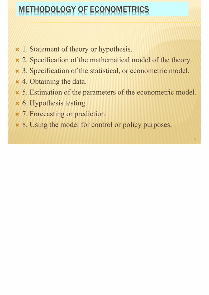
METHODOLOGY OF ECONOMETRICS
1. Statement of theory or hypothesis.
2. Specification of the mathematical model of the theory.
3. Specification of the statistical, or econometric model.
4. Obtaining the data.
5. Estimation of the parameters of the econometric model.
6. Hypothesis testing.
7. Forecasting or prediction.
8. Using the model for control or policy purposes.

7/30/2019 Basic Econometrics Health
http://slidepdf.com/reader/full/basic-econometrics-health 6/183
6
EXAMPLE:KYNESIAN THEORY OF
CONSUMPTION
1. Statement of theory or hypothesis.
Keynes stated: The fundamental psychological law is
that men/women are disposed, as a rule and onaverage, to increase their consumption as their income increases, but not as much as the increasein their income.
In short, Keynes postulated that the marginalpropensity to consume (MPC), the rate of change of consumption for a unit change in income, is greater than zero but less than 1

7/30/2019 Basic Econometrics Health
http://slidepdf.com/reader/full/basic-econometrics-health 7/1837
2.SPECIFICATION OF THE MATHEMATICAL
MODEL OF THE THEORY
A mathematical economist might suggest the
following form of the Keynesian consumption
function:
10 110
X Y
Consumption
expenditure
Income

7/30/2019 Basic Econometrics Health
http://slidepdf.com/reader/full/basic-econometrics-health 8/1838
3. SPECIFICATION OF THE STATISTICAL,
OR ECONOMETRIC MODEL.
To allow for the inexact relationships between
economic variables, the econometrician would modify
the deterministic consumption function as follows:
This is called an econometric model.
u X Y 10
U, known as disturbance, or error term
7/30/2019 Basic Econometrics Health
http://slidepdf.com/reader/full/basic-econometrics-health 9/1839
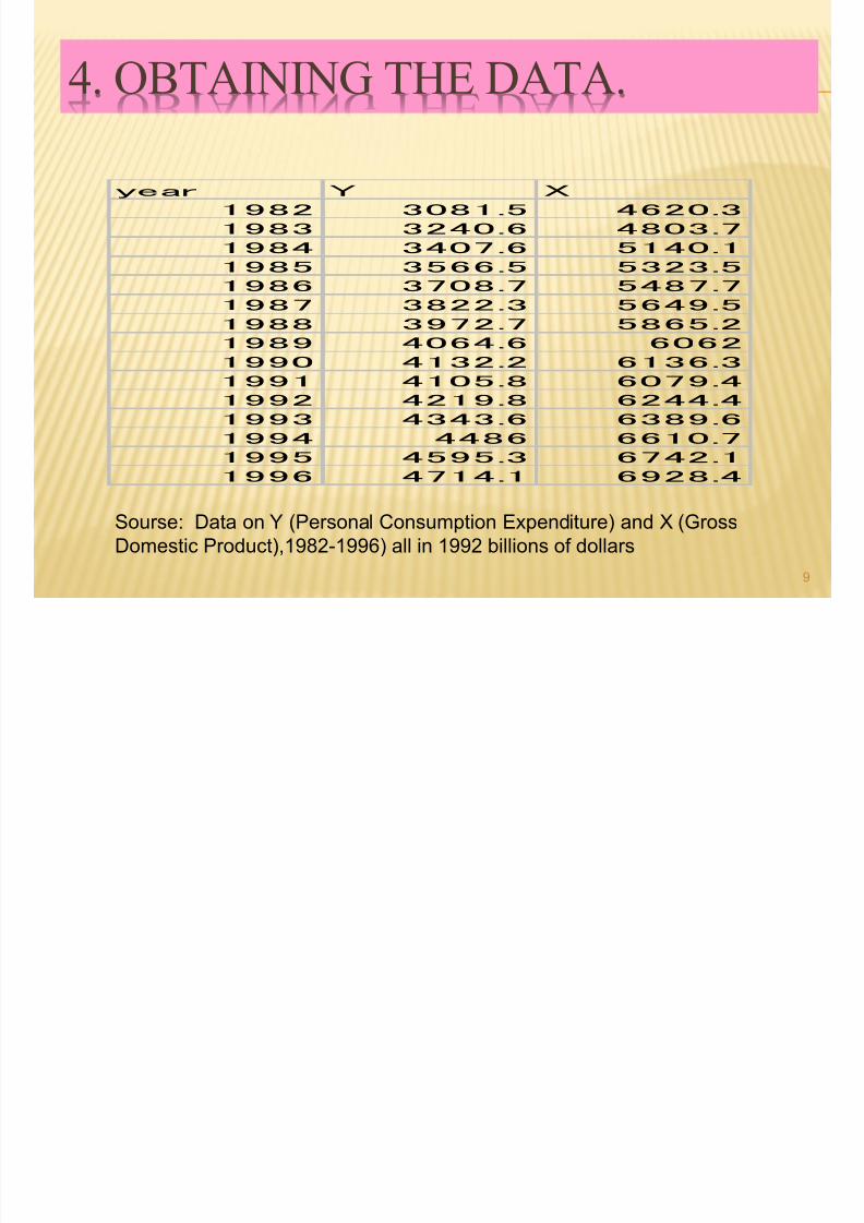
4. OBTAINING THE DATA.
ye ar Y X
1 9 8 2 3 0 8 1 .5 4 6 2 0 .3
1 9 8 3 3 2 4 0 .6 4 8 0 3 .7
1 9 8 4 3 4 0 7 .6 5 1 4 0 .1
1 9 8 5 3 5 6 6 .5 5 3 2 3 .5
1 9 8 6 3 7 0 8 .7 5 4 8 7 .7
1 9 8 7 3 8 2 2 .3 5 6 4 9 .5
1 9 8 8 3 9 7 2 .7 5 8 6 5 .2
1 9 8 9 4 0 6 4 .6 6 0 6 2
1 9 9 0 4 1 3 2 .2 6 1 3 6 .3
1 9 9 1 4 1 0 5 .8 6 0 7 9 .4
1 9 9 2 4 2 1 9 .8 6 2 4 4 .4
1 9 9 3 4 3 4 3 .6 6 3 8 9 .61 9 9 4 4 4 8 6 6 6 1 0 .7
1 9 9 5 4 5 9 5 .3 6 7 4 2 .1
1 9 9 6 4 7 1 4 .1 6 9 2 8 .4
Sourse: Data on Y (Personal Consumption Expenditure) and X (Gross
Domestic Product),1982-1996) all in 1992 billions of dollars

7/30/2019 Basic Econometrics Health
http://slidepdf.com/reader/full/basic-econometrics-health 10/183
10
5. ESTIMATION OF THE PARAMETERS OF
THE ECONOMETRIC MODEL.
reg y x
Source | SS df MS Number of obs = 15
-------------+------------------------------ F( 1, 13) = 8144.59
Model | 3351406.23 1 3351406.23 Prob > F = 0.0000
Residual | 5349.35306 13 411.488697 R-squared = 0.9984 -------------+------------------------------ Adj R-squared = 0.9983
Total | 3356755.58 14 239768.256 Root MSE = 20.285
------------------------------------------------------------------------------
y | Coef. Std. Err. t P>|t| [95% Conf. Interval]
-------------+---------------------------------------------------------------- x | .706408 .0078275 90.25 0.000 .6894978 .7233182
_cons | -184.0779 46.26183 -3.98 0.002 -284.0205 -84.13525
------------------------------------------------------------------------------

7/30/2019 Basic Econometrics Health
http://slidepdf.com/reader/full/basic-econometrics-health 11/183
11
6. HYPOTHESIS TESTING.
Such confirmation or refutation of
econometric theories on the basis of
sample evidence is based on a branch of
statistical theory know as statistical
As noted earlier, Keynes expected the
MPC to be positive but less than 1. In
our example we found it is about 0.70. Then, is 0.70 statistically less than 1?
If it is, it may support keynes’s theory.

7/30/2019 Basic Econometrics Health
http://slidepdf.com/reader/full/basic-econometrics-health 12/183
12
7.FORECASTING OR PREDICTION.
To illustrate, suppose we want to predict the mean
consumption expenditure for 1997. The GDP value
for 1997 was 7269.8 billion dollars. Putting this
value on the right-hand of the model, we obtain4951.3 billion dollars.
But the actual value of the consumption expenditure
reported in 1997 was 4913.5 billion dollars. The
estimated model thus overpredicted.
The forecast error is about 37.82 billion dollars.

7/30/2019 Basic Econometrics Health
http://slidepdf.com/reader/full/basic-econometrics-health 13/183
13
TYPES OF DATA SETS

7/30/2019 Basic Econometrics Health
http://slidepdf.com/reader/full/basic-econometrics-health 14/183
Assume that we have collected data on
two variables X and Y. Let
( x 1
, y 1
) ( x 2
, y 2
) ( x 3
, y 3
) … ( x n
, y n
)
denote the pairs of measurements on the
on two variables X and Y for n cases in a
sample (or population)

7/30/2019 Basic Econometrics Health
http://slidepdf.com/reader/full/basic-econometrics-health 15/183
THE STATISTICAL MODEL

7/30/2019 Basic Econometrics Health
http://slidepdf.com/reader/full/basic-econometrics-health 16/183
Each y i is assumed to be randomlygenerated from a normal distribution with
mean m i = a + x i and
standard deviation s .
(a , and s are unknown)
yi
a + xi
s
xi
Y = a + X
slope =
a

7/30/2019 Basic Econometrics Health
http://slidepdf.com/reader/full/basic-econometrics-health 17/183
THE DATATHE LINEAR REGRESSION MODEL
The data falls roughly about a straight line.
0
20
40
60
80
100
120
140
160
40 60 80 100 120 140
Y = a + X
unseen

7/30/2019 Basic Econometrics Health
http://slidepdf.com/reader/full/basic-econometrics-health 18/183
THE LEAST SQUARES LINE
Fitting the best straight line
to “linear” data
7/30/2019 Basic Econometrics Health
http://slidepdf.com/reader/full/basic-econometrics-health 19/183
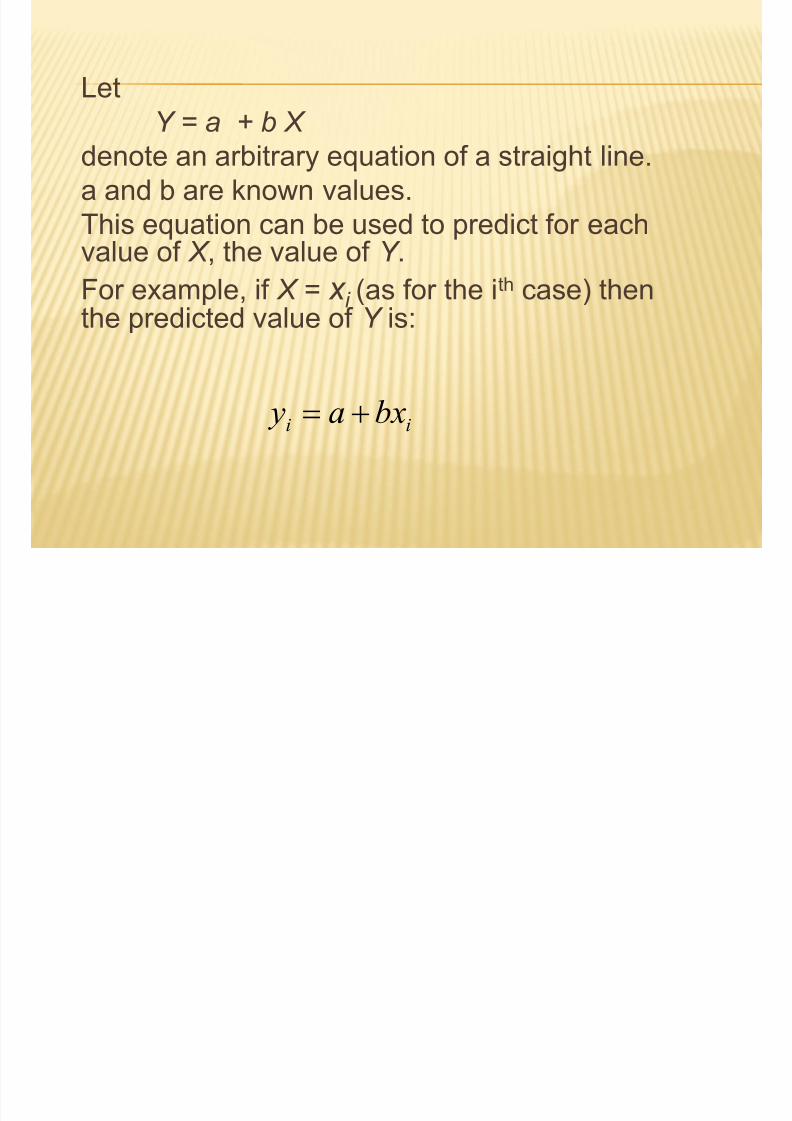
Let
Y = a + b X denote an arbitrary equation of a straight line.
a and b are known values.
This equation can be used to predict for each
value of X , the value of Y .For example, if X = x i (as for the ith case) thenthe predicted value of Y is:
ii bxa y ˆ

7/30/2019 Basic Econometrics Health
http://slidepdf.com/reader/full/basic-econometrics-health 20/183
The residual
can be computed for each case in the sample,
The residual sum of squares (RSS) is
a measure of the “goodness of fit of the lineY = a + bX to the data
iiiii bxa y y yr ˆ
,ˆ,,ˆ,ˆ222111 nnn y yr y yr y yr
n
i
ii
n
i
ii
n
i
i bxa y y yr RSS 1
2
1
2
1
2ˆ

7/30/2019 Basic Econometrics Health
http://slidepdf.com/reader/full/basic-econometrics-health 21/183
7/30/2019 Basic Econometrics Health
http://slidepdf.com/reader/full/basic-econometrics-health 22/183
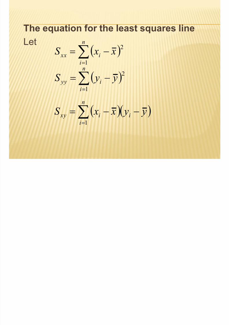
The equation for the least squares line
Let
n
i
i xx x xS 1
2
n
i
i yy y yS 1
2
n
i
ii xy y y x xS 1

7/30/2019 Basic Econometrics Health
http://slidepdf.com/reader/full/basic-econometrics-health 23/183
LINEAR REGRESSION
Hypothesis testing and Estimation
7/30/2019 Basic Econometrics Health
http://slidepdf.com/reader/full/basic-econometrics-health 24/183
THE LEAST SQUARES LINE
Fitting the best straight line
to “linear” data

7/30/2019 Basic Econometrics Health
http://slidepdf.com/reader/full/basic-econometrics-health 25/183
n
x x x xS
n
i
in
i
i
n
i
i xx
2
1
1
2
1
2
n
y x
y x
n
i
i
n
i
in
i
ii
11
1
n
y y y yS
n
i
in
i
i
n
i
i yy
2
1
1
2
1
2
n
i
ii xy y y x xS 1
Computing Formulae:

7/30/2019 Basic Econometrics Health
http://slidepdf.com/reader/full/basic-econometrics-health 26/183
Then the slope of the least squares line
can be shown to be:
n
i
i
n
i
ii
xx
xy
x x
y y x x
S
S b
1
2
1
7/30/2019 Basic Econometrics Health
http://slidepdf.com/reader/full/basic-econometrics-health 27/183
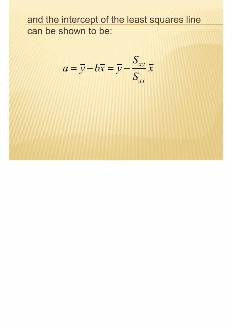
and the intercept of the least squares line
can be shown to be:
x
S
S y xb ya
xx
xy

7/30/2019 Basic Econometrics Health
http://slidepdf.com/reader/full/basic-econometrics-health 28/183
The residual sum of Squares
22
1 1
ˆ
n n
i i i i
i i
RSS y y y a bx
2
xy
yy
xx
S S
S
Computing
formula

7/30/2019 Basic Econometrics Health
http://slidepdf.com/reader/full/basic-econometrics-health 29/183
Estimating s , the standard deviation in the
regression model :
22
ˆ
1
2
1
2
n
bxa y
n
y y
s
n
i
ii
n
i
ii
xx
xy
yy S
S
S n
2
2
1
This estimate of s is said to be based on n – 2
degrees of freedom
Computing
formula

7/30/2019 Basic Econometrics Health
http://slidepdf.com/reader/full/basic-econometrics-health 30/183
SAMPLING DISTRIBUTIONS OF THE
ESTIMATORS

7/30/2019 Basic Econometrics Health
http://slidepdf.com/reader/full/basic-econometrics-health 31/183
The sampling distribution s lope of the
least squares line :
n
i
i
n
i
ii
xx
xy
x x
y y x x
S
S b
1
2
1
It can be shown that b has a normal
distribution with mean and standard deviation
n
i i
xx
bb
x xS
1
2
and s s
s m

7/30/2019 Basic Econometrics Health
http://slidepdf.com/reader/full/basic-econometrics-health 32/183
Thus
has a standard normal distribution, and
b
b
xx
b b z
S
m s s
b
b xx
b bt
s s S
m
has a t distribution with df = n - 2

7/30/2019 Basic Econometrics Health
http://slidepdf.com/reader/full/basic-econometrics-health 33/183
(1 – a )100% Confidence Limits for slope
:
t a /2 critical value for the t-distribution with n – 2
degrees of freedom
xxS
st ˆ
2/a

7/30/2019 Basic Econometrics Health
http://slidepdf.com/reader/full/basic-econometrics-health 34/183
Testing the slope
The test statistic is:
0 0 0: vs : A H H
0
xx
bt
s
S
- has a t distribution with df = n – 2 if H 0 is true.
7/30/2019 Basic Econometrics Health
http://slidepdf.com/reader/full/basic-econometrics-health 35/183
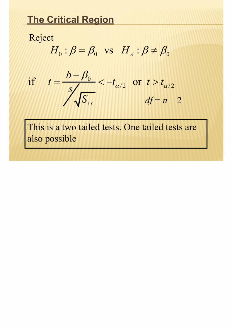
The Critical Region
Reject0 0 0: vs : A H H
0/ 2 / 2if or
xx
bt t t t s
S
a a
df = n – 2
This is a two tailed tests. One tailed tests are
also possible
7/30/2019 Basic Econometrics Health
http://slidepdf.com/reader/full/basic-econometrics-health 36/183
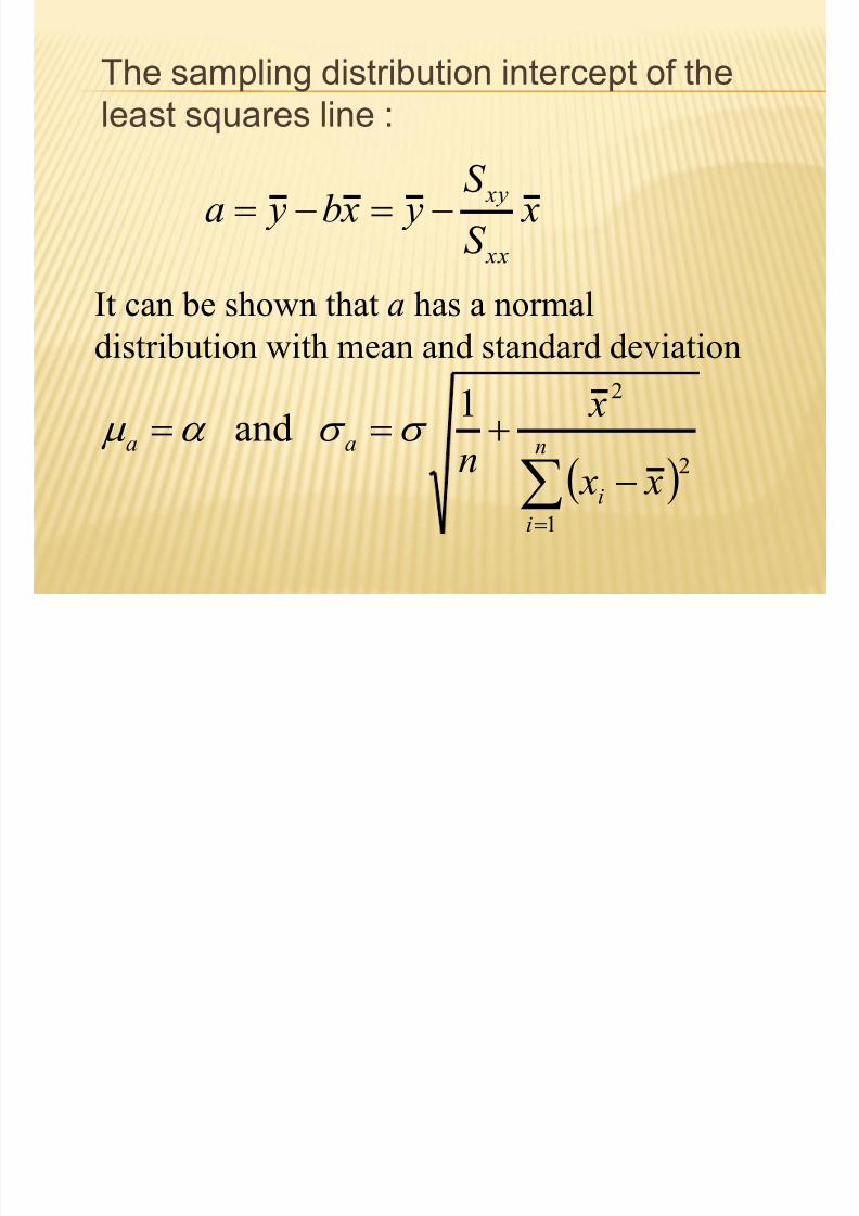
The sampling distribution intercept of the
least squares line :
It can be shown that a has a normal
distribution with mean and standard deviation
n
i
i
aa
x x x
n
1
2
2
1 and s s a m
xS
S y xb ya
xx
xy
7/30/2019 Basic Econometrics Health
http://slidepdf.com/reader/full/basic-econometrics-health 37/183
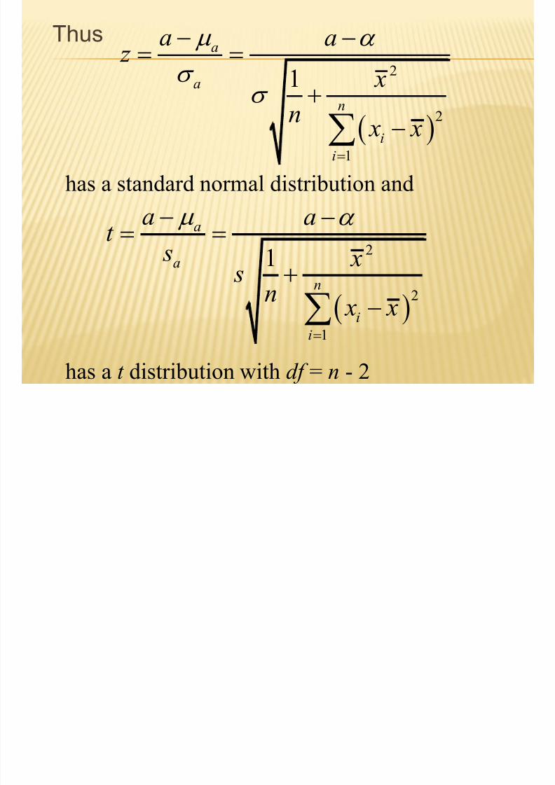
Thus
has a standard normal distribution and
2
2
1
1
a
a
n
i
i
a a z
x
n x x
m a
s
s
2
2
1
1
a
a
n
i
i
a at
s x s n
x x
m a
has a t distribution with df = n - 2

7/30/2019 Basic Econometrics Health
http://slidepdf.com/reader/full/basic-econometrics-health 38/183
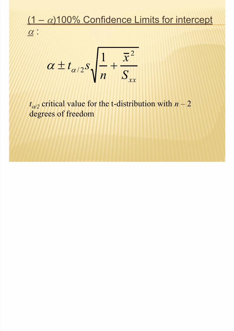
(1 – a )100% Confidence Limits for intercept
a :
t a /2 critical value for the t-distribution with n – 2
degrees of freedom
1ˆ
2
2/
xxS
x
n
st a a

7/30/2019 Basic Econometrics Health
http://slidepdf.com/reader/full/basic-econometrics-health 39/183
Testing the intercept
The test statistic is:
0 0 0: vs : A H H a a a a
- has a t distribution with df = n – 2 if H 0 is true.
0
2
2
1
1
n
i
i
at
x s
n x x
a

7/30/2019 Basic Econometrics Health
http://slidepdf.com/reader/full/basic-econometrics-health 40/183
The Critical Region
Reject0 0 0: vs : A H H a a a a
0/ 2 / 2if or
a
at t t t
sa a
a
df = n – 2

7/30/2019 Basic Econometrics Health
http://slidepdf.com/reader/full/basic-econometrics-health 41/183
EXAMPLE

7/30/2019 Basic Econometrics Health
http://slidepdf.com/reader/full/basic-econometrics-health 42/183
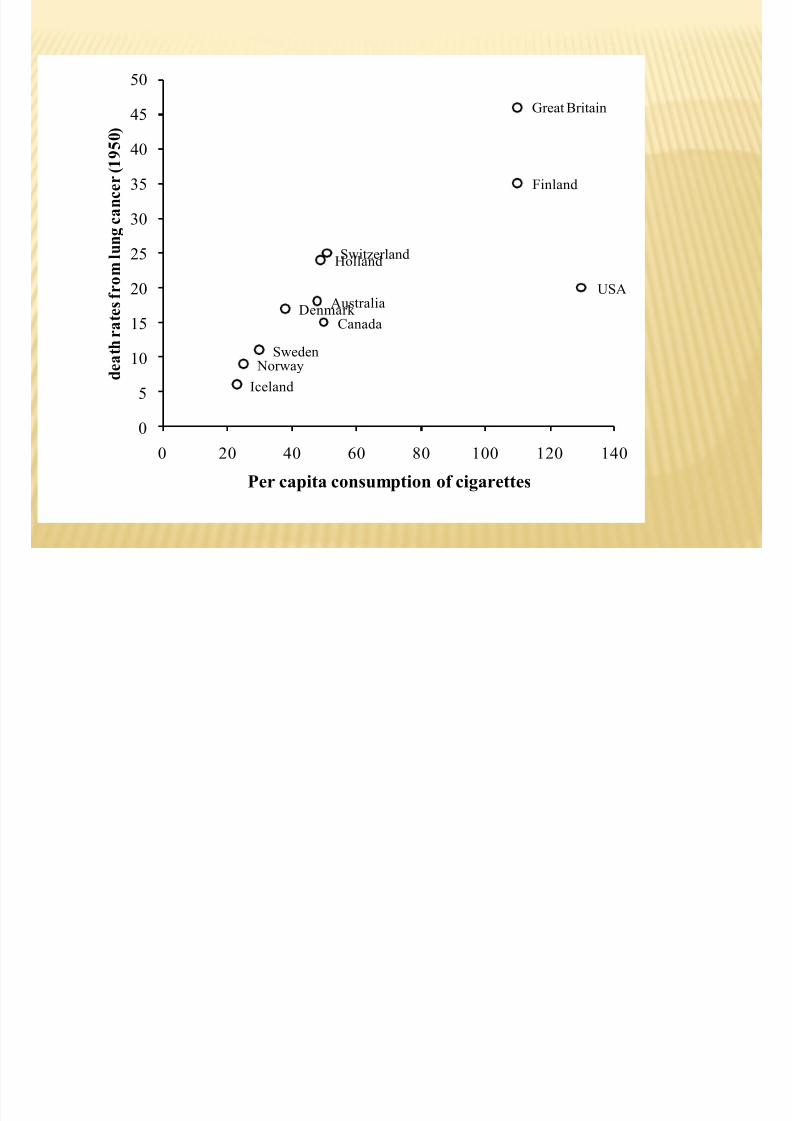
THE FOLLOWING DATA SHOWED THE PER CAPITA CONSUMPTION OF
CIGARETTES PER MONTH (X) IN VARIOUS COUNTRIES IN 1930, AND THE
DEATH RATES FROM LUNG CANCER FOR MEN IN 1950.
TABLE : PER CAPITA CONSUMPTION OF CIGARETTES PER MONTH (XI) IN N
= 11 COUNTRIES IN 1930, AND THE DEATH RATES, Y I (PER 100,000),
FROM LUNG CANCER FOR MEN IN 1950.
COUNTRY (I) XI YI
AUSTRALIA 48 18CANADA 50 15
DENMARK 38 17
FINLAND 110 35
GREAT BRITAIN 110 46
HOLLAND 49 24
ICELAND 23 6
NORWAY 25 9
SWEDEN 30 11
SWITZERLAND 51 25
USA 130 20
7/30/2019 Basic Econometrics Health
http://slidepdf.com/reader/full/basic-econometrics-health 43/183
Australia
CanadaDenmark
Finland
Great Britain
Holland
Iceland
NorwaySweden
Switzerland
USA
0
5
10
15
20
25
30
35
40
45
50
0 20 40 60 80 100 120 140
d e a t h r a t e s f r o m l u
n g c a n c e r ( 1 9 5 0 )
Per capita consumption of cigarettes

7/30/2019 Basic Econometrics Health
http://slidepdf.com/reader/full/basic-econometrics-health 44/183
404,541
2
n
i
i x
914,16
1
n
i
ii y x
018,61
2
n
ii y
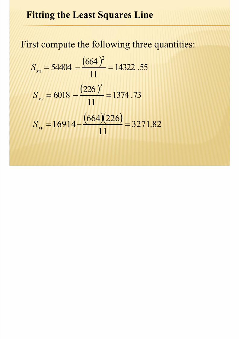
Fitting the Least Squares Line
6641
n
i
i x
2261
n
ii y
7/30/2019 Basic Econometrics Health
http://slidepdf.com/reader/full/basic-econometrics-health 45/183
55.14322
11
66454404
2
xxS
73.1374
11
2266018
2
yyS
82.327111
22666416914 xyS
Fitting the Least Squares Line
First compute the following three quantities:

7/30/2019 Basic Econometrics Health
http://slidepdf.com/reader/full/basic-econometrics-health 46/183
Computing Estimate of Slope (), Intercept (a)
and standard deviation (s),
288.055.14322
82.3271
xx
xy
S
S b
756.611
664288.0
11
226
xb ya
35.82
1 2
xx
xy
yyS
S S
n s

7/30/2019 Basic Econometrics Health
http://slidepdf.com/reader/full/basic-econometrics-health 47/183
95% Confidence Limits for slope :
t .025 = 2.262 critical value for the t-distribution with 9
degrees of freedom
xxS st ˆ
2/a
0.0706 to 0.3862
8.350.288 2.2621432255

7/30/2019 Basic Econometrics Health
http://slidepdf.com/reader/full/basic-econometrics-health 48/183
95% Confidence Limits for intercept a :
1ˆ
2
2/
xxS
x
n st a a
-4.34 to 17.85
t .025 = 2.262 critical value for the t-distribution with 9
degrees of freedom
2664 111
6.756 2.262 8.3511 1432255
50

7/30/2019 Basic Econometrics Health
http://slidepdf.com/reader/full/basic-econometrics-health 49/183
Iceland
NorwaySweden
Denmark Canada
Australia
HollandSwitzerland
Great Britain
Finland
USA
0
5
10
15
20
25
30
35
40
45
50
0 20 40 60 80 100 120 140
Per capita consumption of cigarettes
d e a t h r a t e
s f r o m l u
n g c a n c e
r ( 1 9 5 0
Y = 6.756 + (0.228) X
95% confidence Limits for slope 0.0706 to 0.3862
95% confidence Limits for intercept -4.34 to 17.85
7/30/2019 Basic Econometrics Health
http://slidepdf.com/reader/full/basic-econometrics-health 50/183
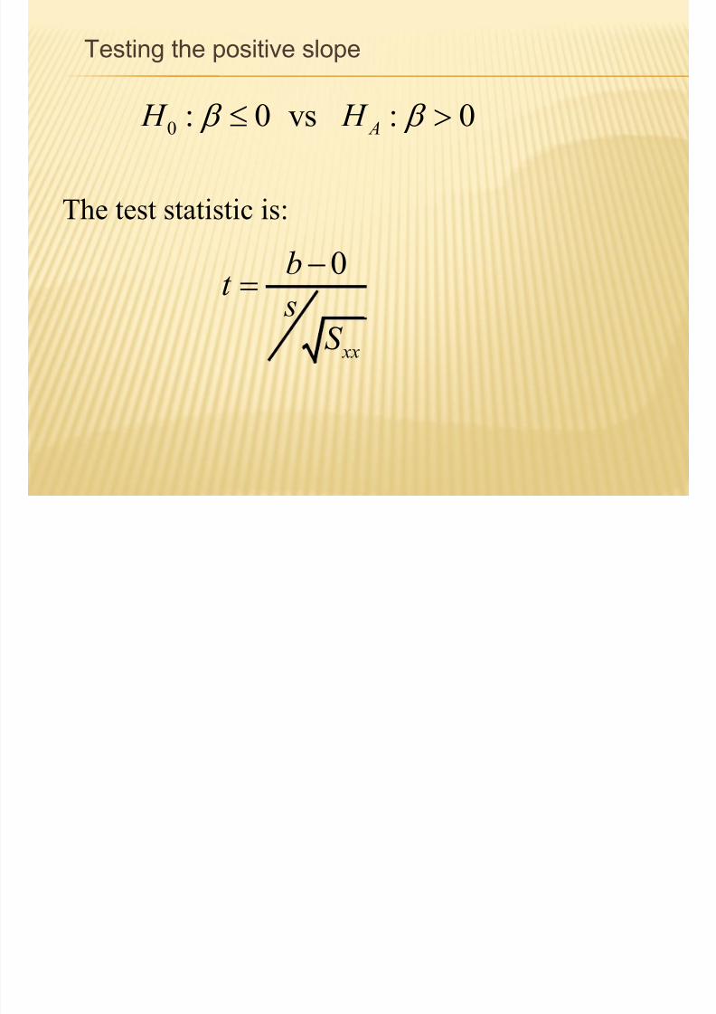
Testing the positive slope
The test statistic is:
0 : 0 vs : 0 A H H
0
xx
bt
s
S

7/30/2019 Basic Econometrics Health
http://slidepdf.com/reader/full/basic-econometrics-health 51/183
The Critical Region
Reject0 : 0 in favour of : 0 A H H
0.050if =1.833
xx
bt t s
S
df = 11 – 2 = 9
A one tailed test
b

7/30/2019 Basic Econometrics Health
http://slidepdf.com/reader/full/basic-econometrics-health 52/183
and conclude
0 : 0 H
0Since
xx
bt
s
S
0.28841.3 1.833
8.35
1432255
we reject
: 0 A H

7/30/2019 Basic Econometrics Health
http://slidepdf.com/reader/full/basic-econometrics-health 53/183
CONFIDENCE LIMITS FOR POINTS ON THE
REGRESSION LINE
The intercept a is a specific point on the regressionline.
It is the y – coordinate of the point on theregression line when x = 0.
It is the predicted value of y when x = 0.
We may also be interested in other points on theregression line. e.g. when x = x 0
In this case the y – coordinate of the point on theregression line when x = x 0 is a + x 0

7/30/2019 Basic Econometrics Health
http://slidepdf.com/reader/full/basic-econometrics-health 54/183
x0
a + x0
y = a + x

7/30/2019 Basic Econometrics Health
http://slidepdf.com/reader/full/basic-econometrics-health 55/183
(1- a )100% Confidence Limits for a + x 0 :
12
02/0
xxS
x x
n
st bxa
a
t a /2 is the a /2 critical value for the t-distribution with
n - 2 degrees of freedom
PREDICTION LIMITS FOR NEW VALUES

7/30/2019 Basic Econometrics Health
http://slidepdf.com/reader/full/basic-econometrics-health 56/183
PREDICTION LIMITS FOR NEW VALUES
OF THE DEPENDENT VARIABLE Y
An important application of the regression line
is prediction.
Knowing the value of x ( x 0) what is the value
of y ? The predicted value of y when x = x 0 is:
This in turn can be estimated by:.
ˆ0 x y a
00 ˆ
ˆˆ bxa x y a

7/30/2019 Basic Econometrics Health
http://slidepdf.com/reader/full/basic-econometrics-health 57/183
The predictor
Gives only a single value for y .
A more appropriate piece of information
would be a range of values.
A range of values that has a fixed
probability of capturing the value for y.
A (1- a )100% predict ion interval for y.
00 ˆˆˆ
bxa x y a

7/30/2019 Basic Econometrics Health
http://slidepdf.com/reader/full/basic-econometrics-health 58/183
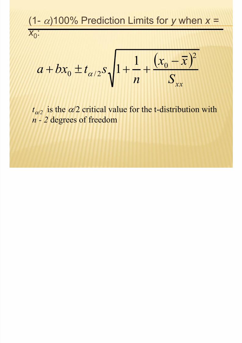
(1- a )100% Prediction Limits for y when x =
x 0:
11
2
02/0
xxS
x x
n
st bxa
a
t a /2 is the a /2 critical value for the t-distribution with
n - 2 degrees of freedom

7/30/2019 Basic Econometrics Health
http://slidepdf.com/reader/full/basic-econometrics-health 59/183
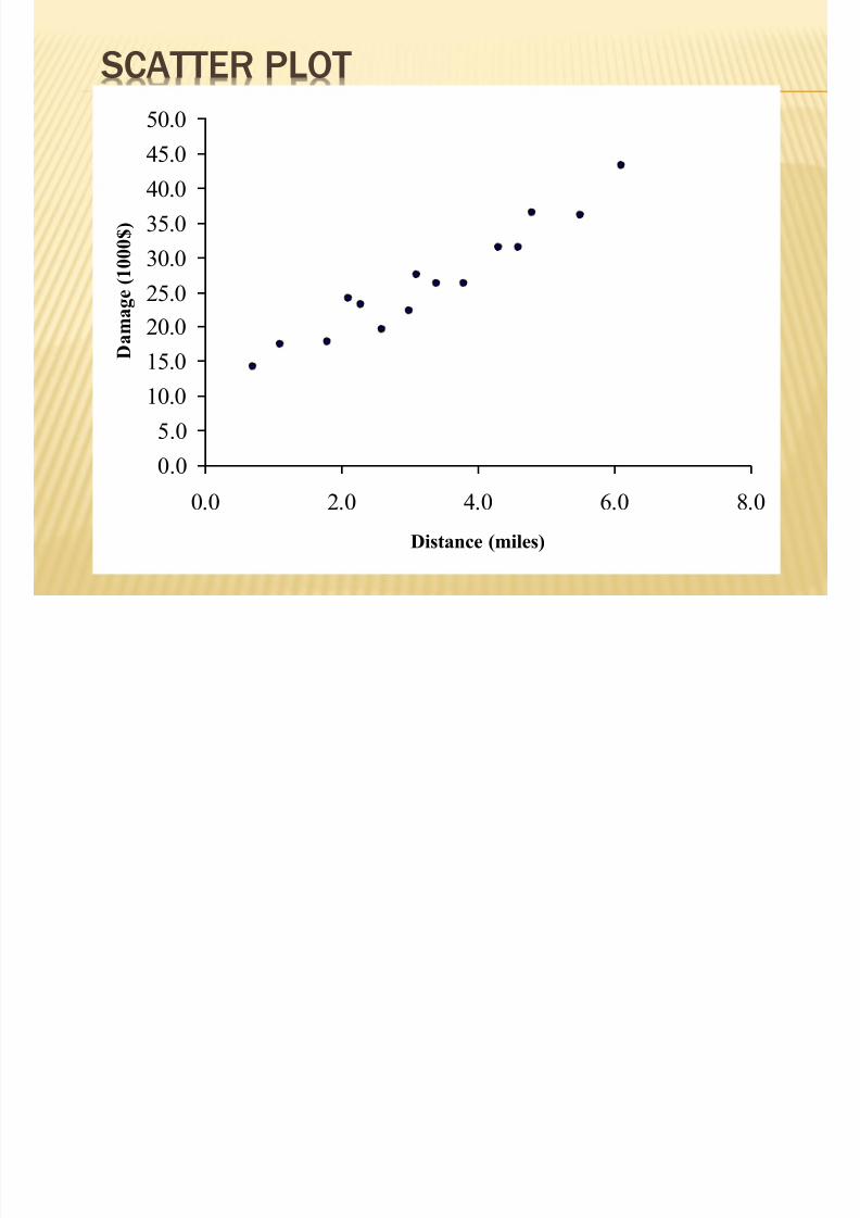
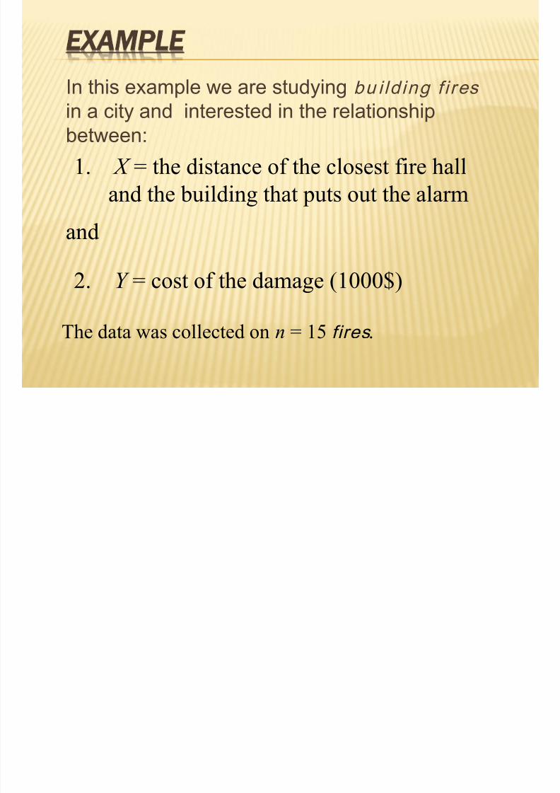
EXAMPLEIn this example we are studying bu i ld ing f i res in a city and interested in the relationship
between:
1. X = the distance of the closest fire hall
and the building that puts out the alarm
and
2. Y = cost of the damage (1000$)
The data was collected on n = 15 fires .

7/30/2019 Basic Econometrics Health
http://slidepdf.com/reader/full/basic-econometrics-health 60/183
THE DATA
Fire Distance Damage1 3.4 26.2
2 1.8 17.8
3 4.6 31.3
4 2.3 23.1
5 3.1 27.5
6 5.5 36.0
7 0.7 14.1
8 3.0 22.3
9 2.6 19.6
10 4.3 31.3
11 2.1 24.012 1.1 17.3
13 6.1 43.2
14 4.8 36.4
15 3.8 26.1
7/30/2019 Basic Econometrics Health
http://slidepdf.com/reader/full/basic-econometrics-health 61/183
SCATTER PLOT
0.0
5.0
10.0
15.0
20.0
25.0
30.0
35.0
40.0
45.0
50.0
0.0 2.0 4.0 6.0 8.0
Distance (miles)
D a m a g e
( 1 0 0 0 $ )

7/30/2019 Basic Econometrics Health
http://slidepdf.com/reader/full/basic-econometrics-health 62/183
COMPUTATIONS
Fire Distance Damage
1 3.4 26.2
2 1.8 17.8
3 4.6 31.3
4 2.3 23.1
5 3.1 27.5
6 5.5 36.0
7 0.7 14.1
8 3.0 22.3
9 2.6 19.6
10 4.3 31.3
11 2.1 24.0
12 1.1 17.3
13 6.1 43.2
14 4.8 36.4
15 3.8 26.1
2.491
n
ii x
2.3961
n
i
i y
65.14701
n
i
ii y x
16.1961
2
n
i
i x
5.113761
2
n
i i
y

7/30/2019 Basic Econometrics Health
http://slidepdf.com/reader/full/basic-econometrics-health 63/183
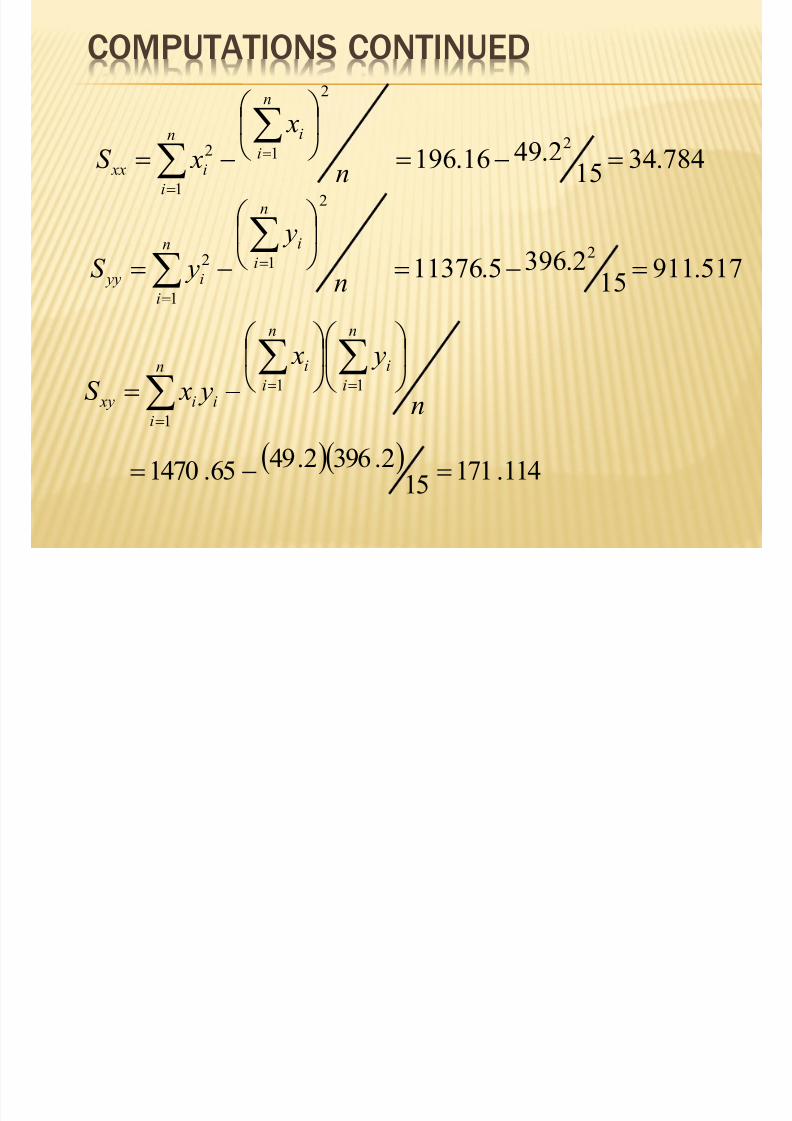
COMPUTATIONS CONTINUED
28.315
2.491
n
x
x
n
i
i
4133.2615
2.3961
n
y
y
n
i
i
COMPUTATIONS CONTINUED
7/30/2019 Basic Econometrics Health
http://slidepdf.com/reader/full/basic-econometrics-health 64/183
COMPUTATIONS CONTINUED
784.3415
2.4916.1962
2
1
1
2
n
x
xS
n
iin
i
i xx
517.911152.3965.113762
2
1
1
2
n
y
yS
n
i
in
i
i yy
n
y x
y xS
n
i
i
n
i
in
i
ii xy
11
1
114.171
152.3962.49
65.1470
COMPUTATIONS CONTINUED

7/30/2019 Basic Econometrics Health
http://slidepdf.com/reader/full/basic-econometrics-health 65/183
COMPUTATIONS CONTINUED
92.4784.34114.171ˆ
xx
xy
S S b
28.1028.3919.44133.26ˆ xb ya a
2
2
n
S
S S
s xx
xy yy
316.213
784.34114.171517.911
2

7/30/2019 Basic Econometrics Health
http://slidepdf.com/reader/full/basic-econometrics-health 66/183
95% Confidence Limits for slope :
t .025 = 2.160 critical value for the t-distribution with
13 degrees of freedom
xxS st ˆ
2/a
4.07 to 5.77

7/30/2019 Basic Econometrics Health
http://slidepdf.com/reader/full/basic-econometrics-health 67/183
95% Confidence Limits for intercept a :
1ˆ
2
2/
xxS
x
n st a a
7.21 to 13.35
t .025 = 2.160 critical value for the t-distribution with
13 degrees of freedom

7/30/2019 Basic Econometrics Health
http://slidepdf.com/reader/full/basic-econometrics-health 68/183
LEAST SQUARES LINE
0.0
10.0
20.0
30.0
40.0
50.0
60.0
0.0 2.0 4.0 6.0 8.0
Distance (miles)
D a m a g e
( 1 0 0 0 $ )
y=4.92 x+10.28

7/30/2019 Basic Econometrics Health
http://slidepdf.com/reader/full/basic-econometrics-health 69/183
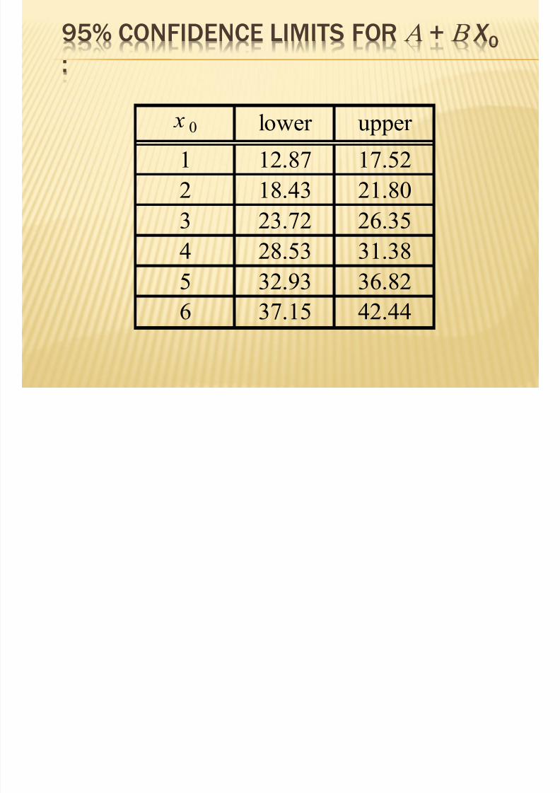
(1- a )100% Confidence Limits for a + x 0 :
12
02/0
xxS
x x
n
st bxa
a
t a /2 is the a /2 critical value for the t-distribution with
n - 2 degrees of freedom
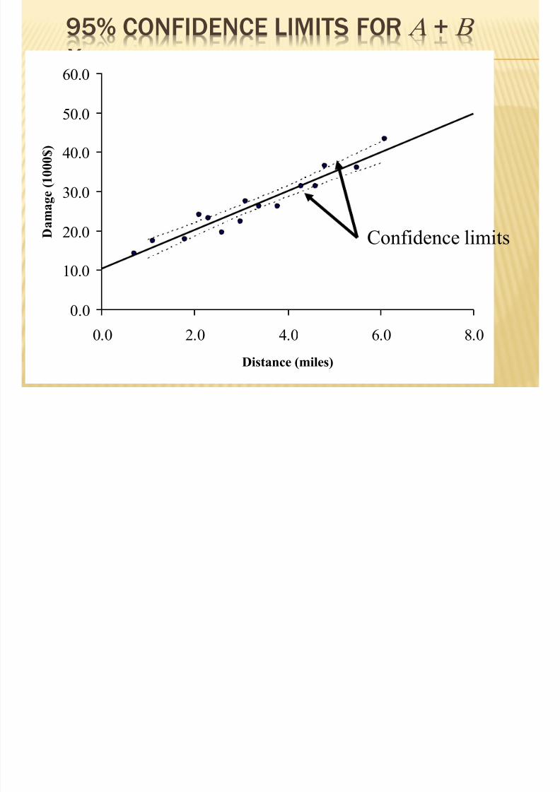
95% CONFIDENCE LIMITS FOR A + B X
7/30/2019 Basic Econometrics Health
http://slidepdf.com/reader/full/basic-econometrics-health 70/183
95% CONFIDENCE LIMITS FOR A + B X 0
:
x 0 lower upper
1 12.87 17.52
2 18.43 21.803 23.72 26.35
4 28.53 31.38
5 32.93 36.826 37.15 42.44
95% CONFIDENCE LIMITS FOR A + B
7/30/2019 Basic Econometrics Health
http://slidepdf.com/reader/full/basic-econometrics-health 71/183
95% CONFIDENCE LIMITS FOR A B
X 0
0.0
10.0
20.0
30.0
40.0
50.0
60.0
0.0 2.0 4.0 6.0 8.0
Distance (miles)
D a m a g e ( 1 0 0 0 $ )
Confidence limits

7/30/2019 Basic Econometrics Health
http://slidepdf.com/reader/full/basic-econometrics-health 72/183
(1- a )100% Prediction Limits for y when x =
x 0:
11
2
02/0
xxS
x x
n
st bxa
a
t a /2 is the a /2 critical value for the t-distribution with
n - 2 degrees of freedom
95% PREDICTION LIMITS FOR Y WHEN X

7/30/2019 Basic Econometrics Health
http://slidepdf.com/reader/full/basic-econometrics-health 73/183
95% PREDICTION LIMITS FOR Y WHEN X =
X 0
x 0 lower upper
1 9.68 20.71
2 14.84 25.403 19.86 30.21
4 24.75 35.16
5 29.51 40.246 34.13 45.45
95% PREDICTION LIMITS FOR Y

7/30/2019 Basic Econometrics Health
http://slidepdf.com/reader/full/basic-econometrics-health 74/183
95% PREDICTION LIMITS FOR Y
WHEN X = X 0
0.0
10.0
20.0
30.0
40.0
50.0
60.0
0.0 2.0 4.0 6.0 8.0
Distance (miles)
D a m a g e ( 1
0 0 0 $ )
Prediction limits
7/30/2019 Basic Econometrics Health
http://slidepdf.com/reader/full/basic-econometrics-health 75/183
LINEAR REGRESSION
SUMMARY
Hypothesis testing and Estimation
7/30/2019 Basic Econometrics Health
http://slidepdf.com/reader/full/basic-econometrics-health 76/183
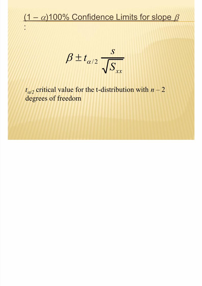
(1 – a )100% Confidence Limits for slope
:
t a /2 critical value for the t-distribution with n – 2
degrees of freedom
xxS
st ˆ
2/a
7/30/2019 Basic Econometrics Health
http://slidepdf.com/reader/full/basic-econometrics-health 77/183
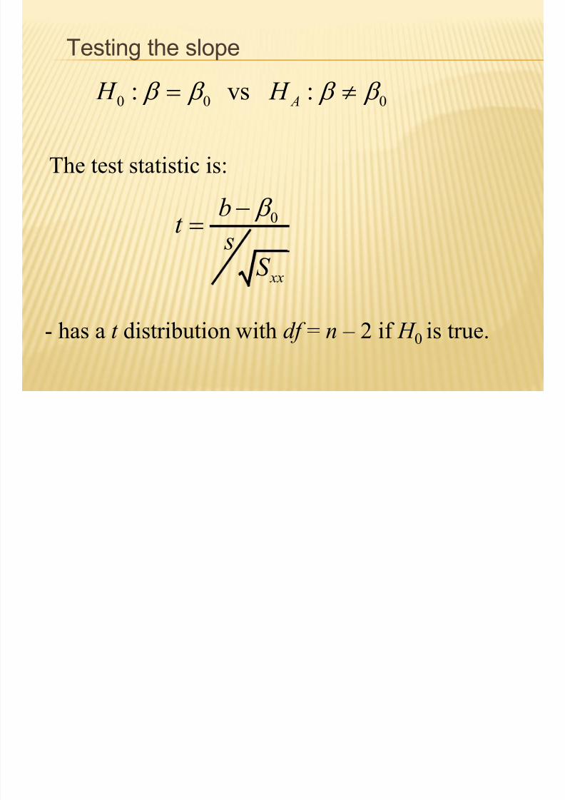
Testing the slope
The test statistic is:
0 0 0: vs : A H H
0
xx
bt
sS
- has a t distribution with df = n – 2 if H 0 is true.
7/30/2019 Basic Econometrics Health
http://slidepdf.com/reader/full/basic-econometrics-health 78/183
(1 – a )100% Confidence Limits for intercept
a :
t a /2 critical value for the t-distribution with n – 2
degrees of freedom
1ˆ
2
2/
xxS
x
n
st a a

7/30/2019 Basic Econometrics Health
http://slidepdf.com/reader/full/basic-econometrics-health 79/183
Testing the intercept
The test statistic is:
0 0 0: vs : A H H a a a a
- has a t distribution with df = n – 2 if H 0is true.
0
2
2
1
1
n
i
i
at x
s
n x x
a

7/30/2019 Basic Econometrics Health
http://slidepdf.com/reader/full/basic-econometrics-health 80/183
(1- a )100% Confidence Limits for a + x 0 :
12
02/0
xxS
x x
n
st bxa
a
t a /2 is the a /2 critical value for the t-distribution with
n - 2 degrees of freedom
7/30/2019 Basic Econometrics Health
http://slidepdf.com/reader/full/basic-econometrics-health 81/183
(1- a )100% Prediction Limits for y when x =
x 0:
11
2
02/0
xxS
x x
n
st bxa
a
t a /2 is the a /2 critical value for the t-distribution with
n - 2 degrees of freedom

7/30/2019 Basic Econometrics Health
http://slidepdf.com/reader/full/basic-econometrics-health 82/183
CORRELATION
Definition
7/30/2019 Basic Econometrics Health
http://slidepdf.com/reader/full/basic-econometrics-health 83/183
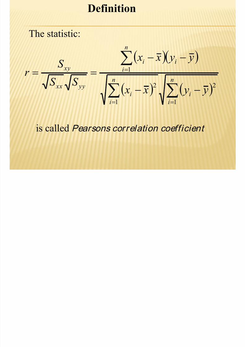
The statistic:
n
i
i
n
i
i
n
i
ii
yy xx
xy
y y x x
y y x x
S S
S r
1
2
1
2
1
is called Pearsons correlation coeff icient

7/30/2019 Basic Econometrics Health
http://slidepdf.com/reader/full/basic-econometrics-health 84/183
The test for independence (zero correlation)

7/30/2019 Basic Econometrics Health
http://slidepdf.com/reader/full/basic-econometrics-health 85/183
The test for independence (zero correlation)
The test statistic:
22
1r t n
r
Reject H 0 if |t | > t a/2 (df = n – 2)
H 0: X and Y are independent
H A: X and Y are correlated
The Critical region
This is a two-tailed critical region, the critical
region could also be one-tailed
7/30/2019 Basic Econometrics Health
http://slidepdf.com/reader/full/basic-econometrics-health 86/183
EXAMPLEIn this example we are studying bu i ld ing f i res
in a city and interested in the relationship
between:
1. X = the distance of the closest fire hall
and the building that puts out the alarm
and
2. Y = cost of the damage (1000$)
The data was collected on n = 15 fires .
THE DATA

7/30/2019 Basic Econometrics Health
http://slidepdf.com/reader/full/basic-econometrics-health 87/183
THE DATA
Fire Distance Damage
1 3.4 26.2
2 1.8 17.8
3 4.6 31.3
4 2.3 23.1
5 3.1 27.5
6 5.5 36.07 0.7 14.1
8 3.0 22.3
9 2.6 19.6
10 4.3 31.3
11 2.1 24.012 1.1 17.3
13 6.1 43.2
14 4.8 36.4
15 3.8 26.1
SCATTER PLOT

7/30/2019 Basic Econometrics Health
http://slidepdf.com/reader/full/basic-econometrics-health 88/183
SCATTER PLOT
0.05.0
10.0
15.0
20.025.0
30.0
35.0
40.045.0
50.0
0.0 2.0 4.0 6.0 8.0
Distance (miles)
D a m a g e
( 1 0 0 0 $ )
COMPUTATIONS

7/30/2019 Basic Econometrics Health
http://slidepdf.com/reader/full/basic-econometrics-health 89/183
COMPUTATIONS
Fire Distance Damage
1 3.4 26.2
2 1.8 17.8
3 4.6 31.3
4 2.3 23.1
5 3.1 27.5
6 5.5 36.0
7 0.7 14.1
8 3.0 22.3
9 2.6 19.6
10 4.3 31.3
11 2.1 24.0
12 1.1 17.3
13 6.1 43.2
14 4.8 36.4
15 3.8 26.1
2.491
n
ii x
2.3961
n
ii y
65.14701
n
i
ii y x
16.1961
2
n
i
i x
5.113761
2
n
i
i y

7/30/2019 Basic Econometrics Health
http://slidepdf.com/reader/full/basic-econometrics-health 90/183
COMPUTATIONS CONTINUED

7/30/2019 Basic Econometrics Health
http://slidepdf.com/reader/full/basic-econometrics-health 91/183
784.3415
2.4916.1962
2
1
1
2
n
x
xS
n
i
in
i
i xx
517.911152.3965.11376
2
2
1
1
2
n
y
yS
n
i
in
i
i yy
n
y x
y xS
n
i
i
n
i
in
iii xy
11
1
114.171
152.3962.49
65.1470
THE CORRELATION COEFFICIENT

7/30/2019 Basic Econometrics Health
http://slidepdf.com/reader/full/basic-econometrics-health 92/183
171.114
0.96134.784 911.517
xy
xx yy
S
r S S
The test for independence (zero correlation)
The test statistic:
2 2
0.9612 13 12.525
1 1 0.961
r t n
r
We reject H 0: independence, if |t | > t 0.025 = 2.160
H 0: independence, is rejected
7/30/2019 Basic Econometrics Health
http://slidepdf.com/reader/full/basic-econometrics-health 93/183
RELATIONSHIP BETWEEN REGRESSION
AND CORRELATION
Recall xyS r

7/30/2019 Basic Econometrics Health
http://slidepdf.com/reader/full/basic-econometrics-health 94/183
Recall
xx yy
r S S
Also
ˆxy yy xy yy y
xx xx xx x xx yy
S S S S sr r
S S S sS S
since and
1 1
yy xx x y
S S s s
n n
Thus the slope of the least squares line is simply the ratio
of the standard deviations × the correlation coefficient
The test for independence (zero correlation)

7/30/2019 Basic Econometrics Health
http://slidepdf.com/reader/full/basic-econometrics-health 95/183
The test for independence (zero correlation)
Uses the test statistic:
22
1r t n
r
H 0: X and Y are independent
H A: X and Y are correlated
Note: andˆ yy
xx
S r S
ˆ xx
yy
S r S
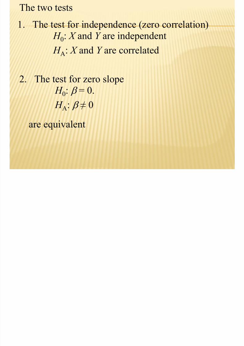
The two tests
7/30/2019 Basic Econometrics Health
http://slidepdf.com/reader/full/basic-econometrics-health 96/183
1. The test for independence (zero correlation) H 0: X and Y are independent
H A: X and Y are correlated
are equivalent
2. The test for zero slope H 0: = 0.
H A: ≠ 0
1. the test statistic for independence:

7/30/2019 Basic Econometrics Health
http://slidepdf.com/reader/full/basic-econometrics-health 97/183
22
1
r t n
r
2 22 2
1 1
xy xy
xx yy xx
xy xy yy
xx yy xx yy
S S
S S S t n n
S S S S S S S
Thus
2
ˆ
12
the same statistic for testing for slope.
xy
xx
xy
yy xx
xx xx
S
S
sS S n S
S S
zero

7/30/2019 Basic Econometrics Health
http://slidepdf.com/reader/full/basic-econometrics-health 98/183
REGRESSION (IN GENERAL)
In many experiments we would have collected data on a
7/30/2019 Basic Econometrics Health
http://slidepdf.com/reader/full/basic-econometrics-health 99/183
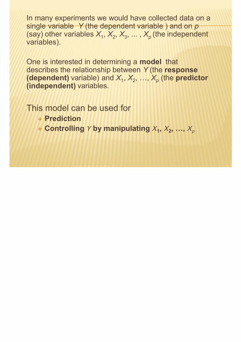
In many experiments we would have collected data on asingle variable Y (the dependent variable ) and on p (say) other variables X 1, X 2, X 3, ... , X p (the independent
variables).
One is interested in determining a model thatdescribes the relationship between Y (the response(dependent) variable) and X
1
, X 2
, …, X p
(the predictor (independent) variables.
This model can be used for
Prediction Controlling Y by manipulating X 1, X 2, …, X p

7/30/2019 Basic Econometrics Health
http://slidepdf.com/reader/full/basic-econometrics-health 100/183
The Model:
is an equation of the form
Y = f ( X 1, X 2,... , X p | q1, q2, ... , qq) + e
where q1, q2, ... , qq are unknownparameters of the function f and e is arandom disturbance (usually assumed to
have a normal distribution with mean 0and standard deviation s.

7/30/2019 Basic Econometrics Health
http://slidepdf.com/reader/full/basic-econometrics-health 101/183
2. Y = average of five best times for running
the 100m X the ear

7/30/2019 Basic Econometrics Health
http://slidepdf.com/reader/full/basic-econometrics-health 102/183
8
8.5
9
9.5
10
10.5
11
11.5
12
12.5
1930 1940 1950 1960 1970 1980 1990 2000 2010
the 100m, X = the year
The model
Y = a e- X + g e, thus q1 = a, q2 = and q2 =
g .
This model is called:
the exponential Regression Model
Y = a e- X + g

7/30/2019 Basic Econometrics Health
http://slidepdf.com/reader/full/basic-econometrics-health 103/183
7/30/2019 Basic Econometrics Health
http://slidepdf.com/reader/full/basic-econometrics-health 104/183
THE MULTIPLE LINEAR
REGRESSION MODEL
In Multiple Linear Regression we assume the

7/30/2019 Basic Econometrics Health
http://slidepdf.com/reader/full/basic-econometrics-health 105/183
In Multiple Linear Regression we assume thefollowing model
Y = 0 + 1 X1 + 2 X2 + ... + p Xp + e
This model is called the Multiple Linear Regression Model.
Again are unknown parameters of the modeland where 0, 1, 2, ... , p are unknownparameters and e is a random disturbanceassumed to have a normal distribution withmean 0 and standard deviation s.
THE IMPORTANCE OF THE LINEAR MODEL
7/30/2019 Basic Econometrics Health
http://slidepdf.com/reader/full/basic-econometrics-health 106/183
THE IMPORTANCE OF THE LINEAR MODEL
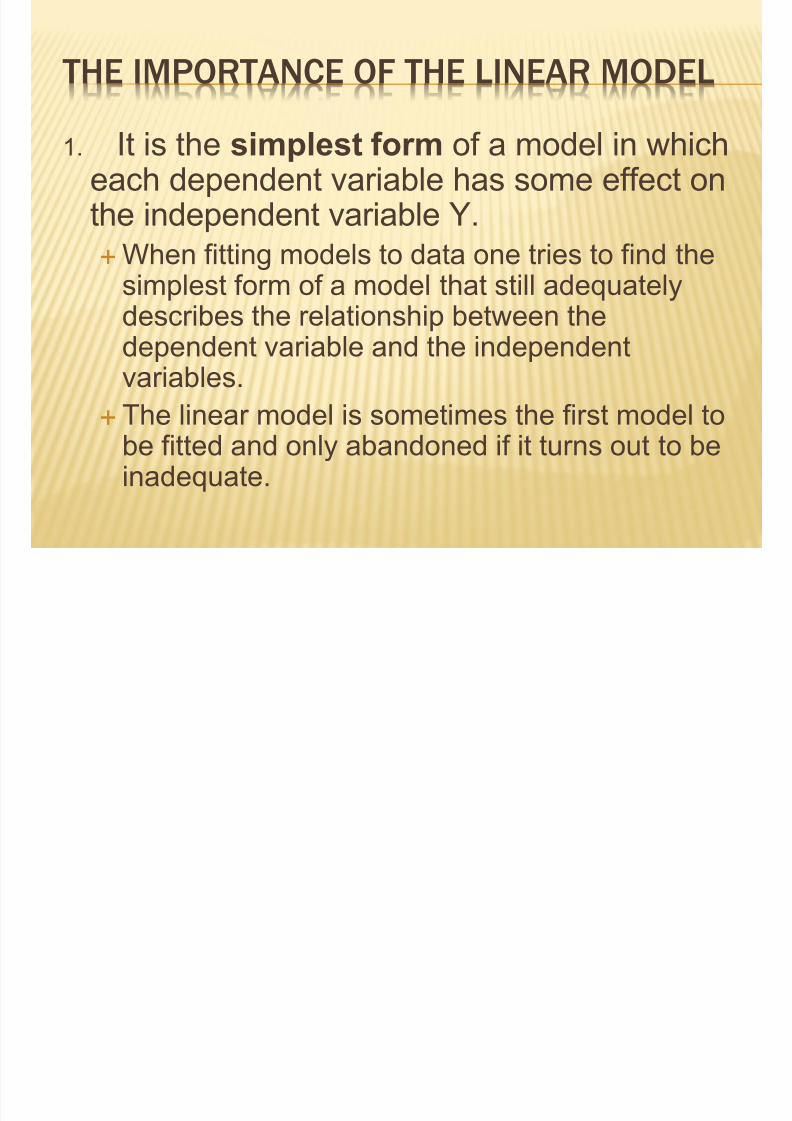
1. It is the simplest form of a model in whicheach dependent variable has some effect onthe independent variable Y.
When fitting models to data one tries to find thesimplest form of a model that still adequatelydescribes the relationship between thedependent variable and the independentvariables.
The linear model is sometimes the first model tobe fitted and only abandoned if it turns out to beinadequate.
I i t li d l i th

7/30/2019 Basic Econometrics Health
http://slidepdf.com/reader/full/basic-econometrics-health 107/183
2. In many instance a linear model is the
most appropriate model to describe
the dependence relationship betweenthe dependent variable and the
independent variables.
This will be true if the dependent variableincreases at a constant rate as any or the
independent variables is increased while
holding the other independent variables
constant.
3 Man non Linear models can be

7/30/2019 Basic Econometrics Health
http://slidepdf.com/reader/full/basic-econometrics-health 108/183
3. Many non-Linear models can be
Linearized (put into the form of a
Linear model by appropriatelytransformation the dependent variables
and/or any or all of the independent
variables.) This important fact ensures the wide utility
of the Linear model. (i.e. the fact the many
non-linear models are linearizable.)

7/30/2019 Basic Econometrics Health
http://slidepdf.com/reader/full/basic-econometrics-health 109/183
AN EXAMPLE
The following data comes from an experimentthat was interested in investigating the sourcefrom which corn plants in various soils obtaintheir phosphorous.
The concentration of inorganic phosphorous (X1)and the concentration of organic phosphorous (X2)was measured in the soil of n = 18 test plots.
In addition the phosphorous content (Y) of corngrown in the soil was also measured. The data isdisplayed below:

7/30/2019 Basic Econometrics Health
http://slidepdf.com/reader/full/basic-econometrics-health 110/183
Inorganic
Phosphorous
X1
Organic
Phosphorous
X2
Plant
Available
Phosphorous Y
Inorganic
Phosphorous
X1
Organic
Phosphorous
X2
Plant
Available
Phosphorous Y
0.4 53 64 12.6 58 51
0.4 23 60 10.9 37 76
3.1 19 71 23.1 46 96 0.6 34 61 23.1 50 77
4.7 24 54 21.6 44 93
1.7 65 77 23.1 56 95
9.4 44 81 1.9 36 54
10.1 31 93 26.8 58 168
11.6 29 93 29.9 51 99
7/30/2019 Basic Econometrics Health
http://slidepdf.com/reader/full/basic-econometrics-health 111/183
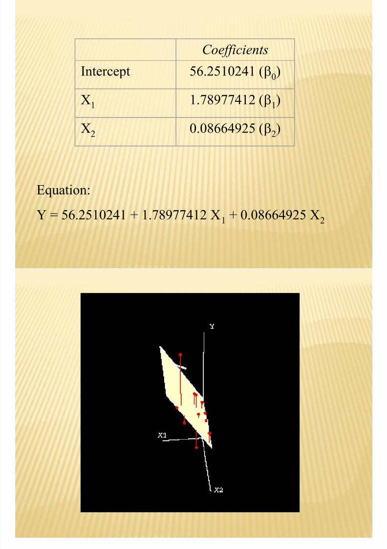
Coefficients
Intercept 56.2510241 (0)
X1 1.78977412 (1)
X2 0.08664925 (2)
Equation:Y = 56.2510241 + 1.78977412 X1 + 0.08664925 X2

7/30/2019 Basic Econometrics Health
http://slidepdf.com/reader/full/basic-econometrics-health 112/183

7/30/2019 Basic Econometrics Health
http://slidepdf.com/reader/full/basic-econometrics-health 113/183
THE MULTIPLE LINEAR
REGRESSION MODEL
In Multiple Linear Regression we assume the
7/30/2019 Basic Econometrics Health
http://slidepdf.com/reader/full/basic-econometrics-health 114/183
In Multiple Linear Regression we assume thefollowing model
Y = 0 + 1 X1 + 2 X2 + ... + p Xp + e
This model is called the Multiple Linear Regression Model.
Again are unknown parameters of the modeland where 0, 1, 2, ... , p are unknownparameters and e is a random disturbanceassumed to have a normal distribution withmean 0 and standard deviation s.
SUMMARY OF THE STATISTICS

7/30/2019 Basic Econometrics Health
http://slidepdf.com/reader/full/basic-econometrics-health 115/183
USED IN
MULTIPLE REGRESSION
The Least Squares Estimates:
7/30/2019 Basic Econometrics Health
http://slidepdf.com/reader/full/basic-econometrics-health 116/183
q
0 1 2, , , , , p
2
1
ˆ
n
i i
i
RSS y y
2
0 1 1 2 2
1
n
i i i p pi
i
y x x x
- the values that minimize
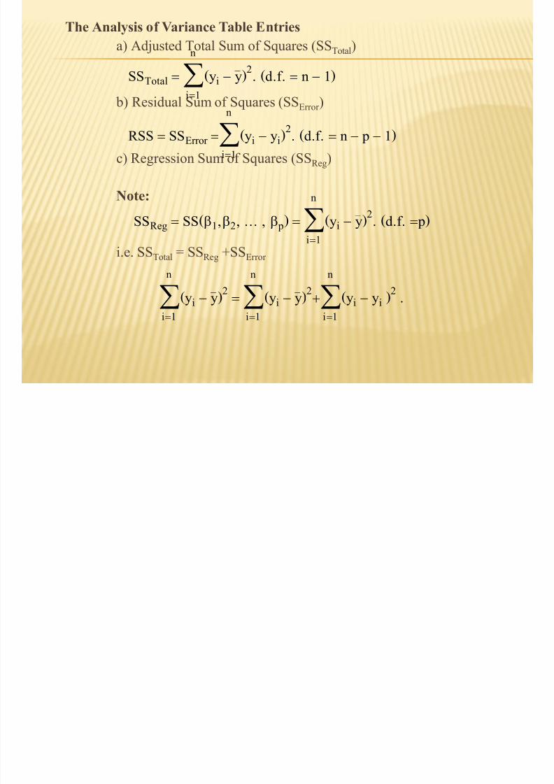
The Analysis of Variance Table Entries
a) Adjusted Total Sum of Squares (SSTotal)n

7/30/2019 Basic Econometrics Health
http://slidepdf.com/reader/full/basic-econometrics-health 117/183
b) Residual Sum of Squares (SSError )
c) Regression Sum of Squares (SSReg)
Note:
i.e. SSTotal = SSReg +SSError
SSTotal n
i1
yi y _
2. d.f. n 1
RSS SSError n
i1
yi yˆi2. d.f. n p 1
SSReg SS1,2, ... , p n
i1
yˆ i y _
2. d.f. p
n
i1
yi y _
2
n
i1
yˆi y _
2
n
i1
yi yˆi 2
.
THE ANALYSIS OF VARIANCE TABLE

7/30/2019 Basic Econometrics Health
http://slidepdf.com/reader/full/basic-econometrics-health 118/183
Source Sum of Squares d.f. Mean Square F
Regression SSReg p SSReg /p = MSReg MSReg /s2
Error SSError n-p-1 SSError /(n-p-1) =MSError = s2
Total SSTotal n-1
USES:
7/30/2019 Basic Econometrics Health
http://slidepdf.com/reader/full/basic-econometrics-health 119/183
1. To estimate s2 (the error variance).
- Use s2 = MSError to estimate s2.
2. To test the Hypothesis
H0: 1 = 2= ... = p = 0.
Use the test statistic
2
Reg Reg Error F MS MS MS s
Reg 1 Error SS p SS n p
- Reject H 0 if F > F a ( p,n-p-1).
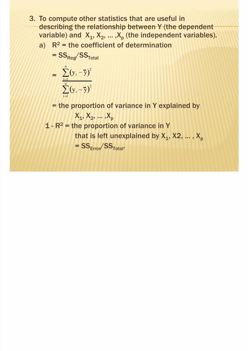
3. To compute other statistics that are useful indescribing the relationship between Y (the dependent

7/30/2019 Basic Econometrics Health
http://slidepdf.com/reader/full/basic-econometrics-health 120/183
describing the relationship between Y (the dependent
variable) and X1, X2, ... ,Xp (the independent variables).
a) R2
= the coefficient of determination= SSReg /SSTotal
=
= the proportion of variance in Y explained by
X1, X2, ... ,Xp
1 - R2 = the proportion of variance in Y that is left unexplained by X1, X2, ... , Xp
= SSError /SSTotal.
y i y 2i1
n
y i y 2
i1
n

7/30/2019 Basic Econometrics Health
http://slidepdf.com/reader/full/basic-econometrics-health 121/183
b) Ra2 = "R2 adjusted" for degrees of freedom.
= 1 -[the proportion of variance in Y that is leftunexplained by X1, X2,... , Xp adjusted for d.f.]
1 Error Total MS MS
11
1
Error
Total
SS n p
SS n
11
1
Error
Total
n SS
n p SS
2
11 1
1
n R
n p
c) R= R2 = the Multiple correlation coefficient of

7/30/2019 Basic Econometrics Health
http://slidepdf.com/reader/full/basic-econometrics-health 122/183
Y with X 1, X 2, ... , X p
=
= the maximum correlation between Y and a
linear combination of X 1, X 2, ... , X p
Comment: The statistics F, R 2, R a2 and R are
equivalent statistics.
SSRe g
SSTotal

7/30/2019 Basic Econometrics Health
http://slidepdf.com/reader/full/basic-econometrics-health 123/183
USING STATISTICAL PACKAGES
To perform Multiple Regression

7/30/2019 Basic Econometrics Health
http://slidepdf.com/reader/full/basic-econometrics-health 124/183
USING SPSS
Note: The use of another statistical package
such as Minitab is similar to using SPSS
AFTER STARTING THE SSPS PROGRAM THE FOLLOWING
DIALOGUE BOX APPEARS:

7/30/2019 Basic Econometrics Health
http://slidepdf.com/reader/full/basic-econometrics-health 125/183
DIALOGUE BOX APPEARS:
IF YOU SELECT OPENING AN EXISTING FILE AND PRESS OK
THE FOLLOWING DIALOGUE BOX APPEARS

7/30/2019 Basic Econometrics Health
http://slidepdf.com/reader/full/basic-econometrics-health 126/183
THE FOLLOWING DIALOGUE BOX APPEARS:

7/30/2019 Basic Econometrics Health
http://slidepdf.com/reader/full/basic-econometrics-health 127/183
IF THE VARIABLE NAMES ARE IN THE FILE ASK IT TO
READ THE NAMES IF YOU DO NOT SPECIFY THE

7/30/2019 Basic Econometrics Health
http://slidepdf.com/reader/full/basic-econometrics-health 128/183
READ THE NAMES. IF YOU DO NOT SPECIFY THE
RANGE THE PROGRAM WILL IDENTIFY THE RANGE:
Once you “click OK”, two windows will appear
ONE THAT WILL CONTAIN THE OUTPUT:

7/30/2019 Basic Econometrics Health
http://slidepdf.com/reader/full/basic-econometrics-health 129/183
THE OTHER CONTAINING THE DATA:

7/30/2019 Basic Econometrics Health
http://slidepdf.com/reader/full/basic-econometrics-health 130/183
TO PERFORM ANY STATISTICAL ANALYSIS SELECT
THE MENU:

7/30/2019 Basic Econometrics Health
http://slidepdf.com/reader/full/basic-econometrics-health 131/183
THE ANALYZE MENU:
THEN SELECT REGRESSION AND LINEAR.
7/30/2019 Basic Econometrics Health
http://slidepdf.com/reader/full/basic-econometrics-health 132/183
THE FOLLOWING REGRESSION DIALOGUE BOX
APPEARS

7/30/2019 Basic Econometrics Health
http://slidepdf.com/reader/full/basic-econometrics-health 133/183
SELECT THE DEPENDENT VARIABLE Y .

7/30/2019 Basic Econometrics Health
http://slidepdf.com/reader/full/basic-econometrics-health 134/183
SELECT THE INDEPENDENT VARIABLES X 1, X 2, ETC.

7/30/2019 Basic Econometrics Health
http://slidepdf.com/reader/full/basic-econometrics-health 135/183
IF YOU SELECT THE METHOD - ENTER.

7/30/2019 Basic Econometrics Health
http://slidepdf.com/reader/full/basic-econometrics-health 136/183

7/30/2019 Basic Econometrics Health
http://slidepdf.com/reader/full/basic-econometrics-health 137/183
All variables will be put into the equation.
There are also several other methods that can be
used :
1. Forward selection
2. Backward Elimination
3. Stepwise Regression

7/30/2019 Basic Econometrics Health
http://slidepdf.com/reader/full/basic-econometrics-health 138/183
Forward selection
1. This method starts with no variables in the

7/30/2019 Basic Econometrics Health
http://slidepdf.com/reader/full/basic-econometrics-health 139/183
1. This method starts with no variables in the
equation
2. Carries out statistical tests on variables not in
the equation to see which have a significant
effect on the dependent variable.
3. Adds the most significant.
4. Continues until all variables not in the
equation have no significant effect on the
dependent variable.
Backward Elimination
1. This method starts with all variables in the
7/30/2019 Basic Econometrics Health
http://slidepdf.com/reader/full/basic-econometrics-health 140/183
1. This method starts with all variables in the
equation
2. Carries out statistical tests on variables in the
equation to see which have no significant
effect on the dependent variable.
3. Deletes the least significant.
4. Continues until all variables in the equation
have a significant effect on the dependent
variable.
epw se egress on uses o orwar anbackward techniques)
1 This method starts with no variables in the
7/30/2019 Basic Econometrics Health
http://slidepdf.com/reader/full/basic-econometrics-health 141/183
1. This method starts with no variables in the
equation2. Carries out statistical tests on variables not in
the equation to see which have a significant
effect on the dependent variable.
3. It then adds the most significant.
4. After a variable is added it checks to see if any
variables added earlier can now be deleted.5. Continues until all variables not in the
equation have no significant effect on the
dependent variable.
All of these methods are procedures for
7/30/2019 Basic Econometrics Health
http://slidepdf.com/reader/full/basic-econometrics-health 142/183
All of these methods are procedures for attempting to find the best equation
The best equation is the equation that is the
simplest (not containing variables that are notimportant) yet adequate (containing variablesthat are important)
ONCE THE DEPENDENT VARIABLE, THE INDEPENDENT VARIABLES
AND THE METHOD HAVE BEEN SELECTED IF YOU PRESS OK, THE
ANALYSIS WILL BE PERFORMED.
7/30/2019 Basic Econometrics Health
http://slidepdf.com/reader/full/basic-econometrics-health 143/183
THE OUTPUT WILL CONTAIN THE FOLLOWING TABLE

7/30/2019 Basic Econometrics Health
http://slidepdf.com/reader/full/basic-econometrics-health 144/183
Model Summary
.822a .676 .673 4.46
Model
1
R R Square
Adjusted
R Square
Std. Error
of the
Estimate
Predictors: (Constant), WEIGHT, HORSE, ENGINEa.
R 2 and R 2 adjusted measures the proportion of variance
in Y that is explained by X 1, X 2, X 3, etc (67.6% and
67.3%)
R is the Multiple correlation coefficient (the maximum
correlation between Y and a linear combination of X 1,
X 2, X 3, etc)
THE NEXT TABLE IS THE ANALYSIS OF VARIANCE
TABLE

7/30/2019 Basic Econometrics Health
http://slidepdf.com/reader/full/basic-econometrics-health 145/183
The F test is testing if the regression coefficients of
the predictor variables are all zero. Namely none of the independent variables X 1, X 2, X 3,
etc have any effect on Y
ANOVAb
16098.158 3 5366.053 269.664 .000a
7720.836 388 19.899
23818.993 391
Regression
Residual
Total
Model
1
Sum of Squares df MeanSquare F Sig.
Predictors: (Constant), WEIGHT, HORSE, ENGINEa.
Dependent Variable: MPGb.
THE FINAL TABLE IN THE OUTPUT
Coefficientsa

7/30/2019 Basic Econometrics Health
http://slidepdf.com/reader/full/basic-econometrics-health 146/183
Gives the estimates of the regression coefficients,
there standard error and the t test for testing if they arezero
Note: Engine size has no significant effect on
Mileage
44.015 1.272 34.597 .000
-5.53E-03 .007 -.074 -.786 .432
-5.56E-02 .013 -.273 -4.153 .000
-4.62E-03 .001 -.504 -6.186 .000
(Constant)
ENGINE
HORSEWEIGHT
Model1
B Std. Error
Unstandardized
Coefficients
Beta
Standardi
zedCoefficien
ts
t Sig.
Dependent Variable: MPGa.
THE ESTIMATED EQUATION FROM THE TABLE BELOW:C ffi i t a

7/30/2019 Basic Econometrics Health
http://slidepdf.com/reader/full/basic-econometrics-health 147/183
5.53 5.56 4.6244.0
1000 100 1000 Mileage Engine Horse Weight Error
Is:
Coefficientsa
44.015 1.272 34.597 .000
-5.53E-03 .007 -.074 -.786 .432
-5.56E-02 .013 -.273 -4.153 .000
-4.62E-03 .001 -.504 -6.186 .000
(Constant)
ENGINE
HORSE
WEIGHT
Model1
B Std. Error
Unstandardized
Coefficients
Beta
Standardi
zed
Coefficien
ts
t Sig.
Dependent Variable: MPGa.
NOTE THE EQUATION IS:

7/30/2019 Basic Econometrics Health
http://slidepdf.com/reader/full/basic-econometrics-health 148/183
5.53 5.56 4.6244.0
1000 100 1000
Mileage Engine Horse Weight Error
Mileage decreases with:
1. With increases in Engine Size (notsignificant, p = 0.432)
With increases in Horsepower (significant,
p = 0.000)
With increases in Weight (significant, p =0.000)

7/30/2019 Basic Econometrics Health
http://slidepdf.com/reader/full/basic-econometrics-health 149/183
LOGISTIC REGRESSION
Recall the simple linear regression model:
y = 0 + 1x + e
7/30/2019 Basic Econometrics Health
http://slidepdf.com/reader/full/basic-econometrics-health 150/183
y = 0 + 1 x + e
where we are trying to predict a continuousdependent variable y from a continuous
independent variable x.
This model can be extended to Multiple linear
regression model:
y = 0 + 1 x1 + 2 x2 + … + + p x p + e
Here we are trying to predict a continuous
dependent variable y from a several continuous
dependent variables x1 , x2 , … , x p .
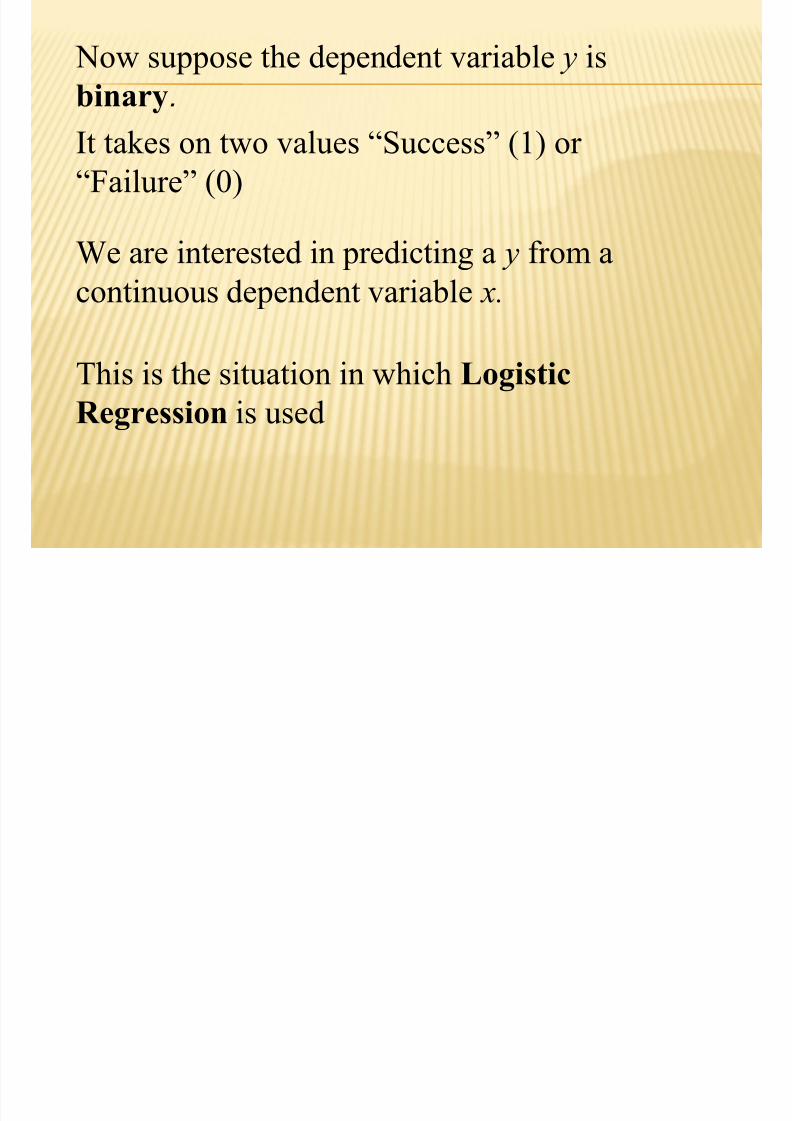
Now suppose the dependent variable y is
binary

7/30/2019 Basic Econometrics Health
http://slidepdf.com/reader/full/basic-econometrics-health 151/183
binary.
It takes on two values “Success” (1) or “Failure” (0)
This is the situation in which Logistic
Regression is used
We are interested in predicting a y from a
continuous dependent variable x.
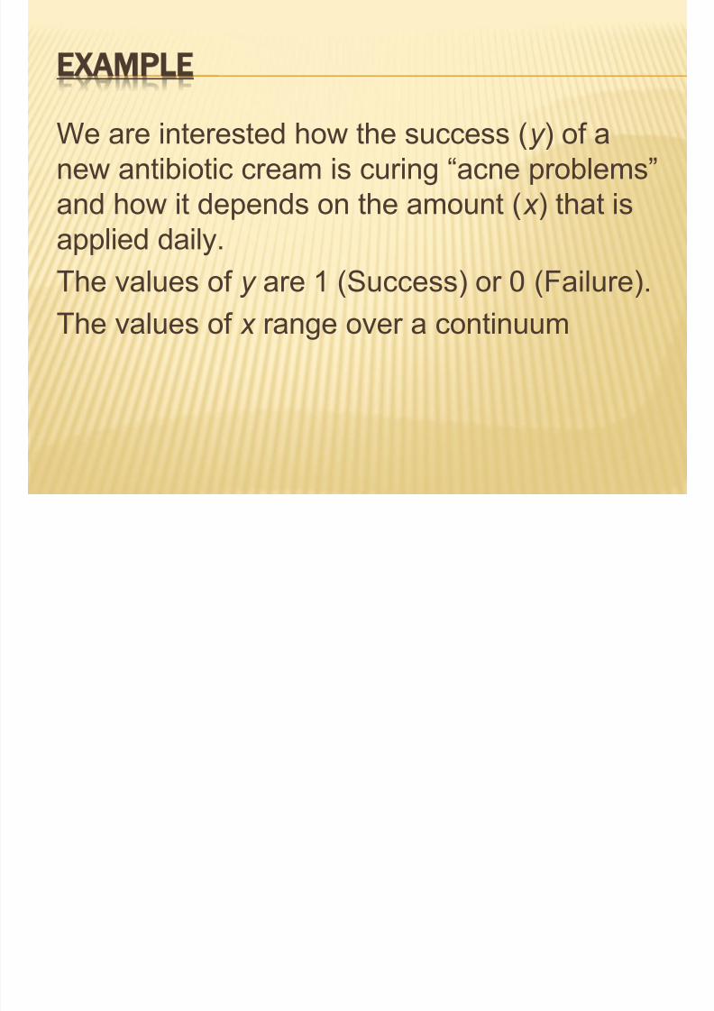
EXAMPLE

7/30/2019 Basic Econometrics Health
http://slidepdf.com/reader/full/basic-econometrics-health 152/183
We are interested how the success (y ) of anew antibiotic cream is curing “acne problems”
and how it depends on the amount ( x ) that is
applied daily.The values of y are 1 (Success) or 0 (Failure).
The values of x range over a continuum
THE LOGISITIC REGRESSION MODEL

7/30/2019 Basic Econometrics Health
http://slidepdf.com/reader/full/basic-econometrics-health 153/183
Let p denote P [y = 1] = P [Success].
This quantity will increase with the value of
x.
1
p
p
The ratio: is called the odds ratio
This quantity will also increase with the value of
x, ranging from zero to infinity.
The quantity: ln1
p p
is called the log odds ratio
EXAMPLE: ODDS RATIO, LOG ODDS
RATIO

7/30/2019 Basic Econometrics Health
http://slidepdf.com/reader/full/basic-econometrics-health 154/183
Suppose a die is rolled:
Success = “roll a six”, p = 1/6
1 16 6
516 6
1
1 1 5
p
p
The odds ratio
1
ln ln ln 0.2 1.690441 5
p
p
The log odds ratio
THE LOGISITIC REGRESSION MODEL

7/30/2019 Basic Econometrics Health
http://slidepdf.com/reader/full/basic-econometrics-health 155/183
0 1
1
x p
e p
i. e. :
In terms of the odds ratio
0 1ln
1
p x
p
Assumes the log odds ratio is linearlyrelated to x.
THE LOGISITIC REGRESSION MODEL

7/30/2019 Basic Econometrics Health
http://slidepdf.com/reader/full/basic-econometrics-health 156/183
0 1
1
x pe
p
or
Solving for p in terms x.
0 1 1 x p e p
0 1 0 1 x x p pe e
0 1
0 11
x
x
e p
e
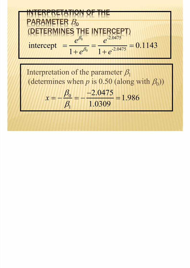
INTERPRETATION OF THE PARAMETER B 0(DETERMINES THE INTERCEPT)

7/30/2019 Basic Econometrics Health
http://slidepdf.com/reader/full/basic-econometrics-health 157/183
0
0.2
0.4
0.6
0.8
1
0 2 4 6 8 10
p
0
0
1
e
e
x
INTERPRETATION OF THE PARAMETER B 1(DETERMINES WHEN P IS 0.50 (ALONG WITH
B0))

7/30/2019 Basic Econometrics Health
http://slidepdf.com/reader/full/basic-econometrics-health 158/183
B 0))
0
0.2
0.4
0.6
0.8
1
0 2 4 6 8 10
p0 1
0 1
1 1
1 1 1 2
x
x
e p
e
x
00 1
1
0 or x x
when
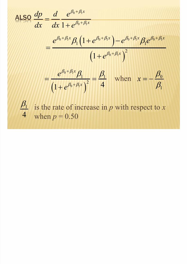
ALSO0 1
0 11
x
x
dp d e
dx dx e
7/30/2019 Basic Econometrics Health
http://slidepdf.com/reader/full/basic-econometrics-health 159/183
1dx dx e
0
1
x
when
0 1 0 1 0 1 0 1
0 1
1 1
2
1
1
x x x x
x
e e e e
e
0 1
0 1
1 1
241
x
x
e
e
1
4
is the rate of increase in p with respect to x
when p = 0.50
INTERPRETATION OF THE PARAMETER B 1(DETERMINES SLOPE WHEN P IS 0.50 )

7/30/2019 Basic Econometrics Health
http://slidepdf.com/reader/full/basic-econometrics-health 160/183
0
0.2
0.4
0.6
0.8
1
0 2 4 6 8 10
p
x
1slope4
THE DATA

7/30/2019 Basic Econometrics Health
http://slidepdf.com/reader/full/basic-econometrics-health 161/183
The data will for each case consist of
1. a value for x, the continuous independent
variable
2. a value for y (1 or 0) (Success or Failure)
Total of n = 250 cases
case x y230 4.7 1
231 0.3 0
232 1.4 0
case x y
1 0.8 0
2 2.3 1
3 2 5 0

7/30/2019 Basic Econometrics Health
http://slidepdf.com/reader/full/basic-econometrics-health 162/183
233 4.5 1
234 1.4 1235 4.5 1
236 3.9 0
237 0.0 0
238 4.3 1
239 1.0 0
240 3.9 1
241 1.1 0
242 3.4 1
243 0.6 0
244 1.6 0
245 3.9 0246 0.2 0
247 2.5 0
248 4.1 1
249 4.2 1
250 4.9 1
3 2.5 0
4 2.8 1
5 3.5 16 4.4 1
7 0.5 0
8 4.5 1
9 4.4 1
10 0.9 011 3.3 1
12 1.1 0
13 2.5 1
14 0.3 1
15 4.5 1
16 1.8 0
17 2.4 1
18 1.6 0
19 1.9 1
20 4.6 1
ESTIMATION OF THE PARAMETERS

7/30/2019 Basic Econometrics Health
http://slidepdf.com/reader/full/basic-econometrics-health 163/183
The parameters are estimated by Maximum
Likelihood estimation and require a
statistical package such as SPSS
USING SPSS TO PERFORM LOGISTIC REGRESSION
O th d t fil

7/30/2019 Basic Econometrics Health
http://slidepdf.com/reader/full/basic-econometrics-health 164/183
Open the data file:
Choose from the menu:
Analyze -> Regression -> Binary Logistic

7/30/2019 Basic Econometrics Health
http://slidepdf.com/reader/full/basic-econometrics-health 165/183
The following dialogue box appears

7/30/2019 Basic Econometrics Health
http://slidepdf.com/reader/full/basic-econometrics-health 166/183
Select the dependent variable ( y) and the independent
variable ( x) (covariate).
Press OK .
Here is the output

7/30/2019 Basic Econometrics Health
http://slidepdf.com/reader/full/basic-econometrics-health 167/183
The Estimates and their S.E.
THE PARAMETER ESTIMATES

7/30/2019 Basic Econometrics Health
http://slidepdf.com/reader/full/basic-econometrics-health 168/183
SEX 1.0309 0.1334
Constant -2.0475 0.332
1 1.0309
0 -2.0475

7/30/2019 Basic Econometrics Health
http://slidepdf.com/reader/full/basic-econometrics-health 169/183

7/30/2019 Basic Econometrics Health
http://slidepdf.com/reader/full/basic-econometrics-health 170/183
Another interpretation of the parameter 1
1
4
is the rate of increase in p with
respect to x when p = 0.50
1 1.03090.258
4 4
The Logistic Regression Model

7/30/2019 Basic Econometrics Health
http://slidepdf.com/reader/full/basic-econometrics-health 171/183
The dependent variable y is binary.
It takes on two values “Success” (1) or
“Failure” (0)
We are interested in predicting a y from a
continuous dependent variable x.
THE LOGISITIC REGRESSION MODEL
7/30/2019 Basic Econometrics Health
http://slidepdf.com/reader/full/basic-econometrics-health 172/183
Let p denote P [y = 1] = P [Success].
This quantity will increase with the value of
x.
1
p
p
The ratio: is called the odds ratio
This quantity will also increase with the value of
x, ranging from zero to infinity.
The quantity: ln1
p p
is called the log odds ratio
THE LOGISITIC REGRESSION MODEL

7/30/2019 Basic Econometrics Health
http://slidepdf.com/reader/full/basic-econometrics-health 173/183
0 1
1
x p
e p
i. e. :
In terms of the odds ratio
0 1ln
1
p x
p
Assumes the log odds ratio is linearlyrelated to x.
THE LOGISITIC REGRESSION MODEL

7/30/2019 Basic Econometrics Health
http://slidepdf.com/reader/full/basic-econometrics-health 174/183
In terms of p
0 1
0 11
x
x
e p
e
THE GRAPH OF P VS X

7/30/2019 Basic Econometrics Health
http://slidepdf.com/reader/full/basic-econometrics-health 175/183
0
0.2
0.4
0.6
0.8
1
0 2 4 6 8 10
p0 1
0 11
x
x
e
p e
x

7/30/2019 Basic Econometrics Health
http://slidepdf.com/reader/full/basic-econometrics-health 176/183
THE MULTIPLE LOGISTIC REGRESSIONMODEL
Here we attempt to predict the outcome of
bi i bl Y f l

7/30/2019 Basic Econometrics Health
http://slidepdf.com/reader/full/basic-econometrics-health 177/183
a binary response variable Y from several
independent variables X 1, X 2 , … etc
0 1 1ln 1 p p
p
X X p
0 1 1
0 1 1or 1
p p
p p
X X
X X
e
p e

7/30/2019 Basic Econometrics Health
http://slidepdf.com/reader/full/basic-econometrics-health 178/183
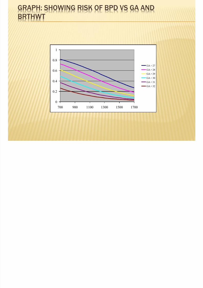
For n = 223 infants in prenatal ward thefollowing measurements were determined

7/30/2019 Basic Econometrics Health
http://slidepdf.com/reader/full/basic-econometrics-health 179/183
following measurements were determined
1. X 1 = gestational Age (weeks),
2. X 2 = Birth weight (grams) and
3. Y = presence of BPD
THE DATAcase Gestational Age Birthweight presence of BMD
1 28.6 1119 1
2 31.5 1222 0
3 30.3 1311 1
4 28.9 1082 0
5 30 3 1269 0

7/30/2019 Basic Econometrics Health
http://slidepdf.com/reader/full/basic-econometrics-health 180/183
5 30.3 1269 0
6 30.5 1289 0
7 28.5 1147 08 27.9 1136 1
9 30 972 0
10 31 1252 0
11 27.4 818 0
12 29.4 1275 0
13 30.8 1231 0
14 30.4 1112 0
15 31.1 1353 1
16 26.7 1067 1
17 27.4 846 1
18 28 1013 0
19 29.3 1055 0
20 30.4 1226 0
21 30.2 1237 0
22 30.2 1287 0
23 30.1 1215 0
24 27 929 1
25 30.3 1159 0
26 27.4 1046 1
THE RESULTS
Variables in the Equation
003 001 4 885 1 027 998BirthweightStep
B S.E. Wald df Sig. Exp(B)

7/30/2019 Basic Econometrics Health
http://slidepdf.com/reader/full/basic-econometrics-health 181/183
ln 16.858 .003 .5051
p
BW GA p
-.003 .001 4.885 1 .027 .998
-.505 .133 14.458 1 .000 .604
16.858 3.642 21.422 1 .000 2.1E+07
Birthweight
GestationalAge
Constant
Step
1a
Variable(s) entered on step 1 : Birthweight, GestationalAge.a.
16.858 .003 .505
1
BW GA pe
p
16.858 .003 .505
16.858 .003 .5051
BW GA
BW GA
e p
e
GRAPH: SHOWING RISK OF BPD VS GA ANDBRTHWT

7/30/2019 Basic Econometrics Health
http://slidepdf.com/reader/full/basic-econometrics-health 182/183
0
0.2
0.4
0.6
0.8
1
700 900 1100 1300 1500 1700
GA = 27
GA = 28
GA = 29
GA = 30
GA = 31
GA = 32

7/30/2019 Basic Econometrics Health
http://slidepdf.com/reader/full/basic-econometrics-health 183/183
NON PARAMETRIC STATISTICS