basic di usion tensor imaging - university of california,...

28 Basic Di↵usion Tensor Imaging

28.1 Introduction

1

Let us pause here for a moment and review what has been learned so far. In Chapter 14 wesaw how an NMR signal can be generated and detected from a sample within a coil. We thenelaborated on this idea in two di↵erent, and to this point, unconnected, ways. The first was todemonstrate (Chapter 16) that localization of the signal from di↵erent spatial regions of thesample could be achieved by the application of magnetic field gradients and reconstruction byFourier transformation. This is the process of magnetic resonance imaging (MRI). We extendedthese ideas to ultrafast (single shot) imaging in Chapter 18, such as echo planar imaging (EPI),that allowed us to acquire images rapidly enough to obviate bulk subject motion, at the expenseof greater sensitivity to a number of physical e↵ects that create artifacts, that we nonethelesscould mitigate. But we also reconsidered the simple case of a sample in a coil in the presenceof a bipolar gradient pulse and discovered (Chapter 25) that di↵using spins produced a signalloss due to their motion through the gradients. Moreover, with an appropriate model for thedi↵usion process, the di↵usion tensor could be estimated, from which we could derived scalarmeasures related to the mean di↵usivity and the di↵usion anisotropy. The bipolar pulse had theadditional feature that it refocused stationary spins at its completion. In the present chapter weare going to tie this all together for the following purpose: To combine the di↵usion weightingand subsequent analysis we examined for a small sample with the spatial localization (MRI)on a full human brain in order to produce images with di↵usion weighting from which can beperformed localized (e.g. in every voxel) estimation of the di↵usion tensor. This entire process iscalled di↵usion tensor imaging , or DTI .

As mentioned in the Introduction and in Chapter 25, the order I’ve chosen to present theaformentioned aspects of this process is somewhat non-standard, and at first glance perhapseven disconnected. But that is precisely the point. The payo↵ comes here in this chapter wherewe see that the process of DTI is really just the combination of several experimental proceduresand physical processes that stand on their own. These distinctions are important to grasp becauseone of the biggest hurdles I’ve encountered in teaching DTI is the confusion over what aspectsare related to di↵usion, which are related to imaging, and which are related to reconstruction andestimation. This motivated the presentation in terms of the separated components to be combinedonly after each is understood in its own right. The central fact that allows this simplification isthat bipolar gradients a↵ect di↵using spins but leave stationary spins unchanged. As we shallsee, this allows us to really just combine the results of these aformentioned chapters into one

1 Make it clear here that you’re just looking at the single fiber voxel model, etc, etc.


procedure. And the pleasing result is that this central chapter is relatively short: you have allthe background you need to understand how DTI works.

Now, having said that, we still must proceed with caution, and state from the outset that ourgoal in this chapter is to describe the most basic form of DTI. By “basic” we mean specifically:2

• The di↵usion is assumed to be Gaussian• There is no subject movement• Di↵usion gradients cause no distortions• Di↵usion through imaging gradients has no e↵ect

In later chapter we will relax these restrictions and consider important extensions to DTI thatare necessary to more accurately characterize complex neural tissues.

28.2 Di↵usion in a bipolar gradient: Review

In the previous chapter we investigated the e↵ect of di↵usion in a bipolar gradient, the resultsof which we review here. We found that a bipolar gradient rephased all of the stationary spins,causing a gradient echo. But this required that the spins be stationary because the rephasingrequired that the spins were subject to an equal and opposite gradient induced field. Since thisfield is spatially dependent, by definition, any movement of a spin would cause it to have amismatch between the magnitude of its starting and ending phases, and thus we would expectthat the total signal, no longer being from spins completely in phase, would be reduced. This isprecisely the e↵ect produced by di↵using spins: since their final location is di↵erent from theirinitial location, their phases are di↵erent, and thus all the spins no longer come back into phaseand the final signal is reduced. How much the signal is reduced depends on how much theygo out of phase, which depends on the particulars of their motion. Since it is impractical (ney,impossible) to follow the trajectory of individual spins, we must resort to probabilistic arguments.

So, in order to determine the signal in the presence of moving spins, we need to know where theystart and where they end up, and then figure out the phase they’ve accrued by changing locationsboth in the presence of the gradients (i.e., during the time �) as well as what happens in thetime � between the centers of the gradients (i.e., the area/2). This problem sounds complicated.But what is remarkable is that, at least for the most basic case, the answer to these questionsis surprisingly simple. We’ll give a sketch of the answer here, and then go into the details in therest of the chapter about how we arrived at this, what assumption were needed, and then touchon where those assumptions fail. The details of that will have to wait for a later chapter.

Let us return to our simple model of Gaussian di↵usion. Recall the meaning of the Gaussiandistribution that characterizes di↵usion: it is the probability of finding a spin at a particularlocation after a certain time. This is just what we require in order to determine what locationchanges, and hence what phase changes, are accrued during the bipolar pulse. The answer, as weshall see, is that the signal decays in a very simple way as a function of the applied gradients,whose amplitudes and parameters are contained within a parameter b, called the b-factor . Foran anisotropic tissue characterized by Gaussian di↵usion with a di↵usion tensor D, we foundthat the signal in the presense of a bipolar gradient characterized by the b-factor is (Eqn ??)

s(q, ⌧) = e�b

˜

D (28.1)

2 Have we listed all our implicit assumptions of this chapter?

28.3 Creating di↵usion contrast in images: Di↵usion Weighting Gradients 509

where s ⌘ s(b)/so

is the ratio of the di↵usion weighted signal to the unweighted (i.e., b = 0)signal s

o

⌘ s(b = 0). The b-factor is given by

b = q2⌧ (28.2)

where q ⌘ |q| is just the area of the gradient that is pointing along the q direction (Eqn ?? ) and

D ⌘ q

t

Dq (28.3)

is the projection of the di↵usion tensor D along the direction q.So the sensitivity of the bipolar gradient to di↵usion depends upon the area squared: doubling

the gradient amplitude quadruples the di↵usion sensitivity. Note also that if the gradient is turnedo↵ (G = 0), then b = 0 and s(b) = s

o

. So turning o↵ the gradient pulse gives us the constant so

.The decay is also proportional to the time ⌧ , often called the di↵usion time, which is given by

⌧ = � � �/3 (28.4)

and so is proportional to the time �, minus a term proportional to the gradient width. Thusputting the gradients farther apart increases the sensitivity. This makes sense, since the longerspins are allowed to di↵use, the greater the spread in their locations, thus the greater the vari-ations in the fields they subject to, and thus the wider the spread of phases, and thus the moresignal loss when they’re all added up.

And, because the di↵usion tensor represents variations in the di↵usion along di↵erent spatialdirections, this decaying exponential characteristic of the signal depends upon which directionwe measure the di↵usion along. That is, which direction the di↵usion weighting is along. Wefound, using the vectorial nature of gradients, that it was a simple matter to point the di↵usionweighting along any desired direction by suitable combination of bipolar gradients along the threeprincipal axes of the scanner. Performing measurements along di↵erent directions and using ourmodel for the di↵usion process, it was then possible to estimate the di↵usion tensor.

Let us now turn to extending this to the imaging process. The key new feature is the incorpo-ration of the di↵usion weighting gradient into an imaging sequence.

28.3 Creating di↵usion contrast in images: Di↵usion Weighting Gradients

We now come to an important juncture in the book. We saw in Chapter 16 how to create MRimages, and in Chapter 25 how the bipolar gradient causes a signal intensity that is proportionalto di↵usion. How can we then proceed to the real work of this book, which is to combine thetwo to get di↵usion weighted images? Given the complicated sequence of RF and gradient pulsesnecessary to form a complete MR image, this might seem like a daunting task. But, surprisingly,this is not so! And all because of the nice qualities of the bipolar gradient pulse (recall that weuse this term as a shorthand to refer specifically to two gradients of equal areas and oppositesign). Recall the two essential properties of the bipolar gradient pulse: 1) Stationary spins arerefocussed at the end of the second pulse; 2) Di↵using spins su↵er a signal loss proportional tothe amplitude and timing of the two pulses. From these two facts alone we can develop the basicmethod of DTI. Because a bipolar gradient refocussing stationary spins, it can be inserted intoa pulse sequence, as long as it doesn’t interfere (i.e., overlap) with any of the imaging gradients,and be invisible to the imaging portion of the pulse sequence! And so, from fact (2), we can


⌧

d d

D

»g x»

TEê2 TEê2

e

»g y»

90° 180° echo

Gx

Gy

Gz

DAQ

(a) Spin echo EPI acquisition.

⌧

d d

D

»g x»

TEê2 TEê2

e

»g y»

90° 180° echo

Gx

Gy

Gz

DAQ

(b) Di↵usion weighted spin echo EPI acquisi-

tion.

Figure 28.1 Spin echo EPI di↵usion weighted pulse sequence. Bipolar di↵usion weighting gradient pulses

(gray lobes) are inserted into a basic spin echo EPI pulse sequence without interfering with the imaging

process because a bipolar pulse refocusses stationary spins and is thus invisible to the pulse sequence

as long as it does not overlap with the imaging gradients.

add bipolar di↵usion weighting gradients whose amplitudes and timings we can manipulate toprobe the di↵usion characteristics of our tissue, but create MR images simultaneously. The resultis MR images that have di↵usion weighting everywhere, ie, in each voxel, thus allowing us toinvestigate the spatial variations of whatever di↵usion related quantities we can measure withina voxel. Such images are called di↵usion weighted images .

The most straightforward, and most common, method of combining di↵usion weighting withand imaging sequences is to insert a bipolar pair of di↵usion weighting gradients into a standardspin echo pulse sequence, as shown in Figure 28.1.

Note the important fact that the second lobe of the di↵usion gradients in Figure 28.1 is thesame sign as the first lobe because of the presence of the 180� refocussing pulse This has beenimplicit in our previous description of ”e↵ective gradients” (Section ??), in which we replace twogradient on either side of the 180� pulse with a bipolar pair. This allowed us to discuss di↵usione↵ects without having to mention and RF pulses. Throughout what follows we will ignore thee↵ects of the refocussing pulse(s). In practice, we have to be careful about where these di↵usionweighting gradients are placed in the pulse sequence, and what system imperfections they aresubject to. These will be discussed in detail in later chapters.

Notice the important fact that the di↵usion weighting gradients are applied independently oneach axis in Figure 28.1. That is, the second lobe of the bipolar gradient on the x-axis refocussesspins brought out of phase by the first lobe on the x-axis, regardless of what’s happening onthe y and z axes. So the bipolar gradients on each of the axes refocus stationary spins on theirrespsective axes, and produce di↵usion weighting along these axes as well, independently of whathappens on the other axes. But now recall the important and very practical fact that gradients

add like vectors. Therefore, we see that the combined e↵ect of simultaneously applied di↵usion

weighting gradients is the rotation of the direction of di↵usion sensitivity in the direction defined

by the resulting combined gradient vector. This was shown in Figure 29.1. Since we, the systemoperator, controls these gradients, we can point them in any directions we want. For example, inFigure 28.5 is shown di↵usion encoding along the three principal scanner axes and an arbitrarydirection.

So now we combine these ideas - bipolar di↵usion weighting gradient put into a spin echo

28.4 Interlude: What is the e↵ect of the imaging gradients? 511

(a) Di↵usion weighting parallel to theright splenium of the corpus callosum.

(b) Di↵usion weighting parallel to the leftsplenium of the corpus callosum.

Figure 28.2 (Use newer images!) Two images with di↵usion weighting in di↵erent directions (shown

by the green arrows) approximately parallel and perpendicular to the left and right splenia of the

corpus callosum. This example was specifically chosen because the two structure are close to

perpendicular, so the two chosen gradient directions applied along these structures are close to

perpendicular to one another. In both cases, there is signal loss in the portion of the corpus callosum

parallel to the applied gradient, but not that perpendicular to it (white arrows).

sequence with our ability to di↵usion encode in di↵erent directions, and see what happens. InFigure 28.2 is shown two images with di↵usion sensitivity along two di↵erent directions chosen tobe along the right and left splenia of the corpus callosum. This example was specifically chosenbecause the two structure are close to perpendicular, so the two chosen gradient directions appliedalong these structures are close to perpendicular to one another. In both cases, there is signal lossin the portion of the corpus callosum parallel to the applied gradient, but not that perpendicularto it (white arrows).

28.4 Interlude: What is the e↵ect of the imaging gradients?

If di↵usion through gradients results in a directionally dependent signal loss, don’t the imag-ing gradients have some e↵ect? In fact, they do, but in most clinical applications this e↵ect isnegligible. That is not the case is high field imaging using high powered gradients, however. Tounderstand the e↵ect of imaging gradients, it is useful to look at the di↵usion weighting processin a di↵erent way.

In the simple case of Gaussian di↵usion, the spread of spins in the spatial domain is equivalentto a convolution in the image domain by a Gaussian kernel. This is shown schematically inFigure 28.3 for the 1D case. As we saw in Section 11.5, convolution of the two functions I(x)and H(x) is one domain (x) is equivalent to multiplication of their Fourier transforms I(k) andH(k) in the conjugate domain:

I(x) ? H(x) = I(k)H(k) (28.5)


✶

a zillion spins

t = 0 t = ⌧

τ

(a) A group of spins at time t = 0 spreads into a Gaussian distribution at time t = ⌧ witha standard deviation � =

p2D⌧ .

✶

a zillion spins

t = 0 t = ⌧

τ

(b) The process in (a) is equivalent to convolution of the initial distribution with a Gaussian

with standard deviation � =p2D⌧ .

Figure 28.3 Gaussian di↵usion is equivalent to convolution in the image domain.

where ”” denotes the Fourier transform. In this case x is the spatial (image) domain and k is thefourier (data acquisition) domain. Let I(x) denotes the image and H(x) the convolving kerneldue to di↵usion. Because the width of Gaussian convolution kernel H(x) is very small comparedto the voxel dimensions (⌧ = 100 ms ! � ⇡ 15 µm), its Fourier transform H(k) is very broadwith respect to the k-space data I(k). This is illustrated in Figure 28.4 Because the width ofH(x) is very small, its Fourier tranform H(x) (the red curve in Figure ??) is very broad. Theresult is that small gradients (e.g., imaging gradients on a typical 3T clinical system) producelittle di↵usion e↵ect and much larger di↵usion weighting gradients that shift the center of k-spacetoward the edge of H(x) are needed to produced a measureable e↵ect. This is not necessarilytrue on high field high performance systems where the imaging gradients can be quite large.3

28.5 The spatial variations of the di↵usion attenuation

Now that we have seen that the imaging process can be integrated with the di↵usion weightingprocess (which consists of bipolar di↵usion weighting gradients on each axis), the question, finally,is “What is the signal attenuation in each voxel?”. Well, for our simple model of di↵usion asunrestricted (free) Gaussian, we already know the answer to this, and with a slight addition

3 Give examples of gradient values at 3T and on, say, and 11.7T system.

28.5 The spatial variations of the di↵usion attenuation 513

FT

k

�� FOV = 24 cm �!

FT

b=0

FT

DWI

� ⇡ 15µm � voxel dimensions

>> image k-space dimensions

e�x

2/D dt � e�k

2D dt

Figure 28.4 Convolution of the image by the di↵usion kernel H(x) is equivalent to multiplication of the

data by the Fourier transform of the di↵usion kernel. Because the width of H(x) is very small, its

Fourier tranform

˜H(x) (red) is very broad. The result is that small (e.g., imaging) gradients produce

little di↵usion e↵ect and much larger di↵usion weighting gradients that shift the center of k-spacetoward the edge of

˜H(x) are needed to produced a measureable e↵ect.

to our notation we can make it obvious. The signal attenuation in 3-dimensions from a bipolardi↵usion weighting gradient is given by Eqn 27.3. This is the signal model for a voxel so is easilyextended to express the spatial variation of the di↵usion in the entire image, the distribution ofintensities in three dimensional space x = {x, y, z} is

s(x, b) = s0

(x) e�b

˜

D(x) + ⌘(x, b) (28.6)

where D ⌘ u

T ·D ·u is the projection of the di↵usion tensor along the applied di↵usion weightinggradient direction u, b = q2⌧ = g2�2 (� � �/3) is the b-factor, and where ⌘(x, b) is the noise ands0

(x) is image acquired without di↵usion weighting but all other timing parameters the sameas in the di↵usion weighted images. This is important because the relaxation contrast, whichdepends on the timing parameters, must be the same in s(x, 0) as in the di↵usion weightedimages in order that they are normalized correctly so that signal loss due to T

2

relaxation is notconfounded with that from di↵usion weighting (see the discussion surrounding m

0

in Eqn ??).The image s(x, 0) is often referred to as the ”b equals zero” image. Now, di↵usion weightedsequences typically have long echo times TE in order to accommodate the di↵usion weightinggradients. An image s(x, 0) acquired with the same timing parameters but without di↵usionweighting gradients will thus tend to be T

2

�weighted (see Chapter 17). The image s0

(x) is thusalso often referred to as the ”T

2

” image. The noise ⌘(x, b) is generally spatially varying, althoughwe will simplify it by assuming that it is not: ⌘(b) = ⌘(x, b).


The application of di↵usion weighting gradients therefore produces a spatial pattern of signalattenuation throughout the image concomitant with the spatial distribution of di↵usion tensorsD(x). In this chapter we will treat each of the voxels as independent, so that we reconstructthe di↵usion tensor in each voxel without any reference to its neighbors. Thus in this section wewill figure out what we need to do to reconstruct D and then just repeat the procedure for eachvoxel. This is again the procedure in standard DTI. Later, in Chapter 40 we will be concernedwith the spatial relationship of the di↵usion in the voxels and then we’ll have to consider thefact that the local di↵usion tensor is really a component of a more spatially extended di↵usionfield.

The noise ⌘(x, b) is assumed to be Gaussian with zero mean and variance �2

⌘

: that is ⌘(x, b) ⇠N(0, �2

⌘

), because, as we found in Chapter 19, this is a good model for the background noisein MR images. This, of course, is predicated on using the complex MR images, rather than themagnitude images, which have noise that is characterized by a Rayleigh, (?), rather than a Gaus-sian, distribution (Chapter 19) 4. It is common practice, however, to use the magnitude images,which means that the assumption of Gaussian noise is incorrect. This will become important forlow SNR experiments, such as those using high b-values, where the noise becomes comparableto the signal.

Another implicit assumption in the modeling of ⌘(x, b) as Gaussian is that all other noisesources that are not thermal have been eliminated. In practice, to perform an experiment preciselyenough to make this statement even approximately true is a non-trivial a↵air. Su�ce it to sayfor now that the largest sources of error in DTI or not thermal noise, but eddy currents andfield distortions. We will return to this issue in Chapter 30 where we demonstrate the practicalnecessity of reducing these artifacts and show some methods by which this can be accomplishedto a reasonable degree.

It is important that the di↵usion weighting gradients in Figure 28.1 along each imaging axisdo not overlap the imaging gradients or they would interfere with the imaging process5. Butthe di↵usion gradients on each axis can be applied simultaneously, and in fact this is of criticalimportance. For, just as in imaging, gradient fields add as vectors so that combinations of simul-taneously applied di↵usion weighting gradients along the magnet’s {x, y, z} coordinates can beused to make the net di↵usion weighting gradient occur in any direction. An example of s

0

(x)and some di↵usion weighted images along di↵erent directions is shown Figure 28.5. Notice thatthe gradient directions are defined in terms of the unit vectors u. For the same timing parametersand gradient strength, the b � value remains the same, although the direction of the di↵usionsensitivity changes. The family of the endpoints of all arrow that are of constant length butarbitrary orientation form the surface of a sphere. Therefore, the surface of possible di↵usiongradient vector endpoints for a constant b-value but arbitrary direction is a sphere. This is calledthe di↵usion sampling sphere, and depicted in Figure 28.5(k). From this week see also that thelength of the vector, and thus the sphere’s radius, is the b-value. Thus sampling spheres for dif-ferent b� values are thus concentric spheres. Here again is another system for which is naturallydescribed by a spherical coordinate system (Section 2.3).

4 need discussion of Rayleigh (or is it Riccian?) noise in MRI!5 For gradient/imaging cross term interactions, see Mattielo refs in the Basser, Jones NMR in Biomedicine

review.

28.6 Displaying the estimated tensor 515

t

Gz

t

Gy

t

Gx

(f) g = 0

t

Gz

t

Gy

t

Gx

(g) gx

= G

x

ux

.

t

Gz

t

Gy

t

Gx

(h) gy

= G

y

uy

.

t

Gz

t

Gy

t

Gx

(i) gz

= G

z

uz

.

t

Gx

t

Gy

t

Gz

(j) gx,y,z

= G · u5.

x

y

z

x

y

z

x

y

z

x

y

z

x

y

z

(k) Gradient directions and the sampling sphere.

Figure 28.5 Directional di↵usion encoding. (Top row) Di↵usion weighted images EPI images at 3T with

b = 2000s/mm2; (Second row) Di↵usion gradients used in (a-e); (Bottom) Corresponding di↵usion

gradient directions in (f-j). (Collect correct images!). Gx

, Gy

, and Gz

are the amplitudes of the x,y, and z gradients and G = {G

x

, Gy

, Gz

}.

28.6 Displaying the estimated tensor

There are several display methods that are particularly useful in visualizing the local structureof di↵usion. As we saw in Section 27.2, estimation of the di↵usion tensor is tantamount to recon-structing the 3D Gaussian pdf, from which can be constructed the contours of the probabilitydistribution of particle positions: the di↵usion ellipsoids. This can be calculated in each voxel,since the di↵usion tensor is estimated in each voxel, and displayed as an image, as in Figure 28.6.This method of presentation is useful not only in allowing us to quickly assess the di↵usion char-acteristics of individual voxels, but also to give a more global picture of the patterns of di↵usionamongst voxels. We’ll follow this line of thought in the next section.

(This next figure was in adv-hard.tex for some reason. I moved it here but need

text.)

An example in human data is shown in Figure 28.7.


Figure 28.6 The reconstructed di↵usion ellipsoids in a selected region of the brain.

Figure 28.7 The estimated di↵usion ellipsoids in a normal human brain. Note that the largest are in

regions of CSF, which has the highest mean di↵usivity. The anisotropy, on the other hand (shown in

underlay in the form of the FA) accentuates the white matter, where it is largest.

28.7 Parameter maps

We have seen that the basic DTI method combines the results of Chapter 25 with the imagingmethods of Chapter 18 to acquire data that is di↵usion weighted along multiple directions. InChapter 29 we saw how to estimate the di↵usion tensor from this data. The beauty of MRIprocess is that the result of combining these operations is that we can now perform the same

analysis we did in Chapter 29 for a single sample in each voxel. That is, we can essentially treat

28.7 Parameter maps 517

(a) axial (c) coronal(b) sagittal(a) Axial(a) axial (c) coronal(b) sagittal(b) Sagittal(a) axial (c) coronal(b) sagittal (c) Coronal

Figure 28.8 Anatomical images from a normal human subject shown at three orthogonal orientations.

inversion recovert T1-weighted 3D fast spoiled gradient recalled echo pulse sequence with parameters:

flip angle ↵ = 12

�, echo time TE = 3ms, repetition time TR = 8ms, matrix size =

(RL,AP, IS) = (172⇥ 256⇥ 256), field of view FOV = (170⇥ 240⇥ 240)mm for a resolution of

(1⇥ .938⇥ .938)mm. (Data courtesy of Dr Susan Tapert, UCSD.)

each voxel as an individual sample, and follow that analysis procedure outlined in Chapter 29.Specifically, once the gradient directions are specified, and the b-matrix constructed, the data ineach voxel are fit to a model. For the Gaussian model, we simply plug in the data in each voxelto a routine such as AFNI’s 3dDWItoDT which does a non-linear fit for the di↵usion tensorunder the assumption of additive, Gaussian noise, returning the eigenvalues and eigenvectors.The eigenvalues will tell us about the magnitude of the di↵usion along the principal directionsof the di↵usion ellipsoid, as defined by the eigenvectors. Mathematically,

D

"measured

=

R

t

"eigenvectors

D⇤

"eigenvalues

R

"eigenvectors

(28.7)

Having determined the eigensystem (i.e., the eigenvalues and eigenvectors) in each voxel from themeasured di↵usion tensor, we can then do several important things. First, we can create the mapsof the di↵usion magnitude parameters, such as the mean di↵usivity and the fractional anisotropy,from the eigenvalues. We can also look at the direction of maximum di↵usivity from the largesteigenvector, which should tell us something about the underlying structure. And from both theeigenvalues and the eigenvectors we can reconstruct the di↵usion ellipsoid or, equivalently, andestimate of the measured apparent angular di↵usion coe�cient (i.e., the “shape” of di↵usion wediscussed in Section 27.4). We’ll consider each of these in order in the next sections.

We can now apply to each voxel the procedures for estimation of the di↵usion tensor discussionin the last chapter. From the eigenvalues in each voxel we can calculate the mean di↵usivity D

and the fractional anisotropy and make images of those parameters. These are shown for a set ofdata collected on a normal human brain at 3T whose anatomical images are shown in Eqn 28.8.The mean di↵usivity and the fractional anisotropy in each voxel of a di↵usion tensor image isshown in Figure 28.9. A very useful way to display this information is to overlay the parametersin color over the high resolution anatomical images, displayed in a grayscale. The mean di↵usivityin each voxel of a di↵usion tensor image (Section 29.6) is shown overlayed on the anatomicalimaging in Figure 28.10. An example of the FA calculated from the di↵usion tensor in eachvoxel (Section 29.7) of a di↵usion tensor image is shown overlayed on the anatomical imaging inFigure 28.11. Notice that the area of high mean di↵usivity are in the regions of cerebro-spinal


(a) Axial MD (b) Axial FA

(c) Sagittal MD (d) Sagittal FA

(e) Coronal MD (f) Coronal FA

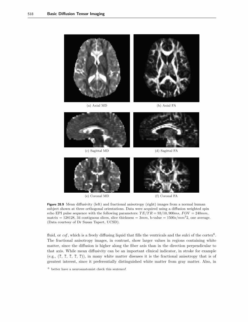
Figure 28.9 Mean di↵usivity (left) and fractional anisotropy (right) images from a normal human

subject shown at three orthogonal orientations. Data were acquired using a di↵usion weighted spin

echo EPI pulse sequence with the following parameters: TE/TR = 93/10, 900ms, FOV = 240mm,

matrix = 128128, 34 contiguous slices, slice thickness = 3mm, b-value = 1500s/mm22, one average.

(Data courtesy of Dr Susan Tapert, UCSD).

fluid, or csf , which is a freely di↵using liquid that fills the ventricals and the sulci of the cortex6.The fractional anisotropy images, in contrast, show larger values in regions containing whitematter, since the di↵usion is higher along the fiber axis than in the direction perpendicular tothat axis. While mean di↵usivity can be an important clinical indicator, in stroke for example(e.g., (?, ?, ?, ?, ?)), in many white matter diseases it is the fractional anisotropy that is ofgreatest interest, since it preferentially distinguished white matter from gray matter. Also, in

6 better have a neuroanatomist check this sentence!

28.8 The direction of di↵usion: The principal eigenvector 519


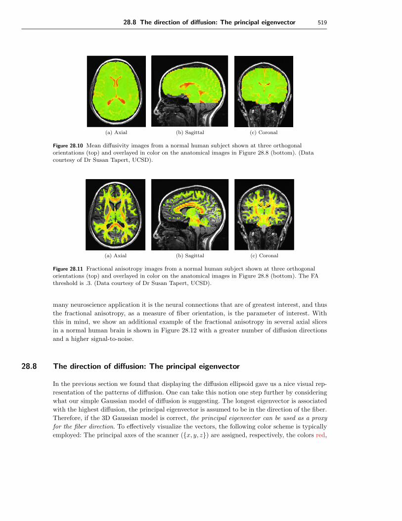
Figure 28.10 Mean di↵usivity images from a normal human subject shown at three orthogonal

orientations (top) and overlayed in color on the anatomical images in Figure 28.8 (bottom). (Data

courtesy of Dr Susan Tapert, UCSD).


Figure 28.11 Fractional anisotropy images from a normal human subject shown at three orthogonal

orientations (top) and overlayed in color on the anatomical images in Figure 28.8 (bottom). The FA

threshold is .3. (Data courtesy of Dr Susan Tapert, UCSD).

many neuroscience application it is the neural connections that are of greatest interest, and thusthe fractional anisotropy, as a measure of fiber orientation, is the parameter of interest. Withthis in mind, we show an additional example of the fractional anisotropy in several axial slicesin a normal human brain is shown in Figure 28.12 with a greater number of di↵usion directionsand a higher signal-to-noise.

28.8 The direction of di↵usion: The principal eigenvector

In the previous section we found that displaying the di↵usion ellipsoid gave us a nice visual rep-resentation of the patterns of di↵usion. One can take this notion one step further by consideringwhat our simple Gaussian model of di↵usion is suggesting. The longest eigenvector is associatedwith the highest di↵usion, the principal eigenvector is assumed to be in the direction of the fiber.Therefore, if the 3D Gaussian model is correct, the principal eigenvector can be used as a proxy

for the fiber direction. To e↵ectively visualize the vectors, the following color scheme is typicallyemployed: The principal axes of the scanner ({x, y, z}) are assigned, respectively, the colors red,


Figure 28.12 Fractional anisotropy in several axial slices in a normal human brain. (Put imaging

parameters here! This is 61 directions!)

green, and blue. An arbitrary vector is assigned a color that is a mixture of these three colors,with the amount of each color determined by the projection of the vector along the principalaxes. For example, a vector at a 45� angle in the x � y is projected equally along the x and y

axes, and thus is assigned half red and half green. The color schemes for each principal planeare shown in Figures 28.13a- 28.13c. An example is shown in Figure 28.13. One di�culty withrepresenting the direction with arrows as in Figure 28.13 is that it if often quite hard to see thesearrows in a full image. For this reason, an popular alternative scheme is to do away with the ar-rows and instead represent the direction of the principal eigenvector in a voxel by the directionalcolor. Voxels with principal eigenvectors pointing along these directions are given these colors.This visualization technique allows one to quickly and easily assess the estimated fiber directionsover an entire image, as is evident from the high resolution rat brain DTI images Figure 28.14.Combining the FA along with the principal eigenvector is also a useful way to combine parametermaps, as shown in Figure 28.15.

28.8 The direction of di↵usion: The principal eigenvector 521

(a) x� y plane

(b) y � z plane

(c) z � x plane(d) The principal eigenvectors overlayed on anatomical scan.

Figure 28.13 Color encoding scheme for principal eigenvectors.

Suggested Reading


⌧⌧

Figure 28.14 Color encoding the of the principal eigenvectors in the principal slices in a high field

(11.7T) DTI data of a rat brain (data courtesy of Dr. J.M. Tyszka, CalTech).

⌧

(a) Axial

⌧

(b) Sagittal

⌧

(c) Coronal

Figure 28.15 Fractional anisotropy and the principal eigenvectors images from a normal human subject

shown at three orthogonal orientations (top) and overlayed in color on the anatomical images in

Figure 28.8 (bottom). The FA threshold is .3. (Data courtesy of Dr Susan Tapert, UCSD.)

basic di usion tensor imaging - university of california,...

Documents