basic control volume - semantic scholar · basic control volume finite element methods for fluids...
TRANSCRIPT


Basic Control Volume Finite Element Methods
for Fluids and Solids

This page intentionally left blankThis page intentionally left blank

N E W J E R S E Y • L O N D O N • S I N G A P O R E • B E I J I N G • S H A N G H A I • H O N G K O N G • TA I P E I • C H E N N A I
World Scientific
Basic Control Volume Finite Element Methods
for Fluids and Solids
Vaughan R VollerUniversity of Minnesota, USA
IISc Research Monographs Series

British Library Cataloguing-in-Publication DataA catalogue record for this book is available from the British Library.
For photocopying of material in this volume, please pay a copying fee through the CopyrightClearance Center, Inc., 222 Rosewood Drive, Danvers, MA 01923, USA. In this case permission tophotocopy is not required from the publisher.
ISBN-13 978-981-283-498-0ISBN-10 981-283-498-2
All rights reserved. This book, or parts thereof, may not be reproduced in any form or by any means,electronic or mechanical, including photocopying, recording or any information storage and retrievalsystem now known or to be invented, without written permission from the Publisher.
Copyright © 2009 by World Scientific Publishing Co. Pte. Ltd.
Published by
World Scientific Publishing Co. Pte. Ltd.
5 Toh Tuck Link, Singapore 596224
USA office: 27 Warren Street, Suite 401-402, Hackensack, NJ 07601
UK office: 57 Shelton Street, Covent Garden, London WC2H 9HE
Printed in Singapore.
BASIC CONTROL VOLUME FINITE ELEMENT METHODS FOR FLUIDSAND SOLIDSIISc Research Monographs Series — Vol. 1
Steven - Basic Control Volume.pmd 11/24/2008, 10:04 AM1
A-PDF Merger DEMO : Purchase from www.A-PDF.com to remove the watermark

v
Series Preface
World Scientific Publishing Company–Indian Institute of Science Collaboration
World Scientific Publishing Company (WSPC) Singapore and Indian Institute
of Science (IISc), Bangalore, will co-publish a series of prestigious lectures
delivered during IISc’s centenary year (2008-09), and a series of text-
books and monographs, by prominent scientists and engineers from IISc
and other institutions.
This pioneering collaboration will contribute significantly in dissemi-
nating current Indian scientific advancement worldwide. In addition, the
collaboration also proposes to bring the best scientific ideas and thoughts
across the world in areas of priority to India through specially designed
Indian editions.
IISc Research Monographs Series
The “IISc Research Monographs Series” will comprise state-of-the-art
monographs written by experts in specific areas. They will include, but
not be limited to, the authors’ own research work.
K. Kesava Rao, Editor-in-Chief ([email protected])
H.R. Krishnamurthy ([email protected])
P. Vijay Kumar ([email protected])
Gadadhar Misra ([email protected])
S. Ramasesha ([email protected])
Usha Vijayaraghavan ([email protected])

This page intentionally left blankThis page intentionally left blank

vii
To my mentors, advisors, colleagues, and students

This page intentionally left blankThis page intentionally left blank
ix
Preface
The advent of the digital computer in the middle of the last century
initiated a rapid and continued growth in the development of
computational tools for solving field problems. In the early days of these
developments, researchers worked on a relatively small set of methods,
applying them to a broad range of mechanics problems from stress and
strain in solids through to fluid flow. As the field matured, however,
distinct camps of researches based around methods and problems were
formed. In extremely broad terms, the development of methods were
split between those based on finite difference approaches and those based
on finite element approaches; likewise applications were split between
solids and fluids.
As the computational modeling field moved forward, other classes of
solution methods were developed. Of particular note were control
volume/finite volume methods. An immediate appeal of such methods
was their obvious connection, through explicit discrete balance
equations, to the physics of the problem at hand. Early control volume
developments used finite difference methods to arrive at appropriate
discrete equations. It was rapidly realized, however, that control volume
solutions could also be constructed through the use of finite element
technologies. Thus, control volume methods are viewed by some
researchers as bridging between finite difference and finite element
methods, with the ability to adopt and adapt the advantage of these
methods while neglecting the drawbacks.
The Control volume methods that seem to obtain the maximum
advantage of this hybrid view point are those based on finite element

x Basic Control Volume Finite Element Methods for Fluids and Solids
technologies, referred to as Control Volume Finite Element Methods
(CVFEM). A notable feature of this class is the relative ease by which
they can be applied to both solids and fluids problems. As such, the
current research focused on solving multi-physics problems has spurred a
significant interest in developing CVFEM solutions.
The central aim of this monograph is to introduce the basic and
essential ingredients in control volume finite element methods. It is felt
that this introduction will provide researchers with the critical
background and base tools that will allow for more general application of
CVFEM. Further, looking toward future multi-physics applications and
trying to recapture the more comprehensive approach of the early days of
computational mechanics, this monograph develops the basic
constructions of CVFEM in the context of solving fundamental problems
in both solids and fluids. This approach serves to fully highlight the
generality and flexibility of CVFEM.
As with all efforts of this nature there is a host of people to thank. In
general terms, I would first like to thank all of my mentors, advisors,
colleagues, and students who have greatly contributed to my current
understanding of computational mechanics. More explicit thanks need to
go to the faculty of the Department of Mechanical Engineering at the
Indian Institute of Science in Bangalore for providing motivation and
support in this effort. I am also indebted to Mr Jim Hambleton who acted
as a great sound board during the writing and provided a proof reading of
the draft text.
V.R. Voller
Civil Engineering
University of Minnesota
xi
Contents
Preface ix
1. Introduction 1
1.1 Overview ..................................................................................... 1
1.2 Objective and Philosophy ............................................................ 2
1.3 The Basic Control Volume Concept ........................................... 3
1.4 Main Topics Covered .................................................................. 4
2. Governing Equations 7
2.1 The Euler Equations of Motion ................................................... 7
2.1.1 Conservation of mass ...................................................... 7
2.1.2 Conservation of linear momentum .................................. 8
2.1.3 Conservation of a scalar ................................................... 9
2.2 Specific Governing Equations .................................................... 9
2.2.1 Mass conservation in an incompressible flow .................. 10
2.2.2 Advection-diffusion of a scalar ........................................ 10
2.2.3 Stress and strain in an elastic solid ................................. 11
2.2.4 Plane stress ...................................................................... 14
2.2.5 Plane strain ...................................................................... 16
2.2.6 Relationship between plane stress and plane strain ......... 17
2.2.7 The Navier-Stokes equations ............................................ 18
2.2.8 The stream-function—vorticity formulation .................... 20
3. The Essential Ingredients in a Numerical Solution 22
3.1 The Basic Idea ............................................................................. 22
3.2 The Discretization: Grid, Mesh, and Cloud ................................. 23
3.2.1 Grid................................................................................... 23
3.2.2 Mesh ................................................................................ 23
3.2.3 Cloud ............................................................................... 25
3.2.4 Discretizations for the Control Volume Finite
Element Method .............................................................. 25

Basic Control Volume Finite Element Methods for Fluids and Solids
xii
3.3 The Element and the Interpolation Shape Functions ................... 25
3.4 Region of Support and Control Volume ...................................... 28
3.5 The Discrete Equation ................................................................. 29
4. Control Volume Finite Element Data Structure 32
4.1 The Task ...................................................................................... 32
4.2 The Mesh ..................................................................................... 32
4.3 The Data Structure ...................................................................... 33
4.3.1 The region of support ....................................................... 33
4.3.2 The boundary .................................................................... 35
4.4 The Discrete Equation ................................................................. 35
4.5 Summary ..................................................................................... 38
5. Control Volume Finite Element Method (CVFEM)
Discretization and Solution 39
5.1 The Approach .............................................................................. 39
5.2 Preliminary Calculations ............................................................. 41
5.3 Steady State Diffusion ................................................................. 44
5.4 Steady State Advection-Diffusion ............................................... 46
5.5 Steady State Advection-Diffusion with Source Terms ................ 49
5.5.1 Volume source terms ........................................................ 49
5.5.2 Source linearization .......................................................... 50
5.5.3 Line source ....................................................................... 51
5.6 Coding Issues ............................................................................. 52
5.7 Boundary Conditions .................................................................. 55
5.7.1 Face area calculations ...................................................... 55
5.7.2 Convective condition ....................................................... 57
5.7.3 Generalization of the convective boundary condition ..... 58
5.8 Solution ....................................................................................... 59
5.9 Handling Variable Diffusivity ..................................................... 62
5.9.1 A conjugate problem ........................................................ 62
5.9.2 Diffusivity a function of field variable ............................. 63
5.10 Transients .................................................................................... 65
5.11 Summary ..................................................................................... 68
6. The Control Volume Finite Difference Method 69
6.1 The Task ...................................................................................... 69
6.2 CVFDM Data Structure .............................................................. 69
6.3 Coefficients and Sources ............................................................. 71
6.4 Boundary Conditions ................................................................... 74
6.4.1 Insulated (no-flow) boundary ........................................... 74
6.4.2 Fixed value boundary ....................................................... 74
Contents xiii
6.5 Summary ..................................................................................... 75
7. Analytical and CVFEM Solutions of Advection-Diffusion
Equations 76
7.1 The Task ...................................................................................... 76
7.2 Choice of Test Problems ............................................................. 77
7.3 One-Dimensional Steady State Diffusion in a Finite Domain .... 80
7.4 One-Dimensional Transient Diffusion in a Semi-Infinite
Domain ........................................................................................ 82
7.5 One-dimensional Transient Advection-Diffusion in a
Semi-Infinite Domain .................................................................. 85
7.6 Steady State Diffusion in an Annulus ......................................... 87
7.6.1 Constant diffusivity .......................................................... 87
7.6.2 Variable diffusivity and source term ................................ 90
7.7 Steady State Advection Diffusion in an Annulus ........................ 92
7.7.1 Constant diffusivity .......................................................... 92
7.7.2 Variable diffusivity ........................................................... 94
7.8 Transient Diffusion from a Line Source ...................................... 95
7.8.1 Problem ............................................................................ 95
7.8.2 Unstructured mesh solutions ........................................... 97
7.8.3 Structured mesh solutions ................................................. 98
7.9 The Recharge Well Problem ....................................................... 100
8. A Plane Stress CVFEM Solution 106
8.1 Introduction ................................................................................. 106
8.2 The Stress Concentration Problem ............................................. 106
8.3 CVFEM Displacement Solution .................................................. 107
8.3.1 The CVFEM discrete equations ...................................... 109
8.3.2 Boundary conditions ........................................................ 111
8.3.3 Solution ........................................................................... 112
8.4 The Stress Solution ..................................................................... 112
8.4.1 Stress in an element .......................................................... 115
8.4.2 Estimation of a nodal derivative ....................................... 115
8.4.3 Estimation of the nodal stress field ................................. . 119
8.5 Summary .................................................................................... 120
9. CVFEM Stream function-Vorticity Solution for a
Lid Driven Cavity Flow 121
9.1 Introduction ................................................................................. 121
9.2 The Governing Equations ............................................................ 122
9.3 The CVFEM Discretization of the Stream Function Equation .... 123
9.3.1 Diffusion contributions ..................................................... 123

Basic Control Volume Finite Element Methods for Fluids and Solids
xiv
9.3.2 Source terms ..................................................................... 125
9.3.3 Boundary conditions ......................................................... 126
9.4 The CVFEM Discretization of the Vorticity Equation ............... 126
9.4.1 Diffusion contributions ..................................................... 126
9.4.2 The advection coefficients ................................................ 127
9.4.3 Boundary conditions ......................................................... 128
9.5 Solution Steps .............................................................................. 129
9.5.1 Nested iteration ................................................................. 129
9.5.2 Calculating the nodal velocity field .................................. 130
9.6 Results ......................................................................................... 132
10. Notes toward the Development of a 3-D CVFEM Code 138
10.1 The Tetrahedron Element ........................................................... 138
10.2 Creating a Mesh of Tetrahedron Elements ................................. 139
10.3 Geometric Features of Tetrahedrons .......................................... 143
10.4 Volume Shape Functions ............................................................ 144
10.5 The Control Volume and Face ................................................... 146
10.6 Approximation of Face Fluxes ................................................... 148
10.6.1 Diffusive flux .................................................................. 148
10.6.2 Advective flux ................................................................. 149
10.7 Summary .................................................................................... 149
Appendix A. A Meshing Code 150
Appendix B. A CVFEM Code 158
Bibliography 167
Index 169
1
Chapter 1
Introduction
A very brief overview to numerical method for solids and fluids is
presented. The objectives and philosophy of the work in this monograph
are specified. The basic concept in the control volume numerical
approach is highlighted. A detailed breakdown of the contents of each
chapter is provided.
1.1 Overview
Since the advent of the digital computer in the middle of the 20th century
there has been a plethora of numerical methods designed to solve the
equations that describe the behavior of solids and fluids. Two popular
classes of methods are (i) Finite Difference Methods (FDM) and
(ii) Finite Element Methods (FEM). In the former, the problem domain is
covered by a grid of node points and the components of the governing
equations are approximated using Taylor series expansions. In the latter,
the domain is covered by a mesh of elements—geometric shapes defined
by nodes at vertices and other strategic locations—and the terms in the
governing equations estimated in terms of functions that interpolate the
nodal values over the elements. A distinction between the methods is the
nature of the nodal locations. In basic approaches, the FDM is restricted
to a uniform grid that is constrained to coincide with the coordinate
directions. In contrast, the FEM has no such restriction and can operate
on an unstructured mesh optimized to fit arbitrary problem domains. As
such, it is fair to say that, in solving many practical problems, the relative
computational ease and advantage of the FDM loses out to the geometric
flexibility of the FEM.

Basic Control Volume Finite Element Methods for Fluids and Solids
2
An important variation of the finite difference method that has had
extensive application in the solution of fluid flow problems (Patankar
(1980)) is the so-called Control Volume Finite Difference Method
(CVFDM). In this approach, control volumes are created around the node
points on the structured grid. Then, a set of discrete equations is arrived
at by appropriate balancing of the control volume boundary fluxes—
approximated by Taylor series expansions. An attractive feature of this
method is that it has a direct connection to the physics of the system.
This is seen by noting that the starting point in the derivation of the
governing equations of solid and fluids is the balance between surface
fluxes and volumes rates of change over a control volume. Despite this
physical attribute, however, the CVFDM is still subject to the geometric
constraints of the basic FDM. Starting with the pioneering work of
Winslow (1966) the Control Volume Finite Element Method
(CVFEM)—sometimes called the Finite Volume Method (FVM)—was
developed to overcome this drawback. The key feature to recognize is
that control volumes can also be constructed around the node points on
an unstructured finite element mesh that conforms to an arbitrarily
shaped domain. With this construction, the fluxes across control volume
faces can be approximated by using finite element interpolation.
Balancing these fluxes, leads to a physically based representation of the
governing equation as a discrete set of equations in terms of mesh nodal
values.
The original application of CVFEM by Winslow (1966) was directed
at electromagnetic field problems. This was followed by applications in
heat transfer and fluid flow problems, Baliga and Patankar (1980), Baliga
and Atabaki (2006), and solid mechanics problems, Fryer et al (1991).
1.2 Objective and Philosophy
The objective of this monograph is to introduce a single common
framework for the CVFEM solution of both fluid and solid mechanics
problems. To emphasize the essential ingredients, discussion is restricted
to two-dimensional problems solved by CVFEM utilizing linear
elements. This allows for the straightforward provision of the key

Introduction
3
information required to fully construct working solutions of basic fluid
flow and solid mechanics problems. Example problems are based on
1. advection-diffusion equations for scalar transport,
2. plane stress and plane strain treatments for linear elasticity, and
3. the stream-function-vorticity form of the two-dimensional Navier
Stokes equations for incompressible Newtonian flow.
In developing CVFEM numerical treatments, the most basic
discretization schemes are used (e.g., linear elements and up-winding)
and the solution of the resulting algebraic equations in the nodal
unknowns is based on crude technologies, e.g., fully explicit time
integration and point iterative schemes. In this way, our path toward
arriving at a working framework for CVFEM solutions is not seriously
detoured by unnecessary detail. The contention is that on establishing a
basic framework a reader will be in an ideal position to read the relevant
literature and readily incorporate the subtle changes that can and will
make the CVFEM solutions more efficient and accurate.
1.3 The Basic Control Volume Concept
Although reinforced numerous times throughout this text it is worthwhile
in this opening introduction to provide an illustration of the basic
physical concept in a control volume method. To do this, consider the
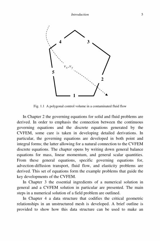
polygonal control volume of Fig. 1.1 placed in a steady incompressible
two-dimensional flow of a contaminated fluid. Assuming a unit depth
and a known fluid velocity field ),( yx vv=v , the fluid volume flow-rate
out across any one of the faces of this polygon is
dAqface
out ∫ ⋅= nv (1.1)
where n is the outward pointing normal on the face. Since the flow is
incompressible the net flow out of the volume is zero and given by

Basic Control Volume Finite Element Methods for Fluids and Solids
4
05
1
=⋅∑ ∫=face face
dAnv (1.2)
If there are contaminate sources and sinks in the domain of the fluid
flow, the contaminate concentration ),( yxC will vary throughout the
field. At any point in this field, the rate of contaminate transported per
unit area by the fluid motion (advection) is Cv and the rate of
contaminate transported by molecular diffusion (assuming isotropic
conditions and Fickian diffusion) is - C∇κ . In this way, the steady state
balance (net flow out) of the contaminate over the control volume shown
in Fig. 1.1 is given by
05
1
5
1
=⋅∇κ−⋅∑ ∑ ∫∫= =face face faceface
dACdAC nnv (1.3)
The conceptual heart of a Control Volume based numerical method is to
develop a means of approximating the integrals and derivatives in (1.3)
so as to reduce it to an algebraic equation; an equation written in terms of
the values of C at the discrete node points in the neighborhood of the
control volume.
To fully appreciate the concept used in the control volume approach it
is of high importance to note that equation (1.3) is an exact expression of
the underlying physics of the problem at hand. Although the governing
partial differential equation for this advection-diffusion problem is more
typically written in the point form
[ ] 0=∇⋅∇−⋅∇ CC κv , (1.4)
as will be emphasized in Chapter 2, the integral form in (1.3) is an
equally valid governing equation. Furthermore, as will be exploited in
Chapter 5, the integral form of the governing equation provides a clear
route toward obtaining the CVFEM discrete equations in terms of the
nodal values located at the centers of polygonal control volumes.
1.4 Main Topics Covered
The main topics covered in this monograph are as follows.
Introduction
5
Fig. 1.1 A polygonal control volume in a contaminated fluid flow
In Chapter 2 the governing equations for solid and fluid problems are
derived. In order to emphasis the connection between the continuous
governing equations and the discrete equations generated by the
CVFEM, some care is taken in developing detailed derivations. In
particular, the governing equations are developed in both point and
integral forms; the latter allowing for a natural connection to the CVFEM
discrete equations. The chapter opens by writing down general balance
equations for mass, linear momentum, and general scalar quantities.
From these general equations, specific governing equations for,
advection-diffusion transport, fluid flow, and elasticity problems are
derived. This set of equations form the example problems that guide the
key developments of the CVFEM.
In Chapter 3 the essential ingredients of a numerical solution in
general and a CVFEM solution in particular are presented. The main
steps in a numerical solution of a field problem are outlined.
In Chapter 4 a data structure that codifies the critical geometric
relationships in an unstructured mesh is developed. A brief outline is
provided to show how this data structure can be used to make an
1
2
3 4
5 yx v,v

Basic Control Volume Finite Element Methods for Fluids and Solids
6
automated link between the physics underlying the governing equation
and the discrete CVFEM equations.
In Chapter 5, working with a general advection-diffusion equation,
detailed derivations of the main components in a CVFEM are presented.
This is the essential knowledge kernel in this work.
In Chapter 6, in order to form a contrast, a brief presentation of the
development of a Control Volume Finite Difference Method for the
advection-diffusion equations is made.
In Chapter 7 the CVFEM of Chapter 5 is fully tested on a
comprehensive range of advection diffusion problems. The problems
chosen all have analytical solutions that provide meaningful testing of
the two-dimensional CVFEM operating on an unstructured grid. The
solutions span from steady state diffusion with constant diffusivity
through to transient advection-diffusion with variable properties.
In Chapter 8 the CVFEM solution for plane stress and plane strain
elasticity is developed. The application of this solution technology to the
problem of stress concentration around a hole in an infinite region
subjected to a uniform far-field stress is made. Comparisons between the
CVFEM and the known analytical solution are provided.
In Chapter 9 the CVFEM solution for the stream-function vorticity
form of the two-dimensional Navier Stokes equations for an
incompressible Newtonian fluid is developed. CVFEM solutions are
compared with results from a high-fidelity numerical benchmark
solution.
In Chapter 10 notes toward the developments of a three-dimensional
CVFEM are provided. In particular features of tetrahedral elements are
noted and the calculation for the flux across a control volume face is
presented.
In Appendix A a MATLAB code for generating a triangular mesh
with an appropriate CVFEM data structure is provided. Although this
mesh is based on a structured grid the resulting data structure can be used
with an unstructured CVFEM solution.
In Appendix B a MATLAB code for the CVFEM solution of a steady
sate advection diffusion equation is provided.

7
Chapter 2
Governing Equations
The governing equations for solid and fluid mechanics problems are
derived. Examples include advection-diffusion of a scalar, plane strain
and plane stress elasticity, and the stream function-vorticity formulation
of the Navier-Stokes flow equations.
2.1 The Euler Equations of Motion
The basic equations for describing motion of a deforming continuum
Ω —solid or liquid—are the Euler equations, expressing the
conservations of mass and linear momentum. These equations can be
derived in two ways, (i) performing a balance of mass or momentum on a
control volume fixed in space—referred to as the Eulerian approach or
(ii) tracking the rate of change of the mass or momentum in a specified
volume of the continuum as it moves through space—referred to as the
Lagrangian approach. For our purposes of developing Control Volume
Finite Element Method (CVFEM) solutions, the former Eulerian
description is the most appropriate.
2.1.1 Conservation of mass
In the Eulerian approach mass conservation is expressed as
∫ ∫ ⋅ρ−=ρ
V A
dAdVdt
dnv (2.1)

Basic Control Volume Finite Element Methods for Fluids and Solids
8
where V is a fixed volume in space—arbitrarily chosen from the
continuum Ω , A is the surface that encloses V, n is the outward
pointing unit normal at a point on this surface, x is the position
vector (from a fixed origin) to a point in V, )t,( xρ=ρ is the
density (mass/volume) at this point at time t, and )t,( xvv = is the
material velocity at point x at time t. Equation (2.1) states that the
rate of increase of the mass in V is given by the net rate of mass
flowing in across its surface A. On taking the time derivative under
the integral (volume V is fixed) and using the divergence theorem,
(2.1) can be written solely in terms of a volume integral,
∫ =ρ⋅∇+∂
ρ∂
V
dV)(t
0v (2.2)
2.1.2 Conservation of linear momentum
In the Eulerian approach, conservation of linear momentum is obtained
by applying Newton’s second law of motion to the fixed control volume
V
∫ ∫ ∫∫ ρ⋅−+ρ=ρ
V A AV
dA)(dAdVdVdt
dvnvtbv (2.3)
where )t,( xbb = is a body force and )t,,( nxtt = is the traction,
consisting of friction forces acting tangential to the surface A and
pressure forces acting normal to the surface A; as indicated in the
definition, the traction explicitly depends on the orientation of the
boundary over which it acts. The left hand side of (2.3) is the rate of
change of the linear momentum in V, which is balanced by the body
forces acting in V, the traction applied on the surface A of V, and the net
rate of linear momentum flowing into V across A. Through considering
the tractions on a vanishing tetrahedron and the angular momentum
balance it can be shown that the traction at a point x on area A can be
written in terms of a second order symmetric stress tensor σ and the unit
outward normal, i.e.,
nt σ= (2.4)

Governing Equations
9
or in index notation jiji nt σ= . In this way, on accounting for the fixed
nature of V, the momentum conservation in (2.3) can be written as
∫ ∫ ∫∫ ⋅−+=
V A AV
dA)(dAdVdVdt
dvnvnbv ρσρρ (2.5)
2.1.3 Conservation of scalar
In addition to conservation of mass and linear momentum we may also
need to express conservation of a scalar φ [quantity/mass], e.g., chemical
composition or heat. A relatively general form of this conservation over
the fixed volume V is
∫ ∫ ∫∫ ρφ⋅−⋅−ρ=ρφ
V A A
m
V
dA)(dAdVQdVdt
dnvnq (2.6)
where mQ is a mass source [quantity/mass-time] and q is a flux vector
[quantity/area-time]. In many cases the flux is a diffusion and
Ψ∇κ−=q (2.7)
where κ is a second order symmetric tensor and Ψ is a potential (e.g.,
temperature).
2.2 Specific Governing Equations
The integral forms of equations (2.1), (2.5) and (2.6) are most suitable
for the development of CVFEM solutions. To solve specific problem
types, however, it is necessary to define constitutive relationships for the
stress tensor σ in (2.5) and flux vector q in (2.6). The end objective in
such an exercise is to establish a set of governing equations where the
number of unknowns matches the number of equations. Below,
restricting attention to a Cartesian coordinate system where
)z,y,x()x,x,x( ≡321 and )v,v,v()v,v,v( zyx≡= 321v , examples of the
development of specific governing equations are provided.
Basic Control Volume Finite Element Methods for Fluids and Solids
10
2.2.1 Mass conservation in an incompressible flow
In an incompressible flow the rate of change of the density of a given
mass element following the fluid motion is zero, i.e., in terms of the
material derivative
0=∇⋅+∂
∂= ρ
ρρv
tDt
D (2.8)
Integrating this quantity over the fixed volume V and subtracting the
result from both sides of the mass conservation (2.2) results in the
following integral forms of mass conservation in an incompressible flow
0=⋅∇ρ∫V
dVv (2.9)
or through application of the divergence theorem
0=⋅∫A
dAnvρ (2.10)
Since the volume V in (2.9) is arbitrary and the density is positive and
non-zero 0>ρ , the divergence of the velocity must be identically zero
at every point in the domain,
Ω∈∀=⋅∇ xv ,0 (2.11)
i.e., a divergence-free velocity field is a point-form statement of mass
conservation in an incompressible fluid.
Note that, throughout this work, in addition to the rigorous statements
of incompressibility in (2.8)-(2.11) we will also use a slightly more
restrictive but operationally sound definition that in an incompressible
flow constant=ρ )t,( x .
2.2.2 Advection-diffusion of a scalar
If a conserved scalar φ, in an isotropic, incompressible (constant density)
continuum, has units of [conserved quantity/volume], and the flux vector
can be expressed in terms of the diffusive flux
φ∇κ−=q (2.12)

Governing Equations
11
where the scalar diffusivity κ has units [area/time], the conservation
(2.6) can be written as
∫∫∫∫ φ⋅−⋅φ∇κ+=φ
AAVV
dA)(dAndVQdVdt
dnv (2.13)
where Q [quanity/volume-time] is a volume source term. Taking the
time derivative inside the volume integral (recall V is fixed in space) and
using the divergence theorem we arrive at
0∫ =−φ∇κ⋅∇−φ⋅∇+∂
φ∂
V
QdV)()(t
v
Or since the volume V is chosen arbitrarily the argument has to be
identically zero at every point in the domain, i.e.,
0=−φ∇κ⋅∇−φ⋅∇+∂
φ∂Q)()(
tv (2.14)
which should be immediately recognized as the point form of the well
known transient advection diffusion equation. The derivation of (2.14) is
made to emphasize the connection between the integral forms of the
conservation equations, like those given in (2.6) and (2.13), and the more
familiar and pervasive point forms like (2.14). In choosing between these
two alternative balance statements, however, it will be repeatedly
stressed throughout this work that the integral forms are the most suitable
for developing numerical solutions based on Control Volume Finite
Element technologies.
2.2.3 Stress and strain in an elastic solid
In determining the mechanical state (stresses and strains) in a body
subjected to a loading, if we restrict attention to cases where translational
and rotational rigid body motions do not occur and the body deforms but
does not flow, we need only consider the linear momentum balance
∫ ∫ =σ+ρ
V A
dAdV 0nb (2.15)

Basic Control Volume Finite Element Methods for Fluids and Solids
12
obtained by setting the velocity v = 0 in (2.5). If we interpret the stress as
the measure of change from an initial state of equilibrium and assume the
body force remains unchanged during this evolution, the body force term
can be dropped to arrive at
∫ =σ
A
dA 0n (2.16)
Through the divergence theorem this equation can be written as a single
volume integral, in index notation
0=∂
σ∂
∫V j
ijdV
x (2.17)
or, since V is arbitrarily chosen, the point form
0=∂
σ∂
j
ij
x (2.18)
This last equation, the well known form of the equilibrium equation
written in terms of change in stress, and is an often used starting point
for the development of numerical solutions of solid mechanics problems.
In this work, however, it is more convenient and direct to retain the
alternative integral form in (2.16) or (2.17).
In further developing the statement (2.17) it is first noted that, if the
loading of an isotropic, linear elastic body results in small deformations
(compared to the dimension of the body as a whole) the stress can be
related to the strain through the “generalized” Hooke’s law;
)(E
)())((
Eijijijkkkkij00
1211ε−ε
ν++δ
ε−ε
ν−ν+
ν=σ (2.19)
where, due to the small deformation assumption, the relationship
between strains ijε and displacements ui is
∂
∂+
∂
∂=ε
j
i
i
jij
x
u
x
u
2
1 (2.20)
and
Governing Equations
13
∂
∂+
∂
∂+
∂
∂=
∂
∂=ε
z
u
y
u
x
u
x
u zyx
k
kkk (2.21)
In the above E is the Young’s modulus [force/area], ν is Poisson’s ratio,
and ijδ =1 if i = j, ijδ =0 if ji ≠ is the Kronecker delta. The tensor 0ijε is
an initial strain—a strain independent of the stress; e.g., an isotropic
thermal expansion,
ijij Tδ∆α=ε0 (2.22)
where α is the thermal expansion coefficient and T∆ is the temperature
change from a reference state.
Substitution of (2.19) - (2.22) into (2.16) results in an integral
equation in terms of the displacements. In component form, for a
Cartesian coordinate system
01212
11
211
=
∂
∂+
∂
∂
ν++
∂
∂+
∂
∂
ν++
∆α
ν
ν+−
∂
∂+
∂
∂+
∂
∂
ν
ν−
ν−ν+
ν∫
dAnz
u
x
u
)(
En
y
u
x
u
)(
E
nTz
u
y
u
x
u
))((
E
zxz
yxy
A
xzyx
012
11
211
12
=
∂
∂+
∂
∂
ν++
∆α
ν
ν+−
∂
∂+
∂
∂
ν
ν−+
∂
∂
ν−ν+
ν+
∂
∂+
∂
∂
ν+∫
dAnz
u
y
u
)(
E
nTz
u
y
u
x
u
))((
E
ny
u
x
u
)(
E
z
yz
yzyx
A
xxy
(2.23)
011
211
1212
=
∆α
ν
ν+−
∂
∂
ν
ν−+
∂
∂+
∂
∂
ν−ν+
ν+
∂
∂+
∂
∂
ν++
∂
∂+
∂
∂
ν+∫
dAnTz
u
y
u
x
u
))((
E
dAnz
u
y
u
)(
En
z
u
x
u
)(
E
zzyx
y
yz
A
xxz
Basic Control Volume Finite Element Methods for Fluids and Solids
14
Equation (2.23) is a general statement for the displacements in a three-
dimensional body. Two important, two-dimensional cases of this
equation are considered in this work.
2.2.4 Plane stress
If the domain of the problem is much thinner in a given direction, z-say,
the stresses in that direction can be neglected, i.e.,
0=σ=σ=σ zzyzxz (2.24)
This condition, referred to as the plane stress condition, essentially
reduces solution of (2.23) to a two-dimensional problem in the x-y plane.
On using the stress-strain relationship in (2.19) and the strain definition
in (2.20) and (2.21) the conditions in (2.24) lead to the following
relationships in displacements
0=∂
∂+
∂
∂
z
u
x
u xz , (2.25)
0=∂
∂+
∂
∂
z
u
y
u yz , (2.26)
and
Ty
u
x
u
z
u yxz ∆αν−
ν++
∂
∂
ν−
ν−
∂
∂
ν−
ν−=
∂
∂
1
1
11 (2.27)
On substitution in (2.23) and recognizing, in the two-dimensional case,
that the area integrals are over a closed curve, these relationships lead to
a system in terms of displacements in the x-y plane alone, i.e.,
012
11 2
=
∂
∂+
∂
∂
ν++
∆αν+−
∂
∂ν+
∂
∂
ν−∫
dSny
u
x
u
)(
E
nT)(y
u
x
u
)(
E
yxy
x
yx
S
(2.28)

Governing Equations
15
011
12
2=
∆αν+−
∂
∂+
∂
∂ν
ν−+
∂
∂+
∂
∂
ν+∫
dSnT)(y
u
x
u
)(
E
ny
u
x
u
)(
E
yyx
S
xxy
(2.29)
Or, following Fryer et al (1991), the more appropriate form for a control
volume solution
∫
∫
=∂
∂
ν−+
∂
∂
ν+
=∂
∂
ν++
∂
∂
ν−
S
yy
y
x
y
xyx
S
xx
SdSny
u
)(
En
x
u
)(
E
SdSny
u
)(
En
x
u
)(
E
2
2
112
121 (2.30)
Where
∫
∫
=
∆αν+−
∂
∂ν
ν−+
∂
∂
ν+−=
=∂
∂
ν++
∆αν+−
∂
∂ν
ν−−=
S
yx
xx
y
y
y
x
y
S
x
dSnT)(x
u
)(
En
y
u
)(
ES
dSnx
u
)(
EnT)(
y
u
)(
ES
01112
012
11
2
2
The in-plane stresses resulting from the displacement fields in (2.28)
and (2.29) are
∆αν+−
∂
∂ν+
∂
∂
ν−=σ T)(
y
u
x
u
)(
E yxxx 1
1 2
∂
∂+
∂
∂
ν+=σ
y
u
x
u
)(
E xy
xy12
(2.31)
∆αν+−
∂
∂+
∂
∂ν
ν−=σ T)(
y
u
x
u
)(
E yxyy 1
1 2

Basic Control Volume Finite Element Methods for Fluids and Solids
16
2.2.5 Plane strain
In contrast to the plane stress case, if the domain has a constant cross-
section, much thicker in the z-direction, the strains (but not the stresses)
can be neglected in that direction, i.e.,
0=ε=ε=ε zzyzxz (2.32)
This condition, referred to as the plane strain condition, can also reduce
solution (2.23) to a two-dimensional problem in the x-y plane. Through
the definition of strain in (2.20) and (2.21), the conditions (2.32) allows
for (2.23) to be written in two closed equations for the displacements in
the x-y plane, i.e.,
012
11
211
=
∂
∂+
∂
∂
ν++
∆α
ν
ν+−
∂
∂+
∂
∂
ν
ν−
ν−ν+
ν∫
dSny
u
x
u
)(
E
nTy
u
x
u
))((
E
yxy
S
x
yx
(2.33a)
011
211
12
=
∆α
ν
ν+−
∂
∂
ν
ν−+
∂
∂
ν−ν+
ν
+
∂
∂+
∂
∂
ν+∫
dSnTy
u
x
u
))((
E
ny
u
x
u
)(
E
y
yx
S
xxy
(2.33b)
which can be rearranged
yy
y
S
x
y
xyx
S
xx
SdSny
u
))((
)(En
x
u
)(
E
SdSny
u
)(
En
x
u
))((
)(E
=∂
∂
ν−ν+
ν−+
∂
∂
ν+
=∂
∂
ν++
∂
∂
ν−ν+
ν−
∫
∫
211
1
12
12211
1
(2.34)
where, in this case,

Governing Equations
17
01
211
12
012
1
211
=
∆α
ν
ν+−
∂
∂
ν−ν+
ν
+∂
∂
ν+−=
=∂
∂
ν++
∆α
ν
ν+−
∂
∂
ν−ν+
ν−=
∫
∫
dSnTx
u
))((
E
ny
u
)(
ES
dSnx
u
)(
E
nTy
u
))((
ES
yx
S
xx
y
y
y
S
x
y
x
The in-plane stresses resulting from the displacement fields in (2.33)
are
∆α
ν
ν+−
∂
∂+
∂
∂
ν
ν−
ν−ν+
ν=σ T
y
u
x
u
))((
E yxxx
11
211
∂
∂+
∂
∂
ν+=σ
y
u
x
u
)(
E xy
xy12
(2.35)
∆α
ν
ν+−
∂
∂
ν
ν−+
∂
∂
ν−ν+
ν=σ T
y
u
x
u
))((
E yxyy
11
211
2.2.6 Relationship between plane stress and plane strain
In developing codes to solve the plane stress and plane strain problems
derived above it is not necessary to develop two separate codes. Rather,
it is much more convenient to switch between plane stress and plane
strain by simply defining “compound” material constants. For example,
it is relatively easy to show (Barber (2003)) that the replacement of the
Young’s modulus, Possion’s ratio, and thermal coefficient of expansion
in the plane stress equations (2.29) by the compound constants
αν+=αν−
ν=ν
ν−= )(,,
EE
*** 111 2
(2.36)

Basic Control Volume Finite Element Methods for Fluids and Solids
18
results in the plane strain formulation in (2.33). Hence, if a plane stress
code is available a given plane strain problem can be readily computed
on using the compound material constants in (2.36) in place of the given
constants.
2.2.7 The Navier-Stokes equations
In the previous treatment specific two-dimensional equations for the
displacements in an elastic loaded body have been derived from a
general three-dimensional form. The intention now is to repeat this
exercise to arrive at a description of the flow field in a two-dimensional
domain from a general three dimensional form.
To fully describe the velocity field in a flow we need to develop mass
and momentum conservation equations. The basic case to study is the
flow of an incompressible Newtonian flow (shear stress proportional to
strain rate). The appropriate integral and point forms for the mass
conservation are given in (2.8)-(2.11), hence the requirement here is to
develop a momentum conservation equation in terms of the unknown
velocity field, v.
In general, the stress tensor σ in a flowing fluid can be written as the
sum of an isotropic part involving the pressure and a non-isotropic or
deviatoric part involving the tangential stresses (Batchelor (1970)). In
index notation
)(p ijkkijijij δε−εµ+δ−=σ ɺɺ312 (2.37)
where p is the pressure, and ijεɺ is the strain-rate tensor—note the over-
script dot used to distinguish this from the strain tensor ijε introduced in
the linear elasticity equations— and µ is the dynamic viscosity. In a
Newtonian fluid—the strain rate is related to the velocities
∂
∂+
∂
∂=ε
i
j
j
iij
x
v
x
v
2
1ɺ (2.38)
and, if the flow is incompressible (see (2.11)) the term
Governing Equations
19
0=⋅∇=∂
∂+
∂
∂+
∂
∂≡
∂
∂=ε v
z
v
y
v
x
v
x
v wyx
k
kkkɺ (2.39)
In this way, on substituting for σ , the momentum balance (2.5) for a
Newtonian incompressible fluid can be written as
∫ ∫∫∫
∫∫
ρ−∂
∂µ+
∂
∂µ+−
ρ=ρ
A A
ijj
A
ji
j
A
jj
ii
V
i
V
i
dAvnvdAnx
vdAn
x
vdApn
dVbdVvdt
d
(2.40)
On using the divergence theorem, and, moving the time derivative under
the integral sign (remember the volume V is fixed) (2.40) can be written
solely in terms of an integration over the control volume
( )∫ ∫∫∫
∫∫
ρ∂
∂−
∂
∂µ
∂
∂+
∂
∂µ
∂
∂+
∂
∂−
ρ=∂
ρ∂
V V
jijV i
j
jV j
i
ji
V
i
V
i
dVvvx
dVx
v
xdV
x
v
xdV
x
p
dVbdVt
)v(
(2.41)
If the viscosity is constant, this equation can be further simplified by
switching the order of differentiation in the 4th term on the right hand
side and noting that—due to the condition of incompressibility—
0=⋅∇≡∂∂ vjj x/v to arrive at
( )∫ ∫∫
∫∫
ρ∂
∂−
∂
∂
∂
∂µ+
∂
∂−
ρ=∂
ρ∂
V V
jijV j
i
ji
V
i
V
i
dVvvx
dVx
v
xdV
x
p
dVbdVt
)v(
(2.42)
Since the volume V is arbitrary this can be written as
( )
∂
∂
∂
∂µ+
∂
∂−ρ=ρ
∂
∂+
∂
ρ∂
j
i
jiiji
j
i
x
v
xx
pbvv
xt
)v( (2.43)

Basic Control Volume Finite Element Methods for Fluids and Solids
20
which can be identified as the conserved point form of the Navier-Stokes
equation for an incompressible constant viscosity flow. The non-
conserved form, arrived at by expanding the left and side and using the
incompressibility condition
0=ρ∇⋅+∂
ρ∂v
t,
is
∂
∂
∂
∂µ+
∂
∂−ρ=
∂
∂ρ+
∂
∂ρ
j
i
jii
j
ij
i
x
v
xx
pb
x
vv
t
v (2.44)
2.2.8 The stream-function—vorticity formulation
In this work we will only concern ourselves with solving steady,
incompressible, constant property ( ), constant=µρ flow problems in
two-dimensional (x-y) domains. For this case, in the absence of body
forces, the momentum balance equation (2.42) can be written as
( ) 01 2 =∇ν−
∂
∂
ρ+⋅∇∫ dAv
x
pv
A
xxv (2.45a)
( ) 01 2 =∇ν−
∂
∂
ρ+⋅∇∫ dAv
y
pv
A
yyv (2.45b)
where ρµ=ν / is the kinematic viscosity. Note in this two-dimensional
case the control volume V is now a control area A and the nabla symbol
is defined as )y/,x/( ∂∂∂∂≡∇ . In seeking a solution of (2.45) it is
convenient to eliminate the pressure p. This can be achieved by taking
the partial derivative of (2.45a) with respect to y and subtracting the
result from the partial derivate of (2.45b) with respect to x. After some
manipulation and rearrangement this arrives at the single momentum
conservation equation with the advection-diffusion form
02 =ω∇ν−⋅∇∫
A
dA)ω( v (2.46)
where
Governing Equations
21
y
v
x
vxy
∂
∂−
∂
∂=ω (2.47)
is the vorticity. Progress is made by introducing the stream function
defined by
x
v,y
v yx∂
Ψ∂−=
∂
Ψ∂= (2.48)
Note this definition automatically satisfies the incompressibility
conditions (2.8)-(2.11) and allows the vorticity to be related to the stream
function via (2.47)
ω−=Ψ∇2 (2.49)
Appropriate integral forms suitable for a CVFEM solution can be
obtained by using the divergence theorem to transform the area integrals
into surface integrals. In particular (2.46) can be written as
0=⋅ω∇ν−⋅ω∫ dS
S
nnv (2.50)
and (2.49) can be written as
∫ ∫ ⋅ψ∇=ω−
A S
dSdA n (2.51)
In a CVFEM application, an iterative solution, is constructed; for a given
velocity field, a discrete form of (2.50) is solved for ω , followed by a
solution of a discrete form of (2.51) for Ψ , and a velocity update by
(2.48).

22
Chapter 3
The Essential Ingredients in a Numerical
Solution
The essential ingredients in numerical solution for the field problems of
Chapter 2 are outlined and discussed.
3.1 The Basic Idea
The field problems governed by the equations of Chapter 2 operate over
a spatial domain with conditions, in terms of the dependent variables and
their derivatives, prescribed on the boundary. A closed analytical
solution of the governing equations provides a continuous function, such
that for any given point in the problem domain values of the dependent
variables can be calculated exactly. Closed form solutions, however, can
only be derived for a limited number of special cases and, in general, a
numerical solution needs to be constructed. The essential feature in a
numerical solution is to obtain a discrete solution where values of the
dependent variables are only obtained at a set of distinct points
distributed throughout the domain—the node points; solution values at
other points can be obtained by interpolation of the local node values.
The nodal values of the dependent variables are obtained from the
solution of an algebraic set of equations that relate the dependent
variables at a given node point to the values at neighboring nodes.
Appropriate algebraic equations—referred to as discrete equations—are
obtained by one of two ways. The first approach uses suitable
mathematical treatments of the governing equations in Chapter 2, e.g.,
finite difference approximations of terms in the equation, Smith (1985)
or the method of weighted residuals, Zienkiewicz and Taylor (1989).

The Essential Ingredients in a Numerical Solution
23
The second approach—and the one adopted in this work—is to arrive at
discrete equations based on consideration of the same physical principals
used to derive the continuous governing equations in Chapter 2. This
approach is referred to as the Control Volume Method (CVM), Patankar
(1980). The objective of this chapter is to provide a description of the
key ingredients in developing a Control Volume solution.
3.2 The Discretization: Grid, Mesh, and Cloud
The initial step of arriving at the discrete equations is to place the node
points into the domain. Broadly speaking there are three ways in which
this can be achieved.
3.2.1 Grid
A basic approach assigns the location of nodes using a structured grid
where, in a two-dimensional domain, the location of a node is uniquely
specified by a row and a column index, see Fig. 3.1a. Although such a
structured approach can lead to very convenient and efficient discrete
equations it lacks flexibility in accommodating complex geometries or
allowing for the local concentration of nodes in solution regions of
particular interest.
3.2.2 Mesh
Geometric flexibility, usually at the expense of solution efficiency, can
be added by using an unstructured mesh. Fig. 3.1b shows an unstructured
mesh of triangular elements. In two dimensional domains triangular
meshes are good choices because they can tessellate any planar surface.
Note however, other choices of elements can be used in place of or in
addition to triangular elements. The mesh can be used to determine the
placement of the nodes. A common choice is to place the nodes at the
vertices of the elements. In the case of triangles, this will allow for the
approximation of a dependent variable, over the element, by linear

Basic Control Volume Finite Element Methods for Fluids and Solids
24
Fig. 3.1 Different forms of discretization
interpolation between the vertex nodes. Higher order approximations can
be arrived at by using more nodes (e.g., placing nodes at mid points)
and/or alternative elements (e.g., quadrilaterals).
In considering an unstructured mesh it is important to recognize that
the following:
1. The quality of the numerical solution obtained is critically dependent
on the mesh. For example, a key quality requirement for a mesh of
i
i
row1
row2
row3
row4 col1 col2 col3 col4
a. Grid
b. Mesh
c. Cloud
The Essential Ingredients in a Numerical Solution
25
triangular elements is to avoid highly acute angles. The generation of
appropriate meshes for a given domain is a complex topic worthy of
a monograph in its own right. Fortunately, for two-dimensional
problems in particular, there is a significant range of commercial and
free software that can be used to generate quality meshes, e.g., the
Delaunay triangularization routines in MATLAB used to create Fig.
3.1b.
2. The term unstructured is used to indicate a lack of a global structure
that relates the position of all the nodes in the domain. In practice,
however, a local structure—the region of support—listing the nodes
connected to a given node i, is required. Establishing, storing and
using this local data structure is one of the critical ingredients in
using an unstructured mesh (see Chapter 4).
3.2.3 Cloud
The most flexible discretization is to simply populate the domain with
node points that have no formal background grid or mesh connecting the
nodes. Solution approaches based on this mesh-less form of
discretization create local and structures, usually based on the “cloud” of
neighboring nodes that fall with in a given length scale of a given node i,
see Fig. 3.1c. A discussion of the features of meshless solutions can be
found in Pepper (2006).
3.2.4 Discretizations for the Control Volume Finite Element Method
CVFEM solutions are based on a mesh of elements. The main
discretization used in this work will be meshes of two-dimensional
triangular elements (Fig. 3.1b). In the following discussion the
components of this form of mesh and its role in a CVFEM solution are
examined in detail.
3.3 The Element and the Interpolation Shape Functions
As noted previously, the building block of the discretization is the
triangular element, Fig. 3.2. For linear triangular elements the node

Basic Control Volume Finite Element Methods for Fluids and Solids
26
points are placed at the vertices. In Fig. 3.2 the nodes, moving in a
counter-clockwise direction, are labeled 1, 2 and 3. Values of the
dependent variable φ are calculated and stored at these node points. In
this way, values at an arbitrary point )y,x( within the element can be
approximated with linear interpolation
cbyax ++≈φ (3.1)
where the constant coefficients a, b and c satisfy the nodal relationships
321 ,,i,cbyax iii =++=φ (3.2)
Equation (3.1) can be more conveniently written in terms of the shape
function ,N,N 21 and 3N , where
=i node opposite sideon points allat 0,
i nodeat 1,)y,x(N i (3.3)
element in thepoint every at 13
1
,)y,x(N
i
i =∑=
(3.4)
such that, over the element, the continuous unknown field can be
expressed as the linear combination of the values at nodes 321 ,,i =
∑=
φ≈φ3
1i
ii )y,x(N)y,x( (3.5)
With linear triangular elements a straightforward geometric
derivation for the shape functions can be obtained. With reference to
Fig. 3.2, observe that the area of the element is given by
)]xx(y)yy(x)yxyx[(
yx
yx
yx
A
2312312332
33
22
11123
2
1
1
1
1
2
1
−+−−−=
=
(3.6)
and the area of the sub-elements with vertices at points ),,p( 32 ,
),,p( 13 , and ),,p( 21 , where p is an arbitrary and variable point in the
element, are given by

The Essential Ingredients in a Numerical Solution
27
)]xx(y)yy(x)yxyx[(A ppp
2323233223
2
1−+−−−= (3.7a)
)]xx(y)yy(x)yxyx[(A ppp
3131311331
2
1−+−−−= (3.7b)
)]xx(y)yy(x)yxyx[(A ppp
1212122112
2
1−+−−−= (3.7c)
With these definitions it follows that the shape functions are given by
123123
123312
123231 A/AN,A/AN,A/AN
ppp === (3.8)
Note that, when point p coincides with node i (=1, 2 or 3) the shape
function 1=iN , and when point p is anywhere on the element side
opposite node i, the associated sub-element area is zero, and through
(3.8), the shape function 0=iN . Hence the shape functions defined by
(3.8) satisfy the required condition in (3.3). Further, note that at any
point p , the sum of the areas
123123123AAAA
ppp =++
such that the shape functions at )y,x( pp will sum to unity. Hence the
shape functions defined by (3.8) also satisfies the condition (3.4).
For future reference it is worthwhile to note that the derivatives of the
shape functions in (3.8) over the element are the following constants
123
1233123
2133
123
3122123
1322
123
2311123
3211
22
22
22
A
)xx(
y
NN,
A
)yy(
x
NN
A
)xx(
y
NN,
A
)yy(
x
NN
A
)xx(
y
NN,
A
)yy(
x
NN
yx
yx
yx
−=
∂
∂=
−=
∂
∂=
−=
∂
∂=
−=
∂
∂=
−=
∂
∂=
−=
∂
∂=
(3.9)

Basic Control Volume Finite Element Methods for Fluids and Solids
28
Fig. 3.2 An element indicating the areas used in shape function definitions
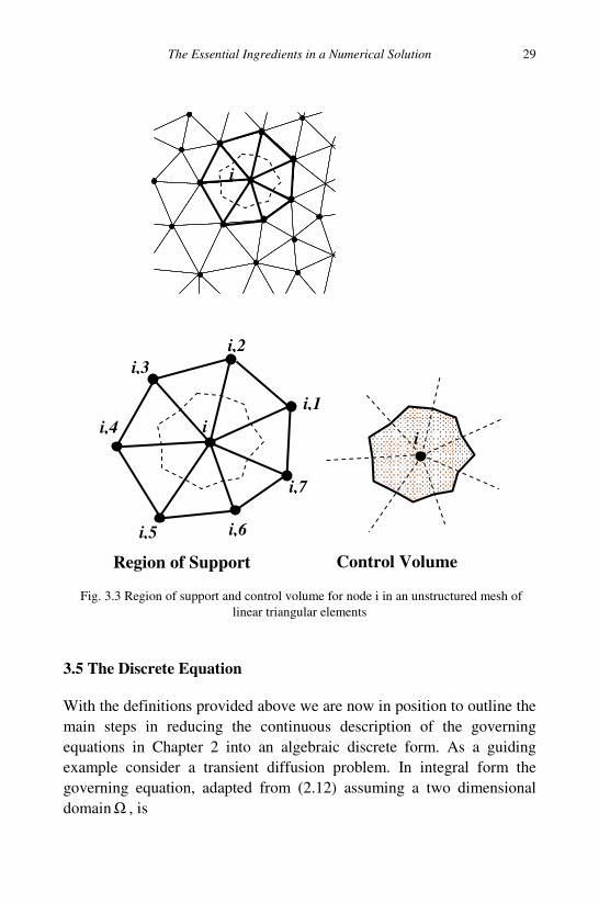
3.4 Region of Support and Control Volume
The local structure on the mesh in Fig. 3.1b is defined in terms of the
region of support—the list of nodes that share a common element with a
given node i, in Fig. 3.3. In this region of support, as illustrated in Fig.
3.3, a control volume is created by joining the center of each element in
the support to the mid points of the element sides that pass through
node i . This creates a closed polygonal control volume with 2m sides
(faces); where m is the number of elements in the support. Each element
contributes 1/3 of its area to the control volume area and the volumes
from all the nodes tessellate the domain without over lap. As noted
below, in arriving at the discrete numerical equation, the control volume
is related to the domain of integration in the integral forms of the
governing equations in Chapter 2.
1
2
3
1
2
3
1
2
3
1
2
3
p p p
123A
23pA
31pA
12pA
The Essential Ingredients in a Numerical Solution
29
Fig. 3.3 Region of support and control volume for node i in an unstructured mesh of
linear triangular elements
3.5 The Discrete Equation
With the definitions provided above we are now in position to outline the
main steps in reducing the continuous description of the governing
equations in Chapter 2 into an algebraic discrete form. As a guiding
example consider a transient diffusion problem. In integral form the
governing equation, adapted from (2.12) assuming a two dimensional
domain Ω , is
i
i
i,1
i,2
i,3
i,4
i,5 i,6
i,7
Region of Support Control Volume
i

Basic Control Volume Finite Element Methods for Fluids and Solids
30
Ω∈⋅φ∇κ=φ ∫∫SA
,dSndAdt
dx (3.10)
As indicated in Fig. 3.4a, the domain in the integral (3.10) can be any
arbitrary closed area in Ω , including areas that share common surfaces
with the boundary Γ of Ω .
The steps in converting (3.10) into a set of discrete algebraic
equations in terms of the nodes distributed thought out Ω are as follows.
1. The domain is covered by a mesh of triangular elements, Fig. 3.4b.
2. The regions of support and control volumes attached to each node i are
identified; this requires that an appropriate data structure is used, see
Chapter 4.
3. The domains of the integrals in (3.10) are associated with the regions
of support, Fig. 3.4b.
4. Using numerical integration (usually one-point rules) and the shape
function approximations (3.5) of φ in each element of the ith support,
equation (3.10) is expanded in terms of the nodal values of φ in the
support.
5. On gathering terms, the resulting equation for node i can be written in
the general discrete form
∑ +φ=φnb
inbnbii baa (3.11)
where ai and anb are coefficients for the unknown nodal values of φ , and
the additional coefficient bi accounts for contributions from sources,
transients and boundaries. Equation (3.11) provides an algebraic
relationship between the value of φ at node i and the neighboring (nb)
nodes in its support.
The central task of this text is to provide a detailed “recipe” for the
determination of the coefficients in (3.11) for a given governing field
equation and domain mesh. The main approach used is based on the
control volume concept laid out above. Note, however, that any
numerical method based on a domain discretization (grid, mesh, or
cloud) can, regardless of the mathematical sophistication employed, be
written in the form (3.11).

The Essential Ingredients in a Numerical Solution
31
Fig. 3.4 Association between area domain in integral forms of the governing equation
and the components of the discretization mesh
domain boundary
Ω
Γ
A
S
a. b.
32
Chapter 4
Control Volume Finite Element Data Structure
An unstructured mesh data structure for control volume finite elements is
presented.
4.1 The Task
In Chapter 3 the essential components in a domain discretization, i.e.,
nodes, mesh, elements, region of support, and control volume, were
defined. This chapter outlines how these components are used to reduce a
continuous governing field equation into a set of discrete equations in
terms of unknown nodal values. In order to automate this process
through the use of a computer code it is necessary to provide a data
structure that can identify and store the mesh components (elements,
support, control volume) associated with a given node point in the
solution domain. Providing a suitable data structure for a Control
Volume Finite Element Method (CVFEM) code is the current objective.
Emphasis is placed on the term suitable to indicate that there is not a
unique form for the data structure. In this respect, it is noted that the data
structure presented here is not designed for efficiency or compactness but
for clarity of presentation.
4.2 The Mesh
The starting point for the data structure presented here is to cover the
solution domain with a mesh of linear triangles. As noted in Chapter 3,
there are a number of commercial and open source codes that will
generate high quality unstructured meshes that will be compatible with
Control Volume Finite Element Data Structure
33
the data structure used in this work. The basic requirements are that these
mesh generators provide
1. a contiguous and unique numbering (labeling) of the nodes
)n,...,,i( 21= , where n is the number of nodes in the domain
discretization,
2. a vector of the nodal x and y positions, i.e., ix and iy ,
3. a contiguous unique numbering of the triangles in the discretization.
4. A listing of the node numbers (labels) of the vertices of the triangles
(preferably in counter-clockwise order), and
5. a listing of the nodes that lie on the boundary of the domain.
It is recognized that it may not be possible or easy for a reader to find
an unstructured mesh generator. To compensate for this a meshing code,
based on a structured grid, is provided in Appendix A. This code,
discussed in more detail in Appendix A, provides a “ready-to-use” mesh
conforming to the required data structure.
4.3 The Data Structure
There are two central components in the data structure, the region of
support for a node i in the domain discretization and the domain
boundaries.
4.3.1 The region of support
Figure 4.1 shows a domain mesh which possesses the five informational
attributes noted in the previous section. For each node i in the mesh the
region of support is identified by counting and listing all the neighboring
nodes k that share a common element side with node i . The number of
neighboring nodes in the region of support is stored in the variable sin
where the index n...,,i 21= . The nodes in the region of support of node i
are stored in the two-dimensional array j,iS , where the index n...,,i 21=
and the index 121 += si
si n,n,...,j . For a specific example refer to Fig. 4.1
Basic Control Volume Finite Element Methods for Fluids and Solids
34
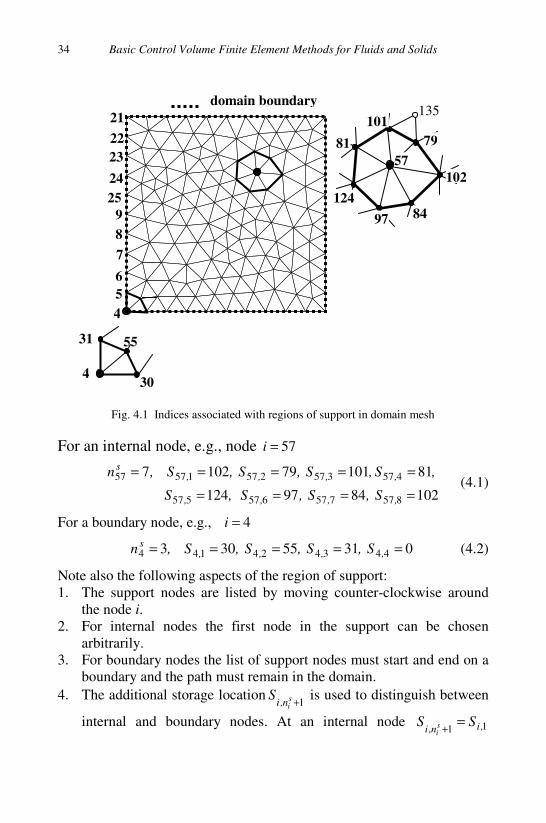
Fig. 4.1 Indices associated with regions of support in domain mesh
For an internal node, e.g., node 57=i
1028497124
81101791027
857757657557
45735725715757
====
=====
,,,,
,,,,s
S,S,S,S
,S,S,S,S,n (4.1)
For a boundary node, e.g., 4=i
03155303 443424144 ===== ,,,,s
S,S,S,S,n (4.2)
Note also the following aspects of the region of support:
1. The support nodes are listed by moving counter-clockwise around
the node i.
2. For internal nodes the first node in the support can be chosen
arbitrarily.
3. For boundary nodes the list of support nodes must start and end on a
boundary and the path must remain in the domain.
4. The additional storage location1+s
in,iS is used to distinguish between
internal and boundary nodes. At an internal node 11 ,in,iSS s
i
=+
57
102
79
101
81
124
97 84
135 domain boundary
55
4
31
30
21
4
22
24
23
8
5
25
9
7
6

Control Volume Finite Element Data Structure
35
indicating complete enclosure of node i. At a boundary node
01
=+e
in,iS .
4.3.2 The boundary
In addition to the region of support it is also important to store
information on the domain boundaries. First the boundary is segmented
into segn contiguous sections, identified by a common boundary
condition, e.g., an imposed value or an imposed flux. Then, for a given
boundary segment the global node numbers on the boundary are stored in
the two-dimensional array j,kB where the index k is over the boundary
segments, i.e., segn,....,k 21= and the index j is over the nodes on the
boundary, i.e., k,Bn,....,j 21= ( =k.Bn the number of nodes on boundary
segment).
Assume the 4 obvious boundary segments in the domain in Fig 4.1
and number these segments counter clockwise starting from the lower
horizontal boundary. In this case the data structure for the left hand
vertical boundary is
456
78925
24232221
11
11410494
84746454
44342414
4
===
====
====
=
,,,
,,,,
,,,,
b
B,B,B
,B,B,B,B
,B,B,B,B
,n
(4.3)
Again note the counter clockwise counting of the boundary segments and
the nodes on the segment.
4.4 The Discrete Equation
The key objective of a CVFEM is to reduce the integral from of a
governing field equation, e.g.,
Ω∈⋅φ∇κ=φ ∫∫SA
,dSndAdt
dx (4.4)

Basic Control Volume Finite Element Methods for Fluids and Solids
36
to a set of discrete algebraic equations in the unknown nodal values of φ .
With the data structure given above the form of this equation, derived
from (3.11) is
∑=
+φ=φi
j,i
N
j
iSj,iii baa
1
(4.5)
where ia is the coefficient associated with the unknown at node i , j,ia is
the coefficient associated with the thj node in the th
i support, and ib
accounts for contributions from sources, transients and boundaries.
Figure 4.2 summarizes how the data structure and geometric components
of the numerical mesh are used to automate the process of extracting
(4.4) from (4.3). The steps in this automation are as follows.
1. For a given element in the support of i , a local node numbering [1,
2, 3] is employed. In the jth element of support i this local numbering
is related to the global nodes through the identity
[1, 2, 3] = [i, Si,j, Si,j+1] (4.6)
Note that local node 1 is always associated with node i and the
remaining two nodes in the element are numbers in a counter
clockwise fashion.
2. For each node j in the support of node i , the element in (4.6) is
identified. Since the global node numbers of the vertices are known
through (4.6), the local coordinates of the vertices in the element can
be accessed by pointing to
1
1
321
321
+
+
===
===
j,ij,i
j,ij,i
SSi
SS,i
yy,yy,yy
xx,xxxx (4.7)
3. Equation (4.6) allows for the calculation of all the geometric features
of the element. In particular, (i) its area jA , (ii) the contribution of
this area ( jA
31 ) to the control volume area iA ,(iii) its linear shape
functions 321 N,N,N and their derivatives, (iv) the unit normal on
the faces of the control volume that reside in the element, and (v) the
lengths of these faces. As detailed in Chapter 5, this is sufficient
information to carry out a numerical integration of the surface
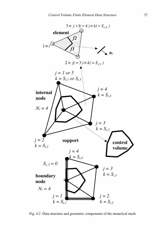
Control Volume Finite Element Data Structure
37
Fig. 4.2 Data structure and geometric components of the numerical mesh
i
control
volume
support
j = 4
k = Si,4
j = 1 or 5
k = Si,1 or Si,5
j = 2
k = Si,2
j = 3
k = Si,3
i
internal
node
j = 1
k = Si,1
Ni = 4
boundary
node
j = 2
k = Si,2
j = 3
k = Si,3
Si,,5 = 0
j = 4
k = Si,4
Ni = 4
element
f1
)S(k)(j ,i 332 =≡=≡
i≡1
)S(k)(j ,i 4413 =≡=+≡
nf
f2

Basic Control Volume Finite Element Methods for Fluids and Solids
38
integral on the right hand side of (4.4). A step that essentially
approximates the fluxes crossing the two control volume faces,
1f and 2f in the element in question in terms of the nodal values
1+φφφ
j,ij,i SSi ,, .
4. When the loop around the support of node is complete, i.e., the
above calculations have been carried out for each element in the
domain, the right hand side of (4.4) is fully determined. That is, the
net flux crossing the faces of the control volume around node i are
fully determined in terms of the nodal values at node i and its
support. At the same time, summing the contributions ( jA
31 ) from
each element the area of the control volume is known. This value can
be immediately used in a mid-point integration of the left hand side
of (4.4) that will add additional dependencies on the nodal values to
(4.5).
5. Appropriate gathering of the terms from steps 3 and 4 will allow for
the identification of the coefficients in the general discrete equation
(4.4). The process can be repeated for each node in the domain to
arrive at closed systems of equations in terms of all the nodal values
of φ .
4.5 Summary
This chapter has proposed a data structure for the use with a CVFEM
code and discussed how this data structure can be used to automatically
generate the CVFEM discrete equations in (4.5). The five steps identified
in the previous section, however, only provide a sketch of how the
proposed data structure is used to obtain the coefficients in (4.5). Many
important details are not fully considered in this sketch, e.g., how to
handle boundaries, source, transients, advection transport, variable
properties, etc. Exposing these details and fully testing the resulting
numerical schemes will be the central topic of the remaining chapters in
this work.
39
Chapter 5
Control Volume Finite Element Method
(CVFEM) Discretization and Solution
The key steps in obtaining and solving the discrete CVFEM equations,
related to the solution of advective-diffusive problems are outlined.
5.1 The Approach
The object here is to detail the CVFEM discretization and solution
procedures for the two-dimensional (x, y) advection-diffusion equation.
In integral form the governing equation for the scalar )y,x(φ is
0=φ⋅+⋅φ∇κ−−φ ∫∫∫∫AAVV
dA)(dAdVQdVdt
dnvn (5.1)
In arriving at the appropriate discretization a step-by-step process is
employed. Where possible, the development will closely follow how we
might construct and write a code. Hence, although the text may be
tedious and long-winded, it provide a reliable template for rapid code
development.
Recall that the aim of the CVFEM discretization is to transform the
description in (5.1) into a system of algebraic equations in terms of
unknown values located at the node points (vertices) of a linear
triangular finite element mesh. As discussed in detail in Chapters 3 and
4, the algebraic equation for node i in this mesh, relating the value at
node i to it neighbors )n..j( i1= , has the form
∑=
+φ=φi
j,i
n
j
iSj,iii baa1
(5.2)
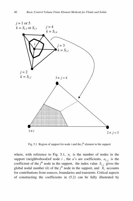
Basic Control Volume Finite Element Methods for Fluids and Solids
40
Fig. 5.1 Region of support for node i and the jth element in the support
where, with reference to Fig. 5.1, in is the number of nodes in the
support (neighborhood)of node i , the a’s are coefficients, j,ia is the
coefficient of the jth node in the support, the index value j,iS gives the
global nodal number (k) of the jth node in the support, and ib accounts
for contributions from sources, boundaries and transients. Critical aspects
of constructing the coefficients in (5.2) can be fully illustrated by
i
j = 4
k = Si,4
j = 1 or 5
k = Si,1 or Si,5
j = 2
k = Si,2
j = 3
k = Si,3
43 =≡ j
32 =≡ ji≡1
CVFEM Discretization and Solution
41
considering a single finite element in the support, see the lower part of
Fig. 5.1. The coefficient calculations in this given element will be
identical to the calculations used in all the other elements in the support.
Then, on aggregating the calculated coefficient and source contributions
from each element in turn, full specification of the coefficient and source
terms in (5.2) can be achieved.
5.2 Preliminary Calculations
Before the coefficients associated with the selected single element in Fig.
5.1 are determined some preliminary values need to be calculated and
stored.
The volume of the element (assuming unit depth) is given by
1
1
1
2
1
33
22
11
yx
yx
yx
Vele =
=2
2313212332 )xx(y)yy(x)yxyx( −+−+−
(5.3)
The contribution of the volume of this element (the 3rd
element in the
region of support) to the control volume associated with node i (shown as
the bold polygon in the upper image in Fig. 5.1 is
eleji VV
31= (5.4)
From Chapter 3 (Eq. (3.9)) the derivatives of the shape functions
(constant in the elements) are
eleyelex
eleyelex
eleyelex
V
)xx(
y
NN,
V
)yy(
x
NN
V
)xx(
y
NN,
V
)yy(
x
NN
V
)xx(
y
NN,
V
)yy(
x
NN
22
22
22
1233
2133
3122
1322
2311
3211
−=
∂
∂=
−=
∂
∂=
−=
∂
∂=
−=
∂
∂=
−=
∂
∂=
−=
∂
∂=
(5.5)

Basic Control Volume Finite Element Methods for Fluids and Solids
42
From (5.5) the components of the gradient
∂
φ∂
∂
φ∂=φ∇
y,
x
in the element are
332211 φ+φ+φ=∂
φ∂xxx NNN
x (5.6a)
and
332211 φ+φ+φ=∂
φ∂yyy NNN
y (5.6b)
With reference to Fig. 5.2 and moving in a counter-clockwise direction
around node i the change in x value, along face 1 in the element is
663
1231
xxxx f −−=∆
(5.7)
The change in y value is
663
1231
yyyy f −−=∆
(5.8)
The equivalent changes in x and y values along face 2 are respectively
663
1322
xxxx f ++−=∆
(5.9)
663
1322
yyyy f ++−=∆
(5.10)
The area of face 1 in the element (assuming unit depth) is
21
211 fff yxA
∆+∆= (5.11)
The area of face 2 is
22
222 fff yxA
∆+∆= (5.12)

CVFEM Discretization and Solution
43
Fig. 5.2 The faces of the control volume
The components of the unit normal (pointing out of the ith
control
volume) on face 1 (see Fig. 5.2) is
1
11
1
11
f
ffy
f
ffx
A
xn,
A
yn
∆−
=∆
= (5.13)
On face 2 the components are
1(i) 2
3
1(i) 2
3
x
∆
y
∆ n
x
∆
y
∆n
face 1
face 2

Basic Control Volume Finite Element Methods for Fluids and Solids
44
2
22
2
22
f
ffy
f
ffx
A
xn,
A
yn
∆−
=∆
= (5.14)
The value of the diffusivity at the mid-point of face 1 (indicated in Fig.
5.2) is
3122
2125
1125
13322111 κ+κ+κ=κ+κ+κ=κ ff ]NNN[ (5.15)
At the mid-point of face 2
3125
2122
1125
13322112 κ+κ+κ=κ+κ+κ=κ ff ]NNN[ (5.16)
The velocity components at the midpoint of face 1 are
321 12
2125
1251
xxxfx vvvv ++= (5.17a)
and
321 12
2125
1251
yyyfy vvvv ++= (5.17b)
On face 2
321 12
5122
1252
xxxfx vvvv ++= (5.18a)
and
321 12
5122
1252
yyyfy vvvv ++= (5.18b)
The volume flow (volume/time) out across face 1, in the direction of
the outward normal, is
11
11
11 ffyf
fxff xvyvAq
∆−∆=⋅= nv (5.19)
Across face 2
22
22
22 ffyf
fxff xvyvAq
∆−∆=⋅= nv (5.20)
Armed with these preliminary calculations the appropriate
coefficients in 5.2 can be calculated. This process is illustrated by
developing discrete forms of the advection-diffusion equation.
5.3 Steady State Diffusion
For steady state diffusion the governing equation is
CVFEM Discretization and Solution
45
0=⋅φ∇κ∫A
dAn (5.21)
Associating the domain of this integration with the area of the control
volume associated with node i (the bolded polygon in. Fig 5.1)
0
1
=⋅φ∇κ=⋅φ∇κ ∑ ∫∫=
i
j
n
j AA
dAdA nn (5.22)
where jA is the area of the control volume faces in the j
th element of the
support. Note that at an internal domain node the number of elements
and nodes in a support are equal. Equation (5.22) states that the net
diffusive flux into the ith control volume is zero.
Each term in the sum on the right-hand side of (5.22) can be
approximated using a midpoint integration rule. For the selected
triangular element in Fig. 5.1 this approximation leads to
21
213
ff
facefaceA
AA
dAdAdA
nn
nnn
⋅φ∇κ+⋅φ∇κ≈
⋅φ∇κ+⋅φ∇κ=⋅φ∇κ ∫∫∫
(5.23)
From the results in the previous section the following expansions can be
made
13322111
13322111
11111
fyyyf
fxxxf
fffff
x]NNN[
y]NNN[
xy
yx
A
∆φ+φ+φκ−
∆φ+φ+φκ=
∆∂
φ∂κ−∆
∂
φ∂κ=⋅φ∇κ n
(5.24)
and
23322112
23322112
22222
fyyyf
fxxxf
fffff
x]NNN[
y]NNN[
xy
yx
A
∆φ+φ+φκ−
∆φ+φ+φκ=
∆∂
φ∂κ−∆
∂
φ∂κ=⋅φ∇κ n
(5.25)
Substituting these expansions in (5.23) and using global indexing for the
unknown nodal field results in

Basic Control Volume Finite Element Methods for Fluids and Solids
46
4,3,
3
321 ii SSi
A
aaadA φφφφκ κκκ ++−≈⋅∇∫ n (5.26)
where
2322321311313
2222221211212
2122121111111
fyffxffyffxf
fyffxffyffxf
fyffxffyffxf
xNyNxNyNa
xNyNxNyNa
xNyNxNyNa
∆κ−∆κ+∆κ−∆κ=
∆κ−∆κ+∆κ−∆κ=
∆κ+∆κ−∆κ+∆κ−=
κ
κ
κ
(5.27)
The superscript ()κ is used to indicate that these values are the diffusive
contribution to the coefficients in the general form (5.2). These values
can be used to update the ith support coefficients through
κ
κ
κ
34,4,
23,3,
1
aaa
aaa
aaa
ii
ii
ii
+=
+=
+=
(5.28)
The updating form of (5.28) is used to indicate that contributions to a
given support coefficient can come from other elements in the support;
take care with this equation to recognize the distinction between indices
identifying support nodes and nodes in the selected triangular element,
e.g., 4,i() represents the 4th node in the support of node i (upper part of Fig
5.1 and ()3 represents the 3rd
node in the selected element (lower part of
Fig. 5.1).
5.4 Steady State Advection-Diffusion
For Steady State advection-diffusion the governing equation is
0=φ⋅−⋅φ∇κ ∫∫AA
dA)(dAn nv (5.29)
Associating the domain of this integration with the area of the control
volume for node i (the bolded polygon in Fig. 5.1) allows for the
expansion

CVFEM Discretization and Solution
47
φ⋅−⋅φ∇κ ∫∫n
AA
dA)(dAn nv
= 0
1
=φ⋅−⋅φ∇κ∑ ∫∫=
i
jj
n
j AA
dA)(dAn nv
(5.30)
This equation states that the net advective + diffusive flux into the ith
control volume is zero. Each term in the sum on the right-hand side of
(5.30) can be approximated using a midpoint integration rule. For the
selected triangular element in Fig. 5.1 this approximation leads to
21
21
3
3
33
ff
A
facefaceA
AA
A)(A)(dA
dA)(dA)(dA
dA)(dAn
φ⋅−φ⋅−⋅φ∇κ≈
φ⋅−φ⋅−⋅φ∇κ
=φ⋅−⋅φ∇κ
∫
∫∫∫
∫∫
nvnvn
nvnvn
nv
(5.31)
On expansion, the first term on the right-hand-side will generate the
diffusion coefficients given in (5.27), and the later terms can be written
in terms of the volume flow rates (see (5.19) and (5.20)) to arrive at
-
2211321
21
43
3
ffffSSi
ff
A
qqaaa
A)(A)(dA
,i,iφ−φ−φ+φ+φ−
=φ⋅−φ⋅−⋅φ∇κ
κκκ
∫ nvnvn
(5.32)
where the a’s are the diffusive coefficients given in (5.27). To move
forward we need to be able to approximate the face values of the
unknown scalar φ . An obvious choice is
3122
2125
1125
13322111 φ+φ+φ=φ+φ+φ=φ ff ]NNN[ (5.33a)
and
3125
2122
1125
23322112 φ+φ+φ=φ+φ+φ=φ ff ]NNN[ (5.33b)
This is equivalent to the central difference approximation for the
advective face value in the Control Volume Finite Difference Method. In
a similar manner to the FDCVM this choice can lead to a poorly
conditioned system in advection dominated problems (Patankar (1980)).
=
=

Basic Control Volume Finite Element Methods for Fluids and Solids
48
The first order avoidance measure for this problem is to employ an up-
wind approach, setting
<φ
>φ=φ
0
0
12
11
1f
f
fqif
qif (5.34a)
and
<φ
>φ=φ
0
0
23
21
2f
f
fqif
qif (5.34b)
This will always lead to well conditioned systems but can also induce
numerical dissipation (artificial diffusion). Similar concepts to those used
in CVFDM can be used to improve CVFEM performance for advection
dominated flows but due to the unstructured nature of the mesh they can
be a little trickier to implement, e.g., see Woodfield et al (2004).
If upwinding is used the last two terms in (5.32) can be replaced with
1 1 1 1 1 2max[ ,0] max[ ,0]f f f f
q q q− φ = − φ + − φ (5.35a)
and
2 2 2 1 2 2max[ ,0] max[ ,0]f f f f
q q q− φ = − φ + − φ (5.35b)
On making this replacement and gathering terms, we can write down the
following approximation for the advective + diffusive flux arriving into
the control volume across the faces located in element 3
43
3
332211
21
,i,i Su
Su
iu
ff
A
)aa()aa()aa(
A)(A)(dA
φ++φ++φ+−
=φ⋅−φ⋅−⋅φ∇κ
κκκ
∫ nvnvn
(5.36)
where the advective coefficients, identified with the superscripts ()u , are
given by
]0,max[
]0,max[
]0,max[]0,max[
23
12
211
f
u
f
u
ff
u
qa
qa
qqa
−=
−=
+=
(5.37)
These values can be used to update the ith support coefficients through
=
CVFEM Discretization and Solution
49
u
ii
u
ii
u
ii
aaaa
aaaa
aaaa
334,4,
223,3,
11
++=
++=
++=
κ
κ
κ
(5.38)
The updating form is used to account for contributions to the nodal
coefficients from other elements in the support. Again, as noted below
equation (5.28), take care to recognize the distinction between indices
identifying support nodes and nodes in the selected triangular element.
5.5 Steady State Advection-Diffusion with Source Terms
When source terms are present the governing equation is
0)( =⋅+⋅∇−∫ ∫∫V AA
dAdAdVQ φφκ nvn (5.39)
The discretization of the diffusive and advection terms (terms 2 and 3 on
the left hand side) are detailed in the two previous sections. Here we just
focus on the source term. If the volume V is associated with the control
volume around node i in Fig. 5.1 this term can be written
∑ ∫∫=
= elements
1j VV
dVQdVQj
ii
(5.40)
where the sum is over the elements in the region of support for node i
and j
iV is the volume contribution to the control volume from the jth
element in the support, see (5.4).
5.5.1 Volume source terms
If Q(x,y) is a volume source term (quantity/volume-time) then the right
hand side can be approximated by a one-point integration to arrive at
ii
j V
VQdVQj
i
≈∑ ∫=
elements
1
(5.41)
Basic Control Volume Finite Element Methods for Fluids and Solids
50
where )y,x(QQ iii = is the value of the source evaluated at the location
of node i and
∑=
=elements
j
jii VV
1
is the volume of the ith control volume. This approach of approximating
the source is referred to as nodal lumping and is effectively a one-point
integral centered on the node point of the given control volume. An
alternative is to perform separate volume integrals for each element on
the right-hand-side of (5.40). The domain for such an integral is the
shaded region illustrated in the lower part of Fig 5.1 and can be
performed using a Gauss quadrature. This approach, referred to as a
consistent approach, may have more accuracy if Q(x,y) changes rapidly.
Nodal lumping, however, results in better convergence properties for the
system (5.2) and is often the preferred approach in CVFEM
5.5.2 Source linearization
When Q(x,y) is a volume source term the full discrete equation
corresponding to (5.39) is
∑=
+φ=φi
j,i
n
j
iiSj,iii VQaa
1
(5.42)
It is possible that, in the general case, )y,x(QQ iii = will be a function
of the nodal unknown value iφ . Thus (5.42) could form a non-linear
system and its solution could require iteration. A crude approach simply
calculates )y,x(QQ iii = based on the best available estimates for
iφ (i = 1.. n) and then solve the system (5.42) to arrive at a better
estimates for iφ . If the source is highly non-linear, however, convergence
of this approach could be very slow or non-existent. Computational
solution performance can be dramatically improved by linearizing the
source term
ii BiCii QQVQ +φ−= (5.43)
CVFEM Discretization and Solution
51
In (5.43) BC QQ and can still be functions of the nodal values ofφ but
to be effective it is essential that 0 >CQ throughout the calculation; if
(5.42) is written as the system bφA = a positive value 0 >CQ will
increase the magnitude of the diagonal elements of A and improve the
conditioning of the system.
5.5.3 Line source
If the source is a line source located at )y,x( kkk =x ,
)(QQ k xx −δ= ℓ (5.44)
where ℓ
Q (quantity/time-unit depth) is independent of φ , and
)( k xx −δ , the Dirac delta function, has the properties
=∞
≠=−δ
k,
,)(
xx
xxxx
kk
0 (5.45a)
∫∞
∞−
=−δ 1)( k xx (5.45b)
In the case that an internal node i is located on kik , xxx = i.e., , see
Fig. 5.3a
ℓQdVQ
iV
=∫ (5.46)
and the terms in the linearized source are
lBC QQ,Qii
== and 0 (5.47)
If the node i is located on an insulated (symmetry) boundary, however,
see Fig 5.3b, the source term is
ℓQdVQ
iVπ
θ=∫ 2
(5.48)
where θ is the angle (radians) between the boundaries joining at node i;
this results in the settings

Basic Control Volume Finite Element Methods for Fluids and Solids
52
Fig. 5.3 Treatment of line source; a. node i located inside domain, b. node i located on
insulated boundary
lBC QQ,Qii π
θ==
2 and 0 (5.49)
5.6 Coding Issues
The discrete form of the steady-state advection-diffusion equation (5.39)
is
∑=
+φ=φ+i
ij,ii
n
j
BSj,iiCi Qa]Qa[
1
(5.50)
The work in prior parts of this chapter have shown how the terms in this
equation can be calculated using CVFEM. At this point is worthwhile to
summarize these calculations by outlining how a computational code to
evaluate the terms in (5.50) can be constructed.
Using the data structure and nomenclature outlined in Chapter 4.
An outer loop calls at each of the n nodes in the mesh, n..i 1= .
-- At each node i values for the support volume ,Vi and the coefficients
ii BC Q,Q and )n..j(aa ij,i,i 1= are set to a default value of zero.
Q
Q θ
a. b.
i i
CVFEM Discretization and Solution
53
-- Each node i is identified as an internal node point ( 011 ≠=+ ,in,i SSi
) or
a boundary node point ( 01 =+in,iS ) and a loop counter is set to
inloop = at internal nodes or 1−= inloop at boundary nodes.
-- A loop is made over the nodes in the support of node i, loopj ..1= .
[Note: the value of j in this loop can be associated with the jth element
in the support of node i. Internal node supports will always have the
same number of elements as support nodes, hence the setting inloop = .
Boundary node supports will always have one less element than support
node, hence the setting 1−= inloop ]
----At each value of j in the loop:
----The coordinates of the vertices of the jth element are extracted
1,,
1,,
321
321
,,
,,
+
+
===
===
jiji
jiji
SSi
SSi
yyyyyy
xxxxxx
----The preliminary data is calculated, (5.3) to (5.20), and stored
----The control volume is updates as j
iii VVV +=
----The diffusive coefficients kkka,a,a 321 are calculated (5.27) and stored
----The advective coefficients uuu
aaa 321 ,, are calculated (5.37) and
stored
---- The support coefficients are updated from
u
j,ij,i
uii
aaaa
aaaa
22
11
++=
++=
κ
κ
=++=
≠++=
κ
κ+
iu
j,i,i
iu
j,ij,i
njiaaaa
njaaaa
f
if
331
331
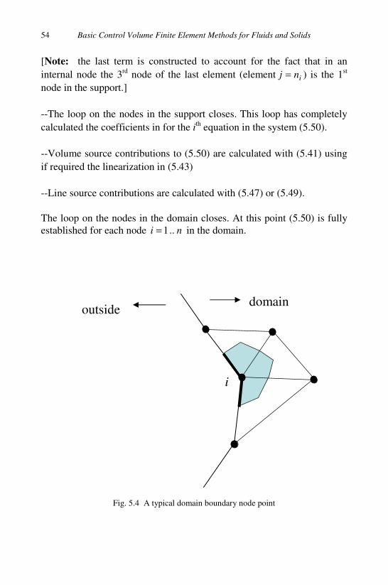
Basic Control Volume Finite Element Methods for Fluids and Solids
54
[Note: the last term is constructed to account for the fact that in an
internal node the 3rd
node of the last element (element inj = ) is the 1st
node in the support.]
--The loop on the nodes in the support closes. This loop has completely
calculated the coefficients in for the ith equation in the system (5.50).
--Volume source contributions to (5.50) are calculated with (5.41) using
if required the linearization in (5.43)
--Line source contributions are calculated with (5.47) or (5.49).
The loop on the nodes in the domain closes. At this point (5.50) is fully
established for each node n..i 1= in the domain.
Fig. 5.4 A typical domain boundary node point
i
domain outside

CVFEM Discretization and Solution
55
5.7 Boundary Conditions
Up to this point, the terms in the discrete form for a steady state
advection-diffusion equation have been fully defined. Before a real
problem can be solved, however, appropriate boundary conditions need
to be applied. This step requires the modification of (5.50) with the
addition of extra terms for the nodes i that are located on a domain
boundary. Consider a typical boundary node, Fig 5.4, located on the jth
node ( k,Bnj ≤≤1 ) of the ( segnk ≤≤1 ) domain boundary segment.
Recall from the data structure given in Chapter 4, that segn is the number
of segments of the domain boundary (arranged counterclockwise around
the domain boundary), k,Bn is the number of nodes on the kth
segment,
and the counter j sequentially counts the nodes in the counterclockwise
direction. The discrete equation associated with the node i in Fig. 5.4 is a
balance over the shaded polygonal control volume. Key parts of this
balance are the fluxes crossing the control volume faces. In previous
sections the diffusive and convective fluxes across the faces that do not
belong to the domain boundaries have been evaluated. Contributions
across control faces that coincide with the domain boundary—the bold
lines in Fig. 5.4—have, however, not been determined.
5.7.1 Face area calculations
To provide a general treatment for boundary conditions some
preliminary calculation of the boundary face areas associated with each
node j in a given boundary segment are required. Figure 5.5 shows a
schematic of the kth (k = 3) boundary, indicating the data structure.
Assuming unit depth, the face area associated with any node j of the
boundary segment highlighted in Fig 5.5 is given by
−≤≤+=
k,Bn
k.Bjjj,k
Lower
nj,LowerUpper
Upper
A 12
1
(5.51)

Basic Control Volume Finite Element Methods for Fluids and Solids
56
Fig. 5.5 A domain boundary segment with three sequential points detailed
where
2
12
121
21
212
1
)yy()xx(Lower
,)yy()xx(Upper
jjjjj
jjjjj
−−
++
−+−=
−+−=
The first and last lines on the right-hand side of (5.51) account for the
first and last node on the boundary segment. This treatment assumes that
there are at least two boundary segments—i.e., at least two contiguous
regions of the domain boundary where different boundary conditions are
applied. In cases where only one boundary condition is applied (e.g., a
constant value over the whole boundary) the condition of a two-segment
boundary can be artificially imposed.
The coding to calculate the boundary face values can be as follows:
Loop over the boundary segments kn..k 1=
--Loop over the nodes on segment k, k,Bn..j 1=
----Associate local boundary coordinates with global coordinates, i.e.,
. . . .
. . . .
k = 1
k = 4
k =3
k = 2
j = 1
j = nB,3
j
j-1
j+1
i = Bk,j
.
.
.
. . . .
. . . .
k = 1
k = 4
k =3
k = 2
j = 1
j = nB,3
j
j-1
j+1
i = Bk,j
.
.
.
CVFEM Discretization and Solution
57
k,BBjBj
k,BBjBj
BjBj
nj,yy,xx
nj,yy,xx
j,yy,xx
j,kj,k
j,kj,k
j,kj,k
<==
<≤==
>==
++
−−
++
−−
11
11
11
11
1
1
----Calculate j,kA from (5.51)
--Close loop on j
Close loop on k
5.7.2 Convective condition
A general treatment for boundary conditions can be achieved by
considering the convective boundary condition
∫∫ φ−φ=A
amb
A
in dA)(hdAq (5.52)
This states that the net flux (quantity/area-time) entering the domain
across the area A is specified by a transfer coefficient 0≥h and an
ambient value of the field variable ambφ . When the domain of the
integral, A, is associated with the face areas of node i, coinciding with the
domain boundary, this is the flux value that needs to be added to the
right-hand side of (5.50). Using a nodal lumping approach the integral
on the right of (5.52) can be approximated as
ambBiC
A
amb hBBdA)(hii
φ+φ−≈φ−φ∫ (5.53)
where
j,kambBj,kC AhB,hABii
φ=>= 0 (5.54)
and the index j,kBi ≡ . In this way the convective boundary condition
can be added by extending (5.50) to
∑=
++φ=φ++i
iij,iii
n
j
BBSj,iiCCi BQa]BQa[
1
(5.55)
This can be achieved by the following coding:
Basic Control Volume Finite Element Methods for Fluids and Solids
58
Loop over the nodes in the domain, n..i 1= , setting
0 and0 ==ii BC BB
Loop over the boundary segments kn..k 1=
--Loop over the nodes on segment k, k,Bn..j 1=
---- Calculate global node index associated with node j, i.e., j,kBi =
----Calculate andii BC BB from (5.54)
--Close loop over j segment
Close loop on boundary segments k
5.7.3 Generalization of the convective boundary condition
By appropriate choice of the value of h and ambφ the definition of the
boundary source terms,ii BC BB and , can be effectively used to model a
range of possible boundary conditions.
Convective Boundary: Clearly a finite setting of h and ambφ will
provide, by definition, a convective boundary condition.
Insulated Boundary: A setting of h = 0 and a finite value of ambφ will
provides an insulated –no-flow—boundary. The only coding required for
this boundary condition is to ensure that, for nodes i on an insulated
boundary, the settings 0 and0 ==ii BC BB are made. Note this is the
default condition arising from CVFEM procedures leading to the discrete
from (5.50).
Fixed Value Boundary: A setting of 1610=h (a large number) and
valueamb φ=φ (a prescribed value) ensures that at the boundary node i in
question, the terms valueCBC iiiBBB φ= and will dominate, essentially
reducing (5.55) to

CVFEM Discretization and Solution
59
ii BiC BB ≈φ (5.56)
On noting that valueCB iiBB φ= , this choice forces the fixed value
(Dirichlet) condition valuei φ≈φ . In practice this prescribed-value
boundary condition can be obtained with a minimum of coding. All that
it required is that, for nodes i on a fixed value boundary, the settings 1616 10 and10 ×== valueBC ii
BB φ are made.
Fixed Flux Boundary: Finally a setting of 1610−=h (a small value) and
hqinamb /=φ , where inq is a prescribed flux into the domain, will
essentially force the settings inj,kBC qABBii
=≈ and0 , such that, at
global node i corresponding to node j on the prescribed flux boundary
segment k, (5.55) takes the required form
∑=
++φ=φ+i
ij,ii
n
j
inj,kBSj,iiCi qAQa]Qa[
1
(5.57)
5.8 Solution
The following sequential steps leads to a fully defined system of discrete
equations, (5.55), for a given steady-state advection-diffusion problem:
-Calculation of diffusive coefficients
-Calculation of advective coefficients
-Treatment of sources
-Treatment of boundary conditions
The final step is to solve this equation (5.55) and determine the nodal
field values )n..i(,i 1=φ . There is a plethora of possible solution
techniques that could be applied. A flexible, if not necessarily efficient,
approach is a point wise Gauss-Seidel iteration which writes (5.55) as
1
1
−
=
++φ=φ++ ∑
r,rn
j
BBSj,iriCCi
i
iij,iiiBQa]BQa[ (5.58)
Basic Control Volume Finite Element Methods for Fluids and Solids
60
where the superscript r() indicates the r
th approximation and the
subscript 1,[] −rr indicates that the item in brackets is evaluated with the
currently available approximation. Starting from an initial guess for the
nodal field— )n..i(,i 100 ==φ is often a reasonable default—(5.58) is
solved to provide an updated values )n..i(,i 11 =φ . In a subsequent step,
these value can be used on the right hand side of (5.58) to obtain the
updates )n..i(,i 12 =φ . This iteration cycle continues until convergence,
defined by
tolerancespecified11 <=φ−φ −)n..i(,max
ri
ri (5.59)
The equation in (5.58) could be non-linear—i.e., the coefficients (a),
source terms (Q) and boundary conditions (B) could be functions of the
unknown iφ . In this case under-relaxation may be required to solve
(5.58). The point solution is rewritten as
++
φ++−
++φ
ω+φ=φ
−
−
=−
∑
]BQa[
]BQa[BQa
ii
ii
i
iij,i
CCi
riCCi
r,rn
j
BBSj,i
ri
ri
1
1
11
(5.60)
where 10 ≤ω< is a relaxation factor. Note that the numerator in the
brackets on the right hand side determines, for the current field estimates,
the miss-match between the left and the right hand side of (5.55). Hence
the term in brackets can be viewed as a correction, improving the
estimate from 1−φri to r
iφ ; note, on convergence this correction
vanishes. The convergence of (5.60) is controlled by the choice of ω , if
too large a value is chosen the point iteration may diverge, if too small
convergence may be very slow (require multiple iterations). The
optimum value is usually found by trial and error. In this respect it is
worth noting that if the system (5.55) is linear (or close to linear) the
optimum value may be 1≥ω , referred to as over-relaxation.
CVFEM Discretization and Solution
61
Appropriate coding for the solver is as follows—throughout this code
the best available value of the field variable r,ri
1−φ is stored as iφ and
the updated value riφ is stored as up
iφ .
An initial guess is assigned to the field value )n..i(,i 10 ==φ
Values for a convergence tolerance tol, an under-relaxation factorω , and
maximum number of iterations maxit are prescribed. A default for the
maximum difference is set as max-diff = 0
A loop is made over an iteration counter ..1=r maxit
--For each choice of r, a loop is made over the domain nodes
ni ..1=
----Looping over the nodes, inj ..1= , in the ith
region of support
------The value ∑=
φi
j,i
n
jSj,ia
1
of is calculated and stored.
----Close Loop on j
----Update the nodal value of ri
upi φ=φ from (5.60)
----If >− i
up
i φφmax max-diff set max-diff = iupimax φ−φ
----Set current best nodal value upii φ=φ
--Close Loop on i
--If max-diff<tol terminate iterations
Close Loop on r
If r = maxit, print a warning that convergence has not been achieved

Basic Control Volume Finite Element Methods for Fluids and Solids
62
5.9 Handling Variable Diffusivity
In the treatment provided above, it is assumed that the diffusivity is a
continuous and known function of space ( )y,xf=κ . In this way nodal
values iκ can be calculated a-priori and values at any point in an element
can be found through the shape function interpolation (5.15) and (5.16).
There are two important cases when this treatment cannot be used.
5.9.1 A conjugate problem
A conjugate problem is one in which two or more regions in the domain
have distinct values for the diffusivity and there is a “jump” in the
diffusivity across the interface between the regions, e.g., heat conduction
in a liquid metal contained in a mold. If the location of the sub-regions
are fixed and known, the best way to deal with this problem is to
construct the mesh so that any given element falls in one and only one
region, see Fig (5.6). In this way, since the CVFEM is constructed from
the individual triangular elements there is no ambiguity in calculating the
face diffusivities in a given element.
Fig. 5.6 Suggested mesh arrangement for a conjugate diffusion problem
Region 1
Region 2
constantconstant 21 =κ≠=κ

CVFEM Discretization and Solution
63
5.9.2 Diffusivity a function of field variable
In many models and problems the diffusivity is a function of the
unknown field, i.e., ( )φ=κ f . While the basic treatment outlined in §5.3
will work for this case, the resulting system of equations (5.55) will be
non-linear. This will require an iterative solution with the full
recalculation of the CVFEM diffusive coefficients at each step. An
alternative, more efficient approach for this case is a follows. If the
diffusive contributions to the coefficients are separated and stored
separately, the discrete equation (5.55) can be rewritten as
∑∑==
++φ+φ−φ
=φ++
i
iij,i
i
j,i
ii
n
j
BBSu
j,i
n
j
ikiS
kj,i
iCCui
BQaaa
]BQa[
11
(5.61)
For a given element, on noting the properties of the shape function and
its derivatives,
yyyxxx NNNNNNNNN 321321321 and1 +=−+=−⇒+=− ,
it follows from (5.27) that in an element, kkkaaa 321 += and that in a
region of support,
∑=
=in
j
kj,i
ki aa
1
In this way, on first calculating the diffusion coefficients assuming 1=κ ,
a version of (5.61), accounting for the variable diffusivity, is given by
Fig. 5.7 Diffusivity at faces meeting on side i-j
i
j
j,ik
i
j
j,ik
=

Basic Control Volume Finite Element Methods for Fluids and Solids
64
∑∑==
++φ+φ−φκ
=φ++
i
iij,i
i
j,i
ii
n
j
BBSu
j,i
n
j
iSk
j,ij,i
iCCui
BQa)(a
]BQa[
11
(5.62)
where the diffusivity acting on the two faces joining on the element side
connecting node i and j, see Fig 5.7, is
2
)()(j,iSi
j,i
φκ+φκ=κ (5.63)
Equation (5.62) can be readily manipulated into the iterative form
++κ+
φ+++−
++κ+
++φκ+
ω+φ=φ
∑
∑
∑
=
−
=
−
=
−
]BQaa[
]BQaka[
]BQaa[
BQ)aa(
ii
i
ii
ii
i
i
iij,i
CCki
n
j
j,iui
riCC
kj,ij,i
ui
CCki
n
j
j,iui
r,rn
j
BBSk
j,ij,iu
j,i
ri
ri
1
1
1
1
1
1 (5.64)
Although this is more involved than the basic iterative scheme in (5.60)
the additional computations in forming this equation during the iteration
are minimal. At node i during the rth iteration, perform the following
steps
----Loop over the nodes, inj ..1= , in the ith region of support
------**Calculate j,iκ from (5.63)
------Calculate and store the value ∑=
φκ+i
j,i
n
jS
kj,ij,i
uj,i )aa(
1
=

CVFEM Discretization and Solution
65
------**Calculate the sum ∑=
κin
j
j.i
1
----Close Loop on j
The only additional calculations from the basic iteration are marked with
(**). This additional calculation is much less intensive that the
alternative of reforming the diffusive coefficients on each iterative step.
5.10 Transients
From the above the net flow rate of quantity into the control volume
around node i can be approximated as
∑
∑ ∫∫∫
=
=
++φ+φ++−≈
φ⋅−⋅φ∇κ+=
i
iij,iii
i
jji
i
n
j
BBSj,iiCCi
n
j AAV
BQa]BQa[
dA)(dAdVQNet
1
1
nvn
(5.65)
In a steady state problem this flow rate will be identically zero. In a
transient problem, however, it will result in a change in storage of the
quantity in the control volume, i.e.,
∫ =φ
iV
iNetdVdt
d (5.66)
Using nodal lumping for the volume integration and finite difference in
time this equation can be used to evaluate the nodal field values at time
tt ∆+ in terms of the nodal field values at time t ,
( ) ]NetNet[tVVnewiiii
newii θ+θ−∆+φ=φ 1 (5.67)
where t∆ is a time step and the superscript ()new
indicates evaluation at
time tt ∆+ . The parameter 10 ≤θ≤ is a user-defined weighting factor,
used to approximate the net flow into control volume i during the time

Basic Control Volume Finite Element Methods for Fluids and Solids
66
interval [ ]tt,t ∆+ , in terms of the net flows at the beginning and end of
the time step. Neglecting, for now, contributions from the boundaries and
sources, the resulting discrete equations for three choices of θ are:
Fully Implicit 1=θ :
φ−φ∆+φ=φ ∑
=
i
j,i
n
j
newii
newSj,iii
newii aatVV
1
(5.68)
The advantage of this choice is that it is unconditionally stable—i.e., for
any choice of time step errors (induced or inherent) will not grow. The
downside is that a system of equations needs to be solved to obtain the
field values at the new time step )n..i(newi 1=φ .
Crank-Nicolson 5.=θ :
φ−φ
∆+
φ−φ
∆+φ=φ ∑∑
==
i
j,i
i
j,i
n
j
iiSj,i
n
j
newii
newSj,iii
newii aa
taa
tVV
11 22
(5.69)
This un-conditionally stable scheme also requires a system solution.
Unlike the 1st order in time, fully implicit method, however, the Crank-
Nicolson is 2nd
order in time (i.e., time errors scale with 2t∆ . By the way
there is no h in Nicolson, see Crank and Nicolson (1947).
Fully Explicit 0=θ :
φ−φ∆+φ=φ ∑
=
i
j,i
n
j
iiSj,iiinewii aatVV
1
(5.70)
This choice can be used to directly update the new time level values from
the current time values without solution of a system of equations. This,
however, comes at the price of a restriction on the time step size to
ensure stability. The solution of (5.70) is likely to become unstable (error
grow as the solution advances) if the net coefficient for iφ becomes
negative. This requires that the time step is chosen such that
CVFEM Discretization and Solution
67
)n..i(,a
Vmint
i
i =
<∆ (5.71)
If a fine grid is used this value could be prohibitively small, i.e., the
advance of time could be too slow to reach a practical value within
reasonable computational resources. In many cases, however, the
drawback for using a small time step is offset by the ability to solve
(5.70) without iteration. Driven by its simplicity and flexibility of
modeling complex non-linear terms the explicit time integration
approach is the preferred choice in this work.
When sources and boundary condition treatments are added the
explicit scheme (5.70) can be written as
iii
i
j,ii BiCB
n
j
iiSj,iiinewici BQQaatV)BV( +
φ−+φ−φ∆+φ=φ+ ∑
=1
(5.72)
The addition of the source term in (5.72) could require a further
reduction in the time step to retain positive coefficients and stability, i.e,.
)n..i(,Qa
Vmint
iCi
i =
+<∆
Further, the boundary treatment in (5.72) allows for an insulated
boundary on setting 0 and0 ==ii BC BB and a fixed value boundary on
setting valueCBC iiiBBB φ== and1016
.
The coding for one time step of the explicit scheme is very
straightforward.
The coefficients, source terms, and boundary treatments (fixed or
insulated) are all calculated by the steps outlined previously.
An appropriate time step is chosen.
++A loop is made over the domain nodes ni ..1=
-- Looping over the nodes, inj ..1= , in the ith region of support

Basic Control Volume Finite Element Methods for Fluids and Solids
68
---- The value ∑=
φi
j,i
n
jSj,ia
1
of is calculated and stored.
-- Close loop on j
-- The update new time value at node i is found directly from (5.70)
++Close loop on i
[note In solving over multiple time steps up to the simulation end time,
maxtime, the loop above, denoted by ++, is inserted in an outer time
loop]
timmax..itim 1=
++
++
Close loop on itim
5.11 Summary
At this point the key steps in a CVFEM discretization and solution of the
advection-diffusion equation (ADE) have been provided. The differences
between the CVFEM treatment of the ADE and treatments for solid and
fluid mechanics problems are essentially in the details. Hence, the
information provided in this chapter also enables the CVFEM treatments
of solid and fluids problems.
69
Chapter 6
The Control Volume Finite Difference Method
To provide a contrast with the CVFEM a brief overview of control
volume finite difference methods (CVFDM) is provided.
6.1 The Task
At this point it is very worthwhile to provide a brief overview of control
volume finite difference methods (CVFDM). This serves two purposes:
1. It reinforces some of the key concepts of CVFEM
2. It provides an alternative to CVFEM; an alternative that in some cases
may prove to be an easier and more convenient solution approach for the
problem at hand
In the presentation of the CVFDM we will focus on the two-
dimensional steady state advection diffusion equation, in integral form
0=φ⋅−⋅φ∇κ+ ∫∫∫AAV
dA)(dAdVQ nvn (6.1)
The central task is to write this equation in a discrete form—similar in
nature to the CVFEM discrete equation (6.55).
6.2 CVFDM Data Structure
The key components of the data structure for a CVFDM discretization
are shown in Fig 6.1. Note, for the case shown

Basic Control Volume Finite Element Methods for Fluids and Solids
70
Fig. 6.1 Data structure for CVFDM
1. the rectangular control volumes (bold lines) fit the solution domain,
2. the nodes, located at the control volume centers, are on a structured
mesh (dashed lines), i.e., a node location can be located with a row (i)
column (j) index ()i,j ,
3. the faces of the control volume around node ()i,j are labeled n(orth),
w(est), s(outh), and e(ast),
4. the unit normal on the control volume faces are
),();,();,();,( eswn 01010110 =−=−== nnnn
5. the areas of these faces (assuming unit depth) are
j,iwej,isn xAA,yAA ∆==∆==
n
s
w een
nn
wn
j,ix∆
j,iy∆
i,j i,j+1
i+1,j
i,j-1
i-1,j sn
j=1
i = 1
j=col.
i = row
The Control Volume Finite Difference Method
71
6. the volume of the control volume around node ()i,j is
j,ij,ij,i yxV ∆×∆=
7. the distance between node ()i,j and its neighbors to the to the north,
west, south and east are, respectively
22
22
11
11
+−
−+
∆+∆=δ
∆+∆=δ
∆+∆=δ
∆+∆=δ
j,ij,ie
j,ij,is
j,ij,iw
j,ij,in
xx,
yy
xx,
yy
In nodes adjacent to domain boundaries these values measure the
distance from the node to the respective boundary.
With the data structure of Fig 6.1 the discrete equation for (6.1) will
take the form
ijBj,iej,isj,iwj,inj,iCp BQaaaa]Qa[ijijijijijijij
++φ+φ+φ+φ=φ+ +−−+ 1111
(6.2)
i.e., for each node ()i,j in the domain, 5 coefficients )a,a,a,a,a( eswnp ,
associated with the node and its neighbors, linearized source terms
)QQ(ijij BC and , and a single boundary term ijB will be identified.
6.3 Coefficients and Sources
When the domains of integration in (6.1) are associated with the node ()i,j
the governing equation can be written as
∑ ∫∫∫
∫∫∫
=
⋅−⋅∇+
=⋅−⋅∇+
eswnk AAV
AAV
kkji
dAdAdVQ
dAdAdVQ
,,,
)(
)(
,
φφκ
φφκ
nvn
nvn
(6.3)
Employing midpoint integration rules the right hand side of (6.3) can be
approximated by
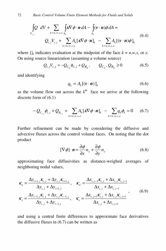
Basic Control Volume Finite Element Methods for Fluids and Solids
72
∑∑
∑ ∫∫∫
==
=
⋅−⋅∇+
≈⋅−⋅∇+
eswnk
kk
eswnk
kkjiji
eswnk AAV
AAVQ
dAdAdVQ
kkji
,,,,,,
,,
,,,
])[(][
)(
,
φφκ
φφκ
nvn
nvn
(6.4)
where []k indicates evaluation at the midpoint of the face k = n,w,s, or e.
On using source linearization (assuming a volume source)
0≥+φ−=ijijijij BCBj,iCj,ij,i Q,Q,QQVQ (6.5)
and identifying
kkk Aq ])[( nv ⋅= (6.6)
as the volume flow out across the kth face we arrive at the following
discrete form of (6.1)
0][,,,,,,
, ,,=−⋅∇++− ∑∑
== eswnk
kk
eswnk
kkBjiC qAQQjiji
φφκφ n (6.7)
Further refinement can be made by considering the diffusive and
advective fluxes across the control volume faces. On noting that the dot
product
yx ny
nx ∂
∂+
∂
∂=⋅∇
φφφ n][ (6.8)
approximating face diffusivities as distance-weighed averages of
neighboring nodal values,
1,,
1,,,1,
,1,
,1,,,1
1,,
1,,,1,
,1,
,1,,,1
,
,
+
++
−
−−
−
−−
+
++
∆+∆
∆+∆=
∆+∆
∆+∆=
∆+∆
∆+∆=
∆+∆
∆+∆=
jiji
jijijiji
e
jiji
jijijiji
s
jiji
jijijiji
w
jiji
jijijiji
n
xx
xx
yy
yy
xx
xx
yy
yy
κκκ
κκκ
κκκ
κκκ
, (6.9)
and using a central finite differences to approximate face derivatives
the diffusive fluxes in (6.7) can be written as
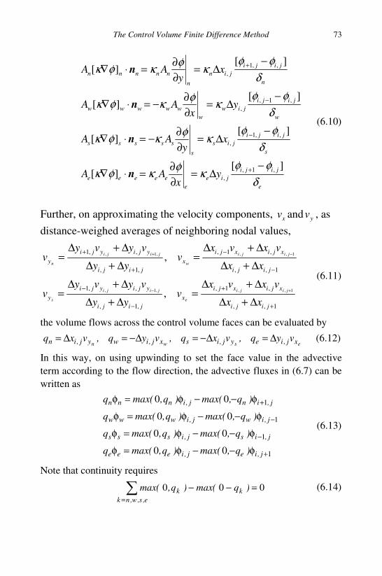
The Control Volume Finite Difference Method
73
e
jiji
jie
e
eeeee
s
jiji
jis
s
sssss
w
jiji
jiw
w
wwwww
n
jiji
jin
n
nnnnn
yx
AA
xy
AA
yx
AA
xy
AA
δ
φφκ
φκφκ
δ
φφκ
φκφκ
δ
φφκ
φκφκ
δ
φφκ
φκφκ
][][
][][
][][
][][
,1,
,
,,1
,
,1,
,
,,1
,
−∆=
∂
∂=⋅∇
−∆=
∂
∂−=⋅∇
−∆=
∂
∂−=⋅∇
−∆=
∂
∂=⋅∇
+
−
−
+
n
n
n
n
(6.10)
Further, on approximating the velocity components, yx vv and , as
distance-weighed averages of neighboring nodal values,
1,,
,1,
,1,
,,1
1,,
,1,
,1,
,,1
1,,,1,
1,,,1,
,
,
+
+
−
−
−
−
+
+
∆+∆
∆+∆=
∆+∆
∆+∆=
∆+∆
∆+∆=
∆+∆
∆+∆=
+−
−+
jiji
xjixji
x
jiji
yjiyji
y
jiji
xjixji
x
jiji
yjiyji
y
xx
vxvxv
yy
vyvyv
xx
vxvxv
yy
vyvyv
jiji
e
jiji
s
jiji
w
jiji
n
(6.11)
the volume flows across the control volume faces can be evaluated by
eswn xj,ieyj,isxj,iwyj,in vyq,vxq,vyq,vxq ∆=∆−=∆−=∆= (6.12)
In this way, on using upwinding to set the face value in the advective
term according to the flow direction, the advective fluxes in (6.7) can be
written as
1
1
1
1
00
00
00
00
+
−
−
+
φ−−φ=φ
φ−−φ=φ
φ−−φ=φ
φ−−φ=φ
j,iej,ieee
j,isj,isss
j,iwj,iwww
j,inj,innn
)q,max()q,max(q
)q,max()q,max(q
)q,max()q,max(q
)q,max()q,max(q
(6.13)
Note that continuity requires
000 =−−∑= e,s,w,nk
kk )qmax()q,max( (6.14)

Basic Control Volume Finite Element Methods for Fluids and Solids
74
On substituting (6.13) and (6.10) in (6.4), gathering terms and using
(6.14), the coefficients in (6.2) can be readily identified
∑=
=
−+δ
∆κ=−+
δ
∆κ=
−+δ
∆κ=−+
δ
∆κ=
e,s,w,nk
kp
ee
j,iees
s
j,ins
ww
j,iwwn
n
j,inn
ijij
ijij
ijij
aa
)qmax(y
a),qmax(x
a
)qmax(y
a),qmax(x
a
00
00
(6.15)
6.4 Boundary Conditions
Equation (6.7) and (6.15) respectively define the source terms and
coefficients in the CVFDM discrete form, (6.7), of the steady state
advection diffusion equation (6.1). To fully define the equation,
however, specification of the source term ijB needs to be made. The
default setting for this term is 0=ijB . A finite value is only required at
node points located in control volumes that share at least one face with a
domain boundary.
6.4.1 Insulated (no-flow) boundary
If the domain boundary is an insulated (no-flow) boundary the default
value 0=ijB is retained. In addition the control volume face coefficient
associated with the domain boundary is also set to zero. For example, if
the NORTH domain boundary is an insulated boundary the coefficient
setting 0=ijna is made; note this setting must be reflected in the
calculation of the node point coefficient
∑=
=e,s,wk
kp ijijaa (6.16)
6.4.2 Fixed value boundary
If the domain boundary (NORTH say) is a fixed value boundary
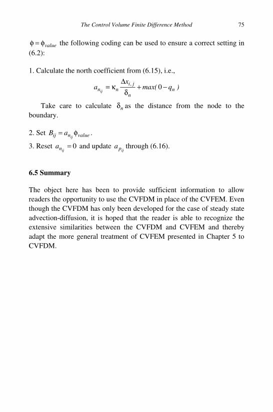
The Control Volume Finite Difference Method
75
valueφ=φ the following coding can be used to ensure a correct setting in
(6.2):
1. Calculate the north coefficient from (6.15), i.e.,
)qmax(x
a nn
j,innij
−+δ
∆κ= 0
Take care to calculate nδ as the distance from the node to the
boundary.
2. Set valuenij ijaB φ= .
3. Reset 0=ijna and update
ijpa through (6.16).
6.5 Summary
The object here has been to provide sufficient information to allow
readers the opportunity to use the CVFDM in place of the CVFEM. Even
though the CVFDM has only been developed for the case of steady state
advection-diffusion, it is hoped that the reader is able to recognize the
extensive similarities between the CVFDM and CVFEM and thereby
adapt the more general treatment of CVFEM presented in Chapter 5 to
CVFDM.
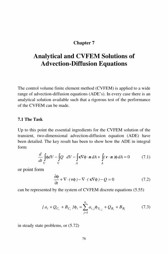
76
Chapter 7
Analytical and CVFEM Solutions of
Advection-Diffusion Equations
The control volume finite element method (CVFEM) is applied to a wide
range of advection-diffusion equations (ADE’s). In every case there is an
analytical solution available such that a rigorous test of the performance
of the CVFEM can be made.
7.1 The Task
Up to this point the essential ingredients for the CVFEM solution of the
transient, two-dimensional advection-diffusion equation (ADE) have
been detailed. The key result has been to show how the ADE in integral
form
0=φ⋅+⋅φ∇κ−−φ ∫∫∫∫AAVV
dA)(dAdVQdVdt
dnvn (7.1)
or point form
0=−φ∇κ⋅∇−φ⋅∇+∂
φ∂Q)()(
tv (7.2)
can be represented by the system of CVFEM discrete equations (5.55)
∑=
++φ=φ++i
iij,iii
n
j
BBSj,iiCCi BQa]BQa[
1
(7.3)
in steady state problems, or (5.72)

Analytical and CVFEM Solutions of Advection-Diffusion Equations
77
iii
i
j,ii BiCB
n
j
iiSj,iiinewici BQQaatV)BV( +
φ−+φ−φ∆+φ=φ+ ∑
=1
(7.4)
in transient problems; where the nodal values iφ and j,iSφ are located at
the vertices of an unstructured mesh of linear triangular finite elements.
The task at hand is to test and validate solutions of ADE’s based on these
discretizations. Access to test advection diffusion problems that admit
analytical solutions in is invaluable in fulfilling this task. Such problems
not only provide a measure of the accuracy of the solution scheme
developed but also provide a “safety net” that prevents conceptual and
coding errors.
7.2 Choice of Test Problems
In Cartesian coordinate systems, while there are a variety of solutions
available for the one-dimensional version of (7.2)
0=−
∂
φ∂κ
∂
∂−φ
∂
∂+
∂
φ∂Q
xx)v(
xtx , (7.5)
there are no two-dimensional Cartesian solutions that include all of the
terms in (7.2). One-dimensional solutions are a useful start but are
limited in their ability to fully test CVFEM solutions of (7.2). It is
possible, however, to find a full range of solutions for the axisymmetric
form of (7.2)
Qr
rrr
)rv(rrt
r +
∂
φ∂κ
∂
∂=φ
∂
∂+
∂
φ∂ 11 (7.6)
where rr ~v 1 is now the radial velocity. At first site, since problems
governed by (7.6) are essentially one-dimensional, these solutions seem
to offer no more advantage than the Cartesian one-dimensional solutions
of (7.2). Many of the one-dimensional axisymmetric problems that admit
analytical solutions, however, can be cast as two-dimensional Cartesian
problems. In the Cartesian framework these two-dimensional problems
provide a full test for the multi-dimensional capabilities of the CVFEM,
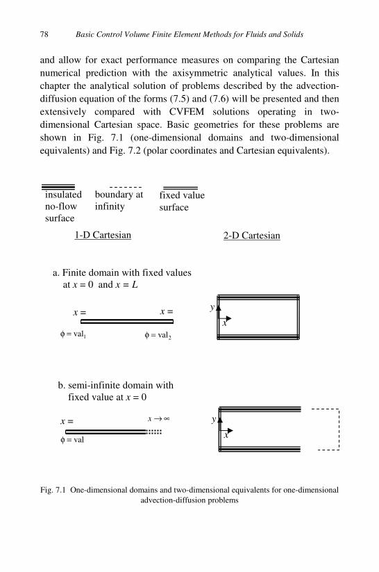
Basic Control Volume Finite Element Methods for Fluids and Solids
78
and allow for exact performance measures on comparing the Cartesian
numerical prediction with the axisymmetric analytical values. In this
chapter the analytical solution of problems described by the advection-
diffusion equation of the forms (7.5) and (7.6) will be presented and then
extensively compared with CVFEM solutions operating in two-
dimensional Cartesian space. Basic geometries for these problems are
shown in Fig. 7.1 (one-dimensional domains and two-dimensional
equivalents) and Fig. 7.2 (polar coordinates and Cartesian equivalents).
Fig. 7.1 One-dimensional domains and two-dimensional equivalents for one-dimensional
advection-diffusion problems
x =
0 val=φ
∞→x
x =
1val=φ2val=φ
x =
L
b. semi-infinite domain with
fixed value at x = 0
a. Finite domain with fixed values
at x = 0 and x = L
1-D Cartesian
Coordinates 2-D Cartesian
Coordinates
insulated
no-flow
surface
boundary at
infinity fixed value
surface
x
y
x
y
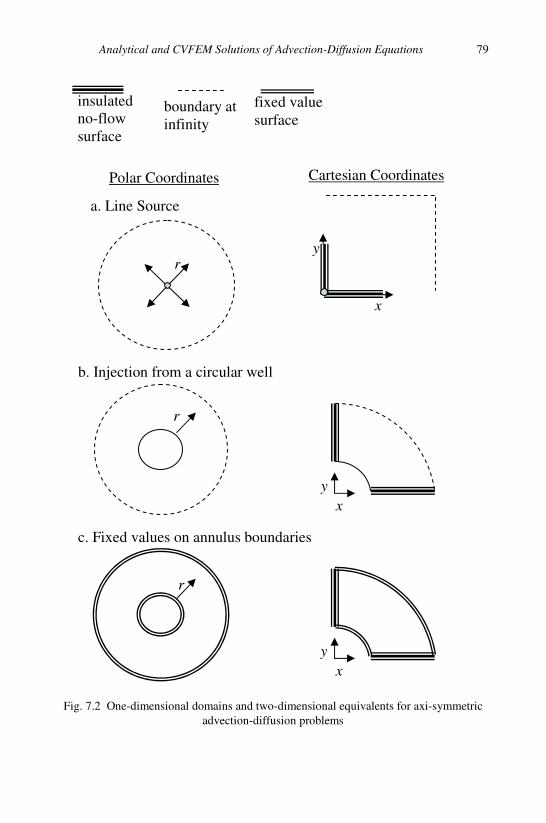
Analytical and CVFEM Solutions of Advection-Diffusion Equations
79
Fig. 7.2 One-dimensional domains and two-dimensional equivalents for axi-symmetric
advection-diffusion problems
insulated
no-flow
surface
boundary at
infinity
r
x
y
a. Line Source
b. Injection from a circular well
x
y
r
c. Fixed values on annulus boundaries
x
y
r
fixed value
surface
Polar Coordinates Cartesian Coordinates

Basic Control Volume Finite Element Methods for Fluids and Solids
80
7.3 One-Dimensional Steady State Diffusion in a Finite Domain
For this problem, (7.5) has the form
Lx,dx
d
dx
d≤≤=
φκ 00 (7.7)
in the fixed domain shown in Fig. 7.1a. If Dirichlet (fixed-value)
boundary conditions are imposed
10 φ=φ )( and 2φ=φ )L( (7.8)
and a constant diffusivity κ is assumed, the solution of (7.7) satisfying
(7.8) is
( ) 112 φ+φ−φ=φL
x (7.9)
If the diffusivity is given by )x( 1+α=κ where α is a constant the
solution of (7.7) satisfying (7.8) is
( ) 1121
1φ+
+
+φ−φ=φ
)L(ln
)x(ln (7.10)
The solutions of (7.9) and (7.10) are plotted for the case
0111 21 =φ=φ==α ,,L, in Fig. 7.3.
When the boundary conditions are given by
10 φ==φ )y,x( and 2φ==φ )y,Lx( (7.11a)
and
0=∂
φ∂
±= byy
(7.11b)
the solutions (7.9) and (7.10) can also be applied to the equivalent two-
dimensional problem (see right hand side of Fig. 7.1a) governed by
by,Lx,yyxx
≤≤≤≤=
∂
φ∂κ
∂
∂+
∂
φ∂κ
∂
∂000 (7.12)
where b is an arbitrary constant.

Analytical and CVFEM Solutions of Advection-Diffusion Equations
81
Fig. 7.3 Analytical (solid lines) and CVFEM (open squares) solutions of (7.12)
Fig. 7.4 Mesh for CVFEM solution of (7.12)
0
0.1
0.2
0.3
0.4
0.5
0.6
0.7
0.8
0.9
1
0 0.2 0.4 0.6 0.8 1
Position
Val
ue
constant=κ
x)α( +=κ 1

Basic Control Volume Finite Element Methods for Fluids and Solids
82
The CVFEM discretization for this problem, implemented on the mesh
shown in Fig. 7.4, is
∑=
+φ=φ+i
ij,ii
n
j
BSj,iiCi Ba]Ba[
1
(7.13)
The coefficients are generated from (5.27) and the boundary terms are set
such that (i) the upper (y = b= 0.25) and lower (y = 0) are insulated
( 00 == BC B,B ), (ii) the left hand boundary (x = 0) is the fixed value 1
( 1616 1010 == BC B,B ), and (iii) the right hand boundary (x = 1) is the
fixed value 0 ( 01016 == BC B,B ).The CVFEM solutions, obtained from
a point wise iteration of (7.13) are shown as the open squares superposed
on the analytical lines in Fig. 7.3. Although somewhat trivial the
agreement between the CVFEM and the analytical solution is excellent.
Note that this problem is a reasonable first test for the CVFEM, since
the grid in Fig. 7.4 is most defiantly not one-dimensional.
7.4 One-Dimensional Transient Diffusion in a Semi-Infinite Domain
For this problem (7.5) has the form
x,xxt
≤=
∂
φ∂κ
∂
∂−
∂
φ∂00 (7.14)
in the semi-infinite domain of Fig. 7.1b. Suitable boundary conditions
are
100 φ=>=φ )t,x( and 2φ=φ∞→x
lim (7.15)
with initial condition
200 φ==>φ )t,x( (7.16)
If the diffusivity is a constant then the solution of (7.14) - (7.16) is given
by
1122
φ+
κφ−φ=φ
t
xerf)( (7.17)

Analytical and CVFEM Solutions of Advection-Diffusion Equations
83
Fig. 7.5 Analytical (solid lines) and CVFEM (open squares) solutions of (7.22)
Fig. 7.6 Mesh for CVFEM solution of (7.22)
where
∫α
α−
πα=
0
22
de)z(erf (7.18)
0
0.1
0.2
0.3
0.4
0.5
0.6
0.7
0.8
0.9
1
0 2 4 6 8 10x- Distance
Val
ue
201 21 =κ=φ=φ ,,
t = 1.25t = 5
t = 2.5
Basic Control Volume Finite Element Methods for Fluids and Solids
84
is the error function (page 297 in Abramowitz and Stegun (1970)).
Calculation of the error function is built into many available commercial
computational packages. If a calculator is not available, however, it can
be estimated, to within an absolute error of 4105 −× , from the rational
approximation
078108000972230389278393
]1[
11
4321
444
33
221
.a,.a,.a,.a
xaxaxaxa)x(erf
====
++++−=
(7.19)
Example plots of the solution in (7.17), at three time steps, are shown as
solid lines in Fig. 7.5.
On imposing the boundary conditions
100 φ=>≤≤−=φ )t,byb,x( and 2φ=φ∞→x
lim (7.20a)
0
0
=∂
φ∂
∞<≤±= x,byy
(7.20b)
and the initial condition
2000 φ==≤≤>φ )t,by,x( (7.21)
The solution (7.17) is also applicable to the two-dimensional problem
by,x,yyxxt
≤≤∞≤≤=
∂
φ∂κ
∂
∂−
∂
φ∂κ
∂
∂−
∂
φ∂000 (7.22)
Where b is an arbitrary constant .The CVFEM discretization for this
problem, implemented on the mesh shown in Fig 7.6, is
i
i
j,ii B
n
j
iiSj,iiinewici BaatV)BV( +
φ−φ∆+φ=φ+ ∑
=1
(7.23)
In this mesh the long length (L = 20), chosen to mimic the far field
∞→x condition. The coefficients in (7.23) are generated from (5.27)
and the boundary terms are set so that (i) the upper (y = b= 4), lower
(y = 0) and right (far field) boundaries are insulated ( 00 == BC B,B )
and (ii) the left hand boundary (x = 0) is the fixed value
1( 1616 1010 == BC B,B ). The CVFEM solutions, obtained from the
explicit time marching solution of (7.23) (profile along y = 0) with time
Analytical and CVFEM Solutions of Advection-Diffusion Equations
85
step 31081257 −×=∆ .t are shown as the open squares superposed on the
analytical lines in Fig. 7.5. This solution is an excellent first test of the
performance of control volume methods on transient problems.
7.5 One-dimensional Transient Advection-Diffusion in a
Semi-Infinite Domain
Here all terms but the source term appears in the governing equation
x,xx
)v(xt
x ≤=
∂
φ∂κ
∂
∂−φ
∂
∂+
∂
φ∂00 (7.24)
Since the domain is one-dimensional (see Fig. 7.1b) the velocity v is a
constant scalar. If the diffusivity is also a constant (7.14) can be written
in the dimensionless form
x,xx
)(x
Pet
≤=
∂
φ∂
∂
∂−φ
∂
∂+
∂
φ∂00 (7.25)
where
κ
=Lv
Pe x (7.26)
is the Peclet number and L is a convenient length scale. A problem of
interest is the diffusion-advection of a step imposed and maintained at
the boundary x = 0. The appropriate boundary and initial conditions are
100 φ=>=φ )t,x( , 0=φ∞→x
lim (7.27)
000 ==>φ )t,x( (7.28)
The solution is
++
−φ=φ
t
tPexerfce
t
tPexerfc
xPe
222
2 (7.29)
where the complimentary error function )z(erf)z(erfc −= 1 (note
)z(erf)z(erfc +=− 1 ). Example plots of (7.29), for selected values of
the Peclet number, at time t = 5, are given by the solid lines in Fig. 7.7.

Basic Control Volume Finite Element Methods for Fluids and Solids
86
Fig. 7.7 Analytical (solid lines) and CVFEM (open squares) solutions of transient
advection-diffusion problem (7.24)
On imposing the boundary conditions
100 φ=>≤≤−=φ )t,byb,x( , 0=φ∞→x
lim (7.30a)
0
0
=∂
φ∂
∞<≤±= x,byy
(7.30b)
the initial condition
200 φ==≤≤−>φ )t,byb,x( (7.31)
0
0.1
0.2
0.3
0.4
0.5
0.6
0.7
0.8
0.9
1
0 5 10 15 20
x-position
val
ue Pe=1
Pe=0.5
Pe=2

Analytical and CVFEM Solutions of Advection-Diffusion Equations
87
and setting the velocities to 0== yx v,Pev the solution (7.29) is also
applicable to the two-dimensional problem
,yyxxy
)v(
x
)v(
t
yx 0=
∂
φ∂κ
∂
∂−
∂
φ∂κ
∂
∂−
∂
φ∂+
∂
φ∂+
∂
φ∂ (7.32)
where by,x ≤≤∞≤≤ 00 .The CVFEM discretization for this problem
is also given by (7.23). In setting up this equation the diffusive
contributions to the coefficients are calculated from (5.27) and the
advective contributions from (5.37). The CVFEM solution has been
implemented on the mesh shown in Fig 7.6, where the long length L = 20
is chosen to mimic the far field ∞→x condition. The settings of the
boundary terms are as in the previous problem, i.e., (i) the upper(y = b=
4), the lower(y = 0) and right (far field) boundaries are insulated
( 00 == BC B,B ) and (ii) the left hand boundary (x = 0) has the fixed
value 1 ( 1616 1010 == BC B,B ). The CVFEM solutions (profiles along y
= 0 for selected Peclet numbers at time t = 5) obtained from the explicit
time marching solution of (7.23) with time step 01250.t =∆ are shown as
the open squares superposed on the analytical lines in Fig. 7.7. At low
Peclet numbers (0.5 and 1) the agreement between the CVFEM and the
analytical solutions is excellent, indicating the ability of the CVFEM to
handle advection transport. As the Peclet number increases, however, we
notice a “smearing” in the CVFEM solution. This is due to the
“numerical dispersion” upwind feature noted in Chapter 5. The smearing
can be mitigated by using a finer mesh or implementing a higher order
upwind treatment, see Woodfield, Suzuki and Nakabe (2004).
7.6 Steady State Diffusion in an Annulus
7.6.1 Constant diffusivity
In cylindrical coordinates the governing equation, derived from (7.6), is
outin RrR,dr
dr
dr
d≤≤=
φ0 (7.33)

Basic Control Volume Finite Element Methods for Fluids and Solids
88
where inRr = and outRr = are the inner and out radii of the annulus
domain in Fig. 7.2c. The boundary conditions are
inin )Rr( φ==φ and outout )Rr( φ==φ (7.34)
The analytical solution is
)Rln()Rln(
)Rln()rln()(
inout
ininoutin
−
−φ−φ+φ=φ (7.35)
A particular solution, when 2101 ===φ=φ outinoutin R,R,, , is shown
by the dashed line in Fig. 7.8.
In two-dimensional Cartesian coordinates (considering the ¼ domain
on the right of Fig. 7.2c the problem statement is
outin RyxR,y,x,yx
≤+≤≥≥=∂
φ∂+
∂
φ∂ 22
2
2
2
2
000 (7.36)
with
122 =+φ=φ yxon,in , 222 =+φ=φ yxon,out (7.37)
00 ==∂
φ∂yon,
y, 00 ==
∂
φ∂xon,
x (7.38)
The CVFEM discretization for this problem, implemented on the mesh
shown in Fig. 7.9, is given by equation (7.13). The coefficients are
generated from (5.27). The boundary terms are set such that (i) for nodes
on the inner radius (r = 1) the fixed value 1 is imposed by setting 1616 1010 == BC B,B (ii) for nodes on the outer radius (r = 2) the fixed
value 0 is imposed on setting 1616 10210 ×== BC B,B (iii) all other
boundaries are insulated, i.e., 00 == BC B,B . The CVFEM solution is
obtained by a point wise iteration of (7.13). This two-dimensional
solution )y,x( iiφ can be compared to the one-dimensional analytical
axisymmetric solution (7.35) on setting
22iii yxrr +== .

Analytical and CVFEM Solutions of Advection-Diffusion Equations
89
Fig. 7.8 Steady state diffusion solution in annulus, lines axisymmetric solution, symbols
CVFEM Cartesian solution
a procedure that will be used thought out the treatment of annulus
problems. The CVFEM solution obtained in this way is shown as open
squares on Fig. 7.8. Note, essentially the only difference between the
CVFEM operation of this solution and the constant diffusion one-
dimensional solution discussed in §7.3 is the domain geometry and mesh,
i.e., the mesh in Fig. 7.4 vs. the mesh in Fig. 7.9.
0
0.1
0.2
0.3
0.4
0.5
0.6
0.7
0.8
0.9
1
1 1.2 1.4 1.6 1.8 2
Radial Position
Val
ue
α = 2α = 0

Basic Control Volume Finite Element Methods for Fluids and Solids
90
Fig. 7.9 Mesh for annulus problem
7.6.2 Variable diffusivity and source term
The previous problem can be extend by assuming a radial dependent
diffusivity and source
r1=κ ,
rQ α= , α = constant
In cylindrical coordinates the domain geometry is the left had side of
Fig. 7.2c and the governing equation is
outin RrR,dr
d≤≤=α+
φ0
2
2
(7.39)
With the boundary conditions
inin )Rr( φ==φ and outout )Rr( φ==φ (7.40)
When 2101 ===φ=φ outinoutin R,R,, the analytical solution is
0 0.5 1 1.5 20
0.2
0.4
0.6
0.8
1
1.2
1.4
1.6
1.8
2

Analytical and CVFEM Solutions of Advection-Diffusion Equations
91
α−+α−−α
−=φ 212 2
32r)(r (7.41)
This solution (with 0=α and 2 ) is plotted as the solid lines in Fig. 7.8.
In Cartesian coordinates (considering the ¼ domain on the right of
Fig. 7.2c) the governing equation is
21000 22 ≤+≤≥≥=+
∂
φ∂κ
∂
∂+
∂
φ∂κ
∂
∂yx,y,x,Q
yyxx (7.42)
with
11 22 =+=φ yxon, , 20 22 =+=φ yxon, (7.43a)
00 ==∂
φ∂yon,
y 00 ==
∂
φ∂xon,
x (7.43b)
and
2222
1
yxQ,
yx +
α=
+=κ (7.44)
This problem, testing the ability of the CVFEM to deal with spatial
variability in the diffusivity and source terms, is solved using the full
steady sate CVFEM discrete form in (7.3). In solving equations (7.42)-
(7.44) this discrete equation is implemented on the mesh shown in Fig.
7.9. The coefficients are calculated using (5.27)—taking care to account
for the variable conductivity. The boundary terms are identical to those
used in the previous problem in §7.6.1. The source terms in (7.3) are
calculated as
22
0
ii
iBC
yx
VQ,Qii
+
α== (7.45)
Where Vi is the volume of the control volume around node i. The
CVFEM solution is obtained by a point wise iteration of (7.3). The
CVFEM solution for the cases α = 0 and α = 2 are shown as open
squares in Fig. 7.8.
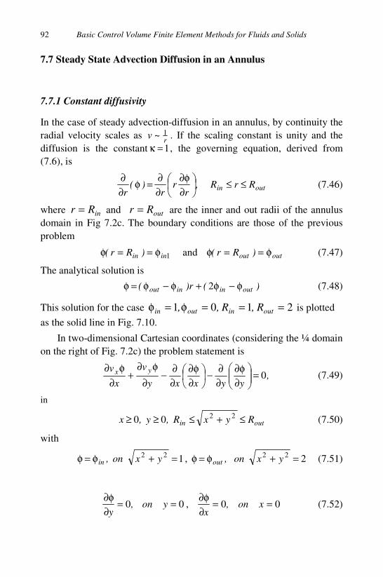
Basic Control Volume Finite Element Methods for Fluids and Solids
92
7.7 Steady State Advection Diffusion in an Annulus
7.7.1 Constant diffusivity
In the case of steady advection-diffusion in an annulus, by continuity the
radial velocity scales as r
~v 1 . If the scaling constant is unity and the
diffusion is the constant 1=κ , the governing equation, derived from
(7.6), is
outin RrR,r
rr
)(r
≤≤
∂
φ∂
∂
∂=φ
∂
∂ (7.46)
where inRr = and outRr = are the inner and out radii of the annulus
domain in Fig 7.2c. The boundary conditions are those of the previous
problem
1inin )Rr( φ==φ and outout )Rr( φ==φ (7.47)
The analytical solution is
)(r)( outininout φ−φ+φ−φ=φ 2 (7.48)
This solution for the case 2101 ===φ=φ outinoutin R,R,, is plotted
as the solid line in Fig. 7.10.
In two-dimensional Cartesian coordinates (considering the ¼ domain
on the right of Fig. 7.2c) the problem statement is
,yyxxy
v
x
v yx 0=
∂
φ∂
∂
∂−
∂
φ∂
∂
∂−
∂
φ∂+
∂
φ∂ (7.49)
in
outin RyxR,y,x ≤+≤≥≥ 2200 (7.50)
with
122 =+φ=φ yxon,in , 222 =+φ=φ yxon,out (7.51)
00 ==∂
φ∂yon,
y, 00 ==
∂
φ∂xon,
x (7.52)

Analytical and CVFEM Solutions of Advection-Diffusion Equations
93
Fig. 7.10 Advection-diffusion in an annulus (constant diffusivity). Solid line
axisymmetric analytical solution (7.48). Symbols CVFEM solution of (7.49)-(7.53)
and
)x/y(tan,
yx
)sin(v,
yx
)cos(v yx
1
2222
−=θ+
θ=
+
θ= (7.53)
This problem can be solved using the CVFEM discrete equation in
(7.13), the diffusive contributions to the coefficients calculated from
(5.27) and the advective contributions from (5.37). This solution can be
implemented on the mesh shown in Fig 7.9. For the example problem
in Fig. 7.10, the boundary terms are set such that (i) for nodes
on the inner radius (r = 1) the fixed value 1 is imposed by
setting 1616 1010 == BC B,B (ii) for nodes on the outer radius (r = 2) the
fixed value 0 is imposed on setting 1616 10210 ×== BC B,B (iii) all
0
0.1
0.2
0.3
0.4
0.5
0.6
0.7
0.8
0.9
1
1 1.5 2
Radial Position
Val
ue

Basic Control Volume Finite Element Methods for Fluids and Solids
94
other boundaries are insulated, i.e., 00 == BC B,B . The CVFEM
solution is obtained by a point wise iteration of (7.13). and compared
with the analytical solution in Fig. 7.9.
7.7.2 Variable diffusivity
In the previous problem if the diffusivity is given by
r
1=κ ,
a condition consistent with a dispersion dominated regime (see Hsieh
(1986)) the governing equation, in cylindrical coordinates becomes
outin RrR,rr
≤≤∂
φ∂=
∂
φ∂2
2
(7.54)
with boundary conditions identical to (7.47). The analytical solution,
when 2101 ===φ=φ outinoutin R,R,, , is
2
2
ee
eer
−
−=φ (7.55)
In Cartesian coordinates the governing equation is
,yyxxy
v
x
v yx 0=
∂
φ∂κ
∂
∂−
∂
φ∂κ
∂
∂−
∂
φ∂+
∂
φ∂ (7.56)
Subject to definitions and conditions in (7.50)-(7.53) along with the
additional definition
,
yx22
1
+=κ (7.57)
The setting of the variable diffusivity is the only change that needs to
be made to the CVFEM code used to solve the previous problem. The
comparison of this two-dimensional solution (open symbols) is compared
with the analytical solution of (7.55) in Fig. 7.11. The very slight under
prediction in the CVFEM solution is due to the relatively coarse mesh
used (see Fig. 7.8)). If a finer mesh is used the performance of the
CVFEM improves.
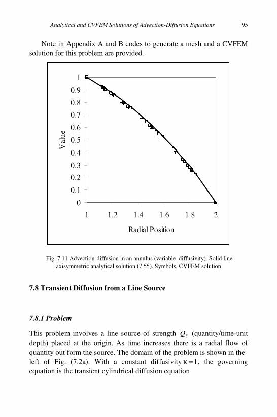
Analytical and CVFEM Solutions of Advection-Diffusion Equations
95
Note in Appendix A and B codes to generate a mesh and a CVFEM
solution for this problem are provided.
Fig. 7.11 Advection-diffusion in an annulus (variable diffusivity). Solid line
axisymmetric analytical solution (7.55). Symbols, CVFEM solution
7.8 Transient Diffusion from a Line Source
7.8.1 Problem
This problem involves a line source of strength ℓ
Q (quantity/time-unit
depth) placed at the origin. As time increases there is a radial flow of
quantity out form the source. The domain of the problem is shown in the
left of Fig. (7.2a). With a constant diffusivity 1=κ , the governing
equation is the transient cylindrical diffusion equation
0
0.1
0.2
0.3
0.4
0.5
0.6
0.7
0.8
0.9
1
1 1.2 1.4 1.6 1.8 2
Radial Position
Val
ue
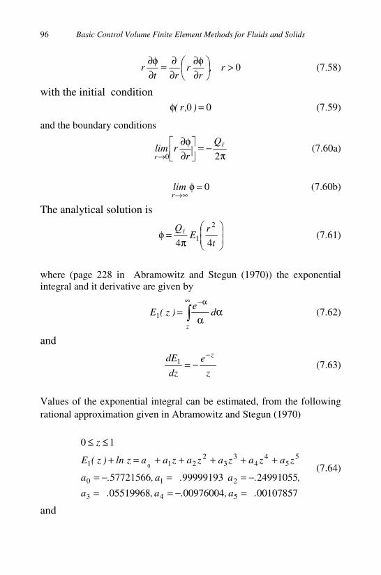
Basic Control Volume Finite Element Methods for Fluids and Solids
96
0>
∂
φ∂
∂
∂=
∂
φ∂r,
rr
rtr (7.58)
with the initial condition
00 =φ ),r( (7.59)
and the boundary conditions
π
−=
∂
φ∂
→ 20
ℓQ
rrlim
r (7.60a)
0=φ∞→r
lim (7.60b)
The analytical solution is
π=φ
t
rE
Q
44
2
1ℓ (7.61)
where (page 228 in Abramowitz and Stegun (1970)) the exponential
integral and it derivative are given by
αα
= ∫∞ α−
de
)z(E
z
1 (7.62)
and
z
e
dz
dE z−
−=1 (7.63)
Values of the exponential integral can be estimated, from the following
rational approximation given in Abramowitz and Stegun (1970)
001078570097600405519968
249910559999919357721566
10
543
210
55
44
33
2211 0
.a,.a,.a
,.a.a,.a
zazazazazaazln)z(E
z
=−==
−==−=
+++++=+
≤≤
(7.64)
and
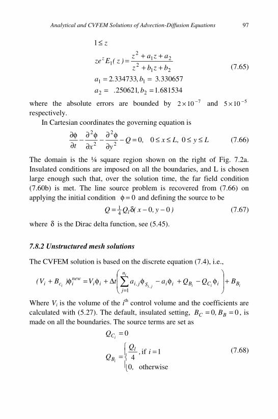
Analytical and CVFEM Solutions of Advection-Diffusion Equations
97
6815341250621
33065733347332
1
22
11
212
212
1
.b,.a
.b,.a
bzbz
azaz)z(Eze
z
z
==
==
++
++=
≤
(7.65)
where the absolute errors are bounded by 7102 −× and 5105 −×
respectively.
In Cartesian coordinates the governing equation is
Ly,Lx,Qyxt
≤≤≤≤=−∂
φ∂−
∂
φ∂−
∂
φ∂000
2
2
2
2
(7.66)
The domain is the ¼ square region shown on the right of Fig. 7.2a.
Insulated conditions are imposed on all the boundaries, and L is chosen
large enough such that, over the solution time, the far field condition
(7.60b) is met. The line source problem is recovered from (7.66) on
applying the initial condition 0=φ and defining the source to be
)y,x(QQ l 0041 −−δ= (7.67)
where δ is the Dirac delta function, see (5.45).
7.8.2 Unstructured mesh solutions
The CVFEM solution is based on the discrete equation (7.4), i.e.,
iii
i
j,ii BiCB
n
j
iiSj,iiinewici BQQaatV)BV( +
φ−+φ−φ∆+φ=φ+ ∑
=1
Where Vi is the volume of the ith control volume and the coefficients are
calculated with (5.27). The default, insulated setting, 00 == BC B,B , is
made on all the boundaries. The source terms are set as
=
=
=
otherwise0
1if4
0
,
i,Q
Q
Q
l
B
C
i
i
(7.68)
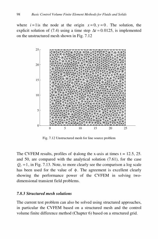
Basic Control Volume Finite Element Methods for Fluids and Solids
98
where 1=i is the node at the origin 00 == y,x . The solution, the
explicit solution of (7.4) using a time step .t 0=∆ 0125, is implemented
on the unstructured mesh shown in Fig. 7.12
Fig. 7.12 Unstructured mesh for line source problem
The CVFEM results, profiles of φ along the x-axis at times t = 12.5, 25.
and 50, are compared with the analytical solution (7.61), for the case
1=ℓ
Q , in Fig. 7.13. Note, to more clearly see the comparison a log scale
has been used for the value of φ . The agreement is excellent clearly
showing the performance power of the CVFEM in solving two-
dimensional transient field problems.
7.8.3 Structured mesh solutions
The current test problem can also be solved using structured approaches,
in particular the CVFEM based on a structured mesh and the control
volume finite difference method (Chapter 6) based on a structured grid.
0 5 10 15 20 250
5
10
15
20
25

Analytical and CVFEM Solutions of Advection-Diffusion Equations
99
Fig. 7.13 Results for line source problem when 1=
ℓQ . Solid line analytical solution
(7.61), open symbols CVFEM solution implemented on mesh in Fig. 7.12
CVFEM on a structured grid: The CVFEM solution above can
immediately be implemented on the structured mesh shown in Fig. 7.14.
The results, profile of φ along the x-axis at time t = 50, are compared
with the analytical solution (7.61), for the case 1=ℓ
Q , in Fig. 7.15.
CVFDM solution: Taking guidance from the work in Chapter 6, the
control volume finite difference method (CVFDM) applied to the
governing equation (7.66) has the discrete explicit transient form
0.001
0.01
0.1
1
0 5 10 15 20
Radial Distance
log
val
ue
t =25 t =12.5
t =50

Basic Control Volume Finite Element Methods for Fluids and Solids
100
Fig. 7.14 Structured CVFEM mesh
[ ]ijj,iijijijij
Qaaaaat
yxyx
j,ipj,iej,isj,iwj,in
j,iijijnew
j,iijij
+φ−φ+φ+φ+φ∆+
φ∆∆=φ∆∆
+−−+ 1111
(7.69)
An appropriate control volume grid is given in Fig 7.16. Working on this
grid the coefficients in (7.69) are calculated using (6.16). The appropriate
coefficients in volumes adjacent to the insulated boundary are set to zero.
The source term ijQ is set using the second part of (7.68). With the
coefficients and source terms calculated (7.79) can be solved by explicit
time marching using a step of 0250.t =∆ . The results (profile along the
lowest layer of node points in Fig. 7.15)) obtained in this manner are
compared with the analytical solution (7.61) in Fig. 7.15.
7.9 The Recharge Well Problem
A vertical recharge well of radius wrr = issues a flow Q (volume/time)
into a horizontal uniformly thick ( b ) porous (porosity ε ) aquifer. At time
t = 0 a concentration of 0φ is introduce and held fixed in the well. This
concentration is transported into the aquifer by both advection and
hydraulic dispersion. In the radial direction the flow velocity is
0 5 10 15 20 250
5
10
15
20
25
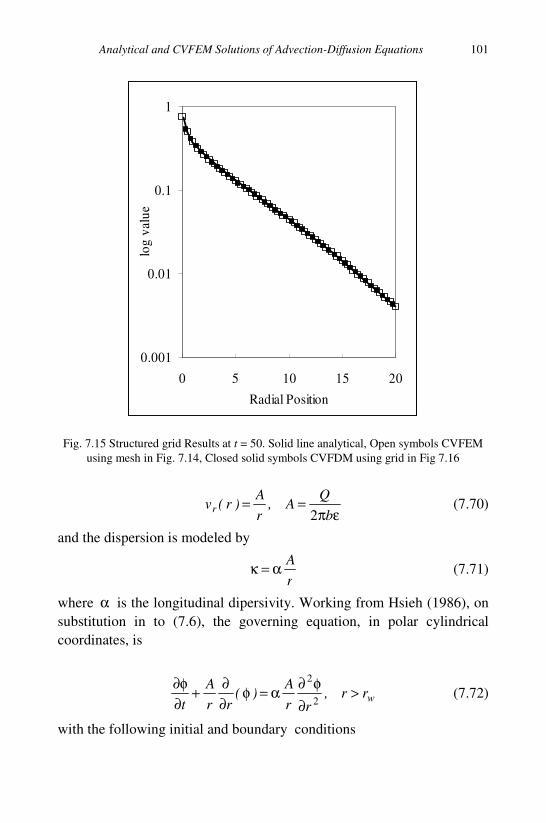
Analytical and CVFEM Solutions of Advection-Diffusion Equations
101
Fig. 7.15 Structured grid Results at t = 50. Solid line analytical, Open symbols CVFEM
using mesh in Fig. 7.14, Closed solid symbols CVFDM using grid in Fig 7.16
επ
==b
QA,
r
A)r(vr
2 (7.70)
and the dispersion is modeled by
r
Aα=κ (7.71)
where α is the longitudinal dipersivity. Working from Hsieh (1986), on
substitution in to (7.6), the governing equation, in polar cylindrical
coordinates, is
wrr,rr
A)(
rr
A
t>
∂
φ∂α=φ
∂
∂+
∂
φ∂2
2
(7.72)
with the following initial and boundary conditions
0.001
0.01
0.1
1
0 5 10 15 20
Radial Position
log
val
ue

Basic Control Volume Finite Element Methods for Fluids and Solids
102
Fig. 7.16 Control volume finite difference grid
000000 0 =>∞→φφ=>φ=>φ )t,r(,)t,r(,),r( w (7.73)
The analytical solution can be obtained via a Lapalce transform. This
solution is too detailed to presents here. Fortunately, however, Hsieh
(1986) has tabulated numerical values of the solution for various choices
of the problem parameters; a selection of these tabulations is reproduced
in Table 7.1.
In two-dimensional Cartesian coordinates the governing equation is
given by (7.32)
w
yx ryx,yyxxy
)v(
x
)v(
t≥+=
∂
φ∂κ
∂
∂−
∂
φ∂κ
∂
∂−
∂
φ∂+
∂
φ∂+
∂
φ∂ 220
The domain (a ¼ section) and an unstructured mesh for this problem
when rw = 10 is shown in Fig. 7.17. In this domain the initial condition is
0=φ )y,x( , all the boundaries are set as no-flow boundaries apart from
the curved well surface where
0 5 10 15 20 250
5
10
15
20
25
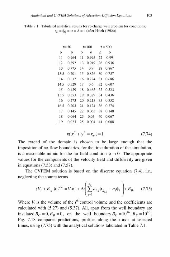
Analytical and CVFEM Solutions of Advection-Diffusion Equations
103
Table 7.1 Tabulated analytical results for re-charge well problem for conditions,
10 ==α=φ= Arw (after Hsieh (1986))
122 ==+φ )ryx( w (7.74)
The extend of the domain is chosen to be large enough that the
imposition of no-flow boundaries, for the time duration of the simulation,
is a reasonable mimic for the far field condition 0→φ . The appropriate
values for the components of the velocity field and diffusivity are given
in equations (7.53) and (7.57).
The CVFEM solution is based on the discrete equation (7.4), i.e.,
neglecting the source terms
i
i
j,ii B
n
j
iiSj,iiinewici BaatV)BV( +
φ−φ∆+φ=φ+ ∑
=1
(7.75)
Where Vi is the volume of the ith control volume and the coefficients are
calculated with (5.27) and (5.37). All, apart from the well boundary are
insulated 00 == BC B,B , on the well boundary 1616 1010 == BC B,B .
Fig. 7.18 compares predictions, profiles along the x-axis at selected
times, using (7.75) with the analytical solutions tabulated in Table 7.1.
τ= 50 τ=100 τ = 500
ρ φ ρ φ ρ φ
11 0.964 11 0.993 22 0.99
12 0.892 13 0.949 26 0.936
13 0.775 14 0.9 28 0.867
13.5 0.701 15 0.826 30 0.757
14 0.617 16 0.724 31 0.686
14.5 0.529 17 0.6 32 0.607
15 0.439 18 0.463 33 0.523
15.5 0.353 19 0.329 34 0.436
16 0.273 20 0.213 35 0.352
16.5 0.203 21 0.124 36 0.274
17 0.145 22 0.065 38 0.148
18 0.064 23 0.03 40 0.067
19 0.023 25 0.004 44 0.008
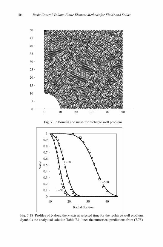
Basic Control Volume Finite Element Methods for Fluids and Solids
104
Fig. 7.17 Domain and mesh for recharge well problem
Fig. 7.18 Profiles of φ along the x-axis at selected time for the recharge well problem.
Symbols the analytical solution Table 7.1, lines the numerical predictions from (7.75)
0 10 20 30 40 500
5
10
15
20
25
30
35
40
45
50
0
0.1
0.2
0.3
0.4
0.5
0.6
0.7
0.8
0.9
1
10 20 30 40
Radial Position
Val
ue
t =50
t =100
t =500

Analytical and CVFEM Solutions of Advection-Diffusion Equations
105
The comparison in Fig. 7.18 clearly shows the ability of the CVFEM to
deal with a general transient two-dimensional advection –diffusion
problem. The slight disagreement is attributed to artificial dispersion
(numerical dissipation) which is a feature of the grid size.
106
Chapter 8
A Plane Stress CVFEM Solution
The control volume finite element method (CVFEM) is applied to the
solution of a plane stress problem.
8.1 Introduction
The task in this chapter is outline how the CVFEM can be applied in the
solution of a linear elastic problem. The problem chosen is the stress
concentration due to a hole in an infinite plate subjected to a uniaxial
load. The problem will be cast and solved as a plane stress problem.
Recall however, by the result in §2.2.6, a plane stress solution can be
converted to a plane strain solution through an appropriate re-definition
of the Young’s modulus, Poisson’s ratio, and thermal expansion
coefficient.
8.2 The Stress Concentration Problem
The problem domain is shown in Figure 8.1. This domain consists of a
¼ of finite plate of dimensions 200×200 mm with a center hole of radius
mma 10= . On the right side of the domain a uniaxial (x-direction) stress 2
0 1 mm/N=σ is applied. The top side of the domain and the hole is
unconstrained. The left boundary is constrained in the x –direction and
the bottom boundary in the y-direction. Following Kikuchi (1986), The
Young’s modulus is 251012 mm/N.E ×= , the Poisson’s ratio is
,.290=ν and the plate has a nominal thickness t = 10mm. There is a
classical solution for this problem in cylindrical polar coordinates due to
Timoshenko and Goodier (see page 231 in Kikuchi (1986)).

A Plane Stress CVFEM Solution
107
Fig. 8.1 Domain for stress concentration problem
This solution can be used to analytically determine the stress
concentration 0σσ=σ /xxc along the y-axis
ay,x,y
a
y
ac ≥=
++
+=σ 0311
2
142
(8.1)
8.3 CVFEM Displacement Solution
In terms of the displacements )u,u( yx the Cartesian statement of this
problem, derived from (2.29) can be written as
0=∂
∂κ+
∂
∂νκ+
∂
∂κ+
∂
∂κ∫
S
y
y
xyx
y
xxyx
xyxx
xx dSnx
un
y
un
y
un
x
u (8.2a)
0 20 40 60 80 1000
10
20
30
40
50
60
70
80
90
100
0 20 40 60 80 1000
10
20
30
40
50
60
70
80
90
100

Basic Control Volume Finite Element Methods for Fluids and Solids
108
0=∂
∂νκ+
∂
∂κ+
∂
∂κ+
∂
∂κ∫
S
yx
yyxx
xyyy
yyxy
xy dSnx
un
y
un
y
un
x
u (8.2b)
Fig. 8.2 Arrangement of control volumes and elements
where
)](/[E),/(E xyyyxx ν+=κν−=κ=κ 121 2 (8.3)
i
j = 4
k = Si,4
j = 1 or 5
k = Si,1 or Si,5
j = 2
k = Si,2
j = 3
k = Si,3
43 =≡ j
32 =≡ ji≡1
i
j = 4
k = Si,4
j = 1 or 5
k = Si,1 or Si,5
j = 2
k = Si,2
j = 3
k = Si,3
43 =≡ j
32 =≡ ji≡1
f1
f2
i
j = 4
k = Si,4
j = 1 or 5
k = Si,1 or Si,5
j = 2
k = Si,2
j = 3
k = Si,3
43 =≡ j
32 =≡ ji≡1
i
j = 4
k = Si,4
j = 1 or 5
k = Si,1 or Si,5
j = 2
k = Si,2
j = 3
k = Si,3
43 =≡ j
32 =≡ ji≡1
f1
f2
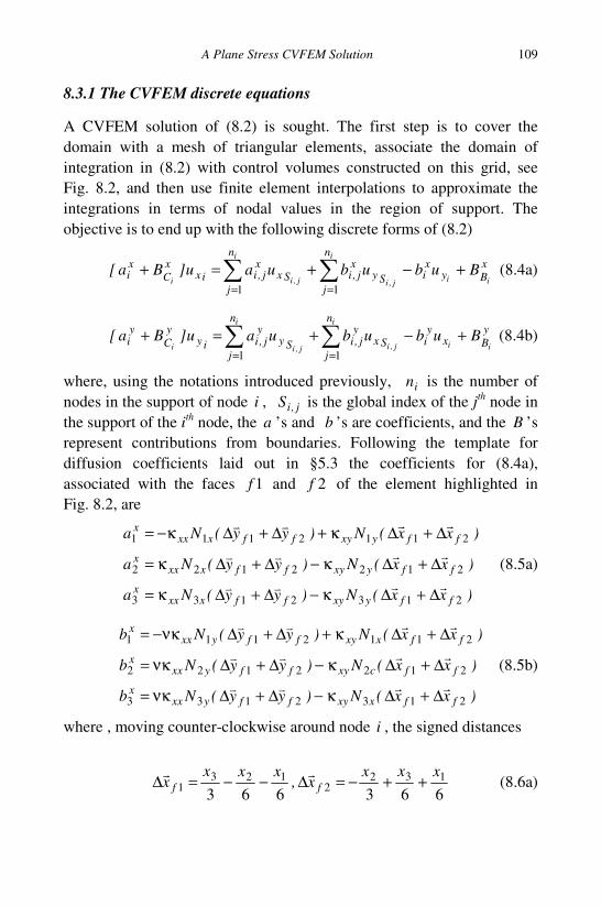
A Plane Stress CVFEM Solution
109
8.3.1 The CVFEM discrete equations
A CVFEM solution of (8.2) is sought. The first step is to cover the
domain with a mesh of triangular elements, associate the domain of
integration in (8.2) with control volumes constructed on this grid, see
Fig. 8.2, and then use finite element interpolations to approximate the
integrations in terms of nodal values in the region of support. The
objective is to end up with the following discrete forms of (8.2)
x
Byxi
n
jSy
xj,i
n
jSx
xj,iix
x
C
xi
ii
i
j,i
i
j,iiBububuau]Ba[ +−+=+ ∑∑
== 11
(8.4a)
y
Bxy
i
n
jSx
yj,i
n
jSy
yj,iiy
y
C
yi
ii
i
j,i
i
j,iiBububuau]Ba[ +−+=+ ∑∑
== 11
(8.4b)
where, using the notations introduced previously, in is the number of
nodes in the support of node i , j,iS is the global index of the jth node in
the support of the ith node, the a ’s and b ’s are coefficients, and the B ’s
represent contributions from boundaries. Following the template for
diffusion coefficients laid out in §5.3 the coefficients for (8.4a),
associated with the faces 1f and 2f of the element highlighted in
Fig. 8.2, are
)xx(N)yy(Na
)xx(N)yy(Na
)xx(N)yy(Na
ffyxyffxxxx
ffyxyffxxxx
ffyxyffxxxx
2132133
2122122
2112111
∆+∆κ−∆+∆κ=
∆+∆κ−∆+∆κ=
∆+∆κ+∆+∆κ−=
(8.5a)
)xx(N)yy(Nb
)xx(N)yy(Nb
)xx(N)yy(Nb
ffxxyffyxxx
ffcxyffyxxx
ffxxyffyxxx
2132133
2122122
2112111
∆+∆κ−∆+∆νκ=
∆+∆κ−∆+∆νκ=
∆+∆κ+∆+∆νκ−=
(8.5b)
where , moving counter-clockwise around node i , the signed distances
663663
1322
1231
xxxx,
xxxx ff ++−=∆−−=∆
(8.6a)
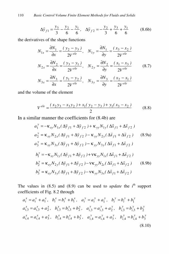
Basic Control Volume Finite Element Methods for Fluids and Solids
110
663663
1322
1231
yyyy,
yyyy ff ++−=∆−−=∆
(8.6b)
the derivatives of the shape functions
eleyelex
eleyelex
eleyelex
V
)xx(
y
NN,
V
)yy(
x
NN
V
)xx(
y
NN,
V
)yy(
x
NN
V
)xx(
y
NN,
V
)yy(
x
NN
22
22
22
1233
2133
3122
1322
2311
3211
−=
∂
∂=
−=
∂
∂=
−=
∂
∂=
−=
∂
∂=
−=
∂
∂=
−=
∂
∂=
(8.7)
and the volume of the element
2
2313212332 )xx(y)yy(x)yxyx(V
ele −+−+−= (8.8)
In a similar manner the coefficients for (8.4b) are
)xx(N)yy(Na
)xx(N)yy(Na
)xx(N)yy(Na
ffyyyffxxyy
ffyyyffxxyy
ffyyyffxxyy
2132133
2122122
2112111
∆+∆κ−∆+∆κ=
∆+∆κ−∆+∆κ=
∆+∆κ+∆+∆κ−=
(8.9a)
)xx(N)yy(Nb
)xx(N)yy(Nb
)xx(N)yy(Nb
ffxyyffyxyy
ffcyyffyxyy
ffxyyffyxyy
2132133
2122122
2112111
∆+∆νκ−∆+∆κ=
∆+∆νκ−∆+∆κ=
∆+∆νκ+∆+∆κ−=
(8.9b)
The values in (8.5) and (8.9) can be used to update the ith support
coefficients of Fig. 8.2 through
yy,i
y,i
yy,i
y,i
xx,i
x,i
xx,i
x,i
yy,i
y,i
yy,i
y,i
xx,i
x,i
xx,i
x,i
yyi
yi
yyi
yi
xxi
xi
xxi
xi
bbb,aaa,bbb,aaa
bbb,aaa,bbb,aaa
bbb,aaa,bbb,aaa
344344344344
233233233233
1111
+=+=+=+=
+=+=+=+=
+=+=+=+=
(8.10)

A Plane Stress CVFEM Solution
111
In this way, by calling at each element in the support of node i , the
coefficients in (8.4) can be calculated.
8.3.2 Boundary conditions
The coefficients derived above account for the tractions acting on the
internal faces of a given control volume. To complete the discrete
equations (8.4) it is necessary to add in the applied tractions on the right
hand vertical boundary ( mmx 100= ). Fig. 8.3 shows a typical control
volume on this boundary
Fig. 8.3 Node and control volume on traction boundary
With reference to this figure the traction boundary is imposed by
setting at each node j on this boundary
00 ===σ∆= yC
yB
xCj
xB BBB,B (8.11)
where the lengths j∆ are calculated from
12
2
2
2
1
11
12
−≤≤
−
−
−
=∆
−
−+ B
BnBn
BB
BB
j nj,
/)yy(
/)yy(
/)yy(
BB
jj (8.12)
σ0j ∆σ0j ∆

Basic Control Volume Finite Element Methods for Fluids and Solids
112
Bn is the number of nodes on the boundary segment where the traction is
applied , and jB is the global node number of the jth node on the
boundary.
On each node on the left hand vertical boundary 0=x the zero x-
displacement condition is applied by setting
01016 ==== yC
yB
xB
xC BBB,B (8.13)
On each node the lower horizontal boundary 0=y the zero y-
displacement condition is applied by setting
01016 ==== xC
yB
xB
yC BBB,B (8.14)
On all other boundaries no constraints are imposed, i.e., at each node
0==== yC
xC
yB
xB BBBB (8.15)
8.3.3 Solution
The work above fully specifies the coefficients in (8.4). Solution, the
nodal displacement field )u,u( yx can be readily achieved by a point
iteration. Figure 8.4 graphically illustrates the displacement solution by
showing, in exaggerated form, the deformed shape of the plate after
application of the uniaxial stress; this figure also shows the grid used in
the calculation. When a larger hole ( mma 40= instead of mma 10= ) is
used the deformations are much more pronounced, Fig. 8.5. Note with
the larger hole the top free surface undergoes a rotation not seen with the
smaller hole. This would suggest that with the larger hole the comparison
with the analytical stress solution (8.1), requiring an infinite plate, may
not be valid. This will be confirmed in the next section where it is shown
how to calculate the stress field associated with the solution of (8.4)
8.4 The Stress Solution
In order to compare the solution from (8.4) with the analytical solution in
(8.1) it is necessary to calculate the stress filed associated with the
displacement fields solved by (8.4).
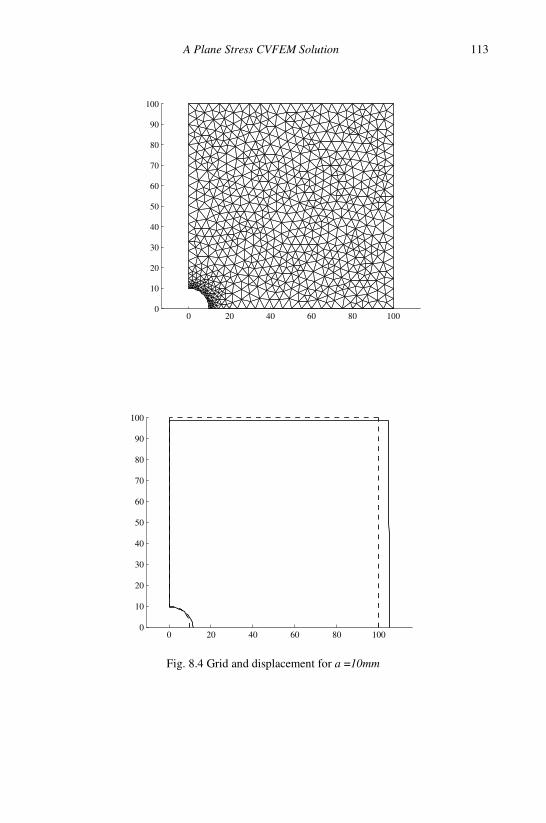
A Plane Stress CVFEM Solution
113
Fig. 8.4 Grid and displacement for a =10mm
0 20 40 60 80 1000
10
20
30
40
50
60
70
80
90
100
0 20 40 60 80 1000
10
20
30
40
50
60
70
80
90
100

Basic Control Volume Finite Element Methods for Fluids and Solids
114
Fig. 8.5 Grid and displacement for a = 40mm
0 20 40 60 80 1000
10
20
30
40
50
60
70
80
90
100
0 20 40 60 80 1000
10
20
30
40
50
60
70
80
90
100
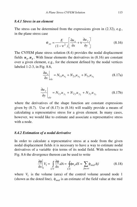
A Plane Stress CVFEM Solution
115
8.4.1 Stress in an element
The stress can be determined from the expressions given in (2.32), e.g.,
in the plane stress case
∂
∂ν+
∂
∂
ν−=σ
y
u
x
u
)(
E yxxx 21
(8.16)
The CVFEM plane stress solution (8.4) provides the nodal displacement
fields yx uu , . With linear elements the derivatives in (8.16) are constant
over a given element, e.g., for the element defined by the nodal vertices
labeled 1-2-3, in Fig. 8.6,
321 321 xxxxxx
ele
x uNuNuNx
u++=
∂
∂ (8.17a)
321 321 yyyyyy
ele
yuNuNuN
y
u++=
∂
∂ (8.17b)
where the derivatives of the shape function are constant expressions
given by (8.7). Use of (8.17) in (8.16) will readily provide a means of
calculating a representative stress for a given element. In many cases,
however, we would like to estimate and associate a representative stress
with a node.
8.4.2 Estimation of a nodal derivative
In order to calculate a representative stress at a node from the given
nodal displacement fields it is necessary to have a way to estimate nodal
derivatives of a variable φ in terms of its nodal field. With reference to
Fig. 8.6 the divergence thereon can be used to write
∫ ∑∫ ∆φ≈φ=∂
φ∂=
∂
φ∂
CV faces
mid
CS
x ydSndAx
Vx
11
(8.18)
where 1V is the volume (area) of the control volume around node 1
(shown as the doted line), midφ is an estimate of the field value at the mid

Basic Control Volume Finite Element Methods for Fluids and Solids
116
Fig. 8.6 A control volume and element arrangement
point of a face on the control volume (calculated in terms of the element
nodal values via the linear shape functions defined in (3.9)), and y
∆ is
the change in y moving along a given face in a counter-clockwise
direction. Equation (8.18) immediately implies that nodal derivatives can
be calculated as
,V/xy
,V/yx
faces
mid
faces
mid 1
1
11
∑∑ ∆φ−=∂
φ∂∆φ=
∂
φ∂
(8.19)
Note as written (8.19) is valid for internal nodes. For boundary nodes the
control volume surface includes both faces and the parts of the element
sides that coincide with the boundary. In this case (8.19) may require
additional terms to account for contributions from the element side
surfaces. For example, consider the section of domain boundary (heavy
lines), shown in Fig. 8.7. When calculating a derivative associated with
the corner node 1, in addition to the two mid face (a and b) terms in
(8.19), the additional terms
12
3
12
3

A Plane Stress CVFEM Solution
117
Fig. 8.7 Single element support on a domain boundary
−
φ+
φ=
−
φ+
φ=
2244
32
2244
31
3131
1221
yyE
yyE
(8.20)
evaluated at the mid-points of the element sides (c and d) need to be
included in the calculation of 1)x/( ∂φ∂ . Equation (8.20) can also be
written in terms the derivatives of the shape functions, i.e.,
φ+
φ−=
φ+
φ−=
xx
xx
NNE
NNE
23
21
32
31
44
32
88
31
(8.21)
1
2
3
a
b
c
d1
2
3
a
b
c
d

Basic Control Volume Finite Element Methods for Fluids and Solids
118
Note, for the elements in the support of an internal node, as we move
counter-clockwise from element e1 to element e2
22
13
23
12
eeex
ex ,NN φ−=φ−= (8.22)
Hence on completing the circuit around node 1 the extra terms in (8.20)
or (8.21) will cancel out and the derivatives at the internal node 1 can be
calculated directly by (8.19).
An alternative form of (8.19) can be obtained by expanding. Consider
the element with vertices labeled 1, 2 and 3 in the support of node 1 in
Fig. 8.6. By (8.19) the contributions of the two control volume faces
( 21 f,f ) in this element to the nodal derivative 1)x/( ∂φ∂ can be
expanded as
+−
φ+
φ+
φ+
+−−
φ+
φ+
φ=∆φ+∆φ
63612
5
12
2
12
5
36612
2
12
5
12
5
321321
3213212211
yyy
yyyyy ffff
(8.23)
On multiplying out the right hand side, gathering terms and using the
definitions of the shape function derivatives
213
213
3322112211
EEx
V
EE)NNN(V
yy
ele
ele
xxx
ele
ffff
−−∂
φ∂=
−−φ+φ+φ=∆φ+∆φ
(8.24)
On substitution into (8.19), at internal nodes the extra terms 21 E,E in
(8.24) cancel by (8.22) and at boundary nodes they cancel by (8.21).
Hence, the derivatives at a node can be determined in terms of the area
averaged element derivatives, i.e.,
1
support
11
support
1
33
V
y
V
y,
V
x
V
x
ele
ele
ele
ele
∑∑∂
φ∂
=∂
φ∂∂
φ∂
=∂
φ∂ (8.25)
an equivalent easier to use form of (8.19).
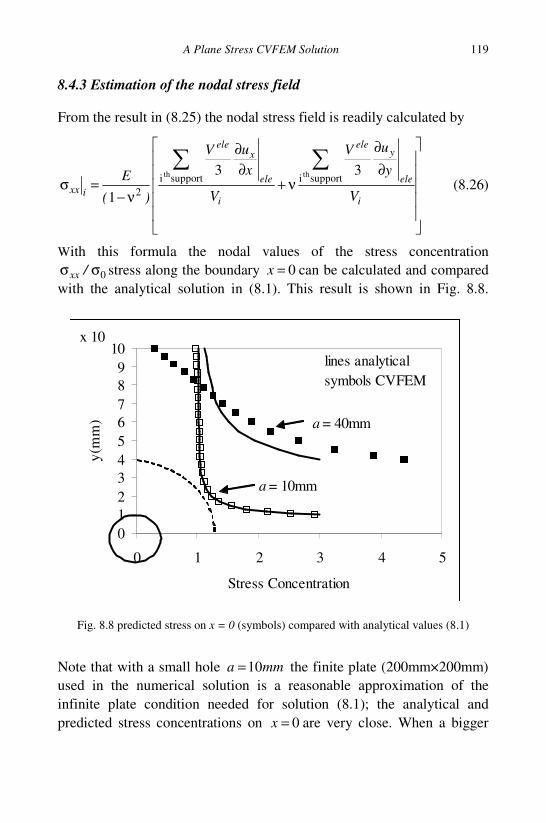
A Plane Stress CVFEM Solution
119
8.4.3 Estimation of the nodal stress field
From the result in (8.25) the nodal stress field is readily calculated by
∂
∂
ν+∂
∂
ν−=σ
∑∑
i
ele
yele
i
ele
xele
ixxV
y
uV
V
x
uV
)(
E supportisupporti
2
thth 33
1 (8.26)
With this formula the nodal values of the stress concentration
0σσ /xx stress along the boundary 0=x can be calculated and compared
with the analytical solution in (8.1). This result is shown in Fig. 8.8.
Fig. 8.8 predicted stress on x = 0 (symbols) compared with analytical values (8.1)
Note that with a small hole mma 10= the finite plate (200mm×200mm)
used in the numerical solution is a reasonable approximation of the
infinite plate condition needed for solution (8.1); the analytical and
predicted stress concentrations on 0=x are very close. When a bigger
0
1
2
3
4
5
6
7
8
9
10
0 1 2 3 4 5
Stress Concentration
y(m
m)
x 10
lines analytical
symbols CVFEM
a = 40mm
a = 10mm

Basic Control Volume Finite Element Methods for Fluids and Solids
120
hole is used however ( )mma 40= the validity of the numerical solution
to match the analytical conditions clearly breaks down.
8.5 Summary
Although a relatively simple plane stress problem has been solved this
chapter contains all of the ingredients required for a reader to develop a
CVFEM solution for any plane-stress or plane strain linear elastic
problem.

121
Chapter 9
CVFEM Stream Function-Vorticity Solution
for a Lid Driven Cavity Flow
A Control Volume Finite Element Solution for the stream-function—
vorticity formulation of lid driven cavity flow is presented.
9.1 Introduction
A classic test problem in computational fluid mechanics is a lid driven
cavity flow. In this two dimensional problem, the flow in a square
conduit is induced by sliding the upper surface (the lid) at a constant x-
velocityU , see Figure 9.1
Fig. 9.1 Lid driven cavity flow with streamline indicating flow
0 0.2 0.4 0.6 0.8 10
0.1
0.2
0.3
0.4
0.5
0.6
0.7
0.8
0.9
1U
0 0.2 0.4 0.6 0.8 10
0.1
0.2
0.3
0.4
0.5
0.6
0.7
0.8
0.9
1U
Basic Control Volume Finite Element Methods for Fluids and Solids
122
The nature of the flow in the cavity is controlled by a Reynolds Number
defined as
ν
=UL
Re (9.1)
Where L is the dimension of the cavity and ν is the kinematic viscosity.
Although no analytical solution exists there is an accepted benchmark by
Ghia, Ghia and Shin (1982) who use a multi-grid solution of the Navier-
Stokes equations in terms of primitive variables (velocity and pressure).
In this work a CVFEM stream-function-vorticity solution will be sough.
9.2 The Governing Equations
In terms of the stream function Ψ and vorticity ω the governing
equations, in integral form, are given by (2.50) and (2.51),
0=⋅ω∇ν−⋅ω∫ dS
S
nnv (9.2)
∫ ∫ ⋅ψ∇=ω−
A S
dSdA n (9.3)
In terms of the velocity field, v , the vorticity and stream function are
defined by
y
v
x
vxy
∂
∂−
∂
∂=ω (9.4)
x
v,y
v yx∂
Ψ∂−=
∂
Ψ∂= (9.5)
The boundary condition on (9.3) is
0=Ψ on all solid boundaries (9.6)
There is not an explicit boundary condition for the vorticity equation
(9.2). As will be detailed below, in setting up the numerical solution of
(9.2) and (9.3) a boundary condition for the solution of the discrete form

CVFEM Stream Function-Vorticity Solution for a Lid Driven Cavity Flow
123
of (9.2) is established by using the discrete form of (9.3) at boundary
nodes coupled with the known velocity conditions, i.e.,
boundaries allon 0
boundariesother allon 0 lid,on
=
==
y
xx
u
uUu (9.7)
9.3 The CVFEM Discretization of the Stream Function Equation
In keeping with rest of this monograph the development of the discreet
equations is based on linear triangular elements. The key components of
this discretization, the support, control volume, the element, and the
control volume faces (f1, f2) in an element are illustrated in Fig. 9.2. It is
convenient to first consider the discretization of the stream function
equation (9.3). The form of this equation can be identified as steady state
diffusion with a volume source. As such, developing the CVFE
discretization can be directly based on the calculations presented in §5.3
and § 5.5. The general form for the discrete equation, for node i in the
support shown in Fig. 9.2, is
∑=
ΨΨΨΨΨΨ ++Ψ=Ψ++i
iij,iii
n
j
BBSj,iiCCi BQa]BQa[
1
(9.8)
where the a ’s are the coefficients, the index )j,i( indicates the thj
node ( in,..,j 21= ) in the support of node i , the index j,iS provides the
global node number ( n,..,,i 321= ) of the thj node in the support, the B ’s
account for boundary conditions, and the Q ‘s for source terms.
9.3.1 Diffusion contributions
Following the presentation in §5.3 the contribution to the coefficients
a in (9.8), obtained from consideration of the diffusion flux across the
control volume faces (f1, f2) for the particular element in Fig. 9.2, are
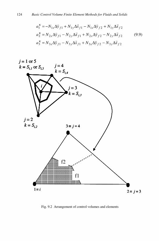
Basic Control Volume Finite Element Methods for Fluids and Solids
124
232313133
222212122
212111111
fyfxfyfx
fyfxfyfx
fyfxfyfx
xNyNxNyNa
xNyNxNyNa
xNyNxNyNa
∆−∆+∆−∆=
∆−∆+∆−∆=
∆+∆−∆+∆−=
κ
κ
κ
(9.9)
Fig. 9.2 Arrangement of control volumes and elements
i
j = 4
k = Si,4
j = 1 or 5
k = Si,1 or Si,5
j = 2
k = Si,2
j = 3
k = Si,3
43 =≡ j
32 =≡ ji≡1
i
j = 4
k = Si,4
j = 1 or 5
k = Si,1 or Si,5
j = 2
k = Si,2
j = 3
k = Si,3
43 =≡ j
32 =≡ ji≡1
f1
f2
i
j = 4
k = Si,4
j = 1 or 5
k = Si,1 or Si,5
j = 2
k = Si,2
j = 3
k = Si,3
43 =≡ j
32 =≡ ji≡1
i
j = 4
k = Si,4
j = 1 or 5
k = Si,1 or Si,5
j = 2
k = Si,2
j = 3
k = Si,3
43 =≡ j
32 =≡ ji≡1
f1
f2

CVFEM Stream Function-Vorticity Solution for a Lid Driven Cavity Flow
125
These values can be used to update the ith support coefficients through
κΨΨ
κΨΨ
κΨΨ
+=
+=
+=
444
233
1
aaa
aaa
aaa
,i,i
,i,i
ii
(9.10)
In (9.9), moving counter-clockwise around node i , the signed distances
663663
1322
1231
xxxx,
xxxx ff ++−=∆−−=∆
(9.11a)
663663
1322
1231
yyyy,
yyyy ff ++−=∆−−=∆
(9.11b)
the derivatives of the shape functions
eleyelex
eleyelex
eleyelex
V
)xx(
y
NN,
V
)yy(
x
NN
V
)xx(
y
NN,
V
)yy(
x
NN
V
)xx(
y
NN,
V
)yy(
x
NN
22
22
22
1233
2133
3122
1322
2311
3211
−=
∂
∂=
−=
∂
∂=
−=
∂
∂=
−=
∂
∂=
−=
∂
∂=
−=
∂
∂=
(9.12)
and the volume of the element
2
2313212332 )xx(y)yy(x)yxyx(V
ele −+−+−= (9.13)
9.3.2 Source terms
The left hand side of (9.3) is identified as a volume source term which
can be represented in (9.8) by the setting
0=ω= ΨΨii CiiB Q,VQ (9.14)
where iV is the volume of the control volume, made up of contributions
of eleV
31 from each element in the support of node i . The coupling with
the nodal vorticity field will require an iterative solution of (9.8). At each

Basic Control Volume Finite Element Methods for Fluids and Solids
126
iteration, the source term in (9.14) will need to be re-evaluated to reflect
the updating of the iterative values of the nodal vorticity field.
9.3.3 Boundary conditions
The boundary conditions of 0=Ψ on all boundaries are set in (9.8) by
setting, for each node i lying on the domain boundary
15100 == ΨΨii CB B,B (9.15)
9.4 The CVFEM Discretization of the Vorticity Equation
The vorticity equation (9.2) is seen to have the form of a steady state
advection diffusion equation for a scalar. As such, the discreet form can
be obtained directly from calculations presented in §5.3 and § 5.4 of
Chapter 5. The general form for this equation for node i in the support
shown in Fig. 9.2 is
∑=
ωωωω +ω=ω+i
ij,ii
n
jBSj,iiCi Ba]Ba[
1
(9.16)
9.4.1 Diffusion contributions
Following the presentation in §5.3 the contribution to the coefficients
a in (9.16), from consideration of the diffusion flux across the control
volume faces (f1, f2) in Fig. 9.2, are
232313133
222212122
212111111
fyfxfyfx
fyfxfyfx
fyfxfyfx
xNyNxNyNa
xNyNxNyNa
xNyNxNyNa
∆ν−∆ν+∆ν−∆ν=
∆ν−∆ν+∆ν−∆ν=
∆ν+∆ν−∆ν+∆ν−=
κ
κ
κ
(9.17)
These values can be used to update the ith support coefficients through
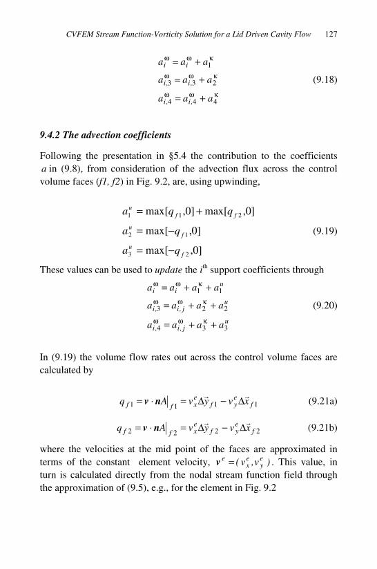
CVFEM Stream Function-Vorticity Solution for a Lid Driven Cavity Flow
127
κωω
κωω
κωω
+=
+=
+=
444
233
1
aaa
aaa
aaa
,i,i
,i,i
ii
(9.18)
9.4.2 The advection coefficients
Following the presentation in §5.4 the contribution to the coefficients
a in (9.8), from consideration of the advection flux across the control
volume faces (f1, f2) in Fig. 9.2, are, using upwinding,
]0,max[
]0,max[
]0,max[]0,max[
23
12
211
f
u
f
u
ff
u
qa
qa
qqa
−=
−=
+=
(9.19)
These values can be used to update the ith support coefficients through
uj,i,i
uj,i,i
uii
aaaa
aaaa
aaaa
334
223
11
++=
++=
++=
κωω
κωω
κωω
(9.20)
In (9.19) the volume flow rates out across the control volume faces are
calculated by
1111 feyf
exff xvyvAq
∆−∆=⋅= nv (9.21a)
2222 feyf
exff xvyvAq
∆−∆=⋅= nv (9.21b)
where the velocities at the mid point of the faces are approximated in
terms of the constant element velocity, )v,v(ey
ex
e =v . This value, in
turn is calculated directly from the nodal stream function field through
the approximation of (9.5), e.g., for the element in Fig. 9.2

Basic Control Volume Finite Element Methods for Fluids and Solids
128
43
43
321
321
,i,i
,i,i
SxSxixey
SySyiyex
NNNv
NNNv
Ψ−Ψ−Ψ−≈
Ψ+Ψ+Ψ≈ (9.22)
This coupling with the nodal stream-function field will require an
iterative solution of (9.16). At each iteration, the advection coefficients
in (9.19) will need to be evaluated to reflect the updating of the iterative
values of the nodal stream-function field.
9.4.3 Boundary conditions
Before (9.16) can be solved boundary conditions need to be prescribed.
Fixed value boundary conditions are used. At each node i on a domain
boundary the discrete form of the stream function equation (9.3) can be
used to prescribe a value for the nodal vorticity. Use of this equation is
allowed since, due to the fact that the stream function takes the known
fixed value 0=Ψ on all boundaries, it is not needed in the stream
function solution. At a node i on the boundary the control volume finite
element discretization of (9.3), informed by (9.8), can be written as
⋅Ψ∇−Ψ−Ψ=ω ∑∑
=
ΨΨ
bounday
n
j
Sj,iiii
i AaaV
i
j,in
1
1 (9.23)
where the coefficients Ψa are given by (9.10) and the definition of the
source term in (9.14) has been used to isolate iω . The last term in (9.23)
represents contributions from control volume faces that coincide with a
boundary segment, see the double line in Fig 9.3. In the sliding lid
problem of Fig. 9.1 the only non-zero contribution from this term will be
for nodes on the sliding lid and will have the form
UA
bounday
∆=
⋅Ψ∇∑ n (9.24)
where ∆ is the length of the control volume surface on the boundary
segment, see Fig. 9.3.

CVFEM Stream Function-Vorticity Solution for a Lid Driven Cavity Flow
129
Fig. 9.3 Node point on sliding lid boundary
Hence, with current iterative values of the stream function known, (9.23)
and (9.24) can be used to estimate fixed nodal values of vorticity for
boundary nodes i
∈∆
−Ψ−Ψ=ω ∑=
ΨΨ
otherwise0
1
1
lidiUaa
V
in
j
Sj,iiii
i
i
j,i (9.25)
These values are forced into the solution of (9.16) by setting
1515 1010 =×ω= ωω
ii CiBB,B
9.5 Solution Steps
9.5.1 Nested iteration
As noted an iterative solution of the coupled equations (9.8) and (9.16) is
required. This is achieved with a nested iteration loop.
iLocal 1
Global Si,1
Local 2
Global Si,2
Local 3
Global Si,3
∆
iLocal 1
Global Si,1
Local 2
Global Si,2
Local 3
Global Si,3
∆
Basic Control Volume Finite Element Methods for Fluids and Solids
130
An outer iteration is made 1- outer (~1000)
With the current best estimates the boundary values of iω are
obtained from (9.25)
The coefficients in (9.16) are calculated.
Equation (9.16) is solved by a simple point iteration scheme; 20
inner iteration steps are used.
The coefficients for (9.8) are calculated; the latest iterative
values of the vorticity are used.
Equation (9.8) is solved by a simple point iteration scheme; 20
inner iteration steps are used.
The default choice of 1000 iterations is usually enough to ensure
convergence. A more sophisticated approach could use a
convergence check to determine the outer iteration closure.
9.5.2 Calculating the nodal velocity field
Following the calculation of the converged Ψ field the nodal velocity
field v can be calculated. Integrating (9.5) over the thi control volume
results in
∫∫∫∫ ∂
Ψ∂−=
∂
Ψ∂=
iiii VV
y
VV
x ,dVx
dVv,dVy
dVv (9.26)
or using the divergence theorem
∫∫∫∫ Ψ−=Ψ=
S
x
V
y
S
y
V
x ndVv,dSndVv
ii
(9.27)
where the surface integral is over the control volume faces, and
)n,n( yx=n is the outward pointing normal on the control volume face.
Using mid point integration approximations

CVFEM Stream Function-Vorticity Solution for a Lid Driven Cavity Flow
131
∑∑ Ψ−=Ψ=faces
xi
y
faces
yi
x AnV
v,AnV
vii
11 (9.28)
where A is the area (length × unit depth) of a given control volume face,
and , since boundary values of 0=Ψ , the summations are restricted to
control faces that do not coincide with the domain boundaries. On
recalling that the outward normal area product on a volume face is
xAn,yAn yx
∆−=∆=
see (9.11) for definitions of xy
∆∆ and , the contributions to control
volume i from the right hand side of (9.28), for the selected element
from the control volume in Fig. 9.2, can be calculated as
2125
122
125
1122
125
125
21
2125
122
125
1122
125
125
21
43
43
43
43
fSSi
fSSi
f,f
x
fSSi
fSSi
f,f
y
y)(
y)(An
x)(
x)(An
,i,i
,i,i
,i,i
,i,i
∆Ψ+Ψ+Ψ
−∆Ψ+Ψ+Ψ−=Ψ
∆Ψ+Ψ+Ψ
−∆Ψ+Ψ+Ψ−=Ψ
∑
∑
(9.29)
With the nodal velocity field calculated from (9.28) the velocity at
given point )yx,(=x can be determine by determining the triangular
element (local nodes 1,2, and 3) which contains the point x and then
using the shape function interpolations
321
321
321
321
yyyy
xxxx
vNvNvN)(v
vNvNvN)(v
++=
++=
x
x (9.30)
Where the shape function iN ( i = 1,2 ,3) are defined in (3.7) and (3.8).

Basic Control Volume Finite Element Methods for Fluids and Solids
132
9.6 Results
For all results, unless otherwise stated, the settings 11 == L,U will be
made; in this way the Reynolds number of the Flow will be ν= /Re 1 .
The calculated flow-field, given by the stream-lines, when 400=Re is
shown in Fig. 9.1. This calculation was carried out on a structured mesh
with 61 rows and 61 columns; a section of this grid is shown in Fig 9.4.
Fig. 9.4 Section of structured 61×61 grid
Ghia, Ghia and Shin (1982) tabulate the benchmark xv velocity
along the line x = 0.5 and the yv velocity along the line y = 0.5 for
Reynolds numbers of 400 and 100=Re . Fig. 9.5 compares the tabulated
100=Re velocities with the calculated velocities based on the CVFEM
stream-function—vorticity solution on the structured grid of Fig. 9.4.
The agreement between the CVFEM and the benchmark is close.
Fig. 9.6 compares the tabulated 400=Re velocities with the calculated
velocities based on the CVFEM stream-function—vorticity solution on
the structured grid of Fig. 9.4. In this case, the agreement between the
CVFEM and the benchmark, although still reasonable, is not as close as
the 100=Re case. This indicates that a finer grid is needed or a more
sophisticated treatment of the vorticity boundary condition.
In contrast to the structured grid results of Figs. 9.1, 9.5 and 9.6, the
CVFEM stream-function—vorticity solution on the unstructured mesh of
Fig. 9.7, for 100=Re , are compared with the tabulated benchmark in
Fig. 9.8. The quality of these predictions is consistent with the structured
grid values of Fig. 9.5.

CVFEM Stream Function-Vorticity Solution for a Lid Driven Cavity Flow
133
Fig. 9.5a u-velocity in sliding lid cavity along x = 0.5. Re =100, structured grid of
Fig. 9.4. Symbols benchmark solution Ghia et al. (1982), lines CVFEM solution
Fig. 9.5b v-velocity in sliding lid cavity along y = 0.5. Re =100, structured grid of
Fig. 9.4. Symbols benchmark solution Ghia et al. (1982), lines CVFEM solution
-0.6
-0.4
-0.2
0
0.2
0.4
0.6
0.8
1
0 0.2 0.4 0.6 0.8 1
-0.6
-0.5
-0.4
-0.3
-0.2
-0.1
0
0.1
0.2
0.3
0.4
0 0.2 0.4 0.6 0.8 1

Basic Control Volume Finite Element Methods for Fluids and Solids
134
Fig. 9.6a u-velocity in sliding lid cavity along x = 0.5. Re =400, structured grid of
Fig. 9.4. Symbols benchmark solution Ghia et al. (1982), lines CVFEM solution.
Fig. 9.6b v-velocity in sliding lid cavity along y = 0.5 (Re = 400, structured grid)
Symbols benchmark solution Ghia et al. (1982), lines CVFEM solution.
-0.6
-0.4
-0.2
0
0.2
0.4
0.6
0.8
1
0 0.2 0.4 0.6 0.8 1
-0.6
-0.4
-0.2
0
0.2
0.4
0 0.2 0.4 0.6 0.8 1

CVFEM Stream Function-Vorticity Solution for a Lid Driven Cavity Flow
135
Fig. 9.7 Unstrctured mesh for stream-function—vorticity CVFEM solution
Fig. 9.8a u-velocity in sliding lid cavity along x = 0.5. Re =100, unstructured grid of
Fig. 9.7 Symbols benchmark solution Ghia et al. (1982), lines CVFEM solution
0 0.2 0.4 0.6 0.8 10
0.1
0.2
0.3
0.4
0.5
0.6
0.7
0.8
0.9
1
-0.6
-0.4
-0.2
0
0.2
0.4
0.6
0.8
1
0 0.2 0.4 0.6 0.8 1

Basic Control Volume Finite Element Methods for Fluids and Solids
136
Fig. 9.8b v-velocity in sliding lid cavity along y = 0.5. Re = 100, unstructured grid of
Fig. 9.7 Symbols benchmark solution Ghia et al. (1982), lines CVFEM solution
Since the CVFEM solution can fit arbitrary geometries it is interesting to
apply it to a modification of the sliding lid problem. One possible
variation is to use a ¼ annulus cavity. An unstructured mesh and
geometry for this problem is shown in Fig. 9.9. Flow in the cavity is
generated by sliding the top lid at a constant x-velocity of 1=xu . Using
the thickness of the annulus ( 1=t ) as the length the viscosity is chosen
to set the Reynolds number at 100=Re . The predictions from the
CVFEM stream-function—vorticity solution are presented as streamlines
in Fig. 9.10; the stream lines in this plot are in the clockwise direction
(negative) and vary from 00001002004006008010 .,.,.,.,.,. −−−−−−=ψ .
This solution is a sound illustration of the power of the CVFEM method
to solve complex problems in arbitrary domains.
-0.6
-0.5
-0.4
-0.3
-0.2
-0.1
0
0.1
0.2
0.3
0.4
0 0.2 0.4 0.6 0.8 1

CVFEM Stream Function-Vorticity Solution for a Lid Driven Cavity Flow
137
Fig. 9.9 Unstructured grid and geometry for annulus sliding lid problem
Fig. 9.10 Negative streamlines (~0 to -0.1) predicted by CVFEM for mesh of Fig. 9.9
0 0.5 1 1.5 2−2
−1.8
−1.6
−1.4
−1.2
−1
−0.8
−0.6
−0.4
−0.2
0
0 0.5 1 1.5 2
−1.8
−1.6
−1.4
−1.2
−1
−0.8
−0.6
−0.4
−0.2
0
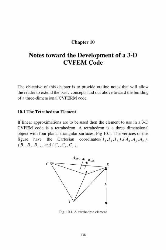
138
Chapter 10
Notes toward the Development of a 3-D
CVFEM Code
The objective of this chapter is to provide outline notes that will allow
the reader to extend the basic concepts laid out above toward the building
of a three-dimensional CVFERM code.
10.1 The Tetrahedron Element
If linear approximations are to be used then the element to use in a 3-D
CVFEM code is a tetrahedron. A tetrahedron is a three dimensional
object with four planar triangular surfaces, Fig 10.1. The vertices of this
figure have the Cartesian coordinates )I,I,I( zyx , )A,A,A( zyx ,
)B,B,B( zyx , and )C,C,C( zyx .
Fig. 10.1 A tetrahedron element
A
B C
I
AABC nABC
h
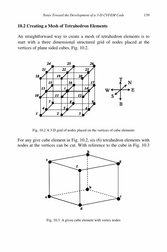
Notes Toward the Development of a 3-D CVFEM Code
139
10.2 Creating a Mesh of Tetrahedron Elements
An straightforward way to create a mesh of tetrahedron elements is to
start with a three dimensional structured grid of nodes placed at the
vertices of plane sided cubes, Fig. 10.2.
Fig. 10.2 A 3-D grid of nodes placed on the vertices of cube elements
For any give cube element in Fig. 10.2, six (6) tetrahedron elements with
nodes at the vertices can be cut. With reference to the cube in Fig. 10.3
Fig. 10.3 A given cube element with vertex nodes
7 8 9
18 19 20
21 22 23
24 25 26
i
1 2 3
4 5 6
10 11 12
13 14
15 16 17T
B
N
S
W E
7 8 9
18 19 20
21 22 23
24 25 26
i
1 2 3
4 5 6
10 11 12
13 14
15 16 17
7 8 9
18 19 20
21 22 23
24 25 26
i
1 2 3
4 5 6
10 11 12
13 14
15 16 17T
B
N
S
W E
T
B
N
S
W E
d
b
a c
e
f
g
h
d
b
a c
e
f
g
h
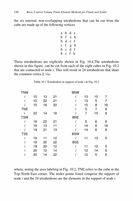
Basic Control Volume Finite Element Methods for Fluids and Solids 140
the six internal, non-overlapping tetrahedrons that can be cut from the
cube are made up of the following vertices
a b d e
b f e h
b d e f
c f g h
b c d f
b c f h
These tetrahedrons are explicitly shown in Fig. 10.4.The tetrahedrons
shown in this figure can be cut from each of the eight cubes in Fig. 10.2
that are connected to node i. This will result in 24 tetrahedrons that share
the common vertex I, viz,
Table 10.1 Tetrahedron in support of node i in Fig. 10.2
TNW BNW
i 15 13 21 i 13 15 7
i 15 22 21 i 13 5 7
i 15 16 22 i 15 8 16
TNE i 5 7 8
i 22 14 16 i 7 15 8
TSW BNE
i 19 22 21 i 5 6 8
i 19 13 11 i 14 8 16
i 19 21 13 i 14 6 8
TSE BSW
i 19 11 12 i 11 13 5
i 19 20 22 BSE
i 19 20 12 i 11 12 5
i 20 12 14 i 12 14 6
i 20 14 22 i 12 5 6
where, noting the axes labeling in Fig. 10.2, TNE refers to the cube in the
Top North East corner. The nodes points listed comprise the support of
node i and the 24 tetrahedrons are the elements in the support of node i.

Notes Toward the Development of a 3-D CVFEM Code
141
Fig. 10.4a Tetrahedrons cut from left hand side
d
b
a c
e
f
g
h
a b d e
d
b
a c
e
f
g
h
b f e h
d
b
a c
e
f
g
h
b d e f
d
b
a c
e
f
g
h
d
b
a c
e
f
g
h
a b d e
d
b
a c
e
f
g
h
b f e h
d
b
a c
e
f
g
h
b f e h
d
b
a c
e
f
g
h
b d e f
d
b
a c
e
f
g
h
d
b
a c
e
f
g
h
b d e f

Basic Control Volume Finite Element Methods for Fluids and Solids 142
Fig. 10.4b Tetrahedrons cut from right hand side
d
b
a c
e
f
g
h
c f g h
a
d
b
c
e
f
g
h
b c d f
d
b
a c
e
f
g
h
b c f h
d
b
a c
e
f
g
h
d
b
a c
e
f
g
h
c f g h
a
d
b
c
e
f
g
h
b c d f
d
b
a c
e
f
g
h
b c f h
c f g h
a
d
b
c
e
f
g
h
b c d f
a
d
b
c
e
f
g
h
b c d f
d
b
c
e
f
g
h
b c d f
d
b
a c
e
f
g
h
b c f h
d
b
a c
e
f
g
h
b c f h

Notes Toward the Development of a 3-D CVFEM Code
143
10.3 Geometric Features of Tetrahedrons
To move forward it is necessary to provide calculations for key
geometric features of a tetrahedron. The volume is given by AhV31=
where A is the area of a given triangular surface and h is the
perpendicular distance from that side to the opposite vertex. In words,
with reference to Fig. 10.1,
Volume = ×31 Area of Surface (ABC) × perpendicular distance from
(ABC) to I
If the vectors from a fixed origin to the vertices of the tetrahedron in Fig
10.1 are
)C,C,C(
)C,B,B(
)A,A,A(
)I,I,I(
zyx
zyx
zyx
zyx
=
=
=
=
C
B
A
I
(i) the vector product )()( ACAB −×−21 gives a vector with
magnitude equal to the area of the surface ABC and direction normal to
the surface ABC , and (ii) the dot product 0>⋅−= ABCnIA )(h , where
ABCn is the unit normal on ABC that points out of tetrahedron IABC ,
gives the height (perpendicular distance) from the surface ABC to vertex
I. In this way, on reference to the word equation given above the volume
of the tetrahedron can be written as
)(
))()(()(T,TV II
CBA
ACABIA
×⋅=
−×−⋅−== where61
(10.1a)
with a clockwise rotation of the vertices I, A , B, and C the volume can
also be calculated with any one of the following
))()(()(T,TV
))()(()(T,TV
))()(()(T,TV
CC
BB
AA
IBΙΑCI
CACIBC
BIBCAB
−×−⋅−==
−×−⋅−==
−×−⋅−==
where
where
where
61
61
61
(10.1b)

Basic Control Volume Finite Element Methods for Fluids and Solids 144
For future use, it is also noted that, the vector
<−×−−
>−×−=
0
0
I
I
T),()(
T),()(
ACAB
ACABAABC (10.2a)
has magnitude equal to the ×2 area of the surface ABC and direction
along the outward pointing normal ABCn . By a clockwise rotation the
vectors
<−×−−
>−×−=
0
0
A
ABCI
T,)()(
T,)()(
BIBC
BIBCA (10.2b)
<−×−−
>−×−=
0
0
B
BCIA
T),()(
T),()(
CACI
CACIA (10.2c)
<−×−−
>−×−=
0
0
C
CIAB
T),()(
T,)()(
IBΙΑ
IBΙΑA (10.2d)
are the counterparts for the surfaces BCI, CIA, and IAB respectively;
each vector pointing out of the tetrahedron IABC in the direction of the
surface unit normals.
Fig. 10.5 Construction for volume shape function at node I
10.4 Volume Shape Functions
The concept of the area shape function can be generalized to three-
dimensions using volume shape functions. For know nodal values of a
quality C,BAI ,, φφφφ the value of φ at any point with position vector X
within the tetrahedron element of Fig. 10.5 can be approximated by
A
B
C
I
X
A
B
C
I
X
Notes Toward the Development of a 3-D CVFEM Code
145
the linear interpolation
BVBB
VBA
VAI
VI NNNN φ+φ+φ+φ=φ (10.3)
where the VN are the volume shape functions defined by
I
VI
T
))()).(((N
ACABXA −×−−==
IABC
XABC
Volume
Volume (10.4a)
C
VC
B
VB
A
VA
T
))()(()(N
T
))()(()(N
T
))()(()(N
IBΙΑXI
CACIXC
BIBCXB
−×−⋅−=
−×−⋅−=
−×−⋅−=
(10.4b)
Note by the construction of the VN ,
∑=
=
C,B,A,IJ
VjN 1
throughout the element, and the shape function associated with the vertex
)CB,A,I(J or vanishes on the opposite element surface. The
derivatives of the shape function associated with vertex I (constant
within the element) are given by
[ ]
[ ]
[ ]
I
zVIz
I
yVIy
I
xVIx
T
))N
T
))N
T
))N
A(CA)((B
A(CA)((B
A(CA)((B
−×−−=
−×−−=
−×−−=
(10.5a)
where [ ]xr indicates the x-component of the vector r. Similar
expressions for the derivatives of the three remaining shape functions can
be readily obtained from (10.4b).
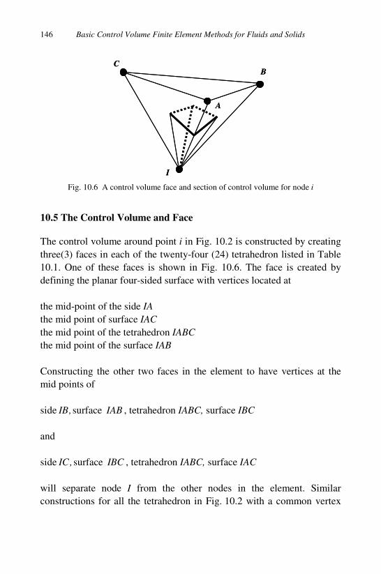
Basic Control Volume Finite Element Methods for Fluids and Solids 146
Fig. 10.6 A control volume face and section of control volume for node i
10.5 The Control Volume and Face
The control volume around point i in Fig. 10.2 is constructed by creating
three(3) faces in each of the twenty-four (24) tetrahedron listed in Table
10.1. One of these faces is shown in Fig. 10.6. The face is created by
defining the planar four-sided surface with vertices located at
the mid-point of the side IA
the mid point of surface IAC
the mid point of the tetrahedron IABC
the mid point of the surface IAB
Constructing the other two faces in the element to have vertices at the
mid points of
side ,IB surface IAB , tetrahedron IABC, surface IBC
and
side ,IC surface IBC , tetrahedron IABC, surface IAC
will separate node I from the other nodes in the element. Similar
constructions for all the tetrahedron in Fig. 10.2 with a common vertex
A
BC
I
A
BC
I
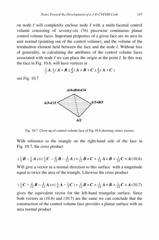
Notes Toward the Development of a 3-D CVFEM Code
147
on node I will completely enclose node I with a multi-faceted control
volume consisting of seventy-six (76) piecewise continuous planar
control volume faces. Important properties of a given face are its area its
unit normal (pointing out of the control volume), and the volume of the
tetrahedron element held between the face and the node I. Without loss
of generality, in calculating the attributes of the control volume faces
associated with node I we can place the origin at the point I. In this way
the face in Fig. 10.6, will have vertices at
)(),(),(, CACBABAA31
41 ++++
31
21
see Fig. 10.7
Fig. 10.7 Close up of control volume face of Fig 10.6 showing vertex vectors
With reference to the triangle on the right-hand side of the face in
Fig. 10.7, the cross product
ACBACBABCAB 11 ×+×+×=−−×−241
241
121
121241
61
31 )()( (10.6)
Will give a vector in a normal direction to this surface with a magnitude
equal to twice the area of the triangle. Likewise the cross product
ACBACBCAABC 11 ×+×+×=−×−−241
241
121
31
61
121241 )()( (10.7)
gives the equivalent vector for the left-hand triangular surface. Since
both vectors in (10.6) and (10.7) are the same we can conclude that the
construction of the control volume face provides a planar surface with an
area normal product
A/2
A/3+B/3
A/4+B/4+C/4
A/3+C/3
A/2
A/3+B/3
A/4+B/4+C/4
A/3+C/3
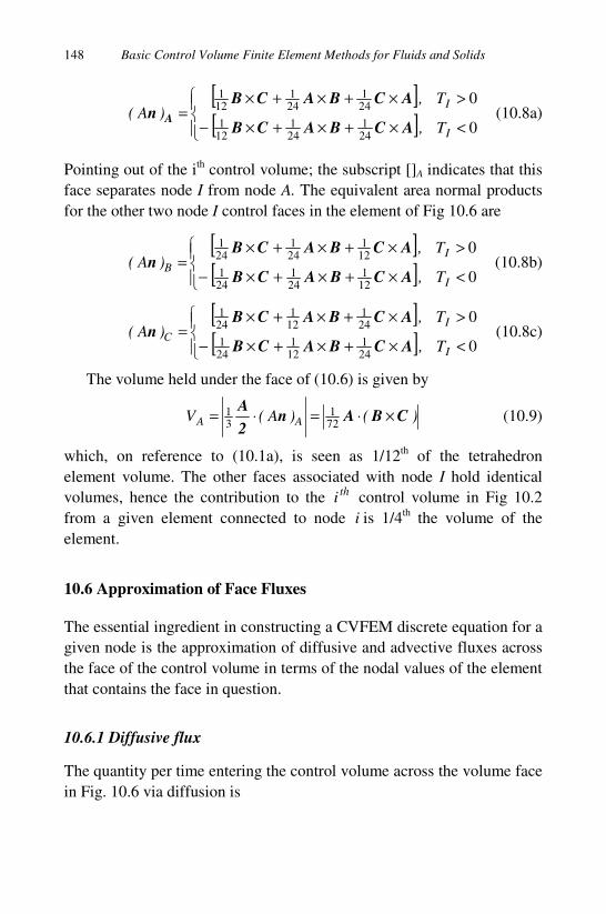
Basic Control Volume Finite Element Methods for Fluids and Solids 148
[ ][ ]
<×+×+×−
>×+×+×=
0
0
241
241
121
241
241
121
I
I
T,
T,)A(
ACBACB
ACBACBn A (10.8a)
Pointing out of the ith control volume; the subscript []A indicates that this
face separates node I from node A. The equivalent area normal products
for the other two node I control faces in the element of Fig 10.6 are
[ ][ ]
<×+×+×−
>×+×+×=
0
0
121
241
241
121
241
241
I
I
BT,
T,)A(
ACBACB
ACBACBn (10.8b)
[ ][ ]
<×+×+×−
>×+×+×=
0
0
241
121
241
241
121
241
I
I
CT,
T,)A(
ACBACB
ACBACBn (10.8c)
The volume held under the face of (10.6) is given by
)()A(V AA CBAn2
A×⋅=⋅=
721
31 (10.9)
which, on reference to (10.1a), is seen as 1/12th of the tetrahedron
element volume. The other faces associated with node I hold identical
volumes, hence the contribution to the thi control volume in Fig 10.2
from a given element connected to node i is 1/4th the volume of the
element.
10.6 Approximation of Face Fluxes
The essential ingredient in constructing a CVFEM discrete equation for a
given node is the approximation of diffusive and advective fluxes across
the face of the control volume in terms of the nodal values of the element
that contains the face in question.
10.6.1 Diffusive flux
The quantity per time entering the control volume across the volume face
in Fig. 10.6 via diffusion is
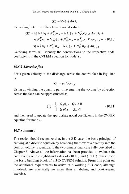
Notes Toward the Development of a 3-D CVFEM Code
149
ADA )A(Q n⋅φ∇κ=
Expanding in terms of the element nodal values
AzCVCzB
VBzA
VAzI
VIz
AyCVCyB
VByA
VAyI
VIy
AxCVCxB
VBxA
VAxI
VIx
DA
)An)(NNNN(
)An)(NNNN(
)An)(NNNN(Q
φ+φ+φ+φκ
+φ+φ+φ+φκ
+φ+φ+φ+φκ=
(10.10)
Gathering terms will identify the contributions to the respective nodal
coefficients in the CVFEM equation for node I .
10.6.2 Advective flux
For a given velocity v the discharge across the control face in Fig. 10.6
is
AA )A(Q nv ⋅=
Using upwinding the quantity per time entering the volume by advection
across the face can be approximated as
<φ−
>φ−=
0
0
AAA
AIAUA
Q,Q
Q,QQ (10.11)
and then used to update the appropriate nodal coefficients in the CVFEM
equation for node i .
10.7 Summary
The reader should recognize that, in the 3-D case, the basic principal of
arriving at a discrete equation by balancing the flow of a quantity into the
control volume is identical to the two-dimensional case fully described in
Chapter 5. Above all the information has been provided to evaluate the
coefficients on the right-hand sides of (10.10) and (10.11). These form
the basic building block of a 3-D CVFEM solution. From this point on,
the additional requirements to arrive at a working 3-D code, although
involved, are essentially no more than a labeling and bookkeeping
exercise.
150
Appendix A
A Meshing Code
This appendix provides a MATLAB code (MESH.m) for creating a mesh
of linear triangular elements. The data structure generated matches the
unstructured data structure presented in Chapter 3 and used in the
CVFEM developments in Chapter 5. Note, however, that this mesh is
generated by initially assuming that the nodes points are laid out on a
structured grid of rows and columns. On the grid the morphology of the
region of support i always have the morphology shown in Fig. A1.
Further, the application of this code is limited to domains with 4 distinct
sides that can be covered by a grid of rows and columns. The obvious
domains are rectangles and squares, but with some imagination it is
possible to find and mesh other domains that have a similar morphology;
two important examples, illustrated in Fig. A.2, are an annulus (a ¼
section is shown) and a plate with a hole (an 1/8 section is shown).
Please note:
(1) The code MESH is not an attempt to win the MATLAB program of
the year. Indeed, the author has purposely attempted to write the
most basic code, avoiding, where possible, any build in MATLAB
functions and efficiencies. Hence the resulting code may not be
efficient but it is understandable and will allow for the translation to
other coding languages.
(2) The code MESH is provided so that readers can get a rapid start on
programming and using the CVFEM. In more general application the
experienced reader is encouraged to use an alternative un-structured
mesh generator followed by an appropriate “translation” to generate
the data structure outlined in Chapter 3.
(3) The mesh generated is given in Fig. B1. (appendix B).

A Meshing Code 151
Fig. A1 The assumed morphology of the region of support in the program MESH
%MESH
%V.R. Voller
%This program creates a triangular mesh and its data structure
%From a row-col(umn) structure laid out on a 4-sided domain
%The 1/4 annulus domain( see Fig A2) is programmed here
clear all
rows=21;
cols=21;
n=rows*cols; %Total domain nodes
% Global nodes points stored in vectors x and y
% Current settings for 1/4 annulus
rin=1; %inner radius
i i+1
i+1+cols i+cols
i-1
i-1-cols i-cols
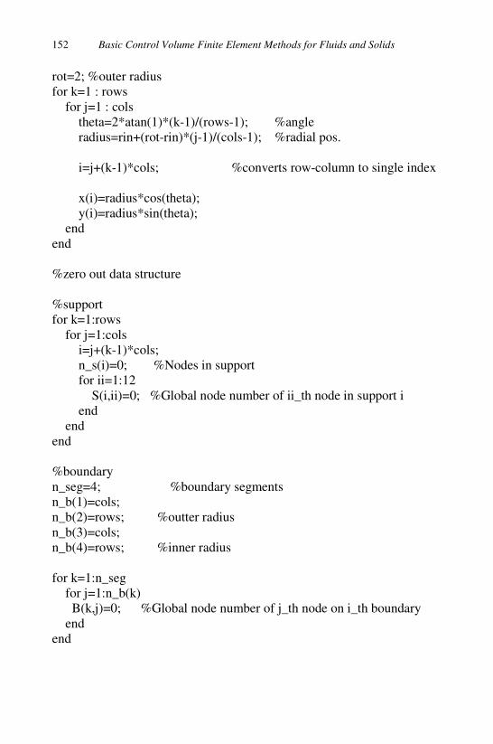
Basic Control Volume Finite Element Methods for Fluids and Solids 152
rot=2; %outer radius
for k=1 : rows
for j=1 : cols
theta=2*atan(1)*(k-1)/(rows-1); %angle
radius=rin+(rot-rin)*(j-1)/(cols-1); %radial pos.
i=j+(k-1)*cols; %converts row-column to single index
x(i)=radius*cos(theta);
y(i)=radius*sin(theta);
end
end
%zero out data structure
%support
for k=1:rows
for j=1:cols
i=j+(k-1)*cols;
n_s(i)=0; %Nodes in support
for ii=1:12
S(i,ii)=0; %Global node number of ii_th node in support i
end
end
end
%boundary
n_seg=4; %boundary segments
n_b(1)=cols;
n_b(2)=rows; %outter radius
n_b(3)=cols;
n_b(4)=rows; %inner radius
for k=1:n_seg
for j=1:n_b(k)
B(k,j)=0; %Global node number of j_th node on i_th boundary
end
end

A Meshing Code 153
%SUPPORT DATA ------------
%Assumed Morphology in Fig. A1
% Support for internal points
for k=2:rows-1
for j=2:cols-1
i=j+(k-1)*cols;
n_s(i)=6;
S(i,1)=i+1; %assumed morphology for support see Fig. A1
S(i,2)=i+1+cols;
S(i,3)=i+cols;
S(i,4)=i-1;
S(i,5)=i-1-cols;
S(i,6)=i-cols;
S(i,7)=i+1; %last node is same as first node at internal nodes
end
end
%horizonal boundary (y=0) Non-corner points
for j=2:cols-1
i=j;
n_s(i)=4;
S(i,1)=i+1; % arranged so that points are--
S(i,2)=i+1+cols; % --contiguous in counter clockwise count
S(i,3)=i+cols;
S(i,4)=i-1;
S(i,5)=0; % last point zero: a boundary node flag
end
%outter (rot) curve boundary Non-corner points
for k=2:rows-1
i=cols+(k-1)*cols;
n_s(i)=4;
S(i,1)=i+cols;
S(i,2)=i-1;

Basic Control Volume Finite Element Methods for Fluids and Solids 154
S(i,3)=i-1-cols;
S(i,4)=i-cols;
S(i,5)=0;
end
% vertical boundary (x=0) Non-corner points
for j=2:cols-1
i=j+(rows-1)*cols;
n_s(i)=4;
S(i,1)=i-1;
S(i,2)=i-1-cols;
S(i,3)=i-cols;
S(i,4)=i+1;
S(i,5)=0;
end
%inner (rin) curve boundary Non-corner points
for k=2:rows-1
i=1+(k-1)*cols;
n_s(i)=4;
S(i,1)=i-cols;
S(i,2)=i+1;
S(i,3)=i+1+cols;
S(i,4)=i+cols;
S(i,5)=0;
end
%Corners
% x=0, y = rin
i=1;
n_s(i)=3;
S(i,1)=i+1;
S(i,2)=i+1+cols;
S(i,3)=i+cols;
S(i,4)=0;
% y = 0 x = rot
i=cols;
n_s(i)=2;

A Meshing Code 155
S(i,1)=i+cols;
S(i,2)=i-1;
S(i,3)=0;
% x =0 y = rot
i=rows*cols;
n_s(i)=3;
S(i,1)=i-1;
S(i,2)=i-1-cols;
S(i,3)=i-cols;
S(i,4)=0;
% x=0 y = rin
i=1+(rows-1)*cols;
n_s(i)=2;
S(i,1)=i-cols;
S(i,2)=i+1;
S(i,3)=0;
%END SUPPORT DATA-----------
% BOUNDARY DATA------------
%NOTE counter-clockwise numbering and boundary segment index
% y=0 boundary (segment 1)
for i=1:n_b(1)
B(1,i)=i;
end
% r=rout boundary (segment 2)
for i=1:n_b(2)
B(2,i)=i*cols;
end
% x =0 boundary (segment 3)
for i=1:n_b(3)
B(3,i)=rows*cols+1-i;
end
Basic Control Volume Finite Element Methods for Fluids and Solids 156
% r=rin boundary (segment 4)
for i=1:n_b(4)
B(4,i)=1+rows*cols-i*cols;
end
%END BOUNDARY DATA------------------
%Print Out mesh from supports (MATLAB functions used)
hold on
axis equal
for i=1:n
clear xtemp;
clear ytemp;
ytemp(1)=y(i);
xtemp(1)=x(i);
for j=1:n_s(i)
xtemp(2)=x(S(i,j));
ytemp(2)=y(S(i,j));
plot(xtemp,ytemp,'k');
end
end
%hold off
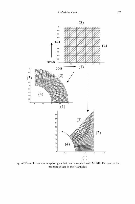
A Meshing Code 157
Fig. A2 Possible domain morphologies that can be meshed with MESH. The case in the
program given is the ¼ annulus
0 0.5 1 1.5 20
0.2
0.4
0.6
0.8
1
1.2
1.4
1.6
1.8
2
0.5 1 1.5 2 2.50
0.2
0.4
0.6
0.8
1
1.2
1.4
1.6
1.8
1 1.2 1.4 1.6 1.8 20
0.1
0.2
0.3
0.4
0.5
0.6
0.7
0.8
0.9
1
(1)
(2)
(3)
(4)
(1)
(2)
(3)
(4)
(2)
(3)
(4)
(1)
rows
cols

158
Appendix B
A CVFEM Code
This appendix provides a MATLAB code (CVFEM.m) that implements a
CVFEM solution for the steady state advection diffusion in an annulus.
The full problem definition is given in §7.7.2. Here the governing
equation is written in two-dimensional Cartesian form
,yyxxy
v
x
v yx 0=
∂
φ∂κ
∂
∂−
∂
φ∂κ
∂
∂−
∂
φ∂+
∂
φ∂
in
2100 22 ≤+≤≥≥ yx,y,x
With boundary conditions
11 22 =+=φ yxon, , 20 22 =+=φ yxon,
00 ==∂
φ∂yon,
y, 00 ==
∂
φ∂xon,
x
and parameter definitions
)x/y(tan,
yx
)sin(v,
yx
)cos(v,
yxyx
1
222222
1 −=θ+
θ=
+
θ=
+=κ
This equation is solved in the code CVFEM using the mesh and data
structure generated by the program MESH in Appendix A. The domain
and the mesh used is shown in Fig. B1.
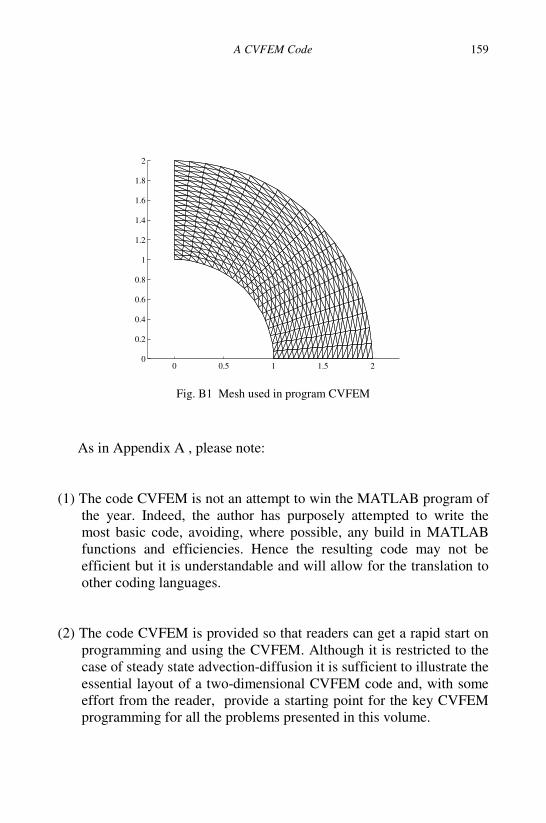
A CVFEM Code 159
Fig. B1 Mesh used in program CVFEM
As in Appendix A , please note:
(1) The code CVFEM is not an attempt to win the MATLAB program of
the year. Indeed, the author has purposely attempted to write the
most basic code, avoiding, where possible, any build in MATLAB
functions and efficiencies. Hence the resulting code may not be
efficient but it is understandable and will allow for the translation to
other coding languages.
(2) The code CVFEM is provided so that readers can get a rapid start on
programming and using the CVFEM. Although it is restricted to the
case of steady state advection-diffusion it is sufficient to illustrate the
essential layout of a two-dimensional CVFEM code and, with some
effort from the reader, provide a starting point for the key CVFEM
programming for all the problems presented in this volume.
0 0.5 1 1.5 20
0.2
0.4
0.6
0.8
1
1.2
1.4
1.6
1.8
2
Basic Control Volume Finite Element Methods for Fluids and Solids
160
%CVFEM
%V.R. Voller
%current set up steady-state advection-diffusion in a 1/4 annulus.
%Mesh and data structure obtained from program MESH.m
%The inner (r = 1) radius is fixed at the value 1
%The outer radius (r = 2) is fixed at the value 0
%The radial velocity is v_r = 1/r
%The diffusivity is kappa=1/r
%radial value and angle
for i=1:n
radius(i)=sqrt(x(i)^2+y(i)^2); % radial position
theta(i)=atan2(y(i),x(i)); % angle
end
% x-y Velocity field
for i=1:n
vx(i)=cos(theta(i))/radius(i);
vy(i)=sin(theta(i))/radius(i);
end
% SET CVFEM COEFICIENTS-----------------
%zero out coefficient
for i=1:n %loop on nodes
%zero out coefficient
ap(i)=0.0; %node point coefficient
V(i)=0.0; %volume of CV
for j=1:n_s(i)+1
a(i,j)=0.0; %neighbor coefficient
end

A CVFEM Code 161
% Set loopcount
% At internal nodes--recognized by S(i,n_s(i)+1)<>0
% the nodes in the support match the elements in the support
% Hence loop over every node in the node i support: loopcount=n_s(i)
% At boundary nodes--recognized by S(i,n_s(i)+1)=0
% the nodes in the support are one larger than the elements in the support
% Hence only loop over the first n_s-1 nodes: loopcount=n_s(i)
loopcount=n_s(i);
if S(i,n_s(i)+1)==0
loopcount=n_s(i)-1;
end
% Pick out each element in turn from i_th support
for j=1:loopcount
k1=S(i,j); %The numbers of the nodes in the j_th elemnt are
k2=S(i,j+1); % i, k1=S(i,J), and k2=S(i,j+1)
xL(1) = x(i); %xL=local x-coordinate of a node within a element
xL(2) = x(k1);
xL(3) = x(k2);
yL(1) = y(i); %yL=local y-coordinate of a node within a element
yL(2) = y(k1);
yL(3) = y(k2);
% nodal diffusivity (kappa)
diff(1)=1/sqrt(xL(1)^2+yL(1)^2);
diff(2)=1/sqrt(xL(2)^2+yL(2)^2);
diff(3)=1/sqrt(xL(3)^2+yL(3)^2);

Basic Control Volume Finite Element Methods for Fluids and Solids
162
% nodal velocities
vxL(1)=vx(i);
vxL(2)=vx(k1);
vxL(3)=vx(k2);
vyL(1)=vy(i);
vyL(2)=vy(k1);
vyL(3)=vy(k2);
% Vele= element-volume
Vele=(xL(2)*yL(3)-xL(3)*yL(2)-xL(1)*yL(3)+xL(1)*yL(2)...
+yL(1)*xL(3)-yL(1)*xL(2))/2;
V(i)=V(i)+Vele/3; %Contribution to control volume
Nx(1)= (yL(2)-yL(3))/(2*Vele); %derivative of shape function wrt x
Nx(2)= (yL(3)-yL(1))/(2*Vele);
Nx(3)= (yL(1)-yL(2))/(2*Vele);
Ny(1)=-(xL(2)-xL(3))/(2*Vele); %derivative of shape function wrt y
Ny(2)=-(xL(3)-xL(1))/(2*Vele);
Ny(3)=-(xL(1)-xL(2))/(2*Vele);
% Face 1--values of diffusivity and velocity
diff_f=(5*diff(1)+5*diff(2)+2*diff(3))/12;
vxf= (5*vxL(1)+5*vxL(2)+2*vxL(3))/12;
vyf= (5*vyL(1)+5*vyL(2)+2*vyL(3))/12;
% Face 1--face area normal components
delx= [(xL(1)+xL(2)+xL(3))/3]-[(xL(1)+xL(2))/2];
dely= [(yL(1)+yL(2)+yL(3))/3]-[(yL(1)+yL(2))/2];
qf=vxf*dely-vyf*delx; %Face 1 volume flux
% Face 1--Diffusion Coefficients
ap(i) = ap(i) + diff_f*(- Nx(1) * dely + Ny(1) * delx);
a(i,j) = a(i,j) + diff_f*( Nx(2) * dely - Ny(2) * delx);
a(i,j+1) = a(i,j+1) + diff_f*( Nx(3) * dely - Ny(3) * delx);

A CVFEM Code 163
% Face 1--Advection Coefficients
ap(i)= ap(i) +max(qf,0);
a(i,j)=a(i,j) +max(-qf,0);
% Face 2--values of diffusivity and velocity
diff_f=(5*diff(1)+2*diff(2)+5*diff(3))/12;
vxf=( 5*vxL(1)+2*vxL(2)+5*vxL(3))/12;
vyf=( 5*vyL(1)+2*vyL(2)+5*vyL(3))/12;
% Face 2--face area normal components
delx= [(xL(1)+xL(3))/2]-[(xL(1)+xL(2)+xL(3))/3];
dely= [(yL(1)+yL(3))/2]-[(yL(1)+yL(2)+yL(3))/3];
qf=vxf*dely-vyf*delx;% Face 1 volume flux
% Face 2--Diffusion Coefficients
ap(i) = ap(i) + diff_f*(- Nx(1) * dely + Ny(1) * delx);
a(i,j) = a(i,j) + diff_f*( Nx(2) * dely - Ny(2) * delx);
a(i,j+1) = a(i,j+1) + diff_f*( Nx(3) * dely - Ny(3) * delx);
% Face 2--Advection Coefficients
ap(i)= ap(i) + max(qf,0);
a(i,j+1) = a(i,j+1) + max(-qf,0);
end %end loop on nodes/elements in support
% For internal nodes LAST node in region of support is also the FIRST
% Hence coefficient for last node needs to be added to first node
% and then removed
a(i,1)=a(i,1)+a(i,n_s(i)+1);
a(i,n_s(i)+1)=0;
end %end loop on nodes in domain
% END CVFEM COEFFICIENTS-----------

Basic Control Volume Finite Element Methods for Fluids and Solids
164
%SET BOUNDARY
for i=1:n %Default values
BC(i)=0; %coefficient part
BB(i)=0; %constant part
end
% Set value = 0 on r = r_outer boundary segment 2
for k=1:n_b(2)
BC(B(2,k))=1e18;
end
%set value =1 on r = r_inner boundary segment 4
for k=1:n_b(4)
BC(B(4,k))=1e18;
BB(B(4,k))=1e18;
end
%------------------------------
%SET SOURCE (No source in current problem)
for i=1:n
QC(i)=0;
QB(i)=0;
end
%-------------------------

A CVFEM Code 165
%SOLVER
%Very Crude point iteration Solver
%Caution There is no formal convergence check
%Increase the size of the iteration loop to ensure convergence
%Defualt initial guess
for i=1:n
phi(i)=0; %Dependent variable
end
for iter=1:1500 %Choose sufficient iteration for convergence
for i= 1:n
RHS=BB(i)+QB(i);
for j=1:n_s(i)
RHS=RHS+a(i,j)*phi(S(i,j));
end
phi(i)=RHS/(ap(i)+BC(i)+QC(i));
end
end
%END SOLVRT
%store phi values on x-axis
pout=0;
for i=1:n
if y(i)<1e-5
pout=pout+1;
xout(pout)=x(i);
phiout(pout)=phi(i);
end
end
____________________________________

Basic Control Volume Finite Element Methods for Fluids and Solids
166
Fig. B2 Results from CVFEM (open symbols) compared with analytical solution (line)
The solution from this code, the profile of φ along the x-axis is
compared with the analytical solution
22
2
2
yxr,ee
eer
+=−
−=φ
In Fig. B2. In addition to provide a detailed comparison some point
values are given in Table B1.
Table B1 Comparison of CVFEM and analytical predictions
x CVFEM Analytical
1 1 1
1.2 0.8667 0.871149
1.4 0.706 0.713769
1.6 0.5119 0.521546
1.8 0.2783 0.286764
2 0 0
0
0.2
0.4
0.6
0.8
1
1 1.5 2
Radial Position
Val
ue

167
Bibliography
Abramowitz, M. and Stegun I. A. (1970). Handbook of mathematical functions, Dover,
New York.
Baliga, B.R., and Atabaki, N. (2006). Control-volume-based finite-difference and finite-
element methods, Handbook of Numerical Heat Transfer (eds Minkowycz,W .J.,
Sparrow, E. M, and Murthu, J. Y), Wiley, Hoboken.
Baliga, B.R., and Patankar, S.V. (1980). A new finite element formulation for
convection-diffusion problems, Numer, Heat Transfer, 3, pp. 393-409.
Batchelor, G.K. (1970). An introduction to fluid dynamics, Cambridge University Press.
Barber, J.R. (2003). Elasticity 2nd ed., Kluwer Academic Publishers Dordrecht / Boston.
Crank, J. and Nicolson, P. (1947). A practical method for numerical evaluation of
solutions of partial differential equations of the heat conduction type, Proc.
Cambridge Phil. Soc. 43, pp. 50–64.
Ghia U, Ghia KN, Shin CT. (1982). High-Re solutions for incompressible flow using the
Navier-Stokes equations and a multigrid method, Journal of Computational
Physics, 48, pp.387-411.
Hsieh, P.A. (1986). A new formula for the analytical solution of the radial dispersion
problem, Water Resources Rresearch, 22, pp. 1597-1605.
Kikuchi, N. (1986). Finite element methods in mechanics, Cambridge University Press,
Cambridge.
Fryer, Y.D., Bailey, C. Cross, M. and Lai, C.-H. (1991). A control-volume procedure fro
solving the elastic stress-strain equations on an unstructured mesh, Applied Math.
Model., 15, pp.639-645.
Patankar, S. V. (1980). Numerical heat transfer and fluid flow, Hemisphere, Washington.
Pepper, D. W. (2006). Meshless methods, Handbook of Numerical Heat Transfer (eds
Minkowycz,W .J., Sparrow, E. M, and Murthu, J. Y), Wiley, Hoboken.
Smith G.D. (1985). Numerical solution of partial differential equations: Finite difference
methods (3rd edn.), Oxford University Press.
Winslow, A.M. (1966). Numerical solution of the quasilinear Poisson equation in a
nonuniform triangular mesh, J. Comp. Phys., 1, pp. 149-172.
Basic Control Volume Finite Element Methods for Fluids and Solids 168
Woodfield, P. L., Suzuki, K., and Nakabe, K. (2004). A simple strategy for constructing
bounded convection schemes for unstructured grids, International Journal for
Numerical Methods in Fluids, 46, pp. 1007-1024.
Zienkiewicz, O. C. and Taylor, R. L. (1989). The finite element method (4th edn.),
McGraw-Hill, London.

169
Index
advection, 2
advection coefficients, 48
advection-diffusion, 2, 10-11
advective flux
analytical solutions, 76
area shape function, 27
artificial diffusion, 48
cloud, 25
coefficients, 30
conjugate diffusivity, 62
conservation of a scalar, 9
control volume, 28, 37
control volume finite element method,
2
convection boundary, 57
Crank-Nicolson, 66
data structure, 33
Delaunay triangularization, 25
derivatives of shape functions, 27
domain boundary, 35
diffusion coefficients, 46
diffusive flux, 10
diffusivity, 11
discrete equations, 30, 35
displacement, 12
equations of motion, 7-9
equilibrium, 12
elements, 23
error function, 84
Eulerian frame, 7
explicit time integration, 66
exponential integral, 96
face area, 42
face normal, 43
Fician diffusion, 4
finite difference methods, 1, 69
finite element methods, 1
fixed flux boundary, 59
fixed value boundary,58
flux, 9
Gauss-Seidel iteration, 59
grid, 23
Hooke’s law, 12
implict time integration, 66
incompressible flow, 10
initial strain, 13
insulated boundary, 58
iterative solution, 60
Largrangian, 7
lid driven cavity, 121
line source, 51
linear element, 25
mass conservation, 7
material velocity, 8
mesh, 23
mesh generation, 25, 32
meshless solutions, 25
method of weighted residuals, 22
momentum, 8
Navier-Stokes equations, 18
Newtonian flow, 18

Basic Control Volume Finite Element Methods for Fluids and Solids 170
nodal derivative, 115
nodal lumping, 50
nodal stress field, 119
node points, 22
numerical dispersion, 84
Peclet number, 85
plane strain, 16
plane stress, 14
Possion’s ratio, 13
pressure, 18
recharge well, 100
region of support, 28, 34
relaxation, 60
Reynolds number, 122
shape function,25
small deformation, 12
source linearization, 50
strain rate tensor, 18
stream function, 21
stress tensor, 8
stress concentration, 106
stress in an element, 115
structured grid, 23
thermal expansion, 13
tetrahedron element, 138
tetrahedron normal, 143
tetrahedron mesh, 139
tetrahedron volume, 143
traction, 8
transients, 65
triangular element, 25
under relaxation, 60
unstructured mesh, 23
upwinding, 48
variable diffusivity, 61
velocity, 18, 21
velocity field, 130
viscosity, 18
volume shape function, 144
volume source term, 49
vorticity, 21
Young’s modulus, 13