basic cellular radio engineering document

8/6/2019 Basic Cellular Radio Engineering Document

http://slidepdf.com/reader/full/basic-cellular-radio-engineering-document 1/41

BASIC CELLULAR

RADIO

ENGINEERING

Abstract

This paper is intended to provide a better understanding in basicpropagation theory, cell planning, basic teletraffic theory, basicantenna theory and common RF ancilliaries.



Basic Cel lular Engineer ing CPO2 For Internal Use Only 2

REVISION LIST

Date Revision Description Responsibility Approvals Comments

13rd April 2001 1.0 Initial draft Edwin Yapp




TABLE OF CONTENTS

REVISION LIST.................................................................................................................................................................................................2

1. BASIC PROPAGATION THEORY................................................................................................................................................5

1.1 PROPAGATION BASICS.......................................................................................................................................................................5

1.2 RULE OF THUMB.................................................................................................................................................................................6

1.3 ATTENUATION SLOPE.......................................................................................................................................................................6

1.4 PROPAGATION PROBLEMS................................................................................................................................................................7

1.4.1 Rayleigh Fading......................................................................................................................................................................7

1.4.2 Time Dispersion.......................................................................................................................................................................8

1.4.3 Sh adowing................................................................................................................................................................................9

1.4.4 Diffraction.................................................................................................................................................................................9

1.4.5 Reflection............................................................................................................................................................................... 10

1.4.6 Natural Path Loss ................................................................................................................................................................ 10

1.4.7 Interference ............................................................................................................................................................................10

1.5 PROPAGATION PROBLEMS – SOLUTIONS...................................................................................................................................11

1.5.1 Equalization.......................................................................................................................................................................... 111.5.2 Diversity ................................................................................................................................................................................. 12

1.5.3 Frequency Hopping.............................................................................................................................................................13

1.5.4 Interleaving ...........................................................................................................................................................................13

1.5.5 Channel Coding ................................................................................................................................................................... 14

1.5.6 Discontinuous Transmission/Reception .......................................................................................................................... 15

1.5.7 Dynamic Power Control ..................................................................................................................................................... 15

2. CELL PLANNING...........................................................................................................................................................................17

2.1 NOMINAL CELL PLANNING ............................................................................................................................................................17

2.2 CELL PLANNING TOOL .................................................................................................................................................................... 17

2.3 PROPOGATION MODELS..................................................................................................................................................................18

2.4 THE GRID............................................................................................................................................................................................18

2.5 CELL PLANNING PROCESS............................................................................................................................................................... 19

2.6 CELL PLANNING CONSIDERATIO NS............................................................................................................................................... 20

3. BASIC TELETRAFFIC THEORY................................................................................................................................................ 22

3.1 INTRODUCTION ................................................................................................................................................................................22

3.2 ERLANG TABLES............................................................................................................................................................................... 23

3.3 TRAFFIC CONCEPTS.........................................................................................................................................................................24

3.4 DIMENSIONING A CELL...................................................................................................................................................................24

3.5 SECTORED VS OMNI SITES.......................................................................................................................................................... 25

4. BASIC ANTENNA THEORY........................................................................................................................................................ 28

4.1 INTRODUCTION ................................................................................................................................................................................28

4.2 ISOTROPIC RADIATION.................................................................................................................................................................... 28

4.3 COMMON ANTENNA.........................................................................................................................................................................29

4.4 ANTENNA SPECIFICATIONS ......................................................................................................................................................29

5. COMMON RF ANCILLIARIES ...................................................................................................................................................36

5.1 EQUIPMENT .......................................................................................................................................................................................37

5.1.1 Couplers ................................................................................................................................................................................. 38

5.1.2 Split ters/Combine ................................................................................................................................................................ 39

5.1.3 Fil ters .....................................................................................................................................................................................40

5.1.4 Duplexers............................................................................................................................................................................... 40

5.1.5 Isolators ................................................................................................................................................................................. 41

5.1.6 Cables/Connectors .............................................................................................................................................................. 41

5.1.7 Attenuators ............................................................................................................................................................................41




CHAPTER 1

BASIC PROPAGATION THEORY

Objectives: This chapter will describe the basic studies ofwave propagation, some of the problems

encountered in propagation as well as thesolutions to overcome these problems.

Upon completion of this chapter, the student will be able to:

• Understand the basics of wave propagation• Explain the problems encountered in propagation• Describe the solutions for the propagation problems




1.2 RULE OF THUMB

Furthering the equation above and knowing that

32.4 + 20log2D + 20logF dB = 32.4 + 6 + 20logD + 20logF dB

32.4 + 20log4D + 20logF dB = 32.4 + 6 + 6 +20logD +20logF dB

Hence, at every doubling (octave) of the distance, D, add 6dB/octave.

32.4 + 20log10D + 20logF dB = 32.4 + 20 + 20logD + 20logF dB

32.4 + 20log100D + 20logF dB = 32.4 + 20 + 20 + 20logD +20logF dB

Hence, at every ten-fold (decade) of the distance, D, add 20dB/decade.

1.3 ATTENUATION SLOPE

The FSPL can be re-written as,

FSPL = Lo + 10γ γ log D

Where γ γ is the slope of the attenuation with respect to distance, D.

λ f c =




1.4 PROPAGATION PROBLEMS

1.4.1 Rayleigh Fading

This occurs when a signal takes more than one path between the MS and BTSantennas. In this case, the signal is not received on a line of sight path directly fromthe Tx antenna. Rather, it is reflected off buildings, for example, and is receivedfrom several different indirect paths. Rayleigh fading occurs when the obstaclesare close to the receiving antenna.

The received signal is the sum of many identical signals, which differ only in phase(and to some extent amplitude). A fading dip and the time that elapses betweentwo fading dips depend on both the speed of the MS and the transmittingfrequency. As an approximation, the distance between two dips caused byRayleigh fading is about half a wavelength. Thus, for GSM 900 the distancebetween dips is about 17 cm. Figure 1-2 below shows an example of Rayleigh

fading.

Figure 1-2




1.4.2 Time Dispersion

Time dispersion is another problem relating to multiple paths to the Rx antenna ofeither an MS or BTS. However, in contrast to Rayleigh fading, the reflected signalcomes from an object far away from the Rx antenna.

Time dispersion causes Inter-Symbol Interference (ISI) where consecutivesymbols (bits) interfere with each other making it difficult for the receiver todetermine which symbol is the correct one. An example of this is shown in thefigure below where the sequence 1, 0 is sent from the BTS.

If the reflected signal arrives one bit time after the direct signal, then the receiverdetects a 1 from the reflected wave at the same time it detects a 0 from the directwave. The symbol 1 interferes with the symbol 0 and the MS does not know whichone is correct. This can be shown in Figure 1-3.

Figure 1-3




1.4.3 Shadowing

Shadowing occurs when there are physical obstacles including hills and buildingsbetween the BTS and the MS. The obstacles create a shadowing effect that candecrease the received signal strength. When the MS moves, the signal strengthfluctuates depending on the obstacles between the MS and BTS.

A signal influenced by fading varies in signal strength. Drops in strength are calledfading dips.

Figure 1-4

1.4.4 Diffraction

Diffraction occurs at objects, which are in order of the wavelength λ. Radio wavesare ‘bent’ around objects and the bending angle increases if the object’s thicknessis smaller compared to λ. The influence of the object also causes a form ofattenuation also known as diffraction loss.




1.4.5 Reflection

Pr = Rh/v • PO

Rh/v = f(ϕ , ε , σ, ∆h)

Where Rh = Horizontal reflection factorRv = Vertical reflection factorϕ = Angle of incidenceε = Permitivityσ = Conductivity

∆h = Surface roughness

Figure 1-5

An example of reflection if shown in Figure 1-5.

1.4.6 Natural Path Loss

This can be due to rain attenuation, clutter or foliage.

1.4.7 Interference

Frequency can be re-used to achieve capacity in the cellular system. However, thiscan cause interference. There are 2 types of interference namely:-

a) Co-channel interference

b) Adjacent channel interference

Po

ö ÄhPr




1.5 PROPAGATION PROBLEMS – SOLUTIONS

1.5.1 Equalization

Adaptive equalization is a solution specifically designed to counter act the problemof time dispersion. It works as follows:

1. A set of predefined known bit patterns exists, known as trainingsequences. These are known to the BTS and the MS (programmedat manufacture). The BTS instructs the MS to include one of thesein its transmissions to the BTS.

2. The MS includes the training sequence (shown in the figure as “S”)in its transmissions to the BTS. However, due to the problems overthe radio path, some bits may be distorted.

3. The BTS receives the transmission from the MS and examines the

training sequence within it. The BTS compares the received trainingsequence with the training sequence that it had instructed the MS touse. If there are differences between the two, it can be assumedthat the problems in the radio path affected these bits must havehad a similar effect on the non-training sequence bits.

4. The BTS begins a process in which it uses its knowledge of whathappened to the training sequence to correct the other bits of thetransmission.

Because some assumptions are made about the radio path, adaptive equalizationmay not result in a 100% perfect solution everytime. However, a “good enough”result will be achieved. A viterbi equalizer is an example of an adaptive equalizer.

This can be shown in Figure 1-6.

Figure 1-6




1.5.2 Diversity

Antenna diversity increases the received signal strength by taking advantage of thenatural properties of radio waves. There are two primary diversity methods, namelyspace diversity and polarization diversity.

a) Space DiversityAn increase in received signal strength at the BTS may be achievedby mounting two receiver antennas instead of one. If the two Rxantennas are physically separated, the probability that both theantenna signals are simultaneously affected by a deep fading dip islow. At 900 MHz, it is possible to gain about 3 dB with a distance offive to six meters between the antennas. At 1800 MHz the distancecan be shortened because of its decreased wavelength.

By choosing the best of each signal, the impact of fading can bereduced. Space diversity offers slightly better antenna gain than

polarization diversity, but requires more space. Space diversity canbe shown in Figure 1-7.

Figure 1-7




In reality, bit errors often occur in sequence, as caused by long fading dipsaffecting several consecutive bits. Channel coding is most effective in detectingand correcting single errors and short error sequences. It is not suitable forhandling longer sequences of bit errors.

For this reason, a process called interleaving is used to separate consecutive bitsof a message so that these are transmitted in a non-consecutive way.

For example, a message block may consist of four bits (1234). If four messageblocks must be transmitted, and one is lost in transmission, without interleavingthere is a 25% Bit Error Rate (BER) overall, but a 100% BER for that lost messageblock. It is not possible to recover from this.

Figure 1-9

If interleaving is used, as shown in Figure 1-9 and Figure 1-10, the bits of eachblock may be sent in a non-consecutive manner. If one block is lost intransmission, again there is a 25% BER overall. However, this time the 25% isspread over the entire set of message blocks, giving a 25% BER for each. This ismore manageable and hence the greater the possibility that the errors can becorrected through the use of a channel decoder.

Figure 1-10

1.5.5 Channel Coding

In digital transmission, the quality of the transmitted signal is often expressed interms of how many of the received bits are incorrec t. This is called Bit Error Rate




(BER). BER defines the percentage of the total number of received bits that areincorrectly detected as shown in Figure 1-11.

Transmitted bits 1 1 0 1 0 0 0 1 1 0Received bits 1 0 0 1 0 0 1 0 1 0

Errors = 3/10 (BER = 30%)

Figure 1-11

This percentage should be as low as possible. It is not possible to reduce thepercentage to zero because the transmission path is constantly changing. Thismeans that there must be an allowance for a certain amount of errors and at thesame time an ability to restore the information, or at least detect errors so theincorrect information bits are not interpreted as correct. This is especially importantduring transmission of data, as opposed to speech, for which a higher BER is

acceptable.

Channel coding is used to detect and correct errors in a received bit stream. Itadds bits to a message. These bits enable a channel decoder to determinewhether the message has faulty bits, and to potentially correct the faulty bits.

1.5.6 Discontinuous Transmission/Reception

Discontinuous Transmission (DTX) increases the efficiency of the system througha decrease in the radio transmission interference level. This is achieved when theMS does not transmit during ‘silences’.

1.5.7 Dynamic Power Control

This is a feature in the GSM air interface. Both the BTS and MS adjust their poweroutput taking into account the distance between them.

END OF CHAPTER 1




CHAPTER 2

CELL PLANNING

Objectives: This chapter describes briefly the cell planning

process and some of the factors involved. In thischapter as well, some of the planning tools usedwill also be introduced.


• Understand the idea and main reasons for cell planning• Explain briefly the major steps in cell planning




2. CELL PLANNING

Cell planning is defined as the use of a systematic and scientific approach todesigning a cellular network. It can also be described as all the activities involved in

determining which sites will be used for the radio equipment, which equipment willbe used and how the equipment will be configured. Cell planning is needed to avoidinterference and ensure good coverage.

2.1 NOMINAL CELL PLANNING

Nominal cell plan is the first cell plan and a starting point for the planner to use forfurther cell planning or designing. It is based on some measurable as well aseducated forecast of data or market research data.

2.2 CELL PLANNING TOOL

Normally, coverage and interference predictions are needed for a cell plan.Hence, at this stage, computer-aided cell planning tools are used for radiopropagation analysis. These cell planning tools are needed for:

a) Predictions for coverage, interference, traffic and etc.

b) Simulations for frequency planning

These tools are needed to simplify the planners’ task through the use ofsimulations and calculations as well as for the planner to have a starting point towork on.

Among the commercial cell planning tools:

a) Asset Planning Tool

b) TEMS Cell Planner

c) Planet from MSI

d) Odyssey from Aethos

e) TOTEM from Nokia

f) Netplan from Motorola




2.3 PROPOGATION MODELS

Propagation models are essentially a curve fitting exercise. Tests are conductedat various frequencies, locations, periods, distances and antenna heights. The

received signal is analysed and fitted into an appropriate curve. Hence, theformulas used to match these curves are generated and used as models.

Among the classical models are:

a) Longley-Rice Model – used for irregular terrain model

b) Okumura-Hata Model – used for urban/suburban model at 900MHz

c) Cost 231-Hata Model – used for 1500MHZ to 2000MHz

d) Walfisch-Ikegami Cost 231 – used for dense urban/microcell areas

2.4 THE GRID

A grid is a mesh of hexagons to represent graphically the equal signal contours ofthe cell sites within a given system. Relationships can be drawn to describe thetheoretical limits of the sites from this graphical representation between the sitesand the way signal attenuates as they travel from the sites. Thus, design guidelinescan be developed to enable the system towards the theoretical limits in itsperformance.

The main reasons to use grids is to have uniformity in planning such as:

a) To visualise the minimum re-use distance

b) To visualise the re-use pattern

c) To ensure co-channel interferer is ‘streamlined’ in one direction




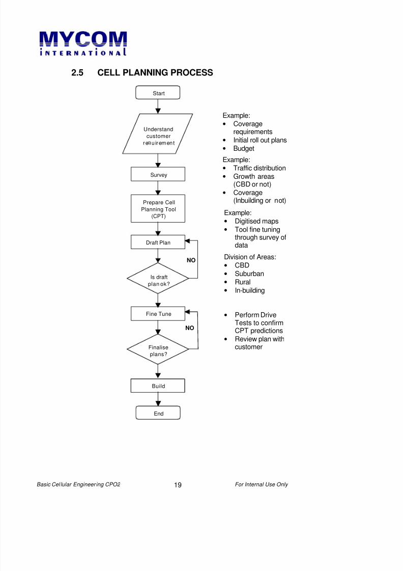
2.5 CELL PLANNING PROCESS

Start

Understandcustomer

re u irement

Survey

Prepare CellPlanning Tool

(CPT)

Draft Plan

Is draftplan ok?

Fine Tune

Finaliseplans?

Build

End

Example:• Coverage

requirements• Initial roll out plans• Budget

Example:• Traffic distribution• Growth areas

(CBD or not)• Coverage

(Inbuilding or not)Example:• Digitised maps• Tool fine tuning

through survey ofdata

Division of Areas:• CBD• Suburban• Rural• In-building

NO

NO

• Perform DriveTests to confirmCPT predictions

• Review plan withcustomer




2.6 CELL PLANNING CONSIDERATIONS

Some considerations are taken in cell planning. In the case of coverage versuscapacity, normally new networks need not concern itself with capacity as much

as coverage. Hence, high sites are normally built to maximise coverage (e.g. 50-70m high sites are very common).

However, as the network grows and become a more matured network, newconsiderations are taken. In this grown network, capacity is considered but thequality of service (QoS) is also important. Hence, there is a tradeoff betweenthese two factors. If more capacity is built, the quality will suffer.

END OF CHAPTER 2




CHAPTER 3

BASIC TELETRAFFIC THEORY

Objectives: This chapter describes the concept of traffic in a

cellular network. The description is from theErlang tables to dimensioning a cell.


• Explain the terms ‘traffic’ and ‘GoS’• Understand the concept of traffic• Use the Erlang B table to dimension the number of

channels needed in the system




3. BASIC TELETRAFFIC THEORY

3.1 INTRODUCTION

Traffic refers to usage of channels and is usually thought of as holding time pertime unit or the number of ‘call hours’ per hour for one or several channels. Trafficis measured in the unit Erlang (Er) and Erlang is defined as:-

The average number of channel simultaneously occupied during a defined period of time and it is dimensionless. For example, as shown in Figure 3-1.

Figure 3-1

Traffic from time period 0 to 10= (0+1+1+2+3+3+3+2+2+2)/10=1.9Er

The amount of traffic one cell can carry depends on the number of trafficchannels available and the acceptable probability that the system is congested(Grade of Service, GoS).

1

2

34

5

Time Unit

N o o f

c h a n n e l s




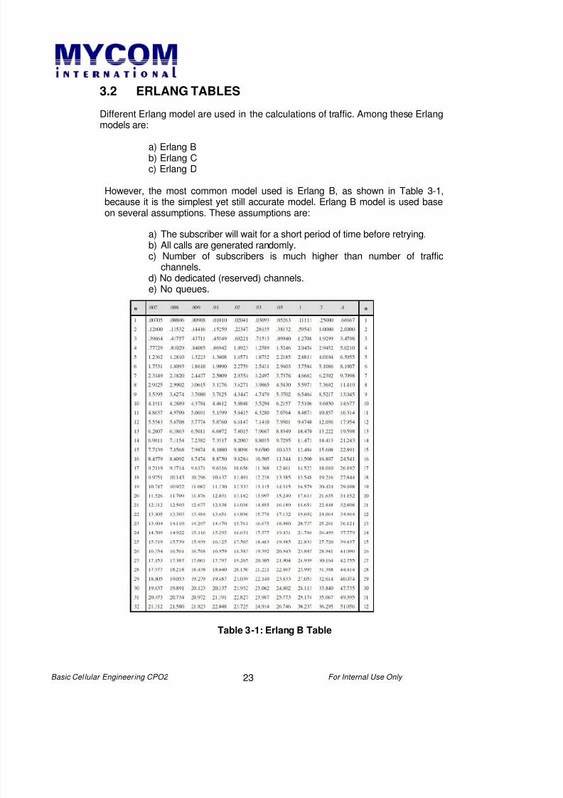
3.2 ERLANG TABLES

Different Erlang model are used in the calculations of traffic. Among these Erlangmodels are:

a) Erlang Bb) Erlang Cc) Erlang D

However, the most common model used is Erlang B, as shown in Table 3-1,because it is the simplest yet still accurate model. Erlang B model is used baseon several assumptions. These assumptions are:

a) The subscriber will wait for a short period of time before retrying.b) All calls are generated randomly.c) Number of subscribers is much higher than number of traffic

channels.

d) No dedicated (reserved) channels.e) No queues.

Table 3-1: Erlang B Table




3.3 TRAFFIC CONCEPTS

There are 3 different types of traffic. There are:-

a) Offered traffic (AO)This is the traffic offered to a group in accordance with a definedtheorectical description of the traffic case. It is consequently also ahypotectical quantity and it becomes only meaningful if it is referredto a specific theorectical model.

b) Carried traffic (AC)This is the traffic handled by a group. It can be measured and ismore practical to quote this traffic.

c) Loss traffic (AL)This is a portion of the traffic lost to an auxilliary route when theprimary route is occupied.

Generally,

AO = AC + AL and

AO = AC /(1-GoS)

3.4 DIMENSIONING A CELL

Dimensioning the network now implies using demographic data to determine thesizes of the cells. Dimensioning a whole network while maintaining a fixed cellsize means estimating the number of carriers needed in each cell. In addition,traffic is not constant since it varies between day and night, different days as wellas with a number of other factors. In GSM cellular system, the following are thetypical dimensions of a cell. For GoS of 2%, the number of offered traffic is:-

1 carrier = 2.9Er2 carrier = 8.2Er3 carrier = 14.03Er4 carrier = 21.04Er

It is important that the number of signalling channels (SDCCHs) is dimensionedas well, taking into account the estimated system behaviour in various parts of thenetwork. For example, cells bordering a different location area may have lots of

location updating and cells on a highway probably have many handovers. In orderto calculate the need for SDCCHs, the number of attempts for every procedurethat uses the SDCCH as well as the time that each procedure hold the SDCCHmust be taken into account. The procedures involved are location updating,periodic registration, IMSI attach/detach, call setup, SMS, facsimile andsupplementary services. The number of false accesses must also be estimated.This is typically quite a high number but still small compared to traffic.




3.5 SECTORED VS OMNI SITES

Omni sites are used in suburban to rural sites, which do not need capacity andwhen interference is not an issue. Meanwhile, sectored sites are used when

interference needs to be split and usually is used in suburban to urban and denseurban sites. The tradeoff between omni and sectored sites is the trunkingefficiency. This can be illustrated in an example given below.




Assume the task is to find the necessary number of traffic channels for one cell toserve subscribers with traffic of 33Er. The GoS during the busy hour is not toexceed 2%. By considering the above requirements and consulting Erlang’s B-table, 43 channels are found to be needed as shown in the Figure 3-2.

Figure 3-2: Part of Erlang B’s Table for 43 channels

giving the offered traffic (Er) as a function of the GoS

(%)

Assume five cells are designed to cover the same area as the single cell. Thesefive cells must handle the same amount of traffic as the cell above, 33Er.Acceptable GoS is still 2%. First, the total traffic is divided among the cells (Table3-2). Traffic distribution over several cells results in a need for more channelsthan if all traffic had been concentrated in one cell.

This illustrates the fact that it is more efficient to use many channels in a largercell than vice versa. To calculate the channel utilization, the traffic offered isreduced by the GoS of 2% (yielding the carried traffic) and dividing that value bythe number of channels (yielding the channel utilization).

With 43 channels (as in the previous single cell example), the channel utilizationis 33.083/ 43 = 77%, i.e., each channel is used approximately 77% of the time.However, by splitting this cell into smaller cells, more traffic channels are requiredhence the channel utilization decreases.

Table 3-2: A certain amount of traffic is distributed over several cells

END OF CHAPTER 3




CHAPTER 4

BASIC ANTENNA THEORY

Objectives: This chapter explains the basic antenna studiesfrom the type of radiation to the type of antennas

used as well as some of the antennas’specifications.


• Understand the concept of the antenna radiation• Describe some of the antenna types as well as the

specifications needed




4. BASIC ANTENNA THEORY

4.1 INTRODUCTION

An antenna is a radiating element that is fed with an electromagnetic energy.Oscillating charges on a transmitting antenna typically generate ultra highfrequency radio waves. Each antenna has a unique radiation pattern. This patterncan be represented graphically by plotting the received, time-averaged power as afunction of the angle that is with respect to the direction of maximum power in alog-polar diagram. The pattern is a representative of the antenna’s performance ina test environment. However, it only applies to the free-space environment in whichthe test measurement takes place. Upon installation, the pattern becomes morecomplex due to factors affecting propagation in the reality. Thus, the realeffectiveness of any antenna is measured in the field.

4.2 ISOTROPIC RADIATION

An isotropic antenna is a completely non-directional antenna that radiates equallyin all directions. Since all practical antennas exhibit some degree of directivity, theisotropic antenna exists only as a mathematical concept. The isotropic antennacan be used as a reference to specify the gain of a practical antenna. The gain ofan antenna referenced isotropically is the ratio between the power required in thepractical antenna and the power required in an isotropic antenna to achieve thesame field strength in the desired direction of the measured practical antenna.

Isotropic radiation only exists in an ideal situation. In practice, radiation does notpropagate equally in all direction but favouring one direction over another.

Figure 4-1

Figure 4-1 above shows an isotropic source, which is an imaginary origin pointwhere energy is being radiated equally in all spherical direction.




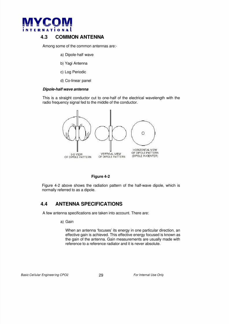
4.3 COMMON ANTENNA

Among some of the common antennas are:-

a) Dipole-half waveb) Yagi Antenna

c) Log Periodic

d) Co-linear panel

Dipole-half wave antenna

This is a straight conductor cut to one-half of the electrical wavelength with theradio frequency signal fed to the middle of the conductor.

Figure 4-2

Figure 4-2 above shows the radiation pattern of the half-wave dipole, which isnormally referred to as a dipole.

4.4 ANTENNA SPECIFICATIONS

A few antenna specifications are taken into account. There are:

a) Gain

When an antenna ‘focuses’ its energy in one particular direction, aneffective gain is achieved. This effective energy focused is known asthe gain of the antenna. Gain measurements are usually made withreference to a reference radiator and it is never absolute.




The directive gain in relation to an isotropic antenna is expressed inunits of dBi and the directive gain in relation to a dipole is expressedin units of dBd. For a dipole and an isotropic antenna with the sameinput power, the energy is more concentrated in certain directions bythe dipole.

Generally,

dBi = dBd + 2.15dB

Cellular antennae specifications are usually quoted in dBi.

Figure 4-3

Figure 4-3 above shows the differences in gain between theisotropic, dipole and practical antenna. The vertical pattern for thepractical antenna is that of a directional antenna.

The gain of an antenna is related to its effective aperture accordingto the formula below,

Ae = Gλ2 /4π

Thus, Ae ∝ λ. This means that the greater the affective aperture, thegreater the gain of the antenna and the size of an antenna isinversely proportional to the frequency of operation.




An antenna and the cable are passive elements whereas the power amplifier is anactive element. The reason that the output power can be higher than the inputpower is because of the directive gain of the antenna as shown in Figure 4-4.

b) Beamwidth

Beamwidth is defined as the angular separation between two –3dBpoints on the field strength radiation pattern of an antenna. It can bespecified horizontally and vertically. The beamwidth specification isuseful because it gives us an idea of where most of the useful

antenna energy is pointing. This specification can be found from thepolar plots provided by the manufacturer. The typical values are 90°,65° and 120°.

Power Amplifier

10W

3dB cable loss

6dBantenna

gain

How much power radiating?

PASSIVE

ACTIVE

20W

Figure 4-4

Figure 4-5




Figure 4-5 shows the definition of beamwidth. Both the horizontal and verticalbeamwidths are found using the 3dB down points, alternatively referred to as half-power points.

Figure 4-6 below shows the vertical and hozintal antenna pattern for a ‘real’

antenna.

Figure 4-6




c) Antenna Data Sheet

When choosing an antenna for a specific application, themanufacturer’s data sheet must be consulted. The data sheetcontains information including antenna gain, beamwidth (vertical and

horizontal) and graphs showing the vertical and horizontal patterns.

Figure 4-7

Figure 4-7 is an example of an antenna data sheet, where the patterns of thebeamwidths are also shown.

d) Front to back ratio

This is a ratio of the front gain to the back gain specified in dBs.The front to back ratio is a useful information to have when

considering an antenna type for a specific design. The typical valueis between 25-30 Bs. The larger the value, the better the separationbetween the front and back ratio radiation lobe.

e) Polarisation type




There are 2 types of polarisation namely:-

i) Uni-polarThis antenna only has elements radiating in one phase. It isused when spatial diversity is employed.

ii) Dual polarThis antenna has elements radiating in two phase either in 90° of each other or 45° of each other. It is used when polarisationdiversity is used.

f) Beam tilt angle

There are 2 types of beam tilt namely:-

i) Mechanical

In mechanical tilting, the horizontal beamwidth increases withthe rising of the downtilt angle. The resulting gain reductiondepends on the azimuth directions.

Figure 4-8

Figure 4-8 above shows the mechanical beam tilt of an antenna.

ii) Electrical




This type of beam tilt has a constant downtilt angle over thewhole azimuth range. The horizontal beamwidth isindependent of the down tilt angle.

Figure 4-9

Both the diagrams in Figure 4-9 above show the effect of horizontal radiationpattern at various tilt angles. Other specifications that are taken into account are:-

a) Other auxilliary specification

b) Power handlingc) Connector typed) Dimensions and weighte) VSWR/Return loss specificationf) Impedance

END OF CHAPTER 4




CHAPTER 5

COMMON RF ANCILLIARIES

Objectives: This chapter explains on the general equipmentused in antenna installations such as thecouplers, isolators, duplexers and many more.


• Describe the concept of the equipment used for RFnetworks

5. COMMON RF ANCILLIARIES




5.1 EQUIPMENT

The concepts involved in dealing with the equipment are:-

a) Insertion lossLosses that are due when two ports are connected together,typcically connectors or equipment ports.

b) Impedance matching/VSWRReflections cause standing waves of voltage and current on atranmission line if it is not terminated with the characteristicimpedance, Zo.

The characteristic impedance is defined as below:

Zo = [138/ √K] • [log (b/a)]

Where a = inner conductor diameterb = inner diameter of outer conductorK = relative dielectric constant = 1 in vacuum

Standing waves increase line losses, mostly due to higher currents.They are also indicative of mismatches that result in losses and candegrade filter performance. The Standing Wave Ratio (SWR) orVoltage Standing Wave Ratio (VSWR) is defined as:

VSWR = [1 +ρ] / [1 - ρ]

Where ρ = reflection coefficient= [ZL – Zo] / [ZL + Zo] and ZL is complex

Also,

ρ = [VSWR – 1] / [VSWR + 1]

For purely resistive loads only,

VSWR = RL / Zo (RL ≥ Zo) or

VSWR = Zo / RL (RL ≤ Zo)

c) Bandwidth




Bandwidth is the term used to describe the amount of frequencyrange allocated to one application. The bandwidth given to anapplication depends on the amount of available frequency spectrum.The amount of bandwidth available is an important factor indetermining the capacity of a mobile system, that is the number ofcalls, which can be handled.

d) Power ratingThe power rating is an important figure that decribes the optimumand maximum power range that a passive device can handle beforereaching critical breakdown of the device.

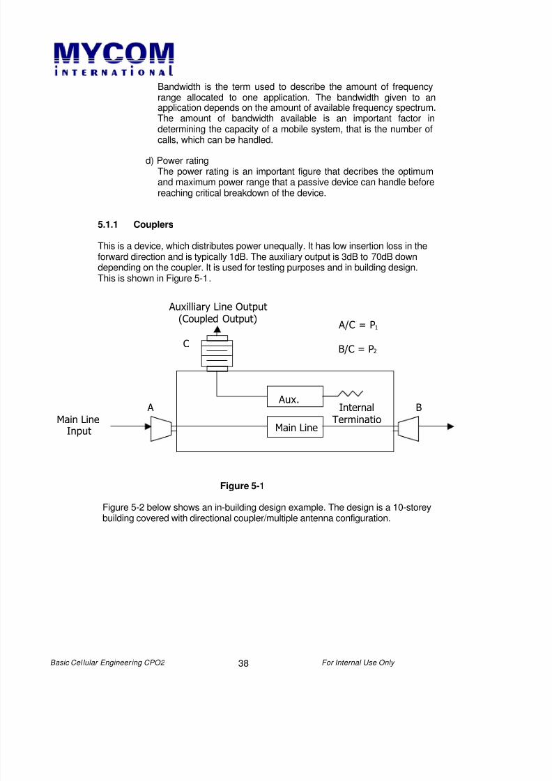
5.1.1 Couplers

This is a device, which distributes power unequally. It has low insertion loss in theforward direction and is typically 1dB. The auxiliary output is 3dB to 70dB downdepending on the coupler. It is used for testing purposes and in building design.This is shown in Figure 5-1.

Figure 5-1

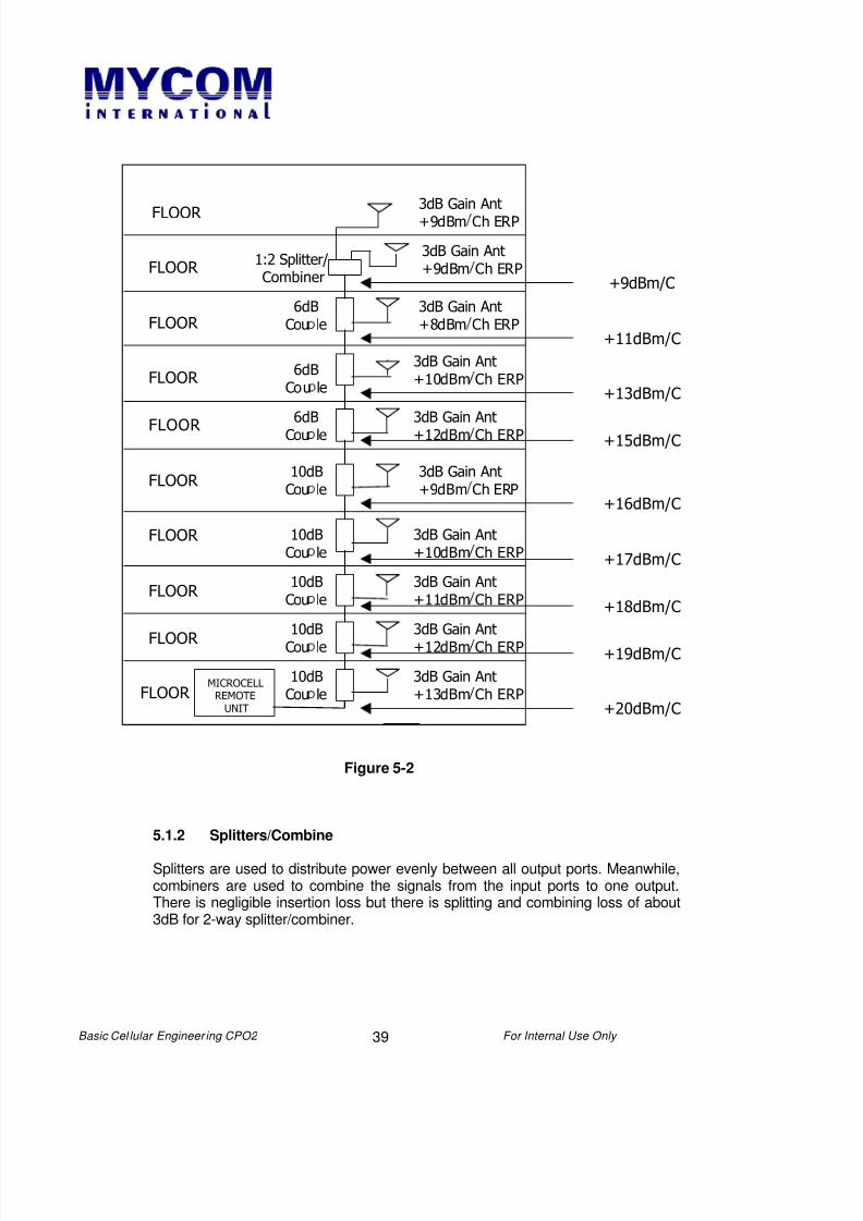
Figure 5-2 below shows an in-building design example. The design is a 10-storeybuilding covered with directional coupler/multiple antenna configuration.

Main Line

Aux.

Main LineInput

Auxilliary Line Output(Coupled Output)

C

A BInternalTerminatio

A/C = P1

B/C = P2




Figure 5-2

5.1.2 Splitters/Combine

Splitters are used to distribute power evenly between all output ports. Meanwhile,combiners are used to combine the signals from the input ports to one output.There is negligible insertion loss but there is splitting and combining loss of about3dB for 2-way splitter/combiner.

MICROCELLREMOTE

UNIT

FLOOR

FLOOR

FLOOR

FLOOR

FLOOR

FLOOR

FLOOR

FLOOR

FLOOR

FLOOR

+20dBm/C

+19dBm/C

+17dBm/C

+18dBm/C

+16dBm/C

+15dBm/C

+13dBm/C

+11dBm/C

+9dBm/C

3dB Gain Ant

+13dBm Ch ERP

3dB Gain Ant

+12dBm Ch ERP

3dB Gain Ant

+11dBm Ch ERP

3dB Gain Ant

+10dBm Ch ERP

3dB Gain Ant

+9dBm Ch ERP

3dB Gain Ant

+12dBm Ch ERP

3dB Gain Ant

+10dBm Ch ERP

3dB Gain Ant

+8dBm Ch ERP

3dB Gain Ant

+9dBm Ch ERP

3dB Gain Ant

+9dBm Ch ERP

10dB

Cou le

10dB

Cou le

10dB

Cou le

10dB

Cou le

10dB

Cou le

6dB

Cou le

6dB

Cou le

6dB

Cou le

1:2 Splitter/Combiner




5.1.3 Filters

Bandpass filters allow signals within a band of frequency to pass and attenuate allsignals outside the band. An example is the GSM bandpass filter. Combline filtersare used when sharp roll-off or attenuation is required. Typically, it is used todifferentiate TX and RX band. This is illustrated in Figure 5-3.

Figure 5-3

5.1.4 Duplexers

Duplexer is used to separate transmit and receive signals by using 2 comblinefilters. It allows for transmit and receive from a single antenna as shown in Figure5-4.

Frequency in MHz

PD5182 RESPONSE CURVE (896-902) Attenuation in dB

AntennaTx/Rx

Figure 5-4

DUPLEXER

Tx

Rx



5.1.5 Isolators

Isolator is a directional device, which protects the equipment (typically transmitters)from damage by any power flowing in reverse. Isolation also prevents inter-modulation by preventing any unwanted signals from entering back into the activedevices (i.e. high isolation between transmitters).

5.1.6 Cables/Connectors

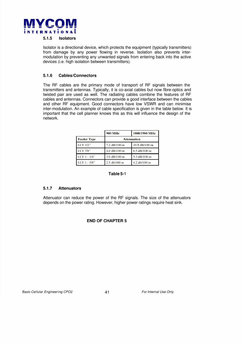
The RF cables are the primary mode of transport of RF signals between thetransmitters and antennas. Typically, it is co-axial cables but now fibre-optics andtwisted pair are used as well. The radiating cables combine the features of RFcables and antennas. Connectors can provide a good interface between the cablesand other RF equipment. Good connectors have low VSWR and can minimiseinter-modulation. An example of cable specification is given in the table below. It isimportant that the cell planner knows this as this will influence the design of thenetwork.

Table 5-1

5.1.7 Attenuators

Attenuator can reduce the power of the RF signals. The size of the attenuatorsdepends on the power rating. However, higher power ratings require heat sink.

END OF CHAPTER 5

basic cellular radio engineering document

Documents