basic backward trajectory to gis instructions
TRANSCRIPT
1 of 22
Basic Backward Trajectory to GIS Instructions
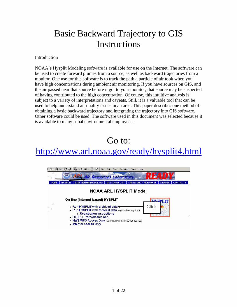
Introduction NOAA’s Hysplit Modeling software is available for use on the Internet. The software can be used to create forward plumes from a source, as well as backward trajectories from a monitor. One use for this software is to track the path a particle of air took when you have high concentrations during ambient air monitoring. If you have sources on GIS, and the air passed near that source before it got to your monitor, that source may be suspected of having contributed to the high concentration. Of course, this intuitive analysis is subject to a variety of interpretations and caveats. Still, it is a valuable tool that can be used to help understand air quality issues in an area. This paper describes one method of obtaining a basic backward trajectory and integrating the trajectory into GIS software. Other software could be used. The software used in this document was selected because it is available to many tribal environmental employees.
Go to: http://www.arl.noaa.gov/ready/hysplit4.html
Click
2 of 22
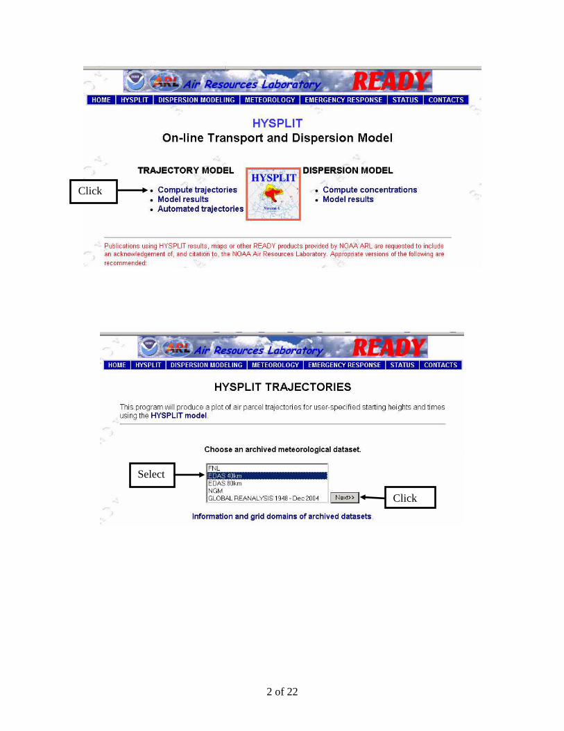
Click
Select
Click
3 of 22
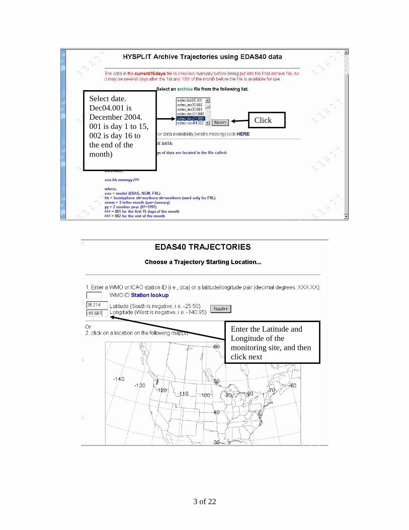
Select date. Dec04.001 is December 2004. 001 is day 1 to 15, 002 is day 16 to the end of the month)
Enter the Latitude and Longitude of the monitoring site, and then click next
Click
4 of 22
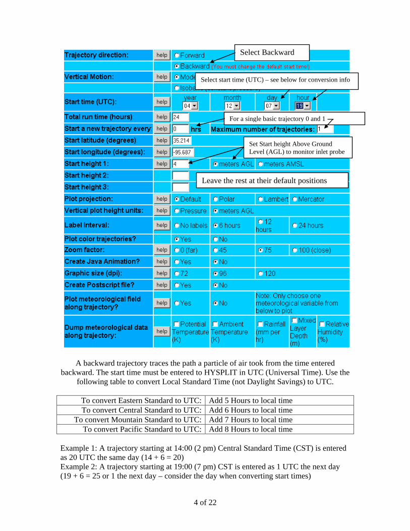
A backward trajectory traces the path a particle of air took from the time entered backward. The start time must be entered to HYSPLIT in UTC (Universal Time). Use the
following table to convert Local Standard Time (not Daylight Savings) to UTC.
To convert Eastern Standard to UTC: Add 5 Hours to local time To convert Central Standard to UTC: Add 6 Hours to local time
To convert Mountain Standard to UTC: Add 7 Hours to local time To convert Pacific Standard to UTC: Add 8 Hours to local time
Example 1: A trajectory starting at 14:00 (2 pm) Central Standard Time (CST) is entered as 20 UTC the same day (14 + 6 = 20) Example 2: A trajectory starting at 19:00 (7 pm) CST is entered as 1 UTC the next day (19 + 6 = 25 or 1 the next day – consider the day when converting start times)
Select Backward
Select start time (UTC) – see below for conversion info
For a single basic trajectory 0 and 1
Set Start height Above Ground Level (AGL) to monitor inlet probe
Leave the rest at their default positions
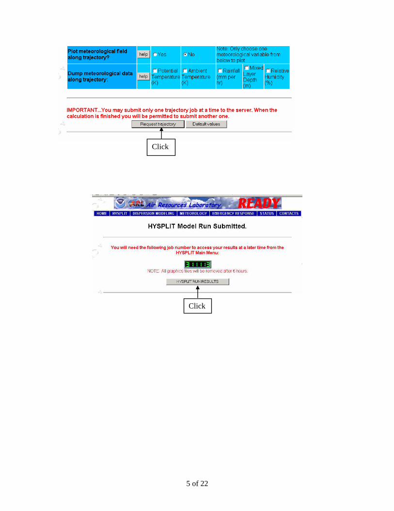
5 of 22
Click
Click
6 of 22
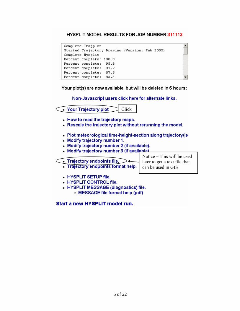
Click
Notice – This will be used later to get a text file that can be used in GIS
7 of 22
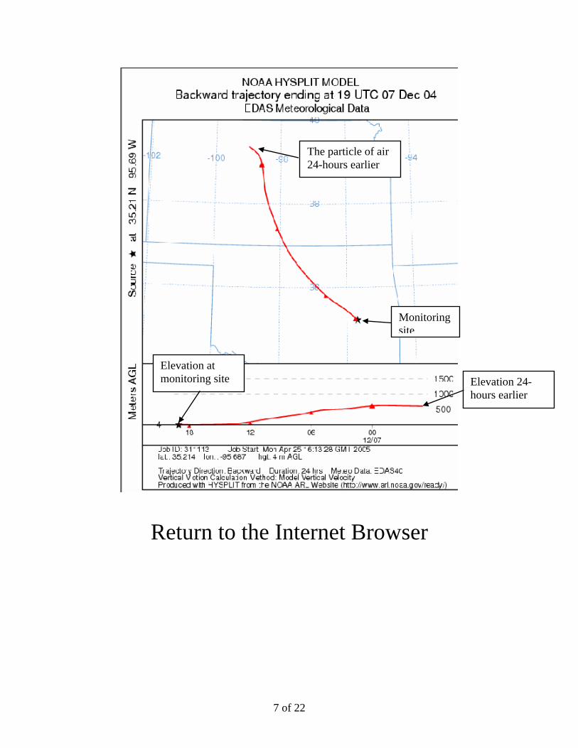
Return to the Internet Browser
Monitoring site
The particle of air 24-hours earlier
Elevation at monitoring site Elevation 24-
hours earlier
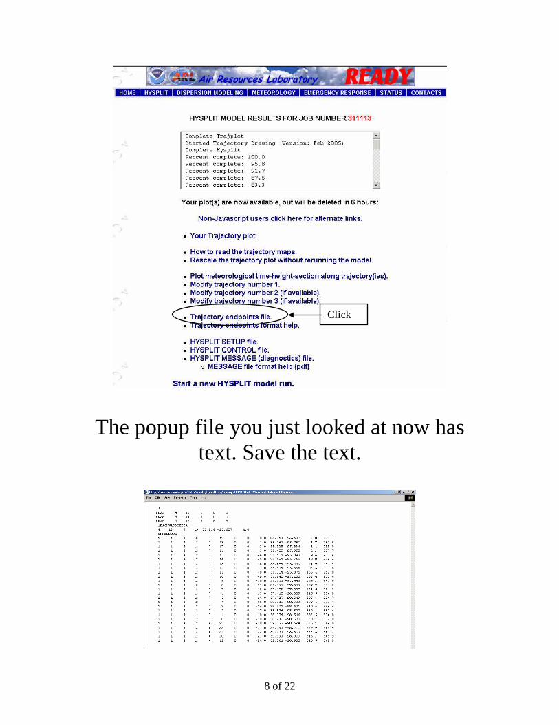
8 of 22
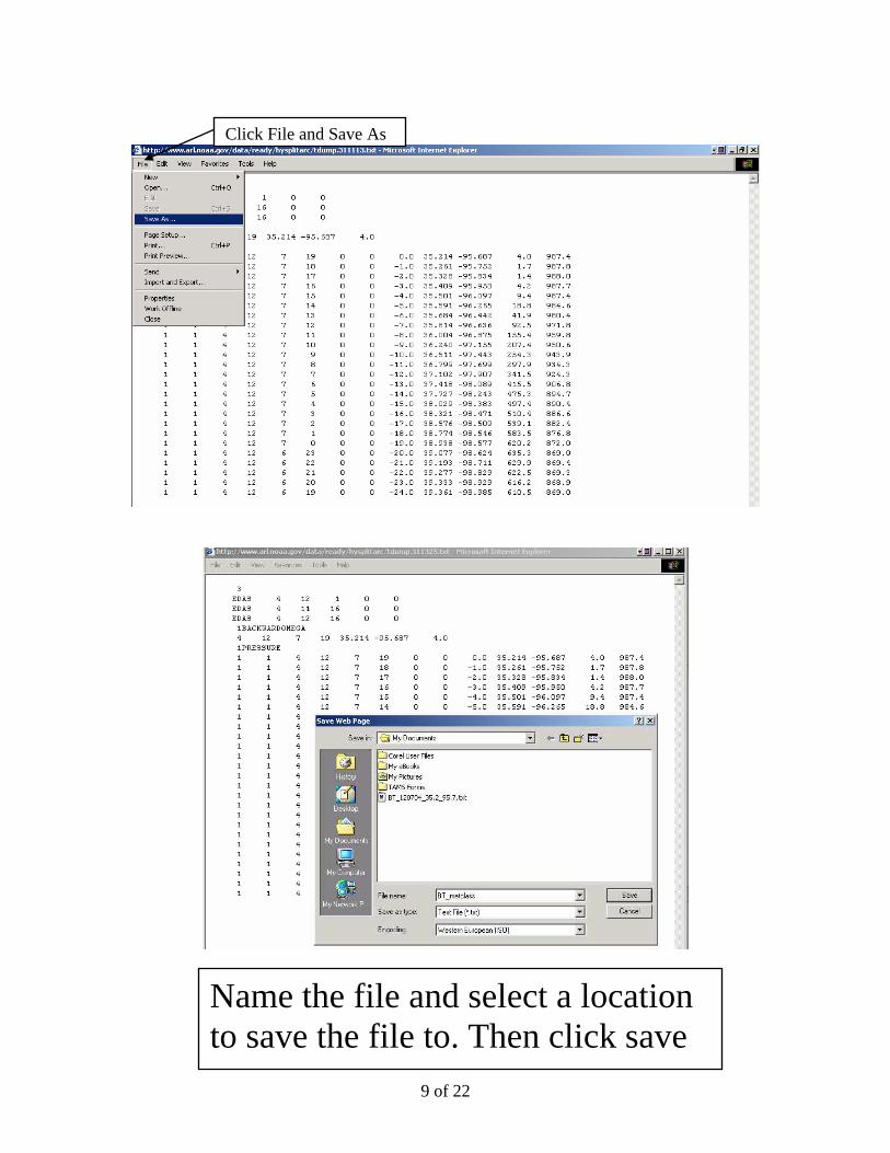
The popup file you just looked at now has text. Save the text.
Click
9 of 22
Name the file and select a location to save the file to. Then click save
Click File and Save As
10 of 22
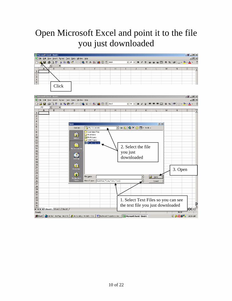
Open Microsoft Excel and point it to the file you just downloaded
Click
1. Select Text Files so you can see the text file you just downloaded
2. Select the file you just downloaded
3. Open
11 of 22
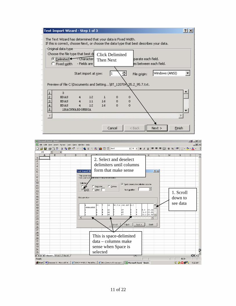
Click Delimited Then Next
1. Scroll down to see data
2. Select and deselect delimiters until columns form that make sense
This is space-delimited data – columns make sense when Space is selected
12 of 22
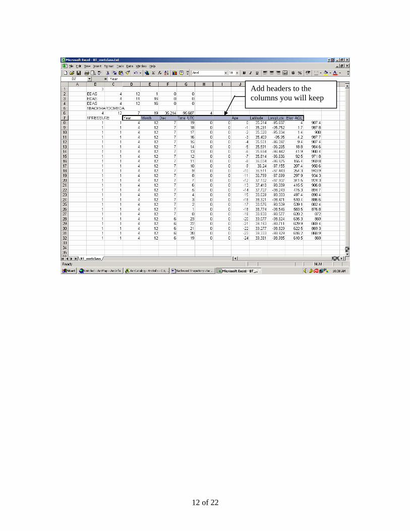
Add headers to the columns you will keep
13 of 22
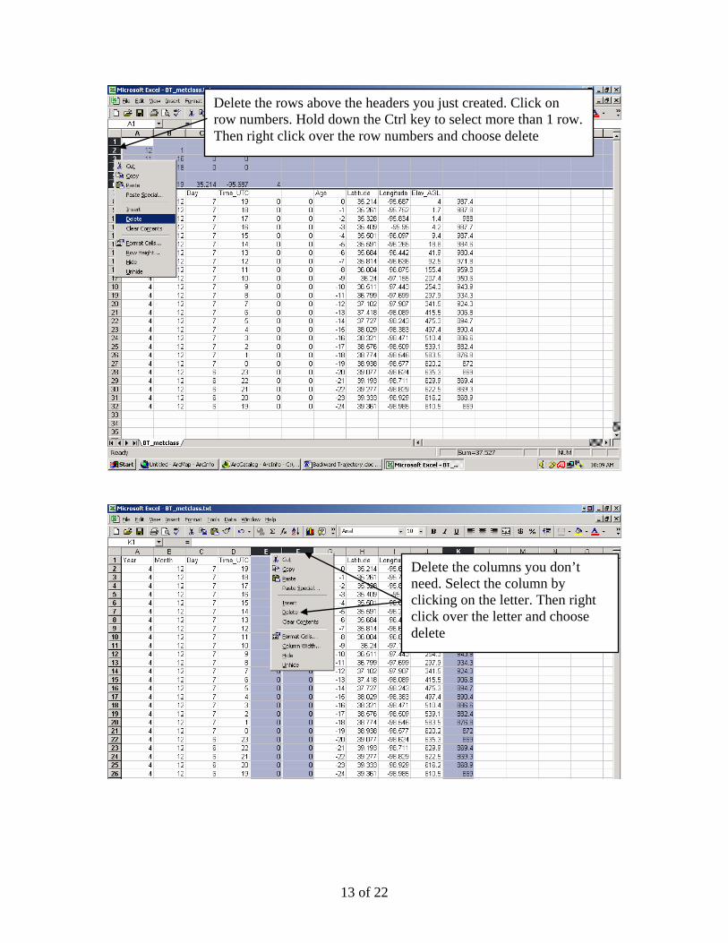
Delete the rows above the headers you just created. Click on row numbers. Hold down the Ctrl key to select more than 1 row. Then right click over the row numbers and choose delete
Delete the columns you don’t need. Select the column by clicking on the letter. Then right click over the letter and choose delete
14 of 22
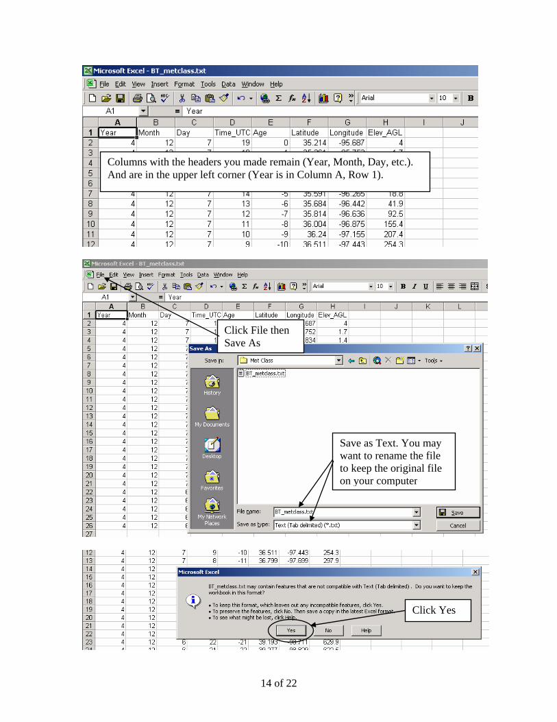
Columns with the headers you made remain (Year, Month, Day, etc.). And are in the upper left corner (Year is in Column A, Row 1).
Click File then Save As
Save as Text. You may want to rename the file to keep the original file on your computer
Click Yes
15 of 22
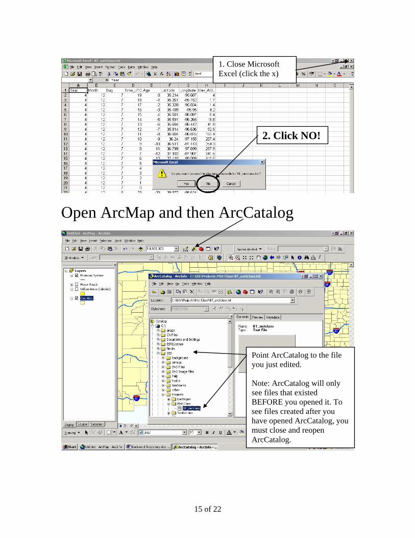
Open ArcMap and then ArcCatalog
1. Close Microsoft Excel (click the x)
2. Click NO!
Point ArcCatalog to the file you just edited. Note: ArcCatalog will only see files that existed BEFORE you opened it. To see files created after you have opened ArcCatalog, you must close and reopen ArcCatalog.
16 of 22
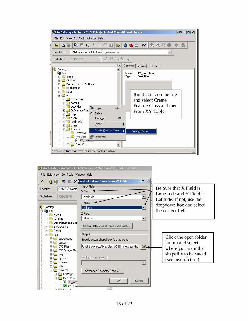
Right Click on the file and select Create Feature Class and then From XY Table
Be Sure that X Field is Longitude and Y Field is Latitude. If not, use the dropdown box and select the correct field
Click the open folder button and select where you want the shapefile to be saved (see next picture)
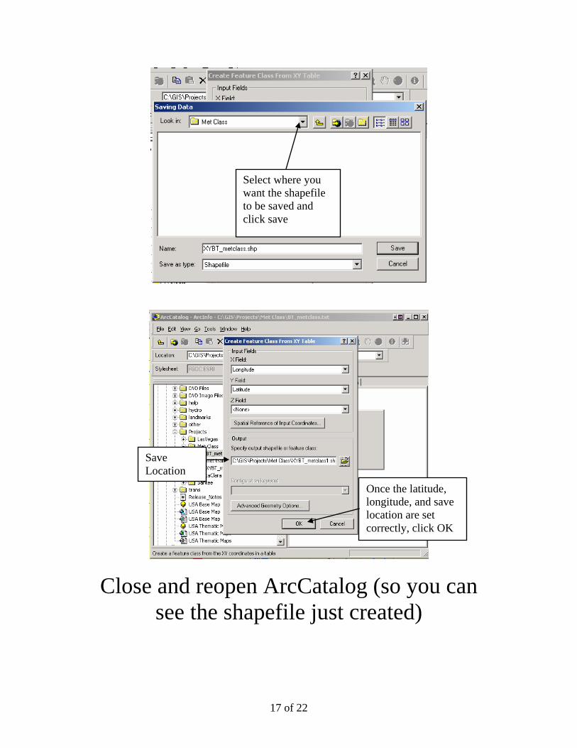
17 of 22
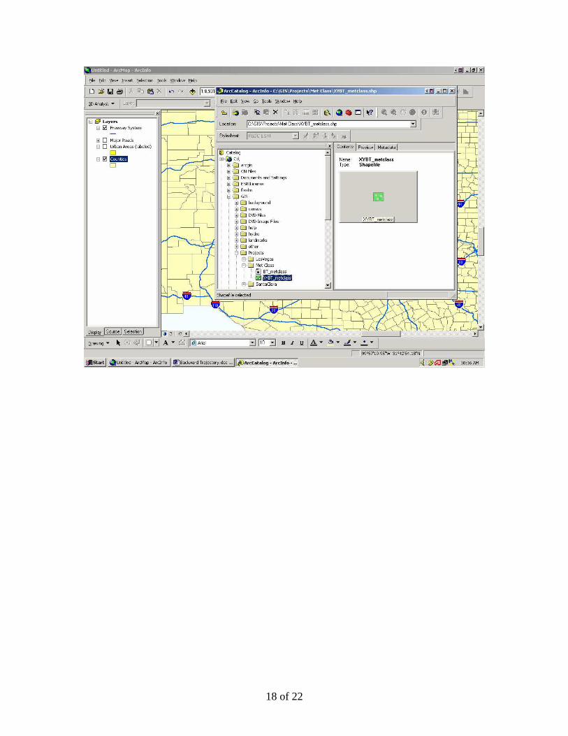
Close and reopen ArcCatalog (so you can see the shapefile just created)
Select where you want the shapefile to be saved and click save
Once the latitude, longitude, and save location are set correctly, click OK
Save Location
18 of 22
19 of 22
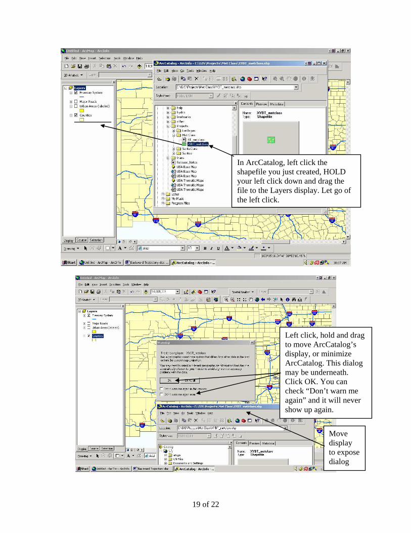
In ArcCatalog, left click the shapefile you just created, HOLD your left click down and drag the file to the Layers display. Let go of the left click.
Left click, hold and drag to move ArcCatalog’s display, or minimize ArcCatalog. This dialog may be underneath. Click OK. You can check “Don’t warn me again” and it will never show up again.
Move display to expose dialog
20 of 22
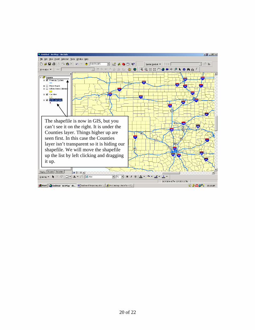
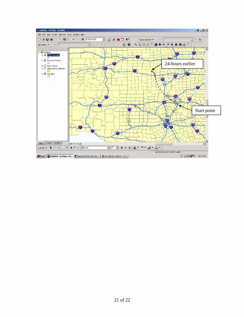
The shapefile is now in GIS, but you can’t see it on the right. It is under the Counties layer. Things higher up are seen first. In this case the Counties layer isn’t transparent so it is hiding our shapefile. We will move the shapefile up the list by left clicking and dragging it up.
21 of 22
Start point
24-hours earlier
22 of 22
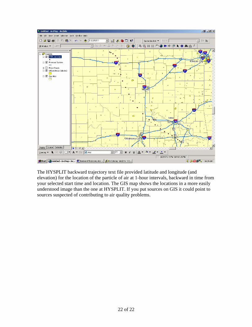
The HYSPLIT backward trajectory text file provided latitude and longitude (and elevation) for the location of the particle of air at 1-hour intervals, backward in time from your selected start time and location. The GIS map shows the locations in a more easily understood image than the one at HYSPLIT. If you put sources on GIS it could point to sources suspected of contributing to air quality problems.