ARCH/GARCH Models

1

Risk Management

Risk: the quantifiable likelihood of loss or less-than-expected

returns.

In recent decades the field of financial risk management has

undergone explosive development.

Risk management has been described as “one of the most

important innovations of the 20th century”.

But risk management is not something new.

2

Risk Management

José (Joseph) De La Vega was a

Jewish merchant and poet residing

in 17th century Amsterdam.

There was a discussion between a

lawyer, a trader and a philosopher

in his book Confusion of

Confusions.

Their discussion contains what we

now recognize as European options

and a description of their use for

risk management.

3

Risk Management

There are three major risk types:

market risk: the risk of a change in the value of a financial

position due to changes in the value of the underlying assets.

credit risk: the risk of not receiving promised repayments

on outstanding investments.

operational risk: the risk of losses resulting from inadequate

or failed internal processes, people and systems, or from

external events.

4

Risk Management VaR (Value at Risk), introduced by JPMorgan in the 1980s, is

probably the most widely used risk measure in financial

institutions.

5

Risk Management Given some confidence level 𝛼 ∈ 0,1 . The VaR of our

portfolio at the confidence level α is given by the smallest

value 𝑙 such that the probability that the loss 𝐿 exceeds 𝑙 is

no larger than 𝛼.

6

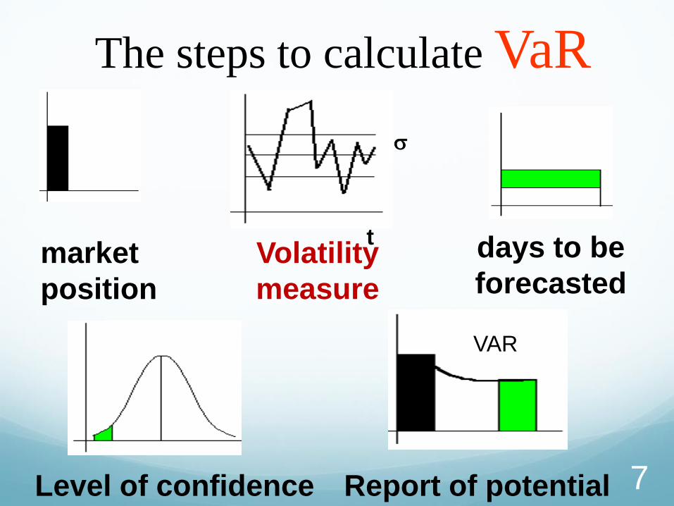
The steps to calculate VaR

market

position

s

t Volatility

measure

days to be

forecasted

Report of potential

loss

VAR

Level of confidence 7

The success of VaR

Is a result of the method used to estimate the

risk

The certainty of the report depends upon the

type of model used to compute the volatility on which these forecast is based

8

Volatility

9

Volatility

10

11

Modeling Volatility with

ARCH & GARCH

In 1982, Robert Engle developed the autoregressive

conditional heteroskedasticity (ARCH) models to model the

time-varying volatility often observed in economical time

series data. For this contribution, he won the 2003 Nobel Prize

in Economics (*Clive Granger shared the prize for co-

integration http://www.nobelprize.org/nobel_prizes/economic-sciences/laureates/2003/press.html).

ARCH models assume the variance of the current error

term or innovation to be a function of the actual sizes of the

previous time periods' error terms: often the variance is related

to the squares of the previous innovations.

In 1986, his doctoral student Tim Bollerslev developed the

generalized ARCH models abbreviated as GARCH.

12

Volatility of Merval Index modelling

whith Garch (1,1)

0

2

4

6

8

10

12

14

16

12/0

1/1

994

03/1

0/1

995

06/2

2/1

995

09/2

8/1

995

01/1

0/1

996

04/1

8/1

996

07/3

0/1

996

11/0

5/1

996

02/1

3/1

997

05/2

6/1

997

09/0

4/1

997

12/1

1/1

997

03/2

3/1

998

07/0

8/1

998

10/2

1/1

998

02/0

1/1

999

05/1

2/1

999

08/2

5/1

999

12/0

2/1

999

03/2

1/2

000

07/0

6/2

000

10/1

3/2

00013

Time series

14

Time series-ARCH (*Note, Zt can be other white noise, no need to be Gaussian)

Let 𝑍𝑡 be N(0,1). The process 𝑋𝑡 is an ARCH(q) process if it

is stationary and if it satisfies, for all 𝑡 and some strictly

positive-valued process 𝜎𝑡, the equations

𝑋𝑡 = 𝜎𝑡𝑍𝑡

𝜎𝑡2 = 𝛼0 + 𝛼𝑖𝑋𝑡−𝑖

2

𝑞

𝑖=1

Where 𝛼0 > 0 and 𝛼𝑖 ≥ 0, 𝑖 = 1, . . . , 𝑞.

Note: 𝑿𝒕 is usually the error term in a time series

regression model! 15

Time series-ARCH

ARCH(q) has some useful properties. For simplicity, we will show them

in ARCH(1).

Without loss of generality, let a ARCH(1) process be represented by

𝑋𝑡 = 𝑍𝑡 𝛼0 + 𝛼1𝑋𝑡−12

Conditional Mean

𝐸 𝑋𝑡 𝐼𝑡−1 = 𝐸 𝑍𝑡 𝛼0 + 𝛼1𝑋𝑡−12 𝐼𝑡−1 = 𝐸 𝑍𝑡 𝐼𝑡−1 𝛼0 + 𝛼1𝑋𝑡−1

2 = 0

Unconditional Mean

𝐸 𝑋𝑡 = 𝐸 𝑍𝑡 𝛼0 + 𝛼1𝑋𝑡−12 = 𝐸 𝑍𝑡 𝐸 𝛼0 + 𝛼1𝑋𝑡−1

2 = 0

So 𝑋𝑡 have mean zero 16

Time series-ARCH

17

Time series-ARCH

𝑋𝑡 have unconditional variance given by 𝑉𝑎𝑟 𝑋𝑡 =𝛼0

1−𝛼1

Proof 1 (use the law of total variance):

𝑉𝑎𝑟 𝑋𝑡 = 𝐸 𝑉𝑎𝑟 𝑋𝑡 𝐼𝑡−1 + 𝑉𝑎𝑟 𝐸 𝑋𝑡 𝐼𝑡−1

= 𝐸 𝛼0 + 𝛼1𝑋𝑡−12 + 𝑉𝑎𝑟 0

= 𝛼0 + 𝛼1𝐸 𝑋𝑡−12

= 𝛼0 + 𝛼1𝑉𝑎𝑟(𝑋𝑡−1)

Because it is stationary, 𝑉𝑎𝑟 𝑋𝑡 = 𝑉𝑎𝑟(𝑋𝑡−1).

So 𝑉𝑎𝑟 𝑋𝑡 =𝛼0

1−𝛼1.

18

Time series-ARCH

Proof 2:

Lemma: Law of Iterated Expectations

Let Ω1 and Ω2 be two sets of random variables such that

Ω1 ⊆ Ω2. Let 𝑌 be a scalar random variable. Then

𝐸 𝑌 Ω1 = 𝐸 𝐸 𝑌 Ω2 Ω1

𝑉𝑎𝑟 𝑋𝑡 𝐼𝑡−2 = 𝐸 𝑋𝑡2 𝐼𝑡−2 = 𝐸 𝐸 𝑋𝑡

2 𝐼𝑡−1 𝐼𝑡−2

= 𝛼0 + 𝛼1𝐸 𝑋𝑡−12 𝐼𝑡−2 = 𝛼0 + 𝛼0𝛼1 + 𝛼1

2𝑋𝑡−22

𝑉𝑎𝑟 𝑋𝑡 𝐼𝑡−3 = 𝛼0 + 𝛼0𝛼1 + 𝛼0𝛼12 + 𝛼1

3𝑋𝑡−32

…

𝑉𝑎𝑟 𝑋𝑡 = 𝐸 𝑋𝑡2 = 𝐸 𝐸 …𝐸 𝑋𝑡

2 𝐼𝑡−1 … 𝐼1= 𝛼0 1 + ⋯+ 𝛼1

𝑡−1 + 𝛼1𝑡𝑋0

2

Since𝛼1 < 1, as 𝑡 → ∞, 𝑉𝑎𝑟 𝑋𝑡 =𝛼0

1−𝛼1

19

Time series-ARCH

The unconditional distribution of Xt is leptokurtic, it is easy

to show.

𝐾𝑢𝑟𝑡 𝑋𝑡 =𝐸(𝑋𝑡

4)

[𝐸(𝑋𝑡2)]2

= 31 − 𝛼1

2

1 − 3𝛼12 > 3

Proof:

𝐸 𝑋𝑡4 = 𝐸 𝐸 𝑋𝑡

4 𝐼𝑡−1 = 𝐸 𝜎𝑡4𝐸 𝑍𝑡

4 𝐼𝑡−1

= 𝐸 𝑍𝑡4 𝐸 𝛼0 + 𝛼1𝑋𝑡−1

2 2

= 3(𝛼02 + 2𝛼0𝛼1𝐸 𝑋𝑡−1

2 + 𝛼12𝐸(𝑋𝑡−1

4 ))

So 𝐸 𝑋𝑡4 = 3

𝛼02

1−𝛼1

1+𝛼1

1−3𝛼12. Also, 𝐸 𝑋𝑡

2 =𝛼0

1−𝛼1

𝐾𝑢𝑟𝑡 𝑋𝑡 =𝐸(𝑋𝑡

4)

[𝐸(𝑋𝑡2)]2

= 31 − 𝛼1

2

1 − 3𝛼12

20

fatter

tails

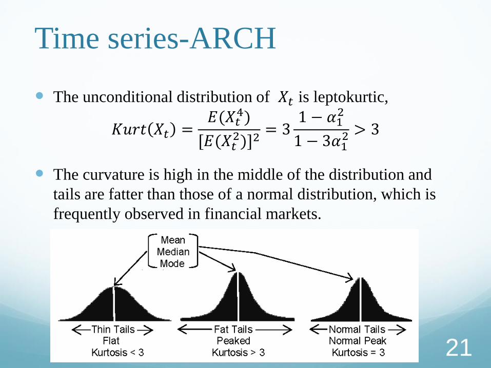
Time series-ARCH

The unconditional distribution of 𝑋𝑡 is leptokurtic,

𝐾𝑢𝑟𝑡 𝑋𝑡 =𝐸(𝑋𝑡

4)

[𝐸(𝑋𝑡2)]2

= 31 − 𝛼1

2

1 − 3𝛼12 > 3

The curvature is high in the middle of the distribution and

tails are fatter than those of a normal distribution, which is

frequently observed in financial markets.

21

Time series-ARCH For ARCH(1), we can rewrite it as

𝑋𝑡2 = 𝜎𝑡

2𝑍𝑡2 = 𝛼0 + 𝛼1𝑋𝑡−1

2 + 𝑉𝑡

where

𝑉𝑡 = 𝜎𝑡2 𝑍𝑡

2 − 1

𝐸(𝑋𝑡4) is finite, then it is an AR(1) process for

𝑋𝑡2.

Another perspective: 𝐸(𝑋𝑡2 𝐼𝑡−1 = 𝛼0 + 𝛼1𝑋𝑡−1

2

The above is simply the optimal forecast of

𝑋𝑡2 if it follows an AR(1) process

22

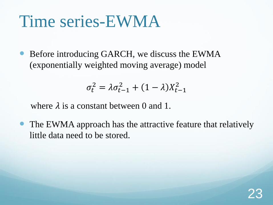
Time series-EWMA

Before introducing GARCH, we discuss the EWMA

(exponentially weighted moving average) model

𝜎𝑡2 = 𝜆𝜎𝑡−1

2 + 1 − 𝜆 𝑋𝑡−12

where 𝜆 is a constant between 0 and 1.

The EWMA approach has the attractive feature that relatively

little data need to be stored.

23

Time series-EWMA

We substitute for 𝜎𝑡−12 ,and then keep doing it for 𝑚 steps

𝜎𝑡2 = 1 − 𝜆 𝜆𝑖−1

𝑚

𝑖=1

𝑋𝑡−𝑖2 + 𝜆𝑚𝜎𝑡−𝑚

2

For large 𝑚, the term 𝜆𝑚𝜎𝑡−𝑚2 is sufficiently small to be

ignored, so it decreases exponentially.

24

Time series-EWMA

The EWMA approach is designed to track changes in the

volatility.

The value of 𝜆 governs how responsive the estimate of the

daily volatility is to the most recent daily percentage change.

For example, the RiskMetrics database, which was invented

and then published by JPMorgan in 1994, uses the EWMA

model with 𝜆 = 0.94 for updating daily volatility estimates.

25

Time series-GARCH

The GARCH processes are generalized ARCH processes in

the sense that the squared volatility 𝜎𝑡2 is allowed to depend

on previous squared volatilities, as well as previous squared

values of the process.

26

Time series-GARCH (*Note, Zt can be other white noise, no need to be Gaussian)

Let 𝑍𝑡 be N(0,1). The process 𝑋𝑡 is a GARCH(p, q) process

if it is stationary and if it satisfies, for all 𝑡 and some strictly

positive-valued process 𝜎𝑡, the equations

𝑋𝑡 = 𝜎𝑡𝑍𝑡

𝜎𝑡2 = 𝛼0 + 𝛼𝑖𝑋𝑡−𝑖

2

𝑞

𝑖=1

+ 𝛽𝑗𝜎𝑡−𝑗2

𝑝

𝑗=1

Where 𝛼0 > 0 and 𝛼𝑖 ≥ 0, 𝑖 = 1, . . . , 𝑞, 𝛽𝑗 ≥ 0, 𝑗 = 1, . . . , 𝑝.

Note: 𝑿𝒕 is usually the error term in a time series

regression model! 27

Time series-GARCH

GARCH models also have some important properties. Like

ARCH, we show them in GARCH(1,1).

The GARCH(1, 1) process is a covariance-stationary white

noise process if and only if 𝛼1 + 𝛽 < 1 . The variance of the

covariance-stationary process is given by 𝛼0/(1 − 𝛼1 − 𝛽).

In GARCH(1,1), the distribution of 𝑋𝑡 is also mostly leptokurtic

– but can be normal.

𝐾𝑢𝑟𝑡 𝑋𝑡 = 31 − 𝛼1 + 𝛽 2

1 − 𝛼1 + 𝛽 2 − 2𝛼12 ≥ 3

28

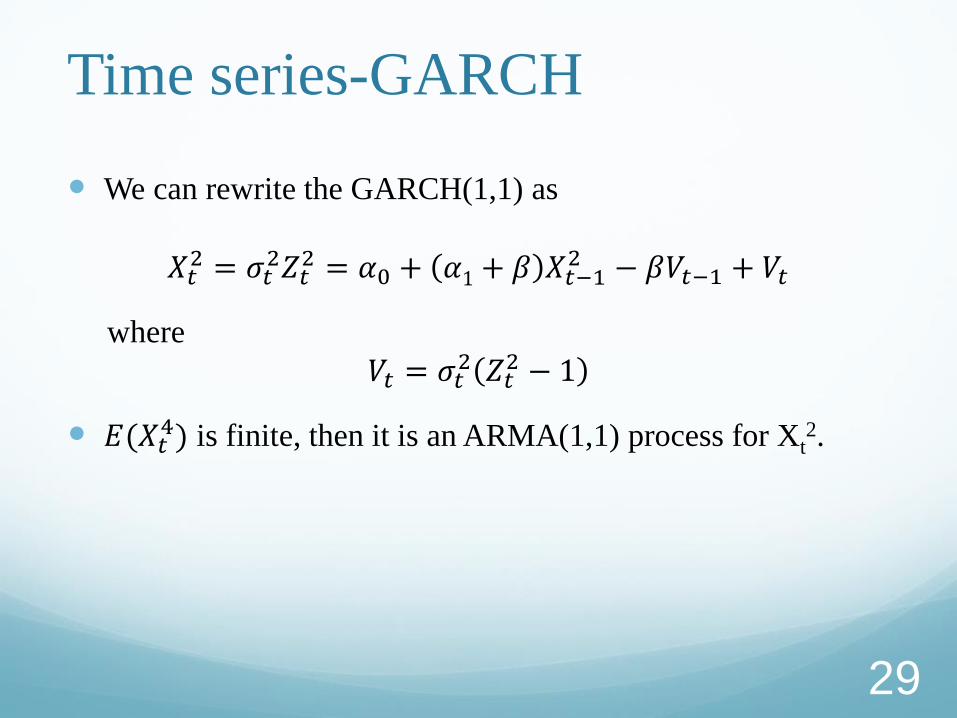
Time series-GARCH

We can rewrite the GARCH(1,1) as

𝑋𝑡2 = 𝜎𝑡

2𝑍𝑡2 = 𝛼0 + 𝛼1 + 𝛽 𝑋𝑡−1

2 − 𝛽𝑉𝑡−1 + 𝑉𝑡

where

𝑉𝑡 = 𝜎𝑡2 𝑍𝑡

2 − 1

𝐸(𝑋𝑡4) is finite, then it is an ARMA(1,1) process for Xt

2.

29

Time series-GARCH

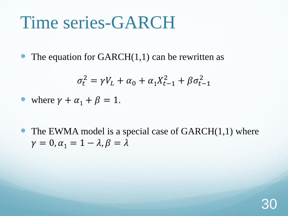
The equation for GARCH(1,1) can be rewritten as

𝜎𝑡2 = 𝛾𝑉𝐿 + 𝛼0 + 𝛼1𝑋𝑡−1

2 + 𝛽𝜎𝑡−12

where 𝛾 + 𝛼1 + 𝛽 = 1.

The EWMA model is a special case of GARCH(1,1) where

𝛾 = 0, 𝛼1 = 1 − 𝜆, 𝛽 = 𝜆

30

Time series-GARCH

The GARCH (1,1) model recognizes that over time the

variance tends to get pulled back to a long-run average level

of 𝑉𝐿 .

Assume we have known 𝜎𝑡2 = 𝑉, if 𝑉 > 𝑉𝐿, then this

expectation is negative

E[s t+1

2 -V | It ] = E[gVL +a1Xt2 + bV -V | It ]

< E[gV +a1Xt2 + bV -V | It ]

= E[-a1V +a1Xt2 | It ]

= -a1V +a1V

= 0

31

Time series-GARCH

If 𝑉 < 𝑉𝐿, then this expectation is positive

This is called mean reversion.

E[s t+1

2 -V | It ] = E[gVL +a1Xt2 + bV -V | It ]

> E[gV +a1Xt2 + bV -V | It ]

= E[-a1V +a1Xt2 | It ]

= -a1V +a1V

= 0

32

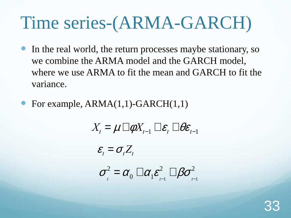
Time series-(ARMA-GARCH)

In the real world, the return processes maybe stationary, so

we combine the ARMA model and the GARCH model,

where we use ARMA to fit the mean and GARCH to fit the

variance.

For example, ARMA(1,1)-GARCH(1,1)

Xt = m +fXt-1 + et +qet-1

et =s tZt

st

2 = a0 +a1e t-1

2 + bst-1

2

33

Time Series in R Data from Starbucks Corporation (SBUX)

34

Program Preparation Packages:

>require(quantmod): specify, build, trade and analyze quantitative financial trading strategies

>require(forecast): methods and tools for displaying and analyzing univariate time series forecasts

>require(urca): unit root and cointegration tests encountered in applied econometric analysis are implemented

>require(tseries): package for time series analysis and computational finance

>require(fGarch): environment for teaching ‘Financial Engineering and Computational Finance’

35

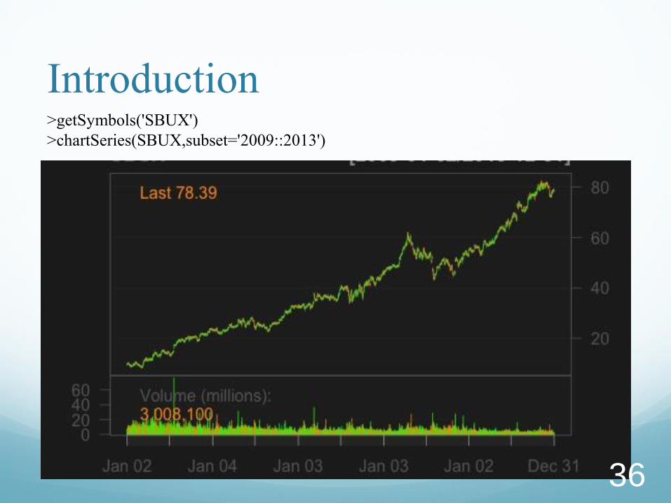
Introduction >getSymbols('SBUX')

>chartSeries(SBUX,subset='2009::2013')

36

Method of Modeling

>ret=na.omit(diff(log(SBUX$SBUX.Close)))

>plot(r, main='Time plot of the daily logged return of SBUX')

37

KPSS test

KPSS tests are used for testing a null hypothesis that an

observable time series is stationary around a deterministic

trend.

The series is expressed as the sum of deterministic trend,

random walk, and stationary error, and the test is the

Lagrange multiplier test of the hypothesis that the random

walk has zero variance.

KPSS tests are intended to complement unit root tests

38

KPSS test

39

𝑥𝑡 = 𝐷𝑡𝛽 + 𝑢𝑡 + ω𝑡

ω𝑡 = ω𝑡−1 + 휀𝑡 휀𝑡~𝑊𝑁(0, 𝜎2)

where 𝐷𝑡: contains deterministic components

𝑢𝑡: stationary time series

ω𝑡: pure random walk with innovation variance

Trend Check

KPSS test: null hypothesis:

>summary(ur.kpss(r,type='mu',lags='short'))

Return is a stationary around a constant, has no linear trend

s2 = 0

40

ADF test

ADF test is a test for a unit root in a time series sample.

ADF test:

∆𝑋𝑡 = 𝛼 + 𝛽𝑡 + 𝛾𝑋𝑡−1 + 𝛿1∆𝑋𝑡−1 + ⋯+ 𝛿𝑝∆𝑋𝑡−𝑝−1 + 휀𝑡

null hypothesis: 𝛾 = 0 ⇒ 𝑋𝑡has unit root

It is an augmented version of the Dickey-Fuller test for a

larger and more complicated set of time series models.

ADF used in the test, is a negative number. The more

negative it is, the stronger the rejection of the hypothesis that

there is a unit root at some level of confidence.

41

Trend Check

ADF Test: null hypothesis: Xt has AR unit root

(nonstationary)

>summary(ur.df(r,type='trend',lags=20,selectlags='BIC'))

Return is a stationary time series with a drift

42

Check Seasonality >par(mfrow=c(3,1))

>acf(r)

>pacf(r)

>spec.pgram(r)

43

Random Component Demean data >r1=r-mean(r)

>acf(r1); pacf(r1);

44

Random Component

>fit=arima(r,order=c(1,0,0))

>tsdiag(fit) AR(1)

45

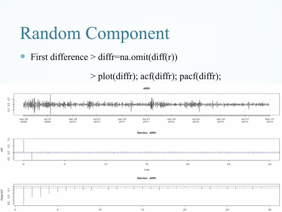
Random Component

First difference > diffr=na.omit(diff(r))

> plot(diffr); acf(diffr); pacf(diffr);

46

Random Component

>fit1=arima(r,order=c(0,1,1)); tsdiag(fit1);

47

Random Component >fit2=arima(r,order=c(1,1,1)); tsdiag(fit2); ARIMA(1,1,1)

48

Model Selection

49

𝐴𝐼𝐶 = 2𝑘 − 2ln (𝐿)

where 𝑘 is the number of parameters, 𝐿 is likelihood

Final model:

𝑋𝑡 = 0.0017 − 0.0724𝑋𝑡−1 + 휀𝑡

Shapiro-Wilk normality test

The Shapiro- Wilk test, proposed in 1965, calculates a W

statistic that tests whether a random sample comes from a

normal distribution.

Small values of W are evidence of departure from normality

and percentage points for the W statistic, obtained via Monte

Carlo simulations.

50

Residual Test

>res=residuals(fit)

>shapiro.test(res) not normally distributed

51

Residual Test

>par(mfrow=c(2,1))

>hist(res); lines(density(res))

>qqnorm(res); qqline(res)

52

ARMA+GARCH

ARMA(1,0)+GARCH(1,1)

>summary(garchFit(~arma(1,0)+garch(1,1),r,trace=F))

ARIMA(1,1,1)+GARCH(1,1)

>summary(garchFit(~arma(1,1)+garch(1,1),data=diffr,trace=F))

53

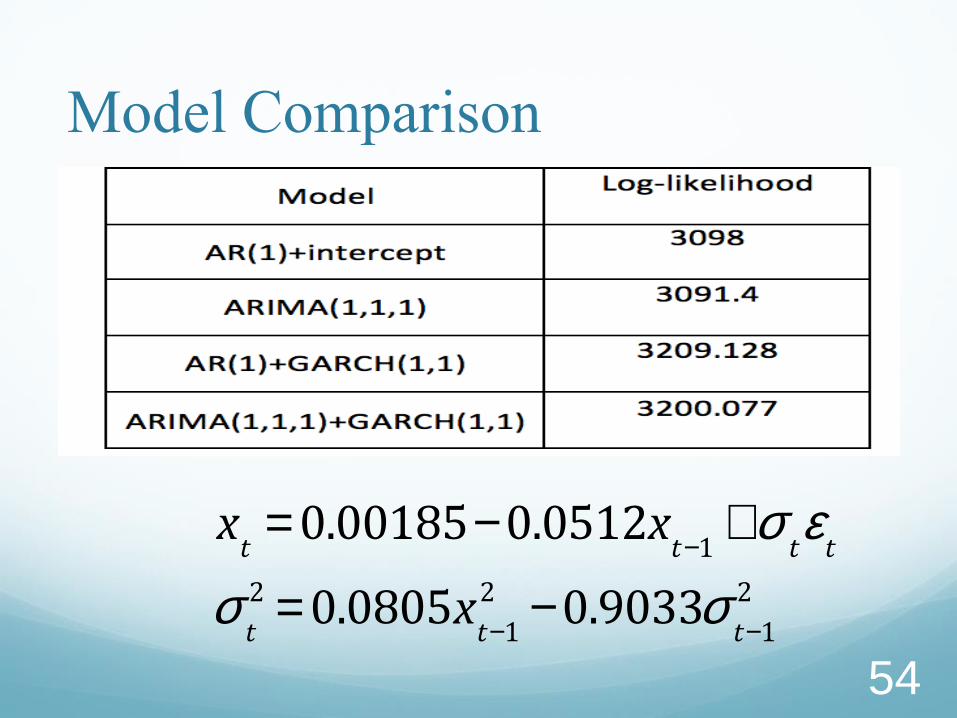
Model Comparison

xt= 0.00185-0.0512x

t-1+s

te

t

st

2 = 0.0805xt-1

2 -0.9033st-1

2

54

Forecasting

55

Time Series in SAS Data from Starbucks Corporation (SBUX)

56

SAS Procedures for Time Series PROC ARIMA

This procedure do model identification, parameter

estimation and forecasting for model ARIMA(p,d,q)

(1 − 𝐵)𝑑𝑋𝑡 = 𝜇 +1 − 𝜃1𝐵 − ⋯− 𝜃𝑞𝐵

𝑞

1 − 𝜙1𝐵 − ⋯− 𝜙𝑝𝐵𝑝𝑍𝑡

where 𝜇 is ground mean of 𝑋𝑡 and

𝜇 1 − 𝜙1𝐵 − ⋯− 𝜙𝑝𝐵𝑝 = 𝜇 1 − 𝜙1 − ⋯− 𝜙𝑝

is the usually intercept (drift).

does NOT do ARCH/GARCH

57

SAS Procedures for Time Series PROC AUTOREG

This procedure estimate and forecast the linear

regression model for time series data with an

autocorrelated error or a heterosedastic error 𝑌𝑡 = 𝑿𝑡𝛽 + 𝜐𝑡

𝜐𝑡 = −𝜙1𝜐𝑡−1 − ⋯− 𝜙𝑝𝜐𝑡−𝑝 + 휀𝑡

휀𝑡 = 𝜎𝑡𝑍𝑡

𝜎𝑡2 = 𝛼0 + 𝛼𝑖휀𝑡−𝑖

2𝑄

𝑖=1+ 𝛾𝑗𝜎𝑡−𝑗

2𝑃

𝑗=1

Independent assumption invalid Autocorrelated error

Homosedasity assumption invalid Heterosedastic error

Linear regression model

Autocorrelated error

Heterosedastic error

58

Import Data

DATA st.return;

INFILE "\SBUXreturn.txt"

firstobs=2;

INPUT Date YYMMDD10. r;

FORMAT Date Date9.;

RUN;

st.return

SBUXreturn.txt

59

PROC SGPLOT DATA=st.return;

SERIES X=Date Y=r;

RUN;

60

Testing for Autocorrelation

The following statements perform the Durbin-Watson test for

autocorrelation in the returns for orders 1 through 3. The

DWPROB option prints the marginal significance levels (p-

values) for the Durbin-Watson statistics.

PROC AUTOREG DATA=st.return;

TITLE2 "AUTOREG AR Test";

MODEL r = / METHOD=ML DW=3 DWPROB;

RUN;

61

Durbin-Watson test If 𝑒𝑡 is the residual associated with the observation at time 𝑡,

then the test statistic is

𝑑 = 𝑒𝑡 − 𝑒𝑡−1

2𝑇𝑡=2

𝑒𝑡2𝑇

𝑡=1

where 𝑇 is the number of observations.

Since

𝑑 = 𝑒𝑡

2𝑇𝑡=1 + 𝑒𝑡−1

2𝑇𝑡=1 − 2 𝑒𝑡𝑒𝑡−1

𝑇𝑡=1

𝑒𝑡2𝑇

𝑡=1

≈ 2 − 2 𝑒𝑡𝑒𝑡−1

𝑇𝑡=1

𝑒𝑡2𝑇

𝑡=1

≈ 2 − 2𝑟 = 2(1 − 𝑟)

where 𝑟 is the sample autocorrelation of the residuals. 62

Durbin-Watson test

Since 𝑑 ≈ 2 1 − 𝑟

Positive serial correlation 0 < 𝑟 < 1 0 < 𝑑 < 2

Negative serial correlation −1 < 𝑟 < 0 2 < 𝑑 < 4

To test for positive autocorrelation at significance α :

If 𝑑 < 𝑑𝐿, 𝛼, the error terms are positively autocorrelated

If 𝑑 > 𝑑𝑈, 𝛼, there is no statistical evidence

• To test for negative autocorrelation at significance α :

If (4 − 𝑑) < 𝑑𝐿, 𝛼, the error terms are negatively autocorrelated

If (4 − d) > 𝑑𝑈, 𝛼, there is no statistical evidence

(𝑑𝐿, 𝛼 and 𝑑𝑈, 𝛼

are lower and upper critical values)

63

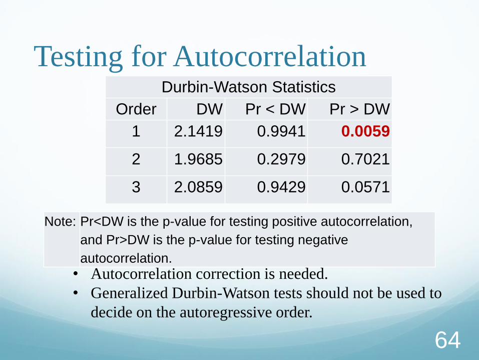
Testing for Autocorrelation Durbin-Watson Statistics

Order DW Pr < DW Pr > DW

1 2.1419 0.9941 0.0059

2 1.9685 0.2979 0.7021

3 2.0859 0.9429 0.0571

Note: Pr<DW is the p-value for testing positive autocorrelation,

and Pr>DW is the p-value for testing negative

autocorrelation.

• Autocorrelation correction is needed.

• Generalized Durbin-Watson tests should not be used to

decide on the autoregressive order.

64

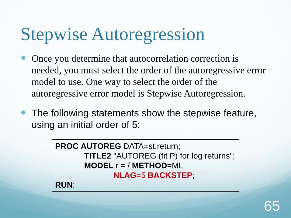
Stepwise Autoregression

Once you determine that autocorrelation correction is

needed, you must select the order of the autoregressive error

model to use. One way to select the order of the

autoregressive error model is Stepwise Autoregression.

The following statements show the stepwise feature,

using an initial order of 5:

PROC AUTOREG DATA=st.return;

TITLE2 "AUTOREG (fit P) for log returns";

MODEL r = / METHOD=ML

NLAG=5 BACKSTEP;

RUN;

65

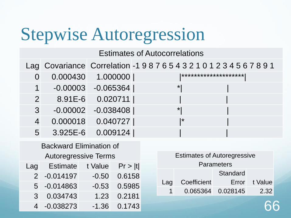
Stepwise Autoregression Estimates of Autocorrelations

Lag Covariance Correlation -1 9 8 7 6 5 4 3 2 1 0 1 2 3 4 5 6 7 8 9 1

0 0.000430 1.000000 | |********************|

1 -0.00003 -0.065364 | *| |

2 8.91E-6 0.020711 | | |

3 -0.00002 -0.038408 | *| |

4 0.000018 0.040727 | |* |

5 3.925E-6 0.009124 | | |

Backward Elimination of

Autoregressive Terms

Lag Estimate t Value Pr > |t|

2 -0.014197 -0.50 0.6158

5 -0.014863 -0.53 0.5985

3 0.034743 1.23 0.2181

4 -0.038273 -1.36 0.1743

Estimates of Autoregressive

Parameters

Lag Coefficient

Standard

Error t Value

1 0.065364 0.028145 2.32

66

Testing for Heteroscedasticity One of the key assumptions of the ordinary regression

model is that the errors have the same variance

throughout the sample. This is also called

the homoscedasticity model. If the error variance is

not constant, the data are said to be Heteroscedastic

The following statements use the ARCHTEST= option

to test for heteroscedasticity

PROC AUTOREG DATA=st.return;

TITLE2 "AUTOREG arch Test";

MODEL r = / METHOD=ML ARCHTEST;

RUN;

67

Testing for Heteroscedasticity Portmanteau Q Test

For nonlinear time series models, the portmanteau test statistic based

on squared residuals is used to test for independence of the series

𝑄 𝑞 = 𝑇 𝑇 + 2 𝑟 𝑖; 𝑒 𝑡

2

𝑁 − 𝑖

𝑞

𝑖=1

where

𝑟 𝑖; 𝑒 𝑡2 =

𝑒 𝑡2 − 𝜎 2 𝑒 𝑡−𝑖

2 − 𝜎 2𝑇𝑡=𝑖+1

𝑒 𝑡2 − 𝜎 2 2𝑇

𝑡=1

𝜎 2 =1

𝑇 𝑒 𝑡

2

𝑇

𝑡=1

68

Testing for Heteroscedasticity Lagrange Multiplier Test for ARCH Disturbances

Engle (1982) proposed a Lagrange multiplier test for ARCH disturbances. Engle’s Lagrange multiplier test for the qth order ARCH process is written

𝐿𝑀 𝑞 =𝑇𝑊′𝑍 𝑍′𝑍 −1𝑍′𝑊

𝑊′𝑊

where

𝑊 =𝑒 12

𝜎 2, … ,

𝑒 𝑇2

𝜎 2

′

, 𝑍 =

1 𝑒 02 … 𝑒 −𝑞+1

2

⋮ ⋮ ⋮ ⋮⋮ ⋮ ⋮ ⋮1 𝑒 𝑁−1

2 … 𝑒 𝑁−𝑞2

The presample values 𝑒 02, … , 𝑒 −𝑞+1

2 have been set to 0 69

Tests for ARCH Disturbances Based on OLS

Residuals

Order Q Pr > Q LM Pr > LM

1 3.3583 0.0669 3.3218 0.0684

2 20.6045 <.0001 19.7499 <.0001

3 30.4729 <.0001 27.3240 <.0001

4 32.0168 <.0001 27.5946 <.0001

5 40.3500 <.0001 32.2671 <.0001

6 45.0011 <.0001 34.6383 <.0001

7 53.2330 <.0001 38.9149 <.0001

8 74.7145 <.0001 52.6820 <.0001

Testing for Heteroscedasticity

The p-values for the test statistics strongly indicate

heteroscedasticity 70

Fitting AR(p)-GARCH(P,Q) The following statements fit an AR(1)-GARCH model

for the return r. The GARCH=(P=1,Q=1) option

specifies the GARCH conditional variance model. The

NLAG=1 option specifies the AR(1) error process.

PROC AUTOREG DATA=st.return;

TITLE2 "AR=1 GARCH(1,1)";

MODEL r = / METHOD=ML NLAG=1

GARCH=(p=1,q=1);

OUTPUT OUT=st.rout HT=variance P=yhat

LCL=low95 UCL=high95;

RUN;

71

Fitting AR(1)-GARCH(1,1)

Parameter Estimates

Variable DF Estimate

Standard

Error t Value

Approx

Pr > |t|

Intercept 1 0.001778 0.000476 3.74 0.0002

AR1 1 0.0512 0.0330 1.55 0.1203

ARCH0 1 7.8944E-6 1.6468E-6 4.79 <.0001

ARCH1 1 0.0804 0.009955 8.08 <.0001

GARCH1 1 0.9041 0.0110 81.91 <.0001

𝑟𝑡 = 0.001778 + 𝜐𝑡 𝜐𝑡 = −0.0512𝜐𝑡−1 + 휀𝑡 ,

휀𝑡 = 𝜎𝑡𝑍𝑡 , 𝜎𝑡

2 = 7.89 × 106 + 0.0804휀𝑡−12 + 0.9041𝜎𝑡−1

2

72

Fitting GARCH(1,1)

𝑟𝑡 = 0.001789 + 휀𝑡 , 휀𝑡 = 𝜎𝑡𝑍𝑡 ,

𝜎𝑡2 = 8.23 × 106 + 0.0824휀𝑡−1

2 + 0.9014𝜎𝑡−12

Parameter Estimates

Variable DF Estimate

Standard

Error t Value

Approx

Pr > |t|

Intercept 1 0.001789 0.000500 3.58 0.0003

ARCH0 1 8.2257E-

6

1.7139E-

6

4.80 <.0001

ARCH1 1 0.0824 0.0103 8.04 <.0001

GARCH1 1 0.9014 0.0114 78.91 <.0001

73

Model Comparison AR(1)-GARCH(1,1) GARCH(1,1)

GARCH Estimates

SSE 0.5350539

1

Observations 1258

MSE 0.0004253 Uncond Var 0.0005082

9

Log

Likelihood

3208.0508

4

Total R-

Square

0.0048

SBC -

6380.4153

AIC -

6406.1017

MAE 0.0143874

4

AICC -

6406.0538

MAPE 115.69169

2

HQC -

6396.4484

Normality Test 1079.9508

Pr > ChiSq <.0001

GARCH Estimates

SSE 0.5376265

2

Observations 1258

MSE 0.0004274 Uncond Var 0.0005083

7

Log

Likelihood

3206.7125

6

Total R-

Square

.

SBC -6384.876 AIC -

6405.4251

MAE 0.0144074

5

AICC -

6405.3932

MAPE 113.75148

9

HQC -

6397.7025

Normality

Test

1054.2731

Pr > ChiSq <.0001

74

Prediction

75

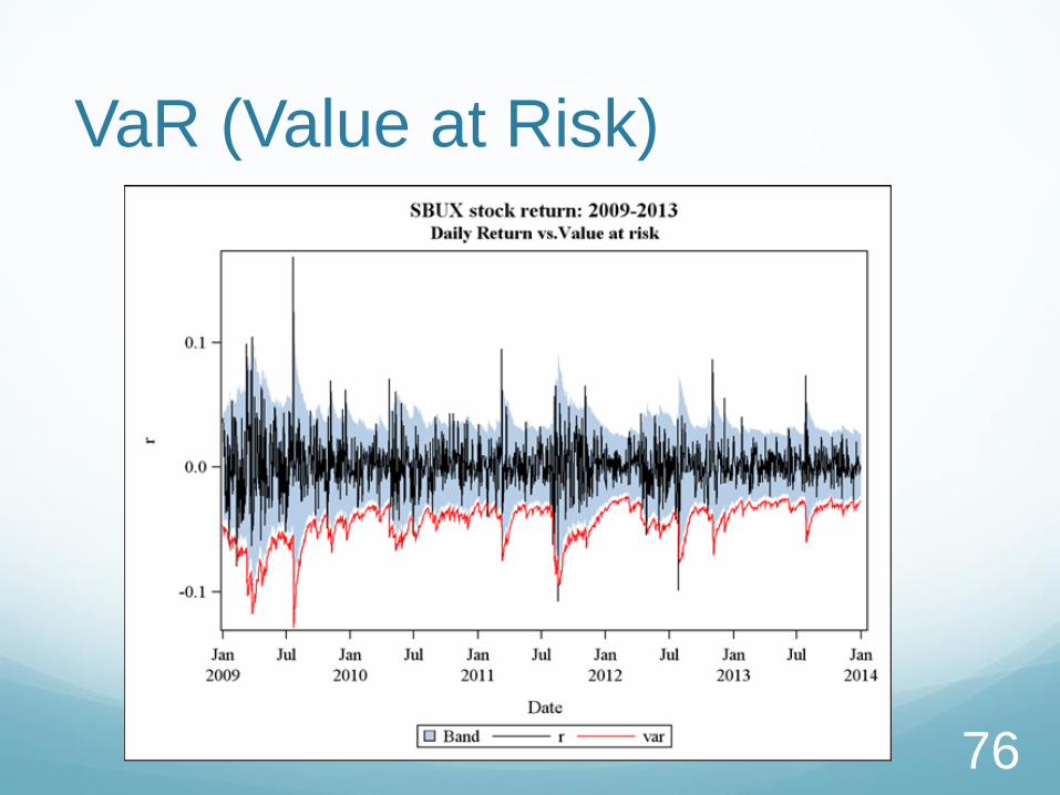
VaR (Value at Risk)

76

Summary Models for conditional variance (risk)

ARCH

EWMA

GARCH

Numerical experiment

ARIMA+GARCH in R

AR+GARCH in SAS

VaR in SAS

77

78

This presentation was

revised from my

students’ presentation.

青出于蓝，而胜于蓝