Bargaining, Search and Outside Options

Anita Gantner�

Department of Economics

University of California, Santa Barbara

Preliminary Version

January 18, 2002

Abstract

This paper studies a bargaining model between a buyer and a

seller, where both agents have incomplete information about the op-

ponent's valuation for the good to be traded, and where the buyer's

outside option is to buy via search. The model extends the Chatterjee

and Samuelson (1987) model by introducing an outside option which

is modelled and as a standard sequential search process, where the

buyer can choose to search and return to bargaining at any time. We

distinguish two regimes for the search process: In Regime I, the ex-pected return from search is used as an outside option. Here we �nd

that the option to return to the bargaining table is redundant and only

the search parameters are relevant for the buyer's decision to quit the

bargaining partner and start search. In Regime II, the buyer has to

use actual o�ers as a valid outside option. Here the results show how

the conditions to start search and to continue search di�er.

Keywords: Bargaining, Incomplete Information, Outside Option, Search

JEL Classi�cation: C78, D83, C61

�Department of Economics, University of California, Santa Barbara, CA 93106, Email:gantner@econ.ucsb.edu. I would like to thank Ted Bergstrom, Ken Binmore, John McCall,Chris Proulx, Cheng-Zhong Qin and Larry Samuelson for helpful comments. Specialthanks to Morten Bech for discussions and encouragement.

1

1 Introduction

One of the most basic situations in economic analysis is when a buyer and aseller trade one unit of an indivisible good, both agents seeking to maximizetheir individual surplus. A simple setting like this can answer importantquestions like: When will the agents trade? What will the price be? Who willget the highest surplus? Of course, it depends on the exact circumstances, orthe \rules of the game", how these questions will be answered. For example,if a seller and a buyer meet and bargain, the analysis will be di�erent fromthe situation where a buyer can choose to accept one of many non-negotiableprice o�ers from di�erent sellers, which he receives at di�erent times.

In a bargaining situation, it also depends on the rules of bargaining andthe available information about agents and their strategies how the equi-librium price is determined and how the surplus is allocated. Rubinstein's(1982) model (or some modi�ed version thereof) is commonly used to describethe bargaining procedure where two agents alternate in proposing prices andthe good is traded as soon as one party accepts a proposal. This modelhas been extended in order to analyze equilibrium strategies when thereis incomplete information (see for example Fudenberg/Tirole (1983) for atwo-period model with one-sided and two-sided incomplete information, Ru-binstein (1985) for one-sided incomplete information with an in�nite timehorizon, Chatterjee and Samuelson (1987) for two-sided incomplete informa-tion in an in�nite time horizon model).

On the other hand, when prices are posted and non-negotiable, and buyerscan look around for the best o�er, a search theoretic approach using Bellman'sprinciple of dynamic optimality is useful to answer the fundamental questionof price, surplus and timing of trade. Elementary search models and theirapplications, as presented in Lippman and McCall (1976) and (1981), showhow to �nd the optimal reservation price and how to derive the optimalstopping rule when an agent, who seeks to maximize his surplus, faces a givendistribution of price o�ers and search is costly. In a more recent paper, Arnoldand Lippman (1998) analyze a seller's choice between posting a price andbargaining in a model with incomplete information about buyers' valuationsand their bargaining abilities.

How can bargaining and search models be connected? There are twoobvious ways to do this:

2

(i) The game starts in a search process where an agent is looking for anotheragent to trade with, that is, a particular match is not yet formed. Oncetwo agents are matched, they start to bargain over the price. Mortensen(1982) is one of the early models that incorporate bargaining in a searchand matching model, following the game theoretic approaches of papers byDiamond and Maskin (1979) and Mortensen (1978). These models, however,put less emphasis on the bargaining process. They assume that agreementsare instantaneous where the available surplus is divided in a predeterminedway. A natural candidate is, of course, Nash's axiomatic bargaining so-lution, according to which the surplus is divided equally. Rubinstein andWolinsky (1985) treat the bargaining problem with the strategic approach,which, as they remark, \constitutes an attempt to look into the bargainingblack-box", hence complementing the above mentioned literature. However,their matching technology is not modelled explicitly, and searching simplymeans considering a �xed probability of meeting an agent of the oppositetype.

(ii) The game starts with the bargaining process of a particular pair ofmatched agents.1 Here, at least one agent has an outside option, which is toleave the current bargaining partner in order to look for a higher surplus. Thiscan be modelled as a search process. Applying the outside option principle(see Binmore (1985), Shaked and Sutton (1984)), the paper by Bester (1985)looks at a model where a buyer chooses a bargaining partner from a setof heterogeneous producers at random. The buyers can choose to quit theircurrent partner and search for another seller. Since switching is costly and allconsumers are identical, each buyer meets exactly one seller in equilibriumand the \right" price is proposed immediately. A model with an explicitsearch theoretic approach is Baucells and Lippman (1999), where a sellerknows a speci�c buyer with whom he can bargain over a good. The seller'soutside option is to sell the good via search, that is, by accepting one of theincoming non-negotiable o�ers described by a given probability distribution.The Nash bargaining solution is applied to solve the bargaining problem,which results in an equal split of the surplus. Their focus is not on thebargaining process but the impact of the buyer's availability on the payo�sto both agents.

Looking at the cited literature, it seems that the models that use an ex-

1Equivalently, agents of opposite type meet with certainty in a market model.

3

plicit search theoretic approach do not give much attention to the bargainingprocess, while in the models with an outside option that take a closer lookin the \bargaining black-box", negotiation takes place immediately and theoutside option only a�ects the division of the surplus, but not the timing.

The \no-search solution" of bargaining problems is not completely satis-fying, given that in real-life bargaining situations immediate trade is rarelyobserved or even expected. Bargainers often hesitate to take the �rst o�er;they search, hoping to get a better outcome than if they just accepted the�rst o�er. The bargaining models described above seem to lack some impor-tant features that make search more likely. Intuitively, the result of no searchin equilibrium may change once we allow for heterogeneity in buyers' valu-ation and sellers' cost. For example, if a buyer is matched with a high-costseller, it might be worth for him to search a little longer to �nd a low-costseller who can o�er him a better price even though search is costly.

This paper analyzes a situation where a buyer and a seller are matchedand they start bargaining. The bargaining process is described by a versionof Rubinstein's alternating o�ers game. Neither agents knows the opponent'sexact valuation for the good to be traded. The buyer has an outside optionwhich is to buy the good via search by accepting one of the non-negotiableo�ers that are assumed to arrive in accordance with a given distribution.Thus, the model interlaces a search process and a bargaining process.

The paper is organized as follows: Section 2 outlines the complete bar-gaining - search model. In section 3, we will look at the bargaining problemtaking the outside option as given, hence solving a two-sided incomplete in-formation bargaining problem with an outside option. Having solved thebargaining problem with a given outside option, the solution will be incorpo-rated in the search theoretic analysis in section 4. The goal of this paper is tosolve a search problem by explicitly considering the bargaining problem in-volved, which captures important elements of a bargaining process, includingincomplete information about agents' valuation and an outside option.

4

2 Motivation of the Model: An Example

Suppose buyer B seeks to buy a house and he happens to know a speci�cseller S who is willing to sell his house. This house has exactly the featuresB is looking for and B doesn't know of any other suitable house for sale atthis time. Both B and S are imperfectly informed about the other agent'svaluation for the house. S is not sure whether the particular features of thishouse are very important for B, in which case B would be willing to pay ahigh price vh, or if they are of minor importance, in which case B is onlywilling to pay a low price vl, where vl < vh. B, on the other hand, is not surewhether S considers his house to be of high value ch or low value cl, whichdetermines the lowest price S would be willing to accept.

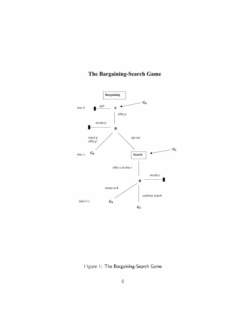
The bargaining between B and S is modelled according to Rubinstein'salternating-o�ers procedure with the following modi�cation: In each round,S can either quit or o�er a price p. In the same round, B responds withone of three choices: accepting p, rejecting p and making a countero�er p0,or opting out. The outside option is to buy via search. Search is modelledin the standard way: non-negotiable o�ers y arrive according to a Poissonprocess with arrival rate � > 0 and E[y] < 1. The time interval betweensuccessive arrivals of o�ers is distributed exponentially.

The game form of the bargaining-search game is illustrated in Figure 1.Let G denote a subgame starting in the bargaining phase and N denote asubgame starting in the search phase. In the bargaining phase, B immediatelyresponds to S's o�er p. If he accepts p, the game is over. If he rejects p andmakes a countero�er, the bargaining proceeds to the next round, which takes� time units and another (identical) subgame G starts. If B opts out, thesubgame N starts immediately, where B searches until he locates an outsideo�er. During this time, there are no decisions to be made by either player.When B locates an outside o�er y at time t, he has to choose between oneof three options: he can accept y and the game is over, or he can continuesearch and another (identical) subgame N starts, or he can return to bargainwith S, which will take him � time units and bring him back to the subgameG.

The payo�s to the players are now described. Let r be the common rate oftime preference for both players. For notational convenience of the discountfactor, let e�r� be denoted by �. If the game is terminated by an agreement

5

B

S

offer p

accept p

reject p

offer p’

opt out

Search

time 0

offer y at time t

time �

B

accept y

GB

GS

GB

GS

time t+�

GB

Bargaining

return to S

continue search

The Bargaining-Search Game

quit

Figure 1: The Bargaining-Search Game

6

between B and S over a price p at time t + �, B receives (v � p)�e�rt forv = vh; vl depending on whether he has a high valuation or a low valuationfor the house. S receives (p� c)�e�rt for c = ch; cl depending on his cost. Ifthe game is terminated by B accepting an outside o�er y at time t, B receivesa payo� of (v� y)e�rt for v = vh; vl depending on the buyer's valuation, andS receives zero. In case B and S perpetually disagree or if B searches forever,the payo�s are zero for each player.

Muthoo (1995) looks at a similar game that interlaces a bargaining gamewith a search process, however, in his model agents have complete informa-tion. He shows that the option of returning to the old bargaining partnerafter having searched for some �nite time does not a�ect the unique subgameperfect equilibrium. In other words, the outcome does not depend on whetheror not a bargainer is allowed to choose to return to the negotiating table.He concludes that this result depends crucially on the complete informationassumption and the stationarity of the move-structure of the game.

In this paper, the solution of the bargaining-search game with incompleteinformation about agents' valuations shall be approached by looking at thetwo processes separately at �rst and connecting them later. In the nextsection we will analyze how a given outside option changes the equilibriumstrategies in the bargaining model with two-sided incomplete information.

3 The Bargaining Problem

The bargaining-search problem described in section 2 includes an explicitbargaining process, which will be modelled according to the following char-acteristics:

� each agent is uncertain about the valuation of the opponent

� there are no exogenous restrictions on the duration of the game

� each agent can quit the negotiations at the end of each period

� the buyer can purchase the good via search (outside option)

� the gains from bargaining depend on the characteristics of the agentsand their outside options.

7

A model with these characteristics can be described as a non-cooperativebargaining problem with two-sided incomplete information and outside op-tion. The following analysis is based on the Chatterjee and Samuelson (1987)model of bargaining with two-sided incomplete information, but additionally,it has a �xed outside option for the buyer. To point it out again, the ideaof this paper is to solve the \bigger" problem where the bargaining solu-tion is incorporated in the search problem. However, �rst we shall see howthe outside option changes the equilibrium strategies in the Chaterjee andSamuelson model.

With complete information, the introduction of an outside option hasbeen studied in the literature, e.g. the \outside option principle" in Binmore(1985) when the Nash bargaining solution is applied, Rubinstein and Wolin-sky (1985), which incorporates an outside option in an alternating-o�ersbargaining process, or Chatterjee and Lee (1993), where there is incompleteinformation about the outside option.

When modelled explicitly, the outside option can be described by anarrival of o�ers according to a Poisson process with some given arrival rateand cumulative distribution function (see e.g. Baucells and Lippmann (1999),Muthoo (1995)). In the following subsection, we will treat it as a given value,�MN , and solve the bargaining problem as such. Afterwards, the value of �MN

will be modelled as the value of buying the good via search, including theoption to return to bargaining. Thus, �MN will be determined endogenouslyfrom the optimal search policy.

3.1 The Bargaining Model

Consider a bargaining game between two types of agents, a seller S and abuyer B. S is endowed with one indivisible unit of a good. He can be oneof two possible types: a high-cost seller with a valuation of ch for the goodor a low-cost seller with a valuation of cl. Similarly, B has either a highvaluation of vh or a low valuation of vl for the good. We will assume thatcl � vl < ch � vh. Since both the low-cost seller and the high-valuationbuyer can trade with bargaining partners of any type and hence have some exibility in the price they can o�er, they shall be called exible agents. Thehigh-cost seller and the low-cost buyer shall be called in exible agents. Thefollowing table summarizes the agents' type and valuation:

8

Seller Buyerin exible ch vl

exible cl vh with cl � vl < ch � vh

At time 0, the buyer's prior probability that the seller is exible is �S ,and 1 � �S is his probability that the seller is in exible. For the seller, hisprior probability that the buyer is exible is �B and the probability thatthe buyer is in exible is 1 � �B. The priors �S and �B are assumed to begiven exogenously and are common knowledge. Agents update their beliefsaccording to Bayes' rule.

The bargaining procedure is as follows: In round 1, the seller �rst o�ers aprice p, at which he is willing to exchange the good. Then the buyer makesa countero�er. If the two o�ers are compatible, that is, mutually acceptabletrade is possible, the game ends with trade. The seller's payo� is p � ch

if he is a high-cost seller and p � cl if he is a low-cost seller. The buyer'spayo� from the purchase is vh � p if he is a high-valuation buyer and vl � p

if he is a low-valuation buyer. If the two o�ers are not compatible, the buyercan choose between two possible moves: He may quit the seller and take hisoutside option, yielding a payo� of �MN for the buyer, with 0 � �MN <1, andzero for the seller. Or, he may choose to continue bargaining with the sellerand o�er p0. In this case, bargaining proceeds to the next round, which takes� units of time and hence, payo�s are discounted by a common discountfactor � and the sequence of o�ers begins again.2

Chatterjee and Samuelson (1987) examine a similar game of two-sidedincomplete information without an outside option. They restrict the o�ersto come from the set fvl; chg, that is, there are only two possible strate-gies for each agent: vl is the low price o�er and ch is the high price o�er.They justify the restriction to the set [vl; ch] by the idea that if there areknown in exible agents who are willing to trade at their valuation, acceptingany o�er outside this interval is dominated by trading with these in exibleagents. The further restriction to the two-element set fvl; chg implies thatgains from trade will go entirely to either the buyer or the seller and seems

2This process di�ers slightly from Rubinstein's alternating o�ers game, where playersalternate in o�er periods. However, as Chatterjee and Samuelson (1987) remark, thischanges only the calculation of ��S and ��B later on, but leaves the rest of the analysisuna�ected.

9

quite strong in its implications. As they show, this game has a unique Nashequilibrium. In the potentially in�nite horizon game, bargaining proceedsonly for a �nite but endogenously determined number of periods, since thenonzero probability that the opponent is in exible �xes some limit beyondwhich a exible bargainer will never continue.

In Chatterjee and Samuelson (1988), the model without restriction on theo�ers is examined. Unlike the restricted model, there are multiple equilibria,including the one which shares the features of the restricted-o�ers case. Theauthors favor the latter as selection of a unique equilibrium by arguments ofplausibility. They emphasize that the multitude of equilibria does not alterthe model's qualitative results and implications for bargaining. In view ofthese �ndings, the restricted-o�ers case shall be considered in this paper, inorder to simplify the analysis while retaining the important aspects of themodel. In the following, since there are only these two strategies availablefor each agent, we shall call ch the high price o�er and vl the low price o�er.

The immediate implications of the setup are that if S o�ers the high priceand B the low price, no trade will occur; only if both agents o�er the highprice or both o�er the low price, trade may occur. The case where S o�ersthe low price and B o�ers the high price does not have to be considered, sinceif S o�ers the low price, B will certainly have no incentive to respond witha high price o�er and vice versa. If both agents are in exible, o�ering theirtrue valuation is dominant, hence an in exible S always o�ers the high priceand an in exible B always o�ers the low price. Since an in exible buyer willnever trade with an in exible seller, he will surely take his outside option,once he concludes that his opponent is an in exible agent as well.

3.2 Equilibrium Analysis

The analysis will closely follow the Chatterjee and Samuelson (1987) model,however, in the present model the buyer's outside option has to be consideredwhen looking at equilibrium strategies. We expect this to in uence the equi-librium strategies, since we know that exible agents will try to masqueradeas in exible ones, and the outside option may help the buyer to reveal theseller's identity.

In our model, since for in exible agents o�ering their true valuation isdominant (otherwise they would have a negative payo�), we only have to

10

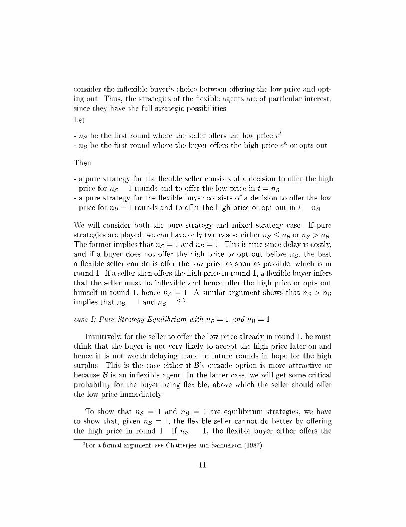
consider the in exible buyer's choice between o�ering the low price and opt-ing out. Thus, the strategies of the exible agents are of particular interest,since they have the full strategic possibilities.

Let

- nS be the �rst round where the seller o�ers the low price vl

- nB be the �rst round where the buyer o�ers the high price ch or opts out

Then

- a pure strategy for the exible seller consists of a decision to o�er the highprice for nS � 1 rounds and to o�er the low price in t = nS .

- a pure strategy for the exible buyer consists of a decision to o�er the lowprice for nB � 1 rounds and to o�er the high price or opt out in t = nB.

We will consider both the pure strategy and mixed strategy case. If purestrategies are played, we can have only two cases: either nS � nB or nS > nB.The former implies that nS = 1 and nB = 1. This is true since delay is costly,and if a buyer does not o�er the high price or opt out before nS , the besta exible seller can do is o�er the low price as soon as possible, which is inround 1. If a seller then o�ers the high price in round 1, a exible buyer infersthat the seller must be in exible and hence o�er the high price or opts outhimself in round 1, hence nB = 1. A similar argument shows that nS > nBimplies that nB = 1 and nS = 2.3

case I: Pure Strategy Equilibrium with nS = 1 and nB = 1

Intuitively, for the seller to o�er the low price already in round 1, he mustthink that the buyer is not very likely to accept the high price later on andhence it is not worth delaying trade to future rounds in hope for the highsurplus. This is the case either if B's outside option is more attractive orbecause B is an in exible agent. In the latter case, we will get some criticalprobability for the buyer being exible, above which the seller should o�erthe low price immediately.

To show that nS = 1 and nB = 1 are equilibrium strategies, we haveto show that, given nB = 1, the exible seller cannot do better by o�eringthe high price in round 1. If nB = 1, the exible buyer either o�ers the

3For a formal argument, see Chatterjee and Samuelson (1987).

11

high price or opts out in round 1. In order for him to opt out, it has to bethat �MN > vh � ch, that is, the value of the outside option is greater thanthe surplus he would get if he reveals his type and accepts the seller's highprice. This shall be called a \good" outside option.4 Given that the exiblebuyer has a good outside option, the exible seller can do no better in purestrategies than reveal his type in round 1 by o�ering the low price vl, sincethe high price ch would give him a payo� of zero if the buyer he faces is exible and opts out. In case the seller faces an in exible buyer, he certainlycannot trade by o�ering ch, hence o�ering vl would be optimal independentof the hard buyer's outside option value.5

Given that the outside option is \bad", that is, �MN < vh � ch, nB = 1means that the exible buyer will o�er the high price to the seller in round1. Then the exible seller's best response will be to o�er the low price andreveal his type in round 1 only if o�ering vl and receiving vl � cl in round 1is better than o�ering the high price ch, when the buyer will accept this inround 1 with probability �B and with probability 1� �B the game continuesto the next round:

�B(ch � cl) + �(1� �B)(v

l � cl) � vl � cl (1)

which gives a boundary for �B

�B �(vl � cl)(1� �)

ch � cl � �(vl � cl)� ��B (2)

The expression on the LHS of (1) follows from the fact that round 2 isreached only if the buyer is in exible, which causes the seller to reveal histype in round 2, and hence yielding the expected payo� of �(1� �B)(v

l � cl)for the seller. The boundary ��B identi�es when a prior �B is su�ciently lowfor a exible seller to reveal his type in the �rst round of bargaining. Hence,

4In the bargaining analysis, we will not explicitly consider the case where �MN > vh�vl,since in this case it is clear that the buyer will opt out irrespective of what the seller o�ers.

5Even though the two types of buyers can have di�erent values for their outside options,it is not very interesting to consider the in exible buyer's outside option, since the onlycase where it might a�ect strategies is when the exible buyer's outside option is bad andthe in exible buyer's is good. This should give the seller and incentive to make a weako�er to ensure that he trades with the buyer. However, since the in exible buyer's surplusis at most zero from trading with the seller, we assume that he will choose to opt out ifhis �MN is good, since it o�ers him more than zero.

12

nS = 1 and nB = 1 are equilibrium strategies if the outside option is goodor if �B < ��B. In the equilibrium with trade, the exible seller o�ers thelow price (nS = 1) and his payo� will be vl � cl. The exible buyer receivesvh � vl and the in exible buyer receives 0. Notice that neither of the twotypes of buyers can be made better o� from trading with S than in this casewhere the seller o�ers vl. Since the priors and the outside option are commonknowledge, if �B < ��B an observed high price o�er from a seller in round 1will lead a buyer to the conclusion that the seller must be in exible.

As long as there is a bad outside option and the seller o�ered ch in round 1,a exible buyer cannot improve upon making a revealing o�er. An in exiblebuyer cannot trade with an in exible seller, thus he will certainly opt outin round 1.6 The game in case I ends after the �rst round, however, notnecessarily with trade. Search is possible if at least one of the agents isin exible.

case II: Pure Strategy Equilibrium with nS = 2 and nB = 1

Intuitively, an equilibrium where the seller does not immediately revealhis type will exist if the buyer's outside option is bad and if S thinks thatB is likely to be exible. On the other hand, in order for the exible buyerto o�er the high price in round 1, his prior that S is in exible should besu�ciently high. Thus, the equilibrium will be determined by both a criticallevel of ��B and ��S .

From case I we know that if B's outside option is bad and �B > ��B, the exible seller will not reveal his type in round 1. The optimal strategy forthe exible seller depends on what the exible buyer does, thus the latterhas to be considered �rst.

The following condition for a exible buyer to o�er the high price inround 1 re ects the fact that if the game proceeds to round 2, we know thatnS > nB ) nS = 2 and therefore the exible seller will o�er vl in round 2:

��S(vh � vl) + �(1� �S)(v

h � ch) � vh � ch (3)

The boundary for �S is then given by

6If his outside option is bad, he will search forever.

13

�S �(vh � ch)(1� �)

�(ch � vl)� ��S (4)

Hence, if �B > ��B and �S � ��S , the exible buyer is better o� o�ering thehigh price in round 1, given that he has a bad outside option, and nS = 2and nB = 1 are equilibrium strategies.

If the outside option is good, the exible buyer would opt out rather thano�ering the high price in round 1. Since a seller will be left with a payo�of zero if the buyer opts out, the exible seller will choose to reveal his typeand o�er the low price in round 1, even though he thinks it is likely that thebuyer he faces is exible. As described in case I, a good outside option helpsthe buyer to unravel the seller's type and get the higher surplus in case theseller is exible. The in exible buyer remains in the game as long as he hassome positive probability that the seller is exible. In equilibrium, he willknow this by round 2: for the exible buyer, the game is over after round 1(nB = 1) and hence, a exible seller's optimal strategy must be nS = 2. Ifa seller has not o�ered the low price by round 2, an in exible buyer shouldopt out in round 2.

In the pure strategy equilibrium considered so far, the outside option isonly taken if at least one of the bargaining parties is in exible. The ine�cientcase where the outside option is chosen even though both players are exiblebut hide behind the incomplete information does not occur since the outsideoption is common knowledge and therefore helps the buyer to reveal theseller's type. Also, the outside option only in uences decisions in round 1: itcan make the exible seller change his optimal strategy from o�ering the highto o�ering the low price. Since the equilibrium in pure strategies requires the exible buyer to end the game in round 1, the outside option a�ects the pureequilibrium strategies only in round 1.7 Things can be di�erent in a mixedstrategy equilibrium. As we know from the game without outside options,bargaining will continue for an endogenously determined number of roundswhen agents randomize. The role of the outside option is not necessarilytrivial then.

case III: Mixed Strategy Equilibrium

7This is true for the �xed outside option. Later on, we will consider the option toreturn to bargaining after searching for some time.

14

Before we look at the mixed strategies, some logical conclusions for theNash Equilibrium from the Chatterjee and Samuelson model should be statedhere.

� A exible agent will never continue the game inde�nitely, i.e. thereexists some round T beyond which a exible agent will not proceed.8

To see the idea behind this, take the case of a exible seller who willwait to o�er the low price in round t only if the buyer will o�er the highprice in t with su�ciently high probability, so that it doesn't pay for Sto o�er the low price already in t�1. Since the probability of B o�eringthe high price cannot be bounded away from zero in every period, itmust eventually become arbitrarily small. Then there must be some Tsuch that the exible seller will o�er the low price and the game ends.A similar argument holds for B where there is some T beyond whichhe will not continue the game.

� A exible agent will immediately make the o�er that gives him the lowsurplus if he infers that the opponent is in exible. Following the abovelogic, if round T is reached, by which a exible agent would have endedthe game, his opponent infers that the agent is in exible and makesthe for him disadvantageous o�er himself. A direct implication is thenthat the game must have a �nite horizon if at least one of the players is exible. In other words, the potentially in�nite horizon game will havea �nite horizon.

If both agents have low priors that the opponent is exible, that is, if�B > ��B and �S > ��S , there is no equilibrium in pure strategies in the gamewithout outside options. The reason is that since in exible agents want toidentify themselves as in exible and exible agents want to pretend theyare in exible, both agents would give the same signal. Thus, there is nonew information to update the priors, and from the �rst round the priorprobability that the opponent is in exible is not su�ciently high, since both�S > ��S and �B > ��B. Hence, pretending to be an in exible agent might notlead to a success and is therefore not an equilibrium strategy. On the otherhand, it is also not an equilibrium strategy for a exible agent to o�er the forhim disadvantageous price with certainty, since this would lead to a perfect

8For a formal proof, see Chatterjee and Samuelson (1987).

15

distinction of the two types and thus make a deviation therefrom pro�table.How should exible agents randomize?

In the Chatterjee and Samuelson model, the mixed strategy equilibriumis constructed in the following way: Each randomization is determined suchthat the previous agent is indi�erent between the revealing and concealingo�er. This supports the previous agent's randomization. Thus, we get asequence of probabilities until the �rst round T where the probabilities exceedone. This identi�es the round T by which a exible agent has stopped inequilibrium, where T is determined endogenously.

The question in the present model is how the outside option changes thisreasoning. Does the seller have to make the buyer indi�erent between stayingin the game and taking the outside option in every round? Or does he haveto randomize such that the buyer is indi�erent between revealing his typeand the maximum of the following two: outside option and expected payo�of randomizing as in the game without outside options? To analyze this, thefollowing notation will be useful: In the game without outside options, letqiSbe a seller's probability that he plays a pure strategy with nS = i and qi

B

be a buyer's probability that he plays a pure strategy with nB = i, whereP1

i=1 qiS= 1 and

P1

i=1 qiB= 1. Then fqi

Sg shall denote a exible seller's mixed

strategy and fqiBg shall denote a exible buyer's mixed strategy.

Let EiS= expected payo� to a exible seller from playing a pure strategy

with nS = i

EiB= expected payo� to a exible buyer from playing a pure strategy

with nB = i

Hence

EtS=

t�1Xi=1

�BqiB(ch � cl)�i�1 + [�B(1�

t�1Xi=1

qiB) + (1� �B)](v

l � cl)�t�1 (5)

and V tS=P1

i=t qiSEiS, which is the expected payo� to S from the remainder

of the game, given that round t has been reached and no agent has o�eredthe for him disadvantageous price so far. In other words, V 1

S=P1

i=1 qiSEiS

is the exible seller's present value in round 1 if he plays the mixed strategy

16

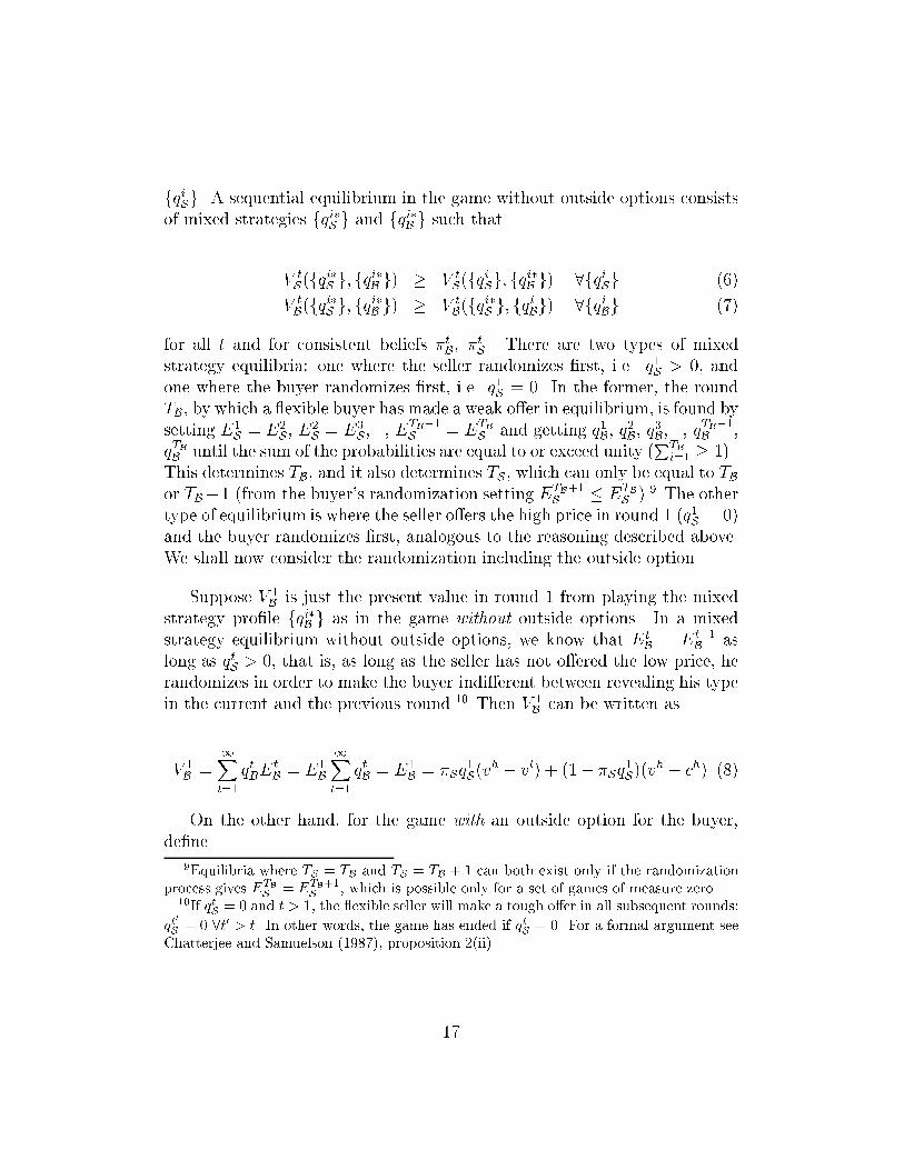
fqiSg. A sequential equilibrium in the game without outside options consists

of mixed strategies fqi�Sg and fqi�

Bg such that

V tS(fqi�

Sg; fqi�

Bg) � V t

S(fqi

Sg; fqi�

Bg) 8fqi

Sg (6)

V tB(fqi�

Sg; fqi�

Bg) � V t

B(fqi�

Sg; fqi

Bg) 8fqi

Bg (7)

for all t and for consistent beliefs �tB, �t

S. There are two types of mixed

strategy equilibria: one where the seller randomizes �rst, i.e. q1S> 0, and

one where the buyer randomizes �rst, i.e. q1S= 0. In the former, the round

TB, by which a exible buyer has made a weak o�er in equilibrium, is found bysetting E1

S= E2

S, E2

S= E3

S,..., ETB�1

S= E

TBS

and getting q1B, q2

B, q3

B,..., qTB�1

B,

qTBB

until the sum of the probabilities are equal to or exceed unity (PTB

i=1 � 1) .This determines TB, and it also determines TS , which can only be equal to TBor TB+1 (from the buyer's randomization setting ETB+1

S� E

TBS).9 The other

type of equilibrium is where the seller o�ers the high price in round 1 (q1S= 0)

and the buyer randomizes �rst, analogous to the reasoning described above.We shall now consider the randomization including the outside option.

Suppose V 1Bis just the present value in round 1 from playing the mixed

strategy pro�le fqi�Bg as in the game without outside options. In a mixed

strategy equilibrium without outside options, we know that EtB= Et�1

Bas

long as qtS> 0, that is, as long as the seller has not o�ered the low price, he

randomizes in order to make the buyer indi�erent between revealing his typein the current and the previous round.10 Then V 1

Bcan be written as

V 1B=

1Xt=1

qtBEtB= E1

B

1Xt=1

qtB= E1

B= �Sq

1S(vh � vl) + (1� �Sq

1S)(vh � ch) (8)

On the other hand, for the game with an outside option for the buyer,de�ne

9Equilibria where TS = TB and TS = TB + 1 can both exist only if the randomizationprocess gives ETB

S= ETB+1

S, which is possible only for a set of games of measure zero.

10If qtS= 0 and t > 1, the exible seller will make a tough o�er in all subsequent rounds:

qt0

S= 0 8t0 > t. In other words, the game has ended if qt

S= 0. For a formal argument see

Chatterjee and Samuelson (1987), proposition 2(ii).

17

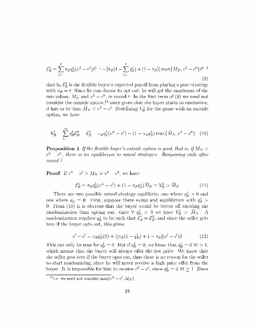
E tB=

tXi=1

�SqiS(vh� vl)�i�1+ [�S(1�

tXi=1

qiS)+ (1��S)]maxf �MN ; v

h� chg�t�1

(9)that is, E t

Bis the exible buyer's expected payo� from playing a pure strategy

with nB = t. Since he can choose to opt out, he will get the maximum of thetwo values, �MN and vh � ch, in round t. In the �rst term of (9) we need notconsider the outside option,11 since given that the buyer starts to randomize,it has to be that �MN < vh� vl. Rede�ning V 1

Bfor the game with an outside

option, we have

V1B=

1Xt=1

qtBE tB= E1

B= �Sq

1S(v

h � vl) + (1� �Sq1S)maxf �MN ; v

h � chg (10)

Proposition 1 If the exible buyer's outside option is good, that is, if �MN >

vh � ch, there is no equilibrium in mixed strategies. Bargaining ends after

round 1.

Proof. If vh � vl > �MN > vh � ch, we have

E1B= �Sq

1S(vh � vl) + (1� �Sq

1S) �MN = V1

B> �MN (11)

There are two possible mixed strategy equilibria: one where q1S> 0 and

one where q1S= 0. First, suppose there exists and equilibrium with q1

S>

0. From (10) it is obvious that the buyer would be better o� entering therandomization than opting out, since 8 q1

S> 0 we have V1

B> �MN . A

randomization requires q1Bto be such that E1

S= E2

S, and since the seller gets

zero if the buyer opts out, this gives:

vl � cl = �Bq1B(0) + [(�B(1� q1B) + 1� �B](v

l � cl)� (12)

This can only be true for q1B= 0. But if q1

B= 0, we know that qt

B= 0 8t > 1,

which means that the buyer will always o�er the low price. We know thatthe seller gets zero if the buyer opts out, thus there is no reason for the sellerto start randomizing, since he will never receive a high price o�er from thebuyer. It is impossible for him to receive ch � cl, since qt

B= 0 8t � 1. Since

11i.e. we need not consider maxfvh � vl; �MNg

18

the only o�er that the buyer will accept from the seller is vl and delay iscostly, the exible seller can do no better than reveal his type in round 1 ando�er the low price. The outside option makes it possible for the buyer toreceive the full gains from trade in the �rst round, even though the seller hasa relatively high probability that the buyer is exible. The option to choose�MN > vh � ch makes trade instantaneous and favorable for the buyer.

Now, suppose there exists an equilibrium in mixed strategies with q1S= 0.

This means that the buyer would start to randomize in round 1, and hisexpected payo� from randomizing would be

V1B=

1Xt=1

qtBEtB= E1

B= �MN (13)

In other words, the buyer would have to be indi�erent in each roundbetween choosing �MN and continuing the randomization, with an expectedpayo� of �MN . The seller, on the other hand, can get at most vl � ch byrevealing his type, since otherwise the buyer opts out, leaving him with apayo� of zero. Again, the seller would prefer to get vl � ch as early aspossible, since delay is costly. Therefore, it cannot be an equilibrium whereqtS= 0 for any t. The seller reveals his type in round 1 even though he has

a relatively high prior that the buyer is exible. We conclude that a goodoutside option eliminates the mixed strategy equilibrium. 2

Proposition 2 In equilibrium, the exible buyer never takes the outside op-

tion in any round t > 1.

Proof. Suppose the outside option �MN is not taken in round 1. For thisto be the case, it must be that �MN is less than the exible buyer's expectedvalue in round 1 from the remainder of the game, V 1

B. To �nd the equilibrium

strategies, �rst suppose that �MN < vh� ch. This implies that V1B= V 1

B, and

we have

V1B= �Sq

1S(vh � vl) + (1� �Sq

1S)(vh � ch) = E1

B> �MN (14)

Then we know from �MN < E1Bthat �MN < E t

Bfor any t > 1 as long as the

buyer randomizes (qtB> 0), since E t

B= E t�1

Bis precisely the condition to make

the buyer indi�erent between stopping and continuing the randomization.But then the outside option is never taken. The randomizing strategies are

19

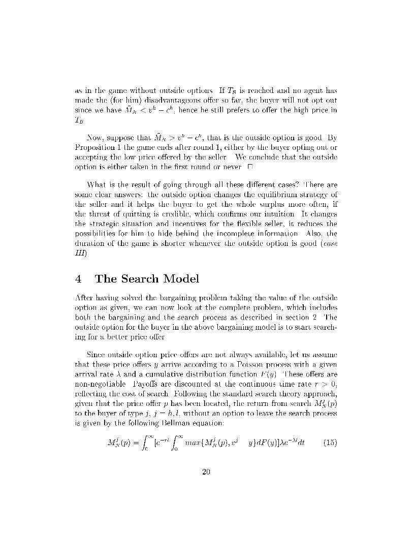
as in the game without outside options. If TB is reached and no agent hasmade the (for him) disadvantageous o�er so far, the buyer will not opt outsince we have �MN < vh � ch, hence he still prefers to o�er the high price inTB.

Now, suppose that �MN > vh � ch, that is the outside option is good. ByProposition 1 the game ends after round 1, either by the buyer opting out oraccepting the low price o�ered by the seller . We conclude that the outsideoption is either taken in the �rst round or never. 2

What is the result of going through all these di�erent cases? There aresome clear answers: the outside option changes the equilibrium strategy ofthe seller and it helps the buyer to get the whole surplus more often, ifthe threat of quitting is credible, which con�rms our intuition. It changesthe strategic situation and incentives for the exible seller, it reduces thepossibilities for him to hide behind the incomplete information. Also, theduration of the game is shorter whenever the outside option is good (caseIII).

4 The Search Model

After having solved the bargaining problem taking the value of the outsideoption as given, we can now look at the complete problem, which includesboth the bargaining and the search process as described in section 2. Theoutside option for the buyer in the above bargaining model is to start search-ing for a better price o�er.

Since outside option price o�ers are not always available, let us assumethat these price o�ers y arrive according to a Poisson process with a givenarrival rate � and a cumulative distribution function F (y). These o�ers arenon-negotiable. Payo�s are discounted at the continuous time rate r > 0,re ecting the cost of search. Following the standard search theory approach,given that the price o�er p has been located, the return from search M

jN (p)

to the buyer of type j, j = h; l, without an option to leave the search processis given by the following Bellman equation:

MjN(p) =

Z1

0

[e�rtZ1

0

maxfM jN (p); v

j � ygdF (y)]�e��tdt (15)

20

since the probability of receiving exactly one o�er when price o�ers come froma Poisson distribution is �e��.12 Thus, when the �rst o�er y arrives at timet, the optimal search policy would be to choose the higher expected payo�resulting from the following two choices: accepting o�er y and receiving thepayo� vj � y or continuing the search with a payo� of M j

N , where the latteris again his value function given by (15).

In order to solve the complete bargaining-search game as given in Figure1, the results from the previous section for the bargaining problem with two-sided incomplete information with a given outside option for the buyer willbe used. When G denotes the subgame starting at the bargaining phase,and N denotes the subgame starting at the search phase, let MG be themaximum equilibrium payo� to the buyer from the subgame G and MN bethe maximum equilibrium payo� to the buyer from the subgame N . We willallow for the buyer to return to the bargaining table once he started search,and we will see if this option of returning to the old bargaining partner is evertaken in this game with incomplete information. As Muthoo (1995) showsfor a split-the-pie game with complete information, in equilibrium, a playerwill never choose to return to the bargaining table if he has an outside optionto search for better o�er.

We will approach the solution by going through the three cases of section2.2, which describe the bargaining equilibrium that is de�ned by the proba-bilities �S and �B relative to ��S and ��B. Following Baucells and Lippmann(1999), we will distinguish two regimes: First, we consider the case wherethe expected return from search is used as an outside option. In the secondregime, the buyer will have to use actual o�ers to negotiate with the seller.It will be shown that this has an important impact for the solution of thegame.

12If k is the number of o�ers received, then the probability fP (k + 1;�) = fP (k;�)�

k+1.

Since for k = 0, fP (0;�) = e��, we have fP (1;�) = �e��, and the expected time for the�rst o�er is

R10

�e��tdt.

21

4.1 Regime I: Symmetric Information about the Out-

side Option

case I: �B < ��B

The solution of the complete bargaining-search game will always dependon the value of the outside option. If there is symmetric information aboutthe outside option, we assume that the Seller and the Buyer know the pa-rameters of the distribution of the outside o�ers. Then the buyer can usehis expected value from search as his outside option and we have �B < ��B,we know from case I of the bargaining equilibrium that the exible seller'soptimal strategy is to reveal his type immediately, irrespective of the valueof the outside option. Then

MG = maxfvh � vl;MNg (16)

When B follows an optimal search policy, the value of the outside optionMN , i.e., the maximum expected payo� for the game starting at N , is foundby applying the techniques of dynamic programming. Bellman's equation is

MN =Z1

0

[e�rtZ1

0

maxf�MG;MN ; vh � ygdF (y)]�e��tdt (17)

since, according to the game structure of Figure 1, we leave the buyer thechoice to go back to bargain with the seller after he started the search. Weassume that this will take � units of time, therefore payo�s from the gamestarting again at G at time t + � are discounted by �. The solution to thebargaining part as given in (16). To solve (16) and (17) simultaneously, �rstsuppose that �MG > MN . If this is the case, then it must be that

MG = maxfvh � vl;MNg = vh � vl (18)

since otherwise we would have �MG = �MN < MN , which contradicts ourassumption. Knowing that the seller cannot o�er a lower price than vl, thebest that the buyer can get from returning to bargaining is again vh � vl,but now discounted by the amount of time he spent searching and the costof returning to the bargaining table. Will the buyer ever go back to bargainwith the seller once he started the search? In order to have an incentive todo this, it must be that

22

MN =Z1

0

[e�rtZ1

0

maxf�MG;MN ; (vh � y)gdF (y)]�e��tdt

=Z1

0

[e�rtZ1

0

maxf�MG; (vh � y)gdF (y)]�e��tdt (19)

that is, �MG > MN . But if this is true, then also MG > MN . And sinceMG = maxfvh� vl;MNg, it must be that MG = vh� vl. But then the buyerwould never start the search. Thus, as long as the seller o�ers vl irrespectiveof the value of the outside option (which is always true in case I), the buyerwill, in equilibrium, never go back to bargain with the seller once he choseto start the search.

Then MN is reduced to

MN =Z1

0

[e�rtZ1

0

maxfMN ; vh � ygdF (y)]�e��tdt (20)

since we know that going back to the bargaining table is not included in theoptimal path. When p is the \o�er in hand", i.e. the currently availableprice o�er, the return from search is

MN =Z1

0

e�rt[MN

Z1

pdF (y) +

Z p

0

(vh � y)dF (y)]�e��tdt (21)

which can be simpli�ed to

MN =�

r + �[MN (1� F (p)) +

Z p

0

(vh � y)dF (y)] (22)

We are looking for an optimal reservation price, p�, that makes the buyerindi�erent between accepting and continuing search for one more round. Re-arranging (22), we get

MN = vh � p =

R p0 (v

h � y)dF (y)r�+ F (p)

(23)

Following the arguments of standard search theory, e.g. Lippman andMcCall (1976), there is a unique optimal reservation price, p�, that solvesthe above equation. Then the optimal search policy given that the buyer isin subgame N is to

- stop search if p � p� and

23

- continue search if p > p�, where p� is the solution to

vh � p� =

R p�0 (vh � y)dF (y)

r�+ F (p�)

(24)

This implies that the maximum payo� for the buyer in the complete search-bargaining game is

MG = maxfMN ; vh � vlg = maxfvh � p�; vh � vlg (25)

The optimal strategy for a exible buyer in the bargaining-search gameis

� if p� < vl, with p� given by (24), then a exible buyer should opt out,i.e. start search. Following the optimal search policy, he should stopthe search if he �nds a price o�er p � p� and he should continue tosearch as long as he receives o�ers p > p�.

� if p� > vl then the game ends in the bargaining phase in the �rst round.The buyer accepts the exible seller's o�er vl. There is no search inthis case.

case II: �B > ��B and �S < ��S

In section 3.2 describing the bargaining equilibrium we found that, unlikecase I, in case II the seller's strategy depends on the outside option for thebuyer. If it is \good", the exible seller will o�er vl and the buyer gets thehigh surplus, while if it is \bad", he will o�er ch and get the highest possiblesurplus himself. Thus MG is not known if MN is not known. In orderto determine MN , the value of the outside option, we set up the Bellmanequation again:

MN =Z1

0

e�rt[Z1

0

maxf�MG;MN ; vh � ygdF (y)]�e��tdt

The seller will reveal his type as a exible agent if the buyer's outsideoption is \good", that is, if MN > vh � ch and the buyer's maximum payo�from the game starting in the bargaining phase G is

MG = maxfvh � vl;MNg

24

as in (16), whereas if the outside option is \bad", that is MN < vh � ch,the exible seller will o�er only ch and the maximum payo� from the gamestarting in G is

MG = maxfvh � ch;MNg = vh � ch

The di�erence to case I is that here, in case II, it seems that the buyermight have an incentive to come back to the bargaining table if he could lo-cate an outside o�er lower than ch, but higher than vl, which would persuadethe exible seller to o�er him vl when he comes back. Suppose, then, that�MG > MN , i.e., the buyer prefers to return to the bargaining table ratherthan to continue search. But in order for the buyer to have opted out, it mustbe that the expected value of search, MN , is greater than his surplus fromthe seller's current o�er in the �rst bargaining round, vh�ch. In other words,the buyer has a good outside option. But then the exible seller changes hisstrategy from o�ering ch to o�ering vl in round 1 of the bargaining phase,since if MN > vh� ch, the buyer would search until he locates a price that isless or equal to his optimal reservation price, which must be lower than ch.This would give the seller a payo� of zero, thus he prefers to o�er vl in round1. Again, in equilibrium, �MG > MN implies that MG > MN and there isno search.

However, a this point, neither MG nor MN are known, thus it seemsthat we do not know when the no-search strategy applies. But the onlypossibility that search is optimal for the buyer is when �MG < MN . Theoptimal reservation price is then given by (24), which only depends on thesearch parameters. Then the optimal search policy for the game starting atN is to start search if vh � p� > �MG = �(vh � vl) or p� < vh(1 � �) + �vl,since otherwise it cannot be that MN > MG, and to continue search as longas the price o�er p > p�. Whenever the current o�er p < p�, the buyershould accept the o�er. His expected payo� from search, i.e. the expectedpayo� from the game starting in N following the optimal search policy, isvh � p�. If p� is known, MN = vh � p� is known and therefore the completebargaining-search game starting at MG can be solved:

� if p� < ch, which we call a \good" outside option, then the highestpossible payo� the buyer can get is

MG = maxfvh � vl; vh � p�g

25

since the good outside option implies that the exible seller, knowingthat this is the only o�er that ensures that the buyer possibly acceptsthe deal with him, will o�er vl. Then the buyer will start the search (ifand) only if p� < vl, which makes the above condition p� � vh(1� �)+�vl redundant. If ch > p� > vl then the buyer will choose to accept theseller's o�er vl.

� If the outside option is bad, that is, if p� > ch, then the buyer is leftwith the low surplus vh � ch from bargaining with the seller, there isno search in this case.

Again, the option to return to the bargaining table is never taken inequilibrium, since search is only started if p� < vl, and the buyer has noincentive to go back to the seller once he started search. Comparing case II

to case I, as long as �S < ��S and p� < ch, the seller's prior probability for thebuyer being exible is irrelevant. He will o�er vl if he is exible. Only if theoptimal reservation price is higher that the seller's tough o�er, it will dependon �B what the seller's strategy is and to which agent the high surplus goes.

case III: �B > ��B and �S > ��S

Looking at case III of the bargaining equilibrium where �B > ��B and�S > ��S , we found that there is an equilibrium in mixed strategies if theoutside option is bad and in pure strategies where the seller o�ers vl in round1 if the outside option is good. The question is again, when do we know thatthe outside option is good (which is decisive for the solution of the game),since MN is also depending on MG. The value of the outside option is againgiven by (17). We proceed in an analogous way to the cases before. To �ndthe optimal strategies for the bargaining-search game, suppose �MG > MN .Can there be an incentive for the buyer to return to the bargaining tableafter he started search? The argument is analogous to the previous cases:If the outside option is good, the seller o�ers vl in round 1 and we haveMG = maxfvh � vl;MNg = vh � vl. There is no search in this case. Ifthe outside option is bad, MG = maxfV1

B;MNg, where V1B is the buyer's

expected payo� from the mixed strategy equilibrium as described in theprevious section. Using our assumption �MG > MN , we have MG = V1

B andthe buyer does not search.

To complete the case, if �MG �MN , we have �MG = �maxfvh�vl;MNgwith a good outside option and �MG = �(vh� ch) with a bad outside option.

26

The latter implies no search if p� > ch, while for the former, p� is as de�nedin (24).

The analysis of the bargaining-search game leads to the following conclu-sions: For all possible values of �B, �S , ��B, ��S , which de�ne the bargainingequilibrium, there is one optimal reservation price for the game starting atN , which depends only on the distribution of the incoming o�ers F(y), thearrival rate � and the discount rate r. Using the expected return from searchas a valid outside option implies that the option of returning to the bar-gaining table after having started search is redundant, which coincides withMuthoo's (1995) result for a bargaining and search game with complete in-formation. The move-structure of the game remains stationary. Since thismeans that once search is started the buyer remains in the search process,the optimal reservation price does not depend on what the seller can o�er.The decision whether to start search is made by �rst comparing p� to ch inorder to �nd out if the outside option is \good" or \bad" (except for case I,where the exible seller always o�ers vl). In the end, search is only startedif p� < vl, but never to induce the bargaining partner to o�er a lower price.

4.2 Regime II: Asymmetric Information about the Out-

side Option

Using the expected return from search a valid outside option, the previoussection showed that the bargaining-search game is stationary in its structure.This is exactly the reason for the result that it is never optimal to return tothe bargaining table once search is started. In equilibrium, agents in bothgames with complete and incomplete information should not be searchingwith the intention to go back to bargaining. This result is somewhat surpris-ing, given the fact that one might also think about improving the bargainingposition when opting out, and not necessarily about leaving the bargainingpartner forever. But in Regime I the buyer opts out without ever returning,which makes a game with the option to return to the old bargaining partneridentical to one without such option.

The key of this result lies in the stationary structure of the bargaining-search game. The seller's equilibrium strategy in the subgame G does notchange after the buyer has opted out. This, on the other hand, is explainedby what was considered a \valid" outside option in the previous section:

27

the expected value of search. This value is at the same time the incentivefor the buyer to start the search process and his threat for the seller. Nowsuppose that the seller does not have any information about the distributionof the buyer's outside option. This can happen if the buyer cannot crediblycommunicate his information about the search parameters. The buyer thenhas to use an actual o�er as a valid outside option. This can be particularlyrelevant in a job search situation, where a currently employed worker, whoprefers to stay with his employer but wants a raise in his salary, has to bringan actual o�er from another employer in order to have a credible outsideoption.

This changes the structure of the bargaining-search game. Intuitively,it should be worth for the buyer now to come back to the bargaining tablewith an actual o�er in order to receive a better price from the seller he wasbargaining with earlier, as long as that price the seller can o�er him is stillbetter than the actual outside o�er or the expected value of search. Thissection will show that there is an equilibrium where B searches for some timeand returns to bargaining, if actual o�ers only can be used as a valid outsideoption.

Let Y be the realization of the random variable, in other words Y shalldenote an actual outside o�er located by the buyer after he opted out. Abuyer will have an incentive to opt out, if the highest payo� he can getfrom the game starting at N is higher than accepting the seller's o�er. Theexpected value from the game starting at N is now de�ned as

MN =Z1

0

e�rt[Z1

0

maxf�M tG;MN ; v

h � ygdF (y)] (26)

with M tG denoting the expected maximum payo� the buyer can receive from

the subgame starting at MG after he searched for t time units. We will showthat the bargaining subgames are not identical anymore, hence the timeindex. We will approach the solution of this game similarly to the previousone, i.e. go through the three cases of the bargaining equilibrium in order to�nd a solution for the complete bargaining-search game.

case I

From regime I we can see that case I is trivial as far as the treatmentof the outside option is concerned. Irrespective of the value of the outside

28

option the equilibrium strategy for the seller is to o�er vl and hence the buyerwill only opt out if p� < vl. In Regime II where he has to use actual o�ers,this will not change, since the seller's equilibrium strategy will not changeover time, hence M t

G =MG.

case II

This case is more interesting, since here we have a bargaining equilibriumwhere in the game without outside options both seller types o�er the sameprice, vh, and the buyer cannot identify a exible seller in round 1. As shownin the previous section, only a good outside option changes the exible seller'sequilibrium strategy to o�ering vl. However, if only actual o�ers can be usedas a credible threat, the buyer would �rst have to start search in order tolocate an o�er. He will opt out if the expected discounted value from search,including the option to go back to bargaining, is higher than vh� ch, the lowpayo� from bargaining that he is o�ered in the �rst round in case II. MN

is as given in (26), and we have to determine M tG, the expected maximum

payo� from returning to bargaining considering the probability of �nding ano�er better than ch at time t when the �rst outside o�er has been located.

M tG = maxfMN ; (1 � �S)(v

h � ch) +

�S [(1� F (ch))(vh � ch) + F (ch)(vh � vl)]g(27)

To solve (26) with M tG as given in (27), suppose �rst that �M t

G > MN .Then we know that the expected surplus from returning to the (unknowntype of) seller is

M tG = (1� �S)(v

h � ch) + �S [(1� F (ch))(vh � ch) + F (ch)(vh � vl)]

= vh � ch + �SF (ch)(ch � vl) (28)

and the highest possible price �p that would be acceptable from search is thengiven by

vh � �p = �M tG = �[vh � ch + �SF (c

h)(ch � vl)]

�p = vh(1� �) + �[ch � �SF (ch)(ch � vl)] (29)

29

Then the expected return from search is

MN =�

r + �

Z1

0

maxf�M tG; v

h � ygdF (y)

=�

r + �[Z �p

0

(vh � y)dF (y) + (1� F (�p))(vh � �p)] (30)

To proceed, we will use the following result from standard search theory,which states some properties of the payo� function MN(�):

Lemma 1 If the expected payo� the buyer can achieve by following anoptimal search policy is

MN (p) =�

r + �[Z p

0

(vh � y)dF (y) + (1� F (p))MN (p)]

Then the payo� function MN(�) has the following properties:(1) vh � p� =M(p�)(2) p� < p <1)M(p) > vh � p

(3) 0 < p < p� )M(p) < vh � p

Then since (30) is true given our assumptionMN < �M tG, orMN < vh��p,

using Lemma 1 we can conclude that

MN(�p) =�

r + �[Z �p

0

(vh � y)dF (y) + (1� F (�p)(vh � �p)] < vh � �p (31)

if and only if �p < p�.

Now suppose that �M tG < MN to complete the solution of (26) . In

expectation, the buyer won't go back to the seller, but follow his optimalsearch policy giving him an optimal reservation price p�. In this case wehave

MN =�

r + �

Z1

0

maxfMN ; vh � y)dF (y) (32)

and p� is given again by (24). The return from search is MN = vh � p�,which is independent of the bargaining parameters. Again, this is true if�M t

G < MN = vh � p�. Now �M tG < MN implies that

30

�[vh � ch + F (ch)(ch � vl)(1� �S)] < MN = vh � p� (33)

where the LHS is just a linear combination of vh � ch and vh � vl. Now weput the complete solution together:

The �rst assumption, �M tG > MN is possible i�

vh � p� < �M tG (34)

orp� > �p (35)

whereas the second assumption, �M tG < MN is possible i�

�M tG < vh � p� (36)

or

p� < �p (37)

This shows that there is a unique solution. We conclude that the condi-tions and hence the motivation to start search and the condition to continue

search di�er: The buyer opts out in case II as long as ch > �p. Then two casesare possible: Either p� > �p, which means the buyer will (in expectation) re-turn to the bargaining table and he just uses the outside option to locate ano�er in order to renegotiate with the seller make the seller change his o�er.Or, p� < �p, which means that the buyer will continue search according to hisoptimal search policy.

case III

Using actual o�ers as an outside option, the seller has no incentive hereto o�er the low price vl. Thus, we have to compare the expected valuefrom playing the mixed strategy in the bargaining game to the expectedreturn from search in order to see when the buyer opts out, that is, checkif MN > V1

B. To determine the value of MN , we use the result of case II:�M t

G > MN i� �p < p�, and thus the buyer will opt out if �M tG > V1

B, or

�[(vh � ch)(1� �SF (ch)) + (vh � vl)�SF (c

h)] >

(vh � vl)�Sq1S + (vh � ch)(1� �Sq

1S) (38)

31

which just says that the buyer should opt out if the probability of locatinga price o�er lower than ch (considering discounting) is higher than the prob-ability that the seller o�ers the low price vl in the �rst round in his mixedstrategy. He will return to renegotiate with the seller after locating the �rstoutside o�er and in expectation, the exible seller will o�er him the low pricewhen he returns. Again, the outside option is chosen in order to change theseller's optimal strategy, not because the expected return from search is high.

On the other hand, �M tG < MN i� �p > p�, and then the buyer will opt

out if

vh � p� > V1B = (vh � ch)(1� �Sq

1S) + (vh � vl)�Sq

1S (39)

p� < ch + �Sq1S(c

h � vl) (40)

and using Proposition 1, we conclude that the buyer will never return to thebargaining table. The mixed strategy equilibrium remains a solution to thebargaining-search problem if p� > ch + �Sq

1S(c

h � vl).

What is di�erent from the result of Regime I? When expected o�ers are avalid outside option, for any �B and �S , an optimal reservation price p� < ch

induces the exible seller to o�er the low price vl in the �rst round, and unlessthe reservation price from search is not too low (p� > vl), the buyer doesn'topt out. There will not be a renegotiation in equilibrium under Regime I. InRegime II, where actual o�ers have to be used as a valid outside option, thebuyer actually will opt out and start to search if the seller thinks he is likelyto be exible (�B > ��B). In expectation, he will go back to the bargainingtable after locating the �rst outside o�er if p� > �p, since the expected pricehe will have to pay to the seller after renegotiating is lower than the optimalreservation price from search. The outside o�er might or might not help himto renegotiate, this depends on the realization of the located price, which isa random variable in this model.

Notice that under Regime II it is possible that the buyer searches for morethan one outside o�er and then returns to the bargaining table. This happenswhen the realization of the �rst price o�er located through search is notsu�ciently low to induce the exible seller to o�er vl when they renegotiate.The buyer will then continue search until he locates an o�er Y such thatvh � Y < �(vh � ch), or Y < vh(1 � �) + �ch. He will still return to the

32

bargaining table as long as the reservation price from search, p� is higherthan the expected price �p he will have to pay the seller.

5 Conclusion

This paper studies a noncooperative bargaining model between a buyer and aseller, where both agents have incomplete information about the opponent'svaluation for the good to be traded, and where the buyer's outside option isto buy via search. The model interlaces a standard sequential search processand a version of Rubinstein's alternating-o�ers bargaining process.

First, the bargaining process with two-sided incomplete information isanalyzed, taking the outside option as given. Incorporating the results ofthe bargaining process in the complete bargaining-search game, we solve forthe optimal bargaining and search strategies when the outside option for thebuyer consists of searching for a better price o�er, and when the buyer canchoose to return to bargaining with the seller once he started search. Twodi�erent regimes for the search process are distinguished:

� Regime I: Symmetric information about the outside option, i.e. theexpected return from search can be used as a credible outside optionand

� Regime II: Asymmetric information about the outside option, i.e. thebuyer has to use actual o�ers to (re)negotiate with the seller.

As shown in the paper, this distinction has an important impact on thesolution of the bargaining-search game. In Regime I, the condition to optout depends on the optimal reservation price, which is a function only of thedistribution parameters of the outside o�ers and the discount rate, but noton the bargaining parameters, in particular not on the seller's o�er. Theoption to return to the bargaining table is redundant, which coincides withMuthoo's (1995) result for a game with complete information. Thus, searchis never started to induce the bargaining partner to o�er a lower price, butwith the intention to follow the optimal stopping rule as in a pure searchprocess.

In Regime II, when actual outside o�ers have to be used as the outsideoption in the bargaining process, the stationarity of the move-structure of

33

the game is not preserved and hence, a renegotiation with the old bargainingpartner is possible in equilibrium. An important result is that the conditionswhen to start search and when to continue search di�er. The unique solutiondetermines whether the buyer opts out in order to locate an outside o�erand to use it for renegotiation with the seller, or whether the buyer opts outwith the intention to continue search according to the optimal search policewithout ever returning to the seller.

This model is a basic framework for a larger variety of bargaining-searchproblems. It is easy to think about other regimes that would be worth consid-eration in a similar setting, for example if the player without outside optionis available only temporarily. Another extension would be a situation wherethe player with the outside option is incompletely informed about the distri-bution function of outside o�ers. In this case, search would involve learningand the equilibrium strategies would be non-stationary. These considera-tions could be particularly useful in e-commerce using programmed biddingagents, when incoming information cannot be processed fast enough and/orstrategies are too complex for human traders.

[]

References

[1] M.A. Arnold and S.A. Lippman. Posted prices versus bargaining inmarkets with asymmetric information. Economic Inquiry, XXXVI:450{457, 1998.

[2] M. Baucells and S.A. Lippman. Bargaining with search as an out-side option: The impact of the buyer's future availability. Unpub-lished Manuscript, The Anderson Graduate School of Business, UCLA,September 1999.

[3] H. Bester. Bargaining, search cost and equilibrium price distributions.Review of Economic Studies, LV:201{214, 1988.

[4] K. Binmore. Bargaining and coalitions. In A. Roth, editor, Game-

Theoretic Models of Bargaining, pages 269{304. Cambridge UniversityPress, 1985.

34

[5] K. Chatterjee and L.Samuelson. Bargaining with two-sided incompleteinformation: An in�nite horizon model with alternating o�ers. Review

of Economic Studies, LIV:175{192, 1987.

[6] K. Chatterjee and L.Samuelson. Bargaining under two-sided incompleteinformation: The unrestricted o�ers case. Operations Research, 36:605{618, 1988.

[7] P. Diamond and E. Maskin. An equilibrium analysis of search and breachof contract, i: Steady states. Bell Journal of Economics, 10:282{316,1979.

[8] D. Fudenberg and J.Tirole. Sequential bargaining under incompleteinformation. Review os Economic Studies, 50:221{248, 1983.

[9] S.A. Lippman and J.J.McCall. The economics of job search: A survey.Economic Inquiry, XIV:155{189, 1976.

[10] S.A. Lippman and J.J.McCall. The economics of uncertainty: Selectedtopics and probabilistic methods. In K.J. Arrow and M.Intriligator,editors, Handbook of Mathematical Economics, chapter 6. North-HollandPublishing Company, Amsterdam, 1981.

[11] D.T. Mortensen. The matching process as a noncooperative bargain-ing game. In J.J. McCall, editor, The Economics of Information and

Uncertainty, chapter 7. The University of Chicago Press, 1982.

[12] A. Muthoo. On the strategic role of outside options in bilateral bargain-ing. Operations Research, 43(2):292{297, 1995.

[13] A. Rubinstein. Perfect equilibrium in a bargaining model. Econometrica,50:97{108, 1982.

[14] A. Rubinstein. A bargaining model under incomplete information.Econometrica, 53:1151{1172, 1985.

[15] A. Rubinstein and A. Wolinsky. Equilibrium in a market with sequentialbargaining. Econometrica, 53:1133{1150, 1985.

[16] A. Shaked and J.Sutton. Involuntary unemployment as a perfect equi-librium in a bargaining model. Econometrica, 52:1351{1364, 1984.

35