banks interconnectivity and leverage · 2015-10-26 · .35.4.45.5.55 interconnectivity 2000 2005...
TRANSCRIPT

Banks Interconnectivity and Leverage∗
Alessandro BarattieriCollegio Carlo Alberto and ESG UQAM
Laura MorettiCentral Bank of Ireland
Vincenzo QuadriniUniversity of Southern California
18 September 2015
VERY PRELIMINARY AND INCOMPLETECOMMENTS WELCOME
Abstract
In this paper we document that in the period that preceded the 2008 crisis, financialfirms have become more interconnected (with each other) and more leveraged. To un-derstand how cross-bank interconnectivity is related to bank leverage we first developa dynamic model where banks make risky investments in the nonfinancial sector. Toreduce the idiosyncratic risk, they sell some of the investments to other banks (inter-connectivity). Thanks to diversification, the portfolio of each bank becomes less riskywhich increases the incentive to leverage. We explore this mechanism empirically usinga large sample of over 14,000 financial institutions from 32 OECD countries along threedimensions: across banks, time and countries. Along each of these dimensions we findthat there is a strong positive association between banks interconnectivity and leverage.In particular, banks that are more financially interconnected are also more leveraged;when an individual bank becomes more connected it raises its leverage; countries inwhich the banking sector is more interconnected tend to have more leveraged banks.Although bank interconnectivity reduces the idiosyncratic risk faced by each bank, itdoes not eliminate the aggregate financial risk which could increase with the leverageof whole financial sector.
JEL classification:Keywords: Interconnectivity, Leverage
∗The views expressed in this paper do not reflect the views of the Central Bank of Ireland or the EuropeanSystem of Central Banks. All errors are ours.
1

1 Introduction
During the last three decades we have witnessed a significant expansion of the financial
sector. As shown in Figure 1, the assets of US financial businesses have more than doubled
as a fraction of the country GDP. This trend has been associated to two other trends within
the financial sector. First, in the period that preceded the 2008 crisis, financial intermediaries
have become more interconnected, that is, they have increased the holding of liabilities issued
by other financial intermediaries. Second, financial firms have become more leveraged.
0%
100%
200%
300%
400%
500%
600%
1965 1970 1975 1980 1985 1990 1995 2000 2005 2010
Assets of the US financial sector (Percent of total GDP)
Figure 1: The growth of the financial sector.
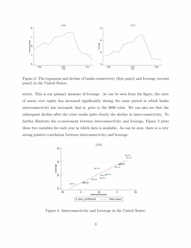
To illustrate these two trends, the first panel of Figure 2 plots the ratio of non-core
liabilities over total assets for the US banking sector using data from Bankscope, for the
period 1999-2011. Non-core liabilities are those issued to other banks while core liabilities are
issued to nonfinancial sectors (like the typical bank deposits of households and nonfinancial
businesses). A more detailed description of the data will be provided later in the empirical
section of the paper. We interpret the ratio as an index of financial inter-connectivity among
banks. As can be seen from the figure, this ratio has increased significantly prior to the 2008
financial crisis.
The second panel of Figure 2 plots the ratio of assets over equity for the US banking
2
.35
.4.4
5.5
.55
Inte
rcon
nect
ivity
2000 2005 2010Year
USA
1520
2530
Leve
rage
2000 2005 2010Year
USA
Figure 2: The expansion and decline of banks connectivity (first panel) and leverage (secondpanel) in the United States.
sector. This is our primary measure of leverage. As can be seen from the figure, the ratio
of assets over equity has increased significantly during the same period in which banks
interconnectivity has increased, that is, prior to the 2008 crisis. We can also see that the
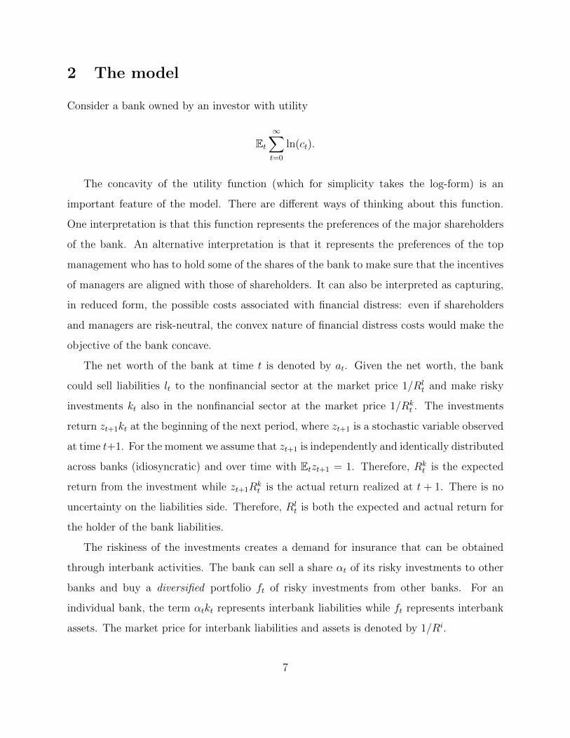
subsequent decline after the crisis tracks quite closely the decline in inter-connectivity. To
further illustrate the co-movement between interconnectivity and leverage, Figure 3 plots
these two variables for each year in which data is available. As can be seen, there is a very
strong positive correlation between interconnectivity and leverage.
19992000
20012002
2003
20042005
20062007
2008
200920102011
1520
2530
Leve
rage
.35 .4 .45 .5 .55Interconnectivity
WAV_LEVERAGE Fitted values
USA
Figure 3: Interconnectivity and Leverage in the United States.
3

Motivated by these empirical patterns, this paper addresses two questions. First, are the
simultaneous increases (and subsequent declines) in inter-connectivity and leverage related?
Second, what are the forces that have induced banks to become more interconnected and
leveraged?
To address these questions we first develop a dynamic model where banks make risky
investments outside the financial sector. To reduce the idiosyncratic risk, banks sell some of
the investments to other banks and become more diversified. Because of the diversification,
they are willing to invest more and take more leverage.
To investigate this mechanism empirically, in the second part of the paper we use data
from Bankscope and explore the prediction of the model along three dimensions: across
banks, across time and across countries. The empirical analysis suggests that there is a
strong association between banks interconnectivity and leverage. In particular, banks that
are more financially interconnected are more leveraged; when an individual bank becomes
more connected to other banks, it also raises its leverage; countries in which the banking
sector is more connected tend to have more leveraged banks. Although this does not test the
specific mechanism that in the model generates the positive association between connectivity
and leverage, it is consistent with it.
A second prediction of the model is that bank connectivity and leverage increase when the
cost of diversification declines and/or the difference between the investment return and the
cost of funds (return spread) increases. This provides two possible candidates for explaining
the pre-crisis increase in connectivity and leverage: (i) an increase in the operating margin
of banks; and/or (ii) a decline in the cost of diversification (resulting, for example, from
financial innovations).
The two potential changes have different implications for the return differential between
the investments and the liabilities of banks. If the change in connectivity is driven by move-
ments in the return spread, we would observe a positive correlation between connectivity
and return differential. Instead, if the main driver is the change in the cost of diversifica-
tion, we would observe a negative correlation between connectivity and return differential.
4

This is what we find in the data. Return differentials have declined over time before 2008.
Furthermore, they are lower for banks that are more interconnected and leveraged. This
suggests that the increase in connectivity and leverage is likely to derive from the reduction
in the cost of diversification.
The paper is organized as follows. After a brief review of the related literature, Section
2 describes the model and characterizes its properties. Section 3 conducts the empirical
analysis and Section 4 concludes.
1.1 Related literature
The paper is related to several strands of literature. The first is the literature on intercon-
nectedness. There are many theoretical contribution starting with Allen and Gale (2000)
and Freixas, Parigi, and Rochet (2000). They provided the first formal treatments of how
the interconnectedness within the financial sector can be a source of propagation of shocks.
These two papers led to the development of a vast literature. More recently, David and
Lear (2011) present a model in which large interconnections facilitate mutual private sec-
tor bailouts to lower the need for government bailouts. Allen, Babus, and Carletti (2012)
propose a model where asset commonalities between different banks affect the likelihood
of systemic crises. Eiser and Eufinger (2014) show that banks could have an incentive to
become interconnected to exploit their implicit government guarantee. Finally, Acemoglu
at el. (2015) propose a model where a more densely connected financial network enhances
financial stability for small realization of shocks. However, beyond a certain point, dense
interconnection serves as a mechanism for the amplification of large shocks, leading to a
more fragile financial system.
On the empirical side, Billio et al.(2012) propose econometric measures of systemic risk
based on principal components analysis and Granger-causality tests. Cai, Saunders and
Steffen (2014) present evidence that banks who are more interconnected are characterized
by higher measures of systemic risk.1 Moreover, Hale et al. (2014) study the transmission
1See also Drehmann and Tarashev(2013) for an empirical analysis of banks interconnectedness and sys-temic risk, as well as Cetorelli and Goldberg (2012) and Barattieri et. al (2014) for an application of financial
5

of financial crises via interbank exposures. They use deal-level data on interbank syndicated
loans to construct a global banking network for the period 1997-2012. They distinguish
between direct (first degree) and indirect (second degree) exposures and find that direct
exposure reduces bank profitability.2 Peltonen et al. (2015) analyze the role of the inter-
connectedness of the banking system into the macro network as a source of vulnerability to
crises.
The second strand of literature related to this paper is on bank leverage. In a series
of papers, Adrian and Shin (2010, 2011, 2014) document how leverage is pro-cyclical and
there is a strong positive relationship between leverage and balance sheet size. They also
show that, at the aggregate level, changes in the balance sheets have an impact on asset
prices via changes in risk appetite.3 Nuno and Thomas (2012) document the presence of
a bank leverage cycle in the post-war US data. They show that leverage is more volatile
than GDP, and it is pro-cyclical both with respect to total assets and GDP. Devereux and
Yetman (2010) show that leverage constraints can also affect the nature of cross-countries
business cycle co-movements.
These papers discussed above, however, do not consider explicitly the interlink between
interconnectedness and leverage. Two important exceptions are Shin (2009) and Gennaioli
et al (2013). As in our model, these papers highlight a theoretical link between bank inter-
connectedness and leverage but the underlying mechanisms are different. More importantly,
we also conduct an empirical analysis using a large sample of banks from many OECD
countries.4
interconnectedness to the monetary policy transmission.2See also Liu et al., 2015 for a detailed analysis of different sources of interconnectedness in the banking
sector.3Potential explanations for the pro-ciclicality of leverage can be found in Geanakopulos (2010) and Simsek
(2013).4A positive correlation between inter-connectivity and leverage is also detected by Allahrakha et al (2015),
but only for a sample of 33 U.S. bank holding companies.
6
2 The model
Consider a bank owned by an investor with utility
Et∞∑t=0
ln(ct).
The concavity of the utility function (which for simplicity takes the log-form) is an
important feature of the model. There are different ways of thinking about this function.
One interpretation is that this function represents the preferences of the major shareholders
of the bank. An alternative interpretation is that it represents the preferences of the top
management who has to hold some of the shares of the bank to make sure that the incentives
of managers are aligned with those of shareholders. It can also be interpreted as capturing,
in reduced form, the possible costs associated with financial distress: even if shareholders
and managers are risk-neutral, the convex nature of financial distress costs would make the
objective of the bank concave.
The net worth of the bank at time t is denoted by at. Given the net worth, the bank
could sell liabilities lt to the nonfinancial sector at the market price 1/Rlt and make risky
investments kt also in the nonfinancial sector at the market price 1/Rkt . The investments
return zt+1kt at the beginning of the next period, where zt+1 is a stochastic variable observed
at time t+1. For the moment we assume that zt+1 is independently and identically distributed
across banks (idiosyncratic) and over time with Etzt+1 = 1. Therefore, Rkt is the expected
return from the investment while zt+1Rkt is the actual return realized at t + 1. There is no
uncertainty on the liabilities side. Therefore, Rlt is both the expected and actual return for
the holder of the bank liabilities.
The riskiness of the investments creates a demand for insurance that can be obtained
through interbank activities. The bank can sell a share αt of its risky investments to other
banks and buy a diversified portfolio ft of risky investments from other banks. For an
individual bank, the term αtkt represents interbank liabilities while ft represents interbank
assets. The market price for interbank liabilities and assets is denoted by 1/Ri.
7

We should think of the sales of risky investments to other banks as investments that
continue to be managed by the originating bank but other banks are entitled to a share αt of
the return. These sales are beneficial because they allow banks to diversify their investment
risk. Agency problems, however, limit the degree of diversification. When a bank sells part
of the risky investments to other banks, it may be prone to opportunistic behavior that could
weaken the return for external holders of the investments. This is captured, parsimoniously,
by the convex cost ϕ(αt)kt.
To place some structure on the diversification cost we make the following assumption.
Assumption 1. The diversification cost takes the form ϕ(αt) = χαγt , with γ > 1.
The specific functional form will allow us to conduct a comparative static analysis with
changes in the diversification cost captured by the single parameter χ.
The problem solved by the bank can be written recursively as
Vt(at) = maxct,lt,kt,αt,ft
ln(ct) + βEtVt+1(at+1) (1)
subject to:
ct = at +ltRlt
− ktRkt
+[αt − ϕ(αt)]kt
Rit
− ftRit
at+1 = zt+1(1− αt)kt + ft − lt.
The bank maximizes the discounted expected utility of the owner given the initial net
worth at = zt(1 − αt−1)kt−1 + ft−1 − lt−1. The problem is subject to the budget constraint
and the law of motion for the next period net worth.
The first order conditions for the above problem imply
Rit = Rl
t,
Rit = Rk
t
[1− ϕ(αt)− ϕ′(αt) + αtϕ
′(αt)].
Combining these two conditions we can express the return spread between risky invest-
8

ments and liabilities as
Rkt
Rlt
=1
1− ϕ (αt)− ϕ′ (αt) + αtϕ′ (αt). (2)
This condition determines the share of risky investments sold to other banks αt as a
function of the return spread Rkt /R
lt. The following lemma establishes how the share αt is
affected by the return spread.
Lemma 2.1. Bank diversification αt is strictly increasing inRk
t
Rlt
and strictly decreasing in χ
if αt < 1.
Proof 2.1. We can compute the derivative of αt with respect to the return spread Rkt /R
lt
by applying the implicit function theorem to condition (2). Denoting by xt = Rkt /R
lt the
return spread we obtain ∂αt/∂xt = 1/[(1 − αt)ϕ′′(αt)x
2t ]. Given the functional form for
the diversification cost (Assumption 1), ϕ′′(αt) > 0. Next we compute the derivative of αt
with respect to χ. Again, applying the implicit function theorem to condition (2) we obtain
∂αt/∂χ = −[αγt + γ(1− αt)αγ−1t ]xt/[γ(γ − 1)χ(1− αt)αγ−2
t ]. This shows that the derivative
is negative if αt < 1. �
The monotonicity of αt with respect to the return spread and the diversification cost is
conditional on having αt being smaller than 1. Although αt could be bigger than one for a
single bank, this cannot be the case for the whole banking sector. In a general equilibrium
with endogenous Rkt and Rl
t, the return spread will adjust to make sure that αt < 1. But in
our (partial equilibrium) analysis, prices are exogenous. Therefore, to make sure that αt < 1
we make the following assumption.
Assumption 2. The parameter χ is sufficiently large so that αt < 1.
2.1 Reformulation of the bank problem
We now take advantage of one special property of the model. Since in equilibrium Rlt = Ri
t,
only lt − ft is determined for an individual bank. This is because a bank cannot make
9

profits from funding diversified investment ft with liabilities lt. It will then be convenient
to define the net liabilities lt = lt − ft (net of the interbank financial assets). We also define
kt = (1− αt)kt the retained risky investments. Using these new variables, the optimization
problem of the bank can be rewritten as
Vt(at) = maxct,lt,kt
ln(ct) + βEtVt+1(at+1) (3)
subject to:
ct = at +ltRlt
− ktRkt
at+1 = zt+1kt − lt,
where Rkt is the adjusted investment return defined as
Rkt =
11
(1−αt)Rkt− αt−ϕ(αt)
(1−αt)Rlt
. (4)
The adjusted return depends on the two exogenous returns Rlt and Rk
t , and on the optimal
diversification αt. Since αt depends only on Rkt and Rl
t (see equation (2)), the adjusted return
is only a function of these two exogenous returns.
The next lemma establishes that the adjusted return spread Rkt /R
lt increases in Rk
t /Rlt.
This property will be used later for the derivation of some key results.
Lemma 2.2. The adjusted return spread Rkt /R
lt is strictly increasing in Rk
t /Rlt.
Proof 2.2. Condition (4) can be rewritten as
Rlt
Rkt
=1
(1− αt)Rlt
Rkt
− αt − ϕ(αt)
(1− αt).
EliminatingRl
t
Rkt
using (2) and re-arranging we obtain
Rkt
Rlt
=1
1− ϕ′(αt).
10

Since αt is strictly increasing in Rkt /R
lt (see Lemma 2.1) and ϕ′(αt) is strictly increasing in
αt, the right-hand-side of the equation is strictly increasing in Rkt /R
lt. Therefore, Rk
t /Rlt is
strictly increasing in Rkt /R
lt. �
Problem (3) is a standard portfolio choice problem with two assets: a risky asset kt with
return zt+1Rkt and a riskless asset −lt with return Rl
t. The problem has a simple solution
characterized by the following lemma.
Lemma 2.3. The optimal policy of the bank takes the form
ct = (1− β)at, (5)
ktRkt
= φtβat, (6)
− ltRlt
= (1− φt)βat, (7)
where φt satisfies Et{
11+[zt+1(Rk
t /Rlt)−1]φt
}= 1 and it is strictly increasing in the return spread
Rkt /R
lt.
Proof 2.3. See Appendix A.
Conditions (6) and (7) determine kt and lt and the first order condition (2) determines the
share of investments sold to other banks, αt. Given kt we can then determine kt = kt/(1−αt).
What is left to determine are the variables ft and lt. Even if for an individual bank we cannot
determine these two variables separately but only the net liabilities lt = lt− ft, in a banking
equilibrium the aggregate variables must satisfy ft = αtkt. From this we can solve for
lt = lt + ft. Therefore, given the interest rates Rlt and Rk
t we can solve for lt, kt and ft.
2.2 Leverage and interconnectivity
We now focus on the aggregate (non-consolidated) banking sector and denote with capi-
tal letters the aggregate variables. The aggregate leverage is defined as the ratio of (non-
consolidated) total bank assets at the end of the period, Kt/Rkt +Ft/R
lt, and (unconsolidated)
11

total bank equities, also at the end of the period, Kt/Rkt − Lt/Rl
t,
LEV ERAGE =Kt/R
kt + Ft/R
lt
Kt/Rkt − Lt/Rl
t
. (8)
The aggregate leverage is obtained by summing the balance sheets of all firms but without
consolidation. Therefore, total assets include not only the investments made in the nonfi-
nancial sector, Kt/Rkt , but also the assets purchased from other banks, Ft/R
lt. Of course,
if we were to consolidate the balance sheets of all banks, the resulting assets would include
Ft/Rlt. Similarly for the aggregate liabilities. The aggregate number can be interpret as the
leverage of a representative bank.
Next we define bank interconnectivity as the ratio of aggregate non-core liabilities (assets
purchased by other banks) over aggregate (non-consolidated) assets, that is,
INTERCONNECTIV ITY =αtKt/R
lt
Kt/Rkt + Ft/Rl
t
. (9)
The next step is to characterize the properties of these two financial indicators with special
attention to the dependence from the return spread Rkt /R
lt and the diversification cost ϕ(αt).
The following proposition characterizes the dependence of leverage and interconnectivity
from the return spread.
Proposition 2.1. For empirically relevant parameters, leverage and interconnectivity are
• Strictly decreasing in the diversification cost, χ.
• Strictly increasing in the return spread, Rkt /R
lt.
Proof 2.1. See Appendix B
The dependence of leverage and interconnectivity from the return spread and the diver-
sification cost is one of the key theoretical results of this paper that will explore further in
the empirical section.
12
2.3 Bank return differential
The return differential for the bank is defined as the difference between the return in total
assets (revenue) and the return on total liabilities (cost), that is,
DIFFERENTIAL =Kt + Ft
Kt/Rkt + Ft/Rl
t
− Lt + αtKt
Lt/Rlt + αtKt/Rl
t
(10)
The asset return is calculated by dividing the average value of all assets held by the
bank at the beginning of t + 1—Kt + Ft—by the cost incurred to buy these assets at time
t—Kt/Rkt +Ft/R
lt+ϕ(αt)Kt/R
lt. The return on liabilities is defined in a similar fashion: the
value of all liabilities held by the bank at the beginning of t+ 1—Lt +αtKt—by the revenue
from issuing these liabilities at time t—Lt/Rlt + αtKt/R
lt.
Proposition 2.2. The bank return differential is
• Strictly increasing in the diversification cost, χ.
• Strictly increasing in the return spread, Rkt /R
lt, if χ is sufficiently large.
Proof 2.2. See Appendix C
Proposition 2.2 is important because it has different implications for the observed corre-
lation between the net return differential and inter-connectivity. If the the change in leverage
and inter-connectivity is primarily driven by a change in the return spread, we would observe
a positive correlation between inter-connectivity and net return differential. If instead the
main driving force is a change in the cost of diversification, we would observe a negative
relation between the net return differential and inter-connectivity, which is what we find in
the data. As we will see in the empirical section of the paper, we compute different measures
of net return differential for banks and we find that these measures are negatively corre-
lated with our measure of interbank connectivity, suggesting that the second mechanism has
played a more important role.
13

2.4 Numerical example
For the numerical exercise we specify the diversification cost as ϕ(αt) = χα2t . The idiosyn-
cratic shock zt is assumed to be normal with mean 1 and standard deviation 0.05. For
computational purposes, the distribution will be approximated on a finite interval.
The first panel of Figure 4 shows how bank interconnectivity changes with the return
spread Rk/Rl and the diversification cost captured by the parameter χ. We consider five
values of Rkt /R
lt ∈ {1.01, 1.015, 1.02, 1.025, 1.03} and three values of χ ∈ {0.05, 0.1.0.2}. As
the graph shows, interconnectivity increases with the return spread and decreases with its
cost.
0
5
10
15
20
25
30
1.01 1.015 1.02 1.025 1.03
Inte
rco
nn
ecti
vit
y
Return spread (Rk/Rl)
Interconnectivity
Chi=0.05
Chi=0.1
Chi=0.2
0
5
10
15
20
25
30
35
1.01 1.015 1.02 1.025 1.03
Le
ve
rag
e
Return spread (Rk/Rl)
Leverage
Chi=0.05
Chi=0.1
Chi=0.2
0.0
0.5
1.0
1.5
2.0
2.5
3.0
3.5
1.01 1.015 1.02 1.025 1.03
Re
turn
dif
fere
nti
al,
%
Return spread (Rk/Rl)
Return differential
Chi=0.05
Chi=0.1
Chi=0.2
Figure 4: Interconnectivity, leverage and return differential as functions of the return spreadand diversification cost.
14
The second panel of Figure 4 shows the sensitivity of leverage. Banks become more
leveraged when the return spread increases and when the diversification cost becomes smaller.
Finally the third panel plots the return differential which increases with the return spread
and the diversification cost. In the next section we explore whether the theoretical properties
of the model supported by the data.
3 Empirical analysis
In this section we present empirical evidence about the relation between interconnectivity and
leverage and between interconnectivity and return differential between assets and liabilities.
We proceed in three steps. First, we provide a brief description of the database. Second, we
present the relation between inter-connectivity and leverage, starting with the country-level
evidence and then moving to the firm-level evidence. Third, we provide some some evidence
about the correlation between inter-connectivity and return differential.
3.1 Data
We use data from Bankscope, a proprietary database maintained by the Bureau van Dijk.
Bankscope includes balance sheet information for a very large sample of financial institutions
across several countries. The sample used in the analysis includes roughly 14,000 financial
institutions from 32 OECD countries. We consider different types of institutions: commercial
banks, investment banks, securities firms, cooperative banks and savings banks for the period
1999-2011. In order to minimize the influence of outliers on the aggregate dynamics, we
winsorized the main variables by replacing the most extreme observations with the values of
the first and last percentiles of the distribution. Appendix D provides further details about
data preparation and cleaning.
Table 1 reports some descriptive statistics for the whole sample and for some sub-samples
that will be used later: (i) Mega Banks (banks with total assets exceeding 100 billions dol-
lars); (ii) Commercial Banks; and (iii) Investment Banks. The total number of observations
15
is 211,291 with an average value of total assets of 7.8 billion dollars. Mega Banks are only
0.6% of the total sample (1,303 observations), but they have a very large value of assets
(an average of 636 billions). Commercial banks are more than half of the sample (118,156
units representing 55.6% of the sample) with an average value of assets of 5.9 billion dollars.
Investment banks represent 1.6% of the sample with an average value of assets of 28.9 billion
dollars.
Table 2 shows the breakdown of the sample by countries. The last row of the table
reports the total number of observations for the G7 countries (Canada, Germany, France,
UK, Italy, Japan, and USA) representing almost 90% of the total sample.
We concentrate on two statistics: interconnectivity and leverage. We present the results
for the G7 countries and for a world average calculated using weights based on assets.
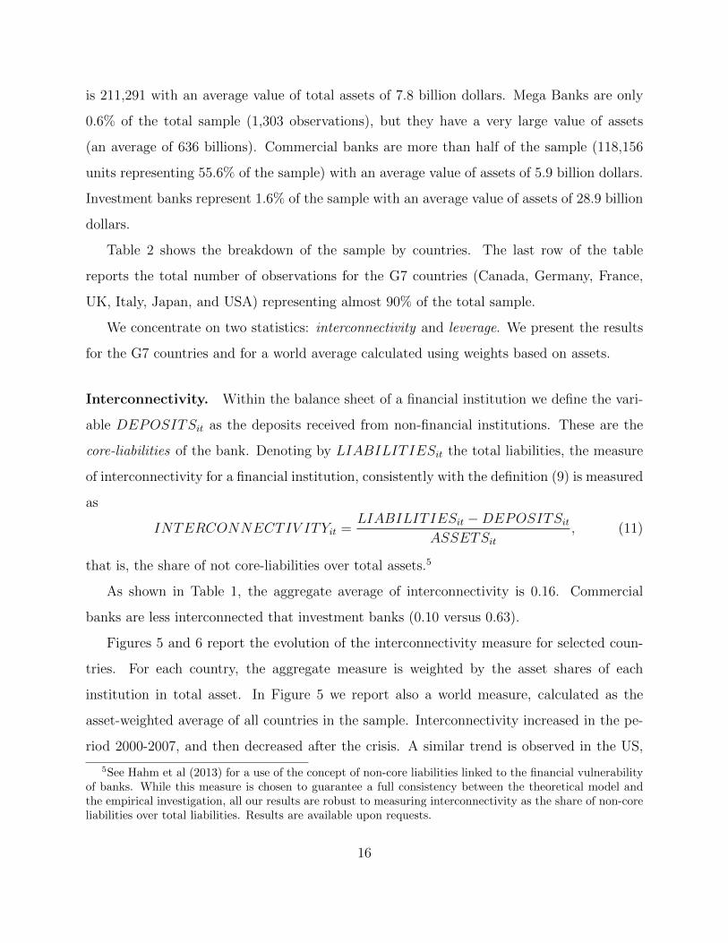
Interconnectivity. Within the balance sheet of a financial institution we define the vari-
able DEPOSITSit as the deposits received from non-financial institutions. These are the
core-liabilities of the bank. Denoting by LIABILITIESit the total liabilities, the measure
of interconnectivity for a financial institution, consistently with the definition (9) is measured
as
INTERCONNECTIV ITYit =LIABILITIESit −DEPOSITSit
ASSETSit, (11)
that is, the share of not core-liabilities over total assets.5
As shown in Table 1, the aggregate average of interconnectivity is 0.16. Commercial
banks are less interconnected that investment banks (0.10 versus 0.63).
Figures 5 and 6 report the evolution of the interconnectivity measure for selected coun-
tries. For each country, the aggregate measure is weighted by the asset shares of each
institution in total asset. In Figure 5 we report also a world measure, calculated as the
asset-weighted average of all countries in the sample. Interconnectivity increased in the pe-
riod 2000-2007, and then decreased after the crisis. A similar trend is observed in the US,
5See Hahm et al (2013) for a use of the concept of non-core liabilities linked to the financial vulnerabilityof banks. While this measure is chosen to guarantee a full consistency between the theoretical model andthe empirical investigation, all our results are robust to measuring interconnectivity as the share of non-coreliabilities over total liabilities. Results are available upon requests.
16
the UK, France and Germany. In Japan, Canada and Italy, instead, bank interconnectivity
does not show a clear trend.
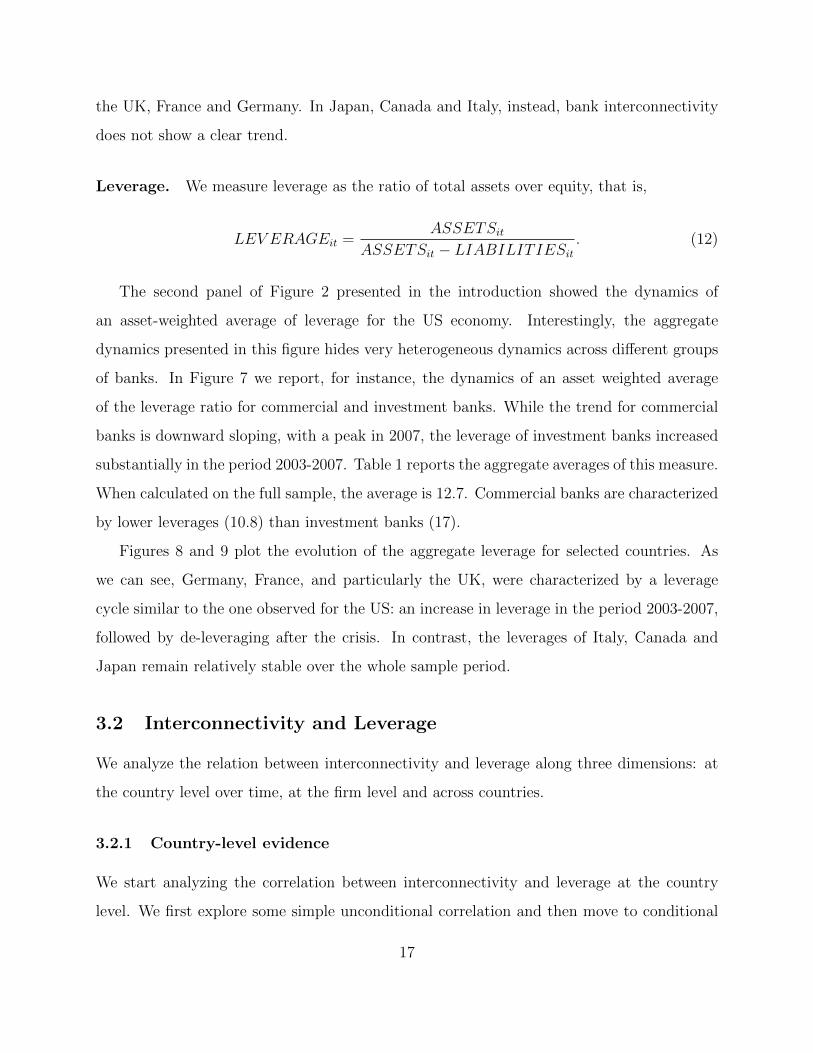
Leverage. We measure leverage as the ratio of total assets over equity, that is,
LEV ERAGEit =ASSETSit
ASSETSit − LIABILITIESit. (12)
The second panel of Figure 2 presented in the introduction showed the dynamics of
an asset-weighted average of leverage for the US economy. Interestingly, the aggregate
dynamics presented in this figure hides very heterogeneous dynamics across different groups
of banks. In Figure 7 we report, for instance, the dynamics of an asset weighted average
of the leverage ratio for commercial and investment banks. While the trend for commercial
banks is downward sloping, with a peak in 2007, the leverage of investment banks increased
substantially in the period 2003-2007. Table 1 reports the aggregate averages of this measure.
When calculated on the full sample, the average is 12.7. Commercial banks are characterized
by lower leverages (10.8) than investment banks (17).
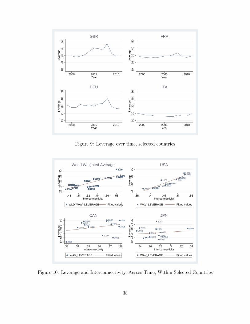
Figures 8 and 9 plot the evolution of the aggregate leverage for selected countries. As
we can see, Germany, France, and particularly the UK, were characterized by a leverage
cycle similar to the one observed for the US: an increase in leverage in the period 2003-2007,
followed by de-leveraging after the crisis. In contrast, the leverages of Italy, Canada and
Japan remain relatively stable over the whole sample period.
3.2 Interconnectivity and Leverage
We analyze the relation between interconnectivity and leverage along three dimensions: at
the country level over time, at the firm level and across countries.
3.2.1 Country-level evidence
We start analyzing the correlation between interconnectivity and leverage at the country
level. We first explore some simple unconditional correlation and then move to conditional
17

correlations.
Unconditional correlations. Figures 10 and 11 show scatter plots of the aggregate lever-
age ratio against our measure of interconnectivity within countries across time. France,
Germany and especially the UK present a strong positive correlation between leverage and
interconnectivity. In the UK, as for the US, we see a contemporaneous rise in intercon-
nectedness and leverage in the period 2003-2008 followed by a subsequent decline for both
variables. The similarity in the dynamics of interconnectedness and leverage for the US and
the UK might reflect the similarity of the financial sector in those two countries. On the other
hand, in Japan, Canada and Italy there is not a clear relation between interconnectivity and
leverage over time.
Figure 12 reports scatter plots for the leverage ratio and the interconnectedness measure
for all sample countries and for different years. Also in this case we observe a positive corre-
lation, which seems particularly strong in 2007 at the peak of the boom. On the one hand,
we have low-interconnected and low-leveraged financial systems in countries like Poland,
Turkey, and Mexico. On the other, we find highly interconnected and highly leveraged
financial systems in countries like Switzerland, UK and France.
Conditional correlations. We move to explore some conditional correlations at the ag-
gregate level with a simple two way fixed effect estimators. The results are reported in Table
3. In the first column we use interconnectivity as the only regressor. Thus, the coefficient
estimate represents the average slope for all years in the scatter plots presented in Figure 12.
Interestingly, variations in interconnectedness alone explain 38 percent of the variance in the
aggregate leverage. In the second and third columns, we add country and time fixed effects.
Apart from the fit of the regressions which increases substantially, the interconnectedness
coefficient remains positive and highly statistically significant.
While this subsection provides strong evidence of the existence of a positive correlation
between financial interconnectedness and leverage at the country level, the richness of micro
data available allows us to go a step further and investigate the existence of such a correlation
18
also at the micro level, that is, across banks.
3.2.2 Firm-level Evidence across all countries
We provide first some evidence for large banks, and then we move to the full sample.
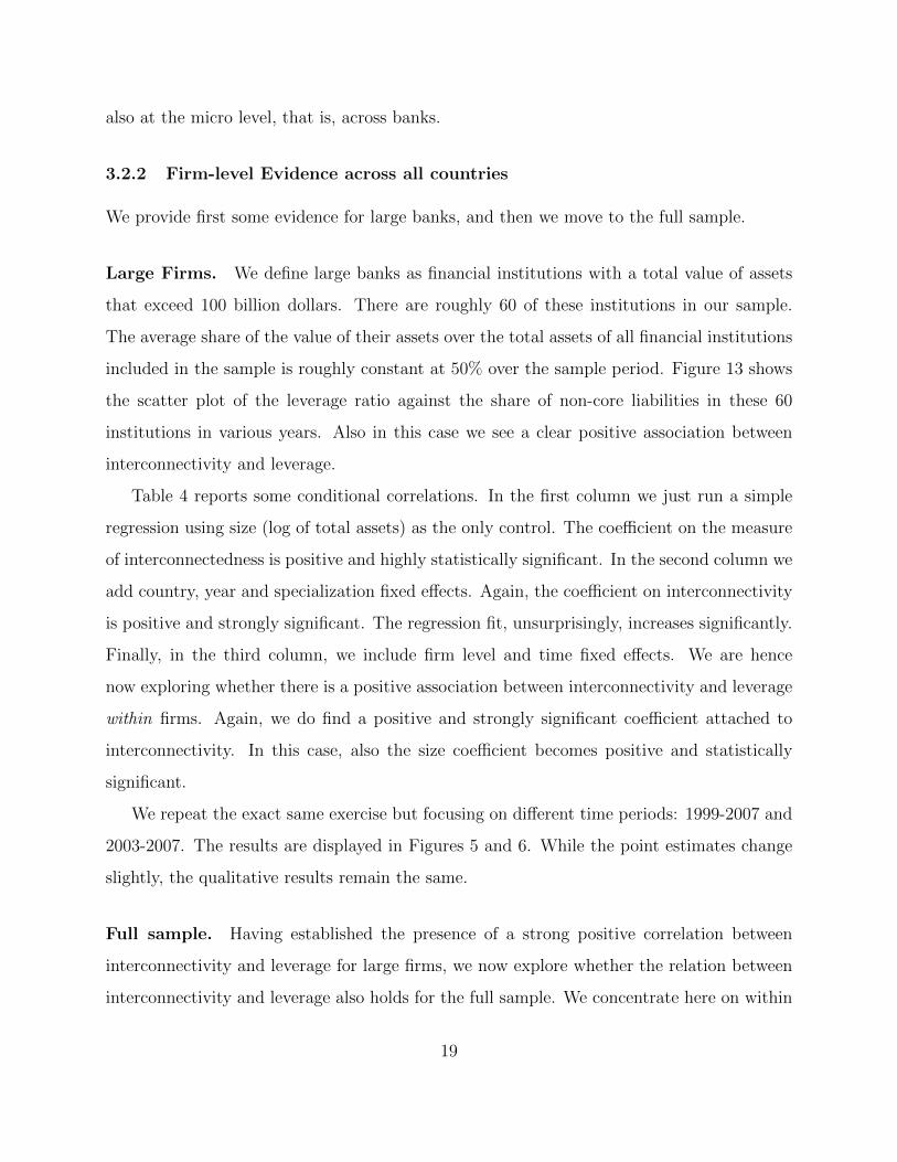
Large Firms. We define large banks as financial institutions with a total value of assets
that exceed 100 billion dollars. There are roughly 60 of these institutions in our sample.
The average share of the value of their assets over the total assets of all financial institutions
included in the sample is roughly constant at 50% over the sample period. Figure 13 shows
the scatter plot of the leverage ratio against the share of non-core liabilities in these 60
institutions in various years. Also in this case we see a clear positive association between
interconnectivity and leverage.
Table 4 reports some conditional correlations. In the first column we just run a simple
regression using size (log of total assets) as the only control. The coefficient on the measure
of interconnectedness is positive and highly statistically significant. In the second column we
add country, year and specialization fixed effects. Again, the coefficient on interconnectivity
is positive and strongly significant. The regression fit, unsurprisingly, increases significantly.
Finally, in the third column, we include firm level and time fixed effects. We are hence
now exploring whether there is a positive association between interconnectivity and leverage
within firms. Again, we do find a positive and strongly significant coefficient attached to
interconnectivity. In this case, also the size coefficient becomes positive and statistically
significant.
We repeat the exact same exercise but focusing on different time periods: 1999-2007 and
2003-2007. The results are displayed in Figures 5 and 6. While the point estimates change
slightly, the qualitative results remain the same.
Full sample. Having established the presence of a strong positive correlation between
interconnectivity and leverage for large firms, we now explore whether the relation between
interconnectivity and leverage also holds for the full sample. We concentrate here on within
19

firms relation, thus considering a two-way fixed effects estimator.
Table 7 contains the results. The three columns correspond to the three different time
periods used earlier. Again, we also condition on size which has a positive and highly
significant effect. As for the measure of interconnectivity, we continue to find a positive and
strongly significant coefficient. Therefore, we find a positive relation between leverage and
interconnectivity even if we do not restrict the sample to contain only the very large financial
institutions.
3.2.3 Firm-level evidence in selected countries
Finally, we explore whether the within firms results change across countries. In Table 8
we report the results obtained using a two-way fixed effects estimator in each of the G-7
countries, to explore the correlation between interconnectivity and leverage (conditioning on
the size of banks). We find positive and statistically significant coefficients for all of the G-7
countries with the only exception of Canada.
We conclude that, consistently with the model presented in Section 2, we find empirical
evidence of a strong association between interconnectivity and leverage: across firms, across
countries and across time.
3.3 Interconnectivity and return differential
The model presented in Section 2 implies the existence of a relation between interconnectivity
and the return differential on the assets and liabilities of banks. In this section we investigate
this relation empirically.
We define the empirical return differential as the difference between (i) the interest income
over the value of assets that earn interests, and (ii) the interest expenditures over the average
liabilities. Specifically,
DIFFERENTIALit =INT INCOMEitAV ASSETSit
− INT EXPitAV LIABILITIESit
.
20

While this measure does not reflect exactly the return differential as defined in the
model—see equation (10)—it is our closest empirical counterpart.
Figure 14 reports the world asset-weighted average of the return differential. Interestingly,
the figure shows a sharp decline in the boom phase of 2003-2007 and a mild increase since
then. In the next subsections we investigate the relation between the return differential and
interconnectivity at the country and firm level.
3.3.1 Country-level evidence
Figures 15 and 16 report the scatter plots of our measure of interconnectivity against the
return differential for some selected countries and for the world average. In most of the cases,
we can observe a strong negative relation between the two measures. The only notable
exception is France where the relation appears to be weakly positive. A strong negative
relation between interconnectivity and return differentials is also observed across countries
as shown in Figure 17.
Next we regress the measure of interconnectivity against the return differential condi-
tioning on country and time fixed effects. The results are shown in Table 9. Albeit the
consideration of time and country fixed effects reduces the magnitude of the coefficient,
we still find a negative and strongly statistically significant relation between interest rate
differential and interconnectivity.
3.3.2 Firm-level Evidence
Moving to the firm-level evidence, Figure 18 shows the scatter plot of interconnectivity
against the return differential for the sample of large banks in selected years. Again, we
find a strong negative association between these two variables, irrespective of the year under
consideration.
Tables 10 and 11 confirm the visual evidence through a regression analysis. The nega-
tive relation between interconnectivity and return differentials remains highly statistically
significant after controlling for firm size, specialization, time and country fixed effects. By
21

adding firm fixed effects we also find that the relation is negative within firms.
The finding that there is a negative relation between interconnectivity and return differ-
entials suggests that the choices of interconnectivity and leverage are mostly driven by the
diversification cost: banks choose to become more interconnected when it becomes easier to
diversify. This also suggests that the upward trends in interconnectivity and leverage ob-
served prior to the 2008-2009 crisis is more likely to have been driven by financial innovations
that made diversification easier for banks. This pattern, however, seems to have reverted
back after the crisis.
4 Conclusion
In this paper we have shown that there is a strong positive correlation between financial
interconnectivity and leverage across countries, over time, and across financial institutions.
The empirical evidence supports the theoretical results obtained in the first part of the paper.
The theoretical results are derived from a model in which banks choose, simultaneously,
the optimal diversification and the optimal leverage. Although cross-bank diversification
(interconnectivity) reduces the idiosyncratic risk for each bank, it does not eliminate the
aggregate or ‘systemic’ risk which is likely to increase when the leverage of the whole financial
sector increases. Our model provides a micro structure that can be embedded in a general
equilibrium framework to study the issue of interconnectivity and macroeconomic stability.
We leave the study of this issue for future research.
22

A Proof of Lemma 2.3
The bank problem is a standard intertemporal portfolio choice between a safe and riskyasset similar to the problem studied in Merton (1971). The solution takes the simple formthanks to the log-specification of the utility function together with constant return to scaleinvestments.
We now show that φt is strictly increasing in the adjusted return spread. From Lemma2.2 we know that the adjusted return differential Rk
t /Rlt is strictly increasing in Rk
t /Rlt.
Therefore, we only need to prove that φt is strictly increasing in the adjusted differentialRkt /R
lt. This can be proved by using the condition that determines φt from Lemma 2.3. For
convenience we rewrite this condition here
Et{
1
1 + [zt+1xt − 1]φt
}= 1, (13)
where we have used the variable xt = Rkt /R
lt to denote the adjusted return differential.
Using the implicit function theorem we derive
∂φt∂xt
= −Et{
zt+1φt[1+φt[zt+1xt−1]]2
}Et{
zt+1xt−1[1+φt[zt+1xt−1]]2
}Since the numerator is positive, the sign of the derivative depends on the denominator
which can be rewritten as
Et{
zt+1xt − 1
[1 + φt[zt+1xt − 1]]2
}= Et
{zt+1xt − 1
1 + φt[zt+1xt − 1]
}{1
1 + φt[zt+1xt − 1]
}= Et
{zt+1xt − 1
1 + φt[zt+1xt − 1]
}Et{
1
1 + φt[zt+1xt − 1]
}+
COV
{zt+1xt − 1
1 + φt[zt+1xt − 1],
1
1 + φt[zt+1xt − 1]
}The first expectation term on the right-hand side Et
{[zt+1xt−1]φt
1+[zt+1xt−1]φt
}can be rewritten as
Et{
11+[zt+1xt−1]φt
}− 1. By condition (13) this term is equal to zero. Therefore, we have
Et{
zt+1xt − 1
[1 + φt[zt+1xt − 1]]2
}= COV
{zt+1xt − 1
1 + φt[zt+1xt − 1],
1
1 + φt[zt+1xt − 1]
}The covariance is clearly negative because the first term is strictly increasing in zt+1 whilethe second term is strictly decreasing in zt+1. Therefore, ∂φt/∂xt > 0. �
23
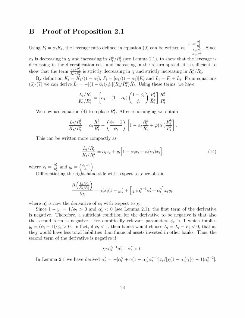
B Proof of Proposition 2.1
Using Ft = αtKt, the leverage ratio defined in equation (9) can be written as1+αt
Rkt
Rlt
1− Lt/Rlt
Kt/Rkt
. Since
αt is decreasing in χ and increasing in Rkt /R
lt (see Lemma 2.1), to show that the leverage is
decreasing in the diversification cost and increasing in the return spread, it is sufficient to
show that the termLt/Rl
t
Kt/Rkt
is strictly decreasing in χ and strictly increasing in Rkt /R
lt.
By definition Kt = Kt/(1− αt), Ft = [αt/(1− αt)]Kt and Lt = Ft + Lt. From equations(6)-(7) we can derive Lt = −[(1− φt)/φt](Rl
t/Rkt )Kt. Using these terms, we have
Lt/Rlt
Kt/Rkt
=
[αt − (1− αt)
(1− φtφt
)Rlt
Rkt
]Rkt
Rlt
.
We now use equation (4) to replace Rkt . After re-arranging we obtain
Lt/Rlt
Kt/Rkt
= αtRkt
Rlt
+
(φt − 1
φt
)[1− αt
Rkt
Rlt
+ ϕ(αt)Rkt
Rlt
].
This can be written more compactly as
Lt/Rlt
Kt/Rkt
= αtxt + yt
[1− αtxt + ϕ(αt)xt
], (14)
where xt =Rk
t
Rlt
and yt =(φt−1φt
).
Differentiating the right-hand-side with respect to χ we obtain
∂(Lt/Rl
t
Kt/Rkt
)∂χ
= α′txt(1− yt) +[χγαγ−1
t α′t + αγt
]xtyt,
where α′t is now the derivative of αt with respect to χ.Since 1 − yt = 1/φt > 0 and α′t < 0 (see Lemma 2.1), the first term of the derivative
is negative. Therefore, a sufficient condition for the derivative to be negative is that alsothe second term is negative. For empirically relevant parameters φt > 1 which impliesyt = (φt − 1)/φt > 0. In fact, if φt < 1, then banks would choose Lt = Lt − Ft < 0, that is,they would have less total liabilities than financial assets invested in other banks. Thus, thesecond term of the derivative is negative if
χγαγ−1t α′t + αγt < 0.
In Lemma 2.1 we have derived α′t = −[αγt + γ(1 − αt)αγ−1t ]xt/[χ(1 − αt)γ(γ − 1)αγ−2
t ].
24

Substituting in the above expression and re-arranging we obtain
1 <γxtγ − 1
+xtαt
(1− αt)(γ − 1).
Both terms on the right-hand-side are positive. Furthermore, since xt > 1 and γ > 1, thefirst term is bigger than 1. Therefore, the inequality is satisfied, proving that the derivativeof the leverage decreases in the diversification cost.
To show that the leverage ratio is decreasing in xt = Rkt /R
lt, we need to show that
Lt/Rlt
Kt/Rkt
is decreasing in xt. Differentiating the right-hand-side of (14) with respect to xt we obtain
∂(Lt/Rl
t
Kt/Rkt
)∂xt
= (1− yt)(α′txt + αt) + y′t
[1− αtxt + ϕ(αt)xt
]+ yt
[ϕ′t(αt)α
′txt + ϕ(αt)
],
where α′t is now the derivative of αt with respect to xt.Lemma 2.1 established that αt is increasing in xt = Rk
t /Rlt, that is, α′t > 0. Furthermore,
Lemma 2.3 established that φt is strictly increasing in xt = Rkt /R
lt, which implies that
yt =(φt−1φt
)is also increasing in xt = Rk
t /Rlt, that is, y′t > 0. Therefore, sufficient conditions
for the derivative to be positive are
φt > 1
1− αtxt + ϕ(αt)xt > 0 .
As argued above, the first condition (φt > 1) is satisfied for empirically relevant parameter-izations. For the second condition it is sufficient that αtxt ≤ 1, which is also satisfied forempirically relevant parameterizations. In fact, since in the data xt is not very different from1 (for example it is not bigger than 1.1), the condition allows αt to be close to 1 (about 90percent if xt is 1.1). Since αt represents the relative size of the interbank market comparedto the size of the whole banking sector, αt is significantly smaller than 1 in the data. There-fore, for empirically relevant parameterizations, leverage increases with the return spreadxt = Rk
t /Rlt.
The next step is to prove that the interconnectivity index is decreasing in χ and increasingin xt = Rk
t /Rlt. The index can be simplified to
αtxt1 + αtxt
.
Differentiating with respect to χ we obtain
∂INTERCONNECTIV ITY
∂χ=
α′txt(1 + αtxt)2
,
where α′t is the derivative of αt with respect to χ. As shown in Lemma 2.1, this is negative.Therefore, bank connectivity decreases in the diversification cost.
25

We now compute the derivative of interconnectivity with respect to xt and obtain
∂INTERCONNECTIV ITY
∂xt=
α′txt + αt(1 + αtxt)2
,
where α′t is the derivative of αt with respect to xt. As shown in Lemma 2.1, this is positive.Therefore, bank connectivity increases in the return spread. �
C Proof of Proposition 2.2
Taking into account that in aggregate Ft = αtKt, the bank differential return defined inequation (10) can be rewritten as
DIFFERENTIAL =
(xt − 1
1 + αtxt
)Rlt.
For notational simplicity we have used the variable xt = Rkt /R
lt.
Differentiating with respect to χ we obtain
∂DIFFERENTIAL
∂χ= −α
′txt(xt − 1)
(1 + αtxt)2Rlt,
where α′t is the derivative of αt with respect to χ. We have shown in Lemma 2.1 that thisderivative is negative. Therefore, the return differential increases in the differentiation cost.
Consider now the dependence of the bank return differential from the return spread. Thederivative of the return differential with respect to xt = Rk
t /Rlt is
∂DIFFERENTIAL
∂xt=
1 + αt + xt(1− xt)α′t(1 + αtxt)2
Rlt,
where α′t is the derivative of αt with respect to return spread xt. For the derivative to bepositive we need that the following condition is satisfied
1 + αt + xt(1− xt)α′t > 0.
In Lemma 2.1 we have derived α′t = 1/[(1 − αt)ϕ′′(αt)x
2t ]. Substituting in the above
expression and re-arranging we obtain
1− (1− α2t )ϕ
′′(αt) >1
xt.
We now use equation (2) to eliminate 1/xt and rewrite the condition as
ϕ(αt) + ϕ′(αt)− αtϕ′(αt) > (1− α2t )ϕ
′′(αt).
26

Using the functional form for the diversification cost specified in Assumption 1, the conditioncan be rewritten as (
1
γ − 1
)α +
[1 + γ2 − 2γ
γ(γ − 1)
]α2 > 1,
which is satisfied if αt is sufficiently small. Since αt is decreasing in χ, a sufficiently highvalue of χ guarantees that the bank return differential is increasing in the return spreadxt = Rk
t /Rlt. For example, when the diversification cost takes the quadratic form (γ = 2), it
is sufficient that αt ≤ 0.73. This upper bound for αt is significantly larger than the averagevalue observed for the whole banking sector. (See Figure 2 for the US). �
D Data Appendix
The data on bank balance sheets are taken from Bankscope, which is a comprehensive andglobal database containing information on 28,000 banks worldwide provided by Bureau vanDjik. Each bank report contains detailed consolidated and/or unconsolidated balance sheetand income statement. Since the data are expressed in national currency, we converted thenational figures in US dollars using the exchange rates provided by Bankscope.
An issue in the use of Bankscope data is the possibility of double counting of financialinstitutions. In fact, for a given Bureau van Djik id number (BVDIDNUM), which identi-fies uniquely a bank, in each given YEAR, it is possible to have several observations withvarious consolidation codes. There are eight different consolidation status in Bankscope:C1 (statement of a mother bank integrating the statements of its controlled subsidiaries orbranches with no unconsolidated companion), C2 (statement of a mother bank integratingthe statements of its controlled subsidiaries or branches with an unconsolidated companion),C* (additional consolidated statement), U1 (statement not integrating the statements ofthe possible controlled subsidiaries or branches of the concerned bank with no consolidatedcompanion), U2 (statement not integrating the statements of the possible controlled sub-sidiaries or branches of the concerned bank with a consolidated companion), U* (additionalunconsolidated statement) and A1 (aggregate statement with no companion).6 We polishedthe data in order to avoid duplicate observations and to favor consolidated statements overunconsolidated ones.
6See Bankscope user guide and Duprey and Le (2013) for additional details.
27

References
[1] Acemoglu, D., Ozdaglar, A. and A. Tahbaz-Salehi, 2015. “Systemic Risk and Stabilityin Financial Networks,” American Economic Review, 105(2): 564608
[2] Adrian, T. and H.S. Shin, 2010. “Liquidity and Leverage”, Journal of Financial Inter-mediation, Vol. 19(3): 418-437.
[3] Adrian, T. and H.S. Shin, 2011. “Financial Intermediary Balance Sheet Management,”Annual Review of Financial Economics, 3, 289-307.
[4] Adrian, T. and H.S. Shin, 2014. “Pro-cyclical Leverage and Value at Risk,” Review ofFinancial Studies, Vol. 27 (2), 373-403.
[5] Allahrakha, M., P. Glasserman, and H.P. Young, 2015. “Systemic Importance Indicatorsfor 33 U.S. Bank Holding Companies: An Overview of Recent Data”, Office of FinancialResearch, Brief Series.
[6] Allen, F. and D. Gale, 2000. “Financial Contagion,” Journal of Political Economy, Vol.108(1): 1-33.
[7] Billio, M., Getmansky, M., Lo, A.W. alnd L. Pelizzon, 2012. “Econometric measures ofconnectedness and systemic risk in the finance and insurance sectors,” Journal of FinancialEconomics, vol. 104(3): 535-559.
[8] Barattieri, A. Eden, M and Stevanovic, D. 2014. “Financial Interconnectedness and Mon-etary Policy Transmission”, mimeo.
[9] Cai, J., Saunders, A. and Steffen, S. 2014. “Syndication, Interconnectedness, and Sys-temic Risk”. mimeo.
[10] Cetorelli, N. and L. Goldberg, 2012 “Banking Globalization and Monetary Transmis-sion,” Journal of Finance, vol. 67(5): 1811-1843.
[11] David, A., and Lehar, A. 2011. “Why are Banks Highly Interconnected?”, mimeo.
[12] Devereux, M. and Yetman, J., 2010. “Leverage Constraints and the International Trans-mission of Shocks,” Journal of Monet, Credit and Banking, vol. 42: 71-105.
[13] Eisert, T. and Eufinger, C. 2014. “Interbank Network and Bank Bailouts: InsuranceMechanism for Non-Insured Creditors?”. SAFE Working Paper No. 10.
[14] Drehmann, M. and Tarashev, N. 2013. “Measuring the systemic importance of inter-connected banks”. Journal of Financial Intermediation. 22(4): 586-607.
[15] Freixas, X., Parigi, B.M. and J.C. Rochet, 2000. “Systemic Risk, Interbank Relations,and Liquidity Provision by the Central Bank ,”Journal of Money, Credit and Banking.Vol. 32(3): 611-638.
28

[16] Geanakoplos, J. 2010. “The Leverage Cycle,” In D. Acemoglu, K. Rogoff and M. Wood-ford, eds., NBER Macroeconomic Annual 2009, vol. 24: 1-65.
[17] Gennaioli, N., Schleifer, A. and R. W. Vishny, 2013. “A Model of Shadow Banking”The Journal of Finance Vol.68(4): 1331-1363.
[18] Hale, G., T. Kapan, and C. Minoiu, 2014. “Crisis Transmission in the Global BankingNetwork”, mimeo.
[19] Hahm, J.H., Shin, H.S. and Shin, K. 2013. “Non-Core Bank Liabilities and FinancialVulnerability,” Journal of Money, Credit and Banking Vol. 45(S1): 3-36.
[20] Liu, Z., S. Quiet, and B. Roth, 2015. “Banking sector interconnectedness: what is it,how can we measure it and why does it matter?”, Bank of England Quarterly Bulletin,2015 Q2.
[21] Merton, R.C., 1971. “Optimum Consumption and Portfolio Rules in a Continuous-TimeModel,” Journal of Economic Theory vol. 3(4): 373413.
[22] Nuno, G. and C. Thomas, 2012 “Bank Leverage Cycles”, Banco de Espana WorkingPaper No. 1222.
[23] Peltonen, T. A. Rancal, M. and P. Sarlin, 2015. “Interconnectedness of the bankingsector as a vulnerability to crises,” mimeo
[24] Shin, H. S. 2008.“Risk and Liquidity in a System Context,” Journal of Financial Inter-mediation Vol. 17 (3): 31529.
[25] Shin, H. S. 2009. “Securitisation and Financial Stability,” Economic Journal Vol. 119(536): 30932.
[26] Simsek, A. 2013.“Belief Disagreements and Collateral Constraints,” Econometrica, Vol.81(1): 1-53.
29
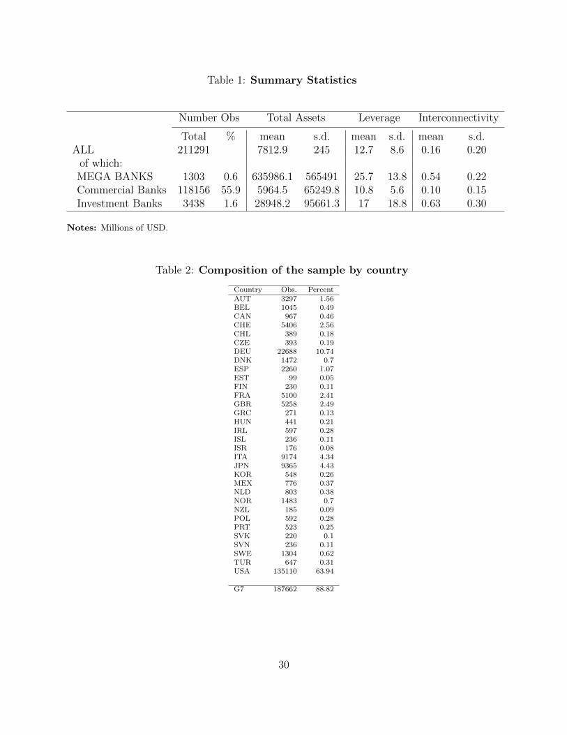
Table 1: Summary Statistics
Number Obs Total Assets Leverage Interconnectivity
Total % mean s.d. mean s.d. mean s.d.ALL 211291 7812.9 245 12.7 8.6 0.16 0.20
of which:MEGA BANKS 1303 0.6 635986.1 565491 25.7 13.8 0.54 0.22Commercial Banks 118156 55.9 5964.5 65249.8 10.8 5.6 0.10 0.15Investment Banks 3438 1.6 28948.2 95661.3 17 18.8 0.63 0.30
Notes: Millions of USD.
Table 2: Composition of the sample by country
Country Obs. PercentAUT 3297 1.56BEL 1045 0.49CAN 967 0.46CHE 5406 2.56CHL 389 0.18CZE 393 0.19DEU 22688 10.74DNK 1472 0.7ESP 2260 1.07EST 99 0.05FIN 230 0.11FRA 5100 2.41GBR 5258 2.49GRC 271 0.13HUN 441 0.21IRL 597 0.28ISL 236 0.11ISR 176 0.08ITA 9174 4.34JPN 9365 4.43KOR 548 0.26MEX 776 0.37NLD 803 0.38NOR 1483 0.7NZL 185 0.09POL 592 0.28PRT 523 0.25SVK 220 0.1SVN 236 0.11SWE 1304 0.62TUR 647 0.31USA 135110 63.94
G7 187662 88.82
30
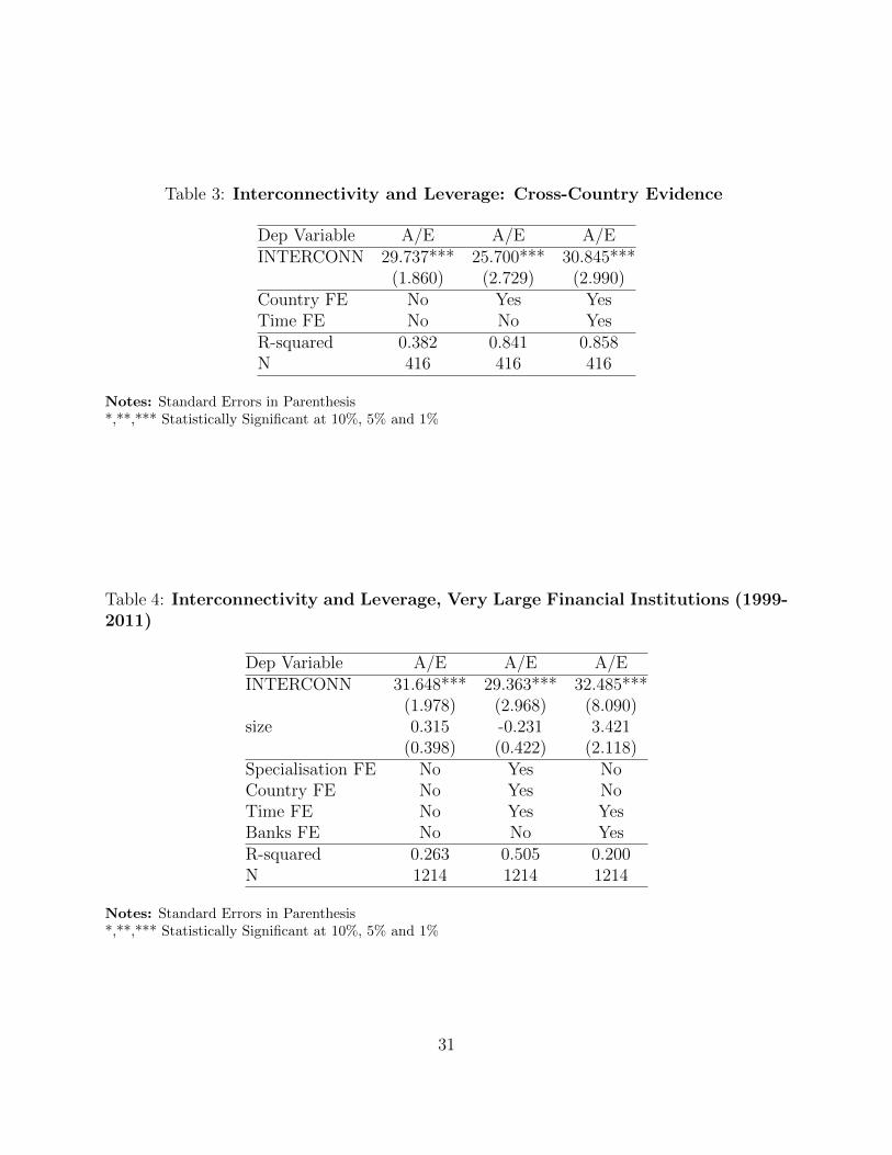
Table 3: Interconnectivity and Leverage: Cross-Country Evidence
Dep Variable A/E A/E A/EINTERCONN 29.737*** 25.700*** 30.845***
(1.860) (2.729) (2.990)Country FE No Yes YesTime FE No No YesR-squared 0.382 0.841 0.858N 416 416 416
Notes: Standard Errors in Parenthesis*,**,*** Statistically Significant at 10%, 5% and 1%
Table 4: Interconnectivity and Leverage, Very Large Financial Institutions (1999-2011)
Dep Variable A/E A/E A/EINTERCONN 31.648*** 29.363*** 32.485***
(1.978) (2.968) (8.090)size 0.315 -0.231 3.421
(0.398) (0.422) (2.118)Specialisation FE No Yes NoCountry FE No Yes NoTime FE No Yes YesBanks FE No No YesR-squared 0.263 0.505 0.200N 1214 1214 1214
Notes: Standard Errors in Parenthesis*,**,*** Statistically Significant at 10%, 5% and 1%
31

Table 5: Interconnectivity and Leverage, Very Large Financial Institutions (1999-2007)
Dep Variable A/E A/E A/EINTERCONN 32.758*** 28.636*** 33.013***
(1.848) (2.409) (4.653)size 0.471 -0.617 3.514***
(0.543) (0.562) (1.198)Specialisation FE No Yes NoCountry FE No Yes NoTime FE No Yes YesBanks FE No No YesR-squared 0.278 0.525 0.173N 820 820 820
Notes: Standard Errors in Parenthesis*,**,*** Statistically Significant at 10%, 5% and 1%
Table 6: Interconnectivity and Leverage, Very Large Financial Institutions (2003-2007)
Dep Variable A/E A/E A/EINTERCONN 35.924*** 34.494*** 44.612***
(2.607) (3.392) (6.223)size 0.130 -0.337 8.441***
(0.772) (0.764) (1.804)Specialisation FE No Yes NoCountry FE No Yes NoTime FE No Yes YesBanks FE No No YesR-squared 0.284 0.544 0.277N 482 482 482
Notes: Standard Errors in Parenthesis*,**,*** Statistically Significant at 10%, 5% and 1%
32
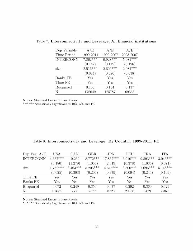
Table 7: Interconnectivity and Leverage, All financial institutions
Dep Variable A/E A/E A/ETime Period 1999-2011 1999-2007 2003-2007INTERCONN 7.862*** 6.928*** 5.082***
(0.142) (0.149) (0.196)size 2.516*** 2.606*** 2.981***
(0.024) (0.026) (0.038)Banks FE Yes Yes YesTime FE Yes Yes YesR-squared 0.106 0.134 0.137N 176649 125787 69563
Notes: Standard Errors in Parenthesis*,**,*** Statistically Significant at 10%, 5% and 1%
Table 8: Interconnectivity and Leverage: By Country, 1999-2011, FE
Dep Var: A/E USA CAN GBR JPN DEU FRA ITAINTERCONN 4.637*** -0.239 8.772*** 17.852*** 6.910*** 9.593*** 3.046***
(0.180) (1.279) (1.053) (2.019) (0.378) (1.035) (0.371)size 1.752*** 3.463*** 5.205*** 4.645*** 3.500*** 7.696*** 5.148***
(0.025) (0.303) (0.206) (0.379) (0.094) (0.244) (0.109)Time FE Yes Yes Yes Yes Yes Yes YesBanks FE Yes Yes Yes Yes Yes Yes YesR-squared 0.072 0.249 0.350 0.077 0.392 0.360 0.329N 113369 777 2577 8723 20956 3479 8367
Notes: Standard Errors in Parenthesis*,**,*** Statistically Significant at 10%, 5% and 1%
33

Table 9: Interconnectivity and Return Differential: Cross-Country Evidence
Dep Variable INTERCONN INTERCONN INTERCONNDifferential -0.069*** -0.042*** -0.029***
(0.004) (0.005) (0.005)Country FE No Yes YesTime FE No No YesR-squared 0.421 0.893 0.910N 416 416 416
Notes: Standard Errors in Parenthesis*,**,*** Statistically Significant at 10%, 5% and 1%
Table 10: Interconnectivity and Return Differential, Very Large Financial Insti-tutions (1999-2011)
Dep Variable INTERCONN INTERCONN INTERCONNDifferential -0.098*** -0.110*** -0.025*
(0.006) (0.008) (0.013)size -0.013* -0.003 0.076**
(0.007) (0.007) (0.031)Specialisation FE No Yes NoCountry FE No Yes NoTime FE No Yes YesBanks FE No No YesR-squared 0.226 0.680 0.229N 963 963 963
Notes: Standard Errors in Parenthesis*,**,*** Statistically Significant at 10%, 5% and 1%
34

Table 11: Interconnectivity and Return Differential, All Financial Institutions(1999-2011)
Dep Variable INTERCONN INTERCONN INTERCONNDifferential -0.039*** -0.019*** -0.006***
(0.001) (0.000) (0.001)size 0.043*** 0.034*** 0.038***
(0.000) (0.000) (0.002)Specialisation FE No Yes NoCountry FE No Yes NoTime FE No Yes YesBanks FE No No YesR-squared 0.365 0.576 0.071N 169372 169372 169362
Notes: Standard Errors in Parenthesis*,**,*** Statistically Significant at 10%, 5% and 1%
35

.2.3
.4.5
.6In
terc
onne
ctiv
ity
2000 2005 2010Year
World Weighted Average
.2.3
.4.5
.6In
terc
onne
ctiv
ity
2000 2005 2010Year
USA
.2.3
.4.5
.6In
terc
onne
ctiv
ity
2000 2005 2010Year
CAN
.2.3
.4.5
.6In
terc
onne
ctiv
ity
2000 2005 2010Year
JPN
Figure 5: Interconnectivity over time, selected countries.
.5.5
5.6
.65
.7.7
5In
terc
onne
ctiv
ity
2000 2005 2010Year
GBR
.5.5
5.6
.65
.7.7
5In
terc
onne
ctiv
ity
2000 2005 2010Year
FRA
.5.5
5.6
.65
.7.7
5In
terc
onne
ctiv
ity
2000 2005 2010Year
DEU
.5.5
5.6
.65
.7.7
5In
terc
onne
ctiv
ity
2000 2005 2010Year
ITA
Figure 6: Interconnectivity over time, selected countries.
36

1011
1213
Leve
rage
2000 2005 2010Year
Commercial Banks
3035
4045
50Le
vera
ge
2000 2005 2010Year
Investment Banks
Figure 7: Leverage over time, USA, Commercial and Investment Banks
1520
2530
Leve
rage
2000 2005 2010Year
World Weighted Average
1520
2530
Leve
rage
2000 2005 2010Year
USA
1520
2530
Leve
rage
2000 2005 2010Year
CAN
1520
2530
Leve
rage
2000 2005 2010Year
JPN
Figure 8: Leverage over time, selected countries
37
1020
3040
50Le
vera
ge
2000 2005 2010Year
GBR
1020
3040
50Le
vera
ge
2000 2005 2010Year
FRA
1020
3040
50Le
vera
ge
2000 2005 2010Year
DEU
1020
3040
50Le
vera
ge
2000 2005 2010Year
ITA
Figure 9: Leverage over time, selected countries
1999
200020012002
20032004 2005
20062007
2008
20092010
20111999
200020012002
20032004 2005
20062007
2008
20092010
20111999
200020012002
20032004 2005
20062007
2008
20092010
20111999
200020012002
20032004 2005
20062007
2008
20092010
20111999
200020012002
20032004 2005
20062007
2008
20092010
20111999
200020012002
20032004 2005
20062007
2008
20092010
20111999
200020012002
20032004 2005
20062007
2008
20092010
20111999
200020012002
20032004 2005
20062007
2008
20092010
20111999
200020012002
20032004 2005
20062007
2008
20092010
20111999
200020012002
20032004 2005
20062007
2008
20092010
20111999
200020012002
20032004 2005
20062007
2008
20092010
20111999
200020012002
20032004 2005
20062007
2008
20092010
20111999
200020012002
20032004 2005
20062007
2008
20092010
20111999
200020012002
20032004 2005
20062007
2008
20092010
20111999
200020012002
20032004 2005
20062007
2008
20092010
20111999
200020012002
20032004 2005
20062007
2008
20092010
20111999
200020012002
20032004 2005
20062007
2008
20092010
20111999
200020012002
20032004 2005
20062007
2008
20092010
20111999
200020012002
20032004 2005
20062007
2008
20092010
20111999
200020012002
20032004 2005
20062007
2008
20092010
20111999
200020012002
20032004 2005
20062007
2008
20092010
20111999
200020012002
20032004 2005
20062007
2008
20092010
20111999
200020012002
20032004 2005
20062007
2008
20092010
20111999
200020012002
20032004 2005
20062007
2008
20092010
20111999
200020012002
20032004 2005
20062007
2008
20092010
20111999
200020012002
20032004 2005
20062007
2008
20092010
20111999
200020012002
20032004 2005
20062007
2008
20092010
20111999
200020012002
20032004 2005
20062007
2008
20092010
20111999
200020012002
20032004 2005
20062007
2008
20092010
20111999
200020012002
20032004 2005
20062007
2008
20092010
20111999
200020012002
20032004 2005
20062007
2008
20092010
20111999
200020012002
20032004 2005
20062007
2008
20092010
2011
2224
2628
30Le
vera
ge
.48 .5 .52 .54 .56 .58Interconnectivity
WLD_WAV_LEVERAGE Fitted values
World Weighted Average
1999 200020012002
200320042005
20062007
2008
200920102011
1520
2530
Leve
rage
.35 .4 .45 .5 .55Interconnectivity
WAV_LEVERAGE Fitted values
USA
19992000
20012002
2003
20042005
2006
20072008
2009
20102011
1718
1920
2122
Leve
rage
.33 .34 .35 .36 .37 .38Interconnectivity
WAV_LEVERAGE Fitted values
CAN
1999
2000 2001
2002
2003
20042005
20062007
2008
2009
20102011
2022
2426
2830
Leve
rage
.24 .26 .28 .3 .32 .34Interconnectivity
WAV_LEVERAGE Fitted values
JPN
Figure 10: Leverage and Interconnectivity, Across Time, Within Selected Countries
38

1999200020012002
2003
2004
200520062007
2008
2009
2010201125
3035
4045
Leve
rage
.55 .6 .65 .7 .75Interconnectivity
WAV_LEVERAGE Fitted values
GBR
1999
2000200120022003
2004
20052006
2007
2008
20092010
2011
2628
3032
34Le
vera
ge
.62 .64 .66 .68 .7 .72Interconnectivity
WAV_LEVERAGE Fitted values
FRA
1999
20002001
20022003
2004
2005
20062007
2008
2009
20102011
2530
3540
Leve
rage
.5 .52 .54 .56 .58 .6Interconnectivity
WAV_LEVERAGE Fitted values
DEU1999
2000
20012002
20032004 200520062007
2008
20092010
2011
1617
1819
20Le
vera
ge
.51 .52 .53 .54Interconnectivity
WAV_LEVERAGE Fitted values
ITA
Figure 11: Leverage and Interconnectivity, Across Time, Within Selected Countries
AUT
BEL
CAN
CHE
CHLCZE
DEU
DNK
ESP
EST
FIN
FRAGBR
GRCHUN
IRL
ISL
ISRITA
JPNKOR
MEX
NLD
NOR
NZL
POL
PRT
SVKSVN
SWE
TUR
USA
1015
2025
3035
0 .2 .4 .6 .8INTERCONN
WAV_LEVERAGE Fitted values
2001
AUT
BEL
CAN
CHE
CHLCZE
DEU
DNK
ESP
ESTFIN
FRA
GBR
GRC
HUN
IRL
ISL
ISRITA
JPN
KOR
MEX
NLD
NOR
NZL
POL
PRT
SVK SVN
SWE
TUR
USA
1015
2025
3035
0 .2 .4 .6 .8INTERCONN
WAV_LEVERAGE Fitted values
2003
AUT
BEL
CAN
CHE
CHLCZE
DEU
DNK
ESPEST FIN
FRA
GBR
GRCHUN
IRL
ISLISR ITA
JPN
KOR
MEX
NLD
NORNZL
POL
PRTSVK SVN
SWE
TUR
USA
1020
3040
.2 .4 .6 .8INTERCONN
WAV_LEVERAGE Fitted values
2007
AUT
BEL
CAN
CHE
CHLCZE
DEU DNKESP
EST
FIN
FRAGBR
GRCHUN
IRL
ISL
ISR ITA
JPN
KORMEX
NLD
NORNZL
POL
PRTSVK
SVN
SWE
TUR
USA
010
2030
40
.2 .4 .6 .8INTERCONN
WAV_LEVERAGE Fitted values
2010
Figure 12: Leverage and Interconnectivity, Across countries, Selected Years
39

1020
3040
5060
.2 .4 .6 .8 1INTERCONN
= assets/ totalequity Fitted values
2001
1020
3040
5060
0 .2 .4 .6 .8 1INTERCONN
= assets/ totalequity Fitted values
2003
020
4060
.2 .4 .6 .8 1INTERCONN
= assets/ totalequity Fitted values
2007
020
4060
0 .2 .4 .6 .8 1INTERCONN
= assets/ totalequity Fitted values
2010
Figure 13: Leverage and Interconnectivity, Across Very Large Firms, Selected Years
1.2
1.4
1.6
1.8
2D
IFF
ER
EN
TIA
L
2000 2005 2010Year
World Weighed Average of Differential
Figure 14: Return Differential over Time
40

19992000
20012002
2003
2004
2005
20062007 2008
200920102011
19992000
20012002
2003
2004
2005
20062007 2008
200920102011
19992000
20012002
2003
2004
2005
20062007 2008
200920102011
19992000
20012002
2003
2004
2005
20062007 2008
200920102011
19992000
20012002
2003
2004
2005
20062007 2008
200920102011
19992000
20012002
2003
2004
2005
20062007 2008
200920102011
19992000
20012002
2003
2004
2005
20062007 2008
200920102011
19992000
20012002
2003
2004
2005
20062007 2008
200920102011
19992000
20012002
2003
2004
2005
20062007 2008
200920102011
19992000
20012002
2003
2004
2005
20062007 2008
200920102011
19992000
20012002
2003
2004
2005
20062007 2008
200920102011
19992000
20012002
2003
2004
2005
20062007 2008
200920102011
19992000
20012002
2003
2004
2005
20062007 2008
200920102011
19992000
20012002
2003
2004
2005
20062007 2008
200920102011
19992000
20012002
2003
2004
2005
20062007 2008
200920102011
19992000
20012002
2003
2004
2005
20062007 2008
200920102011
19992000
20012002
2003
2004
2005
20062007 2008
200920102011
19992000
20012002
2003
2004
2005
20062007 2008
200920102011
19992000
20012002
2003
2004
2005
20062007 2008
200920102011
19992000
20012002
2003
2004
2005
20062007 2008
200920102011
19992000
20012002
2003
2004
2005
20062007 2008
200920102011
19992000
20012002
2003
2004
2005
20062007 2008
200920102011
19992000
20012002
2003
2004
2005
20062007 2008
200920102011
19992000
20012002
2003
2004
2005
20062007 2008
200920102011
19992000
20012002
2003
2004
2005
20062007 2008
200920102011
19992000
20012002
2003
2004
2005
20062007 2008
200920102011
19992000
20012002
2003
2004
2005
20062007 2008
200920102011
19992000
20012002
2003
2004
2005
20062007 2008
200920102011
19992000
20012002
2003
2004
2005
20062007 2008
200920102011
19992000
20012002
2003
2004
2005
20062007 2008
200920102011
19992000
20012002
2003
2004
2005
20062007 2008
200920102011
19992000
20012002
2003
2004
2005
20062007 2008
200920102011
.45
.5.5
5In
terc
onne
ctiv
ity
1.2 1.4 1.6 1.8 2DIFFERENTIAL
WLD_WAV_NON_CORE_LIAB Fitted values
World Weighted Average
1999
200020012002
200320042005
20062007
2008
20092010
2011
.35
.4.4
5.5
.55
Inte
rcon
nect
ivity
2.6 2.8 3 3.2 3.4DIFFERENTIAL
WAV_NON_CORE_LIAB_share Fitted values
USA
1999
2000
2001
200220032004
2005
2006
2007
2008
2009
2010
2011
.33
.34
.35
.36
.37
.38
Inte
rcon
nect
ivity
1.4 1.6 1.8 2 2.2DIFFERENTIAL
WAV_NON_CORE_LIAB_share Fitted values
CAN
1999
2000
2001
2002
2003200420052006
2007
2008
2009
20102011
.24
.26
.28
.3.3
2.3
4In
terc
onne
ctiv
ity
.9 1 1.1 1.2 1.3DIFFERENTIAL
WAV_NON_CORE_LIAB_share Fitted values
JPN
Figure 15: Interconnectivity and Return Differential, Across Time, Within Selected Coun-tries
199920002001 2002
2003
2004
200520062007
2008
20092010
2011
.55
.6.6
5.7
.75
Inte
rcon
nect
ivity
.6 .8 1 1.2 1.4 1.6DIFFERENTIAL
WAV_NON_CORE_LIAB_share Fitted values
GBR
19992000
20012002 2003
2004
20052006
2007
2008
2009
20102011
.62
.64
.66
.68
.7.7
2In
terc
onne
ctiv
ity
0 .2 .4 .6 .8 1DIFFERENTIAL
WAV_NON_CORE_LIAB_share Fitted values
FRA
199920002001
2002200320042005
20062007
2008
20092010
2011
.5.5
2.5
4.5
6.5
8.6
Inte
rcon
nect
ivity
.6 .8 1 1.2 1.4DIFFERENTIAL
WAV_NON_CORE_LIAB_share Fitted values
DEU
1999
2000
2001
2002
20032004
2005
20062007
2008
20092010
2011
.51
.52
.53
.54
Inte
rcon
nect
ivity
1.6 1.8 2 2.2 2.4 2.6DIFFERENTIAL
WAV_NON_CORE_LIAB_share Fitted values
ITA
Figure 16: Interconnectivity and Return Differential, Across Time, Within Selected Coun-tries
41

AUT
BEL CAN
CHE
CHLCZE
DEU
DNK
ESP
EST
FIN
FRAGBR
GRC HUN
IRL
ISL
ISR
ITA
JPN
KOR
MEX
NLDNOR
NZL
POL
PRT
SVKSVN
SWE
TUR
USA
0.2
.4.6
.8In
terc
onne
ctiv
ity
0 2 4 6 8DIFFERENTIAL
WAV_NON_CORE_LIAB_share Fitted values
2001
AUTBEL
CAN
CHE
CHL
CZE
DEU
DNK
ESP
EST
FIN
FRAGBR
GRC HUN
IRLISL
ISR
ITA
JPNKOR
MEX
NLD NOR
NZL
POL
PRT
SVK
SVN
SWE
TUR
USA
0.2
.4.6
.8In
terc
onne
ctiv
ity
0 2 4 6DIFFERENTIAL
WAV_NON_CORE_LIAB_share Fitted values
2003
AUTBEL
CAN
CHE
CHLCZE
DEU
DNK
ESP EST
FIN
FRAGBR
GRCHUN
IRLISL
ISR
ITA
JPN
KOR
MEX
NLDNOR
NZL
POL
PRT
SVK
SVN
SWE
TUR
USA
0.2
.4.6
.8In
terc
onne
ctiv
ity
0 2 4 6 8DIFFERENTIAL
WAV_NON_CORE_LIAB_share Fitted values
2007
AUTBEL
CAN
CHE
CHL
CZE
DEU
DNK
ESP
EST
FIN FRAGBR
GRC HUN
IRL
ISL
ISR
ITA
JPN
KORMEX
NLDNORNZL
POL
PRT
SVK
SVN
SWE
TUR
USA
.2.4
.6.8
Inte
rcon
nect
ivity
1 2 3 4 5DIFFERENTIAL
WAV_NON_CORE_LIAB_share Fitted values
2010
Figure 17: Interconnectivity and Return Differential, Across Countries, Selected Years
.2.4
.6.8
1In
terc
onne
ctiv
ity
−2 0 2 4 6DIFFERENTIAL
NON_CORE_LIAB_share Fitted values
2001
0.2
.4.6
.81
Inte
rcon
nect
ivity
0 2 4 6 8DIFFERENTIAL
NON_CORE_LIAB_share Fitted values
2003
.2.4
.6.8
1In
terc
onne
ctiv
ity
−2 0 2 4 6DIFFERENTIAL
NON_CORE_LIAB_share Fitted values
2007
0.2
.4.6
.81
Inte
rcon
nect
ivity
−2 0 2 4 6DIFFERENTIAL
NON_CORE_LIAB_share Fitted values
2010
Figure 18: Interconnectivity and Return Differential, Across Very Large Firms, SelectedYears
42