Banks, Firms, and Jobs∗

Fabio Berton† Sauro Mocetti‡ Andrea F. Presbitero§ Matteo Richiardi¶

December 12, 2016

Abstract: Unemployment is one of the most visible effects of financial crises. We contributeto the empirical literature on the employment effects of a decline in bank credit, investigatingindividual heterogeneity across firms, workers and jobs in the response to a financial shock.We use a rich data set of over 1.5 million individual job contracts in an Italian region, thatis matched with the universe of firms and their lending banks. To isolate the effect of the fi-nancial shock we construct a firm-specific time-varying measure of credit supply. Our findingsindicate that a 10 percent supply-driven credit contraction reduces employment by 2.5 percent.The effect is mostly concentrated among the relatively less educated and less skilled workerswith temporary contracts, and is consistent with the presence of a “dual” labor market and askill upgrade strategy adopted by firms in response to the financial shock.

JEL Codes: G01; G21; J23; J63

Keywords: Bank lending channel; Job contracts; Employment; Financing constraints; Skillupgrade

∗The views expressed in this paper are those of the authors and do not necessarily represent those of the Bankof Italy, IMF, or IMF policy. We wish to thank Isha Agarwal, Tobias Berg (discussant), Mihai Copaciu (discussant),Romaine Duval, Francesco Manaresi (discussant), Camelia Minoiu, Michael Neugart, Roman Raluca (discussant),Enrico Sette, Nikola Spatafora, and participants to the 2nd IWH-FIN-FIRE workshop on “Challenges on FinancialStability”, Chicago Financial Institutions Conference (Chicago, 2016), 28th EALE Conference (Ghent, 2016), 33rd

International Symposium on Money, Banking and Finance (Clermont-Ferrand, 2016), the Annual Conference ofthe Italian Economic Association (Naples, 2015) and the Annual Conferences of the Italian Association of LabourEconomists (Cagliari, 2015; Trento, 2016), and at seminars at the Bank of Italy, Federal Reserve Board, InternationalMonetary Fund, and University of Torino for helpful comments and suggestions. Financial support from the Uni-versity of Torino and Compagnia di San Paolo Bank Foundation with project “Skill mismatch: measurement issuesand consequences for innovative and inclusive societies” is kindly acknowledged. The usual disclaimers apply.†University of Torino. E-mail: fabio.berton@unito.it.‡Bank of Italy. E-mail: sauro.mocetti@bancaditalia.it.§International Monetary Fund and MoFiR. E-mail: apresbitero@imf.org.¶Institute for New Economic Thinking, University of Oxford; Nuffield College, and Collegio Carlo Alberto.

E-mail: matteo.richiardi@maths.ox.ac.uk.

1 Introduction

In the aftermath of the global financial crisis, a severe credit crunch has had long lasting con-

sequences on a number of advanced economies, where unemployment rates have increased

markedly. These facts have triggered a renewed interest on the relationship between finance

and employment (Pagano and Pica, 2012) and, specifically, on the effects of credit supply

shocks have on firms’ employment decisions (Chodorow-Reich, 2014; Duygan-Bump et al.,

2015).

While this literature provides original insights on the effects of financial crises on total

employment at the firm or state level, it is generally silent about within-firm dynamics. For

instance, little is knows about the impact of a decline in firm financing on different types of

jobs. We contribute to this strand of literature by zooming in on the employment dynamics

within the firm and by providing a series of novel findings on how firms adjust the level and

composition of the labor force in response to credit shocks. We do so thanks to the availability

of an original and extremely rich data set, that draws on an administrative archive that collects

daily information on individual job contracts and labor market flows. The dataset covers the

universe of firms, including micro-enterprises, in an Italian region, matched with their lending

banks through the Italian Credit Register. We end up with a quarterly dataset of about 200,000

firms, spanning the period from 2008:Q1 to 2012:Q4 for which, thanks to the degree of gran-

ularity of the data, we can go beyond the standard job destruction/job creation dichotomy

to investigate differential responses to a credit supply shocks across firms, workers, and job

contracts.

We find that a 10 percent supply-driven credit contraction reduces employment by 2.5 per-

cent. This effect is concentrated among individuals employed with temporary contracts and

occurred mostly through more outflows rather than less inflows. This result is consistent with

the existence of a “dual” labor market. The reduction of employment was concentrated among

the relatively less educated individuals, who are employed in jobs with lower skill content. Im-

migrant and younger workers were also hit disproportionately more by the credit rationing,

reflecting the prevalence of immigrants in low-skill occupations, and the lower tenure and the

higher presence of younger workers in temporary jobs. The stronger impact on the less edu-

cated workers is consistent with the notion that during recessions firms adopt a skill upgrading

strategy (Hershbein and Kahn, 2016). This strategy is pursued mostly by allowing temporary

contracts to expire, and not renewing them, possibly because of the lower training and hiring

costs (and therefore also firms’ lower incentives for labor hoarding) for this segment of the

population. By contrast, less educated workers with open-ended contracts are unaffected by

3

firms’ financing constraints. Therefore, skill upgrading strategies are heavily shaped by con-

tracts regulation. To shed light on the mechanisms linking the financial crisis to employment

outcomes, we find that firms that are more reliant on bank credit, that use more intensively

granted credit, and that have weaker relationships with banks, experience a greater reduction

in the availability of bank financing.

This paper contributes to the growing literature on the real effect of credit supply shocks

(Amiti and Weinstein, 2011, 2016; Cingano et al., 2016; Paravisini et al., 2015) and is most closely

related to the recent contributions that investigate the effects of a reduction in credit supply

on employment outcomes at the firm level (Chodorow-Reich, 2014; Benmelech et al., 2015;

Bottero et al., 2015; Bentolila et al., 2015; Berg, 2016; Hochfellner et al., 2016; Popov and Rocholl,

2016; Siemer, 2016).1 Drawing on micro-level datasets, these studies consistently show that a

tightening of the credit supply leads to a contraction of the labor force.

The analysis by Bentolila et al. (2015) has the unique feature of being based on loan level

data from a credit register. Relying on the differences in bank health at the beginning of the

financial crisis, the paper shows that firms exposed to weak banks contracted employment by

2.2 percentage points more than firms that were borrowing from healthier lenders, and results

are able to explain about a fourth of the fall in aggregate employment in Spain between 2007

and 2010. Hochfellner et al. (2016) use employer-employee matched data for a sample of Ger-

man firms to look at how individual characteristics affect labor outcomes. The identification

strategy hinges on differences between firms that were affected or not by the credit shock, de-

pending on their location in the seven federal states where the major bank was one of the five

Landesbanks with significant exposure to the U.S. mortgage crisis. In addition to confirming the

aggregate negative effect of credit contraction on employment, Hochfellner et al. (2016) show

that workers in firms which have been exposed to a negative credit shock experience signifi-

cant earning losses and an increase in the unemployment spell. They also find that unskilled,

less educated and less experienced workers are the most affected by the credit shock. While

both these studies limit their analysis to medium-sized and large firms, Siemer (2016) uses con-

fidential firm-level employment data from the U.S. Bureau of Labor Statistics for the universe

of U.S. firms, but relies on industry-level differences in external financial dependence to iden-

tify the effects of financial constraints on employment and firm dynamics. His results show

that financing constraints reduce employment growth in small firms by 5 to 10 percentage

points relative to large firms, but they are silent on within-firm heterogeneity.

1Using more aggregate data other papers provides additional support to the employment costs of the financialcrisis, considering the US and Europe (Boeri et al., 2013; Greenstone et al., 2014; Haltenhof et al., 2014; Duygan-Bumpet al., 2015).

4

Our analysis has the advantage of bringing together three key elements which in previ-

ous studies have been considered separately. First, thanks to contract-firm-bank matched data

we can investigate heterogeneous responses to a financial shock across firms, workers, and

job contracts. In particular, other than socio-demographic characteristics, we can exploit dif-

ferences across contract types and look at the intersection between individual skills and job

contracts, to assess which of the two dimensions matter more for firm’s employment deci-

sions.2 Second, the availability of loan-level data (instead of aggregate credit data) makes it

possible to control for credit demand and productivity shocks at a granular level, with a set

of firm, time, and firm cluster×time fixed effects, which absorb firm-specific time invariant

demand shifters and time-varying demand shocks which are common to a narrowly defined

cluster of borrowers. Third, our matched bank-firm data allow us to extend the identification

strategy of Greenstone et al. (2014) and construct an exogenous firm-specific time-varying mea-

sure of bank credit supply, which gives us more precise estimates than the ones obtained with

more aggregate data. We start by estimating time-varying nationwide bank’s lending policies

that are purged of local loan demand (and of any other province-industry-quarter level id-

iosyncratic shocks). Then, we build a credit supply variable at the firm level using banks’ loan

share to a given firm as weights and we show that this measure is strongly correlated with

loan growth at the firm level. Finally, our analysis covers the universe of firms. While there

is a wide consensus on the fact that smaller firms rely more on bank financing, the existing

evidence rarely focuses on a representative sample of small firms. Our data, on the contrary,

include the universe of individual and micro enterprises.

The rest of the paper is structured as follows: Section 2 describes the data and the variables;

Section 3 presents the empirical strategy; Section 4 shows the results and Section 6 concludes.

2 Data

2.1 Veneto as a representative case study

Our analysis relies upon unparalleled loan-level information about the entire population of

workers, firms and financial intermediaries operating in Veneto, a large Italian region with a

population of 4.9 million individuals and a workforce of 2.2 million workers. Veneto accounts

for roughly 9 percent of the Italian value added and of total employment.

Veneto shares with Italy a large prevalence of small firms (Figure 1, left panel): 94 percent

of firms in the region have less than 10 employees (57 percent have at most one employee).

2In this way, our contribution also relates to and extends the evidence discussed by Caggese and Cuñat (2008),who show that financially constrained firms have a more volatile labor force and employ a larger proportion oftemporary workers than financially unconstrained firms.

5

The productive structure is also fairly similar to the national one (Figure 1, right panel), and the

service and industrial sectors accounts for 56 and 43 percent of total employment, respectively;

with respect to the rest of Italy, the share of the industrial sector is slightly larger.

In terms of the banking system, in 2012 in Veneto there were about 120 banks, with small

local banks accounting for nearly 20 percent of business loans. The degree of financial devel-

opment, as measured with the number of branches per inhabitants, is higher with respect to

the national average (Figure 2, left panel). Aggregate lending to non-financial corporations

followed a similar dynamic in Veneto and Italy (Figure 2, right panel).

Veneto is hence very well representative of the Italian situation, which in turn represents

an extremely interesting case studies for at least two reasons: first, Italian firms mostly rely on

bank credit for their business activities, and more than other firms in the Euro area (Figure 3,

left panel); second, small firms (less than 10 employees) are the most indebted, and the Italian

productive structure is strongly biased towards small production units (Figure 3, right panel).

2.2 The contract-firm-bank matched data

Our dataset brings together an extremely rich set of information coming from different admin-

istrative sources. Daily labor market flows from the regional public employment service are

indeed matched to stock information form the national social security administration and to

the Italian credit register maintained by the Bank of Italy using firm-level unique identifiers,

namely their VAT numbers. These feature of the data guarantee at the same time wide pop-

ulation coverage, high information reliability and a nearly total frequency of success in the

matching procedure. In the following we provide an accurate description of our data sources.

The bulk of labor market information comes from PLANET, an administrative dataset

of daily labor market flows maintained by the regional employment agency Veneto Lavoro.3

PLANET builds upon the obligation for firms operating in Italy to notice the national and

local employment agencies about all labor market transitions for which they are held responsi-

ble, including hires, firings and transformations of individual employment arrangements (e.g.,

from full-time to part-time, from temporary to permanent, and the like). Firm-level observ-

ables include geographical location and sector (5-digit NACE code), while workers’ in turn

cover gender, age, nationality, occupation (5-digit ISCO code), type of contract (44 different

employment arrangement), educational attainment (13 categories), time schedule (full-time or

vertical, horizontal or mixed part-time), and reasons for separation.

In order to overcome limitations in terms of labor market stocks, PLANET is complemented

with information from ASIA, the archive of active firms maintained by the National Statistical3Further information on PLANET (in Italian) is available here: www.venetolavoro.it/public-use-file

6

Institute (ISTAT) with register data from the Social Security Administration.4 ASIA provides

yearly data about firms whose economic activity spans for at least six months within a calendar

year. To our purposes, ASIA adds information on firm size and on characteristics of those firms

who are not interested by any job flows or transitions in our sample period. More specifically,

we consider the stock in the first year in which we observe the firm and we reconstruct the

stock forward using information on workers inflows and outflows. This exercise has been done

to guarantee consistency between flows and stocks and, more importantly, to have quarterly

stock data.

To be able to have a firm-specific measure of credit availability, we use information from

the Credit Register (CR) database, managed by the Bank of Italy, on the credit extended to each

firms in each quarter. For each borrower, banks have to report to the Register, on a monthly

basis, the amount of each loan—granted and used—for all loans exceeding a minimum thresh-

old (75,000 euro until December 2008, 30,000 euro afterwards), plus all nonperforming loans.

Given the low threshold, these data can be taken as a census.5 Data also contain a breakdown

by type of the loan (e.g. credit lines, credit receivables and fixed-term loans). From CR we

essentially draw two kind of information. First, borrower’s outstanding loans (from all banks

operating in Italy) at the end of each quarter; we consider the total amount instead of the dif-

ferent types of loans because banks and borrowers may endogenously change the composition

of loans in reaction to shocks to the credit market. Second, the bank market share for each bor-

rower at the beginning of the period, that will be used for the construction of the instrumental

variable (see more on this below).6

One limitation of our data is the lack of information on wages, so that we can investigate

only the quantity response to a financial shock, while we cannot say anything about price ef-

fects. However, very recent empirical evidence on Europe—and explicitly on Italy—shows

that the prevailing labor cost reduction strategy that firms had adopted in response to the

Global Recession has worked through the adjustment of quantities rather than prices (Fabi-

ani et al., 2015; Hochfellner et al., 2016; Guriev et al., 2016), consistently with the presence of

downward wage rigidities in regulated labor markets (see Devicienti et al., 2007, for a broader

4Further information on ASIA (in Italian) is available here: www.istat.it/it/archivio/1068145We do not (explicitly) include interest rates when examining the impact of credit conditions on firm employ-

ment for two main reasons: first, data on interest rates are collected only for a sub-sample of banks that exclude themajority of small and local banks and this would have entailed a severe reduction of observations and the dismissalof the census analysis perspective. Second, one may reasonably argue that bank policies on prices are correlatedwith those on quantities and that utilized loans—which we use in our analysis—reflect both granted loans and(unobserved) price effects.

6To construct our measure of credit supply, we use data drawn from the Bank of Italy Supervisory Report (SR)database. Specifically, we use confidential data on outstanding loans extended by Italian banks to the firms in thelocal credit markets (i.e. provinces) to estimate time-varying bank lending policies.

7

discussion about Italy). Moreover, we observe the contract level bargained at the national

level, which in Italy is a very good proxy of the wage level and allows for identification of

promotions/demotions.

A further potential constraint of our data is the lack of firm balance-sheet information. To

overcome this limitation, in the empirical analysis we saturate the model with a set of granular

fixed effects which seem to capture most of the unobserved time-varying firm-level hetero-

geneity. However, in Section 5 we actually match a sub-sample of (medium and large) firms

with balance-sheet and income statement data from the CADS database—a proprietary firm-

level database owned by Cerved Group S.p.a. In this way we can extend our analysis to under-

stand the channels through the financial shock has real effect on jobs and capital accumulation.

2.3 Sample selection and the final data set

All data sources are merged together using VAT numbers as univocal identifiers of firms. Gen-

uine non-matches between PLANET and ASIA are possible, and are due to two reasons: very

short-lived firms (less than a semester in a calendar year) are not recorded within ASIA, while

firms with a very stable employed workforce (meaning no changes in both the intensive and

the extensive margins, including the type of contract) do not appear in PLANET. None of the

two entails any limitation to our purposes, as i) the stock of employed workforce for very

short-lived firms can be easily induced from workers’ flows, and ii) the worker flows in stable

firms are by definition null. This grants that truly unsuccessful matches are infrequent and

largely due to misreporting of VAT numbers by either the firms or the statistical offices main-

taining the single sources, an occurrence that we can safely assume to be random and – due to

the extremely large sample size – almost irrelevant from a statistical standpoint.

Sample selection is due to a number of reasons. First, although the available time series

cover a longer period, we narrow our focus on the years from 2008 to 2012 (the last available

year in most sources at the time of our analysis). The reason is that until 2007 the obligation

for firms to notice hires and firings (from which PLANET originates) concerned dependent

workers only and occurred largely through paper documents. The first limitation resulted in

an incomplete coverage of labor market flows, inasmuch as independent contractors and dis-

guised self-employees – widely spread in the Italian labor market and at high risk to represent

a buffer stock of employment during downturns – were not observed in the data. The second

limitation entailed in turn a non-negligible delay of data completion. Both have been overcome

during 2007, when digital notice became compulsory for all workers, including independent

ones.

8

Second, we focus on the private non-financial non-primary sectors. The reasons are self-

evident. Employment in the public sector depends on different rationales that include macroe-

conomic stabilization, budget control and the supply of public services, and its funding relies

to a great deal on out-of-market sources (taxes). The agriculture sector in turn is highly subsi-

dized all over the EU and a credit crunch from the private sector may be overcome by financial

resources that we cannot observe at the micro level. Finally, credit flows within the financial

sector often respond to different factors than flows from banks to non-financial corporations.

Third, and last, we removed from our sample temp agencies, care givers and house clean-

ers. The reason for temp agencies is that we cannot distinguish between the internal staff and

the workers leased to other firms, and since temp agency workers are also included within the

employed workforce of the firms they are leased to, retaining temp agencies would results in

a duplication of flow records. Care givers and house cleaners, instead, are excluded as in most

cases they appear as self-employees if not individual firms. They would mistakenly increase

the number of actual firms.

The final sample includes nearly 440,000 firms of which about 200,000 have bank relation-

ships.

2.4 Some descriptive statistics

The firms included in the sample are predominantly micro and small enterprises, reflecting

the structure of the Italian industry. This distribution is consistent with Census data both in

terms of firms and employees (Figure 4). Over the sample period 2008-2012, the number of

employees declines by nearly 90,000 units, and the number of firms records a significant drop

too. These trends mimic the aggregate data from the National Institute of Statistics (Figure 5).

The average duration of temporary contracts in our sample is 9.4 months, and about two

third of temporary contracts end within a quarter; by contrast, the average duration for open-

ended contracts is longer than 4.5 years. Temporary contracts—which account for more than

10 percent of contracts (Table 1)—could act as a buffer for firms to adjust to a credit shock in

the very short term.

Looking at the sub-sample of the indebted firms (i.e. those used in the empirical analysis),

the average firm has 6.3 employees (the median is 2 employees); two third of the firms are in the

service sector. In terms of the geographical distribution, firms are roughly equally distributed

across the seven provinces of Veneto, with Padua (20 percent) and Verona (19 percent) being

the two more populated provinces, while Venice (the regional capital) accounts for 16 percent

of firms. Finally, our sample includes mostly firms that borrow from one bank, while only

9

29 percent of firms obtain credit from more than one bank. The job loss for the average firm

is equal to 0.8 employees, while credit declined by 1.6 percent—see Table 1, consistent with

the evidence of a significant credit crunch in Italy following the Lehman’s collapse (Presbitero

et al., 2014; Cingano et al., 2016).7 However, the reduction in bank credit and employment was

heterogeneous, as one fourth of firms experienced a negative change in employment and credit

contracted for more than half of the firms in the sample.

3 Identification strategy

3.1 The empirical model

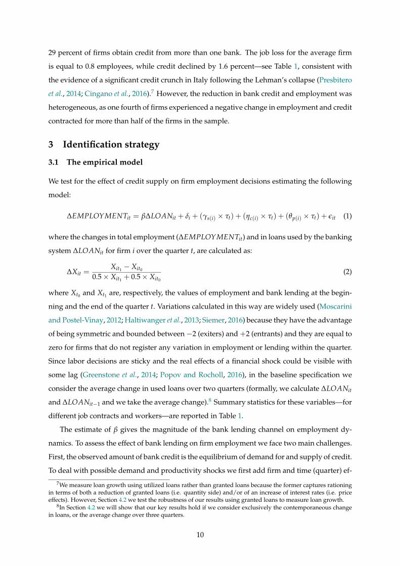
We test for the effect of credit supply on firm employment decisions estimating the following

model:

∆EMPLOYMENTit = β∆LOANit + δi + (γs(i) × τt) + (ηc(i) × τt) + (θp(i) × τt) + εit (1)

where the changes in total employment (∆EMPLOYMENTit) and in loans used by the banking

system ∆LOANit for firm i over the quarter t, are calculated as:

∆Xit =Xit1 − Xit0

0.5 × Xit1 + 0.5 × Xit0

(2)

where Xt0 and Xt1 are, respectively, the values of employment and bank lending at the begin-

ning and the end of the quarter t. Variations calculated in this way are widely used (Moscarini

and Postel-Vinay, 2012; Haltiwanger et al., 2013; Siemer, 2016) because they have the advantage

of being symmetric and bounded between −2 (exiters) and +2 (entrants) and they are equal to

zero for firms that do not register any variation in employment or lending within the quarter.

Since labor decisions are sticky and the real effects of a financial shock could be visible with

some lag (Greenstone et al., 2014; Popov and Rocholl, 2016), in the baseline specification we

consider the average change in used loans over two quarters (formally, we calculate ∆LOANit

and ∆LOANit−1 and we take the average change).8 Summary statistics for these variables—for

different job contracts and workers—are reported in Table 1.

The estimate of β gives the magnitude of the bank lending channel on employment dy-

namics. To assess the effect of bank lending on firm employment we face two main challenges.

First, the observed amount of bank credit is the equilibrium of demand for and supply of credit.

To deal with possible demand and productivity shocks we first add firm and time (quarter) ef-

7We measure loan growth using utilized loans rather than granted loans because the former captures rationingin terms of both a reduction of granted loans (i.e. quantity side) and/or of an increase of interest rates (i.e. priceeffects). However, Section 4.2 we test the robustness of our results using granted loans to measure loan growth.

8In Section 4.2 we will show that our key results hold if we consider exclusively the contemporaneous changein loans, or the average change over three quarters.

10

fects, which allow for firm-specific time invariant demand shifters and for common global

shocks occurring at a quarterly frequency. Then, we saturate the model with more sophisti-

cated industry × quarter (γs(i) × τt) and province × quarter (θp(i) × τt) fixed effects, and with

a set of dummies that vary across quarters and firm class size (micro, small and medium-large

firms, ηc(i) × τt). The degree of granularity of these borrower fixed effects is such that our

identification hinges on the assumptions that: 1) firm unobserved heterogeneity which drives

labor demand (i.e. managerial risk appetite) is time invariant, and 2) all firms operating in the

same 2-digit industry, in the same province, and in the same class size face the same demand

or productivity shock in each quarter. Given that we consider the universe of firms in a rela-

tively homogeneous region, we believe that such granular fixed effects should be sufficient to

isolate time-varying unobserved demand shocks. That said, we run additional robustness test

allowing for more demanding firm cluster×time fixed effects to absorb time-varying borrower

demand shocks, using sector-province-size-quarter fixed effects (see Section 4.2).

Second, bank lending is endogenous to firms’ economic conditions and employment choices,

so that standard OLS estimates are likely to be biased.9 To isolate a credit supply shock from a

lower demand for credit we build on an instrumental variable (IV) approach similar to the one

proposed by Greenstone et al. (2014). We construct a time-varying firm-specific index of credit

supply (CSIit) – discussed in detail in the following section – and we use it as an instrument

for ∆LOANit. In this way, we can measure the firm-level ‘aggregate’ bank lending channel

(Jiménez et al., 2014), which takes into account general equilibrium effects (i.e. the possibility

that firms substitute for credit across banks).

3.2 Credit supply index

To isolate the exogenous component of credit supply we adopt a data-driven approach, bor-

rowed from Greenstone et al. (2014). Specifically, we estimate the following equation that de-

composes the contribution of demand and supply factors to bank lending growth:

∆Lbpst = α + δbt + γpst + εbpst (3)

where the outcome variable ∆Lbpst is the percentage change in outstanding business loans by

bank b, in province p, in sector s at time t; specifically we observe outstanding loans for about

650 banks, 100 provinces (after having excluded those located in Veneto) and main sectors of

9On the one hand, low performing firms can be more likely to demand/receive less credit and to contract thelabor force, inducing an upward bias in the OLS estimates. On the other hand, the OLS could be downward biasedbecause of ‘evergreening’ practices, so that firms under stress would reduce their employment, but at the sametime receive additional credit from their banks (Peek and Rosengren, 2005).

11

activity (agriculture, manufacturing, construction, and private non-financial services)10; γpst is

a set of province-sector-quarter fixed effects that capture the variation in the change of lending

due to province-sector cycles, which we can interpret as broadly measuring local demand;

the bank-time fixed effects δbt represent our parameters of interest and capture (nationwide)

bank lending policies. The identification of both γpst and δbt is guaranteed by the presence

of multiple banks in each province-sector market (i.e. multiple banks exposed to the same

demand) and the presence of each bank in multiple province-sector markets (i.e. multiple

markets exposed to the same bank supply conditions).

We then construct a time-varying firm-specific index of credit supply, aggregating the bank-

specific supply shocks estimated above with the beginning-of-the-period banks’ shares at the

firm level as weights. Specifically, the credit supply for the firm i at time t is:

CSIit = ∑b

wbit0 × δbt (4)

where δbt are the bank-time fixed effects estimated in equation 1and wbit0 is the bank b market

share for firm i at the beginning of the sample period (end-2007).

By construction, CSIit captures the time-varying credit supply at the firm level and its

sources of variability are the substantial heterogeneity in changes in business lending across

banks and the variation in bank market shares across firms. To further convince the reader that

our measure of credit supply is actually correlated with the evolution of credit conditions in

Italy and with bank characteristics we provide a set of stylized facts.

First, we show that, at the nationwide level, the credit supply index mimics quite well the

growth rate of business loans; the correlation is stronger in the first part of the crisis and weaker

in more recent years (Figure 6, panel a); the latter pattern might be due to the prevalence of

demand factors in the second part of the crisis as main drivers of loan growth rate. More in-

terestingly, from a microeconomic point of view, banks applying different conditions in terms

of access to credit are characterized by significant differences in loans dynamics. Specifically,

for each period we divide banks into two groups, depending on whether their estimated credit

supply orientation was below or above the median, and we examine credit patterns for both

groups: as expected, tight banks recorded more negative patterns than ease ones (Figure 6,

panel b). Moreover, the large drop in credit supply conditions from the beginning of the finan-

cial crisis on, was mostly concentrated among large banks (Figure 6, panel c), consistent with

the fact that those banks were more exposed to the liquidity drought in interbank markets.

Finally, the time pattern of our credit supply indicator is also consistent with other aggregate

10Provinces correspond to NUTS 3 Eurostat classification (a geography entity similar to U.S. counties) and, ac-cording to the supervisory authority, they represent the “relevant” market in banking (see also Guiso et al., 2004).

12

indicators measuring the credit supply orientation. Specifically, in panel d) of Figure 6 we plot

the (inverse of) CSI together with: 1) the diffusion index from the ECB Bank Lending Survey

on Italian banks,11 2) the share of rationed firms as reported by a survey on firms maintained

by the Bank of Italy, and 3) a corporate credit rationing indicator developed by Burlon et al.

(2016) using bank-firm matched data. The chart shows that the credit supply index follows

closely the evolution of bank lending standards and the ones of firm financing constraints; the

correlation of the CSI with the three measures of credit constraints varies between 0.5 and 0.6.

Second, our measure of credit supply shows the expected correlation with bank character-

istics. We run a set of bank level regressions on the cross section of banks, taking the average

CSIit over the period 2008-2012 as the dependent variables and a set of bank characteristics

measured at end-2007 as explanatory variables. The worsening in credit supply conditions

was higher for larger banks and those with larger funding gap (measured with the deposit-to-

loan ratio) and with lower capital, consistently with the fact that those banks were likely more

exposed to the liquidity drought in interbank markets and, more generally, to the financial

turmoil (Table 2).

The exogeneity of CSIit relies on the two terms wbit0 and δbt. As the first term, our assump-

tion is that the bank market shares at the firm level, once we have controlled for firm-fixed

effects, are not correlated with the employment trend at the firm level. Though this is a reason-

able assumption, one may still have some concerns. For example, if main banks specialized

in larger firms that were more exposed to the economic cycle (thus experiencing an employ-

ment decrease) and if those same banks also restricted credit supply more than other players,

then a correlation between our credit supply indicator and firm employment growth would

be spurious. In order to address this point we include in the specification sector-quarter and

size-quarter fixed effects. If our parameter of interest is fairly stable we may argue that the ar-

gument discussed above is not an issue in our case. Moreover, as shown in Table 3 on balancing

properties, the exposure to credit shocks at the firm level in our sample period (obtained av-

eraging CSIit over the period 2008-2012) is not significantly correlated (both from a statistical

and economic point of view) to firm size at the beginning-of-the-period.

As far as the second term is concerned, bank-time fixed effects δbt are exogenous by con-

struction since they are purged of unobserved province-sector-quarter factors and it is rather

implausible that unobserved effects at the firm level are able to affect nationwide banks’ lend-

ing policies. Nevertheless, our identification assumption can be violated if banks with negative

11The “diffusion indexes” reflects subjective assessments of the lender on the relative importance of demandand supply factors in explaining the lending patterns. Technically, the diffusion index is the (weighted) differencebetween the share of banks reporting that credit standards have been tightened and the share of banks reportingthat they have been eased.

13

supply shocks were more likely to grant credit to firm that were hit more by the crisis. This

may occur if, for example, bank policies vary across bank characteristics (e.g. size) and the lat-

ter is correlated with firm characteristics (e.g. larger banks grant loans to larger firms). If this is

true and if firm characteristics are correlated with firm employment outcomes—as plausible—

then the instrument will not be orthogonal to the error term in equation 1. Also, one could

argue that, even in the same province-sector cluster, some banks can specialize into lending to

firms with a specific demand for credit, since they rely on different product markets (i.e. large

exporters). In that case, the estimated bank-time fixed effects δbt could capture a demand effect

rather than a pure supply effect. However, summary statistics reported in Table 3 shows that

there is no systematic correlation between the size of the exposure to the credit supply shocks

and a set of firm characteristics, such as size, financial dependence, banking relationships, ge-

ographical location, and sector of activity.12 The first five columns report summary statistics

of firm beginning-of-the-period characteristics by quintile of CSIit, averaged over the period

2008-2012 while the last column simplifies this information reporting the correlation between

these pairs of variables. It turns out that firm characteristics are well balanced with respect to

the average exposure to the credit shock during our temporal window.

Our approach depart from Greenstone et al. (2014) along several dimensions that, in our

view, reinforce the exogeneity and reduce the bias of the indicator.13 First, we translate bank-

time fixed effects at the firm rather than at the county level. This approach reinforces the ex-

ogeneity of the instrument because while one may argue that unobservable shock in a county

may affect (nationwide) lending policies of banks (especially when the local market is suffi-

ciently large with respect to the national credit market of a certain bank), this is less plausible

in case of unobservable shock at the firm level. Second, we strengthen the exogeneity also

excluding the Veneto provinces from equation 1, so that we exclude the effects of demand

and supply factors in this region from the calculation of bank-time fixed effects.14 Third, our

12While the set of observable characteristics does not include some key variables (like the export orientation), itis difficult to think at firm characteristics which are correlated with the credit supply index while being orthogonalto the variables listed in Table 3.

13An alternative identification strategy is the one proposed by Amiti and Weinstein (2016), who identify thebank shocks (i.e. time varying bank fixed effects) through a regression on the dynamic of loans at the firm level,exploiting information from the sub-sample of firms who borrow from multiple banks. However we believe thattheir approach is less suitable for our case since the fraction of firms who have multiple lending relationshipsvaries a lot with firm size: in our data, for example, more than 90 percent of medium and large firms have multiplerelationships in contrast to about 30 percent for micro-firms. Therefore the identification of bank fixed effects witha regression at the firm level is arguably less reliable with our sample that include a large number of micro andsmall firms.

14The exclusion of Veneto provinces from the estimation of bank lending policies leads to the exclusion of onlyone bank (accounting for less than 0.1 percent of loans granted to all firms residing in Veneto), for which we werenot able to estimate the national lending policy. Therefore, this strategy does not affect the representativeness of oursample, while it strongly reinforces the exogeneity of the instrument. It is also worth noting that Veneto representsabout 8 percent of total loans granted by the median bank active in the region.

14

data allows us estimating time-varying bank fixed effects after having controlled for province-

sector-time unobserved factors while Greenstone et al. (2014) control only for counties-time

unobserved factors. This means that we are able to account from bank-specific demand shock

that may occur whenever banks specialize in lending to certain industries and these indus-

tries perform differently from others. Fourth, in Italy government interventions in favor of the

banking system has been very limited, contrarily to what happened in the U.S. and in other

European countries. This implies that the lending policies of the banks were not affected by

constraints imposed by the government as conditions to receive public support and, therefore,

that our estimates are not affected by this potential source of bias.

4 Results

4.1 Main results

To help illustrate the impact of the credit supply, Figure 7 plots the employment patterns for

firms classified in two groups, depending on whether they were exposed over the period 2008-

2012 to tighter or easier lending policies (i.e. CSI below or above the median). More specifically,

plotted values are the residuals (average of the two groups) of a regression of logarithm of

employees on firm and quarter fixed effects, so that residuals are on average equal to zero

and their time patterns shows the dynamics of employment for the two groups. The two lines

suggest that less favorable lending conditions are associated with a decrease in employment

and with a divergent dynamic with respect to firms who experienced a better access to credit.

The following regression tables statistically substantiate this visual evidence.

Table 4 reports the 2SLS robust estimates of the baseline model for the whole sample of

firms, including firm and quarter fixed effects (column 1), and time-varying industry, class

size, and province fixed effects (columns 2 to 4).

The top panel reports the first stage estimates, which show that, as expected, the CSI is

positively associated with the change in used loans and the coefficients is precisely estimated.

The relevance of the instrument is further confirmed by the value of the first-stage F-statistic,

which ranges between 156 and 180, well above the critical value of 10 suggested by Staiger and

Stock (1997).

The second-stage results—reported in the bottom panel—confirm the existing evidence

about the negative effect of a credit supply shock on employment (Chodorow-Reich, 2014; Ben-

tolila et al., 2015), since the change in used loans has a significant and economically large effect

on the variation in employment at the firm level. Comparing the four different specification

shows that adding fixed effects reduces the employment effect of the credit crunch, as they are

15

capturing time-varying borrower-specific demand and productivity shocks. In particular, the

point estimate of the coefficient on ∆LOAN ranges from 0.36 in column 1 to 0.34 when adding

time-varying industry and size fixed effects and finally to 0.25 when time-varying industry,

size and province fixed effects are jointly added in the model (last column).

From now on, we will take the specification of column 4 as our baseline. The point estimate

of the bank lending channel is 0.25, meaning that a 10 percent contraction in bank lending

over two quarters translates into a 2.5 percent reduction in employment. In relative terms, one

standard deviation of the predicted change of used loan explains 15% of the standard deviation

of employment.

In order to have aggregate evidence of the impact, we calculate the share of the change of

employment in our temporal window that can be attributed to the credit crunch, bearing in

mind the caveat that there are general equilibrium effects that cannot be taken into account

when extrapolating microeconomic estimate at the aggregate level (Chodorow-Reich, 2014).

In our case, for example, results are obtained conditional on firms having bank debt, so that

our estimates are silent on possible demand shift to firms non depending on bank credit. In

our sample, the credit extended to firms diminishes by 1.6 percent while employment by 0.8

percent (see Table 1), both on a quarterly base. Since our preferred estimate of the elasticity

of employment to credit is computed cumulating the effect over two quarters we can assume

that the quarterly impact is roughly half. With simple algebra, it is easy to show that the credit

drop attributable to the lending supply orientation over the period 2008-2012 explained about

one fourth of the employment loss.

Overall our results indicate a quite large effect of the credit crunch on employment. These

findings are also roughly comparable, in magnitude, to those estimated by Bentolila et al. (2015)

for Spain and Chodorow-Reich (2014) for the U.S. However, compared to these exercises—

which are generally focused on medium and large enterprises—our analysis is less subject

to external validity concerns related to the representativeness of the data, since our sample

include micro and small firms and covers almost the universe of private non-financial firms

and employment of the region.15

4.2 Robustness

We test the robustness of our baseline results running a battery of additional tests. Results are

showed in Table 5. First, to address the concerns that our set of borrower fixed effects might

not fully absorb demand and productivity shock, we saturate our model with more demand-

15The average firm size is nearly 3,000 in Chodorow-Reich (2014) and about 25 in Bentolila et al. (2015), while inour case is around 6 as we are able to observe the universe of firms.

16

ing fixed effects. We start by interacting the quarter dummies with more restrictive borrower

cells (industry × size, industry × province, and province × size), allowing for time-varying

demand to be the same not only across industries, class size and provinces, but also withing

their two-way combinations (columns 1-3). Then, in the spirit of recent works that has to deal

with a prevalence of single bank-firm relationships (Abuka et al., 2015; Auer and Ongena, 2016;

Degryse et al., 2016), we fully saturate the model with firm cluster×time—where the firm clus-

ter is composed by all firms in the same industry, province, and class size—which are as close

as we can get to quarterly firm fixed effects (column 4). Interestingly, the coefficient on ∆LOAN

is not only precisely estimated, but it remains remarkably stable at around 0.25 in columns 1-3.

The inclusion of the four-way fixed effects only marginally attenuates the magnitudes of the

estimated credit effect on employment, suggesting that there is no additional unobserved het-

erogeneity driving our estimates. Hence, we will use the baseline set of fixed effects showed

in Table 4 (column 4) throughout the rest of the analysis.

In columns 5 we show that our results are robust to clustering the standard errors to allow

for intra-group correlation in the error term at the province-industry-class size level: the stan-

dard error only marginally increases while the coefficient of interest remains highly significant.

Similar results (available from the authors upon request) are obtained using different levels of

clustering.

In column 6 we restrict the sample to firms which have a total debt above 75,000 euros

throughout the entire sample period, to avoid potential biases arising from the change in the

threshold in our sample period. We find that the coefficient on ∆LOAN slightly increases to

0.38, but it is still precisely estimated.

One could argue that employment dynamics could be affected also by the housing net worth

channel, which can compress demand because of a direct wealth effect or tighter borrowing

constraints, through a fall in collateral values. This channel has been responsible for a sig-

nificant drop in employment in the U.S. during the financial crisis (Adelino et al., 2015; Mian

and Sufi, 2014) and it could also be important in our set-up, because of high home ownership

rates in Italy (76 percent of households own their house in Veneto) and because, differently

from most of the literature, we deal with entrepreneurs of micro firms, who are likely to post

their house as a collateral for business loans. However, the housing boom-and-bust cycle in

Italy has been quite limited, and even more so in Veneto (Figure A1 in the annex). In any case,

to further avoid any confounding factor affecting our estimates, we add time-varying house

prices at the municipality level and we find that the inclusion of house prices does not change

the coefficients on the loan variable (column 7).

17

Finally, we do some robustness exercise on the ∆LOAN variable. Rather than taking the

average change in used loans over two quarters, in columns 7 and 8 we consider exclusively

the contemporaneous change (at time t) and the average changes over three quarters (t, t − 1,

and t − 2), respectively.16 We still find evidence that a contraction in the credit supply reduces

employment and, as expected, the effect is smaller when looking at the contemporaneous ef-

fects and increasing allowing for more lags. In our final exercise we measure bank lending not

in terms of used loans but as granted loans: the coefficient on lending is larger than the one on

used loans, but it remains statistically significant.

4.3 Job contract heterogeneity

As a second step of our analysis we zoom in on the composition of the labor force adjustment,

to assess in which way firms changed their workforce. Given that we cannot reconstruct the

stock of workers by type of contracts and by worker characteristics, we estimate equation 1

taking as dependent variables the quarterly change of employment at the firm level for a given

job or worker characteristic, scaled by the average stock of all firm’s workers over the quarter.17

Therefore, differently from the baseline model, the dependent variable is not a growth rate but

a contribution to the aggregate (at the firm level) growth rate. This means that the estimated

coefficients cannot be interpreted as elasticities, but they need to be scaled by the relative share

of the job contracts/workers. Lacking that information in our sample, we use the aggregates

shares at the regional level, as compiled by from the National Institute of Statistics (‘Labour

Force Survey’), in order to provide an economic interpretation of our findings, see Table 1.

At first, we consider open-ended and temporary contracts—which include fixed term di-

rect hires, project workers, temporary agency workers, trainees and apprentices, and seasonal

workers—to test whether firms reacted to more binding financing constraints reducing the use

of temporary contracts more than open-ended ones (Table 6, top-left panel). We find that the

employment adjustment happened primarily through the lay-off (or non-renewal) of tempo-

rary contracts. The coefficient on ∆LOAN is positive and statistically significant for both type

of contracts, even though given that temporary contracts account for slightly more than one

tenth of total contracts in the workforce (Table 1), the economic effect of the credit contraction

is much stronger for temporary than open-ended contracts, since changes in employment due

to the former account for 73 percent of the total effect (0.185/0.252 = 0.73).

This result is consistent with a growing body of literature pointing to endogenous selec-

16The construction of the instrument is modified accordingly.17In other words, the dependent variable is calculated as the ratio between the job flows for a given category of

contracts or workers—which we retrieve from PLANET—and the average stock of total workers (0.5× Xit1 + 0.5×Xit0 , as defined at the denominator of equation 2).

18

tion and lower human capital accumulation for temporary workers. In particular, temporary

workers accumulate less skills—especially firm-specific skills—for both a mechanical reason

(shorter seniority leading to less learning-by-doing) and a strategic decision by firms, which

provide less on-the-job training. If wages display downward rigidities, firms are likely to

reduce their temporary workforce first. Moreover, temporary workers suffer more than open-

ended ones simply because they are easier to be dismissed. Indeed, recourse to temporary

contracts is known to be more cyclical than the use of open-ended contracts (García Serrano,

1998; Goux et al., 2001). Because firms do not have to pay dismissal costs upon termination of

temporary contracts, they typically employ temporary workers as a buffer stock, to deal with

expected or unexpected fluctuations in demand or in financial conditions.

To better understand the employment dynamics following the credit crunch, we differ-

entiate between inflows and outflows and we find that our results are mostly driven by the

dynamics of outflows, which are higher for firms more exposed to the credit supply shock (Ta-

ble 6, bottom-left panel). Then, within outflows, we differentiate across the possible reasons

of the exit and we find evidence that outflows are exclusively due to non-renewal of expired

contracts, while there is no evidence that the adjustment works through dismissal or quit (Ta-

ble 6, top-right panel). Finally, we look at the transitions across job contracts, considering

both contract type and time schedule. We find evidence that firms more exposed to negative

credit shocks are are less likely to transform temporary contracts into open-ended ones, while

it seems that financing constraints do not affect firm policies in terms of transition between

part-time and full-time jobs (Table 6, bottom-right panel).

4.4 Worker heterogeneity

Looking at the workers’ characteristics, we first differentiate across three levels of education—

low (at most compulsory education), medium (at most upper secondary education), and high

(tertiary education), based on the ISCED classification—and we observe that firms which have

experienced a reduction in the supply of credit reacted reducing the employment of low- and

medium-educated workers, while there is no effect for the highly educated ones (Table 7, top

panel). In particular, using the relative shares reported in Table 1, the elasticity of employment

to credit supply for low-educated workers is higher than the average and equal to 0.36 (=

0.140/0.387). In other words, changes in employment within low-educated workers account

for 56 percent of the total effect of ∆LOAN (0.140/0.252 = 0.56), even though low-educated

workers account for less than 40 percent of the workforce.

Education may not perfectly overlap with the skill content of jobs; moreover, administra-

19

tive data may record with errors self-reported information as the level of education. Therefore

we replicate the analysis by skill level directly looking at the skill content of each occupation

(Table 7, bottom panel).18 The results based on this different measure of skill level are very

similar to those based on the education level. The differential effect across skills or education

is consistent with the theory of skill upgrading, which indicates that, in a downturn, firms

want to dismiss less skilled, less profitable workers first (Reder, 1955).

Then, we assess whether firms adjusted their labor force differentiating across workers,

depending on their gender, age, and nationality. Our results—showed in Table 8—indicate

that the employment effect in response to a reduction in the supply of credit is concentrated

among women, foreign and younger workers. In particular, female workers represent around

40 percent of total employment, but they account for 70 percent of the total change in em-

ployment. Similarly, foreign workers are less the 10 percent of the labor force, but their em-

ployment dynamics explains more than 30 percent of the total change in employment.19 There

is also evidence that younger people are more likely to be hit by consequence of the credit

crunch, consistent with recent evidence showing that young workers are the most affected

during recessions (Forsythe, 2016). The under 30 contribute to more than a third of the overall

employment effect, even though they represent less than 20 percent of the workforce.20

Finally, in Table 9 we take advantage of the several dimensions in which we can slice our

data to measure the impact of the credit crunch on employment, conditional both on contract

type and worker education. We find that indeed firms adjusted their labor force in response

to a contraction in the supply of credit reducing temporary contracts and dismissing low and

medium-educated workers. By contrast, highly-educated workers have been able to insulate

themselves, even if hired with a temporary contracts. This result is consistent with the hy-

pothesis that low-skilled individuals suffer most from recessions—possibly because of lower

training and hiring costs compared to more educated workers—and with the empirical evi-

dence on Germany discussed by Hochfellner et al. (2016). Overall, the results of our analysis

indicates that the combination of low-education and temporary contract identifies the profile

18Specifically, we look at the ISCO classification of occupations and we consider low-skilled those employed inelementary occupations and services and sales workers; clerical support workers, craft and related trades workersand plant and machine operators, and assemblers have an intermediate level of skills; finally, managers, profes-sionals and technicians are highly-skilled workers.

19We cannot exclude that some of the penalty for foreign workers comes from sheer discrimination. For instance,it has been documented that economic downturns favor racial prejudice and lead to worse labor market outcomesfor minorities (Johnston and Lordan, 2016).

20The recognition that unemployment has important distributional consequences goes back at least to Tobin(1972). In their comprehensive assessment of employment and unemployment patterns across U.S. business cycles,Hoynes et al. (2012) show that men, non-whites, youth, and less educated workers show higher sensitivity toeconomic conditions. These differences in cyclicality appear to be very stable over time, from the late 1970s to theGreat Recession.

20

of workers who has been hit by the credit crunch, while high education makes irrelevant the

difference between temporary and open-ended contracts.

4.5 Firm heterogeneity

Finally, we explore possible heterogeneous effect across different firms.21 First, we are inter-

ested in assessing whether the employment response to a credit supply shock differ across

firm size, given that SMEs are more likely to be financially constrained, have limited access

to alternative sources of external finance, and depend more on bank credit than large firms,

so that the real effects of credit shocks is likely to be larger (Beck et al., 2008; Presbitero et al.,

2014; Cingano et al., 2016). In our data the reliance on bank financing also differs across firm

size (Figure 3). The estimation of equation 1 for the three sub-samples of micro (less then 10

employees), small (between 10 and 49 employees) and medium-large (50 or more employees)

firms shows that our results hold only for micro and small firms, consistent with what found

by Bottero et al. (2015) on a sample of Italian firms over a similar time period (Table 10, left

panel). By contrast, the coefficient on ∆LOAN is not statistically significant in the sample of

medium-large firms: the coefficient is positive but imprecisely estimated, and the first-stage F-

statistic suggests that there are weak identification problems, possible due to the small sample

size and to the capacity of large firms to negotiate with banks about credit terms, while small

firms are more likely to be exposed to (nationwide) banks’ credit policies.

When splitting our sample across sectors, we find that employment reacts to credit shocks

only in services, while there is no evidence that industrial firms reduce employment in re-

sponse to a credit crunch (Table 10, right panel). In our view, the negligible impact of financing

constraints on employment patterns in the industrial sector may depend on the wider use of

open-ended contracts and on the larger firm size (and, therefore, on the lower dependence on

bank credit) of industrial firms compared to the one in the service sector.22

To shed light on the mechanisms through which financial shocks could affect employment

21We report all results using sub-samples, but we obtain similar findings estimating the equation 1 on the wholesample and interacting ∆LOAN by firm characteristics (size, sector and a dummy for multiple bank relationships).

22One may argue that the sources of heterogeneity discussed so far have a strong overlap, meaning that we areobserving the same firm employment decision (the worker which has been dismissed) from different angles (aworker of small firm in the service sector, with a temporary contract and low education). To reassure the skepticalreader that job contracts and education really matters for employment outcomes during a credit crunch over andabove the effect of firm characteristics, we run our model on different sub-samples according to sectors and firmsize. Table A1—reported in the annex—shows that the effect of the credit crunch on temporary contracts holdseven within firms in services, as well as within micro and small firms. The adjustment on open-ended contract,instead is generally not statistically significant and—when it is, like within micro firms—the size of the elasticityis rather small. Similarly, annex Table A2 confirms that the effect of the credit crunch on the occupation of lesseducated workers survives within micro and small firms and in the service sector. Similarly, it is worth notingthat also differences across age, gender, and nationality are also valid within sectors and firm class size (results notshown but available upon request).

21

decisions we exploit a set of firms’ financial characteristics available in our data. If banks play

a crucial role in addressing firms’ financing needs, then a sudden drop of credit supply should

impact disproportionately more on firms relying more on bank credit, having less flexibility in

the use of granted credit lines, and having weaker relationships with their lenders.

First, we examine whether firms that were more indebted at the beginning of our sample

period suffered more from the tightening of credit conditions. We consider a firm as more

(less) exposed to bank credit if its debt per employee is higher (lower) than the one of similar

firms (i.e. we compare firms in the same industry and class size). This choice makes it possible

to account for different production functions across industries and to avoid having results that

overlap with those showed before. We find that employment reacts relatively more to credit

supply restrictions in firms that are more dependent on bank credit (Table 11, left panel). Sec-

ond, we find that the elasticity of employment to credit is higher for firms that at the beginning

of our sample period were using granted credit lines more intensively (Table 11, middle panel).

Finally, we explore the possibility that the extent of job disruption following a credit supply

shock depends on the strength of the bank-firm relationship. We consider the number of bank

relationships, differentiating between firms which borrow exclusively from one bank during

the sample period and firms with multiple lending banks. We find positive and significant elas-

ticities in the two sub-samples, even though the point estimate is larger for firms with multiple

bank relationships (Table 11, right panel), suggesting that weaker lending relationships expose

firms relatively more to the credit crunch. Thus, our results lend support to recent evidence

showing that Italian firms that borrowed from fewer banks suffered a smaller contraction of

bank credit and a lower increase in lending rates following the Lehman Brothers’ bankruptcy

(Gobbi and Sette, 2014; Gambacorta and Mistrulli, 2014).

5 Extensions

To have a better sense of which are the firms that contract employment more in response to a

financial shock in this section we show a set of additional results obtained on a sub-sample of

firms for which it is possible to obtain and match balance-sheet information. [discuss cerved

data] While the availability of balance-sheet information allows for a better understanding of

the mechanisms through witch a financial shock propagates to the real economy, the match

with the Cerved data comes at the non-trivial costs of loosing one of the key feature of our

analysis—the coverage of the universe of firms, including small and micro enterprises—and

moving from a quarterly to a yearly frequency in the empirical analysis. However, moving

from the universe of firms to the Cerved sub-sample does not significantly alter our baseline

22

results and the coefficient on ∆LOAN is slightly higher in the latter sample than in the whole

one (Table ??).

5.1 Firm heterogeneity

5.2 Capital accumulation and value added

6 Conclusions

The recent literature on finance and labor has showed that firms reduce employment in re-

sponse to a credit crunch. Our analysis takes advantage of a novel dataset on job contracts and

labor market flows for the universe of firms in a large Italian region to look at the within-firm

personnel dynamics and identify which kind of workers is more likely to be laid off, depend-

ing on firm, individual, and job contract characteristics. To identify the employment effect of

the credit crunch, our identification strategy relies of loan level data to build a firm-specific

time-varying measure of credit supply restriction and to control for time-varying demand and

productivity shocks using a granular set of borrower fixed effects.

Our baseline results confirm that financially constrained firms reduced employment and

the point estimate indicate that the elasticity of employment to a credit supply shock is 0.25.

The aggregate effect, based on our estimates, is economically meaningful since the contraction

in bank lending is able to explain about one fourth of the reduction in employment. In addi-

tion, we also show that the adjustment has been differentiated across firms, workers and job

contracts. In particular, the credit crunch has mainly affected less educated and less skilled

workers with temporary contracts, suggesting that firms have adjusted to the credit supply

shock in a way which is consistent with a skill upgrading of the labor force, even though this

strategy has been significantly affected by labor market regulation. Finally, we show that high

financial dependence and weak bank-firm relationships increase firms’ vulnerability and ex-

acerbate the (negative) impact of the credit crunch on employment.

23

References

ABUKA, C., ALINDA, R. K., MINOIU, C., PRESBITERO, A. et al. (2015). Monetary Policy in a De-

veloping Country; Loan Applications and Real Effects. IMF Working Paper 15/270, International

Monetary Fund, Washington DC.

ADELINO, M., SCHOAR, A. and SEVERINO, F. (2015). House prices, collateral, and self-

employment. Journal of Financial Economics, 117 (2), 288–306.

AMITI, M. and WEINSTEIN, D. E. (2011). Exports and Financial Shocks. The Quarterly Journal

of Economics, 126 (4), 1841–1877.

— and — (2016). How Much do Idiosyncratic Bank Shocks Affect Investment? Evidence from

Matched Bank-Firm Data. Journal of Political Economy, Forthcoming.

AUER, R. and ONGENA, S. (2016). The Countercyclical Capital Buffer and the Composition of

Bank Lending, unpublished.

BECK, T., DEMIRGÜÇ-KUNT, A. and MAKSIMOVIC, V. (2008). Financing patterns around the

world: Are small firms different? Journal of Financial Economics, 89 (3), 467 – 487.

BENMELECH, E., BERGMAN, N. K. and SERU, A. (2015). Financing labor, National Bureau of

Economic Research.

BENTOLILA, S., JENSEN, M., JIMENEZ, G. and RUANO, S. (2015). When Credit Dries Up: Job

Losses in the Great Recession. Working Paper Series 4528, CESifo.

BERG, T. (2016). Got rejected? Real effects of not getting a loan. ECB Working Paper 1960, European

Central Bank.

BOERI, T., GARIBALDI, P. and MOEN, E. R. (2013). Financial Shocks and Labor: Facts and

Theories. IMF Economic Review, 61 (4), 631–663.

BOTTERO, M., LENZU, S. and MEZZANOTTI, F. (2015). Sovereign debt exposure and the bank

lending channel: impact on credit supply and the real economy. Working Paper 1032, Bank of

Italy.

BURLON, L., FANTINO, D., NOBILI, A. and SENE, G. (2016). The quantity of corporate credit

rationing with matched bank-firm data. Working Papers 1058, Bank of Italy, Rome.

CAGGESE, A. and CUÑAT, V. (2008). Financing constraints and fixed-term employment con-

tracts. Economic Journal, 118 (533), 2013–2046.

CHODOROW-REICH, G. (2014). The employment effects of credit market disruptions: Firm-

level evidence from the 2008–9 financial crisis. Quarterly Journal of Economics, 129 (1), 1–59.

CINGANO, F., MANARESI, F. and SETTE, E. (2016). Does Credit Crunch Investments Down?

New Evidence on the Real Effects of the Bank-Lending Channel. Review of Financial Studies,

Forthcoming.

24

DEGRYSE, H., DE JONGHE, O., JAKOVLJEVIC, S., MULIER, K. and SCHEPENS, G. (2016). The

Impact of Bank Shocks on Firm-level Outcomes and Bank Risk-Taking, Available at SSRN

2788512.

DEVICIENTI, F., MAIDA, A. and SESTITO, P. (2007). Downward Wage Rigidity in Italy: Micro-

Based Measures and Implications. Economic Journal, 117 (524), F530–F552.

DUYGAN-BUMP, B., LEVKOV, A. and MONTORIOL-GARRIGA, J. (2015). Financing constraints

and unemployment: Evidence from the Great Recession. Journal of Monetary Economics, 75,

89–105.

FABIANI, S., LAMO, A., MESSINA, J. and ROOM, T. (2015). European firm adjustment during

times of economic crisis. Working Paper 1778, European Central Bank.

FORSYTHE, E. (2016). Why Don’t Firms Hire Young Workers During Recessions?, University

of Illinois.

GAMBACORTA, L. and MISTRULLI, P. E. (2014). Bank Heterogeneity and Interest Rate Setting:

What Lessons Have We Learned since Lehman Brothers? Journal of Money, Credit and Bank-

ing, 46 (4), 753–778.

GARCÍA SERRANO, C. (1998). Worker turnover and job reallocation: the role of fixed-term

contracts. Oxford Economic Papers, (50), 709–725.

GOBBI, G. and SETTE, E. (2014). Do firms benefit from concentrating their borrowing? evi-

dence from the great recession. Review of Finance, 18 (2), 527–560.

GOUX, D., MAURIN, E. and PAUCHET, M. (2001). Fixed-term contracts and the dynamics of

labour demand. European Economic Review, (45), 533–552.

GREENSTONE, M., MAS, A. and NGUYEN, H.-L. (2014). Do Credit Market Shocks affect the Real

Economy? Quasi-Experimental Evidence from the Great Recession and ‘Normal’ Economic Times.

NBER Working Papers 20704, National Bureau of Economic Research.

GUISO, L., SAPIENZA, P. and ZINGALES, L. (2004). Does Local Financial Development Matter?

Quarterly Journal of Economics, 119 (3), 929–969.

GURIEV, S. M., SPECIALE, B. and TUCCIO, M. (2016). How do regulated and unregulated labor

markets respond to shocks? Evidence from immigrants during the Great Recession. CEPR Discus-

sion Paper 11403, Center for Economic Policy Research, London.

HALTENHOF, S., LEE, S. J. and STEBUNOVS, V. (2014). The credit crunch and fall in employ-

ment during the great recession. Journal of Economic Dynamics and Control, 43, 31–57.

HALTIWANGER, J., JARMIN, R. S. and MIRANDA, J. (2013). Who creates jobs? Small versus

large versus young. Review of Economics and Statistics, 95 (2), 347–361.

HERSHBEIN, B. and KAHN, L. B. (2016). Do Recessions Accelerate Routine-Biased Technological

25

Change? Evidence from Vacancy Postings. Working Paper 16-254, Upjohn Institute.

HOCHFELLNER, D., MONTES, J., SCHMALZ, M. and SOSYURA, D. (2016). Winners and Losers

of Financial Crises: Evidence from Individuals and Firms, university of Michigan.

HOYNES, H., MILLER, D. L. and SCHALLER, J. (2012). Who suffers during recessions? Journal

of Economic Perspectives, (3), 27–48.

JIMÉNEZ, G., MIAN, A. R., PEYDRO, J.-L. and SAURINA, J. (2014). The Real Effects of the Bank

Lending Channel, Available at SSRN: http://ssrn.com/abstract=1674828.

JOHNSTON, D. W. and LORDAN, G. (2016). Racial prejudice and labour market penalties dur-

ing economic downturns. European Economic Review, (84), 57–75.

MIAN, A. and SUFI, A. (2014). What Explains the 2007–2009 Drop in Employment? Economet-

rica, 82 (6), 2197–2223.

MOSCARINI, G. and POSTEL-VINAY, F. (2012). The contribution of large and small employers

to job creation in times of high and low unemployment. American Economic Review, 102 (6),

2509–2539.

PAGANO, M. and PICA, G. (2012). Finance and employment. Economic Policy, 27 (69), 5–55.

PARAVISINI, D., RAPPOPORT, V., SCHNABL, P. and WOLFENZON, D. (2015). Dissecting the

Effect of Credit Supply on Trade: Evidence from Matched Credit-Export Data. Review of

Economic Studies, 82 (1), 333–359.

PEEK, J. and ROSENGREN, E. S. (2005). Unnatural selection: perverse incentives and the mis-

allocation of credit in Japan. American Economic Review, 95, 1144–1166.

POPOV, A. and ROCHOLL, J. (2016). Do Credit Shocks Affect Labor Demand? Evidence from

Employment and Wages during the Financial Crisis. Journal of Financial Intermediation, Forth-

coming.

PRESBITERO, A. F., UDELL, G. F. and ZAZZARO, A. (2014). The home bias and the credit

crunch: A regional perspective. Journal of Money, Credit, and Banking, 46 (s1), 53–85.

REDER, M. W. (1955). The theory of occupational wage differentials. The American Economic

Review, (45), 833–852.

SIEMER, M. (2016). Employment Effects of Financial Constraints During the Great Recession,

Board of Governors of the Federal Reserve System.

STAIGER, D. and STOCK, J. H. (1997). Instrumental variables regression with weak instru-

ments. Econometrica, 65 (3), 557–586.

TOBIN, J. (1972). Inflation and unemployment. American Economic Review, (62), 1–18.

26

Figures

Figure 1: External validity: firm distribution across size and sectors in Veneto and Italy

0

20

40

60

% o

f firm

s in

eac

h fir

m s

ize

clas

s (#

em

ploy

ees)

Italy Veneto

0-1 2

3-5

6-9

10-4

9

50-2

49

> 25

0

0-1 2

3-5

6-9

10-4

9

50-2

49

> 25

0

(a) Distribution of firms across size

0 5 10 15 20 25% of firms by sector of economic activity

Vene

toIta

ly

TransportationITC

Support servicesEducation and Health

Water & EnergyMining

ConstructionTrade

Sci-techManufacturing

Finance & Real estateAccomodation

Arts and personal servicesOther service

AgricultureTransportation

ITCSupport services

Education and HealthWater & Energy

MiningConstruction

TradeSci-tech

ManufacturingFinance & Real estate

AccomodationArts and personal services

Other serviceAgriculture

(b) Distribution of firms across sectors

Notes: elaborations on ISTAT data (census 2011).

Figure 2: External validity: bank penetration and lending in Veneto and Italy

50

60

70

80

90

Bran

ches

per

100

,000

inha

bita

nts

VeronaVicenzaBelluno Treviso Venice Padua Rovigo North Italy

(a) Financial development

-.02

-.01

0

.01

.02

.03

Bank

loan

gro

wth

to n

onfin

anci

al c

orpo

ratio

ns (q

-o-q

)

2008:Q1 2008:Q4 2009:Q3 2010:Q2 2011:Q1 2011:Q4 2012:Q3

Italy Veneto

(b) Loans growth

Notes: elaborations on data from Bank of Italy.

27

Figure 3: Bank financing in Italy across firm size

0

10

20

30

40

50

% o

f firm

s us

ing

cred

it fo

r fina

ncin

g

Euro area ItalyAll Micro SME All Micro SME

Bank loans Bank overdraft, credit lines

(a) Bank credit (Average 2009-2012, SAFE)

0

50

100

150

Deb

t per

em

ploy

eeMicro (<10) Small (10-49) Medium-large (>49)

(b) Firms’ indebtedness (our data)

Notes: elaborations on data from the Survey on the Access to Finance of Enterprises (SAFE, European Central Bank), Bank ofItaly, PLANET, and ASIA. Debt per employee is measured in thousands of euro.

Figure 4: Sample representativeness, comparison with the Census

0

20

40

60

80

100

Micro (<10) Small (10-49) Medium-large (>49)

Our sample Census 2011

(a) Firms’ distribution (%)

0

10

20

30

40

50

Micro (<10) Small (10-49) Medium-large (>49)

Our sample Census 2011

(b) Employees’ distribution (%)

Notes: elaborations on data from ISTAT (2011 census), PLANET, and ASIA.

28

Figure 5: Sample representativeness, dynamics of firms and employment

1480000

1500000

1520000

1540000

1560000

Num

ber o

f em

ploy

ees

398000

399000

400000

401000

402000

403000

Num

ber o

f firm

s

2008:Q4 2009:Q4 2010:Q4 2011:Q4 2012:Q4

Number of firms Number of employees

(a) Sample, non-financial private sector (deseasonalizeddata)

1550000

1600000

1650000

1700000

Num

ber o

f em

ploy

ees

450000

455000

460000

465000

Num

ber o

f firm

s

2008:Q1 2008:Q4 2009:Q3 2010:Q2 2011:Q1 2011:Q4 2012:Q3

Number of firms Number of employees

(b) Universe, total economy (Source: ISTAT, RFL)

Notes: elaborations on data from PLANET, ASIA and ISTAT (‘Labour Force Survey’).

29

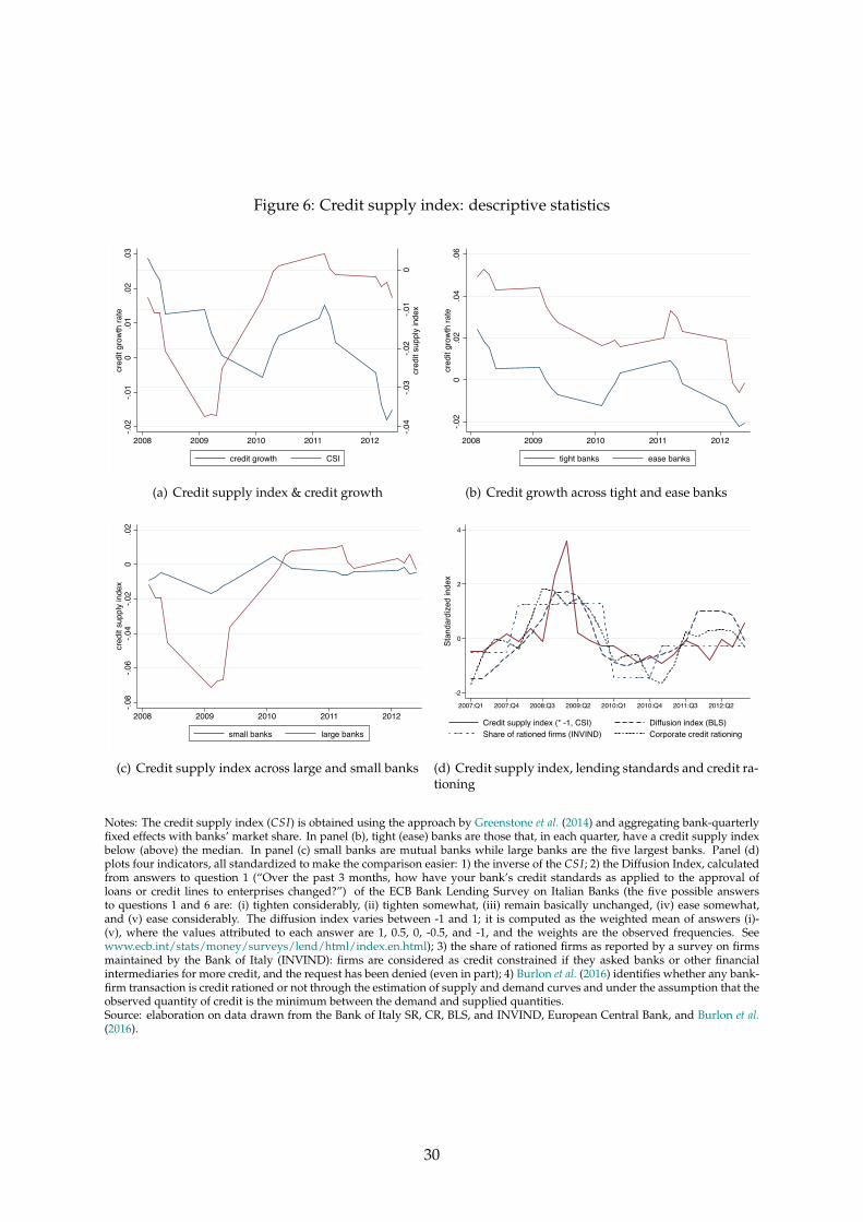
Figure 6: Credit supply index: descriptive statistics

-.04

-.03

-.02

-.01

0cr

edit

supp

ly in

dex

-.02

-.01

0.0

1.0

2.0

3cr

edit

grow

th ra

te

2008 2009 2010 2011 2012

credit growth CSI

(a) Credit supply index & credit growth

-.02

0.0

2.0

4.0

6cr

edit

grow

th ra

te2008 2009 2010 2011 2012

tight banks ease banks

(b) Credit growth across tight and ease banks

-.08

-.06

-.04

-.02

0.0

2cr

edit

supp

ly in

dex

2008 2009 2010 2011 2012

small banks large banks

(c) Credit supply index across large and small banks

-2

0

2

4

Stan

dard

ized

inde

x

2007:Q1 2007:Q4 2008:Q3 2009:Q2 2010:Q1 2010:Q4 2011:Q3 2012:Q2

Credit supply index (* -1, CSI) Diffusion index (BLS)Share of rationed firms (INVIND) Corporate credit rationing

(d) Credit supply index, lending standards and credit ra-tioning

Notes: The credit supply index (CSI) is obtained using the approach by Greenstone et al. (2014) and aggregating bank-quarterlyfixed effects with banks’ market share. In panel (b), tight (ease) banks are those that, in each quarter, have a credit supply indexbelow (above) the median. In panel (c) small banks are mutual banks while large banks are the five largest banks. Panel (d)plots four indicators, all standardized to make the comparison easier: 1) the inverse of the CSI; 2) the Diffusion Index, calculatedfrom answers to question 1 (“Over the past 3 months, how have your bank’s credit standards as applied to the approval ofloans or credit lines to enterprises changed?”) of the ECB Bank Lending Survey on Italian Banks (the five possible answersto questions 1 and 6 are: (i) tighten considerably, (ii) tighten somewhat, (iii) remain basically unchanged, (iv) ease somewhat,and (v) ease considerably. The diffusion index varies between -1 and 1; it is computed as the weighted mean of answers (i)-(v), where the values attributed to each answer are 1, 0.5, 0, -0.5, and -1, and the weights are the observed frequencies. Seewww.ecb.int/stats/money/surveys/lend/html/index.en.html); 3) the share of rationed firms as reported by a survey on firmsmaintained by the Bank of Italy (INVIND): firms are considered as credit constrained if they asked banks or other financialintermediaries for more credit, and the request has been denied (even in part); 4) Burlon et al. (2016) identifies whether any bank-firm transaction is credit rationed or not through the estimation of supply and demand curves and under the assumption that theobserved quantity of credit is the minimum between the demand and supplied quantities.Source: elaboration on data drawn from the Bank of Italy SR, CR, BLS, and INVIND, European Central Bank, and Burlon et al.(2016).

30

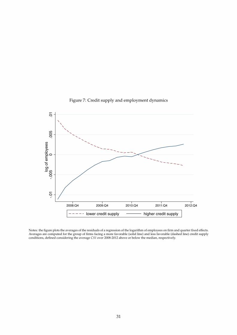
Figure 7: Credit supply and employment dynamics

-.01

-.005

0.0

05.0

1lo

g of

em

ploy

ees

2008:Q4 2009:Q4 2010:Q4 2011:Q4 2012:Q4

lower credit supply higher credit supply

Notes: the figure plots the averages of the residuals of a regression of the logarithm of employees on firm and quarter fixed effects.Averages are computed for the group of firms facing a more favorable (solid line) and less favorable (dashed line) credit supplyconditions, defined considering the average CSI over 2008-2012 above or below the median, respectively.

31

Tables

Table 1: Summary statistics

The table reports the summary statistics for ∆EMPLOYMENT for all workers and for different characteristics of contracts andworkers, for the average change in firm borrowing over two quarters (∆LOAN), and for the credit supply index (CSI). Thesample is the one used in the empirical analysis, made by the universe of firms, conditional on having bank debt. The changein employment for temporary contracts includes fixed term direct hires, project workers, temporary agency workers, traineesand apprentices, and seasonal workers. Education level are defined as low (at most compulsory education), medium (at mostupper secondary education), and high (tertiary education) education, based on the ISCED classification. The skill content of eachoccupation is defined as low (elementary occupations and services and sales workers), medium (clerical support workers, craftand related trades workers and plant and machine operators, and assemblers) and high (managers, professionals and technicians),based on the ISCO classification. The last column report the share of employment at the beginning of the period (end 2007) fordifferent characteristics of contract and workers: these data are taken from the ‘Labour Force Survey’ of the National Institute ofStatistics.

Variable Mean St. Dev. Share in totalemployment(%)

∆EMPLOYMENT - Total -0.0079 0.2050 100.0∆EMPLOYMENT - Open-ended -0.0055 0.1240 88.7∆EMPLOYMENT - Temporary -0.0024 0.1657 11.3∆EMPLOYMENT - Under 30 -0.0001 0.1040 17.9∆EMPLOYMENT - Over 30 -0.0078 0.1620 82.1∆EMPLOYMENT - Male -0.0047 0.1390 59.9∆EMPLOYMENT - Female -0.0032 0.1330 40.1∆EMPLOYMENT - Italian -0.0058 0.1720 91.4∆EMPLOYMENT - Foreign -0.0021 0.0912 8.6∆EMPLOYMENT - Low-education -0.0047 0.1340 38.7∆EMPLOYMENT - Medium-education -0.0025 0.1190 48.0∆EMPLOYMENT - High-education -0.0004 0.0528 13.3∆EMPLOYMENT - Low-skill -0.0022 0.1370 15.2∆EMPLOYMENT - Medium-skill -0.0048 0.1270 49.3∆EMPLOYMENT - High-skill -0.0009 0.0664 35.5

∆LOAN -0.0157 0.3130 .CSI -0.0085 0.0404 .

32

Table 2: Credit supply and bank heterogeneity

The table reports the results of a set of OLS regressions at the bank level (in cross section) in which the dependent variable is theaverage credit supply index (CSI) at the bank level over the sample period 2008-2012 and the explanatory bank-level variablesare measured as of end-2007. For the definition of CSI see Section 3.2 and equation 4. Bank size is measured by the logarithmof total bank assets; the funding gap is measured by the loans-to-deposits ratio; Tier 1 capital ratio is defined as Tier 1 capitalover risk-weighted assets; and the share of NPLs is the ratio of non-performing loans over total loan. Robust standard errors inparentheses; *** p<0.01, ** p<0.05, * p<0.1.

Dep. Var.: CSI at the bank level (average 2008-2012)

Bank size -0.0047*** -0.0014**(0.0009) (0.0007)

Funding gap -0.0102*** -0.0085***(0.0018) (0.0017)

Tier 1 capital ratio 0.0470*** 0.0383***(0.0073) (0.0074)

Share of NPLs -0.0237 -0.0494(0.0388) (0.0365)

Observations 536 536 536 536 536R2 0.084 0.113 0.148 0.001 0.240

Table 3: Orthogonality conditions

The table reports the average values of a set of variables (by row) for each quintile of the sample distribution of the credit supplyindex (CSI). The % industry (services) is the share of firms in the industry (services) sector; the % main province is the percentageof firms that is located in the main province (i.e. Verona); Utilized/granted credit is the ratio between the utilized credit and totalgranted credit lines; Multi-banks is a dummy equal to one if teh firm has multiple banking relationship and equal to zero for firmsborrowing from only one bank. For the definition of CSI see Section 3.2 and equation 4. The last column reports the correlationbetween each of the row variables and the CSI in the whole sample

Quintile of exposure to credit supply shock Correlation with

1 2 3 4 5 credit supply (CSI)

Credit supply index (CSI) -0.040 -0.018 -0.007 0.000 0.022 1,000% industry 0.324 0.328 0.341 0.277 0.298 -0.024% services 0.676 0.672 0.659 0.723 0.702 0.024# employees 4.706 7.646 9.325 4.826 3.935 -0.007% main province 0.235 0.238 0.221 0.173 0.144 -0.055Debt per employee 129,095 174,206 165,235 165,662 115,257 -0.003Utilized/granted credit 0.870 0.855 0.823 0.987 0.884 0.003Multi-banks 0.196 0.311 0.395 0.238 0.194 -0.017

33

Table 4: Baseline regressions – IV estimates

The table reports the regression results of the 2SLS estimation of equation 1. The top panel shows the first-stage results, whilethe bottom panel reports the second-stage results. The dependent variable ∆EMPLOYMENTt is defined as the change in em-ployment at the firm level over the quarter t; ∆LOANt,t−1 is the average change in used loans at the firm level in quarters t andt − 1. Both variables are calculated as in equation 2, so that they are bounded between −2 and +2. CSI is the credit supply index,as defined in Section 3.2 and equation 4. All four regressions are based on the full sample and they differ because of the set oftime and borrower fixed effects that are included, as listed at the bottom of the Table. Fixed effects are constructed based on 30(2-digit) industries, 7 provinces and 3 class sizes (firms with less than 10 employees, between 10 and 49, and 50 or more). Robuststandard errors in parentheses. *** p<0.01, ** p<0.05, * p<0.1.

1st stage Dep var: ∆LOANt,t−1

CSIt,t−1 0.0787*** 0.0779*** 0.0757*** 0.0750***(0.00609) (0.00609) (0.00609) (0.00622)

R2 0.156 0.157 0.158 0.158

2nd stage Dep Var: ∆EMPLOYMENTt

∆LOANt,t−1 0.359*** 0.343*** 0.342*** 0.252***(0.0571) (0.0568) (0.0584) (0.0572)

Observations 2,443,442 2,443,442 2,443,442 2,443,4421st-stage F-statistic 180.1 176.6 166.8 156.3Firm FE Yes Yes Yes YesQuarter FE Yes . . .Industry × quarter FE No Yes Yes YesSize × quarter FE No No Yes YesProvince × quarter FE No No No Yes

34

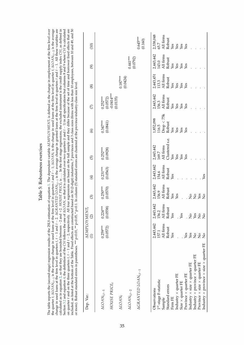
Tabl

e5:

Rob

ustn

ess

exer

cise

s

The

tabl

ere

port

sth

e(s

econ

d-st

age)

regr

essi

onre

sult

sof

the

2SLS

esti

mat

ion

ofeq

uati

on1.

The

depe

nden

tvar

iabl

e∆

EM

PLO

YM

EN

T tis

defin

edas

the

chan

gein

empl

oym

enta

tthe

firm

leve

love

rth

equ

arte

rt;

∆LO

AN

t,t−

1is

the

aver

age

chan

gein

used

loan

sat

the

firm

leve

lin

quar

ters

tan

dt−

1;∆

LOA

Nt

isth

ech

ange

inus

edlo

ans

atth

efir

mle

veli

nqu

arte

rt;

∆LO

AN

t,t−

2is

the

aver

age

chan

gein

used

loan

sat

the

firm

leve

lin

quar

ters

t,t−

1an

dt−

2.∆

GR

AN

TE

DLO

AN

t,t−

1is

the

aver

age

chan

gein

gran

ted

loan

sat

the

firm

leve

lin

quar

ters

tan

dt−

1.A

llth

ese

vari

able

sar

eca

lcul

ated

asin

equa

tion

2,so

that

they

are

boun

ded

betw

een−

2an

d+

2.H

OU

SEP

RIC

E tis

....

Inth

efir

stst

age

regr

essi

ons,

the

excl

uded

inst

rum

enti

sth

ecr

edit

supp

lyin

dex

CS

I,as

defin

edin

Sect

ion

3.2

and

equa

tion

4;th

ede

finit

ion

ofth

eC

SI

follo

ws

the

one

of∆

LOA

N,s

oth

atit

isca

lcul

ated

over

two

quar

ters

(tan

dt−

1)in

alls

peci

ficat

ions

butc

olum

ns8

and

9w

here

CS

Iis

calc

ulat

edon

quar

ter

tan

don

the

thre

equ

arte

rst,

t−1

and

t−2,

resp

ecti

vely

.A

llfo

urre

gres

sion

sar

eba

sed

onth

efu

llsa

mpl

ean

dth

eydi

ffer

beca

use

ofth

ese

tof

tim

ean

dbo

rrow

erfix

edef

fect

sth

atar

ein

clud

ed,a

slis

ted

atth

ebo

ttom

ofth

eTa

ble.

Fixe

def

fect

sar

eco

nstr

ucte

dba

sed

on30

(2-d

igit

)ind

ustr

ies,

7pr

ovin

ces

and

3cl

ass

size

s(fi

rms

wit

hle

ssth

an10

empl

oyee

s,be

twee

n10

and

49,a

nd50

orm

ore)

.Rob

usts

tand

ard

erro

rsin

pare

nthe

ses.

***

p<0.

01,*

*p<

0.05

,*p<

0.1.

Inco

lum

n(5

)sta

ndar

der

rors

are

clus

tere

dat

the

prov

ince

-ind

ustr

y-cl

ass

size

leve

l.

Dep

.Var

.:∆

EM

PLO

YM

EN

T t(1

)(2

)(3

)(4

)(5

)(6

)(7

)(8

)(9

)(1

0)

∆LO

AN

t,t−

10.

259*

**0.

224*

**0.

250*

**0.

231*

**0.

252*

**0.

347*

**0.

252*

**(0

.057

2)(0

.055

8)(0

.057

0)(0

.056

3)(0

.092

8)(0

.084

1)(0

.057

2)H

OU

SEP

RIC

E t-0

.041

4***

(0.0

135)

∆LO

AN

t0.

187*

**(0

.042

4)∆

LOA

Nt,t−

20.

441*

**(0

.079

2)∆

GR

AN

TE

DLO

AN

t,t−

10.

645*

**(0

.160

)

Obs

erva

tion

s2,

443,

442

2,44

3,44

22,

443,

442

2,44

3,44

22,

443,

442

1,85

2,09

82,

443,

442

2,44

3,45

12,

443,

442

2,33

8,04

81st

-sta

geF-

stat

isti

c15

7.1

156.

215

6.9

154.

616

9.7

116.

515

6.3

113.

314

3.0

65.7

Sam

ple

All

firm

sA

llfir

ms

All

firm

sA

llfir

ms

All

firm

sD

rop<

75k

All

firm

sA

llfir

ms

All

firm

sA

llfir

ms

Stan

dard

erro

rsR

obus

tR

obus

tR

obus

tR

obus

tC

lust

ered

s.e.

Rob

ust

Rob

ust

Rob

ust

Rob

ust

Rob

ust

Firm

FEYe

sYe

sYe

sYe

sYe

sYe

sYe

sYe

sYe

sYe

sIn

dust

ry×

quar

ter

FE.

.Ye

s.

Yes

Yes

Yes

Yes

Yes

Yes

Size

×qu

arte

rFE

.Ye

s.

.Ye

sYe

sYe

sYe

sYe

sYe

sPr

ovin

ce×

quar

ter

FEYe

s.

..

Yes

Yes

Yes

Yes

Yes

Yes

Indu

stry

×si

ze×

quar

ter

FEYe

sN

oN

o.

..

..

..

Indu

stry

×pr

ovin

ce×

quar

ter

FEN

oYe

sN

o.

..

..

..

Prov

ince

×si

ze×

quar

ter

FEN

oN

oYe

s.

..

..

..

Indu

stry

×pr

ovin

ce×

size

×qu

arte

rFE

No

No

No

Yes

..

..

..

35

Table 6: Job contract heterogeneity

The table reports the (second-stage) regression results of the 2SLS estimation of equation 1. The dependent variable∆EMPLOYMENTt is defined as the change in employment at the firm level over the quarter t, for the different types of jobcontracts, as labeled in each column, divided by the average stock of all firm’s workers over the quarter. Thus, the dependentvariable is not a growth rate but a contribution to the aggregate (at the firm level) growth rate. This means that the estimatedcoefficients cannot be interpreted as elasticities, but they need to be scaled by the relative share of the job contracts (see Table1). ∆LOANt,t−1 is the average change in used loans at the firm level in quarters t and t − 1. In the first stage regressions, theexcluded instrument is the credit supply index CSI, as defined in Section 3.2 and equation 4. The top panel reports the resultsfor two sub-samples of open-ended and temporary contracts, and the three sub-samples of contract termination (outflows) dueto dismissal, expiration of the contract, or voluntary quit. Temporary contracts includes fixed term direct hires, project workers,temporary agency workers, trainees and apprentices, and seasonal workers. The bottom panel reports the results for the sub-samples of changes in employment due to inflows or outflows, and the ones based on three different transitions: from temporaryto open-ended contracts, from full-time to part-time jobs, and from part-time to full-time jobs. All regressions are based on thefull sample and include the same set of time and borrower fixed effects, as listed at the bottom of the Table. Fixed effects areconstructed based on 30 (2-digit) industries, 7 provinces and 3 class sizes (firms with less than 10 employees, between 10 and 49,and 50 or more). Robust standard errors in parentheses. *** p<0.01, ** p<0.05, * p<0.1.

Dep. Var.: ∆EMPLOYMENTt

Contracts Reason of exitOpen-ended Temporary Dismissal Expiry Quit

∆LOANt,t−1 0.0652** 0.1850*** -0.0272 -0.124*** -0.0116(0.0314) (0.0471) (0.0222) (0.0300) (0.0275)

Flows TransitionsInflows Outflows Fixed to open Full to part-time Part-time to full

∆LOANt,t−1 0.0690 -0.179*** 0.0210** -0.00263 -0.00429(0.0447) (0.0508) (0.00867) (0.00654) (0.00594)

Observations 2,443,442 2,443,442 2,443,442 2,443,442 2,443,4421st-stage F-statistic 156.3 156.3 156.3 156.3 156.3Firm FE Yes Yes Yes Yes YesIndustry × quarter FE Yes Yes Yes Yes YesSize × quarter FE Yes Yes Yes Yes YesProvince × quarter FE Yes Yes Yes Yes Yes

36

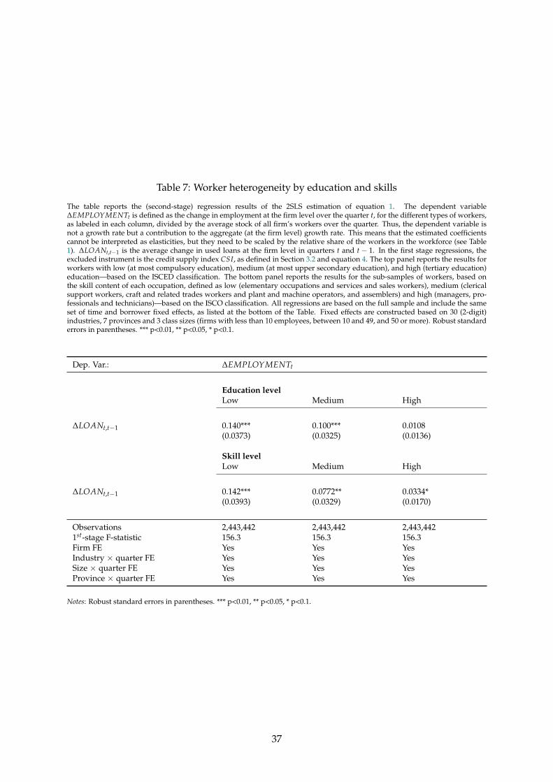
Table 7: Worker heterogeneity by education and skills

The table reports the (second-stage) regression results of the 2SLS estimation of equation 1. The dependent variable∆EMPLOYMENTt is defined as the change in employment at the firm level over the quarter t, for the different types of workers,as labeled in each column, divided by the average stock of all firm’s workers over the quarter. Thus, the dependent variable isnot a growth rate but a contribution to the aggregate (at the firm level) growth rate. This means that the estimated coefficientscannot be interpreted as elasticities, but they need to be scaled by the relative share of the workers in the workforce (see Table1). ∆LOANt,t−1 is the average change in used loans at the firm level in quarters t and t − 1. In the first stage regressions, theexcluded instrument is the credit supply index CSI, as defined in Section 3.2 and equation 4. The top panel reports the results forworkers with low (at most compulsory education), medium (at most upper secondary education), and high (tertiary education)education—based on the ISCED classification. The bottom panel reports the results for the sub-samples of workers, based onthe skill content of each occupation, defined as low (elementary occupations and services and sales workers), medium (clericalsupport workers, craft and related trades workers and plant and machine operators, and assemblers) and high (managers, pro-fessionals and technicians)—based on the ISCO classification. All regressions are based on the full sample and include the sameset of time and borrower fixed effects, as listed at the bottom of the Table. Fixed effects are constructed based on 30 (2-digit)industries, 7 provinces and 3 class sizes (firms with less than 10 employees, between 10 and 49, and 50 or more). Robust standarderrors in parentheses. *** p<0.01, ** p<0.05, * p<0.1.

Dep. Var.: ∆EMPLOYMENTt

Education levelLow Medium High

∆LOANt,t−1 0.140*** 0.100*** 0.0108(0.0373) (0.0325) (0.0136)

Skill levelLow Medium High

∆LOANt,t−1 0.142*** 0.0772** 0.0334*(0.0393) (0.0329) (0.0170)

Observations 2,443,442 2,443,442 2,443,4421st-stage F-statistic 156.3 156.3 156.3Firm FE Yes Yes YesIndustry × quarter FE Yes Yes YesSize × quarter FE Yes Yes YesProvince × quarter FE Yes Yes Yes

Notes: Robust standard errors in parentheses. *** p<0.01, ** p<0.05, * p<0.1.

37

Table 8: Worker heterogeneity by personal characteristics

The table reports the (second-stage) regression results of the 2SLS estimation of equation 1. The dependent variable∆EMPLOYMENTt is defined as the change in employment at the firm level over the quarter t, for the different types of workers,as labeled in each column, divided by the average stock of all firm’s workers over the quarter. Thus, the dependent variable isnot a growth rate but a contribution to the aggregate (at the firm level) growth rate. This means that the estimated coefficientscannot be interpreted as elasticities, but they need to be scaled by the relative share of the workers in the workforce (see Table1). ∆LOANt,t−1 is the average change in used loans at the firm level in quarters t and t − 1. In the first stage regressions, theexcluded instrument is the credit supply index CSI, as defined in Section 3.2 and equation 4. The left panel reports the results forthe sub-samples of men and women. The middle panel reports the results for the sub-samples of workers whose age is below orabove 30 years. The right panel show the results for the sub-sample of Italian and foreign workers. All regressions are based onthe full sample and include the same set of time and borrower fixed effects, as listed at the bottom of the Table. Fixed effects areconstructed based on 30 (2-digit) industries, 7 provinces and 3 class sizes (firms with less than 10 employees, between 10 and 49,and 50 or more). Robust standard errors in parentheses. *** p<0.01, ** p<0.05, * p<0.1.

Dep. Var.: ∆EMPLOYMENTt

Gender Age NationalityMale Female under 30 Over 30 Italian Foreign

∆LOANt,t−1 0.0741** 0.178*** 0.0867*** 0.164*** 0.172*** 0.0788***(0.0360) (0.0386) (0.0287) (0.0441) (0.0474) (0.0243)

Observations 2,443,442 2,443,442 2,443,442 2,443,442 2,443,442 2,443,4421st-stage F-statistic 156.3 156.3 156.3 156.3 156.3 156.3Firm FE Yes Yes Yes Yes Yes YesIndustry × quarter FE Yes Yes Yes Yes Yes YesSize × quarter FE Yes Yes Yes Yes Yes YesProvince × quarter FE Yes Yes Yes Yes Yes Yes

Notes: Robust standard errors in parentheses. *** p<0.01, ** p<0.05, * p<0.1.

38

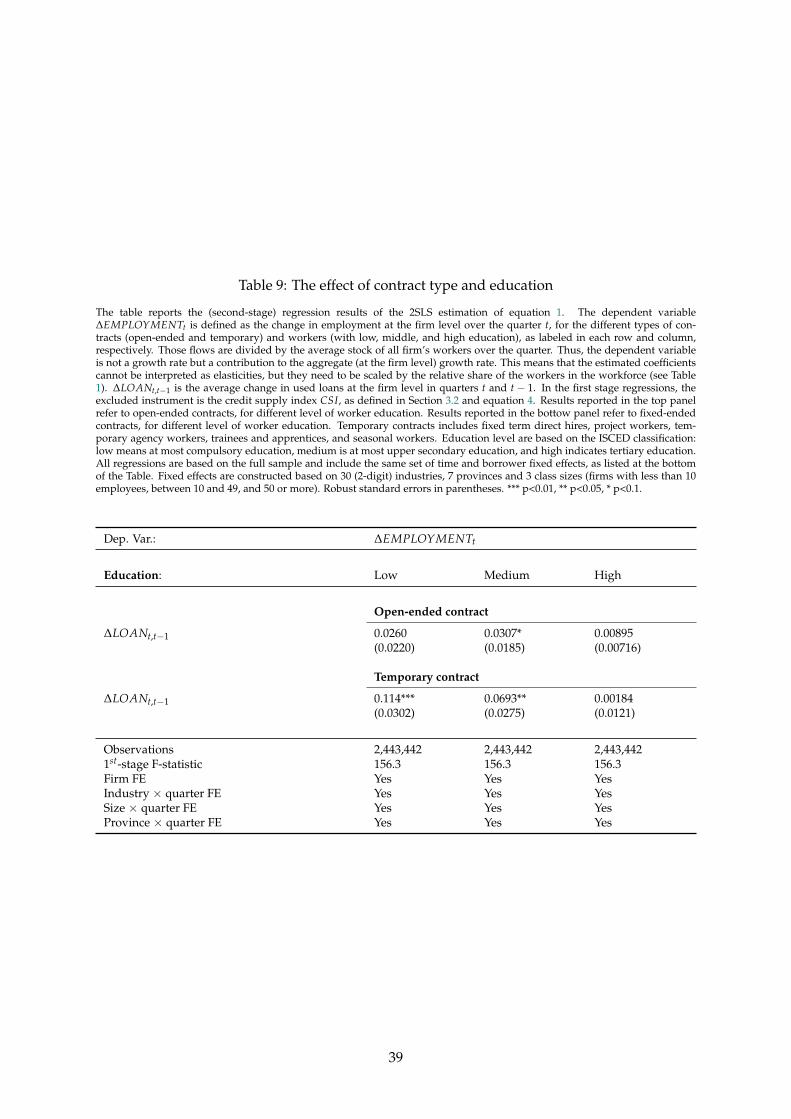
Table 9: The effect of contract type and education

The table reports the (second-stage) regression results of the 2SLS estimation of equation 1. The dependent variable∆EMPLOYMENTt is defined as the change in employment at the firm level over the quarter t, for the different types of con-tracts (open-ended and temporary) and workers (with low, middle, and high education), as labeled in each row and column,respectively. Those flows are divided by the average stock of all firm’s workers over the quarter. Thus, the dependent variableis not a growth rate but a contribution to the aggregate (at the firm level) growth rate. This means that the estimated coefficientscannot be interpreted as elasticities, but they need to be scaled by the relative share of the workers in the workforce (see Table1). ∆LOANt,t−1 is the average change in used loans at the firm level in quarters t and t − 1. In the first stage regressions, theexcluded instrument is the credit supply index CSI, as defined in Section 3.2 and equation 4. Results reported in the top panelrefer to open-ended contracts, for different level of worker education. Results reported in the bottow panel refer to fixed-endedcontracts, for different level of worker education. Temporary contracts includes fixed term direct hires, project workers, tem-porary agency workers, trainees and apprentices, and seasonal workers. Education level are based on the ISCED classification:low means at most compulsory education, medium is at most upper secondary education, and high indicates tertiary education.All regressions are based on the full sample and include the same set of time and borrower fixed effects, as listed at the bottomof the Table. Fixed effects are constructed based on 30 (2-digit) industries, 7 provinces and 3 class sizes (firms with less than 10employees, between 10 and 49, and 50 or more). Robust standard errors in parentheses. *** p<0.01, ** p<0.05, * p<0.1.

Dep. Var.: ∆EMPLOYMENTt

Education: Low Medium High

Open-ended contract

∆LOANt,t−1 0.0260 0.0307* 0.00895(0.0220) (0.0185) (0.00716)

Temporary contract

∆LOANt,t−1 0.114*** 0.0693** 0.00184(0.0302) (0.0275) (0.0121)

Observations 2,443,442 2,443,442 2,443,4421st-stage F-statistic 156.3 156.3 156.3Firm FE Yes Yes YesIndustry × quarter FE Yes Yes YesSize × quarter FE Yes Yes YesProvince × quarter FE Yes Yes Yes

39

Table 10: Firm heterogeneity by size and sector

The table reports the (second-stage) regression results of the 2SLS estimation of equation 1. The dependent variable∆EMPLOYMENTt is defined as the change in employment at the firm level over the quarter t; ∆LOANt,t−1 is the averagechange in used loans at the firm level in quarters t and t − 1. In the first stage regressions, the excluded instrument is the creditsupply index CSI, as defined in Section 3.2 and equation 4. The left panel reports the results for three sub-samples defined on thebasis of firm size. Firm size bins identify micro (less than 10 employees), small (between 10 and 49 employees) and medium andlarge firms (50 or more employees). The right panel reports the results for the sub-sample of firms in the industry and servicesectors. All regressions are based on the full sample and include the same set of time and borrower fixed effects, as listed at thebottom of the Table. Fixed effects are constructed based on 30 (2-digit) industries, 7 provinces and 3 class sizes (firms with lessthan 10 employees, between 10 and 49, and 50 or more). Robust standard errors in parentheses. *** p<0.01, ** p<0.05, * p<0.1.

Dep. Var.: ∆EMPLOYMENTt

Firm size SectorMicro Small Med-Large Industry Services

∆LOANt,t−1 0.246*** 0.306** 3.449 0.0888 0.304***(0.0609) (0.158) (16.523) (0.106) (0.0680)

Observations 2,072,535 332,163 38,744 811,391 1,632,0511st-stage F-statistic 131.9 27.73 0.206 35.97 121.0Firm FE Yes Yes Yes Yes YesIndustry × quarter FE Yes Yes Yes Yes YesSize × quarter FE Yes Yes Yes Yes YesProvince × quarter FE Yes Yes Yes Yes Yes

Table 11: Firm heterogeneity by financial characteristics

The table reports the (second-stage) regression results of the 2SLS estimation of equation 1. The dependent variable∆EMPLOYMENTt is defined as the change in employment at the firm level over the quarter t; ∆LOANt,t−1 is the averagechange in used loans at the firm level in quarters t and t − 1. In the first stage regressions, the excluded instrument is the creditsupply index CSI, as defined in Section 3.2 and equation 4. The left panel reports the results for the sub-samples of firms withlow and high debt per employee at the beginning of the period (the split is done around the median comparing firms in the samesector and size class). The middle panel reports the results for the sub-samples of firms which at the beginning of the periodhad a low and high utilization of granted credit lines (i.e. with the ratio of utilized loans over granted loans below or abovethe median). The right panel separates between firms which borrows from only one bank (Single-bank) and firms with multiplebanking relationships (Multi-banks). All regressions are based on the full sample and include the same set of time and borrowerfixed effects, as listed at the bottom of the Table. Fixed effects are constructed based on 30 (2-digit) industries, 7 provinces and3 class sizes (firms with less than 10 employees, between 10 and 49, and 50 or more). Robust standard errors in parentheses. ***p<0.01, ** p<0.05, * p<0.1.

Dep. Var.: ∆EMPLOYMENTt

Debt Credit lines use Relationship lendingLow High Low High Single-bank Multi-banks

∆LOANt,t−1 0.183*** 0.358*** 0.206*** 0.315*** 0.303*** 0.397***(0.056) (0.123) (0.064) (0.107) (0.098) (0.201)

Observations 1,199,222 1,244,220 1,214,350 1,229,092 1,384,664 1,006,5911st-stage F-statistic 101.8 79.3 89.3 72.5 60.7 23.5Firm FE Yes Yes Yes Yes Yes YesIndustry × quarter FE Yes Yes Yes Yes Yes YesSize × quarter FE Yes Yes Yes Yes Yes YesProvince × quarter FE Yes Yes Yes Yes Yes Yes

Notes: Robust standard errors in parentheses. *** p<0.01, ** p<0.05, * p<0.1.

40

Online Appendix

A-I Additional Tables

Table A1: The effect of contract type within firm sector and size

The table reports the (second-stage) regression results of the 2SLS estimation of equation 1. The dependent variable∆EMPLOYMENTt is defined as the change in employment at the firm level over the quarter t, for the different types of jobcontracts—open-ended in the top panel and temporary contract in the bottom panel—divided by the average stock of all firm’sworkers over the quarter. Temporary contracts includes fixed term direct hires, project workers, temporary agency workers,trainees and apprentices, and seasonal workers. Thus, the dependent variable is not a growth rate but a contribution to the ag-gregate (at the firm level) growth rate. This means that the estimated coefficients cannot be interpreted as elasticities, but theyneed to be scaled by the relative share of the job contracts (see Table 1). Results are reported for different sub-samples acrosssectors (industry and services) and firm size. Firm size bins identify micro (less than 10 employees), small (between 10 and 49employees) and medium and large firms (50 or more employees). ∆LOANt,t−1 is the average change in used loans at the firmlevel in quarters t and t − 1. In the first stage regressions, the excluded instrument is the credit supply index CSI, as definedin Section 3.2 and equation 4. All regressions are based on the full sample and include the same set of time and borrower fixedeffects, as listed at the bottom of the Table. Fixed effects are constructed based on 30 (2-digit) industries, 7 provinces and 3 classsizes (firms with less than 10 employees, between 10 and 49, and 50 or more). Robust standard errors in parentheses. *** p<0.01,** p<0.05, * p<0.1.

Dep. Var.: ∆EMPLOYMENTt

Over sectors Over firm size

Open-ended contract

∆LOANt,t−1 0.0550 0.0660** 0.0573* 0.109 0.817(0.0756) (0.0327) (0.0333) (0.0907) (2.276)

Temporary contract

∆LOANt,t−1 0.0356 0.235*** 0.186*** 0.192 1.462(0.0757) (0.0585) (0.0507) (0.122) (3.975)

Observations 811,391 1,632,051 2,072,535 330,973 39,9341st-stage F-statistic 35.97 121.0 131.9 27.73 0.206Sector Industry Services All firms All firms All firmsFirm size All firms All firms Micro Small Medium-largeFirm FE Yes Yes Yes Yes YesIndustry × quarter FE Yes Yes Yes Yes YesSize × quarter FE Yes Yes Yes Yes YesProvince × quarter FE Yes Yes Yes Yes Yes

41

Table A2: The effect of education within firm sector and size

The table reports the (second-stage) regression results of the 2SLS estimation of equation 1. The dependent variable∆EMPLOYMENTt is defined as the change in employment at the firm level over the quarter t, for the different levels ofeducation—low, medium and high—divided by the average stock of all firm’s workers over the quarter. Temporary contractsincludes fixed term direct hires, project workers, temporary agency workers, trainees and apprentices, and seasonal workers.Education level are based on the ISCED classification: low means at most compulsory education, medium is at most upper sec-ondary education, and high indicates tertiary education. Thus, the dependent variable is not a growth rate but a contributionto the aggregate (at the firm level) growth rate. This means that the estimated coefficients cannot be interpreted as elasticities,but they need to be scaled by the relative share of the job contracts (see Table 1). Results are reported for different sub-samplesacross sectors (industry and services) and firm size. Firm size bins identify micro (less than 10 employees), small (between 10and 49 employees) and medium and large firms (50 or more employees). ∆LOANt,t−1 is the average change in used loans at thefirm level in quarters t and t − 1. In the first stage regressions, the excluded instrument is the credit supply index CSI, as definedin Section 3.2 and equation 4. All regressions are based on the full sample and include the same set of time and borrower fixedeffects, as listed at the bottom of the Table. Fixed effects are constructed based on 30 (2-digit) industries, 7 provinces and 3 classsizes (firms with less than 10 employees, between 10 and 49, and 50 or more). Robust standard errors in parentheses. *** p<0.01,** p<0.05, * p<0.1.

Dep. Var.: ∆EMPLOYMENTt

Over sectors Over firm size

Low education

∆LOANt,t−1 0.0671 0.165*** 0.131*** 0.199* 1.755(0.0805) (0.0415) (0.0397) (0.105) (4.685)

Medium education

∆LOANt,t−1 0.0192 0.127*** 0.103*** 0.0885 0.390(0.0545) (0.0398) (0.0355) (0.0718) (1.156)

High education

∆LOANt,t−1 -0.00179 0.0142 0.0115 0.0112 0.0595(0.0190) (0.0173) (0.0149) (0.0288) (0.306)

Observations 811,391 1,632,051 2,072,535 330,973 39,9341st-stage F-statistic 35.97 121.0 131.9 27.73 0.206Sector Industry Services All firms All firms All firmsFirm size All firms All firms Micro Small Medium-largeFirm FE Yes Yes Yes Yes YesIndustry × quarter FE Yes Yes Yes Yes YesSize × quarter FE Yes Yes Yes Yes YesProvince × quarter FE Yes Yes Yes Yes Yes

42

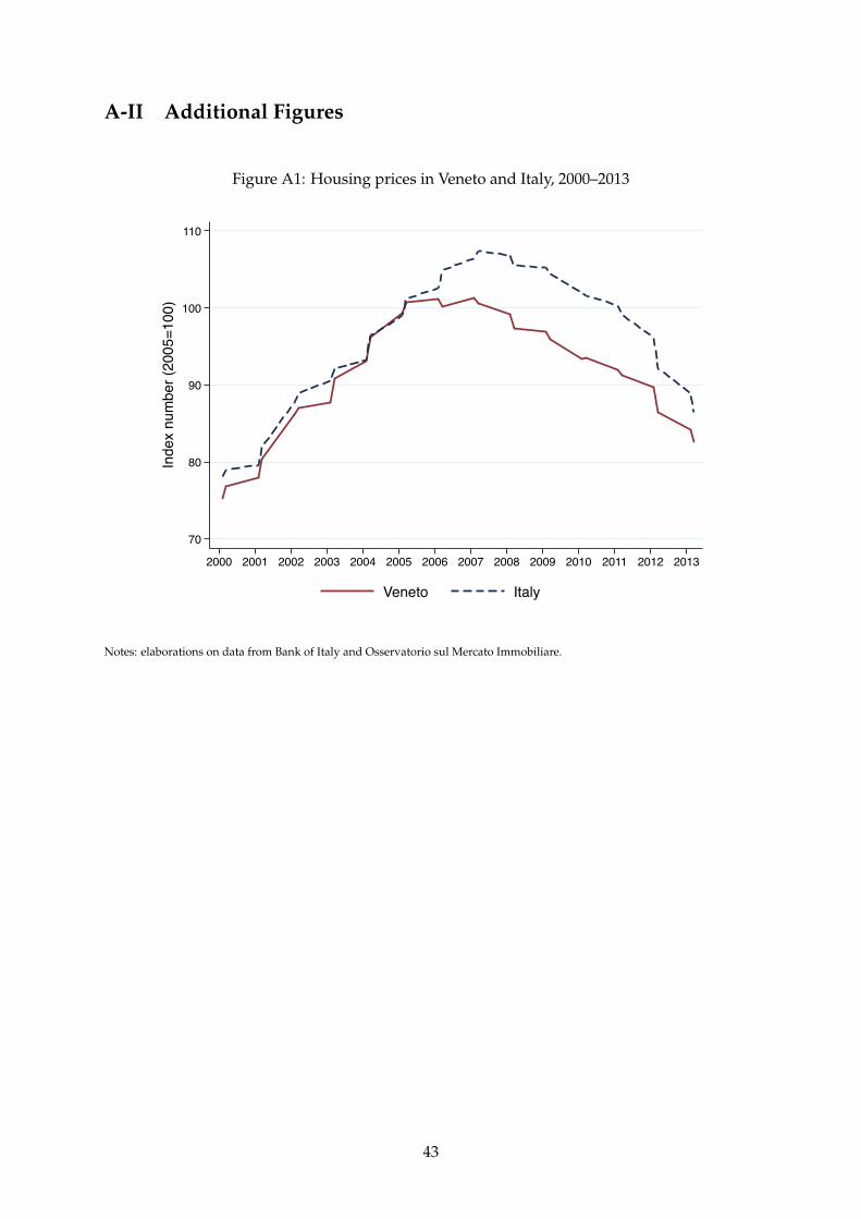
A-II Additional Figures

Figure A1: Housing prices in Veneto and Italy, 2000–2013

70

80

90

100

110

Inde

x nu

mbe

r (20

05=1

00)

2000 2001 2002 2003 2004 2005 2006 2007 2008 2009 2010 2011 2012 2013

Veneto Italy

Notes: elaborations on data from Bank of Italy and Osservatorio sul Mercato Immobiliare.

43