banking and currency crises: differential diagnostics for

Working Paper Series

Banking and currency crises: differential diagnostics for developed countries

Mark Joy, Marek Rusnák, Kateřina Šmídková and Bořek Vašíček

No 1810 / June 2015

Note: This Working Paper should not be reported as representing the views of the European Central Bank (ECB). The views expressed are those of the authors and do not necessarily reflect those of the ECB

Abstract We identify a set of “rules of thumb” that characterise economic, financial and structural conditions preceding the onset of banking and currency crises in 36 advanced economies over 1970–2010. We use the Classification and Regression Tree methodology (CART) and its Random Forest (RF) extension, which permits the detection of key variables driving binary crisis outcomes, allows for interactions among key variables and determines critical tipping points. We distinguish between basic country conditions, country structural characteristics and international developments. We find that crises are more varied than they are similar. For banking crises we find that low net interest rate spreads in the banking sector and a shallow or inverted yield curve are their most important forerunners in the short term, whereas in the longer term it is high house price inflation. For currency crises, high domestic short-term rates coupled with overvalued exchange rates are the most powerful short-term predictors. We find that both country structural characteristics and international developments are relevant banking crisis predictors. Currency crises, however, seem to be driven more by country idiosyncratic, short-term developments. We find that some variables, such as the domestic credit gap, provide important unconditional signals, but it is difficult to use them as conditional signals and, more importantly, to find relevant threshold values.

JEL Codes: C14, E44, F37, F47, G01.

Keywords: Banking crises, binary classification tree, currency crises, early warning indicators.

ECB Working Paper 1810, June 2015 1

Nontechnical Summary

The recent global financial crisis has reinvigorated interest in models capable of identifying the warning signs of crisis. Early warning models are typically based on empirical logistic regressions. However, common regression-based models are unable to capture important non-linearities and complex interactions between macroeconomic and financial variables that may exist in the run-up to crises.

To address these issues we use Classification and Regression Tree (CART) methodology and its generalisation, Random Forest (RF) analysis, to model explicitly the non-linear interactions between variables and deal with missing values and outliers, which are usually a problem for regression-based frameworks. The CART and RF frameworks provide crisis thresholds for key variables, thus significantly simplifying the interpretation of the results for decision-makers and non-technical audiences.

This framework has both advantages and disadvantages compared with other common early warning methods. On the one hand, it allows explicitly for the fact that not all crises are alike and accommodates non-linearities by including conditional thresholds. On the other hand, it is a non-parametric approach that cannot estimate the marginal contributions of each explanatory variable or confidence intervals for the estimated thresholds.

We apply the CART and RF techniques on an unbalanced panel dataset consisting of 36 advanced countries between 1970 and 2010. We investigate what macroeconomic, financial and structural conditions prevailed in the economies in the periods ahead of banking and currency crises in this period.

Our results suggest that one-to-two years ahead of a banking crisis the net interest rate spread in the banking sector is the key predictor of crisis. The crises are more likely to occur when this spread is low. On the contrary, if net interest rate spreads in the banking sector are high, then a flat or inverted yield curve becomes the crucial predictor of banking crisis. We interpret this as evidence that the term spread can be thought of as representing the marginal profitability of bank lending, and compression of the term spread, if occurring at the peak of a banking boom, can be a causal signal of bust. Two-to-three years ahead of a banking crisis, house prices seem to be the most important predictor of crisis onset. As for currency crises, the most powerful predictor one-to-two years ahead is exchange rate overvaluation combined with high domestic short-term interest rates.

We also evaluate the importance of country-specific structural factors and international variables in predicting crises. For banking crises, we find that both country structural characteristics and international developments are relevant crisis predictors. Currency crises, however, seem to be driven mainly by country-specific short-term developments.

It should be noted that our results, like the results of any early warning model, are conditioned on the country sample, time span and predictors. As such, the results should be considered mainly as a structured presentation of past experience and should not, without due care, be used for predicting future crises.


1. Introduction

Until recently most of the empirical research on predictors or determinants of financial crises has focused on emerging market economies. The US subprime crisis and the euro area debt crisis have awakened interest in systemic approaches to the early identification of crises in advanced countries. Compared with emerging market economies, which are often characterised by economic and financial market volatility in the run-up to crises, the pre-crisis conditions in advanced countries are often much smoother, making the identification of robust early warning signals more challenging. This is further complicated by the fact that there is substantial disagreement over the dating of crisis periods – Babecký et al. (2014) find this for advanced economies while Arteta and Eichengreen (2000) show that for emerging market economies dating banking crises can be just as problematic. On the other hand, advanced countries are arguably more homogeneous than emerging market economies in terms of their economic characteristics, which may improve the reliability of crisis signals. Yet, higher homogeneity does not imply necessarily that all advanced country crises will be alike. This represents additional challenges for the early warning literature given that it aims to identify common drivers of different periods of economic and financial turmoil. Indeed, regression-based early warning models are based on the strong assumption that the marginal contribution of each indicator to the probability of crisis does not depend on the value of the indicator for all countries over all time periods.

The purpose of this paper is to identify a set of economic “rules of thumb” that characterise economic, financial and structural conditions preceding the onset of financial crises in 36 advanced countries (EU countries and non-EU OECD countries) between 1970 and 2010. We use a quarterly database of crises in advanced countries constructed by Babecký et al. (2012), investigating banking and currency crises separately.1 We use the Classification and Regression Tree methodology (CART) advanced by Breiman et al. (1984), specifically the Binary Classification Tree (BCT) approach, which permits the detection of key variables driving crises, allows for interaction effects and determines critical tipping points.2 This framework has both advantages and disadvantages compared with other common early warning methods, namely the discrete choice models (logits or probits). On the one hand, it allows explicitly for the fact that not all crises are alike and accommodates non-linearities by including variables’ conditional thresholds. This advantage should not be understated. Unlike logit models, which do not provide policymakers with easily actionable advice on when to act to prevent a crisis (marginal effects provide a continuum of easily ignorable probabilities rather than a yes-no recommendation on action), CART is able to tell the policymaker that while some crisis indicators may be indicative of the average propensity for crisis, the specific conditions of the policymaker’s country are important, and under these specific conditions, certain crisis indicators are more reliable than others, and CART can highlight which indicators these are. CART helps us to identify, for instance, that while rapid house price inflation is a good predictor of banking crises 2–3 years ahead, banking crises can also be consistent with sluggish house price growth, if short-term interest rates are low and the yield curve flat (almost half the banking crises in our sample can be identified as having these characteristics). On the other hand, CART is a non-parametric approach

1 We note that sovereign debt crises have been less common in advanced countries than emerging market economies, with the incidence so rare that we exclude them from our empirical analysis on the basis that any inference drawn would be statistically fragile. 2 Binary trees have the property that only two branches can depart from the same node.


so cannot calculate the marginal contributions of each explanatory variable or confidence intervals for the estimated thresholds. While typical early warning analyses look for indicators that are unconditional triggers of crises, in the logic of the CART approach an indicator can become a trigger only when it breaches a certain threshold or when it interacts with another indicator. This makes the comparability of CART with traditional regression approaches complicated, although they can be complements in the policymaker’s toolkit. In addition, we use the Random Forest (RF) algorithm, which is an extension of CART, to overcome some of the weaknesses of the CART approach.

Our contributions are as follows: (i) we look at advanced countries given that advanced countries were at the epicentre of the global financial crises, whereas most studies centre their analysis on emerging market economies, which are arguably substantially more heterogeneous with more dispersed economic developments; this might be problematic especially when one wants to identify a common threshold across countries; (ii) we use a quarterly dataset, which allows us to provide more detailed crisis-dating information, especially when it comes to distinguishing between crisis onset and crisis occurrence; (iii) we extend the common list of leading indicators beyond domestic macro-financial variables (i.e. the core indicators providing “differential diagnostics”) by including (1) domestic factors that have significant cross-country variation but vary significantly less over time and can, as such, be seen as structural characteristics of the economy (e.g. economic openness, exchange rate regime or financial development) so as to further deal with country heterogeneity in a more explicit way than the common fixed-effects approach, and (2) international factors that can, in addition to having a direct effect on the domestic economy, contribute to crises indirectly by interacting with domestic variables (e.g. commodity prices, global GDP growth and global private credit);3 and finally (iv) we focus on both banking crises and currency crises, and by doing so, we get an insight into common determinants.

It should be noted that our results, like the results of any early warning model, are conditioned on the country sample, time span and predictors. We do not claim to identify causality. Our results should be considered mainly as a structured presentation of past experience and should not, without due care, be used for predicting future crises.

Our results feature a number of interesting findings: (i) we find that a high net interest rate spread in the banking sector (i.e. the spread between the loan and deposit rate) combined with a flat or inverted yield curve are the most reliable indicators of banking crises one-to-two years ahead of a crisis; we interpret this as evidence in favour of the hypothesis put forward by Adrian et al. (2010) that the term spread can be thought of as representing the marginal profitability of bank lending, and compression of the term spread, at the peak of a banking boom, can be a causal signal of bust; (ii) house prices are the key predictor of banking crises further ahead (in two to three years’ time), supporting the idea that different indicators have predictive power at different horizons (e.g. Bussiere, 2013b); (iii) for currency crises, very high short-term interest rates coupled with an overvalued exchange rate (i.e. significantly above its trend value) are common predictors; (iv) some observable domestic structural characteristics such as trade openness, economic structure and financial development substantially affect the propensity for banking crises, whereas other 3 On the other hand, in our empirical setting it is very difficult to deal with contagion explicitly. Contagion has been considered in the early warning literature (e.g. in Bussiere, 2013b) by means of cross-country correlations of equity markets.


structural characteristics, such as the exchange rate regime, are not found to be relevant; (v) international variables, in particular world GDP, interact significantly with country variables in the prediction of banking crises; (vi) for currency crises, predictors are largely idiosyncratic to the country and of a short-term (rather than structural) nature.

The rest of the paper is organised as follows. Section 2 provides a selective survey of studies employing similar methodology. Section 3 describes the selection tree and random forest techniques. In Section 4 we detail our crisis database and the set of selected crisis forerunners. All the empirical results for both banking and currency crises are presented in Section 5. Section 6 provides robustness checks. Section 7 makes comparisons with the traditional regression-based framework and other studies. Section 8 concludes.

2. Selective Literature Survey

Most of the literature aiming to identify financial-crisis triggers focuses on early warning models with two different approaches. The first is the (non-parametric) univariate signalling approach (Kaminsky and Reinhart, 1999; Borio and Lowe, 2002; Borio and Drehmann, 2009), which looks at the behaviour of individual variables around crisis episodes and tries to extract signals defined in terms of specific thresholds. The second is the (parametric) multivariate approach, in particular the logit model (Demirgüç-Kunt and Detragiache, 1998; 2005; Bussiere and Fratzscher, 2006), but recently also more formal procedures such as Bayesian model averaging (Babecký et al., 2012a,b; Crespo Cuaresma and Slacik, 2009).

The multivariate CART methodology lies between these approaches, taking into account the predominantly discrete nature of crises but also providing more organised selection of crisis triggers. Similar to typical signalling approaches it allows for subjective selection of the trade-off between missed crises and false alarms (Type I vs. Type II errors). Unlike the previous regression-based methods it looks for non-linear and conditional relations between crisis triggers. Therefore, it allows not only for detection of the main crisis triggers and their threshold values, but also for a combination of conditions (rules) that typically increase the probability of a crisis.

A number of papers use CART to explore the triggers of sovereign debt crises (Manasse et al., 2003; Manasse and Roubini, 2009; Savona and Vezzoli, 2008, 2012), currency or balance-of-payment crises (Ghosh and Ghosh, 2002; Frankel and Wei, 2004; Chamon et al., 2007) and banking crises (Dattagupta and Cashin, 2011; Davis et al., 2011). All these papers look at emerging and developing economies and use annual data. Apart from Davis et al. (2011) they do not deal explicitly with regional heterogeneity. For sovereign debt crises, Manasse and Roubini (2009) find that the external debt-GDP ratio (a value above 50%) is the main trigger if it is accompanied by other imbalances such as high inflation (over 10%) or reliance on short maturity finance (short-term external debt to foreign exchange reserves above 1.3%). Another finding is that the in-sample fit is substantially better than the out-of-sample prediction, although this finding is not specific to CART but applies to most EW literatures. Savona and Vezzoli (2013) try to overcome this problem by a two-step procedure to improve the ratio between the fitting and forecasting ability of the model.

For banking crises, Dattagupta and Cashin (2011) study 50 emerging market economies (1990–2005) highlighting the importance of macroeconomic risk (high inflation), foreign currency risk


(depreciation when bank deposits are highly dollarised) and poor financial soundness (low bank profitability). Davis and Karim (2008a) use CART to study 105 countries (1979–2003) and try to predict the recent sub-prime crisis based on an assessment of banking crises prior to 2000. The model selects real domestic credit growth; in particular, countries that experienced a yearly contraction of more than 4% were twice as likely to experience a banking crisis. Davis et al. (2011) study 20 emerging market economies in Asia and Latin America, comparing the estimated results of logit and CART. They argue that the causes of crises can differ across regions. For Latin America they find that the degree of local currency depreciation is the main crisis trigger, along with high levels of financial intermediation (bank credit/GDP) or inflation, and that credit contractions can be a key trigger of banking crises. For Asian countries fiscal discipline (budget balance/GDP) and slow GDP growth seem to be key.

For currency crises, Ghosh and Ghosh (2003) point to a combination of bad institutions (high corruption) and weak fundamentals (current account/GDP, corporate debt, external sovereign debt). Chamon et al. (2007) look specifically at capital account crises (“sudden stops”) using a sample of 49 emerging market economies (1994–2003) and identify reserve cover (gross international reserves/short-term external debt + current account deficit) as the main crisis trigger coupled with high external debt.

Finally, for sovereign debt crises, Manasse and Roubini (2009) look at 47 emerging market economies (1970–2002) and detect three different crisis combinations: liquidity (high short-term external debt to foreign exchange reserves), solvency (high total external debt as a share of GDP in combination with high inflation or high external financing requirements) and macroeconomic risk (very negative GDP growth). Savona and Vezzoli (2012, 2013) employ data for 66 emerging market economies (1975–2002) and extend the CART methodology (in a two-step procedure) in order to balance in-sample and out-of-sample accuracy. They confirm the importance of liquidity and solvency risks alongside systemic risk (contagion). One notable problem with the CART methodology is its sensitivity to time and cross-section. Consequently, the triggers of crises in advanced countries can be strikingly different.

3. Method

We employ classification trees, as pioneered by Breiman et al. (1984), for our analytical work on the classification and prediction of banking and currency crises.4 Classification trees are machine-learning methods for constructing prediction models that offer a non-parametric framework for uncovering non-linear and interactive structures in the data. The data are partitioned recursively and within each partition a simple prediction model is fitted. As a result, the partitioning can be represented graphically as a decision tree. Classification trees are designed for dependent variables that take a finite number of unordered values. Here, the dependent variable takes one of two possible values: crisis or no crisis. Unlike regression analysis, classification trees allow for the possibility that different relationships may hold between predictors at different times and under different cross-sectional conditions.

4 Our core empirical estimations are conducted using proprietary classification-tree software developed by Salford Systems. Our random forest algorithm is implemented in the programming environment R.


3.1 Classification Trees

Classification trees partition data recursively. Each parent node (a node represents a data partition determined by an explanatory variable) is split into two child nodes such that each child node has outcome characteristics that are more homogeneous than the parent node (where the outcome characteristics refer, here, to crisis periods and no crisis periods). This splitting process is repeated for each child node, until reaching a terminal node, which represents a final partitioning of the data. Each terminal node has attached to it a simple prediction model that applies to that terminal node only. In short, the classification-tree approach searches through different possible splits for all explanatory variables and selects those splits that best separate crisis episodes from no-crisis episodes. For example, in partitioning data for the classification of banking crises, the classification-tree algorithm will assess, in order to provide an adequate predictive description of periods of crisis, whether the steepness of the government-bond yield curve tends to be above a critical threshold (split) in advance of crisis periods. Is, for instance, the steepness of the domestic sovereign yield curve greater than one percentage point? The algorithm will assess all possible splits and select the one that best separates crisis episodes from non-crisis episodes. Our results suggest, for instance, that one-to-two years ahead of a banking crisis the steepness of the yield curve is usually flatter than 1.3 percentage points.

The splitting criterion is the minimisation of a loss function based on a cost that rises when the actual split deviates from the perfect split (where the perfect split partitions all crisis episodes into one node and all non-crisis episodes into another). Let p(i|t) be the fraction of occurrences belonging to class i at node t. In a two-class problem, such as here, and omitting the reference to node t, the class distribution at any node can be written as (p0, p1), where p0 is the posterior probability of a non-crisis observation falling into node t, and p1 is the posterior probability of a crisis observation falling into node t. Measures for selecting the best split are based on the degree of impurity in the child nodes. The more skewed the distribution, the smaller the degree of impurity. A node with class distribution (0, 1), for instance, has zero impurity, while a node with class distribution (0.5, 0.5) has maximum impurity.

We employ the Gini criterion as a primary splitting rule, which corresponds to the following impurity (or loss) function i(t), which we seek to minimise:

igini (t) = ∑ p0(t)p1(t)

This impurity function reaches a minimum when the terminal nodes contain only one of the two classes of observations: crisis or no crisis. Classification-tree analysis also allows the researcher to weight differently the costs of misclassifying crisis and no-crisis observations. Imposing a higher cost on failing to predict crises will raise p1(t) and increase the frequency with which crises are predicted. Setting misclassification costs within classification trees affects which indicator variables are selected and influences the threshold values. With traditional early warning models this is not the case. As Manasse and Roubini (2009) note, while it is possible to set misclassification costs for probit models, the selection of indicator variables in the probit model will not be affected. The model specification will remain unchanged. In all the following classification-tree specifications we follow Manasse and Roubini (2009) by setting the cost of


missing a crisis to seven times the cost of missing a no-crisis episode. There is no explicit rationale for choosing a multiple of seven; it is an arbitrary choice meant to reflect the policymaker’s strong preference for false alarms over costly crises (see Alessi and Detken, 2013 for a more detailed discussion of the relevance of policy preferences for early warning systems).

The growing of the tree terminates when the reduction in the misclassification rate associated with further splitting is less than the change in the penalty levied on the addition of further terminal nodes. Termination does not imply that it is always possible to obtain entirely homogeneous final nodes. The best tree in terms of goodness of fit is obtained by minimising the misclassification rate while penalising larger trees with more nodes.

Classification trees provide importance ranking of variables. Ranking allows us to compare classification-tree results with results from linear regression methods such as Bayesian model averaging (Babecký et al., 2014). It also helps us overcome the classification-tree problem of masking, whereby if one variable is even slightly outperformed by another variable, the under-performing variable may never appear in the final tree.

3.2 Strengths and Limitations

Despite its statistical appeal and usefulness to the policymaker in identifying crisis thresholds, the classification-tree approach suffers from a number of shortcomings. First, since classification trees attach a single probability to all cases belonging to the same class, the marginal contribution of each variable to the probability of observing an episode of either crisis or no crisis cannot be determined. Yet, at each node the variation in the probability linked to breaching that particular threshold can be computed. Second, confidence intervals for threshold values cannot be determined since the approach assumes nothing about probability distributions. Third, masking, as described above, may cause one of two explanatory variables, both important but similar in their ability to identify a split, to be absent from the final tree. Fourth, the recursive partitioning procedure draws, with each step, less information from the full sample. Solutions therefore become increasingly localised and vulnerable to the criticism of being only one-step optimal rather than overall optimal (Breiman et al, 1984). This leads to the final weakness of classification trees: they can be prone to over-fitting if measures are not taken to avoid the problem (we discuss and incorporate such measures below).

The advantages of classification trees are many. (i) Interactions: Classification trees allow explicitly for interactions between explanatory variables, permitting the identification of heterogeneity across the sample space and non-linear relationships and threshold effects.5 (ii) Specification error. Classification trees are free from specification error since the method searches across the entire model space. (iii) Non-parametric: There is no requirement to pre-specify a functional form; classification trees can therefore cope with data that are highly skewed or multi-modal. (iv) Number of predictors: classification trees can deal with large numbers of predictor variables. (iv) Missing values: missing values are permitted. (v) Interpretability: Classification trees are simple to interpret. They provide feasible and practical rules of thumb for policymaking and crisis prevention.

5 Some of these issues can be dealt with in regression-based models as well, but this is substantially more complicated.


3.3 Random Forests

Despite its many strengths, the classification tree approach, if employed without due care, can produce results susceptible to over-fitting. That is, the approach can create overly complex trees that do not generalise well from the training data. We take a number of steps to avoid this.

First, rather than run the classification tree algorithm on the entire space of potential candidate variables, we run it on only those variables found to be most important by an implementation of the random forest algorithm (Breiman et al., 1984). Unlike the classification tree algorithm, which fits just a single tree to the data, a random forest fits many hundreds or thousands of trees (depending on the desired accuracy) from randomly permuted sub-samples of the data. Around two thirds of the data is selected in each sub-sample. The remaining data (called out-of-bag data) are preserved in order to establish variable importance and out-of-sample error rates. Each iteration issues a vote on variable importance and majority votes are used to yield the final, pooled, variable-importance rankings. Random forests offer two key advantages in this context: (i) insensitivity to outliers; and (ii) avoidance of over-fitting. Variable-importance rankings are, as a result, far more robust than those issued by a single classification tree.

The random forest algorithm can be summarised as follows (Liaw and Wiener, 2002):

1. Draw n bootstrap samples from the original data.

2. For each of the bootstrap samples, grow an unpruned classification tree, with the following modification: at each node, rather than choosing the best split among all predictors, randomly sample m of the predictors and choose the best split from among those variables.

3. Predict new data by aggregating the predictions of the n trees by majority votes.

A natural question to ask at this point is, if random forests offer such computational advantages, why do we use them only to establish measures of variable importance? Why do we not use them to also determine a decision tree of interactions and thresholds? The answer is straightforward: apart from what they can tell us about variable importance, random forests are difficult to interpret. By their very nature of being based on a majority-voting procedure from a multiplicity of sub-samples, they cannot be used to backward-induce a single tree of interaction effects. So once we have used random forests to inform us about variable importance, and select the most relevant variables, we return to the standard classification tree to shed light on interaction effects.

A second step we use to avoid over-fitting is pruning. After our random forest procedures have been run, and once we are in a position to construct a standard classification tree, avoidance of over-fitting is achieved by growing an overly large tree and then pruning its unreliable branches. Pruning can be regarded as a search problem, where one looks for the best pruned tree.

4. Dataset of Crises and Leading Indicators

There are two ways to select the horizons for crisis prediction in the early warning exercise. The common option is to set a fixed forward horizon for all potential predictors, such as precisely one


or two years ahead of a crisis. This approach addresses the question: “What could we expect to observe one or two years before a crisis breaks out?” This has an intuitive appeal in terms of early warning, but it comes at a cost of potentially missing important signals that might flash at different horizons between or outside these discrete dates. Therefore, an alternative way is to pre-select an optimal prediction horizon for each variable (Babecký et al., 2013), addressing the issue of “whether and when a particular variable can provide information about crises”. This approach is more suitable for crisis variables that take a continuous rather than discrete form. Its drawback is that it is rather less intuitive in practice. Indeed, it is more common to observe developments of diverse economic indicators at the time rather than assuming that indicator A is relevant for developments say within one year and indicator B for developments within three years.

Our goal is not to predict the exact timing of a crisis but instead to predict whether a crisis occurs within a specific time horizon. To do this, for each country i and quarter t, we take the quarter that marks the onset of the crisis, Ci,t

onset, and transform it into a forward-looking variable, Ci,tforward,

such that,

Ci,tforward = 1 if Ǝ k = 4, ..., 8 s.t. Ci,t+k

onset = 1; 0 otherwise

That is, we aim to predict whether a crisis will occur during a particular period of time, in this case 4–8 quarters ahead. We also look at a forward window of 8–12 quarters.

In all cases, we deal with so-called “post-crisis bias” (Bussiere and Fratzscher, 2006), i.e. the fact that the evolution of any variable can be substantially altered during an ongoing crisis (and actually even a few quarters before it). For example, if a crisis in a country started in period t and lasted for 6 quarters, our crisis dummy for that country takes value 1 in periods t-8 to t-4, is missing for periods t-3 to t+6 and is 0 otherwise.6 In other words, we analyse whether we can learn something useful from the evolution of selected variables observed between 8 and 4 quarters before an identified crisis onset, disregarding observations of these variables for periods immediately preceding the crisis (late signals) and while the crisis lasts (crisis symptoms).

Across the available datasets there is a substantial discrepancy in dating crisis episodes, which arguably affects the results of the related early warning exercises. Indeed, while some studies identify crisis episodes using pre-defined thresholds for selected variables (e.g. Kaminsky and Reinhart, 1999; Kaminsky, 2006), other studies (e.g. Caprio and Klingebiel, 2003; Laeven and Valencia, 2008) employ expert judgment (especially for banking crises, which are difficult to date) or use systematic literature or media reviews (see Table A.2 in Appendix for details of definitions across datasets).

We use a unique crisis dataset, drawing on the results of a comprehensive survey of country experts (mostly from central banks) as detailed in Babecký et al. (2014).7 Specifically, dates for 6 Unlike Bussiere and Fratzscher (2006) who employ multinomial logit, we are unable to keep the crisis observations as a third category. 7 The EU-27 survey was conducted as part of the ESCB MaRs network (in this case, all the country experts were from central banks). The remaining OECD member countries were contacted directly by us (in this case, the country experts were from central banks, international institutions and universities). To download the database, visit the project page at http://ies.fsv.cuni.cz/en/node/372.


banking and currency crises from rival sources (see Table A.2 in Appendix) were aggregated to form a binary index for each type of crisis, assigning value 1 when at least one source indicated an occurrence of crisis (to take into account any indication of potential crisis occurrence). The aggregated file was sent to country experts for correction accompanied by the definition used in previous papers (see Table A.2 in Appendix) as a guideline. This approach allowed us to obtain crisis dating at quarterly frequency (whereas most well-known crisis datasets use annual frequency) and also to shed some light on some previous discrepancies, giving us interesting narratives on some episodes (see Babecký et al., 2014, for details). In terms of our empirical application, it is important to know the exact quarters of the onset and the end of the crisis in order to make use of information that is available at higher frequency (quarterly) and thus avoid any aggregation bias.

As noted elsewhere the list of potential leading indicators – or, in more modest terms, variables that were common predecessors of past crises (being or not being directly related to their causes) – is long. We compare alternative sources in order to determine the reasonableness of the values. This leaves us with a set of 20 potential macroeconomic and financial predictor variables for each country in our dataset (see Table A.1 in Appendix). Most of our original variables were available at quarterly frequency; for those that were not we used linear interpolation. In addition, we augmented this set of domestic variables by including: (i) variables that have significant cross-country variation but vary significantly less over time and can, as such, be seen as structural characteristics; and (ii) international variables that have significant variation over time (but not across countries) and represent global system-wide developments that can contribute to crises at the country level indirectly by interacting with domestic variables. A detailed list and description of all the variables is given in Table A.3 in Appendix.

The original dataset of Babecký et al. (2014) covers crises in EU and non-EU OECD countries over 1970Q1–2010Q4. The overall sample of 6,560 country-quarters covers 620 quarters of banking crises (the mean duration of a single crisis is 8.4 quarters), 222 quarters of currency crises (mean duration 3.8 quarters) and 42 quarters of debt crises (mean duration 2.5 quarters).8 The number of developed countries in crisis peaked in the mid-1990s and during the global financial crisis of 2008. The overall predominance of banking crises (vis-à-vis currency crises and debt crises; the latter are not considered here) in developed countries (unlike emerging ones) seems to be reinforced by the country-level finding that having a large banking system seems to raise the frequency of banking crises (the UK and the USA). The database also indicates that it is more difficult to agree on the definition, and consequently the timing, of a banking crisis compared to a currency crisis. The country-level narratives provided by country experts were very useful for better tracking of the occurrence, and especially the onset, of crises.

The effective sample for most countries starts after 1970 (see Table A.1 in Appendix). However, this limitation has also one side benefit, namely that for some economies that might previously have been classified as emerging (or transition) economies rather than developed ones, observations from these periods are excluded.9 Therefore, while the effective samples for

8 Due to the limited number of sovereign debt crises in developed countries we discard them from further analysis (like Babecký et al., 2014). 9 The availability of reliable data is closely linked to the level of development. Indeed, OECD and EU membership implicitly confirms the maturing of some countries to developed status. In our sample, this applies mainly to Central and Eastern European countries.


Australia or the USA, for example, start in 1970, for many countries that underwent economic and political transition they do not start until the late 1990s, when most of these steps had been completed, the countries had functioning market economies and their economic level distanced them from typical emerging countries (of Latin America, the former USSR or East Asia). Consequently, we are left with 29 unique onsets of banking crises and six unique onsets of currency crises.10 Importantly, banking crises are significantly clustered over time and the global financial crisis represents around 60% of the crisis observations (17 out of 29). Whereas this clustering at the end of the sample period renders a proper out-of-sample exercise unfeasible, there is still a significant share of banking crises prior to 2007/2008 (namely 12), enabling us to draw some more general conclusions, The number of currency crises is in turn undesirably small, which limits the possibility of generalising the results. On the other hand, currency crises are substantially scattered across time and countries. Therefore, as in the case of banking crises, the results are not driven by a single historical episode or a very few countries.11 One problem related to our country span is that 12 out of the 36 countries have been part of a currency union (the euro area) since 1999, making it less reasonable to analyse them separately. If there had been a currency crisis post 1999 (there was not), it would necessarily have been common to all of them. On the other hand, the very fact that there was a currency union might have prevented the occurrence of currency crises in some member countries, which in turn might partially explain the very small number of currency crises in our sample and (in contrast to banking crises) the absence of clustering at the time of the global financial crisis.12

5. Empirical Results

In this section we present first the empirical tree and some other diagnostics for the baseline specification, built upon the core set of 20 domestic variables, which echoes variables included in previous studies for emerging economies. These baseline specifications provide our main results, highlighting the importance of variables that vary across time as well as across countries (differential diagnostics). After, we present the results for two extended trees, including (i) country-specific structural characteristics that do not vary significantly over time; and (ii) international variables that do not vary across countries but do vary over time. These variables can interact with the core set of variables and provide a robustness check. Before obtaining each tree we run the RF algorithm to identify the most relevant subset of variables, which the tree will

10 Banking crisis onsets: Austria 2008Q4, Belgium 2008QQ3, Canada 1983Q1 and 1993Q1, the Czech Republic 1998Q1, Denmark 2008Q3, France 1994Q1 and 2008Q1, Germany 2008Q1, Greece 2008Q1, Hungary 2008Q3, Iceland 2008Q3, Italy 1994Q1, Ireland 2008Q1, Japan 1997Q3 and 2000Q4, Korea 1997Q1, Latvia 2008Q1, Lithuania 2009Q1, the Netherlands 2008Q1, Slovenia 2008Q1, Sweden 2008Q3, Switzerland 1991Q1 and 2007Q3, Turkey 2000Q4, the UK 1991Q1 and 2007Q1, the US 1982Q1 and 2007Q1. Currency crisis onsets: Iceland 2008Q1, Italy 1992Q3, Korea 1998Q1, Spain 1992Q3, Turkey 2001Q1, the UK 1992Q4. In four cases we find temporarily overlapping banking and currency crises – twin crises: the UK between 1991 and 1995, Italy between 1992 and 1994, South Korea between 1997 and 1998 and Turkey between 2000 and 2001. 11 The average length of the effective sample is around 15 years. Therefore, it can be claimed that for most countries we catch the whole business cycle and arguably also the financial cycle. Countries where the effective sample is smaller previously experienced economic transition and therefore it would be unreasonable to use a longer time span even if it was available. Specifically, due to structural changes in their economies and banking sectors, these economies were not subject to a common business and financial cycle in that period. 12 Indeed, the only currency crisis related to the global financial crisis (in our effective sample) occurred in Iceland. However, it is possible that other European economies would have been affected were it not for the common currency.


subsequently be based on. This is important, as any ex-ante choice of variables is very subjective, especially in the CART framework, where no statistical significance can be obtained.

5.1 Baseline Specification

5.1.1 Banking Crises

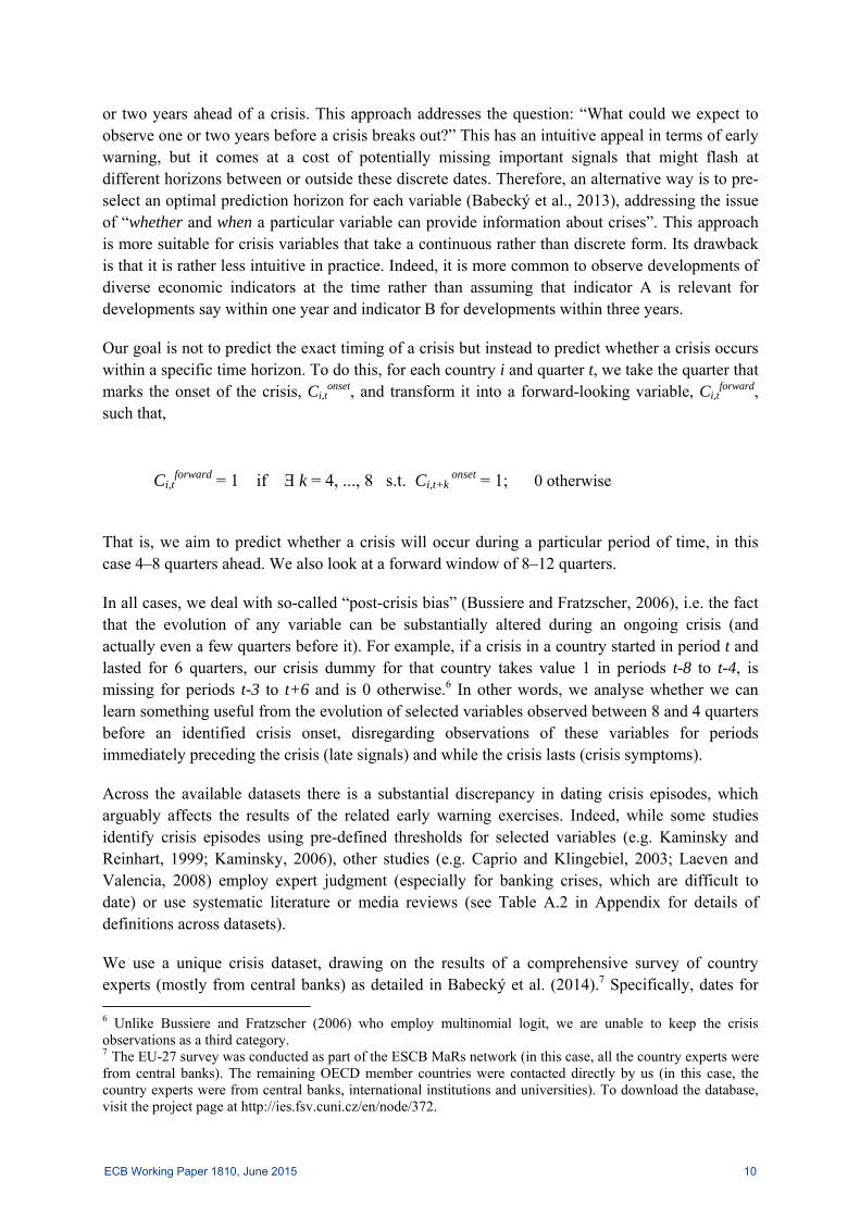
First, we let the RF algorithm identify the most important variables by drawing on 1,000 randomly permuted sub-samples of the data. Of the original set of 20 variables we keep the 10 identified by the RF algorithm as the most important. Figure 1 shows that the current account, the short-term interest rate and the yield curve slope (the 10-year government bond rate minus the short-term interest rate) all appear to be important for predicting banking crises at both short horizons of 4–8 quarters and longer horizons of 8–12 quarters. Short-term interest rates (denoted in Figure 1 as “strate”) are ranked second highest in terms of variable importance for 4–8 quarters, and highest for 8–12 quarters, scoring highly over both horizons in terms of the “mean decrease in the Gini coefficient”, our measure of variable importance. As noted above, we focus mainly on the 4–8 quarter horizon, leaving the 8–12 quarter horizon as a robustness check.

Figure 1: Banking Crises Within 4–8 Quarters (Left) and 8–12 Quarters (Right) – Variable Importance from Random Forest Algorithm

netsavingsgovtdebtnirspreadgovtbalanceunemploymentm3hp_domprivcredityieldcurvestratecuraccount

0 2 4 6 8 10 12

Variable importance: random forest

MeanDecreaseGini

Notes: The figure shows variable importance measured in terms of the mean decrease in the Gini coefficient. Variables are

ordered top-to-bottom from most important to least important. The mean decrease in the Gini coefficient is a measure of how each variable contributes to the homogeneity of the nodes in the resulting random forest (with greater homogeneity equating with better classification of nodes). Each time a particular variable is used to split a node, the Gini coefficients for the child nodes are calculated and compared to that of the original node. The Gini coefficient is a measure of homogeneity from 0 (homogeneous) to 1 (heterogeneous). The changes in the Gini coefficient are summed for each variable and normalised at the end of the calculation. Variables that result in nodes with higher purity will be associated with a larger reduction in the Gini coefficient: a larger decrease implies greater purity.

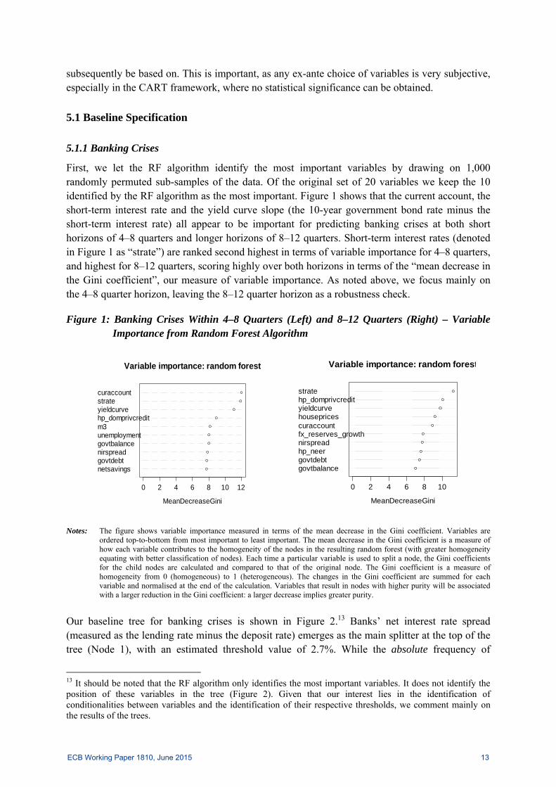
Our baseline tree for banking crises is shown in Figure 2.13 Banks’ net interest rate spread (measured as the lending rate minus the deposit rate) emerges as the main splitter at the top of the tree (Node 1), with an estimated threshold value of 2.7%. While the absolute frequency of

13 It should be noted that the RF algorithm only identifies the most important variables. It does not identify the position of these variables in the tree (Figure 2). Given that our interest lies in the identification of conditionalities between variables and the identification of their respective thresholds, we comment mainly on the results of the trees.

govtbalancegovtdebthp_neernirspreadfx_reserves_growthcuraccounthousepricesyieldcurvehp_domprivcreditstrate

0 2 4 6 8 10


MeanDecreaseGini


banking crises is similar when bank net interest rate spreads are both below and above this threshold (60 quarters signal crisis when net interest rate spreads are low, 72 quarters signal crisis when net spreads are high), the relative frequency of banking crises when banking profitability is low is double (when net spreads are low, there is an 8.9% chance of a banking crisis 4–8 quarters ahead, but when net spreads are high, the chance is 4.3%). The short-term interest rate is on the main left branch of the tree, with a relatively high estimated threshold of 11.26%. Our estimates suggest that when banking sector net interest rate spreads are low and short-term interest rates are high, the probability of a banking crisis 4–8 quarters ahead is 22%. When net interest rate spreads are low and short-term interest rates are low, the probability of crisis is 7%.

Terminal Node 1 identifies 12 episodes of banking crises where net interest rate spreads are low 4–8 quarters ahead of the crisis but where the short-term interest rate does not flag a clear crisis signal (the average short-term interest rate in this sub-sample is 6%). Several crisis onsets in this node belong to the recent turmoil (Austria 2008Q4, France 2008Q1, Hungary 2008Q3, Netherlands 2008Q1, Slovenia 2008Q1, Switzerland 2007Q3, USA 2007Q1) but there are also some banking crises from previous decades (Japan 1997Q3 and 2000Q4, Korea 1997Q1, Switzerland 1991Q1, USA 1982Q1). Terminal Nodes 2 and 3 collect crises episodes that are signalled 4–8 quarters ahead when short-term interest rates are high (greater than 11%) but banks’ net interest rate spreads are low. The terminal current-account split is not entirely enlightening, since on average current accounts are in deficit throughout the crisis period. Terminal Node 2 simply separates the banking crisis in the UK (1991Q1) from the other crisis episodes in Terminal Node 3 (Canada 1993Q1, Italy 1994Q1, Korea 1997Q1, Turkey 2000Q4, 1982Q1).

Figure 2: Banking Crises Within 4–8 Quarters – Binary Tree (Cost of Missing Crisis 7, Best Tree Within 1 Standard Error, Data Priors, Tree Size Depth 3)

STRATE <= 11.26

TerminalNode 1

Class = 0Class Cases %

0 540 93.11 40 6.9

CURACCOUNT <= -2.78

TerminalNode 2


0 51 92.71 4 7.3

CURACCOUNT > -2.78

TerminalNode 3


0 20 55.61 16 44.4

STRATE > 11.26

Node 3Class = 1

CURACCOUNT <= -2.78Class Cases %

0 71 78.01 20 22.0

NIRSPREAD <= 2.69

Node 2Class = 0

STRATE <= 11.26Class Cases %

0 611 91.11 60 8.9

STRATE <= 3.95

TerminalNode 4


0 151 80.71 36 19.3

STRATE > 3.95

TerminalNode 5


0 729 95.71 33 4.3

YIELDCURVE <= 1.34

Node 5Class = 0


0 880 92.71 69 7.3

YIELDCURVE > 1.34

TerminalNode 6


0 733 99.61 3 0.4

NIRSPREAD > 2.69

Node 4Class = 0

YIELDCURVE <= 1.34Class Cases %

0 1613 95.71 72 4.3

Node 1Class = 0

NIRSPREAD <= 2.69Class Cases %

0 2224 94.41 132 5.6

Notes: The tree separates the observations into nodes. The CART algorithm starts with a root node, which is further split into two

child nodes based on classification rules, in our case yes/no questions. Nodes continue to be split until a terminal node is reached.


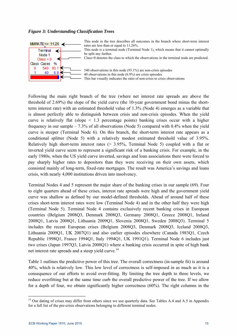
Figure 3: Understanding Classification Trees

This node in the tree describes all outcomes in the branch where short-term interest rates are less than or equal to 11.26%. This node is a terminal node (Terminal Node 1), which means that it cannot optimally be split any further. Class=0 denotes the class to which the observations in the terminal node are predicted. 540 observations in this node (93.1%) are non-crisis episodes 40 observations in this node (6.9%) are crisis episodes This bar visually indicates the ratio of non-crisis to crisis observations

Following the main right branch of the tree (where net interest rate spreads are above the threshold of 2.69%) the slope of the yield curve (the 10-year government bond minus the short-term interest rate) with an estimated threshold value of 1.3% (Node 4) emerges as a variable that is almost perfectly able to distinguish between crisis and non-crisis episodes. When the yield curve is relatively flat (slope < 1.3 percentage points) banking crises occur with a higher frequency in our sample – 7.3% of all observations (Node 5) compared with 0.4% when the yield curve is steeper (Terminal Node 6). On this branch, the short-term interest rate appears as a conditional splitter (Node 5) with a relatively modest estimated threshold value of 3.95%. Relatively high short-term interest rates (> 3.95%, Terminal Node 5) coupled with a flat or inverted yield curve seem to represent a significant risk of a banking crisis. For example, in the early 1980s, when the US yield curve inverted, savings and loan associations there were forced to pay sharply higher rates to depositors than they were receiving on their own assets, which consisted mainly of long-term, fixed-rate mortgages. The result was America’s savings and loans crisis, with nearly 4,000 institutions driven into insolvency.

Terminal Nodes 4 and 5 represent the major share of the banking crises in our sample (69). Four to eight quarters ahead of these crises, interest rate spreads were high and the government yield curve was shallow as defined by our model-defined thresholds. Ahead of around half of these crises short-term interest rates were low (Terminal Node 4) and in the other half they were high (Terminal Node 5). Terminal Node 4 contains exclusively recent banking crises in European countries (Belgium 2008Q3, Denmark 2008Q3, Germany 2008Q1, Greece 2008Q1, Ireland 2008Q1, Latvia 2008Q1, Lithuania 2009Q1, Slovenia 2008Q1, Sweden 2008Q3). Terminal 5 includes the recent European crises (Belgium 2008Q3, Denmark 2008Q3, Iceland 2008Q3, Lithuania 2009Q1, UK 2007Q1) and also earlier episodes elsewhere (Canada 1983Q1, Czech Republic 1998Q1, France 1994Q1, Italy 1994Q1, UK 1991Q1). Terminal Node 6 includes just two crises (Japan 1997Q3, Latvia 2008Q1) where a banking crisis occurred in spite of high bank net interest rate spreads and a steep yield curve.14

Table 1 outlines the predictive power of this tree. The overall correctness (in-sample fit) is around 40%, which is relatively low. This low level of correctness is self-imposed in as much as it is a consequence of our efforts to avoid over-fitting. By limiting the tree depth to three levels, we reduce overfitting but at the same time curb the overall predictive power of the tree. If we allow for a depth of four, we obtain significantly higher correctness (60%). The right columns in the

14 Our dating of crises may differ from others since we use quarterly data. See Tables A.4 and A.5 in Appendix for a full list of the pre-crisis observations belonging to different terminal nodes.


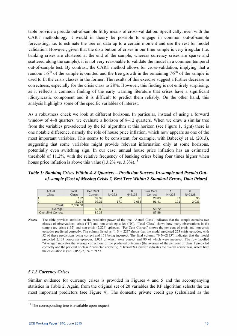
table provide a pseudo out-of-sample fit by means of cross-validation. Specifically, even with the CART methodology it would in theory be possible to engage in common out-of-sample forecasting, i.e. to estimate the tree on data up to a certain moment and use the rest for model validation. However, given that the distribution of crises in our time sample is very irregular (i.e. banking crises are clustered at the end of the sample, whereas currency crises are sparse and scattered along the sample), it is not very reasonable to validate the model in a common temporal out-of-sample test. By contrast, the CART method allows for cross-validation, implying that a random 1/8th of the sample is omitted and the tree growth in the remaining 7/8th of the sample is used to fit the crisis classes in the former. The results of this exercise suggest a further decrease in correctness, especially for the crisis class to 28%. However, this finding is not entirely surprising, as it reflects a common finding of the early warning literature that crises have a significant idiosyncratic component and it is difficult to predict them reliably. On the other hand, this analysis highlights some of the specific variables of interest.

As a robustness check we look at different horizons. In particular, instead of using a forward window of 4–8 quarters, we evaluate a horizon of 8–12 quarters. When we draw a similar tree from the variables pre-selected by the RF algorithm at this horizon (see Figure 1, right) there is one notable difference, namely the role of house price inflation, which now appears as one of the most important variables. This seems to be consistent, for example, with Babecký et al. (2013), suggesting that some variables might provide relevant information only at some horizons, potentially even switching sign. In our case, annual house price inflation has an estimated threshold of 11.2%, with the relative frequency of banking crises being four times higher when house price inflation is above this value (13.2% vs. 3.3%).15

Table 1: Banking Crises Within 4–8 Quarters – Prediction Success In-sample and Pseudo Out-of-sample (Cost of Missing Crisis 7, Best Tree Within 2 Standard Errors, Data Priors)

Actual Class

Total Class

Per Cent Correct

1 N=223

0 N=2133

Per Cent Correct

1 N=228

0 N=2128

1 132 39.39 52 80 28,03 37 950 2,224 92.31 171 2,053 91,41 191 2 033

Total: 2,356.00 Average: 65.85 59,72

Overall % Correct: 89.35 87,86 Notes: The table provides statistics on the predictive power of the tree. “Actual Class” indicates that the sample contains two

classes of observations: crisis (“1”) and non-crisis episodes (“0”). “Total Class” shows how many observations in the sample are crisis (132) and non-crisis (2,224) episodes. “Per Cent Correct” shows the per cent of crisis and non-crisis episodes predicted correctly. The column listed as “1 N = 223” shows that the model predicted 223 crisis episodes, with 52 of these predictions being correct and 171 being incorrect. The final column, “0 N=2133”, indicates that the model predicted 2,133 non-crisis episodes, 2,053 of which were correct and 80 of which were incorrect. The row labelled “Average” indicates the average correctness of the predicted outcomes (the average of the per cent of class 1 predicted correctly and the per cent of class 2 predicted correctly). “Overall % Correct” indicates the overall correctness, where here the calculation is (52+2,053)/2,356 = 89.53.

5.1.2 Currency Crises

Similar evidence for currency crises is provided in Figures 4 and 5 and the accompanying statistics in Table 2. Again, from the original set of 20 variables the RF algorithm selects the ten most important predictors (see Figure 4). The domestic private credit gap (calculated as the

15 The corresponding tree is available upon request.


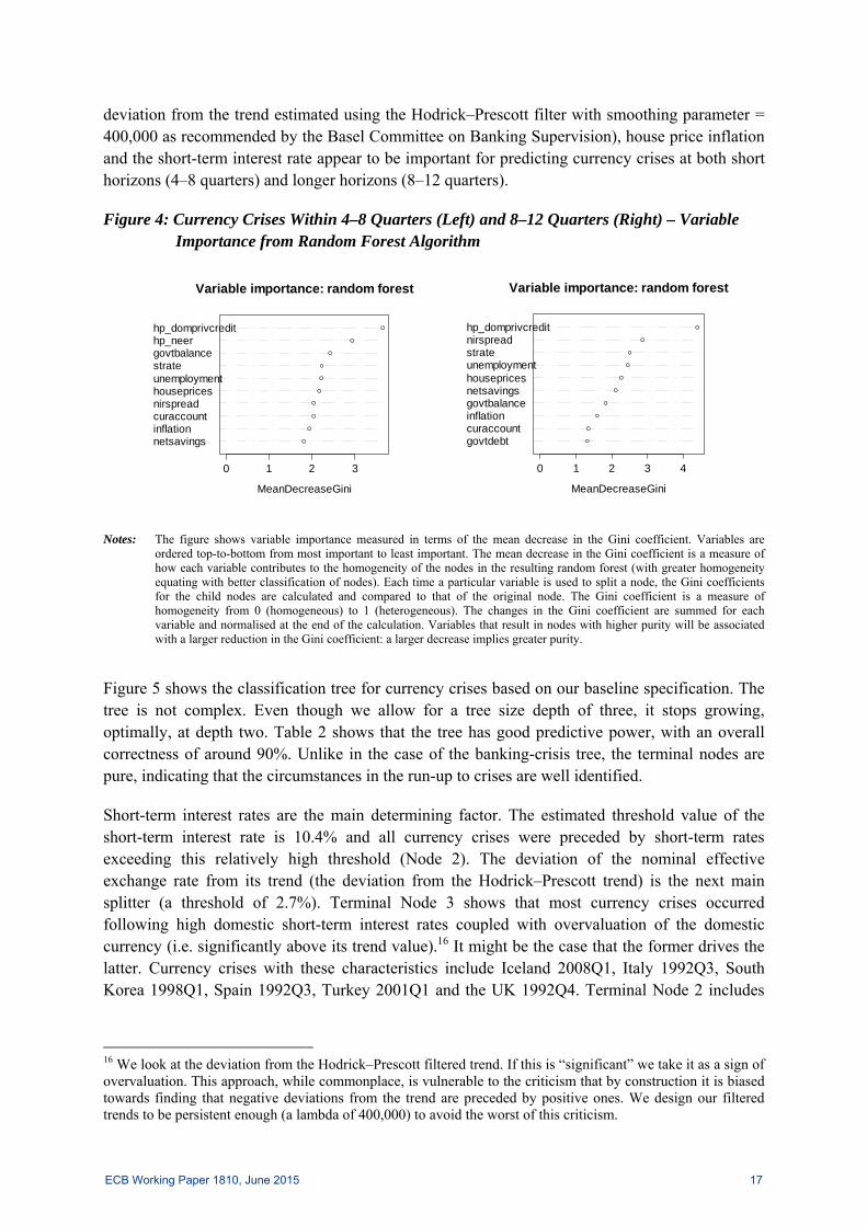
deviation from the trend estimated using the Hodrick–Prescott filter with smoothing parameter = 400,000 as recommended by the Basel Committee on Banking Supervision), house price inflation and the short-term interest rate appear to be important for predicting currency crises at both short horizons (4–8 quarters) and longer horizons (8–12 quarters).

Figure 4: Currency Crises Within 4–8 Quarters (Left) and 8–12 Quarters (Right) – Variable Importance from Random Forest Algorithm

netsavingsinflationcuraccountnirspreadhousepricesunemploymentstrategovtbalancehp_neerhp_domprivcredit

0 1 2 3


MeanDecreaseGini

govtdebtcuraccountinflationgovtbalancenetsavingshousepricesunemploymentstratenirspreadhp_domprivcredit

0 1 2 3 4


MeanDecreaseGini



Figure 5 shows the classification tree for currency crises based on our baseline specification. The tree is not complex. Even though we allow for a tree size depth of three, it stops growing, optimally, at depth two. Table 2 shows that the tree has good predictive power, with an overall correctness of around 90%. Unlike in the case of the banking-crisis tree, the terminal nodes are pure, indicating that the circumstances in the run-up to crises are well identified.

Short-term interest rates are the main determining factor. The estimated threshold value of the short-term interest rate is 10.4% and all currency crises were preceded by short-term rates exceeding this relatively high threshold (Node 2). The deviation of the nominal effective exchange rate from its trend (the deviation from the Hodrick–Prescott trend) is the next main splitter (a threshold of 2.7%). Terminal Node 3 shows that most currency crises occurred following high domestic short-term interest rates coupled with overvaluation of the domestic currency (i.e. significantly above its trend value).16 It might be the case that the former drives the latter. Currency crises with these characteristics include Iceland 2008Q1, Italy 1992Q3, South Korea 1998Q1, Spain 1992Q3, Turkey 2001Q1 and the UK 1992Q4. Terminal Node 2 includes

16 We look at the deviation from the Hodrick–Prescott filtered trend. If this is “significant” we take it as a sign of overvaluation. This approach, while commonplace, is vulnerable to the criticism that by construction it is biased towards finding that negative deviations from the trend are preceded by positive ones. We design our filtered trends to be persistent enough (a lambda of 400,000) to avoid the worst of this criticism.


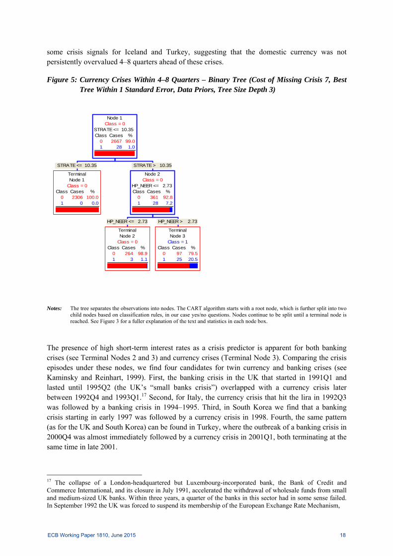
some crisis signals for Iceland and Turkey, suggesting that the domestic currency was not persistently overvalued 4–8 quarters ahead of these crises.

Figure 5: Currency Crises Within 4–8 Quarters – Binary Tree (Cost of Missing Crisis 7, Best Tree Within 1 Standard Error, Data Priors, Tree Size Depth 3)

STRATE <= 10.35

TerminalNode 1


0 2306 100.01 0 0.0

HP_NEER <= 2.73

TerminalNode 2


0 264 98.91 3 1.1

HP_NEER > 2.73

TerminalNode 3


0 97 79.51 25 20.5

STRATE > 10.35

Node 2Class = 0

HP_NEER <= 2.73Class Cases %

0 361 92.81 28 7.2

Node 1Class = 0


0 2667 99.01 28 1.0


child nodes based on classification rules, in our case yes/no questions. Nodes continue to be split until a terminal node is reached. See Figure 3 for a fuller explanation of the text and statistics in each node box.

The presence of high short-term interest rates as a crisis predictor is apparent for both banking crises (see Terminal Nodes 2 and 3) and currency crises (Terminal Node 3). Comparing the crisis episodes under these nodes, we find four candidates for twin currency and banking crises (see Kaminsky and Reinhart, 1999). First, the banking crisis in the UK that started in 1991Q1 and lasted until 1995Q2 (the UK’s “small banks crisis”) overlapped with a currency crisis later between 1992Q4 and 1993Q1.17 Second, for Italy, the currency crisis that hit the lira in 1992Q3 was followed by a banking crisis in 1994–1995. Third, in South Korea we find that a banking crisis starting in early 1997 was followed by a currency crisis in 1998. Fourth, the same pattern (as for the UK and South Korea) can be found in Turkey, where the outbreak of a banking crisis in 2000Q4 was almost immediately followed by a currency crisis in 2001Q1, both terminating at the same time in late 2001.

17 The collapse of a London-headquartered but Luxembourg-incorporated bank, the Bank of Credit and Commerce International, and its closure in July 1991, accelerated the withdrawal of wholesale funds from small and medium-sized UK banks. Within three years, a quarter of the banks in this sector had in some sense failed. In September 1992 the UK was forced to suspend its membership of the European Exchange Rate Mechanism,


Table 2: Currency Crises Within 4–8 Quarters – Prediction Success In-sample and Pseudo Out-of-sample (Cost of Missing Crisis 7, Best Tree Within 2 Standard Errors, Data Priors)

Actual Class

Total Class

Per Cent Correct

1 N=122

0 N=2573

Per Cent Correct

1 N=120

0 N=2575

1 28 89.29 25 3 82.14 23 50 2,667 96.36 97 2,570 96.36 97 2 570

Total: 2,695 Average: 92.82 89.25

Overall % Correct: 96.29 96.22 Notes: The table provides statistics on the predictive power of the tree. “Actual Class” indicates that the sample contains two

classes of observations: crisis (“1”) and non-crisis episodes (“0”). “Total Class” shows how many observations in the sample are crisis (28) and non-crisis (2,667) episodes. “Per Cent Correct” shows the per cent of crisis and non-crisis episodes predicted correctly. The column listed as “1 N = 122” shows that the model predicted 122 crisis episodes, with 25 of these predictions being correct and 97 being incorrect. The final column, “0 N=2573”, indicates that the model predicted 2,573 non-crisis episodes, 2,570 of which were correct and 3 of which were incorrect.

The results suggest that in developed countries currency crises have not typically occurred in the absence of high short-term interest rates and overvalued exchange rates. In this sense, the ability of the tree to pick up conditional relationships between predictors is not really being utilised, as the tree identified two conditions that must be met at the same time. However, the overall predictive power of this tree (Table 2) is substantially higher than in the case of banking crises. Although the episodes of currency crises in our sample of advanced countries were very rare (we have only six currency crises as opposed to approximately 30 episodes of banking crisis), it is still interesting that the nexus between only two variables, i.e. very high short-term interest rates and an overvalued domestic currency, is able to explain most of these episodes. While it is difficult to foresee our estimated threshold of 10% for short-term interest rates being breached by an advanced economy in the future, even under severe stress, it may be relevant for less developed OECD countries and also for emerging countries. The right-hand columns of Table 2 confirm the reliability of this tree by means of pseudo out-of-sample cross-validation, with similar correctness as for the in-sample.

As a robustness check we looked at the longer horizon of 8–12 quarters. When we estimate the tree (available upon request) from the variables pre-selected by the RF algorithm at this horizon (see Figure 1, right) the importance of short-term interest market rates is reaffirmed (albeit with a slightly lower estimated threshold of 9.4%). The nominal exchange rate is not found to be important (not even being part of the variables pre-selected by the RF algorithm). This is supportive of the hypothesis that high short-term interest market rates cause exchange rate overvaluation.18 The government deficit (an estimated threshold of 2.3%) is unable to discriminate well between crisis and non-crisis episodes. Overall, we find that it is difficult to establish good conditional predictors for currency crises at this longer horizon.

For Iceland in 2004–2006, the deviation of domestic private credit from the trend is greater than 50%, arguably also due to the end-point-bias of the Hodrick–Prescott filter used to calculate the trend. The model rightly discards such values.

18 The rise in the short-term interest rate threshold as the crisis approached (9.4% for the 8–12Q horizon vs. 11.4% for the 4–8Q horizon) suggests that short-term rates were increasing in the run-up to the crisis, which might reflect an increase in speculative capital inflows, leading in turn to domestic exchange rate overvaluation.


5.2 Role of Domestic Structural Characteristics

The baseline trees can be further extended. Our first extension is to include variables that have limited variation across time but vary significantly across countries and so represent de-facto structural characteristics of each country. This can (alongside the use of conditional thresholds) further elevate the problem of heterogeneity and poolability. In particular, we consider financial development (“findev”),19 exchange rate regime (“fxregime”), industry share in GDP (“indshare”), overall tax burden (“taxburden”) and trade share in GDP (“trade”). The motivation behind testing these variables as additional predictors of crises is to allow also for long-term vulnerabilities at the country level.

The variable ranking for banking crises, again based on the RF algorithm, for this extended tree is reported in Figure 6. The difference vis-à-vis the original ranking reported in Figure 1 is notable. Structural characteristics play a predominant role at both horizons. Specifically, financial development, economic openness (trade share in GDP) and industry share in GDP have the highest rankings. A country’s financial development, economic openness and industry share can provide important information on the likelihood of a banking crisis 4–8 quarters ahead (Figure 6). A shallow yield curve provides the primary signal. However, structural characteristics are also critical. Specifically, when the yield curve is shallow there are two combinations of structural characteristics that make the economies more vulnerable. First and foremost is the combination of high economic openness (in terms of trade as a share of GDP) and a high degree of financial development (in terms of financial depth). Countries that fall into this category during crisis periods are found in Terminal Node 4 in Figure 7. They include Austria, Belgium, Denmark, Hungary, Ireland, Latvia, Lithuania, the Netherlands, Slovenia, Sweden and Switzerland. In this sub-sample, the relative frequency of banking crises is high (33.8% = 50 crisis cases out of a total of 148 in Terminal Node 4). Second, when trade openness is below the estimated threshold of 94.6%, industry share becomes the next conditional splitter. The relative frequency of crisis is higher (27.9%) when industry share is lower than 23.5% (Terminal Node 1, where we find France, Greece and the UK). Past data suggests, therefore, that when the yield curve is shallow and trade openness is low, having a smaller industrial sector (and possibly but not necessarily a larger financial sector) can leave an economy more vulnerable to banking crises.

19 This variable is defined as the mean of nine variables selected from the World Bank Global Financial Development Database. The entire database features around 70 variables at annual frequency covering different aspects of development of financial systems, such as access, depth, efficiency and stability. While the database includes most of the countries in the world and its span is 1960–2011, it is very unbalanced. We selected nine variables based on availability for our selected set of countries, interpolated them at quarterly frequency and calculated their mean. Most of these variables represent financial depth. These variables are: Bank private credit to GDP (%) – DI.01, Deposit money bank assets to GDP (%) – DI.02, Deposit money bank assets to deposit money bank assets and central bank assets (%) – DI.04, Liquid liabilities to GDP (%) – DI.05, Central bank assets to GDP (%) – DI.06, Financial system deposits to GDP (%) – DI.08, Private credit by deposit money banks and other financial institutions to GDP (%) – DI.12, Bank credit to bank deposits (%) – SI.04, and Bank deposits to GDP (%) – OI.02.


Figure 6: Banking Crises Within 4–8 Guarters (Left) and 8–12 Guarters (Right) – Variable Importance from Random Forest Algorithm for Model Extended to Include Domestic Structural Characteristics

hp_domprivcreditnetsavingstaxburdengovtbalancestrateyieldcurvecuraccountindsharetradefindev

0 5 10 15


MeanDecreaseGini

govtbalancecuraccounttaxburdenstrateyieldcurvetradehousepriceshp_domprivcreditindsharefindev

0 2 4 6 8 10 12


MeanDecreaseGini



Terminal Node 2 captures those banking crises which were preceded by a shallow yield curve and by trade openness below our splitting criterion of 94.6% of GDP and an industry share above the criterion of 23.5% of GDP. Here we mostly find banking crises that occurred prior to the mid-1990s, including Canada 1982Q1, France 1994Q2, Italy 1994Q1, Switzerland 1991Q1, the UK 1991Q1 and the US 1982Q1. The only examples of more recent crises in this node are Germany 200Q1 and Iceland 2008Q3.

Finally, in the right-most branch of this tree, when the slope of the yield curve is above the estimated threshold we also find a few banking crises. Of interest is Terminal Node 6, which contains only crisis episodes (albeit very few), including countries with high financial development (compared with Terminal Node 4). This node includes two banking crises in Japan (1997Q3 and 2000Q4).

Our findings have a number of implications for financial development. First, if the government yield curve is steep, then so long as the country’s level of financial development is anything other than exceptionally high, the odds of a banking crisis within the next 4–8 quarters will be low, at less than one in a hundred (12 divided by 109, from Terminal Node 5). Second, for advanced, open economies, if the yield curve is shallow, less financial development (as opposed to more) has in the past been a better bulwark against the probability of banking crises. This chimes with the findings of Aghion et al. (2004) and with the premise of Rajan (2005) that while a financially deeper economy may take on more risks these risks can be restrained by both monetary and macroprudential policy.

Our findings on financial development are, we acknowledge, weakened by the fact that some financial development during a boom will always be temporary rather than structural (Hansen and Sulla, 2013) and therefore a symptom of the boom rather than a reliable predictor. A smaller, but


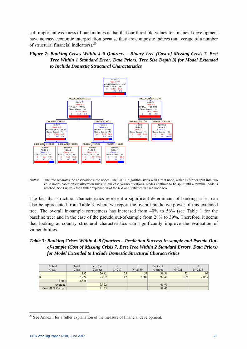
still important weakness of our findings is that that our threshold values for financial development have no easy economic interpretation because they are composite indices (an average of a number of structural financial indicators).20

Figure 7: Banking Crises Within 4–8 Quarters – Binary Tree (Cost of Missing Crisis 7, Best Tree Within 1 Standard Error, Data Priors, Tree Size Depth 3) for Model Extended to Include Domestic Structural Characteristics

INDSHARE <= 23.56

TerminalNode 1


0 44 72.11 17 27.9

INDSHARE > 23.56

TerminalNode 2


0 965 95.81 42 4.2

TRADE <= 94.65

Node 3Class = 0

INDSHARE <= 23.56Class Cases %

0 1009 94.51 59 5.5

FINDEV <= 57.06

TerminalNode 3


0 120 97.61 3 2.4

FINDEV > 57.06

TerminalNode 4


0 98 66.21 50 33.8

TRADE > 94.65

Node 4Class = 1

FINDEV <= 57.06Class Cases %

0 218 80.41 53 19.6

YIELDCURVE <= 1.37

Node 2Class = 0

TRADE <= 94.65Class Cases %

0 1227 91.61 112 8.4

FINDEV <= 150.88

TerminalNode 5


0 997 98.81 12 1.2

FINDEV > 150.88

TerminalNode 6


0 0 0.01 8 100.0

YIELDCURVE > 1.37

Node 5Class = 0


0 997 98.01 20 2.0

Node 1Class = 0


0 2224 94.41 132 5.6


child nodes based on classification rules, in our case yes/no questions. Nodes continue to be split until a terminal node is reached. See Figure 3 for a fuller explanation of the text and statistics in each node box.

The fact that structural characteristics represent a significant determinant of banking crises can also be appreciated from Table 3, where we report the overall predictive power of this extended tree. The overall in-sample correctness has increased from 40% to 56% (see Table 1 for the baseline tree) and in the case of the pseudo out-of-sample from 28% to 39%. Therefore, it seems that looking at country structural characteristics can significantly improve the evaluation of vulnerabilities.

Table 3: Banking Crises Within 4–8 Quarters – Prediction Success In-sample and Pseudo Out-of-sample (Cost of Missing Crisis 7, Best Tree Within 2 Standard Errors, Data Priors) for Model Extended to Include Domestic Structural Characteristics

Actual Class

Total Class

Per Cent Correct

1 N=217

0 N=2139

Per Cent Correct

1 N=221

0 N=2135

1 132 56.82 75 57 39.39 52 800 2,224 93.62 142 2,082 92.40 169 2 055

Total: 2,356 Average: 75.22 65.90

Overall % Correct: 91.55 89.43

20 See Annex I for a fuller explanation of the measure of financial development.


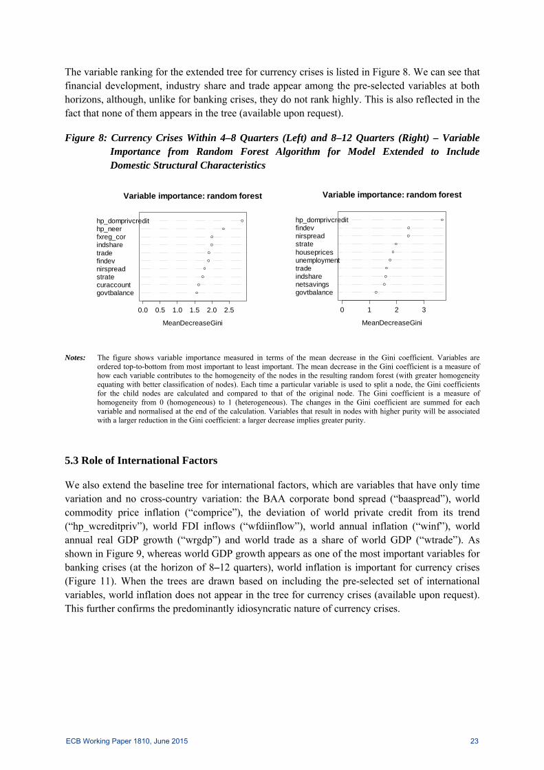
The variable ranking for the extended tree for currency crises is listed in Figure 8. We can see that financial development, industry share and trade appear among the pre-selected variables at both horizons, although, unlike for banking crises, they do not rank highly. This is also reflected in the fact that none of them appears in the tree (available upon request).

Figure 8: Currency Crises Within 4–8 Quarters (Left) and 8–12 Quarters (Right) – Variable Importance from Random Forest Algorithm for Model Extended to Include Domestic Structural Characteristics

govtbalancecuraccountstratenirspreadfindevtradeindsharefxreg_corhp_neerhp_domprivcredit

0.0 0.5 1.0 1.5 2.0 2.5


MeanDecreaseGini

govtbalancenetsavingsindsharetradeunemploymenthousepricesstratenirspreadfindevhp_domprivcredit

0 1 2 3


MeanDecreaseGini

Notes: The figure shows variable importance measured in terms of the mean decrease in the Gini coefficient. Variables are ordered top-to-bottom from most important to least important. The mean decrease in the Gini coefficient is a measure of how each variable contributes to the homogeneity of the nodes in the resulting random forest (with greater homogeneity equating with better classification of nodes). Each time a particular variable is used to split a node, the Gini coefficients for the child nodes are calculated and compared to that of the original node. The Gini coefficient is a measure of homogeneity from 0 (homogeneous) to 1 (heterogeneous). The changes in the Gini coefficient are summed for each variable and normalised at the end of the calculation. Variables that result in nodes with higher purity will be associated with a larger reduction in the Gini coefficient: a larger decrease implies greater purity.

5.3 Role of International Factors

We also extend the baseline tree for international factors, which are variables that have only time variation and no cross-country variation: the BAA corporate bond spread (“baaspread”), world commodity price inflation (“comprice”), the deviation of world private credit from its trend (“hp_wcreditpriv”), world FDI inflows (“wfdiinflow”), world annual inflation (“winf”), world annual real GDP growth (“wrgdp”) and world trade as a share of world GDP (“wtrade”). As shown in Figure 9, whereas world GDP growth appears as one of the most important variables for banking crises (at the horizon of 8–12 quarters), world inflation is important for currency crises (Figure 11). When the trees are drawn based on including the pre-selected set of international variables, world inflation does not appear in the tree for currency crises (available upon request). This further confirms the predominantly idiosyncratic nature of currency crises.


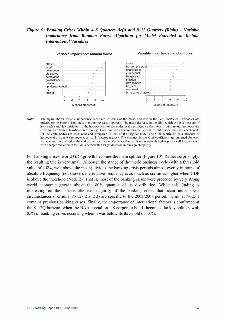
Figure 9: Banking Crises Within 4–8 Quarters (left) and 8–12 Quarters (Right) – Variable Importance from Random Forest Algorithm for Model Extended to Include International Variables

hhdebtm3hp_domprivcreditinflationgovtbalancenetsavingsyieldcurvecuraccountwrgdpstrate

0 2 4 6 8 10


MeanDecreaseGini

fx_reserves_growthnirspreadhp_neergovtbalanceinflationbaaspreadcuraccounthousepriceshp_domprivcreditstrate

0 2 4 6 8 10


MeanDecreaseGini


For banking crises, world GDP growth becomes the main splitter (Figure 10). Rather surprisingly, the resulting tree is very small. Although the stance of the world business cycle (with a threshold value of 4.8%, well above the mean) divides the banking crisis periods almost evenly in terms of absolute frequency (not shown), the relative frequency is as much as six times higher when GDP is above the threshold (Node 2). That is, most of the banking crises were preceded by very strong world economic growth above the 80% quantile of its distribution. While this finding is interesting on the surface, the vast majority of the banking crises that occur under these circumstances (Terminal Nodes 2 and 3) are specific to the 2007/2008 period. Terminal Node 1 contains previous banking crises. Finally, the importance of international factors is confirmed at the 8–12Q horizon, when the BAA spread on US corporate bonds becomes the key splitter, with 85% of banking crises occurring when it was below its threshold of 1.6%.


Figure 10: Banking Crises Within 4–8 Quarters – Binary Tree (Cost of Missing Crisis 7, Best Tree Within 1 Standard Error, Data Priors, Tree Size Depth 3) for Model Extended to Include International Variables

WRGDP <= 4.84

TerminalNode 1


0 1875 96.91 60 3.1

YIELDCURVE <= 1.37

TerminalNode 2


0 218 76.21 68 23.8

YIELDCURVE > 1.37

TerminalNode 3


0 131 97.01 4 3.0

WRGDP > 4.84

Node 2Class = 1


0 349 82.91 72 17.1

Node 1Class = 0

WRGDP <= 4.84Class Cases %

0 2224 94.41 132 5.6

Notes: The tree separates the observations into nodes. The CART algorithm starts with a root node, which is further split into two child nodes based on classification rules, in our case yes/no questions. Nodes continue to be split until a terminal node is reached. See Figure 3 for a fuller explanation of the text and statistics in each node box.

The incorporation of international variables improves the overall predictive power of the tree (Table 4) vis-à-vis the baseline tree (Table 1) from 40% to 51% for the in-sample and from 28% to 42% for the pseudo out-of-sample. While the improvement is less than in the case of the tree augmented by structural characteristics, it is very respectable given that the tree is very sparse. Therefore, it can be concluded that in predicting banking crises in developed countries there is interplay not only between domestic short-term developments and domestic structural characteristics, but also between domestic and international developments. Specifically, the world business cycle is a significant predictor of banking crises precisely because banking crises are often clustered over time. This is not the case for currency crises, at least for advanced countries.


Table 4: Banking Crises Within 4–8 Quarters – Prediction Success In-sample and Pseudo Out-of-sample (Cost of Missing Crisis 7, Best Tree within 2 Standard Errors, Data Priors) for Model Extended to Include International Variables

Actual Class

Total Class

Per Cent Correct

1 N=286

0 N=2070

Per Cent Correct

1 N=236

0 N=2120

1 132 51.52 68 64 41.67 55 770 2,224 90.20 218 2,006 91.86 181 2 043

Total: 2,356 Average: 70.86 66.76

Overall % Correct: 88.03 89.05

Figure 11: Currency Crises Within 4–8 Quarters (Left) and 8–12 Quarters (Right) – Variable Importance from Random Forest Algorithm for Model Extended to Include International Variables

bank_profnetsavingswinfinflationhousepricesunemploymentgovtbalancemmratehp_neerhp_domprivcredit

0 1 2 3


MeanDecreaseGini

termsoftradegovtbalancehousepricesinflationunemploymentnetsavingsmmratewinfbank_profhp_domprivcredit

0 1 2 3 4


MeanDecreaseGini


6. Robustness Checks

Like the results of any early warning exercise, our results are conditioned on our country and time coverage and on our choice of potential leading indicators. In this section we provide three robustness checks, the first related to country coverage, the second related to time coverage and the third related to the choice of potential leading indicators. We run this robustness check only for banking crises (and a horizon of 4–8 quarters) given that they imply a reduction in crisis episodes. This makes the analysis for currency crises, whose number is reduced even in the baseline sample, unfeasible.

First, we drop countries that can still (in spite of their EU and/or OECD membership) be considered emerging economies. This applies to the ten new EU member states from Central and


Eastern Europe and also to Israel, Korea Mexico and Turkey. We first run the RF algorithm to pre-select the variables and then draw a tree. As we can see in Figure 12, this way our effective sample of banking crisis episodes decreases to 22, but the share of occurrence of banking crises in the overall sample remains very similar (5.9% vs. 5.6%). The results are largely consistent with those for the full sample (Figures 1 and 2). The slope of the yield curve and the short-term interest rate are the main crisis forerunners. Whereas the net interest rate spread ceases to be important, the domestic credit gap makes it into the tree. However, its estimated threshold and the sample split it implies do not provide any useful information.

Figure 12: Banking Crises Within 4–8 Quarters – Binary Tree (Cost of Missing Crisis 7, Best Tree Within 1 Standard Error, Data Priors, Tree Size Depth 3) and Variable Importance from Random Forest Algorithm – “Emerging” Countries Dropped

HP_DOMPRIVCREDIT <= -6.40

TerminalNode 1


0 177 99.41 1 0.6

STRATE <= 4.22

TerminalNode 2


0 174 79.51 45 20.5

STRATE > 4.22

TerminalNode 3


0 498 92.61 40 7.4

HP_DOMPRIVCREDIT > -6.40

Node 3Class = 0


0 672 88.81 85 11.2

YIELDCURVE <= 1.37

Node 2Class = 0

HP_DOMPRIVCREDIT <= -6.40Class Cases %

0 849 90.81 86 9.2

YIELDCURVE > 1.37

TerminalNode 4


0 727 98.21 13 1.8

Node 1Class = 0


0 1576 94.11 99 5.9

govtdebthp_neerhhdebtunemploymentm3inflationhp_domprivcreditcuraccountstrateyieldcurve

0 2 4 6 8 10


MeanDecreaseGini


In our second check we drop all the observations relating to the recent global financial crisis (but conversely keep the original country span). As we can see in Figure 13, this way our effective sample of banking crises episodes decreases to 23, but the share of occurrence of banking crises in the overall sample remains very similar (5.3% vs. 5.6%). The results are again largely consistent with those for full sample (Figures 1 and 2). In this case, the net interest rate spread keeps its relevance as the main spiller, with a practically identical threshold value (2.8% vs. 2.69%). This confirms that our baseline results are robust even when we disregard the recent financial crisis.

Figure 13: Banking Crises Within 4–8 Quarters – Binary Tree (Cost of Missing Crisis 7, Best Tree Within 1 Standard Error, Data Priors, Tree Size Depth 3) and Variable Importance from Random Forest Algorithm – Observations from 2007 Onwards Dropped

STRATE <= 1.63

TerminalNode 1


0 19 59.41 13 40.6

STRATE <= 11.26

TerminalNode 2


0 434 95.81 19 4.2

STRATE > 11.26

TerminalNode 3


0 65 76.51 20 23.5

STRATE > 1.63

Node 3Class = 0


0 499 92.81 39 7.2

NIRSPREAD <= 2.80

Node 2Class = 0


0 518 90.91 52 9.1

NIRSPREAD > 2.80

TerminalNode 4


0 1302 96.41 49 3.6

Node 1Class = 0

NIRSPREAD <= 2.80Class Cases %

0 1820 94.71 101 5.3

fx_reserves_growthnirspreadnetsavingsgovtdebtgovtbalanceyieldcurvem3hp_domprivcreditcuraccountstrate

0 2 4 6 8 10

Variable importance: random fores

MeanDecreaseGini

In the third check, we pool all the potential crisis forerunners, i.e. besides the domestic variables we also include the domestic structural characteristics and international variables. When we compare the results with the extended models in Figures 6 and 7 (domestic structural characteristics) and Figures 9 and 10 (international variables) we find that whereas domestic structural characteristics (financial development, trade to GDP and industry share) seem to dominate international variables as crisis forerunners, world GDP growth retains its value of main splitter with the same threshold value as in Figure 9, confirming that the relative occurrence of banking crises is several times higher when preceded by strong world economic growth. Whereas the role of domestic short-term (non-structural) variables is significantly muted in this case, the short-term interest rate and yield curve slope retain their status as the most informative domestic variables.


Figure 14: Banking Crises Within 4–8 Quarters – Binary Tree (Cost of Missing Crisis 7, Best Tree Within 1 Standard Error, Data Priors, Tree Size Depth 3) and Variable Importance from Random Forest Algorithm – for Model Extended to Include Domestic Structural Characteristics and International Variables

FINDEV <= 150.88

TerminalNode 1


0 1581 99.01 16 1.0

FINDEV > 150.88

TerminalNode 2


0 0 0.01 8 100.0

STRATE <= 9.83

Node 3Class = 0


0 1581 98.51 24 1.5

TRADE <= 59.65

TerminalNode 3


0 178 83.61 35 16.4

TRADE > 59.65

TerminalNode 4


0 116 99.11 1 0.9

STRATE > 9.83

Node 4Class = 0


0 294 89.11 36 10.9

WRGDP <= 4.84

Node 2Class = 0


0 1875 96.91 60 3.1

INDSHARE <= 23.56

TerminalNode 5


0 17 58.61 12 41.4

INDSHARE > 23.56

TerminalNode 6


0 199 100.01 0 0.0

TRADE <= 78.54

Node 6Class = 0

INDSHARE <= 23.56Class Cases %

0 216 94.71 12 5.3

YIELDCURVE <= 1.51

TerminalNode 7


0 80 58.01 58 42.0

YIELDCURVE > 1.51

TerminalNode 8


0 53 96.41 2 3.6

TRADE > 78.54

Node 7Class = 1


0 133 68.91 60 31.1

WRGDP > 4.84

Node 5Class = 1


0 349 82.91 72 17.1

Node 1Class = 0

WRGDP <= 4.84Class Cases %

0 2224 94.41 132 5.6

hp_domprivcreditnetsavingstaxburdenyieldcurvestratecuraccountwrgdptradeindsharefindev

0 2 4 6 8 10 12


MeanDecreaseGini

We believe that these checks broadly confirm the robustness of our baseline results, as the latter seem not to be altered by the presence of countries that may still be deemed emerging or when we disregard observations relating to the global financial crises. Whereas it seems that a significant part of a country’s vulnerability to banking crises is determined by its structural characteristics, which change only slowly over time, there are several robust indicators whose short-term developments may be useful. Most notably, all these variables – the short-term interest rate, the net interest rate spread and the slope of the yield curve – relate to interest rate developments.

7. Comparisons with Other Studies

While we believe our results corroborate many of the findings of other researchers, it is important to note where they do not. Most notably in the case of banking crises, the credit-to-GDP gap (the Basel gap), which is probably the most prominent variable in most previous studies, does not play an important role in our exercise. Recently, for instance, Drehmann and Juselius (2014) argue that the domestic credit gap is perhaps the single most important indicator of banking crises one to four years ahead. That our results suggest otherwise may be explained in part by differences in prediction horizons, which in our case are shorter. However, even Babecký et al. (2014), who use a linear probability model (nested within a Bayesian model averaging approach) based on similar prediction horizons and even a similar dataset, still find that the credit gap plays an important role in crisis prediction.21 Therefore, a more fundamental cause of disagreement may be that the credit-

21 David and Karim (2008b) find procyclical behaviour of credit growth. Specifically, credit growth generates credit risk during the boom phase up to four years prior to a crisis; at the shorter horizon credit rationing occurs, increasing the likelihood of crisis. In fact, there might even be interplay with the existence of deposit insurance, given that it increases moral hazard, which in turn increases credit risk during the boom phase, in line with previous evidence by Demirgüç-Kunt and Detragiache (1998).


to-GDP gap is commonly assumed to be an unconditional signal of crisis, whereas our work finds that signals are highly conditional. For example, one country may have a booming banking sector (in terms of net interest rate spreads) but a negligible probability of banking crisis; another may have an equally frothy banking sector but may be running a high risk of crisis. The reason is that the risk of crisis is conditional on other factors, namely the steepness of the yield curve, the level of short-term interest rates and, in some instances, the size of the current account balance. On the other hand, Alessi and Detken (2014) recently find threshold values for more nuanced credit variables in a very similar empirical framework to ours.22

These results can also be compared with previous studies using binary trees for analysing banking crises in emerging market economies (Dattagupta and Cashin, 2011; Davis et al. 2011). We confirm the importance of falling banking-sector profitability, which in our case can, with some generalisation, be proxied by net interest rate spreads, as well as a high level of financial intermediation (we use a broader category of financial development that averages over a number of structural measures), but discard the relevance of some other indicators, such as high inflation and deposit dollarisation. These developments were much less common in advanced countries.

Our results for currency crises in turn confirm the role of exchange rate overvaluation. We do not find a role for the current account, which is another prominent variable found in previous studies focusing on currency crises (e.g. Bussiere, 2013a).23 However, these studies are aimed almost exclusively at emerging countries, which may itself be a reason for the discrepancy. Interestingly, the current account appears in our exercise even among the variables pre-selected by the RF algorithm (in the baseline tree and the tree augmented by foreign variables at the shorter horizon) but does not make it into the tree. The potential unconditionality of this variable (as in the case of the domestic credit gap for banking crises) may offer a potential explanation. On the other hand, Ghosh and Ghosh (2003), who study currency crises in emerging countries using binary trees, confirm the relevance of the current account balance as well as other factors such as high external sovereign debt and high corruption, which are much less relevant for advanced countries. Therefore, our finding of high short-term interest rates and previous currency overvaluation is partially novel.

To shed further light on the issue of whether our results are driven by a different dataset or a different empirical method, we cast our dataset into the common logit model. However, it should be noted that the scope of comparability between logit and CART is limited because (i) while logit draws on the full set of potential indicators, our CART draws on a very limited set of variables, as they are first pre-selected by the RF routine and then nested in the tree, (ii) logit drops missing values whereas CART works with them, and (iii) CART uses a pooled sample, whereas logit makes use of a panel data structure. Therefore, to make the comparison reasonable we cast the set of variables pre-selected by the RF algorithm into logit and use a pooled sample rather than a panel (i.e. we do not account for unobserved heterogeneity by means of fixed effects).

22 However, the fact that this study finds that credit plays a role is not entirely surprising, as around 40% of all the variables considered in the analysis are credit-related. 23 Due to data unavailability we are unable to consider another variable common in studies of currency crises in emerging countries, namely the ratio of short-term debt to reserves.


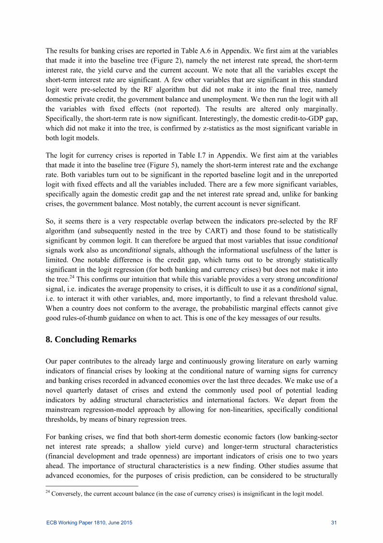
The results for banking crises are reported in Table A.6 in Appendix. We first aim at the variables that made it into the baseline tree (Figure 2), namely the net interest rate spread, the short-term interest rate, the yield curve and the current account. We note that all the variables except the short-term interest rate are significant. A few other variables that are significant in this standard logit were pre-selected by the RF algorithm but did not make it into the final tree, namely domestic private credit, the government balance and unemployment. We then run the logit with all the variables with fixed effects (not reported). The results are altered only marginally. Specifically, the short-term rate is now significant. Interestingly, the domestic credit-to-GDP gap, which did not make it into the tree, is confirmed by z-statistics as the most significant variable in both logit models.

The logit for currency crises is reported in Table I.7 in Appendix. We first aim at the variables that made it into the baseline tree (Figure 5), namely the short-term interest rate and the exchange rate. Both variables turn out to be significant in the reported baseline logit and in the unreported logit with fixed effects and all the variables included. There are a few more significant variables, specifically again the domestic credit gap and the net interest rate spread and, unlike for banking crises, the government balance. Most notably, the current account is never significant.

So, it seems there is a very respectable overlap between the indicators pre-selected by the RF algorithm (and subsequently nested in the tree by CART) and those found to be statistically significant by common logit. It can therefore be argued that most variables that issue conditional signals work also as unconditional signals, although the informational usefulness of the latter is limited. One notable difference is the credit gap, which turns out to be strongly statistically significant in the logit regression (for both banking and currency crises) but does not make it into the tree.24 This confirms our intuition that while this variable provides a very strong unconditional signal, i.e. indicates the average propensity to crises, it is difficult to use it as a conditional signal, i.e. to interact it with other variables, and, more importantly, to find a relevant threshold value. When a country does not conform to the average, the probabilistic marginal effects cannot give good rules-of-thumb guidance on when to act. This is one of the key messages of our results.

8. Concluding Remarks

Our paper contributes to the already large and continuously growing literature on early warning indicators of financial crises by looking at the conditional nature of warning signs for currency and banking crises recorded in advanced economies over the last three decades. We make use of a novel quarterly dataset of crises and extend the commonly used pool of potential leading indicators by adding structural characteristics and international factors. We depart from the mainstream regression-model approach by allowing for non-linearities, specifically conditional thresholds, by means of binary regression trees.

For banking crises, we find that both short-term domestic economic factors (low banking-sector net interest rate spreads; a shallow yield curve) and longer-term structural characteristics (financial development and trade openness) are important indicators of crisis one to two years ahead. The importance of structural characteristics is a new finding. Other studies assume that advanced economies, for the purposes of crisis prediction, can be considered to be structurally 24 Conversely, the current account balance (in the case of currency crises) is insignificant in the logit model.


homogeneous. Typically the assumption is made that advanced economies are structurally distinct only from emerging economies, not from each other. However, we find that structural differences between advanced economies offer important information on how vulnerable a country is to a banking crisis, with economies that are more financially developed being sometimes but not always more vulnerable (depending on a number of prevailing macroeconomic factors), and likewise with trade openness – more open can mean more vulnerable if the government yield curve is shallow. The parallels with emerging economies are, in other words, stronger than we may have previously presumed (Eichengreen, 2010).

We find that the most important signals of currency crises are short-term and country-specific: high short-term rates and an overvalued currency are the most important predictors of crisis. Structural characteristics of the domestic economy are not important (contrary to the findings of, for instance, Frost and Saiki, 2013), nor are international factors such as the global business cycle (a finding that, once we abstract from contagion, is consistent with most other studies of currency crisis).

Our findings have implications for the recent debate on macroprudential policy. First, our results in a broad sense suggest that not all early warning indicators are reliable for all countries all of the time, and the estimated thresholds can be conditional (on other thresholds). This suggests that an indicator’s conditionality and broader country-specific characteristics should be taken into account in supranational financial stability surveillance bodies such as the Financial Stability Board (FSB) and the European Systemic Risk Board (ESRB). For example, we found that bank net interest rate spreads often indicated forthcoming banking crises, but looking at this indicator unconditionally can be misleading because numerous banking crises also occurred when net interest rate spreads were high. Second, although we provide thresholds for several indicators, it should also be kept in mind that any threshold is subject to substantial uncertainty. Therefore, there is no sharp cutting edge between crisis-prone and non-crisis-prone situations. Finally, our results suggest that information on the domestic credit gap, which has been suggested by the Basel Committee on Banking Supervision (BCBS) as a key tool for activating the countercyclical capital buffer (CCCB), should be used with caution. Specifically, this indicator does not flash as a core leading indicator of crises (either banking or currency) when conditionality is taken into account, and it is impossible to find any reliable threshold for it.


References

ALESSI, L. AND C. DETKEN (2013): “Quasi Real Time Early Warning Indicators for Costly Asset Price Boom/bust Cycles: A Role for Global Liquidity.”, European Journal of Political Economy 27(3), pp. 520–533.

ALESSI, L. AND C. DETKEN (2014): “Identifying Excessive Credit Growth and Leverage.” ECB Working Paper No. 1723.

ADRIAN, T., A. ESTRELLA, AND H. SHIN (2010): “Monetary Cycles, Financial Cycles and the Business Cycle.” Federal Reserve Bank of New York Staff Reports, No. 421.

AGHION, P., P. BACCHETTA, AND A. BANERJEE (2004): “Financial Development and the Instability of Open Economies.” Journal of Monetary Economics 51, pp. 1077–1106.

ARTETA, C. AND B. EICHENGREEN (2000): “Banking Crises in Emerging Markets: Presumptions and Evidence.” Center for International and Development Economics Research, University of California at Berkeley, Working Paper No. C00-115.

BABECKÝ, J., T. HAVRÁNEK, J. MATĚJŮ, M. RUSNÁK, K. ŠMÍDKOVÁ, AND B. VAŠÍČEK (2014): “Banking, Debt, and Currency Crises in Developed Countries: Stylized Facts and Early Warning Indicators.” Journal of Financial Stability 15, pp. 1–17.

BABECKÝ, J., T. HAVRÁNEK, J. MATĚJŮ, M. RUSNÁK, K. ŠMÍDKOVÁ, AND B. VAŠÍČEK (2013): “Leading Indicators of Crisis Incidence: Evidence from Developed Countries.” Journal of International Money and Finance 35, pp. 1–19.

BORIO, C. AND P. LOWE (2002): “Asset Prices, Financial and Monetary Stability: Exploring the Nexus.” BIS Working Paper No. 114.

BORIO, C. AND M. DREHMANN (2009): “Towards an Operational Framework for Financial Stability: ‘Fuzzy’ Measurement and Its Consequences.”, BIS Working Paper No. 284.

BREIMAN, L., J. FRIEDMAN, R. OLSHEN, AND C. STONE (1984): Classification and Regression Trees, Chapman & Hall, London.

BUSSIERE, M. (2013A): “In Defense of Early Warning Indicators.” Banque de France Working Paper No. 713.

BUSSIERE, M. (2013B): “Balance of Payment Crises in Emerging Markets – How Early were the “Early” Warning Signals?” Applied Economics 45, pp. 1601–1623.

BUSSIERE, M. AND M. FRATZSCHER (2006): “Towards a New Early Warning System of Financial Crises.”, Journal of International Money and Finance 25(6), pp. 953–973.

CAPRIO, G. AND D. KLINGEBIEL (2003): “Episodes of Systemic and Borderline Financial Crises.”, World Bank, January 22. http://go.worldbank.org/5DYGICS7B0.

CHAMON, M., P. MANASE AND A. PRATI (2007): “Can We Predict the Next Capital Account Crisis?” IMF Staff Papers 54(2), pp. 270–305.

CRESPO CUARESMA, J. AND T. SLACIK (2009): “On the Determinants of Currency Crises: The Role of Model Uncertainty.” Journal of Macroeconomics 31(4), pp. 621–632.

DATTAGUPTA, R. AND P. CASHIN (2011): “Anatomy of Banking Crises in Developing and Emerging Market Countries.” Journal of International Money and Finance 30, pp. 354–376.

DAVIS, E. P. AND D. KARIM (2008a): “Could Early Warning Systems Have Helped To Predict the Sub-Prime Crisis?” National Institute Economic Review 206, pp. 35–47.


DAVIS, E. P. AND D. KARIM (2008b): “Comparing Early Warning Systems for Banking Crises.” Journal of Financial Stability 4(2), pp. 89–120.

DAVIS, E. P., D. KARIM AND I. LIADZE (2011): “Should Multivariate Early Warning Systems for Banking Crises Pool Across Regions?” Review of World Economics 147, pp. 693–716.

DEMIRGÜÇ-KUNT, A. AND E. DETRAGIACHE (1998): “The Determinants of Banking Crises in Developing and Developed Countries.” IMF Staff Papers 45(1), pp. 81–109.

DEMIRGÜÇ-KUNT, A. AND E. DETRAGIACHE (2005): “Cross-Country Empirical Studies of Systemic Bank Distress: A Survey.” IMF Working Paper No. 05/96.

DREHMANN, M. AND M. JUSELIUS (2014): “Evaluating Early Warning Indicators of Banking Crises: Satisfying Policy Requirements.” International Journal of Forecasting 30(3), pp. 759–780.

EICHENGREEN, B. (2010): “Managing Openness: Lessons from the Crisis for Emerging Markets.” in Haddad, M. and B. Shepherd (eds.): Managing Openness: Trade and Outward Oriented Growth after the Crisis, World Bank, Washington DC.

FRANKEL, J. A. AND S.-J. WEI (2004): “Managing Macroeconomic Crises.” NBER Working Paper No. 10907.

FROST, J. AND A. SAIKI (2013): “Early Warning for Currency Crises: What is the Role of Financial Openness.”, DNB Working Paper No. 373.

GHOSH, S. R. AND A. R. GHOSH (2003): “Structural Vulnerabilities and Currency Crises.” IMF Staff Papers 50(3), pp. 481–506.

HANSEN, N-J. AND O. SULLA (2013): “Credit Growth in Latin America: Financial Development or Credit Boom?” IMF Working Paper WP/13/106.

KAMINSKY, G. L. (2006): “Currency Crises: Are They All the Same?” Journal of International Money and Finance 25(3), pp. 503–527.

KAMINSKY, G. L. AND C. M. REINHART (1999): “The Twin Crises: The Causes of Banking and Balance-of-Payments Problems.” American Economic Review 89(3), pp. 473–500.

LAEVEN, L. AND F. VALENCIA (2008): “Systemic Banking Crises: A New Database.”, IMF Working Paper No. 08/224.

LAEVEN, L. AND F. VALENCIA (2010): “Resolution of Banking Crises: The Good, the Bad, and the Ugly.”, IMF Working Paper No. 10/146.

LAEVEN, L. AND F. VALENCIA (2012): “Systemic Banking Crises Database: An Update.” IMF Working Paper No. 12/163.

LIAW, A. AND M. WEINER (2002): “Classification and Regression by Random Forest.” R News Vol. 2/3 (December 2002), pp. 18–22.

MANASSE, P., N. ROUBINI, AND A. SCHIMMELPFENNIG (2003): “Predicting Sovereign Debt Crises.” IMF Working Paper No. 03/221.

MANASSE, P. AND N. ROUBINI (2009): “Rules of Thumb” for Sovereign Debt Crises.” Journal of International Economics 78, pp. 192–205.

RAJAN, R. (2005): "Has Financial Development Made the World Riskier?" NBER Working Paper Series, No.11728.

REINHART, C. M. AND K. S. ROGOFF (2008): “Banking Crises: An Equal Opportunity Menace.”, NBER Working Paper No. 14587.


REINHART, C. M. AND K. S. ROGOFF (2011): “From Financial Crash to Debt Crisis.” American Economic Review 101(5), pp. 1676–1706.

ROSE, A. K. (2011): “Exchange Rate Regimes in the Modern Era: Fixed, Floating, and Flaky.” Journal of Economic Literature 49(3), pp. 652–672.

SAVONA, R. AND M. VEZZOLI (2012): “Multidimensional Distance-to-Collapse Point and Sovereign Default Prediction.” Intelligent Systems in Accounting, Finance and Management 19(4), pp. 205–228.

SAVONA, R. AND M. VEZZOLI (2015): “Fitting and Forecasting Sovereign Defaults using Multiple Risk Signals.” Oxford Bulletin of Economics and Statistics 77(1), pp. 66–92.


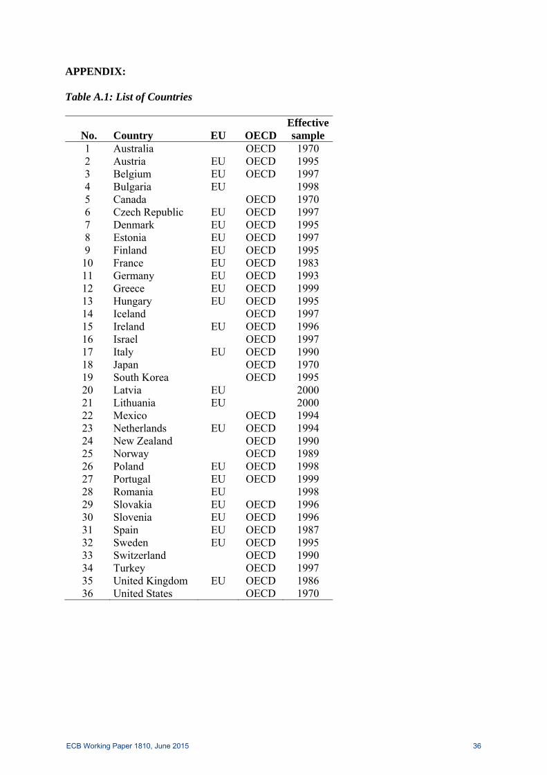
APPENDIX: Table A.1: List of Countries

No. Country EU OECD Effective sample

1 Australia OECD 1970 2 Austria EU OECD 1995 3 Belgium EU OECD 1997 4 Bulgaria EU 1998 5 Canada OECD 1970 6 Czech Republic EU OECD 1997 7 Denmark EU OECD 1995 8 Estonia EU OECD 1997 9 Finland EU OECD 1995 10 France EU OECD 1983 11 Germany EU OECD 1993 12 Greece EU OECD 1999 13 Hungary EU OECD 1995 14 Iceland OECD 1997 15 Ireland EU OECD 1996 16 Israel OECD 1997 17 Italy EU OECD 1990 18 Japan OECD 1970 19 South Korea OECD 1995 20 Latvia EU 2000 21 Lithuania EU 2000 22 Mexico OECD 1994 23 Netherlands EU OECD 1994 24 New Zealand OECD 1990 25 Norway OECD 1989 26 Poland EU OECD 1998 27 Portugal EU OECD 1999 28 Romania EU 1998 29 Slovakia EU OECD 1996 30 Slovenia EU OECD 1996 31 Spain EU OECD 1987 32 Sweden EU OECD 1995 33 Switzerland OECD 1990 34 Turkey OECD 1997 35 United Kingdom EU OECD 1986 36 United States OECD 1970


Table A.2: Common Sources and Definitions of Crises Banking Crises

No. Source Coverage and definitions 1.

Caprio and Klingebiel (2003)

The annual dataset (1970–2002) includes information on 117 episodes of systemic banking crises in 93 countries and on 51 episodes of borderline and non-systemic banking crises in 45 countries. A systemic crisis is defined as “much or all of bank capital was exhausted”. Expert judgment was also employed “for countries lacking data on the size of the capital losses, but also for countries where official estimates understate the problem”.

2.

Kaminsky and Reinhart (1999)

The monthly dataset (1970–1995) includes 26 episodes of banking crisis in 20 countries. Banking crises are defined by two types of events: “(1) bank runs that lead to the closure, merging, or takeover by the public sector of one or more financial institutions; and (2) if there are no runs, the closure, merging, takeover, or large-scale government assistance of an important financial institution (or group of institutions) that marks the start of a string of similar outcomes for other financial institutions”. The dataset of banking crises was compiled using existing studies of banking crises and the financial press.

3.

Laeven and Valencia (2008, 2010, 2012)

The annual dataset (1970–2011) covers systemically important banking crises (147 episodes) in over 100 countries all over the world and provides information on crisis management strategies. A banking crisis is considered to be systemic if the following two conditions are met: “(1) Significant signs of financial distress in the banking system (as indicated by significant bank runs, losses in the banking system, and/or bank liquidations); and (2) Significant banking policy intervention measures in response to significant losses in the banking system”. The first year that both criteria are met is considered to be the starting year of the banking crisis, and policy interventions in the banking sector are considered significant if at least three out of the following six measures were used: “(1) extensive liquidity support; (2) bank restructuring costs; (3) significant bank nationalizations; (4) significant guarantees put in place; (5) significant asset purchases; and (6) deposit freezes and bank holidays”. The dataset is compiled using the authors’ calculations combined with some elements of judgment for borderline cases.

4.

Reinhart and Rogoff (2008, 2011)

The annual dataset (1800–2010, from the year of independence) covers banking crises in 70 countries. The definition of banking crisis is the same as in Kaminsky and Reinhart (1999) (see above). The dataset of banking crises was compiled using existing studies of banking crises and the financial press.


Currency (Balance of Payment) Crises

No. Source Coverage and definitions 1. Kaminsky and

Reinhart (1999) The monthly dataset (1970–1995) includes 76 episodes of currency crisis in 20 countries. A currency crisis is defined as excessive exchange rate volatility (“turbulence”), that is, when the index representing a weighted average of changes in the exchange rate and reserves exceeds a certain threshold. “Crisis episodes” are then defined as “the month of the crisis plus the 24 months preceding the crisis”. For a robustness check, two alternative windows are used, starting at 12 and 18 months prior to the crisis. The dataset is compiled using the authors’ calculations.

2.

Kaminsky (2006)

The monthly dataset (1970–2002) includes 96 episodes of currency crisis in 20 industrial and developing countries. The definition of currency crises and “crisis episodes” is as in Kaminsky and Reinhart (1999). The dataset is compiled using the authors’ calculations.

3.

Laeven and Valencia (2008, 2010, 2012)

The annual dataset (1970–2011) includes 218 currency crises identified in over 100 countries all over the world. A currency crisis is defined as “a nominal depreciation of the currency vis-à-vis the U.S. dollar of at least 30 per cent that is also at least 10 percentage points higher than the rate of depreciation in the year before… For countries that meet the criteria for several continuous years, we use the first year of each 5-year window to identify the crisis.” It should be noted that this list also includes large devaluations by countries that adopt fixed exchange rate regimes.

2.

Reinhart and Rogoff (2011)

The annual dataset (1800–2010, from the year of independence) tracks currency crises (also called “crashes”) in 70 countries. A currency crisis is defined as an excessive exchange rate depreciation, that is, when the annual depreciation vis-à-vis USD or the relevant anchoring currency (GBP, FRF, DM, EUR) exceeds the threshold value of 15%. The dataset is compiled using the authors’ calculations.


Table A.3: Variables, Transformations and Data Sources

No. Variable Description Transform. Main source

Dependent binary variables of crisis onset (i)

banking

Banking crisis onset (1 if crisis was reported, 0 otherwise) as indicated by national central banks in survey run by authors

none

Authors’ compilation (see Babecký et al., 2012)

(ii)

currency

Currency crisis onset (1 if crisis was reported, 0 otherwise) as indicated by survey run by national central banks

none

Authors’ compilation (see Babecký et al., 2012)

Domestic macro and financial variables

1 curaccount Current account (% of GDP) none OECD, WDI

2 fx_reserves_growth FX reserves growth % yoy National central banks

3 gdpg Real GDP growth % yoy Statistical offices

4 govtbalance Government balance (% of GDP) none Statistical offices

5 govtdebt Government debt (% of GDP) none WDI, ECB

6 hhdebt Gross liabilities of personal sector growth % yoy National central banks, Oxford Economics

7 houseprices House price inflation % yoy BIS, Eurostat, Global Property Guide

8 hp_domprivcredit Domestic credit to private sector to GDP gap HP gap BIS, WDI

9 hp_neer Nominal effective exchange rate gap HP gap IFS

10 indprodch Industrial production growth % yoy Statistical offices

11 inflation Consumer price inflation % yoy Statistical offices, national central banks

12 m1 M1 growth % yoy National central banks

13 m3 M3 growth % yoy National central banks

14 nirspread Net interest rate spread (lending rate – deposit rate) none WDI

15 netsavings Net national savings (% of GNI) none WDI

16 shareprice Stock market index growth % yoy Reuters, stock exchanges

17 strate Short-term interest rate none IFS

18 termsoftrade Terms of trade change % yoy Statistical offices

19 unemployment Unemployment rate none Statistical offices

20

yieldcurve Yield curve slope (10Y government bond yield – money market interest rate)

none National central banks

Domestic structural variables

1

findev

Financial development

mean of 9 vars

WB – Global Fin. Dev. Database (variables: DI.01, DI.02, DI.04, DI.05, DI.06, DI.08, DI.12, SI.04, OI.02)

2

fxregime

De-facto exchange rate regime (discrete variable ranging from 1 – no sep. legal tender to 14 – free floating) none

Rose (2011) – online dataset on his website (variable: mcm_f_defacto)

3 indshare Industry share (% of GDP) none WDI, EIU

4 taxburden Total tax burden (% of GDP) none OECD, statistical offices

5 trade Trade (% of GDP) none WDI

International variables

1 baaspread BAA corporate bond spread none Reuters

2 comprice Commodity prices % yoy Commodity Research Bureau

3 hp_wcreditpriv Global domestic credit to private sector (% of GDP) HP gap WDI

4 wfdiinflow Global FDI inflow (% of GDP) none WDI

5 winf Global CPI inflation none IFS

6 wrgdp Global real GDP growth % yoy IFS

7 wtrade Global trade (constant prices) % yoy IFS


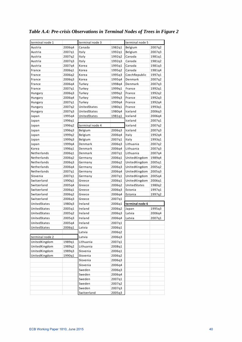
Table A.4: Pre-crisis Observations in Terminal Nodes of Trees in Figure 2

terminal node 1 terminal node 3 terminal node 5

Austria 2006q4 Canada 1982q1 Belgium 2007q2

Austria 2007q1 Italy 1992q1 Belgium 2007q3

Austria 2007q2 Italy 1992q2 Canada 1981q1

Austria 2007q3 Italy 1992q3 Canada 1981q2

Austria 2007q4 Korea 1995q1 Canada 1981q3

France 2006q1 Korea 1995q2 Canada 1981q4

France 2006q2 Korea 1995q3 CzechRepublic 1997q1

France 2006q3 Korea 1995q4 Denmark 2007q2

France 2006q4 Turkey 1998q4 Denmark 2007q3

France 2007q1 Turkey 1999q1 France 1992q1

Hungary 2006q3 Turkey 1999q2 France 1992q2



Hungary 2007q2 UnitedStates 1980q1 France 1993q1

Hungary 2007q3 UnitedStates 1980q4 Iceland 2006q3

Japan 1995q4 UnitedStates 1981q1 Iceland 2006q4

Japan 1996q1 Iceland 2007q1

Japan 1996q2 terminal node 4 Iceland 2007q2

Japan 1996q3 Belgium 2006q3 Iceland 2007q3

Japan 1999q2 Belgium 2006q4 Italy 1992q4

Japan 1999q3 Belgium 2007q1 Italy 1993q1

Japan 1999q4 Denmark 2006q3 Lithuania 2007q2

Korea 1996q1 Denmark 2006q4 Lithuania 2007q3

Netherlands 2006q1 Denmark 2007q1 Lithuania 2007q4

Netherlands 2006q2 Germany 2006q1 UnitedKingdom 1989q4




Slovenia 2007q1 Germany 2007q1 UnitedKingdom 2005q4

Switzerland 1990q1 Greece 2006q1 UnitedKingdom 2006q1

Switzerland 2005q4 Greece 2006q2 UnitedStates 1980q2

Switzerland 2006q1 Greece 2006q3 Estonia 1997q1

Switzerland 2006q2 Greece 2006q4 Estonia 1997q2

Switzerland 2006q3 Greece 2007q1

UnitedStates 1980q3 Ireland 2006q1 terminal node 6

UnitedStates 2005q1 Ireland 2006q2 Japan 1995q3

UnitedStates 2005q2 Ireland 2006q3 Latvia 2006q4

UnitedStates 2005q3 Ireland 2006q4 Latvia 2007q1

UnitedStates 2005q4 Ireland 2007q1

UnitedStates 2006q1 Latvia 2006q1

Latvia 2006q2

terminal node 2 Latvia 2006q3

UnitedKingdom 1989q1 Lithuania 2007q1

UnitedKingdom 1989q2 Lithuania 2008q1

UnitedKingdom 1989q3 Slovenia 2006q1

UnitedKingdom 1990q1 Slovenia 2006q2

Slovenia 2006q3

Slovenia 2006q4

Sweden 2006q3

Sweden 2006q4

Sweden 2007q1

Sweden 2007q2

Sweden 2007q3

Switzerland 2005q3


Table A.5: Pre-crisis Observations in Terminal Nodes of Trees in Figure 4 terminal node 2 terminal node 3

Iceland 2006q2 Iceland 2006q1

Iceland 2006q3 Iceland 2006q4

Turkey 1999q4 Iceland 2007q1

Italy 1991q1

Italy 1991q2

Italy 1991q3

Korea 1996q1

Korea 1996q2

Korea 1996q3

Korea 1996q4

Korea 1997q1

Spain 1990q3

Spain 1990q4

Spain 1991q1

Spain 1991q2

Spain 1991q3

Turkey 1999q1

Turkey 1999q2

Turkey 1999q3

Turkey 2000q1

UnitedKingdom 1990q4






Table A.6: Banking Crises within 4–8 Quarters – Logit Regression (Variables Pre-selected by RF, Pooled Sample)

Logistic regression Number of obs = 1861 LR chi2(10) = 79.73 Prob > chi2 = 0.0000 Log likelihood = -323.51113 Pseudo R2 = 0.1097 ---------------------------------------------------------------------------------- bank_w48 | Coef. Std. Err. z P>|z| [95% Conf. Interval] -----------------+---------------------------------------------------------------- curaccount | .1289704 .0308945 4.17 0.000 .0684184 .1895224 starate | -.0037019 .0412722 -0.09 0.929 -.084594 .0771902 yieldcurve | -.1825745 .0694474 -2.63 0.009 -.3186889 -.0464601 hp_domprivcredit | .0479306 .0111468 4.30 0.000 .0260832 .069778 govtbalance | -.0997083 .0332715 -3.00 0.003 -.1649193 -.0344974 m3 | .043914 .0241602 1.82 0.069 -.0034391 .0912671 unemployment | -.0921452 .0421866 -2.18 0.029 -.1748295 -.0094609 netsavings | -.0281272 .0156145 -1.80 0.072 -.058731 .0024767 govtdebt | -.0072376 .0045321 -1.60 0.110 -.0161204 .0016452 nirspread | -.1974979 .0510066 -3.87 0.000 -.2974689 -.0975268 constant | -1.347632 .5650595 -2.38 0.017 -2.455128 -.2401361 Notes: Variables in bold are those that appear in the baseline tree for banking crises (Figure 2)

Table A.7: Currency Crises within 4–8 Quarters – Logit Regression (Variables Pre-selected

by RF, Pooled Sample) Logistic regression Number of obs = 1996 LR chi2(10) = 92.80 Prob > chi2 = 0.0000 Log likelihood = -60.946463 Pseudo R2 = 0.4322 ---------------------------------------------------------------------------------- bop_w48 | Coef. Std. Err. z P>|z| [95% Conf. Interval] -----------------+---------------------------------------------------------------- hp_domprivcredit | .061257 .0243061 2.52 0.012 .0136178 .1088961 hp_neer | .3281974 .0583206 5.63 0.000 .2138911 .4425037 houseprices | -.0429796 .0363536 -1.18 0.237 -.1142314 .0282722 govtbalance | -.1917149 .0557448 -3.44 0.001 -.3009727 -.0824572 nirspread | .1612888 .0541118 2.98 0.003 .0552316 .267346 strate | .34505 .0954393 3.62 0.000 .1579924 .5321077 inflation | -.0921035 .0953281 -0.97 0.334 -.2789432 .0947361 curaccount | -.0335243 .0892786 -0.38 0.707 -.2085072 .1414586 unemployment | -.1623173 .1004662 -1.62 0.106 -.3592273 .0345928 indprodch | -.033967 .0518489 -0.66 0.512 -.135589 .067655 constant | -8.501559 1.017957 -8.35 0.000 -10.49672 -6.5064 ---------------------------------------------------------------------------------- Notes: Variables in bold are those that appear in the baseline tree for currency crises (Figure 5)


Acknowledgements

We devote this paper to the memory of Kateřina Šmídková, who started working on it but did not live to see its completion. We thank Tomáš Adam, Matthieu Bussiere, Sarah Holton, Glenn Hoggarth and Roman Horváth for their helpful comments. We thank the Global Property Guide (www.globalpropertyguide.com) for providing data on house prices. Rusnák acknowledges support from the Czech Science Foundation (Grant #P402/12/G097). The opinions expressed in this paper are solely those of the authors and do not necessarily reflect the views of the Bank of England or the Czech National Bank. Mark Joy

Bank of England, International Directorate, London, UK; e-mail: [email protected] Marek Rusnák

Czech National Bank, Financial Stability Department, Prague 1, Czech; e-mail: [email protected] Kateřina Šmídková

(in memoriam) Bořek Vašíček

Czech National Bank, Economic Research Department, Prague 1, Czech; e-mail: [email protected]

© European Central Bank, 2015

Postal address 60640 Frankfurt am Main, Germany Telephone +49 69 1344 0 Internet www.ecb.europa.eu All rights reserved. Any reproduction, publication and reprint in the form of a different publication, whether printed or produced electronically, in whole or in part, is permitted only with the explicit written authorisation of the ECB or the authors. This paper can be downloaded without charge from www.ecb.europa.eu, from the Social Science Research Network electronic library at http://ssrn.com or from RePEc: Research Papers in Economics at https://ideas.repec.org/s/ecb/ecbwps.html. Information on all of the papers published in the ECB Working Paper Series can be found on the ECB’s website, http://www.ecb.europa.eu/pub/scientific/wps/date/html/index.en.html. ISSN 1725-2806 (online) ISBN 978-92-899-1623-3 DOI 10.2866/748564 EU catalogue number QB-AR-15-050-EN-N

mailto:[email protected]



http://www.ecb.europa.eu/

http://www.ecb.europa.eu/

http://ssrn.com/

https://ideas.repec.org/s/ecb/ecbwps.html

http://www.ecb.europa.eu/pub/scientific/wps/date/html/index.en.html

banking and currency crises: differential diagnostics for

Documents