bandler, john w.; bakr, mohamed h.; rayas-sánchez, josé e. · j.w. bandler, m.h. bakr and j.e....

Instituto Tecnológico y de Estudios Superiores de Occidente

1999-06

Accelerated optimization of mixed EM/circuit

structures

Bandler, John W.; Bakr, Mohamed H.; Rayas-Sánchez, José E. Bandler, J.W; Bakr, M.H, and Rayas-Sánchez, J.E. (1999) “Accelerated optimization of mixed

EM/circuit structures,” in IEEE MTT-S Int. Microwave Symp. Workshop Notes and Short Courses,

Anaheim, CA, Jun.

Enlace directo al documento: http://hdl.handle.net/11117/1407

Este documento obtenido del Repositorio Institucional del Instituto Tecnológico y de Estudios Superiores de

Occidente se pone a disposición general bajo los términos y condiciones de la siguiente licencia:

http://quijote.biblio.iteso.mx/licencias/CC-BY-NC-ND-2.5-MX.pdf

(El documento empieza en la siguiente página)

Repositorio Institucional del ITESO rei.iteso.mx

Departamento de Electrónica, Sistemas e Informática DESI - Artículos y ponencias con arbitraje

http://www.iteso.mx

http://rei.iteso.mx

http://hdl.handle.net/11117/1407

http://quijote.biblio.iteso.mx/licencias/CC-BY-NC-ND-2.5-MX.pdf

ACCELERATED OPTIMIZATION OF MIXED EM/CIRCUIT STRUCTURES

J.W. Bandler, M.H. Bakr and J.E. Rayas-Sánchez

SOS-99-8-V

March 1999

J.W. Bandler, M.H. Bakr and J.E. Rayas-Sánchez 1999 No part of this document may be copied, translated, transcribed or entered in any form into any machine without written permission. Address enquiries in this regard to Dr. J.W. Bandler. Excerpts may be quoted for scholarly purposes with full acknowledgement of source. This document may not be lent or circulated without this title page and its original cover.



Simulation Optimization Systems Research Laboratory and Department of Electrical and Computer Engineering McMaster University, Hamilton, Canada L8S 4K1

[email protected] www.sos.mcmaster.ca

presented at

WORKSHOP ON ADVANCES IN MIXED ELECTROMAGNETIC FIELD AND CIRCUIT SIMULATION

1999 IEEE MTT-S Int. Microwave Symposium, Anaheim, CA, June 18, 1999

Simulation Optimization Systems Research LaboratoryMcMaster University

99-8-2



Simulation Optimization Systems Research Laboratory and Department of Electrical and Computer Engineering McMaster University, Hamilton, Canada L8S 4K1

[email protected] www.sos.mcmaster.ca

Abstract We review recent developments in Space Mapping (SM) optimization. The Aggressive Space Mapping (ASM) technique is illustrated through a step-by-step numerical example based on the Rosenbrock function. The Trust Region Aggressive Space Mapping (TRASM) algorithm is described. TRASM integrates a trust region methodology with the ASM technique. It improves the uniqueness of the extraction phase by utilizing a recursive multi-point parameter extraction process. The algorithm is illustrated by the design of an HTS filter using Sonnet’s em. The new Hybrid Aggressive Space Mapping (HASM) algorithm is briefly reviewed. It is based on a novel lemma that enables smooth switching from SM optimization to direct optimization if SM is not converging. It is illustrated by the design of a six-section H-plane waveguide filter.


99-8-3

Basic Concepts of Space Mapping (Bandler et al., 1993, 1994) it is assumed that the circuit to be designed can be simulated using two models: a “fine” model and a “coarse” model

the fine model is accurate but computationally intensive x f is the vector of fine model design parameters the coarse model is fast but less accurate xc is the vector of coarse model design parameters Space Mapping aims at avoiding the computationally intensive direct optimization of the fine model by iteratively developing a mapping between x f and xc we present illustrations and progress to date on this exciting concept applied to accelerated optimization of mixed EM/circuit structures


99-8-4

Aggressive Space Mapping (ASM) Concept

fx )( ff xRfine

modelcoarsemodel

cx )( cc xR

Start

Choose the coarse optimalsolution as a starting point

for the fine model

x xf c *

Calculate the fineresponse

R xf f

PARAMETER EXTRACTION:Find the optimal value of

such that

COARSE OPTIMIZATION:Find the optimal response using

the coarse model

R xc c*

R x R xc c f f

xc

End

?

x xc c *

yes

Update

using Broyden's formula

no

x f


99-8-5

An Aggressive Space Mapping (ASM) Algorithm (Bandler et al., 1995) the initial fine model design is taken as x*

c

at the jth iteration

hxx )()()1( jjf

jf

h )( j is obtained by solving

)( )()()( xfhBj

fjj

where xxf *)(

cj

c and x )( j

c is obtained through parameter extraction

xf,1

xf,2

xc,1

xc,2

x*c

xc(1)

x )1(f

x )2(f


99-8-6

ASM Algorithm

Step 0. Initialize *)1(cf xx , 1B )1( , 1j .

Step 1. Evaluate )( )1(ff xR .

Step 2. Extract )1(cx such that )()( )1()1(

ffcc xRxR .

Step 3. Evaluate *)1()1(cc xxf . Stop if )1(f .

Step 4. Solve )()()( jjj fhB for )( jh .

Step 5. Set )()()1( jjf

jf hxx .

Step 6. Evaluate )( )1( jff xR .

Step 7. Extract )1( jcx such that )()( )1()1( j

ffj

cc xRxR .

Step 8. Evaluate *)1()1(c

jc

j xxf . Stop if )1( jf .

Step 9. Update )()(

)()1()()1(

jTj

Tjjjj

hh

hfBB

.

Step 10. Set 1 jj ; go to Step 4.


99-8-7

Parameter Extraction single point parameter extraction aims at matching the responses of both models at a single point

it can be formulated as

)()( xRxRx

ccff

c

minimize

multi-point parameter extraction aims at simultaneously matching the responses at a number of corresponding points

the extracted parameters should satisfy

)())(( xRxxBxR ffcc

simultaneously for a set of points Vx

xf,1

xf,2

xc,1

xc,2

Rc Rf

xf

xc

xf,1

xf,2

xc,1

xc,2

xf

V xc

B


99-8-8

Coarse Model Example: Rosenbrock Function

21

2212 )1()(100)( xxxRc x , where

2

1

x

xx

-2 -1.5 -1 -0.5 0 0.5 1 1.5 2-1

-0.5

0

0.5

1

1.5

2

2.5

3

X1

X2

Coarse response, Rc

1

1*cx

0)( ** ccc RR x


99-8-9

Fine Model : Shifted Rosenbrock Function 2

122

12 )1()(100)( uuuR f x where

2.0

2.0

2

1 xuu

u

-2 -1.5 -1 -0.5 0 0.5 1 1.5 2-1

-0.5

0

0.5

1

1.5

2

2.5

3

X1

X2

Fine response, Rf

P1

P2

P3

P4

P5


99-8-10

Multi-Point Parameter Extraction we minimize a parameter extraction objective function

pE

considering five matching points, with error functions

)Δ()Δ( *)(icfi

jci RRE xxxBx

where

0

01x ,

5.0

02x ,

0

5.03x ,

5.0

5.04x ,

5.0

5.05x

since the matrix 1B )( j for the first parameter extraction optimization, the corresponding five error functions are taken as

)Δ()Δ( *icfici RRE xxxx

considering only 1l and 2l norms, the corresponding objective functions can be taken as

nn EEEABS 21 22

22

1 )()()( nn EEESQR


99-8-11

l1 Objective Function for the Parameter Extraction Problem

0.4 0.5 0.6 0.7 0.8 0.9 1 1.1 1.2 1.3 1.40.8

0.9

1

1.1

1.2

1.3

X1

X2Absolute value of error 1, ABS1

single point parameter extraction

0.4 0.5 0.6 0.7 0.8 0.9 1 1.1 1.2 1.3 1.40.8

0.9

1

1.1

1.2

1.3

X1

X2

Absolute value of errors 1, 2, 3, 4 and 5: ABS5

2.1

8.0)1(cx

multi-point parameter extraction (with 4 additional points)


99-8-12

l2 Objective Function for the Parameter Extraction Problem

0.4 0.5 0.6 0.7 0.8 0.9 1 1.1 1.2 1.3 1.40.8

0.9

1

1.1

1.2

1.3

X1

X2

Square of error 1, SQR1


0.4 0.5 0.6 0.7 0.8 0.9 1 1.1 1.2 1.3 1.40.8

0.9

1

1.1

1.2

1.3

X1

X2

Square of errors 1, 2, 3, 4 and 5: SQR5

2.1

8.0)1(cx



99-8-13

Space Mapping Solution Process

Step 0.

1

1)1(fx , 1B )1( , 1j

Step 1. 4.31)( )1( ffR x

Step 2. When

2.1

8.0)1(cx , )()( )1()1(

ffcc RR xx

Step 3.

2.0

2.0

1

1

2.1

8.0)1(f

Step 4. Since 1B )1( ,

2.0

2.0)1(h

Step 5. Set

8.0

2.1

2.0

2.0

1

1)2(fx

Step 6. 0)( )2( ffR x

Step 7.

1

1)2(cx , because we know 0)( )2( ccR x

Step 8. Since

0

0*)2()2(cc xxf , then

8.0

2.1)2(ff xx


99-8-14

Fine Model Example: Transformed Rosenbrock Function 2

122

12 )1()(100)( uuuR f x where

3.0

3.0

9.02.0

2.01.1

2

1 xuu

u

-2 -1.5 -1 -0.5 0 0.5 1 1.5 2-1

-0.5

0

0.5

1

1.5

2

2.5

3

X1

X2

Fine response, Rf

32.108)( * cf xR


99-8-15

First l1 Parameter Extraction

-1.5 -1 -0.5 0 0.5 1 1.5 2-1

-0.5

0

0.5

1

1.5

2

X1

X2

Absolute value of error 1, ABS1


-1.5 -1 -0.5 0 0.5 1 1.5 2-1

-0.5

0

0.5

1

1.5

2

X1

X2

Absolute value of errors 1, 2 and 3: ABS3

4.1

6.0)1(cx



99-8-16

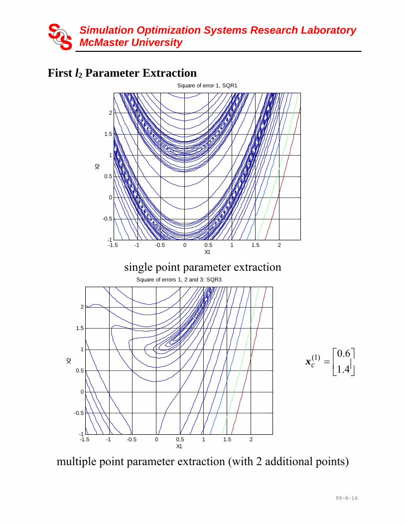
First l2 Parameter Extraction

-1.5 -1 -0.5 0 0.5 1 1.5 2-1

-0.5

0

0.5

1

1.5

2

X1

X2



-1.5 -1 -0.5 0 0.5 1 1.5 2-1

-0.5

0

0.5

1

1.5

2

X1

X2

Square of errors 1, 2 and 3: SQR3

4.1

6.0)1(cx

multiple point parameter extraction (with 2 additional points)


99-8-17

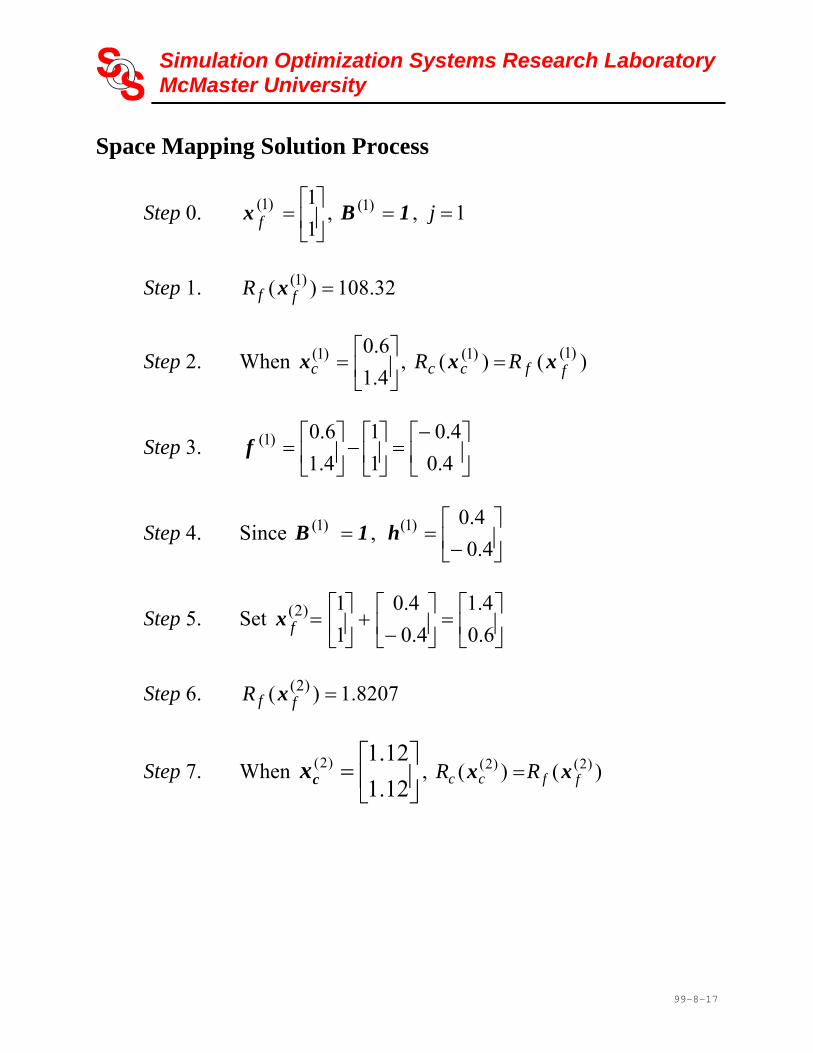
Space Mapping Solution Process

Step 0.

1

1)1(fx , 1B )1( , 1j

Step 1. 32.108)( )1( ffR x

Step 2. When

4.1

6.0)1(cx , )()( )1()1(

ffcc RR xx

Step 3.

4.0

4.0

1

1

4.1

6.0)1(f

Step 4. Since 1B )1( ,

4.0

4.0)1(h

Step 5. Set

6.0

4.1

4.0

4.0

1

1)2(fx

Step 6. 8207.1)( )2( ffR x

Step 7. When

12.1

12.1)2(cx , )()( )2()2(

ffcc RR xx


99-8-18

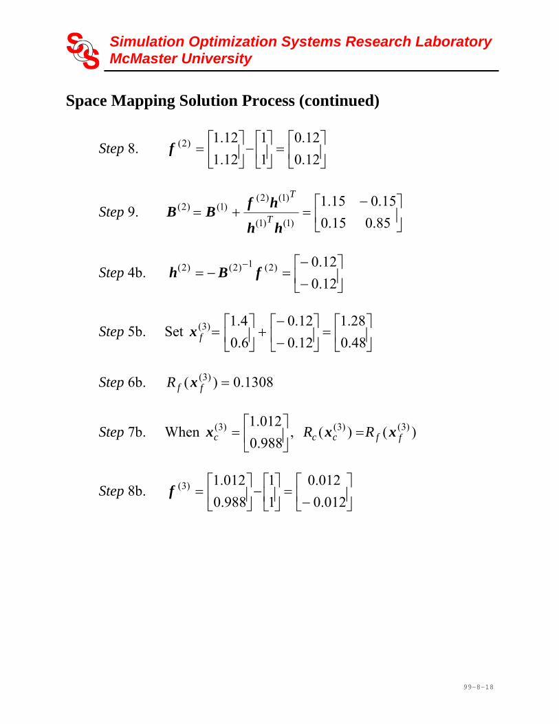
Space Mapping Solution Process (continued)

Step 8.

12.0

12.0

1

1

12.1

12.1)2(f

Step 9.

85.015.0

15.015.1

)1()1(

)1()2()1()2(

hh

hfBB

T

T

Step 4b.

12.0

12.0)2(1)2()2( fBh

Step 5b. Set

48.0

28.1

12.0

12.0

6.0

4.1)3(fx

Step 6b. 1308.0)( )3( ffR x

Step 7b. When

988.0

012.1)3(cx , )()( )3()3(

ffcc RR xx

Step 8b.

012.0

012.0

1

1

988.0

012.1)3(f


99-8-19

Space Mapping Solution Process (continued)

Step 9b.

9.02.0

2.01.1

)2()2(

)2()3()2()3(

hh

hfBB

T

T

Step 4c.

0151.0

0082.0)3(1)3()3( fBh

Step 5c. Set

4951.0

2718.1

0151.0

0082.0

48.0

28.1)4(fx

Step 6c. 8)4( 102.9)( ff xR , then )4(ff xx and we can

end the algorithm


99-8-20

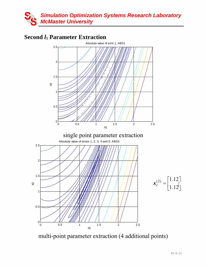
Second l1 Parameter Extraction

0 0.5 1 1.5 2 2.50

0.5

1

1.5

2

2.5

X1

X2



0 0.5 1 1.5 2 2.50

0.5

1

1.5

2

2.5

X1

X2

Absolute value of errors 1, 2, 3, 4 and 5: ABS5

12.1

12.1)2(cx

multi-point parameter extraction (4 additional points)


99-8-21

Second l2 Parameter Extraction

0 0.5 1 1.5 2 2.50

0.5

1

1.5

2

2.5

X1

X2



0 0.5 1 1.5 2 2.50

0.5

1

1.5

2

2.5

X1

X2

Square of errors 1, 2, 3, 4 and 5: SQR5

12.1

12.1)2(cx



99-8-22

Third Parameter Extraction

-0.5 0 0.5 1 1.5 2 2.5-0.5

0

0.5

1

1.5

2

2.5

X1

X2


988.0

012.1)3(cx

single point l1 parameter extraction

-0.5 0 0.5 1 1.5 2 2.5-0.5

0

0.5

1

1.5

2

2.5

X1

X2


988.0

012.1)3(cx

single point l2 parameter extraction


99-8-23

The Trust Region Aggressive Space Mapping (TRASM) Algorithm (Bakr et al., 1998)

TRASM integrates a trust region methodology with ASM a certain success criterion must be satisfied in each iteration to accept the predicted step a recursive multi-point parameter extraction procedure is introduced all available fine model simulations are utilized to improve parameter extraction uniqueness available mapping information is integrated into this extraction procedure


99-8-24

Illustration of the TRASM Algorithm

xc,1

xc,2

xf,1

xf,2

x )(if

the current state at the ith iteration

trust region

)( )(xP if

initial parameter extraction at the suggested point

xc,1

xc,2

xf,1

xf,2

)( )1(xP if

x )(if

x 1)( if

trust region

xc,1

xc,2

)( )1(xP if

xf,1

xf,2

x )(if

x 1)( if

x 1t

multi-point extraction is applied


99-8-25

TRASM Algorithm (Bakr et al., 1998) using xxPf *)()( )( c

if

i

solve ( )( ) ( ) ( ) ( )( )ii T i i T i B B I h B f for

( )ih

this corresponds to minimizing 2

2( ) ( ) ( )i i if B h subject to

2( )ih where is the size of the trust region

, which correlates to , can be determined (Moré et al., 1983) single point parameter extraction is performed at the new point

hxx )()(1)( iif

if to get ( 1)if

if ( 1)if satisfies a certain success criterion for the reduction in

the l2 norm of the vector f, the point x 1)( if is accepted and the

matrix ( )iB is updated using Broyden’s update otherwise a temporary point is generated using x 1)( i

f and ( 1)if

and is added to the set of points to be used for multi-point parameter extraction a new ( 1)if is obtained through multi-point parameter extraction


99-8-26

TRASM Algorithm (continued) the last three steps are repeated until a success criterion is satisfied or the step is declared a failure step failure has two forms (1) f may approach a limiting value without satisfying the

success criterion or (2) the number of fine model points simulated since the

last successful step reaches n+1 Case (1): the parameter extraction is trusted but the linearization used is suspect; the size of the trust region is decreased and a new point x 1)( i

f is obtained

Case (2): sufficient information is available for an approximation to the Jacobian of the fine model responses w.r.t. the fine model parameters used to predict the new point x 1)( i

f

the mapping between the two spaces is exploited in the parameter extraction step by solving

))())(( )1()( xRxxBxRx

fif

icc

c

minimize

simultaneously for a set of points x


99-8-27

The Current Implementation the algorithm is currently implemented in MATLAB OSA90 is used as a platform for the multi-point parameter extraction and for the fine model simulations

TRASM: Trust Region Aggressive Space Mapping

TRASM

Algorithm (MATLAB)

Parameters

Responses

OSA90

Responses

HP HFSS

Sonnet’s em

Empirical Models

Extracted Parameters

Parameter Extraction

Fine Model Simulation


99-8-28

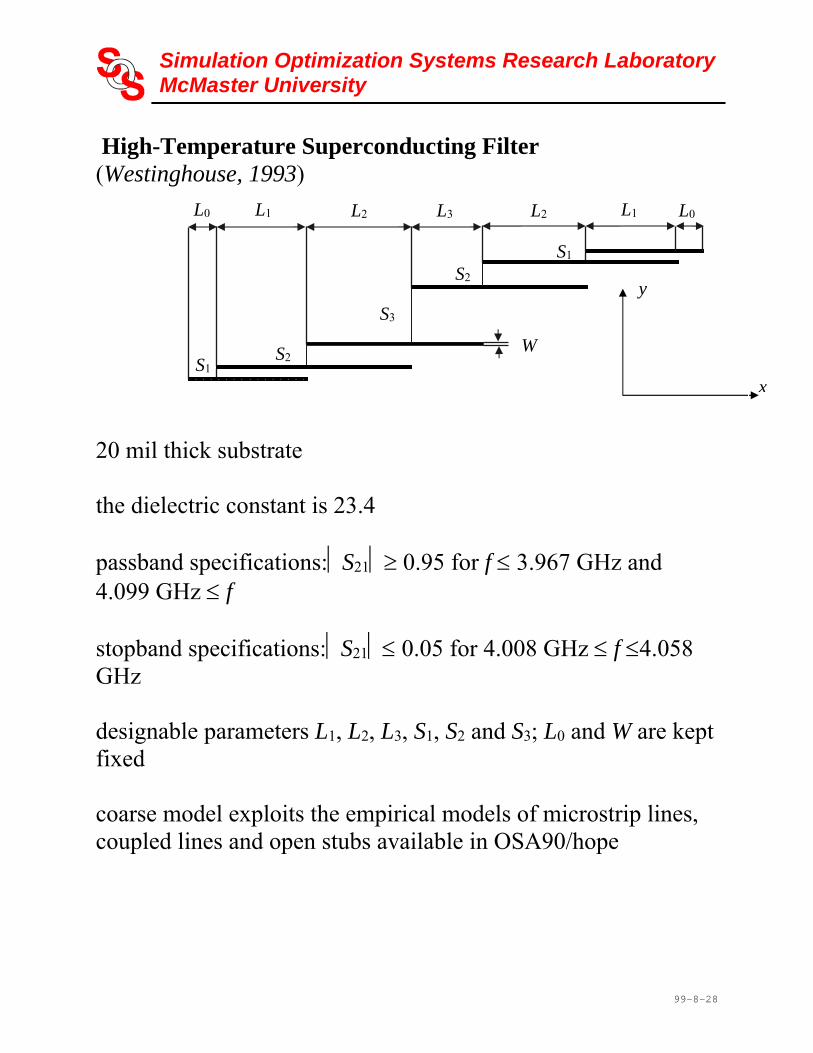
High-Temperature Superconducting Filter (Westinghouse, 1993)

20 mil thick substrate the dielectric constant is 23.4 passband specifications:S21 0.95 for f 3.967 GHz and 4.099 GHz f stopband specifications:S21 0.05 for 4.008 GHz f 4.058 GHz designable parameters L1, L2, L3, S1, S2 and S3; L0 and W are kept fixed coarse model exploits the empirical models of microstrip lines, coupled lines and open stubs available in OSA90/hope

L0 L1 L2 L3 L2 L1 L0

S1

S2

S3

S2 S1

W

x

y


99-8-29

High-Temperature Superconducting Filter Fine Model the fine model employs a fine-grid Sonnet em simulation the x and y grid sizes for em are 1.0 and 1.75 mil 100 elapsed minutes are needed for em analysis at single frequency on a Sun SPARCstation 10 final design is obtained in 5 TRASM iterations, requiring 8 em simulations 15 frequency points are used per em simulation


99-8-30

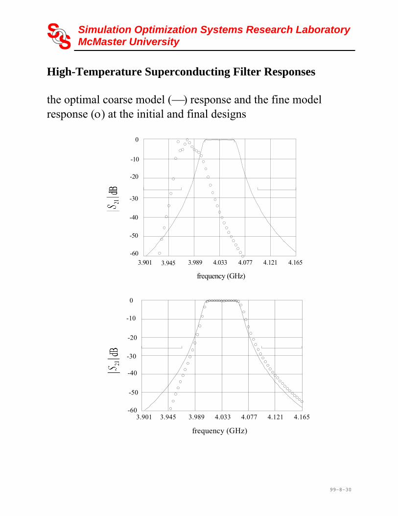
High-Temperature Superconducting Filter Responses the optimal coarse model () response and the fine model response () at the initial and final designs

3.901 3.945 3.989 4.033 4.077 4.121 4.165

frequency (GHz)

-60

-50

-40

-30

-20

-10

0

3.901 3.945 3.989 4.033 4.077 4.121 4.165

frequency (GHz)

-60

-50

-40

-30

-20

-10

0


99-8-31

Passband Details for the High-Temperature Superconducting Filter

3.967 3.989 4.011 4.033 4.055 4.077 4.099

frequency (GHz)

-1.50

-1.25

-1.00

-0.75

-0.50

-0.25

0


99-8-32

Motivation for a Hybrid Algorithm the TRASM algorithm is efficient the number of fine model simulations needed is of the order of the problem dimension any SM algorithm assumes the existence of a coarse model which is fast and has sufficient accuracy if the coarse model is severely misaligned from the fine model SM optimization may not converge the solution obtained using TRASM for most problems is a near an optimal solution however, optimality can not be guaranteed as the optimal coarse model may significantly deviate from the optimal fine model


99-8-33

Illustrative Example: A Rosenbrock Function consider a coarse model as

)1()(100 122

122

xxx Rc

and a fine model as

))(1())()((100 112

112

22

2 xxx R f

where 1 and 2 are constant shifts suppose the target of the direct optimization problem is to minimize Rf

the optimal coarse model design is x*

c =[1.0 1.0]T

the optimal fine model design is x*

f =[(11) (1 2 )]T

the misalignment between the two models is thus given by the two shifts 1 and 2


99-8-34

Illustrative Example: A Rosenbrock Function consider the case 1= 2=0.1

ideal contour plot of xxP * 2

2)( cf

actual contour plot of xxP * 2

2)( cf

the TRASM algorithm is likely to converge

x1

-1.0 -0.5 0 0.5 1.0 1.5 2.0 2.5 3.00

0.5

1.0

1.5

2.0

2.5

3.0

x 2

x1 -1.0 -0.5 0 0.5 1.0 1.5 2.0 2.5 3.0

0

0.5

1.0

1.5

2.0

2.5

3.0

x2


99-8-35

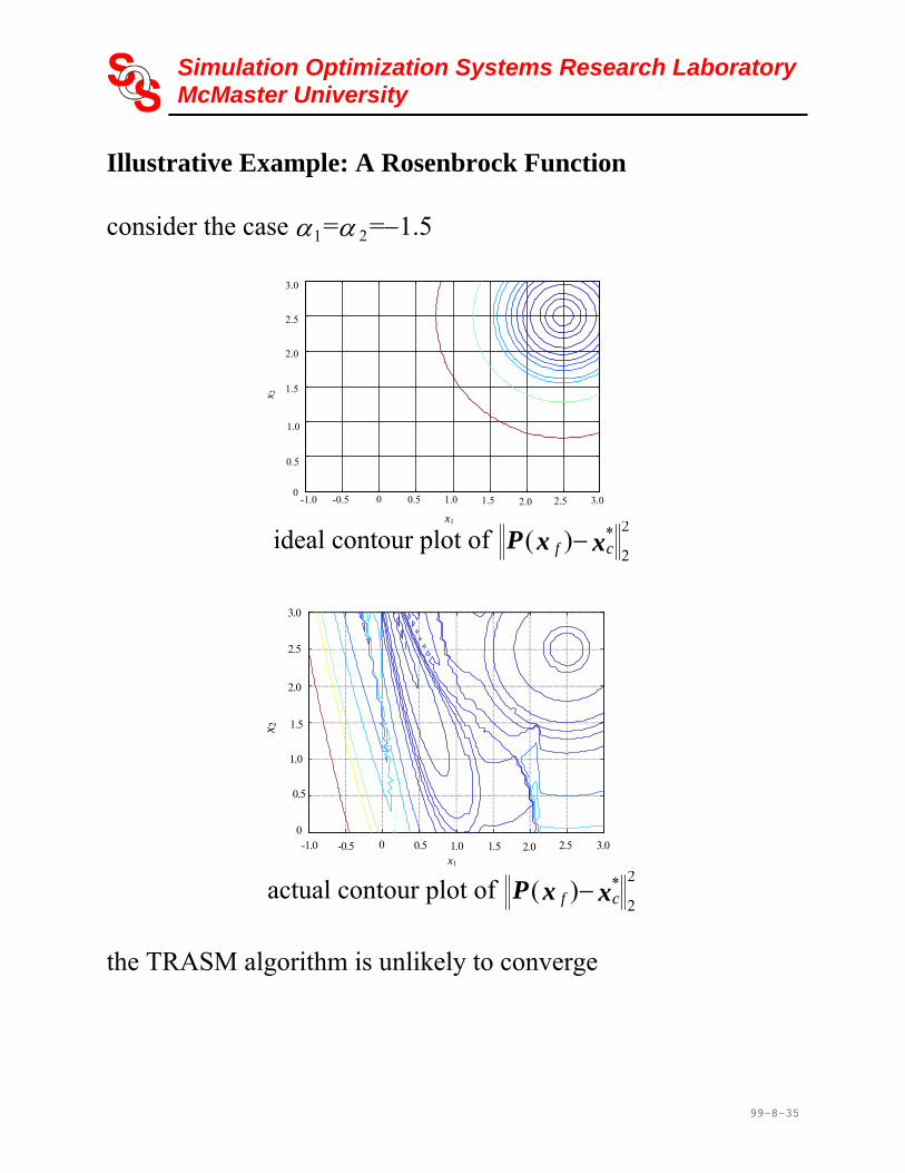
Illustrative Example: A Rosenbrock Function consider the case 1= 2=1.5

ideal contour plot of xxP * 2

2)( cf

actual contour plot of xxP * 2

2)( cf

the TRASM algorithm is unlikely to converge

x1

-1.0 -0.5 0 0.5 1.0 1.5 2.0 2.5 3.00

0.5

1.0

1.5

2.0

2.5

3.0 x 2

-1.0 -0.5 0 0.5 1.0 1.5 2.0 2.5 3.00

0.5

1.0

1.5

2.0

2.5

3.0

x 2

x1


99-8-36

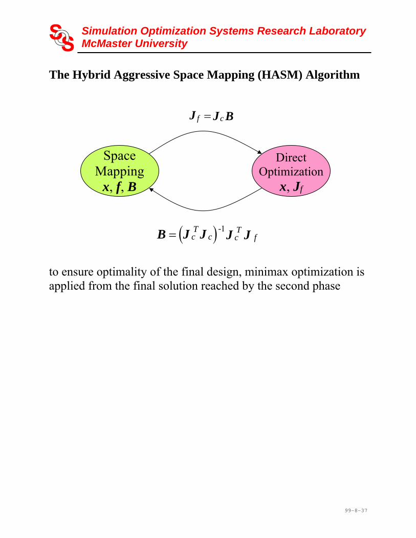
The Hybrid Aggressive Space Mapping (HASM) Algorithm (Bakr et al., 1999) the HASM algorithm is designed to handle severely misaligned cases it utilizes two different phases the first phase utilizes the TRASM algorithm if the TRASM algorithm is not converging smoothly a switch takes place to the second phase this switch utilizes mapping information to supply a Jacobian estimate for the fine model response to the second phase the second phase applies direct optimization to match the fine model response to the optimal coarse model response a switch back to the first phase can take place if SM convergence is potentially smooth the Jacobian of the fine model response and parameter extraction are then utilized to recover the mapping matrix B several switches can take place between the two phases


99-8-37

The Hybrid Aggressive Space Mapping (HASM) Algorithm to ensure optimality of the final design, minimax optimization is applied from the final solution reached by the second phase

Space Mapping

x, f, B

Direct Optimization

x, Jf

JJJJB fT cc

T c

- 1

BJJ cf


99-8-38

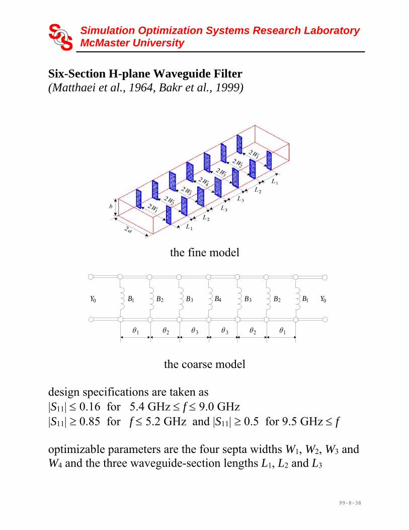
Six-Section H-plane Waveguide Filter (Matthaei et al., 1964, Bakr et al., 1999)

the fine model

the coarse model

design specifications are taken as |S11| 0.16 for 5.4 GHz f 9.0 GHz |S11| 0.85 for f 5.2 GHz and |S11| 0.5 for 9.5 GHz f optimizable parameters are the four septa widths W1, W2, W3 and W4 and the three waveguide-section lengths L1, L2 and L3

Y0 2B1B 3B 4B 3B 2B 1B Y0

1 12 2 3 3


99-8-39

Six-Section H-plane Waveguide Filter the coarse model consists of lumped inductances and dispersive transmission line sections

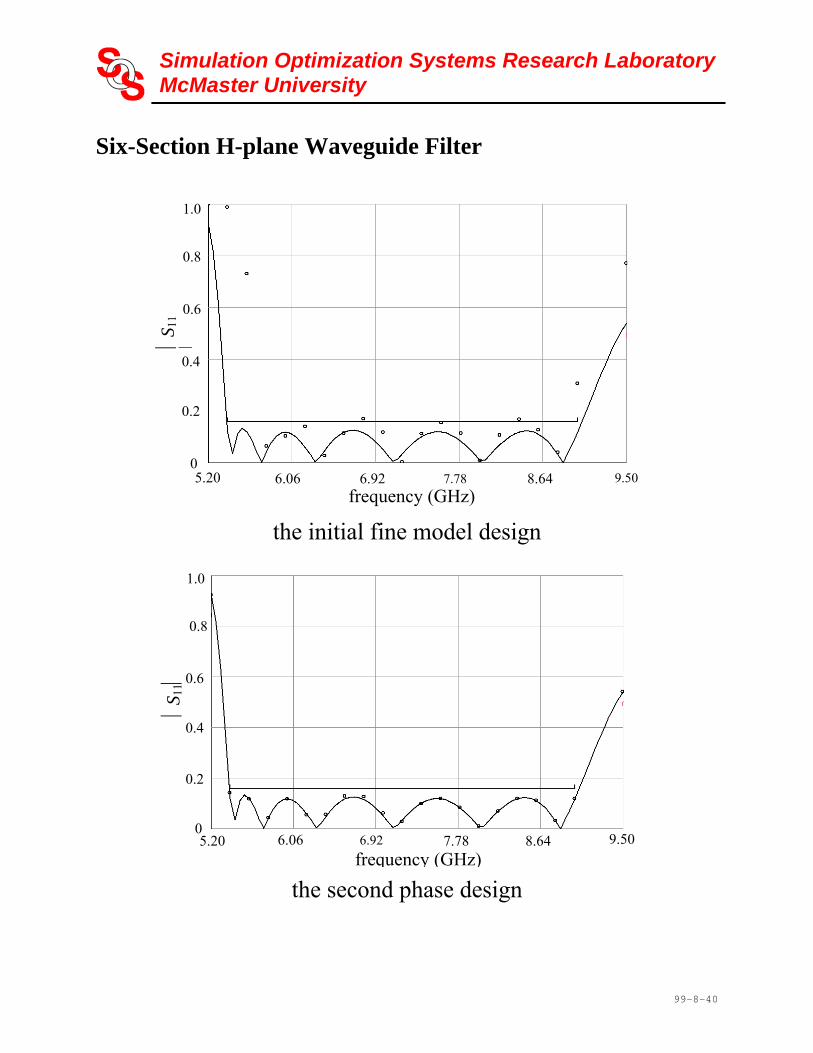
a simplified version of a formula (Marcuvitz, 1951) is utilized in evaluating the inductances the fine model exploits HP HFSS through HP Empipe3D the first phase executed 4 iterations requiring a total of 5 fine model simulations the second phase did not produce successful iterations the optimal fine model design is obtained using minimax optimization the convergence of TRASM is smooth: the fine model response at the end of the first phase is almost identical to the optimal fine model response


99-8-40

Six-Section H-plane Waveguide Filter

the initial fine model design

the second phase design

5.20 6.06 6.92 7.78 8.64 9.50

frequency (GHz)

0

0.2

0.4

0.6

0.8

1.0

S11

5.20 6.06 6.92 7.78 8.64 9.50 0

0.2

0.4

0.6

0.8

1.0

frequency (GHz)

S11


99-8-41

Six-Section H-plane Waveguide Filter

the optimal fine model design

5.20 6.06 6.92 7.78 8.64 9.50

frequency (GHz)

0

0.2

0.4

0.6

0.8

1.0

S11


99-8-42

References J.W. Bandler, R.M. Biernacki, S.H. Chen, P.A. Grobelny and R.H. Hemmers, “Space mapping technique for electromagnetic optimization,” IEEE Trans. Microwave Theory Tech., vol. 42, 1994, pp. 2536-2544. J.W. Bandler, R.M. Biernacki, S.H. Chen, R.H. Hemmers and K. Madsen, “Electromagnetic optimization exploiting aggressive space mapping,” IEEE Trans. Microwave Theory Tech., vol. 43, 1995, pp. 2874-2882. J.W. Bandler, R.M. Biernacki and S.H. Chen, “Fully automated space mapping optimization of 3D structures,” IEEE MTT-S Int. Microwave Symp. Dig. (San Francisco, CA), 1996, pp. 753-756. M.H. Bakr, J.W. Bandler, R.M. Biernacki, S.H. Chen and K. Madsen, “A trust region aggressive space mapping algorithm for EM optimization,” IEEE Trans. Microwave Theory Tech., vol. 46, 1998, pp. 2412-2425. J.J. Moré and D.C. Sorenson, “Computing a trust region step,” SIAM J. Sci. Stat. Comp., vol. 4, 1983, pp. 553-572. C.G. Broyden, “A class of methods for solving nonlinear simultaneous equations,” Math. Comp., vol. 19, 1965, pp. 577-593. J.W. Bandler, R.M. Biernacki, S.H. Chen, W.J. Gestinger, P.A. Grobelny, C. Moskowitz and S.H. Talisa, “Electromagnetic design of high-temperature superconducting filters,” Int. J. Microwave and Millimeter-Wave CAE, vol. 5, 1995, pp. 331-343. em, Sonnet Software, Inc., 1020 Seventh North Street, Suite 210, Liverpool, NY 13088, 1997. M.H. Bakr, J.W. Bandler, N. Georgieva and K. Madsen, “A hybrid aggressive space mapping algorithm for EM optimization,” IEEE MTT-S Int. Microwave Symp. (Anaheim, CA), June 1999. G.L. Matthaei, L. Young and E.M. T. Jones, Microwave Filters, Impedance-Matching Network and Coupling Structures. New York: McGraw-Hill, First Edition, 1964. N. Marcuvitz, Waveguide Handbook. New York: McGraw-Hill, First Edition, 1951, p. 221. HP HFSS Version 5.2, HP EEsof Division, 1400 Fountaingrove Parkway, Santa Rosa, CA 95403-1799, 1998. HP Empipe3D Version 5.2, HP EEsof Division, 1400 Fountaingrove Parkway, Santa Rosa, CA 95403-1799, 1998.

bandler, john w.; bakr, mohamed h.; rayas-sánchez, josé e. · j.w. bandler, m.h. bakr and j.e....

Documents