Balanced-Budget Rules, Energy Taxes, and Aggregate Instability�

YAN ZHANG

Shanghai Jiao-Tong University

�This is a shortened version of my dissertation at New York University, "Tari¤ and Equilibrium Indeterminacy".I would like to thank my advisers, Jess Benhabib and Jushan Bai, for their guidance. I likewise thank Luis Aguiar-Conraria, Pierpaolo Benigno, Yan Chen, Paul Dower, Jang-Ting Guo, Boyan Jovanovic, Lu Lei, Viktor Tsyrennikov,Martin Uribe, Alain Venditti, Yi Wen, Vivian Yue, Lin Zhou and seminar participants at the 8th Journees Louis-AndreGerard-Varet conference in public economics held in Marseille in June 2009 for their valuable comments. Finally, Iacknowledge the �nancial support of New York University (Henry M. MacCracken Fellowship) and Shanghai JiaoTong University. Address correspondence to Zhang Yan, Department of Economics, Antai College of Economics andManagement, Shanghai Jiao Tong University, Shanghai, 200052, China. Tel: 86-21-52302560; E-mail address:zhangyan77@sjtu.edu.cn.

1

Author: YAN ZHANG

Running head: BALANCED-BUDGET RULES, ENERGY TAXES, AND AGGREGATE INSTA-

BILITY

Abstract: We study the e¤ect of energy taxes (or tari¤s), using a standard neoclassical growth model

with imported energy for production. We �nd that (1) the model may exhibit local indeterminacy

and sunspots when energy tax rates are endogenously determined by a balanced-budget rule, with a

constant level of government expenditures (or lump-sum tansfer); and (2) indeterminacy disappears

if the government �nances endogenous public spending and transfers with �xed tax rates. Under

the �rst type of balanced budget formulation, we provide calibration examples to illustrate that

endogenous energy taxes can easily make an otherwise determinate economy indeterminate. Under

the second type of balanced-budget formulation, we prove that the economy exhibits equilibrium

uniqueness regardless of the existence of lump-sum transfers. In addition, analyses show that without

variable capacity utilization, local indeterminacy cannot occur for empirically plausible values of

energy tax rates.

JEL: E32, E62.

Keywords: Indeterminacy, Endogenous energy tax rate, Balanced-budget rule.

2

1. INTRODUCTION

Numerous studies on trade taxes have recently suggested that a government can rely heavily on energy

taxes (or tari¤s) for its revenues. Although many previous works focused on cases of determinacy in

dynamic stochastic general equilibrium (DSGE) models with energy for production [Rotemberg and

Woodford (1994); de Miguel and Manzano (2006)], energy taxes on intermediate goods (e.g., imported

energy), which act like taxes on returns to factors of production, may generate local indeterminacy

in a way that is similar to factor income taxes.

The pioneering work of Schmitt-Grohe and Uribe (1997; henceforth SGU) shows that, in a neo-

classical growth model with a pre-set level of government expenditures (or lump-sum transfers), if

the labor income tax rates are endogenously determined by a balanced-budget rule, the model can

exhibit local indeterminacy for empirically plausible values of income tax rates. Guo and Harrison

(2004; henceforth GH) further show that constant income tax rates cannot be a source of local

indeterminacy per se in a neoclassical growth model.

In this paper, we extend the above-mentioned analyses by studying the role of public spending

�nanced by energy taxes (or tari¤s) in the emergence of local indeterminacy, and do so within a stan-

dard neoclassical growth model with energy for production-for the same class of �scal policy rules.1

We �nd that energy and labor income taxes can generate local indeterminacy in a similar manner

when �scal increasing returns arise. More precisely, we consider a countercyclical energy tax policy,

in which constant government expenditures (or lump-sum transfers) are �nanced by endogenous tax

rates. In addition, we consider a �at energy tax policy, in which endogenous government expenditures

(or lump-sum transfers) are �nanced by constant tax rates. We �nd that a countercyclical energy

tax policy is required in generating local indeterminacy, whereas a �at energy tax policy causes the

1For simplicity, we assume that the government does not impose consumption taxes on the tradable goods or factorincome taxes on the production factors.

3

economy to be immune to local indeterminacy regardless of the existence of lump-sum transfers.

Under the balanced-budget rule with a countercyclical tax policy, we provide calibration examples

for empirically plausible values of energy tax rates in illustrating that endogenous energy taxes can

easily make an otherwise determinate economy indeterminate.

A feature of this model is that the mechanism behind our indeterminacy result is similar to

that in SGU. If the representative agent expects future energy tax rates to increase, future imports

of foreign input and the marginal product of capital (for any given capital stock) become lower.

This assumption implies that the current demand for foreign input also becomes lower, thereby

leading to a drop in total output. If the energy tax rate is regressive with respect to output, the

current tax rate increases, thereby validating the initial expectations of the agent. By contrast,

the mechanism described above does not work under a constant energy tax rate, because constant

rates with diminishing marginal products of input reduce the higher anticipated returns from belief-

driven labor and investment spurts, making local indeterminacy disappear. For those countries with

imported energy, imposing an endogenous tax on imported energy can help the government achieve

a balanced budget. Calibrated examples show that when using the estimation of the cost share of

imported energy in Slovakia, as proposed by Aguiar Conraria and Wen (2008; henceforth ACW), the

high tax rates on energy (oil) in that country can lead to destabilization. Another feature of this

model is that without variable capacity utilization, local indeterminacy cannot occur for empirically

plausible values of energy tax rates. This is because when the economy is subject to �scal increasing

returns caused by endogenous energy tax rates, variable capacity utilization ampli�es the aggregate

returns to scale, thus making local indeterminacy occur for mild �scal increasing returns.

The rest of the paper is organized as follows. We present the model in Section 2. This model

extends the SGU (1997) framework to allow for public spending, which is �nanced by energy taxes

instead of labor taxes. We obtain the model dynamics and comprehensively discuss our indeterminacy

4

results, providing numerical examples. In Section 3, we compare our model with the Benhabib and

Farmer (1994) and SGU models and prove several properties of the indeterminacy results. Section 4

concludes the paper.

2. AN ECONOMY WITH ENERGY TAXES

We incorporate two di¤erent formulations of government budget constraints into a slightly modi�ed

version of the model of ACW (2007, 2008). We assume that labor is indivisible (as in Hansen, 1985),

and the only source of government revenue is an energy tax. In particular, one type of balanced-

budget constraint consists of exogenous government purchases (and/or transfers) and endogenous

tax rates levied on the imported input. The other type of balanced-budget constraint consists of

endogenous government purchases (and/or transfers) and exogenous tax rates levied on the imported

input.

2.1. FIRMS

We introduce government tax policy into the continuous-time neoclassical growth model with pro-

ductive imported input. A continuum of identical competitive �rms exists, with the total number

normalized to one. The single good is produced by the representative �rm with a constant returns-

to-scale Cobb-Douglas production function:

yt = (utkt)aknant o

a0t , (1)

where yt is the total output; ut 2 [0; 1] denotes the capacity utilization rate; kt denotes the aggregate

stock of capital; nt is the aggregate labor supply, ak + an + a0 = 1; and the third factor in the

production [e.g., oil (ot)] is imported. Assuming that �rms are price takers in the factor markets,

pro�t maximization by each �rm leads to the following �rst-order conditions:

5

wt = anytnt, (2)

rt = akytkt, (3)

po(1 + � t) = a0ytot, (4)

where rt denotes the rental rate of capital, wt represents the real wage, po denotes the real price

of oil, and � t is the tax rate levied on the imported oil and is uniform to all �rms. We should

emphasize that (1) po is the relative price of the foreign input in terms of the single good, which is

the numeraire and tradable, and (2) � t represents the endogenous (or exogenous) tax rate levied on

the foreign input. We require � t � 0 to rule out the existence of import subsidies.

We assume that the economy is open to importing energy; thus, the agent can use the tradable

good to buy foreign input. The energy price is assumed to be exogenous, and the foreign input is

assumed to be perfectly elastically supplied.2 These imply that energy price, (po), is independent of

the factor demand for ot and is determined on a world market that is not in�uenced by the domestic

economy. Hence, by substituting ot in the production function with ot = a0yt

po(1+� t), we can obtain

the following reduced-form production function:

yt = At(utkt)ak

1�a0 nan1�a0t . (5)

The term At = [ a0po(1+� t)

]a0

1�a0 acts as the Solow residual in a neoclassical growth model, which is

inversely related to the foreign factor price and � t. In this reduced-form production function, the

2The empirical justi�cation for the exogeneity of po is provided by Hamilton (1983, 1985)

6

e¤ective returns to scale are measured by:

ak + an1� a0

= 1. (6)

2.2. HOUSEHOLDS

The economy is populated by a unit measure of identical, in�nitely lived households. Each household

maximizes the intertemporal utility function:

Z 1

0e��t(log ct � bnt)dt, b > 0, (7)

where ct and nt are the individual household consumption and hours worked respectively, and � 2

(0;+1) is the subjective discount rate. We assume that no intrinsic uncertainties are present in the

model.

The budget constraint of the representative agent is given by:

:kt = (rt � �t)kt + wtnt � ct + Tt, k0 > 0, (8)

where:kt denotes the net investment, �t denotes the depreciation rate of capital, and Tt � 0 refers

to the lump-sum transfers. The rate of capital depreciation (�t) is time-varying and is endogenously

determined by the equation:

�t =1

�(ut)

�, � > 1. (9)

The restriction � > 1 is used to impose a convex cost structure on capacity utilization. If � � 1, the

optimal rate of capacity utilization is one and our model is reduced to that of Zhang (2009).

The �rst-order conditions for the household problem are given by:

7

1

ct= �t, (10)

b = �twt, (11)

:�t = [�+

1

�(ut)

� � akytkt]�t, (12)

kt(ut)��1 = ak

ytut; (13)

where �t denotes the marginal utility of income. Equations (10) and (11) require that the marginal

rate of substitution between consumption and leisure in the household be equal, that is, b = wtct.

Equations (10) and (12) imply the consumption Euler equation. By substituting the optimal demand

for the capacity utilization in the production function with Equation (13), we can obtain the following

reduced-form production function:

yt = fAtkt (1� 1�)ak

1�a0�ak� n

an

1�a0�ak�

t , (14)

where fAt = [ a0po(1+� t)

]

a0

1�a0�ak� (ak)

ak�(1�a0)�ak .

2.3. GOVERNMENT

The government chooses tax/transfer policy f� t; Ttg, and balances its budget in each period. At each

point in time, the budget constraint of the government can be stated as follows:

po� tot =� ta0yt(1 + � t)

= Gt + Tt, (15)

8

where Gt � 0 represents government expenditures. Finally, market clearing requires that aggregate

demand equal aggregate supply:

ct +Gt +:kt + �tkt + otp

o = yt. (16)

Note that international trade balances each period. Equation (16) shows that domestic production

is divided among consumption, investment, imports, and government expenditures (ct +it +poot +

Gt = yt, it =:kt+�tkt). In other words, the domestic �rm pays the amount poot, in terms of output to

a foreign country, in order to receive energy. The tax revenue po� tot is divided between government

expenditures and lump-sum transfers.

2.4. ANALYSIS OF THE MODEL DYNAMICS

2.4.1. EXOGENOUS TAX RATE

Similar to GH (2004), we assume that tax revenues can either be consumed by the government (i.e.,

Gt � 0 for all t) or returned to households as transfers (i.e., Tt � 0, for all t). To remain comparable

with the analysis conducted by SGU, we focus on the cases in which the government either consumes

all tax revenues (i.e., Tt = 0) or transfers the revenue to households in a lump-sum manner (i.e.,

Gt = 0). In the succeeding sections, we discuss the case where Tt = 0 holds for all t. Under the

speci�c assumption Tt = 0, we replace consumption with 1�tand transform the wage rate and rental

rate into functions of capital and labor. Then, the equilibrium conditions can be reduced to the

following equations:

b = �tanfAtkt (1� 1�)ak

1�a0�ak� n

an

1�a0�ak�

�1

t , (17)

9

:�t�t= �+ akfAtkt (1� 1

�)ak

1�a0�ak�

�1n

an

1�a0�ak�

t (1

�� 1), (18)

:kt = (1� a0 �

ak�)yt �

1

�t, (19)

Gt =� ta0yt(1 + � t)

, (20)

yt = fAtkt (1� 1�)ak

1�a0�ak� n

an

1�a0�ak�

t . (21)

We maintain that for a given tax rate, a unique interior steady state exists in the dynamic system.

Lemma 1. A dynamic system possesses a unique interior steady state when the government con-

sumes all tax revenues, and the tax rate is exogenous, that is, � t = � , for all t. In this case,

fAt(� t) = eA(�) holds for all t.Proof. To identify the unique steady state, we �rst set

:�t in Equation (18) as equal to zero and solve

the capital/labor ratio in the steady state. We �nd that ( kn)ss = [�

(1� 1�)ak eA(�) ]

1�a0�ak�

�an is dependent

on the energy tax rate and unique for the given tax rate. Second, a unique and positive value of �

in the steady state, which is �ss = b

an eA(�) [ �

(1� 1�)ak eA(�) ]

(1� 1�)ak

an , can be derived from Equation (17).

Using the steady-state value of �, government budget constraint (20), and steady-state condition

:kt = 0, market-clearing condition (19) implies that:

kss(�) =an

b(1� a0 � ak� )[

�

(1� 1� )ak

eA(�) ]�(1� 1

�)ak

an�1. (kss)

We �nd that kss(�) (i.e., the steady-state value of the capital stock) is unique and positive. Due

10

to the fact that the steady-state values of the capital stock and capital/labor ratio are positive and

unique, nss(�) (i.e., the steady-state value of the labor supply) is also positive and unique. Finally,

the steady-state level of government purchases given by Equation (20) is also unique. Straightforward

computations show that the steady-state level of government purchases can be written as:

Gss(�) = ��

(1 + �)an+a0an

, (g)

where � is a positive constant.

Therefore, Gss(�) is continuous in � . On the basis of (kss) and (g), we can then show that when

� is equal to zero, Gss(�) is also equal to zero because kss(�) is positive and �nite in this case. If the

tax rate is exogenous, we can prove that a unique tax rate that maximizes Gss(�) exists. This tax

rate is represented by �m = ana0.

It is easy to verify whether or not the economy, in which the government �nances endogenous

public spending and/or transfers with �xed tax rates, is immune to local indeterminacy because of

the proposition below.

Proposition 1. If the tax rate is exogenous, production does not exhibit increasing returns to scale

because the fAt term is constant for all t. In this case, government expenditures are endogenous

under the balanced budget rule. Therefore, the economy exhibits saddle path stability regardless of

the existence of lump-sum transfers.

GH prove that under perfect competition and constant returns to scale, if the government �nances

endogenous public spending and transfers with �xed income tax rates, a one-sector real business

cycle model exhibits determinacy, regardless of the existence of lump-sum transfers. In this model,

we obtain the same result. With constant tax rates, the model does not display increasing returns

to scale. Therefore, indeterminacy cannot arise.

11

2.4.2. ENDOGENOUS TAX RATE

In this section, we show that for a given level of government expenditures, a (steady-state) La¤er

curve-type relationship between the tax rate and tax revenue exists, indicating that the number of

steady-state endogenous tax rates generating enough revenue to �nance the pre-set level of govern-

ment purchases generally becomes either 0 or 2. We prove this result in the lemma below.

Lemma 2. When tax rates are endogenously determined by a balanced-budget rule with a constant

level of government expenditures, the steady state in the dynamic system consisting of Equations

(17)-(21) may exist, and the number of steady-state tax rates (� ss) generating enough revenue to

�nance the pre-set level of government purchases generally becomes either 0 or 2.

Proof. First, the steady-state value of the variable ( kn)ss = [ �

(1� 1�)ak eA(�ss) ]

1�a0�ak�

�an can be derived

from Equation (18), where eA(� ss) denotes the steady-state value of fAt as � t is equal to its steady-state value � ss. Second, a unique and positive value of � in the steady state, which is �ss =

b

an eA(�ss) [ �

(1� 1�)ak eA(�ss) ]

(1� 1�)ak

an , can be derived from Equation (17). Using the steady-state value of �,

government budget constraint (20) and steady-state condition:kt = 0, market-clearing condition (19)

implies that:

kss(� ss) =an

b(1� a0 � ak� )[

�

(1� 1� )ak

eA(� ss) ]�(1� 1

�)ak

an�1. (kss�)

We �nd that kss(� ss) (i.e., the steady-state value of the capital stock) is positive. Finally, we �nd

that in the steady state, G = � �ss

(1+�ss)an+a0an

� F (� ss) holds. It is clear that F (� ss) is hump-shaped

with F (0) = 0 and lim�ss!+1F (� ss) = 0. We easily see that the number of positive steady-state tax

rates generating enough revenue to �nance a pre-set level of government purchases generally becomes

either 0 or 2.

If two steady states exist in the model, we focus only on the steady state associated with the

low steady-state tax rate, because the steady state associated with the high steady-state tax rate is

12

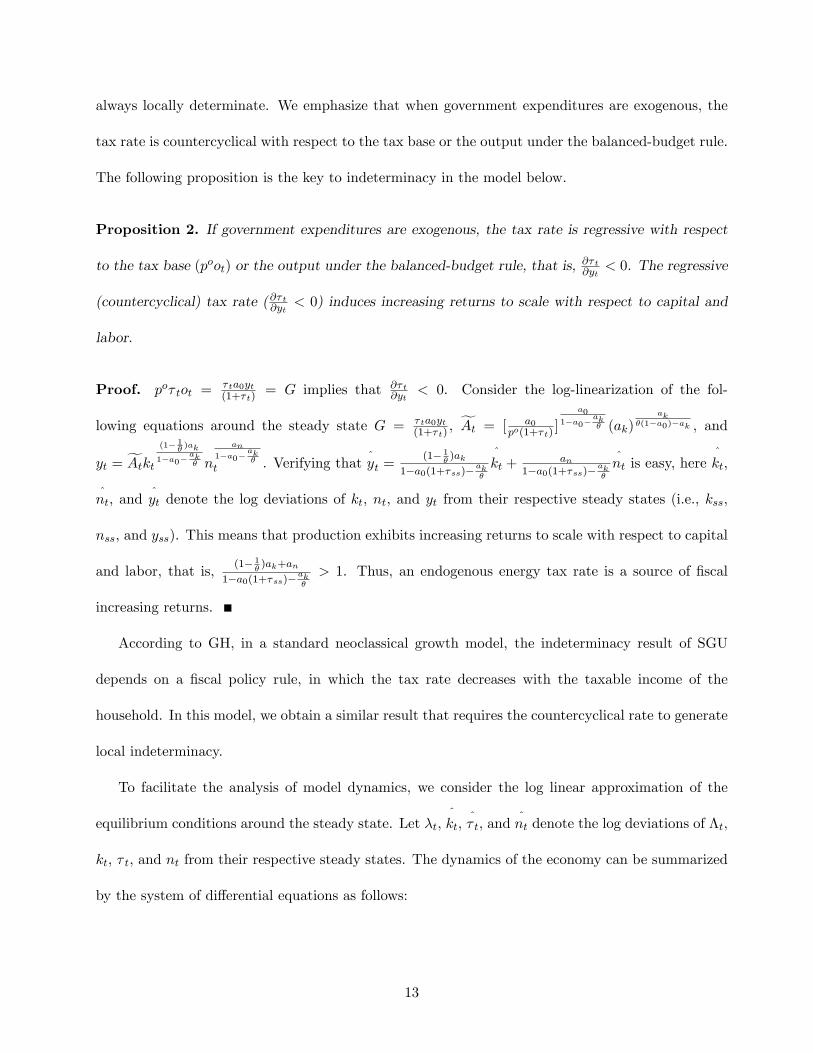
always locally determinate. We emphasize that when government expenditures are exogenous, the

tax rate is countercyclical with respect to the tax base or the output under the balanced-budget rule.

The following proposition is the key to indeterminacy in the model below.

Proposition 2. If government expenditures are exogenous, the tax rate is regressive with respect

to the tax base (poot) or the output under the balanced-budget rule, that is, @� t@yt< 0. The regressive

(countercyclical) tax rate (@� t@yt< 0) induces increasing returns to scale with respect to capital and

labor.

Proof. po� tot =� ta0yt(1+� t)

= G implies that @� t@yt

< 0. Consider the log-linearization of the fol-

lowing equations around the steady state G = � ta0yt(1+� t)

, fAt = [ a0po(1+� t)

]

a0

1�a0�ak� (ak)

ak�(1�a0)�ak , and

yt = fAtkt (1� 1�)ak

1�a0�ak� n

an

1�a0�ak�

t . Verifying that^yt =

(1� 1�)ak

1�a0(1+�ss)�ak�

^kt +

an1�a0(1+�ss)�

ak�

^nt is easy, here

^kt,

^nt, and

^yt denote the log deviations of kt, nt, and yt from their respective steady states (i.e., kss,

nss, and yss). This means that production exhibits increasing returns to scale with respect to capital

and labor, that is,(1� 1

�)ak+an

1�a0(1+�ss)�ak�

> 1. Thus, an endogenous energy tax rate is a source of �scal

increasing returns.

According to GH, in a standard neoclassical growth model, the indeterminacy result of SGU

depends on a �scal policy rule, in which the tax rate decreases with the taxable income of the

household. In this model, we obtain a similar result that requires the countercyclical rate to generate

local indeterminacy.

To facilitate the analysis of model dynamics, we consider the log linear approximation of the

equilibrium conditions around the steady state. Let �t,^kt,

^� t, and

^nt denote the log deviations of �t,

kt, � t, and nt from their respective steady states. The dynamics of the economy can be summarized

by the system of di¤erential equations as follows:

13

2664:�t:^kt

3775 =2664 �� an

ak(1� 1�)�a0�ss

�� �ssa0ak(1� 1

�)�a0�ss

�(1�a0�

ak�)

ak(1� 1�)

1�(�ss+1)a0�ak�

ak(1� 1�)�a0�ss

�(1�a0�

ak�)

ak(1� 1�)�a0�ss

37752664 �t^kt

3775 . (22)

Note that the trace and determinant of the Jacobian matrix, which determines the local dynamics

around the steady state (denoted by J), are stated as follows:

tr(J) =ak(1� 1

� )

ak(1� 1� )� a0� ss

�, (23)

det(J) =�2(1� a0 � ak

� )

[ak(1� 1� )� a0� ss]

(a0� ss � an)ak(1� 1

� ). (24)

Proposition 3. The necessary and su¢ cient condition for the model to exhibit local indeterminacy

is tr(J) < 0 < det(J), or, aka0 (1�1� ) < � ss <

ana0.

Given that the capital stock (kt) is a predetermined variable, the model is locally indeterminate

if and only if both the eigenvalues of the Jacobian matrix have negative real parts. This is equivalent

to requiring that the determinant be positive and the trace, negative. Verifying that tr(J) < 0 if and

only if � ss >aka0(1� 1

� ) is easy. If the trace condition is satis�ed, the term�2(1�a0�

ak�)

[ak(1� 1�)�a0�ss]

on the right

side of the determinant is negative. Hence, det(J) > 0 if and only if � ss < ana0. Thus, the necessary

and su¢ cient condition for the model to exhibit local indeterminacy is aka0 (1�1� ) < � ss <

ana0.

Similar to SGU, if the set of tax rates satisfying the necessary and su¢ cient condition is not empty,

a su¢ cient condition is that the labor share should be larger than the capital share (i.e., an > ak). If

the steady-state tax rates are smaller than aka0(1� 1

� ) or greater thanana0, the determinant is negative,

thereby indicating that the model exhibits local determinacy. We emphasize that SGU shows that

the revenue-maximizing tax rate is the least upper bound of the set of tax rates for which the model

is locally indeterminate; this property also holds in our case.

14

The intuition behind the indeterminacy result is straightforward. If agents expect future tax rates

to increase, then for any given capital stock, future imports must be lower. Given that @2yt@kt@ot

> 0,

the rate of return on capital becomes lower as well. The decrease in the expected rate of return on

capital may decrease the current oil demand, leading to a decrease in current output. Due to the fact

that the tax rate is countercyclical (@� t@yt< 0), budget balance increases the current tax rate, thereby

validating the initial expectations of the agents.

According to ACW (2008), heavy reliance on imported energy can induce aggregate instability in

the presence of increasing returns to scale, that is, the larger the imported energy share in the GDP,

the easier it is for the economy to be indeterminate and unstable. We have a similar proposition

expressed below.

Proposition 4. The larger the imported energy share in the GDP, the easier it is for the economy

to be indeterminate. The lower bound of the indeterminacy region aka0(1 � 1

� ) < � ss <ana0decreases

as a0 increases; thus, the larger the a0 means that indeterminacy occurs more easily in the range of

empirical tax rates.

We see that an increase in a0, either holding an constant or holding ak constant, will decrease

the term on the left-hand side, making it easier for local indeterminacy to arise.3 And the inequality

on the right-hand side does not bind for empirically plausible parameter values.

3Under the assumption that the energy is a substitute for capital, an remains constant. It means that when a0increases, ak decreases so that ak + a0 remains constant (assuming constant returns to scale at the �rm level). Underthe assumption that the energy is a substitute for labor, ak remains constant. It means that when a0 increases, andecreases so that an + a0 remains constant. Proposition 4 holds under these two assumptions. Note that if the energyis a substitute for labor, introducing energy or increasing a0, will reduce an with ak staying constant. So

aka0(1 � 1

�)

will fall. When the energy is a substitute for capital, introducing a0 will reduce ak. Hence,aka0(1� 1

�) falls by more.

15

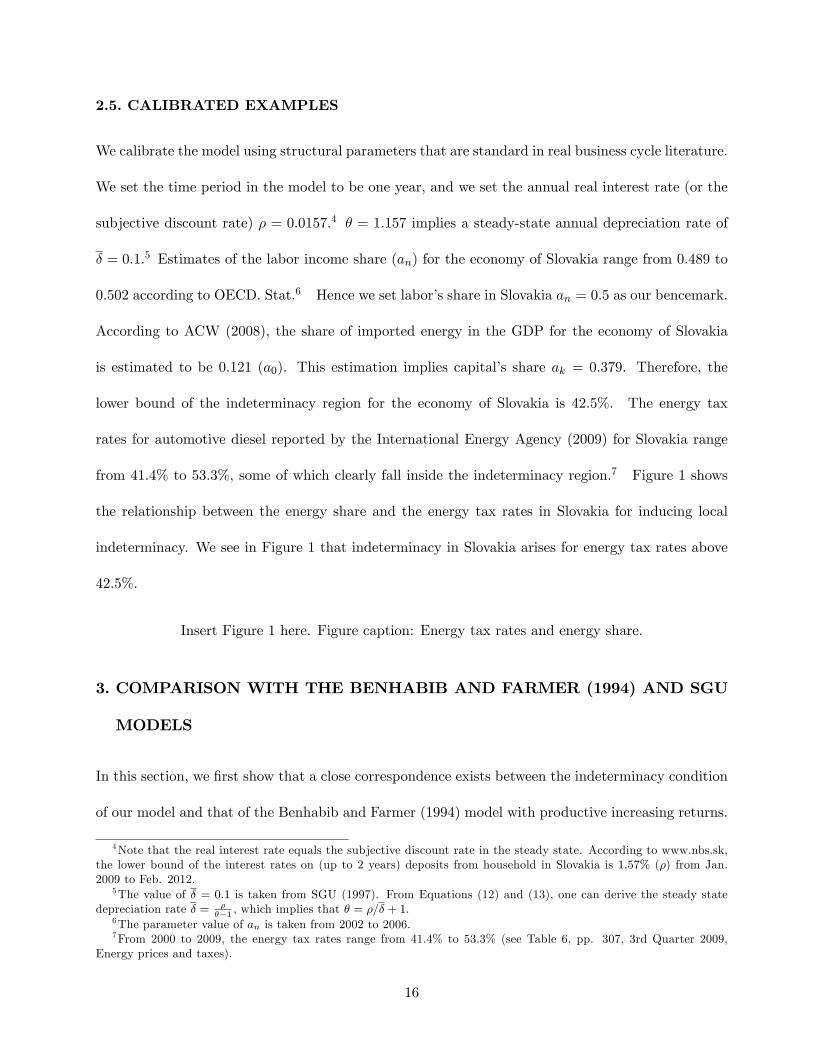
2.5. CALIBRATED EXAMPLES

We calibrate the model using structural parameters that are standard in real business cycle literature.

We set the time period in the model to be one year, and we set the annual real interest rate (or the

subjective discount rate) � = 0:0157.4 � = 1:157 implies a steady-state annual depreciation rate of

� = 0:1.5 Estimates of the labor income share (an) for the economy of Slovakia range from 0:489 to

0:502 according to OECD. Stat.6 Hence we set labor�s share in Slovakia an = 0:5 as our bencemark.

According to ACW (2008), the share of imported energy in the GDP for the economy of Slovakia

is estimated to be 0:121 (a0). This estimation implies capital�s share ak = 0:379. Therefore, the

lower bound of the indeterminacy region for the economy of Slovakia is 42:5%. The energy tax

rates for automotive diesel reported by the International Energy Agency (2009) for Slovakia range

from 41:4% to 53:3%, some of which clearly fall inside the indeterminacy region.7 Figure 1 shows

the relationship between the energy share and the energy tax rates in Slovakia for inducing local

indeterminacy. We see in Figure 1 that indeterminacy in Slovakia arises for energy tax rates above

42:5%.

Insert Figure 1 here. Figure caption: Energy tax rates and energy share.

3. COMPARISON WITH THE BENHABIB AND FARMER (1994) AND SGU

MODELS

In this section, we �rst show that a close correspondence exists between the indeterminacy condition

of our model and that of the Benhabib and Farmer (1994) model with productive increasing returns.

4Note that the real interest rate equals the subjective discount rate in the steady state. According to www.nbs.sk,the lower bound of the interest rates on (up to 2 years) deposits from household in Slovakia is 1:57% (�) from Jan.2009 to Feb. 2012.

5The value of � = 0:1 is taken from SGU (1997). From Equations (12) and (13), one can derive the steady statedepreciation rate � = �

��1 , which implies that � = �=� + 1.6The parameter value of an is taken from 2002 to 2006.7From 2000 to 2009, the energy tax rates range from 41.4% to 53.3% (see Table 6, pp. 307, 3rd Quarter 2009,

Energy prices and taxes).

16

This means that the necessary condition for local indeterminacy is that the equilibrium labor demand

schedule is upward sloping and steeper than the labor supply schedule. Unlike the model of Benhabib

and Farmer (1994), that presented in the current work relies on �scal increasing returns to yield an

upward sloping equilibrium labor demand schedule. In fact, the equilibrium labor demand schedule

in our model is upward sloping, because an increases in employment can decrease the equilibrium tax

rates and increase the after-tax return on labor. To elucidate, we write the after-tax labor demand

function as follows (in log deviations from the steady state):

^wt =

ak(1� 1� )

1� a0 � ak�

^kt �

ak(1� 1� )

1� a0 � ak�

^nt �

a01� a0 � ak

�

� ss1 + � ss

^� t, (25)

where^wt =

^btwt� a0

1�a0�ak�

�ss1+�ss

^� t is the log deviation of the after-tax wage rate from the steady state.8

The labor demand schedule of a �rm is a decreasing function of^nt. However, when we replace

^� t

with^kt and

^nt using the balanced-budget equation, obtaining the equilibrium labor demand schedule

is easy, as can be seen from the following:

^wt =

ak(1� 1� )

1� a0(1 + � ss)� ak�

^kt +

a0� ss � ak(1� 1� )

1� a0(1 + � ss)� ak�

^nt. (26)

Given that aka0 (1�1� ) < � ss <

ana0, the equilibrium labor demand function is upward sloping because

a0�ss�ak(1� 1�)

1�a0(1+�ss)�ak�

> 0. In our case,^wt =

^ct, so that the aggregate labor supply is horizontal and the

labor demand schedule is steeper than the labor supply schedule if aka0 (1�1� ) < � ss <

ana0.

Second, we compare our model with the SGU model. It must be emphasized that our economy

can easily be shown to be equivalent to the SGU model because in both cases, the price-to-cost

markup is countercyclical with respect to output, which is the key requirement in generating local

indeterminacy. However, SGU�s indeterminacy results do not depend on capacity utilization. In

8 ^btwt denotes the log deviation of the before-tax wage rate from the steady state.

17

our model, without variable capacity utilization, local indeterminacy cannot occur for empirically

plausible values of energy tax rates. For example, when � � 1, the optimal rate of capacity utilization

is always one and this model is reduced to that of Zhang (2009). The necessary and su¢ cient

conditions for the model to exhibit local indeterminacy become aka0< �Zss <

ana0. In the above

calibrated example, if the capacity utilization were �xed as in the model of Zhang, the lower bound

of the indeterminacy region would be 3:132, which makes it harder for local indeterminacy to occur.

The reason is that when the economy is subject to �scal increasing returns caused by endogenous

energy tax rates, variable capacity utilization ampli�es the aggregate returns to scale, thus making

local indeterminacy occur for mild �scal increasing returns. It is clear that the true returns to scale

with respect to capital and labor in the current model ((1� 1

�)ak+an

1�a0(1+�ss)�ak�

) are larger than those in

the corresponding model with �xed capacity utilization ( ak+an1�a0(1+�ss)). To be more precise, variable

capacity utilization increases the elasticity of output with respect to labor. And in the presence of

mild �scal increasing returns, this e¤ect can be strong enough to push the elasticity of output with

respect to labor above one ( an1�a0(1+�ss)�

ak�

> 1). Therefore, in equilibrium the marginal product of

labor is an increasing function of labor, which implies that the model is indeterminate [see, Benhabib

and Farmer (1994)].

One feature of this model is that this model requires a steeper (upward sloping) equilibrium labor

demand curve than the corresponding model [Zhang (2009)]with �xed capacity utilization to induce

local indeterminacy due to the presence of �scal increasing returns. It is clear that the slope of

the equilibrium labor demand curve in the current model (slope=a0�ss�ak(1� 1

�)

1�a0(1+�ss)�ak�

) is larger than that

in the corresponding model with �xed capacity utilization (slope= a0�ss�ak1�a0(1+�ss)). Note that variable

capacity utilization can explain why under productive increasing returns, local indeterminacy may

emerge in a one-sector growth model with a downward sloping aggregate labor demand curve [see,

Wen (1998)]. However, under �scal increasing returns, variable capacity utilization makes local

18

indeterminacy harder to occur with a downward sloping equilibrium labor demand curve.

We can understand the above result using the labor supply and demand curves. Note that

^ct =

^kt + �

^ut �

^nt holds, where

^ut denotes the log deviation of the capacity utilization rate from

its steady state. We see that the capacity utilization rate can respond to changes in consumption

level. Suppose that an increase in the initial consumption level induces an upward shift of the labor

supply curve (because^wt =

^ct). Although the capacity utilization rate increases, the equilibrium

labor demand curve (26) will not shift because this curve does not depend on^ut. Therefore, the shift

of the labor supply curve would decrease the equilibrium labor (and output) unless the equilibrium

labor demand curve was upward sloping and steeper than the labor supply curve (as in the model

of SGU). In our model, due to the presence of an upward sloping equilibrium labor demand curve,

equilibrium labor and output will increase, which substantiates the initial increase in consumption

level.

4. CONCLUSION

We explore the channel equivalence between factor income taxes and energy taxes to generate local

indeterminacy.9 The channel is determined through �scal increasing returns by endogenizing rates

and making the government spending (or lump-sum transfers) exogenous. In the presence of �s-

cal increasing returns caused by endogenous energy taxes, indeterminacy easily occurs in economies

that import foreign energy. The required steady-state energy tax rates can be empirically realistic.

An implication of this paper is that economies largely dependent on non-reproducible natural re-

sources may be vulnerable to sunspot �uctuations if the government �nances public spending with

endogenous energy taxes.

Two future research directions are as follows: (1) determining under what circumstances, energy

9As in SGU, income-elastic government spending, public debt, predetermined tax rates, and more general preferencescan be allowed. And we believe that these extensions do not change our core results.

19

taxes and capital income taxes are equivalent in generating indeterminacy, given that the essential

element for indeterminacy in the SGU model is an endogenous labor income tax rate; and (2) allowing

for international trade de�cits to o¤er important contributions to literature.

20

REFERENCES

Aguiar-Conraria, L., Wen, Y., 2007. Understanding the large negative impact of oil shocks. Journal

of Money, Credit, and Banking 39, 925�944.

Aguiar-Conraria, L., Wen, Y., 2008. A note on oil dependence and economic instability. Macroeco-

nomic Dynamics 12, 717�723.

Benhabib, J., Farmer, R.E., 1994. Indeterminacy and increasing returns. Journal of Economic

Theory 63, 19�41.

De Miguel, C., Manzano, B., 2006. Optimal oil taxation in a small open economy. Review of

Economic Dynamics 9, 438�454.

Guo, J.T., Harrison, S.G., 2004. Balanced-budget rules and macroeconomic (in)stability. Journal

of Economic Theory 119, 357�363.

Hamilton, J., 1983. Oil and the macroeconomy since World War II. Journal of Political Economy,

91:2, 228�248.

Hamilton, J., 1985. Historical causes of postwar oil shocks and recessions. Energy Journal, 6,

97�116.

Hansen, G., 1985. Indivisible labor and the business cycles. Journal of Monetary Economics 16,

309�327.

International Energy Agency, 2009. Energy prices and taxes, 3rd Quarter.

Rotemberg, J., Woodford, M., 1994. Energy taxes and aggregate economic activity. In J. Poterba

(ed.), Tax Policy and the Economy, vol. 8, Cambridge, MA: MIT Press. pp. 159�195.

21

Schmitt-Grohe, S., Uribe, M., 1997. Balanced-budget rules, distortionary taxes, and aggregate

instability. Journal of Political Economy 105, 976-1000.

Wen, Y., 1998. Capacity utilization under increasing returns to scale. Journal of Economic Theory

81, 7-36.

Zhang, Y., 2009. Tari¤and equilibrium indeterminacy. Mimeo, New York University. http://mpra.ub.uni-

muenchen.de/13099/.

22

­1 ­0.5 0 0.5 1 1.50.42

0.44

0.46

0.48

0.5

0.52

0.54

0.56

Energy share a0=0.121

Energ

y t

ax r

ate

s

2 stable roots for the economy of Slovakia

Figure 1. Energy tax rates and energy share.

23