bae systems arl-1900 antenna laas/gbas ground …arlassociates.net/baesystemsarl-1900antenna.pdfbae...

BAE Systems ARL-1900 Antenna

LAAS/GBAS Ground Reference Antenna

Alfred R. Lopez

Papers Published In

The Proceeding of the Institute of Navigation (ION)

ION NTM 26-28 January 2000 Anaheim, CA

GPS Ground Station Antenna for Local Area Augmentation System, LAAS

ION GPS 2001 11-14 September 2001 Salt Lake City, UT

Calibration of LAAS Reference Antennas

ION AM 23-25 June 2003 Albuquerque, NM

LAAS Reference Antennas – Circular Polarization Mitigates Multipath Effects

ION GNSS 21-24 September 2004 Long Beach, CA

LAAS Reference Antennas – Key Siting Considerations

ION NTM 28-30 January 2008 San Diego, CA

LAAS/GBAS Ground Reference Antenna with Enhanced Mitigation of Ground Multipath

GPS Ground Station Antennafor

Local Area Augmentation System, LAAS

Alfred R. LopezMarconi Aerospace Systems Inc.

Formerly GEC-Marconi Hazeltine Corporation

38
ION NTM 2000, 26-28 January 2000, Anaheim, CA
BIOGRAPHY

Alfred R. Lopez is a Life Fellow of the IEEE. He receiveda BEE from Manhattan College in 1958 and an MSEEfrom the Polytechnic Institute of Brooklyn in 1963. He isa Senior Mender Technical Staff at MARCONI. Hestarted his career at Wheeler Laboratories in 1958 as anantenna design specialist. He has made significantcontributions to the theory and practice of electronicscanned antennas. From 1969 to 1990 he was involvedwith the development of the Microwave Landing System.He has published several articles in IEEE publications,has been issued 29 U. S. Patents, and has received severalIEEE Awards, one being the 1988 IEEE Antennas andPropagation Society’s Harold A. Wheeler Award.

ABSTRACT

The requirements for a LAAS ground station are such thatunusual antenna specifications need to be defined andimplemented. For code tracking, the group delay variationover the coverage should be specified; this is not a typicalantenna specification. For carrier-phase tracking, thephase center variation over the coverage should bespecified; also not a typical antenna specification. Theimpulse response over the coverage should be such thatany waveform degradation is within acceptable limits.

Listed below are the key requirements for a near idealGPS Ground Station Antenna.

• Hemispherical Coverage (down to 3° elevation)• Right Hand Circular Polarization Over Entire

Coverage• 3 dB/Degree Cutoff at Horizon• Sidelobes > 23 dB Down from Peak in Lower

Hemisphere• Point Phase Center• Point Group-Delay Center

A concept that incorporates some of these features wasdeveloped in 1996, U. S. Patent, 5,534,882 [1]. Morerecent developments have resulted in an antenna

7

configuration that incorporates all of the desired features.This paper presents the basic concept disclosed in theissued patent and the additional attributes of the improveddesign. Such an antenna has been developed. It operatesat the L1 and L2 frequencies. Measurements ofbreadboard and production prototype antennas haveverified the performance.

INTRODUCTION

Multipath represents the dominant error source insatellite-based precision guidance systems [2]. For LAASthe mulitpath delay at the reference antenna is less than 15meters. The design of the ground station referenceantenna is key in the mitigation of multipath errorsassociated with these short delays. A good deal of efforthas been expended in developing antenna solutions to thisproblem [3,4,5]. One solution [3,4] utilizes two antennasto provide the required hemispherical coverage.

Figure 1. Ground Station Antenna -- Model ARL-2100

21 Elements, 11 Elements Excited11-Way Power Divider at Base

Equal-Line-Length Cables to Elements

This approach requires two receivers for each referenceantenna and a somewhat complex process for handoffbetween antennas. The antenna described in this paper(see Figure 1) requires one receiver and offers otheradvantages with respect to processing satellites at lowelevation angles.

ACCURACY AND ANTENNA PARAMETERS

The LAAS ground facility, LGF, consists of a smallcollection of high quality GPS reference receivers andantennas at known, surveyed locations on the airportproperty. The receiver measurements at the surveyedlocations are used to determine an average correction thatis broadcast to approaching aircraft using a VHF datalink. A set of tentative requirements for precisionapproach using LAAS is presented in [6]. This set ofrequirements indicates that a 2-sigma (95 percentprobability) error of 1 meter is required for control of theaircraft under fault free conditions and for systemintegrity and continuity. The table shown in Figure 2presents an allocation of this 1-meter error toleranceamongst the LAAS components. Most of the allowableerror is allocated to the airborne subsystem component.

Figure 2. System Accuracy Allocation

Allowable Error95 PercentProbability(Meters)

1. System / Integrity / Continuity(Root Sum Square Allocationamongst 2 & 3)

1.00

2. Airborne Subsystem 0.94

3. LAAS Ground Facility CorrectionReceiver ProcessingAntenna

MultipathPhaseGroup Delay

Root Sum Square

0.22

0.250.050.050.34

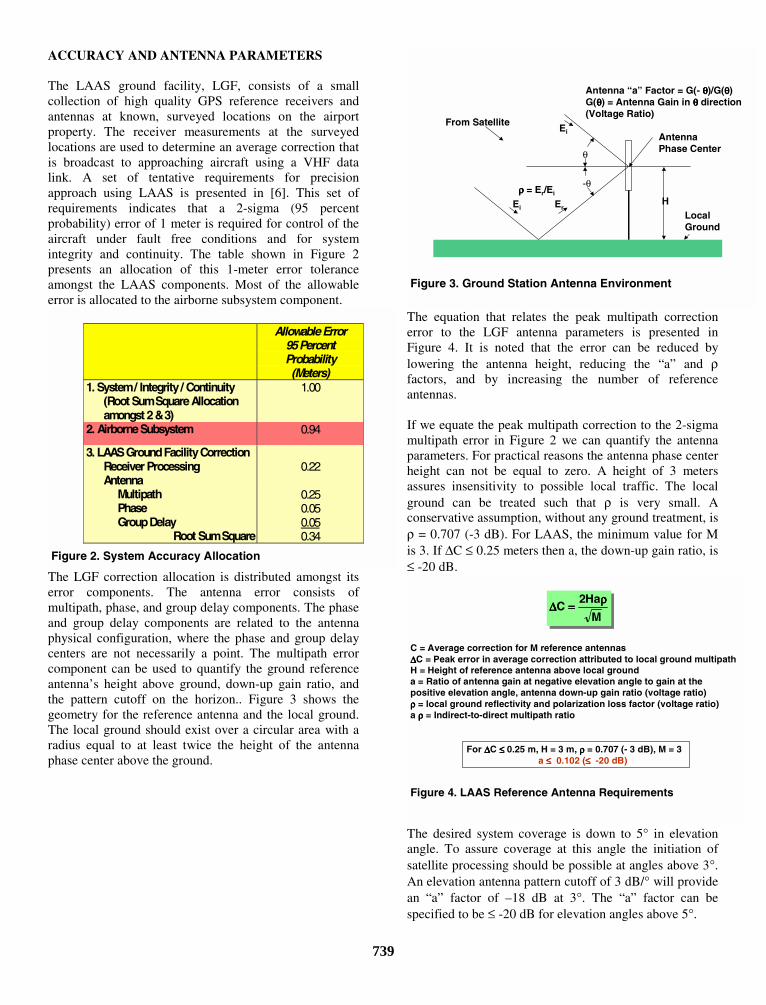
The LGF correction allocation is distributed amongst itserror components. The antenna error consists ofmultipath, phase, and group delay components. The phaseand group delay components are related to the antennaphysical configuration, where the phase and group delaycenters are not necessarily a point. The multipath errorcomponent can be used to quantify the ground referenceantenna’s height above ground, down-up gain ratio, andthe pattern cutoff on the horizon.. Figure 3 shows thegeometry for the reference antenna and the local ground.The local ground should exist over a circular area with aradius equal to at least twice the height of the antennaphase center above the ground.

739

Figure 3. Ground Station Antenna Environment

θ

From Satellite

H

-θ

AntennaPhase Center

Ei Er

ρρρρ = Er/Ei

Antenna “a” Factor = G(- θθθθ)/G(θθθθ)G(θθθθ) = Antenna Gain in θθθθ direction(Voltage Ratio)

Ei

LocalGround

The equation that relates the peak multipath correctionerror to the LGF antenna parameters is presented inFigure 4. It is noted that the error can be reduced bylowering the antenna height, reducing the “a” and ρfactors, and by increasing the number of referenceantennas.

If we equate the peak multipath correction to the 2-sigmamultipath error in Figure 2 we can quantify the antennaparameters. For practical reasons the antenna phase centerheight can not be equal to zero. A height of 3 metersassures insensitivity to possible local traffic. The localground can be treated such that ρ is very small. Aconservative assumption, without any ground treatment, isρ = 0.707 (-3 dB). For LAAS, the minimum value for Mis 3. If ∆C ≤ 0.25 meters then a, the down-up gain ratio, is≤ -20 dB.

Figure 4. LAAS Reference Antenna Requirements

C = Average correction for M reference antennas∆∆∆∆C = Peak error in average correction attributed to local ground multipathH = Height of reference antenna above local grounda = Ratio of antenna gain at negative elevation angle to gain at thepositive elevation angle, antenna down-up gain ratio (voltage ratio)ρρρρ = local ground reflectivity and polarization loss factor (voltage ratio)a ρρρρ = Indirect-to-direct multipath ratio

M

Ha2C

ρρρρ====∆∆∆∆

For ∆∆∆∆C ≤≤≤≤ 0.25 m, H = 3 m, ρρρρ = 0.707 (- 3 dB), M = 3 a ≤≤≤≤ 0.102 (≤≤≤≤ -20 dB)

The desired system coverage is down to 5° in elevationangle. To assure coverage at this angle the initiation ofsatellite processing should be possible at angles above 3°.An elevation antenna pattern cutoff of 3 dB/° will providean “a” factor of –18 dB at 3°. The “a” factor can bespecified to be ≤ -20 dB for elevation angles above 5°.

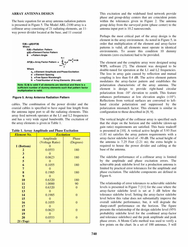
ARRAY ANTENNA DESIGN

The basic equation for an array antenna radiation patternis presented in Figure 5. The Model ARL-2100 array is acollinear array consisting of 21 radiating elements, an 11-way power divider located at the base, and 11 coaxial

Figure 5. Array Antenna Radiation Pattern

odd) is (N Elements Arrayof Number Total Nh WavelengtSpace Free

Spacing Element dExcitation Phase and plitudeElement Am a

Where

ea Pattern Factor Array )AF(

AnglePattern Pattern FactorElement )g(

Pattern Radiation )E(Where

)(AF)(g)(E

n

21N

21N

n

)sin(d

n2jn

========λλλλ========

========θθθθ

====θθθθ====θθθθ====θθθθ

θθθθθθθθ====θθθθ

∑∑∑∑

−−−−

−−−−−−−−====

θθθθλλλλ

ππππ

Note: E( θ θ θ θ) is valid if all elements are identical and there is asufficient number of dummy elements such that pattern factormultiplication is valid.

cables. The combination of the power divider and thecoaxial cables is specified to have equal line length fromthe antenna input port to all the radiating elements. Thisarray feed network operates at the L1 and L2 frequenciesand has a very wide signal bandwidth. The excitation ofthe array elements is given in Table 1.

Table 1. Array Amplitude and Phase ExcitationElement No. Excitation

Amplitude(Voltage Ratio)

Phase(Degrees)

1 (Bottom) 02 0.0553 1803 04 0.0623 1805 06 0.1055 1807 08 0.1985 1809 0

10 0.6320 18011 1.0000 9012 0.6320 013 014 0.1985 015 016 0.1055 017 018 0.0623 019 020 0.0553 0

21 (Top) 0

740

This excitation and the wideband feed network providephase and group-delay centers that are coincident pointswithin the tolerances given in Figure 2. The antennagroup delay from the surveyed point (phase center) to theantenna input port is 10.2 nanoseconds.

Perhaps the most critical part of the array design is theelement in the array environment. As noted in Figure 5, inorder that multiplication of the element and array-factorpatterns is valid, all elements must operate in identicalenvironments. To assure this condition 10 dummyelements (zero excitation) had to be provided.

The element and the complete array were designed usingWIPL software [7]. The element was designed to bedouble-tuned for operation at the L1 and L2 frequencies.The loss in array gain caused by reflection and mutualcoupling is less than 0.4 dB. The active element patternmodulates the array-factor pattern and establishes thepolarization characteristic of the array antenna. Theelement is design to provide right-hand circularpolarization from -10° elevation to zenith. This featureenhances performance at low elevation angles (<10°).Reflections from vertical surfaces are converted to left-hand circular polarization and suppressed by thepolarization mismatch factor. This element is similar inconfiguration to those described in [8, 9].

The vertical height of the collinear array is specified suchthat the slope on the horizon and the sidelobe (down-upgain ratio) requirements are satisfied. This basic tradeoffis presented in [10]. A vertical active height of 5.93 Feet(1.81 m) satisfies the array pattern requirements with aarray-factor sidelobe level of –30 dB. The actual height ofthe antenna is 7.25 Feet (2.21 m); the extra height isrequired to house the power divider and cabling at thebase of the antenna.

The sidelobe performance of a collinear array is limitedby the amplitude and phase excitation errors. Theachievable peak sidelobe level for a production antenna islimited by practical error tolerances for the amplitude andphase excitation. The sidelobe components are defined inFigure 6.

The relationship of error tolerances to achievable sidelobelevels is presented in Figure 7 [11] for the case where thearray-factor sidelobe level is set at 3 dB below thetolerance sidelobe level. Setting the array-factor sidelobelevel below this value does not substantially improve theoverall sidelobe performance, but, it will degrade thesharp-cutoff performance on the horizon. The figurepresents the relationship of the design sidelobe level (95%probability sidelobe level for the combined array-factorand tolerance sidelobes) and the peak amplitude and peakphase errors. A Monte Carlo method was used to verify afew points on the chart. In a set of 100 antennas, 5 will

have one sidelobe above the design sidelobe value. Forconvenience, the amplitude error, expressed as a voltageratio, is set equal to the phase error in radians.

ToleranceSidelobe Level

SLT RMS sidelobe component attributed toarray excitation amplitude and phaseerrors

Array-FactorSidelobe Level

SLAF Peak sidelobe component for error-freearray excitation

DesignSidelobe Level

SLD Desired peak sidelobe level (95 percentprobability that combined components(SLT and SLAF) will not exceed SLD)

Figure 6. Array Performance Limited by Tolerances

)3

21(G

32

SL2

2

Tδ−

δ

=δδδδ = Peak amplitude error (voltage ratio)δδδδ = Peak phase error (radians)G = Directive Gain (G = 2 forhemispherical coverage)

Figure 7 indicates that the required tolerances for –40 dBsidelobes (±0.1dB amplitude and ±0.5° phase) areimpossible to achieve, the required tolerances for –30 dBsidelobes (±0.2dB amplitude and ±0.1.6° phase) are reallynot practical, while the tolerances for –23 dB sidelobes(±0.6dB amplitude and ±0.3.6° phase) are achievable.

40 38 36 34 32 30 28 26 24 22 200

0.5

1

1.5

2

2.5

3

3.5

4

4.5

5

PeakAmplitudeand Phase

Error

Tolerance

Phase (Degrees)

Amplitude (dB)

Design Sidelobe Level (dB)(95 % Probability Peak Sidelobe Level)

Figure 7. Array Performance Limited by Tolerances, Cont’d

Figure 8 shows the computed array factor patterns forzero errors and one case for an peak amplitude error of0.5 dB, uniformly distributed between –0.5 dB and 0.5dB, and an peak phase error of 5°, uniformly distributedbetween -5° and 5°.

Figure 9 shows the result of the WIPL computer softwaresimulation [7] of the complete 21-element array. Thesimulation includes mutual coupling effects. It does notinclude amplitude and phase errors. Note that the elementfactor modulates the array-factor envelope and that a dipin the pattern exists at 70° elevation.

741

Figure 8. Array Factor Pattern

90 80 70 60 50 40 30 20 10 0 10 20 30 40 50 60 70 80 9040

35

30

25

20

15

10

5

0

5

90 80 70 60 50 40 30 20 10 0 10 20 30 40 50 60 70 80 9040

35

30

25

20

15

10

5

0

5

Elevation Angle (Degrees)

dB

Amp. Error = ±±±± 0.5 dBPhase Error = ±±±± 5 Deg.

Amp. Error = 0 dBPhase Error = 0 Deg.

90 80 70 60 50 40 30 20 10 0 10 20 30 40 50 60 70 80 9040

35

30

25

20

15

10

5

0

5

Figure 9. Computer Simulation of 21-Element Array Antenna

TotalRadiation

(dBi)


Right HandCircular

PolarizationHorizontal

LinearPolarization

Left HandCircular

Polarization

Figure 10 shows computed and measured installed patternfor the Model ARL-2100 brassboard. The computedpattern is generated using the equation:

)sin(H2

2je)(E)(E)(F

θλ

π−θ−−θ=θ

Amplitude and phase excitation errors are included in thearray pattern. H = 1.3 meters. The measured pattern [12]is obtained by recording and plotting the carrier-to-noise-density ratio versus elevation angle for several satellitesover a 24-hour period. The brassboard antenna wasinstalled at a site with the antenna phase center at a 1.3-meter height. The green curve in Figure 9 is the plot forone representative satellite, PRN 6. One part of the curveis the data for the time interval between satellite rise andzenith times; the other is for the time interval betweenzenith and set times. The displacement between the twocurves is indicative of the lack of complete omni-directionality of the brassboard antenna. The multipathelevation lobing factor has a maximum of ±0.75 dB. Thiscorresponds to a multipath indirect-to-direct ratio of –21dB. For comparison the installed patterns for a choke-ringantenna (blue curves) were measured. The improved

performance of the Model ARL-2100, at low elevationangles, is clearly evident.

Figure 10. Installed Performance

0 1 0 2 0 3 0 4 0 5 0 6 0 7 0 8 0 9 02 5

3 0

3 5

4 0

4 5

5 0

5 5

M ic ro p u ls e c h o k e rin g

H a z e lt in e P h a z a r

0 10 20 30 40 50 60 70 80 9025

30

35

40

45

50

55

Carrier-to-Noise-Density Ratio Versus Elevation Angle

ComputedAmplitude & Phase Errors

Included

dBHz


MeasuredModel ARL-2100 Brassboard

Raytheon, PRN 6 11/99

±±±± 0.75 dB Peak Lobing Factor(-21 dB Indirect/Direct Ratio)

SUMMARY

• A concept for a near ideal ground station antenna forLAAS augmentation systems has been described.

• A practical and affordable antenna has beendeveloped

• A brassboard and 5 production prototype antennashave been built and tested

• Field testing has verified the design• L1 and L2 operation has been demonstrated

ACKNOWLEDEMENTS

The author is much appreciative of the motivation andsupport of Jack Flynn, Marconi. The concept for thepractical array implementation is credited, in part, toEdward Newman and Richard Kumpfbeck of Marconi.Marshall Wax, of Marconi, was the lead engineer for thedesign, implementation and testing of the Model ARL-2100 antenna. The motivation and help provided by PaulKline and Rod Stangeland of Honeywell, and the helpprovided by Tom Zaugg, of Raytheon, is appreciated.

REFERENCES[1] A. R. Lopez, “GPS Antenna System,” U. S. Patent

5,534,882, Jul. 9, 1996.[2] M. S. Braasch, “Multipath Effects,” Chap. 14 in

“Global Positioning System: Theory andApplication,” Eds. Parkinson and Spilker, AIAA,Vol. 1, 1996.

[3] M. Braasch, “Optimum antenna design for DGPSground reference stations,” Proc. ION GPS-97, pp.1291-1297.

[4] C. Bartone, F. van Graas, “Airport psuedolite forprecision approach applications,” Proc. ION GPS-97,pp. 1841-1850.

[5] C. C. Counselman, III, “Multipath-Rejecting GPSAntennas,” Proceedings of the IEEE, Vol. 87, No. 1,pp. 86-91, Jan. 1999.

742

[6] P. Enge, “Local Area Augmentation of GPS for thePrecision Approach of Aircraft,” Proceedings of theIEEE, Vol 87, No. 1, pp. 111-132, Jan. 1999.

[7] B. M. Kolundzjia, J. S. Ognjanovic, T. K. Sarkar, R.F. Harrington, “WIPL: A program forElectromagnetic Modeling of Composite Wire andPlate Structures,” IEEE Ant. & Prop. Magazine, Vol.38, No. 1, Feb. 1996.

[8] N. E, Lindenblad, “Antenna and Transmission Linesat the Empire State Television Station,”Communications, 21, 10-14, 24-26, April 1941

[9] O. M. Woodward, “Circularly-Polarized AntennaSystem Using Tilted Dipoles,” U. S. Patent4,083,051, Apr. 4, 1978

[10] A. R. Lopez, “Sharp Cutoff Radiation Patterns,”IEEE Trans. Ant. & Prop, Vol. AP-27, No. 6, pp.820-824, Nov. 1979.

[11] R. C. Hansen, “Phased Array Antennas,” Wiley, pp.465-470, 1998.

[12] T. Zaugg, Raytheon email, Nov. 19, 1999

Calibration of LAAS Reference Antennas

Alfred R. Lopez

BAE SYSTEMS Advanced Systems

BIOGRAPHY Alfred R. Lopez is a Life Fellow of the IEEE. He received a BEE from Manhattan College in 1958 and an MSEE from the Polytechnic Institute of Brooklyn in 1963. He is a Hazeltine Fellow at BAE SYSTEMS Advanced Systems. He started his career at Wheeler Laboratories in 1958 as an antenna design specialist. He has made contributions to the theory and practice of electronic scanned antennas. From 1969 to 1990 he was involved with the development of the Microwave Landing System. He has published extensively in IEEE publications, has been issued 33 US Patents, and has received several IEEE Awards; one being the 1988 IEEE Antennas and Propagation Society’s Harold A. Wheeler Award. ABSTRACT The Differential GPS, DGPS, Local Area Augmentation System, LAAS, utilizes reference antennas and receivers to measure the time of arrival of GPS signals at precisely surveyed points. These measurements are then used to broadcast differential corrections to approaching aircraft. A common misconception is to assume that the antenna phase center is the precise point whose position is being measured. The antenna phase center (or equivalent carrier phase-delay center) is a well defined concept: “The location of a point associated with an antenna such that, if it is taken as the center of a sphere whose radius extents into the far-field, the phase of a given field component over the surface of the radiation sphere is essentially constant, at least over that portion of the surface where the radiation is significant,” (IEEE definition). The antenna phase center is defined at one frequency, the carrier frequency. For GPS reference antennas, a new antenna concept, the antenna group phase center (or equivalent code phase center) should be defined. Thus, the antenna has two phase centers, the carrier phase center and the code phase center. These phase centers are not necessarily points and the two phase-delay centers may or

may not have the same characteristics. Typically, they do not have the same characteristics. This paper introduces the concepts of code-phase delay and carrier-phase delay as related to the calibration of LAAS reference antennas. It describes the characteristics of one candidate type of reference antenna for LAAS. It discusses the results of some recent field measurements of antenna code-phase-delay minus carrier-phase-delay. It also discusses the measurements of code and carrier phase delays, which may be used to calibrate GPS reference antennas. INTRODUCTION The Local Area Augmentation System is a local differential GPS, DGPS, system that is being developed by the Federal Aviation Administration and the aviation industry to support high-precision aircraft approach procedures. It consists of a small collection of high-quality GPS receivers and antennas at known, surveyed locations on an airport property. LAAS determines range corrections that are broadcast to approaching aircraft. The airborne receiver uses these measurements to correct it’s own measurements to achieve sub-meter accuracy. The reference antennas have stringent accuracy requirements; the error directly attributed to the antennas should not exceed a few centimeters. The antennas, like other system components, have a transmission-line type delay that is included with the delays of the other components in the basic calibration of the system. The special errors associated with the antennas that are of concern in this paper are the errors that are angle dependent. These errors are related to the inherent variation with angle of the antenna “carrier phase center” and the antenna “code (group) phase center.” The antenna phase center is a well defined concept [1], “The location of a point associated with an antenna such that, if it is

taken as the center of a sphere whose radius extents into the far-field, the phase of a given field component over the surface of the radiation sphere is essentially constant, at least over that portion of the surface where the radiation is significant,” (IEEE definition). The writer is not aware of a definition for the antenna “group (code) phase center” and is proposing that the IEEE definition of phase center be used to define code phase center by replacing the words, “the phase of a given field component,” by “the code phase of a given field component.” Before defining code phase center, the code phase must be defined. The antenna carrier-phase and code-phase centers are not necessarily the same point. For DGPS the observables of interest are the code phase delay and the carrier phase delay. The code delay is equal to the signal modulation or group delay, and is equal to the rate of change of phase with respect to angular frequency (dϕ/dω). The antenna code delay should be used to measure the code pseudorange correction. The carrier delay is defined at the carrier frequency, and is equal to the total phase divided by the angular frequency (-ϕ/ω). For LAAS calibration purposes, measurement of the code delay variation, over the antenna coverage region, is a requirement. An outline of the paper is presented below: • Overview of Calibration Process • The Antenna Phase Centers • Rudimentary Antenna Example • BAE SYSTEMS Model ARL-1500 Antenna • Antenna Calibration Methodology • Summary

SatelliteSurveyed

Point

Ground AntennaSurveyed

Point

ReceiverTime-of-ArrivalMeasurement

TIME

PseudorangeDelay

CalibrationDelay

Calibration Components:Antenna Angle-Dependent DelayAntenna Constant DelayFilter and LNA DelayTransmission Line DelayReceiver Delay


SatelliteSurveyed

Point

Ground AntennaSurveyed

Point

ReceiverTime-of-ArrivalMeasurement

TIME

PseudorangeDelay

CalibrationDelay



Figure 1. Pseudorange Measurement OVERVIEW OF CALIBRATION PROCESS Some basic elements for a pseudorange measurement are shown in Figure 1. It is assumed that the time-of-departure of the code epoch from the surveyed point at the satellite is known. The time-of-arrival of the code epoch at the ground antenna surveyed point can not be measured directly because of intervening components that add delay to the measurement. These components, constant and

angle-dependent, are indicated in Figure 1. The magnitude of the code (group) delay for the constant components can be determined and subtracted from the time-of-arrival as measured at a point within the receiver. The antenna angle-dependent code-delay component is characteristic of the antenna in a manner analogous to the typical antenna angle-dependent amplitude and phase characteristics. An antenna range measurement is required to determine the code delay (phase) variation with angle. This measurement can be used to reduce the pseudorange correction error associated with the antenna angle-dependent code-delay component.

Group (Code) Delay

Antenna Patterns

Amplitude

CW (Carrier) Delay

Group (Code)Phase Center

CW (Carrier)Phase Center

Phase (ϕ = -2πft)

c = Speed of light f = Carrier frequency

IEEE Definition No IEEE Definition ( ) GPS Terminology

dfd

2πcDcode

ϕ=

f2πc-Dcarrierϕ

=

Group (Code) Delay

Antenna Patterns

Amplitude

CW (Carrier) Delay

Group (Code)Phase Center

CW (Carrier)Phase Center

Phase (ϕ = -2πft)

c = Speed of light f = Carrier frequency

IEEE Definition No IEEE Definition ( ) GPS Terminology

dfd

2πcDcode

ϕ=

f2πc-Dcarrierϕ

=

Figure 2. Antenna Angle Dependence THE ANTENNA PHASE CENTERS The angle-dependent variations of an antenna are described in terms of antenna patterns, the spatial distribution of a quantity that characterizes the electromagnetic field generated by an antenna [1]. As shown in Figure 2, antenna patterns can be either amplitude or phase patterns. Phase patterns are divided into two subclasses, CW delay and group delay. The IEEE defines the concept of antenna phase center with respect to CW radiation [1] where phase center is synonymous with carrier phase center. For DGPS there is a need to define another fundamental antenna characteristic, the antenna code (group) phase center. To define the code phase center it is first necessary to define code phase. Proposed definitions for code phase and code phase center are presented in Figure 3. Some basic characteristics associated with the carrier phase center and the code phase center are presented in Figure 4. In the evolution of DGPS, the common perception was that of the antenna phase center. This concept should now be expanded to the notion of the antenna phase centers, the carrier phase center and the code phase center.

The location of a point associated with an antenna such that, if it is taken as the center of a sphere whose radius extends into the far-field, the code phase of a given field component over the surface of the radiation sphere is essentially constant, at least over that portion of the surface where the radiation is significant. Note: Some antennas do not have a unique code phase center.(This proposed code phase center definition is identical to the IEEE definition for phase center with the word “phase” replaced by “code phase.”)

Code Phase Center

For GPS, the ratio of the code delay, in units of time, to the code repetition period.

Code Phase

The location of a point associated with an antenna such that, if it is taken as the center of a sphere whose radius extends into the far-field, the code phase of a given field component over the surface of the radiation sphere is essentially constant, at least over that portion of the surface where the radiation is significant. Note: Some antennas do not have a unique code phase center.(This proposed code phase center definition is identical to the IEEE definition for phase center with the word “phase” replaced by “code phase.”)

Code Phase Center

For GPS, the ratio of the code delay, in units of time, to the code repetition period.

Code Phase

Figure 3. Proposed Definition – GPS Code Phase Center

Phase centers may or may not be a point.


Phase centers may or may not be the same.


If one phase center is a point, then, the carrier and code phase centers are the same point.

Typically, there is significant variations and significant difference in the variations of the

carrier and code phase centers

The highest possible DGPS accuracy is achieved by calibration of the reference antenna phase centers.






If one phase center is a point, then, the carrier and code phase centers are the same point.

Typically, there is significant variations and significant difference in the variations of the

carrier and code phase centers



Figure 4. Phase Center Characteristics Some recent measurements at the FAA William J. Hughes Technical Center have shown a systematic relationship between the variation of the mean-value of code-minus-carrier pseudorange error and the antenna amplitude pattern [3]. It is believed by the writer that this relationship can be explained by a comparison of the amplitude variation to the inherent variation in the difference between the code and carrier phase centers. This will be discussed in more detail in the following sections.

Turnstile:2 Crossed λ/2 Dipoles Fed in Time Quadrature

Disk

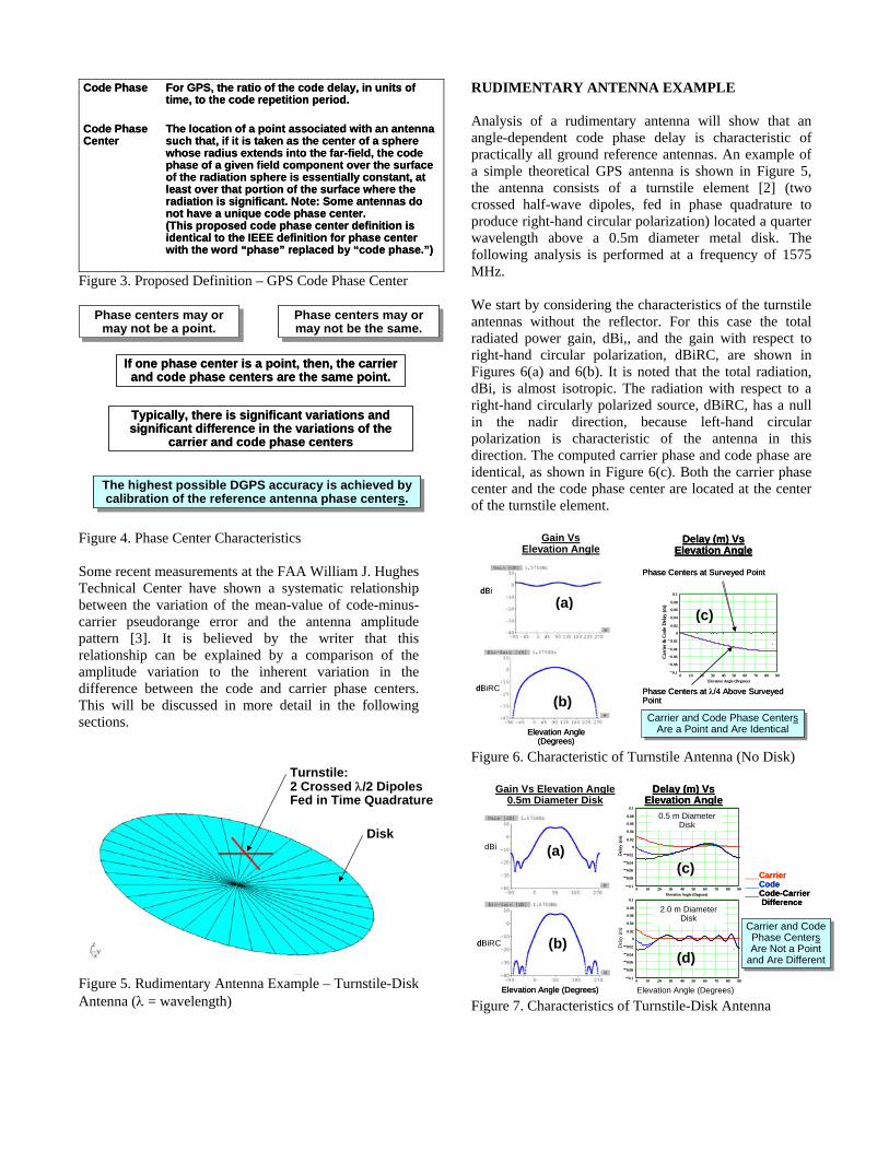
Figure 5. Rudimentary Antenna Example – Turnstile-Disk Antenna (λ = wavelength)

RUDIMENTARY ANTENNA EXAMPLE Analysis of a rudimentary antenna will show that an angle-dependent code phase delay is characteristic of practically all ground reference antennas. An example of a simple theoretical GPS antenna is shown in Figure 5, the antenna consists of a turnstile element [2] (two crossed half-wave dipoles, fed in phase quadrature to produce right-hand circular polarization) located a quarter wavelength above a 0.5m diameter metal disk. The following analysis is performed at a frequency of 1575 MHz. We start by considering the characteristics of the turnstile antennas without the reflector. For this case the total radiated power gain, dBi,, and the gain with respect to right-hand circular polarization, dBiRC, are shown in Figures 6(a) and 6(b). It is noted that the total radiation, dBi, is almost isotropic. The radiation with respect to a right-hand circularly polarized source, dBiRC, has a null in the nadir direction, because left-hand circular polarization is characteristic of the antenna in this direction. The computed carrier phase and code phase are identical, as shown in Figure 6(c). Both the carrier phase center and the code phase center are located at the center of the turnstile element.

0.06

0.08

0.1

(m)

dBi

dBiRC

Eleva(D

Gain Vs Elevation Angle

Delay (m) Vs Elevation Angle

Phase Centers at Surveyed Point

0.06

0.08

0.1

(m)

dBi

dBiRC

Eleva(D

Gain Vs Elevation Angle


Phase Centers at Surveyed Point

Figure 6. Cha

dBi

dBiRC

Elevation An

Gain Vs El0.5m Dia

dBi

dBiRC

Elevation An

Gain Vs El0.5m Dia

Figure 7. Cha

(a)

0 10 20 30 40 50 60 70 80 900.1

0.08

0.06

0.04

0.02

0

0.02

0.04


Car

rier &

Cod

e D

elay

.

tion Angle egrees)

Phase Centers at λ/4 Above Surveyed Point

Carrier and Code Phase CentersAre a Point and Are Identical


0 10 20 30 40 50 60 70 80 900.1

0.08

0.06

0.04

0.02

0

0.02

0.04


Car

rier &

Cod

e D

elay

.

tion Angle egrees)

Phase Centers at λ/4 Above Surveyed Point



)

)

racteristic of Turnstile Antenna (No Disk)

evation Angle meter Disk


0.02

0

0.02

0.04

0.06

0.08

0.1

Del

ay (m

)

.

0.5 m Diameter Disk

evation Angle meter Disk


0.02

0

0.02

0.04

0.06

0.08

0.1

Del

ay (m

)

.

0.5 m Diameter Disk
(a)
(b

___Carrier___Code___Code-Carrier

Difference

0.04

0.02

0

0.02

0.04

0.06

0.08

0.1

Del

ay (m

)

.

0 10 20 30 40 50 60 70 80 900.1

0.08

0.06

0.04


Carrier and Code Phase CentersAre Not a Point


2.0 m Diameter Disk

___Carrier___Code___Code-Carrier

Difference

0.04

0.02

0

0.02

0.04

0.06

0.08

0.1

Del

ay (m

)

.

0 10 20 30 40 50 60 70 80 900.1

0.08

0.06

0.04




2.0 m Diameter Disk

)

)
(b
gle (Degrees)0 10 20 30 40

0.1

0.08

0.06

Elevation AnElevation Anggle (Degrees)0 10 20 30 40

0.1

0.08

0.06

Elevation AnElevation Ang

racteristics of Turnstile-

(c

(c

and Are Differentand Are Differentand Are Differentand Are Different)
(d 50 60 70 80 90
gle (Degrees)le (Degrees)50 60 70 80 90

gle (Degrees)le (Degrees) Disk Antenna

Radiation patterns for the turnstile-disk antenna are shown in Figures 7(a) and 7(b). The disk creates the pattern cutoff near the horizon (0° and 180° elevation angles). The phase characteristics are also shown in Figure 7(c). The antenna reference point is at the center of the disk. Of special interest is the difference between the code and carrier phase delays. Above 30° of elevation angle, the carrier phase delay is nearly constant, which is characteristic of the antenna if the disk diameter is large. The disk creates an image of the turnstile antenna and the resulting 2-element array has a carrier phase center at the center of the disk. It is noted that the code phase delay has significant variation over the complete range of elevation angle. This variation is attributed to diffraction by the rim of the disk. The diffraction component acts like multipath with a delay that is approximately equal to:

))cos(1(RDDif θ−= Where R = Disk radius θ = Elevation angle

This multipath-like component creates a variation of the code delay with elevation angle. This is more clearly illustrated in Figure 7(d), which shows the variation for the case of a disk with a 2m diameter. One can observe the increased number of cycles in the code phase variation associated with diffraction from the rim of a larger diameter disk. Appendix A provides an independent theoretical verification of the code-carrier difference variation of rudimentary antennas. The key result is the observation that the addition of a reflector to the turnstile antenna, which has identical code and carrier phase characteristics, creates a significant difference in the code and carrier phase characteristics. It is expected that most GPS LAAS reference antennas have code and phase characteristics that differ significantly. The code-phase variation should be used for the calibration of DGPS reference antennas. The carrier-phase variation should be used for the calibration of antenna systems that only utilize the carrier phase in their operation. The key electrical specifications for a centimeter-accuracy DGPS reference antenna are presented below. • Gain (dBiRC) over coverage volume (upper

hemisphere) • Up-down gain ratio (dB) (ratio of total radiated

power, provides suppression of ground multipath) • Antenna reference points (x-y-z-coordinates of the

average carrier phase center and the average code phase center)

• Carrier phase center variation (mm) over coverage volume (calibration data for measurements that utilize carrier phase)

• Code phase center variation (cm) over coverage volume (calibration data for measurements that utilize the code epoch)

BAE SYSTEMS MODEL ARL-1500 ANTENNA An antenna was conceived in 1995 [4], which was intended for application as a GPS ground reference antenna. The key features of this antenna are: • Single port coverage of upper hemisphere with right

hand circular polarization • Sharp pattern cutoff at horizon for acquisition of

satellites at low elevation angles • High up/down gain ratio for suppression of ground

multipath error • Operation at L1 and L2 frequencies Several prototypes of this antenna have been fabricated [5] and tested at various facilities. An initial evaluation indicates that this antenna shows promise of satisfying the requirements for DGPS ground reference antenna systems. Key to its performance is the reduction of angle-dependent code delay error by means of calibration. Computer

Model Prototype

Figure 8. BAE SYSTEMS Model ARL-1500 Antenna An FAA William J. Hughes Technical Center report [3] describes a trend in the mean of the code-minus-carrier measurement of the pseudorange error that is related to the antenna gain (amplitude) pattern for the Multipath Limiting Antenna [9]. The report indicates that the trend would impact error characterization. It speculates that the trend is related to amplitude and that perhaps some parameter, such as AGC, could remove the trend. The writer believes that the trend is not directly related to amplitude but, rather, it is related to a fundamental difference between the code-delay and carrier-delay antenna patterns and, that the trend can be removed by calibration of the antenna.

The computer model (see Figure 8) that was used for the initial design of the Model ARL-1500 antenna was used to compute the code-carrier difference delay pattern. Antenna phase patterns were computed at two frequencies separated by 10 MHz. The code-carrier difference delay pattern is then computed using the formulas given in Figure 2. This pattern was then compared to the computed amplitude pattern. Shown in Figure 9 are the computed gain patterns; the total gain, dBi, and the gain with respect to a right-hand circularly polarized source, dBiRC. It is noted that over the upper hemisphere (0° to 180° elevation angles) the dBi and dBiRC responses are nearly identical. This indicates that the antenna has essentially right hand circular polarization over the upper hemisphere. The dBiRC gain pattern was converted to carrier-to-noise-density ratio pattern and is presented in Figure 10. Figure 10 also shows the code, carrier and code-carrier difference delay patterns with elevation angle. One can see a definite relationship between the amplitude (gain) variation and the code-carrier difference variation. It is this type of relationship that was observed in the FAA William J. Hughes Technical Center measurements [3]. If the antenna code-delay variation with elevation angle can be determined then it is possible to eliminate this pseudorange correction error component by a calibration process. It is noted that the code delay (phase) pattern is a fundamental antenna characteristic, as is the antenna amplitude pattern and the carrier delay (phase) pattern. They exhibit similar traits. It is also noted that the use of “B Values” [8] to assess the performance of ground reference antennas could result in significant error and degradation of system integrity. The “B Values” is a comparison of pseudorange corrections from several reference antennas, and is a measure of the integrity of the LAAS Ground Facility, LGF, in a multipath environment. A within-specification difference in the pseudorange corrections amongst the reference antennas is intended to indicate high integrity. If the accuracy of a particular antenna type is determined by a “B Value” assessment of a group of antennas, then, if all antennas have identical and out-of-tolerance variation of code delay with antenna angle and the multipath environment is benign, the antennas would be judged to have acceptable performance. This is because at any antenna angle they would all have the same pseudorange correction error associated with the code delay variation with antenna angle. For this case the LGF would lack integrity because it is broadcasting within specification conditions when in fact the pseudorange corrections have out-of-tolerance errors. What is needed is an independent assessment of each antenna to ensure that the angle-

(a)

)

Figure 9. BAtotal gain, dBrespect to rig

0 10 2035

40

45

50

55

E

Car

rier-

to-N

oise

Rat

io (d

B-H

z)

Carrier-to-N(

5 dB

Elevatio0 10 20

35

40

45

50

55

E

Car

rier-

to-N

oise

Rat

io (d

B-H

z)

Carrier-to-N(

5 dB

Elevatio

Figure 10. BComputer SCode Delay

(b

(c)

E SYSTEMS Model ARL-1500 Antenna (a) i, polar plot (b) total gain, dBi (c) gain with

ht-hand circular polarization, dBiRC

30 40 50 60 70 80 90levation Angle (Degrees)

.

oise-Density Ratio dB-Hz)

Delay (meters):___Carrier___Code

___Code-Carrier Difference

0 10 20 30 40 50 60 70 80 900.2

0.15

0.1

0.05

0

0.05

0.1

0.15

0.2


Del

ay (m

)

.

0.05 Meters/Unit/Unit

n Angle (Degrees) Elevation Angle (Degrees)30 40 50 60 70 80 90levation Angle (Degrees)

.

oise-Density Ratio dB-Hz)

Delay (meters):___Carrier___Code

___Code-Carrier Difference

0 10 20 30 40 50 60 70 80 900.2

0.15

0.1

0.05

0

0.05

0.1

0.15

0.2


Del

ay (m

)

.

0.05 Meters/Unit/Unit

n Angle (Degrees) Elevation Angle (Degrees) AE SYSTEMS Model ARL-1500 Antenna – imulations – Amplitude, Carrier Delay, and Patterns

dependent error is within specification. A calibration process may be needed to satisfy the requirements. ANTENNA CALIBRATION METHODOLOGY Measuring the code delay variation over angle, and using this data for calibration of the antenna, will reduce the antenna angle-dependent error associated with the code delay variation. To minimize the magnitude of the code delay variation over the coverage volume the physical reference point (surveyed point) should be at or near the median value of the code phase center evaluated over the desired coverage volume. The measurement of code delay variation can be performed at an antenna range or on a site using the satellite constellation. In either case, the measurement is somewhat difficult to perform. A high-quality antenna range is required for measuring the antenna code delay pattern. An outline of the two alternatives for code-delay measurements is presented below. • Conventional Antenna Test Range − Very high quality (ideally –50 dB reflection level) − Measurements – Gain pattern, up-down ratio pattern,

carrier delay pattern, and code delay pattern • Site Installation Using GPS Constellation As Source

Radiation − Far-field pattern (20,000Km) − Satellite provide near constant illumination at ground

level − Measurements – Carrier-to-noise-density ratio

pattern, code-delay minus carrier-delay pattern, carrier delay pattern

− Azimuth angle variation Three 24 hour periods with antenna rotated 120° each 24 hour period One 24 hour period with several 360° continuous antenna rotations in 24 hour period

Antenna Range Measurement The specification for one type of antenna range, suitable for the measurement of code delay, is given in Table 1.

Elevation-Plane Pattern Pivot Point

θ

Incident Plane Wave

H

Nominal Phase Center

Back-Wall Reflection Surfaceρ = 0.01 (-40 dB)

R

Antenna Under Test

Elevation AngleBack-Wall Reflection

Surface (-40dB)

Antenna Under Test

Incident Plane Wave Nominal

Phase CenterElevation–Plane

Pattern Pivot Point

Elevation Angle


θ

Incident Plane Wave

H



R

Antenna Under Test

Elevation Angle


θ

Incident Plane Wave

H



R

Antenna Under Test

Elevation AngleBack-Wall Reflection

Surface (-40dB)

Antenna Under Test

Incident Plane Wave Nominal

Phase CenterElevation–Plane

Pattern Pivot Point

Elevation Angle

Figure 11. Test zone geometry for tapered anechoic chamber Table 1. Antenna Test Range Specifications Type range Tapered anechoic chamber Axial length 30m Test zone dimensions

6m height 6m width 6m length

Back wall reflection factor

< -40 dB

Frequency range 1565 to 1585 MHz 1217 to 1237 MHz

Frequency steps 2.0 MHz Antenna positions Elevation, 0° to 90° in 0.2° steps

Azimuth, 0° to 360° in 2° steps Code phase delay error (rms)

< 0.01m

To evaluate the range error the antenna is assumed to have a point carrier-phase center and a point code-phase center that are coincident as shown in Figure 11. The back wall reflection is the dominant error component for a tapered anechoic chamber. The antenna-range carrier phase error is given by [11]:

⎥⎥⎥⎥⎥

⎦

⎤

⎢⎢⎢⎢⎢

⎣

⎡

⎥⎦⎤

⎢⎣⎡ +θπ

ρ+ρ+

⎥⎦⎤

⎢⎣⎡ +θπ

ρ−=θϕ −

)R)sin(H(c

f4cos21

)R)sin(H(c

f4sinsin),f(

ar2

ar

ar1

Where ρar = Antenna-range reflection factor = ρud ρ = 0.0018 (-55 dB) ρud = Antenna up/down ratio factor = 0.18 (-15 dB) ρ = Back wall reflection factor = 0.01 (-40 dB) The equations presented in Figure 2 are used to compute the carrier delay and the code delay. The range error variation with elevation angle is shown in Figure 12. It is noted that the standard deviation for the range code-delay error is less than 0.01meters, which is considered to be suitable for the measurement of the code delay pattern. Site Measurement Using Satellite Constellation The satellite constellation and antenna site can be visualized as the largest antenna test range ever conceived. It has a far-field distance of approximately 20,000Km and the signal level at the test site is nearly constant for all satellites independent of their position in space., Amplitude, carrier delay, and code delay, antenna patterns are measured by rotating the reference antenna about its vertical axis and recording data during a test period (one to several days). The antenna rotation can be

continuous or stepped. Each data point has an azimuth angle and elevation angle tag. The data points are sorted

Carrier-to-Noise-Density Ratio (dB-Hz)

Computed

0 10 20 30 40 50 60 70 80 9035

40

45

50

55


Car

rier-

to-N

oise

-Den

sity

Rat

io (d

B-H

z)

.

FAA Tech Center Data


dB-Hz35

40

45

50

55

0 10 20 30 40 50 60 70 80 90Elevation Angle (Degree s)

Carri

er-to

-Noi

se D

ensi

ty R

atio

(dB-

Hz)

0 20 40 60 80

0.04

0.02

0

0.02

0.04


Phas

e D

elay

(m)

.

Code Carrier

Figure 13. Amplitude versus elevation angle The BAE SYSTEMS Model ARL-1500 antenna was measured at the FAA William J. Hughes Technical Center. The antenna (with conical ground plane) was installed at the LAAS Test Prototype (LTP) field site at one of the four established LTP antenna locations. GPS observables were collected using the Novatel Millennium GPS Receiver and a laptop computer. An Astech Z-XII connected to an Ashtech survey ground plane antenna was used to collect L1-L2 data for estimation of the ionospheric divergence. Data was collected in 24-hour periods to allow for observation of the full constellation at the site. The data samples have 100 seconds of carrier smoothing and a sample period of 200 seconds.

Figure 12. Antenna range delay error versus elevation angle, H = 1.5m, R = 3m, f = 1575 MHz, and ρar = 0.0018 into azimuth and elevation bins and processed to generate the desired antenna patterns. Rotation about the vertical axis provides the means for reducing site multipath effects by averaging over many multipath scenarios. Code-minus-carrier measurements [6], using the satellite constellation, have been used to quantify the pseudorange correction errors; assuming that the carrier-delay errors are negligible. This type of measurement can be used to determine the error variations that are characteristic of the reference antenna.

Smoothed CMC Mean vs. 2 Degree Elevation Bins for 10 Degree Azimuth BinsBAE Antenna - w/ Conical Ground Plane (non-extended)

Data Collection: 11/11/00, ACY LT2, 24 Hours of Data

-0.8

-0.6

-0.4

-0.2

0

0.2

0.4

0.6

0.8

0 10 20 30

CMCMean(meters)

102030405060708090100110120130140150160170180190200210220230

Smoothed CMC f

BAE Antenna - wData Collection

0

0.05

0.1

0.15

0.2

0.25

0.3

0 10 20 3

SMOOTHEDCMCSTD.DEV.(METERS)

Smoothed Code Minus Carrier2° El B

BAE An

Data Co

Z

S

ins for 10° Az Binst.– w/Conical Ground Plane

(non-ellection: 11/11/00, ACY LT2,

xtended)

Mean vs. El & A

td. D

Smoothed CMC Mean vs. 2 Degree Elevation Bins for 10 Degree Azimuth BinsBAE Antenna - w/ Conical Ground Plane (non-extended)

Data Collection: 11/11/00, ACY LT2, 24 Hours of Data

-0.8

-0.6

-0.4

-0.2

0

0.2

0.4

0.6

0.8

0 10 20 30

CMCMean(meters)

102030405060708090100110120130140150160170180190200210220230

Smoothed CMC f

BAE Antenna - wData Collection

0

0.05

0.1

0.15

0.2

0.25

0.3

0 10 20 3

SMOOTHEDCMCSTD.DEV.(METERS)

Smooth2° El B

BAE An

Data Co

Z

S

ed Code Minus Carrierins for 10° Az Bins

t.– w/Conical Ground Plane(non-e

llection: 11/11/00, ACY LT2,xtended)

Mean vs. El & AMean vs. El & Az

td. D

Smoothed Code Minus Carrier 2° El Bins for 10° Az Bins

BAE Ant. – w/Conical Ground Plane (non-extended)

Data Collection: 11/11/00, ACY LT2,

Std.

Figure 14. Model ARL-1

40 50 60 70 80 90Elevation Bin (Degrees)

240250260270280290300310320330340350360

Std. Dev. vs. 2 Degree Elevation Binsor 10 Degree Azimuth Bins/ Conical Ground Plane (non-extended): 11/11/00, ACY LT2, 24 Hours of Data

102030405060708090100110120130140

24 Ho

Z

urs of Data

. vs. El & A 0.2

0.25

0.3

CodeMinusCarrier(M

Std Dev

C-Curve

Smoothed CMC Std. Dev. vs. 2 Degree Elevation BinsBAE Antenna - w/ Conical Ground Plane (non-extended)

Data Collection: 11/11/00, ACY LT2, 24 Hours

C-Curve

40 50 60 70 80 90Elevation Bin (Degrees)

240250260270280290300310320330340350360

Std. Dev. vs. 2 Degree Elevation Binsor 10 Degree Azimuth Bins/ Conical Ground Plane (non-extended): 11/11/00, ACY LT2, 24 Hours of Data

102030405060708090100110120130140

24 Ho

Z

urs of Data

. vs. El & A 0.2

0.25

0.3

CodeMinusCarrier(M

Std Dev

C-Curve



C-Curve0.2

0.25

0.3

CodeMinusCarrier(M

Std Dev

C-Curve



C-Curve0.2

0.25

0.3

CodeMinusCarrier(M

Std Dev

C-Curve



C-Curve0.2

0.25

0.3

CodeMinusCarrier(M

Std Dev

C-Curve



C-Curve

24 Hours of Data (a)

C-Curve . vs. El & Az
evevDev
0 40 50 60 70 80 90

ELEVATION ANGLE (DEGREES)

150160170180190200210220230240250260270280290300310320330340350360

0

0.05

0.1

0.15

0 10

eters)

Std ev.

Elev0 40 50 60 70 80 90

ELEVATION ANGLE (DEGREES)

150160170180190200210220230240250260270280290300310320330340350360

0

0.05

0.1

0.15

0 10

eters)

Std ev.

0

0.05

0.1

0.15

0 10

eters)

Std ev.

0

0.05

0.1

0.15

0 10

eters)

Std ev.

0

0.05

0.1

0.15

0 10

eters)

Std ev.

Ele

St ev. (b)

vE

500 antenna accuracy with elevation and azimuth

. D. D. D. D. Dd. D

20 30 40 50 60

ELEVATION ANGLE(DEGREES)

ation Angle (D20 30 40 50 60

ELEVATION ANGLE(DEGREES)20 30 40 50 60



ELEVATION ANGLE(DEGREES)

(c)

ation Angle (Dlevation Angle (D

calibration

of Dataof Dataof Dataof Dataof Data

70 80 90

)egrees70 80 9070 80 9070 80 9070 80 90

)egreesegrees)

Figure 13 shows a comparison of the Tech Center and computed amplitude versus elevation angle. The code-minus-carrier, CMC, mean versus 2°-elevation bins for 10°-azimuth bins is shown in Figure 14(a). This data set was further smoothed and interpolated to provide a complete set of calibration data for the complete range of azimuth and elevation angles. An analysis of the data (see Figure 15) indicates that that there is substantial systematic variation of the mean with azimuth. Because of the small size of the antenna in the horizontal plane, it is believed that the variation attributed to the antenna has a one-cycle variation in 360°. The indications are that an elevation-only calibration would not be satisfactory. A 2-dimensional (azimuth angle and elevation angle) calibration appears to be required for the BAE SYSTEMS Model ARL-1500 antenna.

0 60 120 180 240 300 3600.4

0.2

0

0.2

0.4

.

0 60 120 180 240 300 3600.4

0.2

0

0.2

0.4

Mean(m)

Azimuth Angle (Degrees)

0.54m


Estimated Calibration

Residual Calibration

Error(m)

0 60 120 180 240 300 3600.4

0.2

0

0.2

0.4

.

0 60 120 180 240 300 3600.4

0.2

0

0.2

0.4

Mean(m)


0.54m


Estimated Calibration

Residual Calibration

Error(m)

Figure 15. Mean pseudorange error versus azimuth angle at an elevation angle of 68° for BAE SYSTEMS Model ARL-1500 antenna Figure 14(b) presents CMC standard deviation data for the same set of data presented in Figure 14(a). If it is assumed that the azimuth variation of the mean is characteristic of the antenna, then it can be removed by calibration. For this situation the standard deviation versus elevation angle can be computed for each 2°-elevation bin by computing the rms of the standard deviations for the 36 10°-azimuth bins. Figure 14(c) presents the results of this computation. Shown in Figure 14(c) is the so-called “C-Curve” LAAS accuracy requirement for one reference antenna [8]. A Model ARL-1500 antenna system accuracy budget is presented in Table 2. The budget includes a 0.08-meter allocation for a residual error associated with the calibration process. The budget indicates that the Model ARL-1500 antenna system could satisfy the LAAS Ground Facility accuracy requirement with some margin if the angle-dependent code-delay error calibration is successfully implemented.

Table 2. Model ARL-1500 Antenna System Accuracy Budget Sigma Pseudorange

Correction Accuracy (Meters)

Noise & Multipath 0.10 Antenna with Calibration 0.08

Root Sum Square 0.13 Requirement:

El Angle < 35° El Angle = 90°

(See C-Curve in Figure 14(c))

≤ 0.24 ≤ 0.16

SUMMARY • The central theme of this paper is that the common

perception of the antenna phase center should be expanded. It should be recognized and appreciated that there exists two phase-centers that have significance and relevance for DGPS. The usual phase (carrier phase) center is well defined. This paper proposes a definition for the code (group) phase center.

• Over the antenna coverage region, the average carrier phase center should be designated as the carrier phase center and the average code phase center should be designated as the code phase center.

• The antenna code-delay pattern can be measured at a very high-quality antenna range, or at a site using the satellite constellation. The site may be a convenient one or the actual operational LAAS site.

• Measurements of the antenna angle-dependent code delay can be used as calibration data that, in principle, reduces the antenna angle-dependent DGPS pseudorange correction error to zero.

• An elevation and azimuth calibrated BAE SYSTEMS Model ARL-1500 single-port L1-L2 antenna shows promise of satisfying the LAAS, WAAS, JPALS and CORS requirements.

ACKNOWLEGEMENTS Special credit is given to Dave Lamb of the FAA William J. Hughes Technical Center; he was the first to observe a relationship between the code-minus-carrier delay characteristics and the reference antenna amplitude characteristics. The help provided by Dave Lamb, John Warburton and Mark Dickinson (all with the same FAA group) with the collection, processing, and interpretation of field data is greatly appreciated. At BAE SYSTEMS Advanced Systems, Edward Newman, Conrad Koch and Gary Nolan provided support, encouragement and help.

APPENDIX A: CODE-CARRIER DIFFERENCE VARIATION DEMONSTRATED BY SIMPLE DIFFRACTION ANALYSIS OF RUDIMENTARY 2-DIMENSIONAL ANTENNA The radiation pattern for a 2-dimensional antenna consisting of a magnetic line source located at the center and directly above a perfectly conducting infinite strip, is relatively simple to compute using elementary diffraction theory [12] [13] [14]. Figure A2 present a Mathcad program that computes the code-carrier difference variation.

Magnetic Line Source θ

)

Fi

Car

rier P

hase

(Rad

ians

)

arg E 1575 θ,( )(

90 0 90 180 2700

0.5

1

1.5


Am

plitu

de (V

olta

ge R

atio

)

E 1575 θ,( )

θ

E f θ,( ) 14

1 sgn θ( )+( ) 1 sgn 180 θ−( )+( )⋅⎡⎣ ⎤⎦ Dif f θ,( ) exp j− 2⋅ π⋅ d⋅ ⋅⎡⎢⎣

⋅−

Dif1 f θ,( )− exp j− 2⋅ π⋅ d⋅fc⋅ 1 cos θ

π

180⋅⎛⎜

⎝⎞⎠

+⎛⎜⎝

⎞⎠

⋅⎡⎢⎣

⎤⎥⎦

⋅+

:=

Dif1 f θ,( ) tanhv f 180 θ−,( ) v f 180 θ−,( )4

exp 1.5− v f 180 θ−,( )⋅( )⋅−⎛⎜⎝

⎞⎠

:=

Dif f θ,( ) tanhv f θ,( ) v f θ,( )4

exp 1.5− v f θ,( )⋅( )⋅−⎛⎜⎝

⎞⎠

sgn θ( )⋅ exp j−π

4⋅ ⋅⎛⎜

⎝⋅:=

tanhv f θ,( ) if θ 012,

tanh (2 v⋅

,⎛⎜⎝

:=v f θ,( ) 2 π⋅ dfc⋅⋅ sin

θπ

180⋅

2

⎛⎜⎜⎝

⎞

⎠⋅:=

θ 90− 89−, 270..:=d 1:=c 299.792458:=

Figure A2. Mathcad program for computing code-carrier differe__carrier delay __code delay __code-carrier difference, strip wi

0 10 20 30 40 500.1

0.08

0.06

0.04

0.02

0

0.02

0.04

0.06

0.08

0.1

Dcode 1575 θ,( ) Dcarr 1575 θ,( )−

Dcode 1575 θ,( )

Dcarr 1575 θ,( )

θ

DcCode Delay:Dcarr f θ,( ) c−2 π⋅ f⋅

arg E f θ,( )( )⋅:=Carrier Delay:

Perfectly Conducting Infinite Strip (Width = 2d

gure A1. 2-D antenna geometry

90 0 90 180 2704

2

0

2

4

Elevation Angle (Degress)

)

θ

fc

1 cos θπ

180⋅⎛⎜

⎝⎞⎠

−⎛⎜⎝

⎞⎠

⋅ ⎤⎥⎦...

sgn 180 θ−( )⋅ exp j−π

4⋅ tanh

v f 180 θ−,( )2.4

⎛⎜⎝

⎞⎠

⋅⎛⎜⎝

⎞⎠

⋅

tanhv f θ,( )

2.4⎛⎜⎝

⎞⎠⎞⎠

sgn θ( ) if θ 0≥ 1, 1−,( ):=v f θ,( ))f θ,( )

⎞⎠

nce variation for rudimentary 2-D antenna; dth = 2 meters, frequency = 1575 MHz

60 70 80 90

ode f θ,( ) c2 π⋅ f

arg E f θ,( )( )dd⋅:=

d = strip half width (m)f = frequency (MHz)c = speed of light (m/ µs)

REFERENCES [1] IEEE Std 100-1996, “The IEEE Standard Dictionary

of Electrical and Electronics Terms,” 6th Edition, 1996

[2] J. D. Kraus, “Antennas,” McGraw-Hill, pp. 424-428, 1950

[3] D. Lamb, “Long Term LTP Error Variation Characterization,” FAA William J. Hughes Technical Center Report, Feb. 24, 2000

[4] A. R. Lopez, “GPS Antenna System,” U. S. Patent 5,534,882, Jul. 9, 1996

[5] A. R. Lopez, “GPS Ground Station Antenna for Local Area Augmentation System, LAAS,” ION Proc. Of the 2000 National Technical Meeting, Anaheim, CA, Jan. 26-28, 2000

[6] M. S. Braasch, “Multipath Effect,” Chapter 14, “Global Positioning System: Theory and Application,” Vol. 1, B. W. Parkinson, J. J. Spilker, Editors, AIAA, pp. 560-566, 1996

[7] A. R. Lopez, “Scanning-Beam Microwave Landing System – Multipath-Errors and Antenna-Design Philosophy,” IEEE Transaction on Antennas and Propagation, vol. AP-25, No. 3, 1977

[8] Federal Aviation Administration, “Specification - Category I Local Area Augmentation System – Non-Federal Ground Facility,” FAA/AND710-2937, May 31, 2001

[9] C. Bartone, F. van Graas, “Airport Pseudolite for Precision Approach Applications.” Proc. Of ION GPS-97, Kansas City, MO, pp. 1841-1850, Sept. 16-19, 1997

[10] H. A. Wheeler, A. R. Lopez, “Multipath Effects in Doppler MLS,” Multipath Section of Hazeltine Report 10926, “Five Year Microwave Landing System Development Program Plan,” September 1972; Hazeltine Reprint H-222; October 1974

[11] C. C. Counselman, “Multipath-Rejecting GPS Antennas,” Proceeding of the IEEE, Vol. 87, No. 1, pp. 86-91. Jan. 1999.

[12] A. R. Lopez, “The Geometrical Theory of Diffraction Applied to Antenna Pattern and Impedance Calculations,” IEEE Transactions on Antennas and Propagation, vol. AP-14, No. 1, pp. 40-45, Jan. 1966.

[13] A. R. Lopez, “Application of Wedge Diffraction Theory to Estimating Power Density at Airport Humped Runways,” IEEE Transactions on Antennas and Propagation, vol. AP-35, No. 6, pp. 708-714, Jun. 1987.

[14] A. R. Lopez, “Cellular Telecommunications: Estimating Shadowing Effects Using Wedge Diffraction,” IEEE Antennas & Propagation Magazine, Vol. 40, No. 1, pp. 53-57, Feb. 1998

LAAS Reference Antennas – Circular Polarization Mitigates Multipath Effects

Alfred R. Lopez

ARL Associates

BIOGRAPHY Alfred R. Lopez is a Life Fellow of the IEEE. He received a BEE from Manhattan College in 1958 and an MSEE from the Polytechnic Institute of Brooklyn in 1963. He is a Hazeltine Fellow at BAE SYSTEMS Advanced Systems. ARL Associates is his private consulting practice. He started his career at Wheeler Laboratories in 1958 as an antenna design specialist. He has made contributions to the theory and practice of electronic scanned antennas. From 1969 to 1990 he was involved with the development of the Microwave Landing System. He has published extensively in IEEE publications, has been issued 36 US Patents, and has received several IEEE and BAE SYSTEMS Awards. ABSTRACT Early in the development of the local Area Augmentation System, LAAS, vertical linear polarization was selected for the low-elevation-angle antenna of the two-antenna reference antenna system. The initial LAAS development concentrated on ground reflected multipath. Polarization was not an issue; the level of radiation in the lower hemisphere was specified such that the ground-reflected multipath error was within acceptable limits. However, as LAAS approaches the deployment phase, other siting issues are coming to the forefront, and, polarization selection can make a significant difference. This paper reviews the issue of polarization with regard to multipath performance, and in particular, it considers the performance with respect to lateral multipath (reflections from airport objects not including ground reflection). It presents some theoretical models and past experience that demonstrate that, lateral multipath for the case of linear polarization, can cause large errors, and in some cases, can capture the receiver with an associated outlier-type error. It is concluded that if both linearly and circularly polarized antennas can satisfy the ground reflection

performance requirements then circular polarization is advantageous since it provides substantial suppression of lateral multipath effects. INTRODUCTION Signals from satellites at low elevation angles will reflect off lateral multipath (typically vertical surfaces such as aircraft fuselages and tail fins, hangars, terminal buildings, control towers, maintenance vehicles, etc.). In addition, some multipath reflector geometries or possible shadowing by objects near the horizon, can amplify the multipath (indirect) signal. This can result in the LAAS reference receiver locking on and tracking the multipath signal, with an associated large error. This condition may be steady state or transient in nature. Circular polarization mitigates the situation, since reflections nominally have the opposite handedness of circular polarization. Basically, reflections off of lateral multipath are specular in nature, and a right circularly polarized signal is reflected as a left circularly polarized signal. If the omni-directional reference antenna has right circular polarization for all directions in the upper hemisphere, then significant suppression of lateral multipath errors can be expected. (Circular polarization with an axial ratio of 1dB can provide 25 dB suppression of the reflected signal.) There are several situations in which lateral multipath can capture (multipath signal greater than the direct signal) the reference receiver. Some of these are: • Reflector Size – In electromagnetics and optics it is

well known that a Fresnel zone circular plate can cause a reflection that is 6dB stronger than the direct signal. A reflecting surface with a size that exceeds ½ Fresnel Zone has the potential to cause a reflection the amplitude of which exceeds that of the direct signal.

• Ground Profile Difference Between Direct and Indirect Signals – At low elevation angles, the ground

profile, such as rising terrain in the direction of the satellite, can suppress the direct signal with respect to the indirect signal. This is in essence, partial shadowing of the direct signal.

• Shadowing of Direct Signal – An object, such as a light pole, directly in the line-of-sight of the direct signal, can cause sufficient shadowing such that the amplitude of a reflection from an object that is normally less than that of the direct signal, now, because of shadowing of the direct signal, exceeds that of the direct signal.

This paper describes the severity of the lateral multipath problem and suggests that polarization discrimination be incorporated in the design of the reference antenna to mitigate the problem. A circularly polarized LAAS reference antenna provides significantly better multipath performance, especially for satellites at low elevation angles. A circularly polarized antenna with good ground-reflection performance has been described [1], [2], [3]. AIRPORT LATERAL MULTIPATH In this paper, lateral multipath is defined as all multipath sources excluding the ground reflection (see Figure 1). In the early 70’s a good deal of work was done in analyzing and estimating the effects of lateral multipath for the then developing Microwave Landing System, MLS, [4], [5]. Much of that work is directly applicable and helpful in estimating multipath effects for the LAAS reference antenna system. In those days computer simulations were not readily available and analysis was used to estimate performance. The airport environment has not changed very much over the years and the findings of the studies in the 70’s are still applicable.

030124 arl-3

Airport Multipath

• Local Ground• Lateral Multipath

• Aircraft Tailfin• Aircraft Fuselage• Airport Control Tower• Hangars• Terminal Buildings• Buses• Maintenance Vans• Surrounding Skyline

Figure 1 Characteristic of lateral multipath phenomena is reflection and shadowing. In combination, a multipath reflection from one object and direct-signal blocking by another object can cause the reference receiver to track the delay

of the reflecting object. In general, this is a gross error that would be detected by the integrity monitor. It could, however, affect the system availability. It is also possible that a reflecting object is large enough and close enough so that the reflected (multipath, M) signal is stronger than the direct, D, signal (M/D > 0dB). Another possible situation for an M/D > 0dB is when the direct signal is partially shadowed by a rising terrain in the direction of the satellite or by a small object, such as a light pole, directly on the line-of-sight. The M/D > 0dB situation is a significant problem that requires consideration in the LAAS operation. A more typical situation is the case of M/D < 0dB. A reflector with an M/D of –30dB and a delay ranging between 30m and 270m can cause a psuedorange error of about 0.5m (see Figure 2, and [6], page 560). For LAAS this is a significant error (the LAAS total system accuracy is less than 2m, 2-sigma). The following section describes the characteristics of objects that can cause M/D ratios ranging from –30dB to +6dB. The objective is to indicate the severity of the lateral multipath problem and that mitigation is needed.

030124 arl-4

Weak Multipath Can Cause Significant LAAS Error

δ = ρ k D / 2

δ = Peak code delay errorρ = M/D (Multipath/Direct Signal Voltage Ratio)D = Chip period = 293mk = Receiver processing factor

For k = 0.1 (Narrow correlator receiver and delays of 30-270m)

δ = ρ 14.7m

For ρ = 0.032 (-30dB) δ = 0.47m

Figure 2 ESTIMATES OF M/D RATIO In [4] a relatively simple model was developed for estimating the reflection factor, ρ (M/D voltage ratio), for a multipath object. At the point of reflection a reference reflector is located. The reference reflector is a very large flat specular surface that creates a perfect image of the antenna. As shown in Figure 3, a product of five factors gives the reflection factor for a multipath reflector: The factor, g, is the relative antenna gain in the directions of the satellite and the reflector. The factor, d, is a distance ratio factor, the ratio of the distance from the antenna to the satellite and the distance from the antenna image to the satellite. For GPS, d = 1. Three factors; size, curvature and reflectivity complete the model. This paper will concentrate on the size and curvature factors.

030625 arl-6

Simple Model for Estimating M/D

Reference Antenna

Reference Antenna Image

Multipath Reflector

Satellite

Reference Reflector – Large Flat Specular Surface Tangent to Multipath Reflector at Point of Reflection

ρ = M/D = g d ρSize ρCurvature ρReflectivity (Voltage Ratio)g = Antenna Gain Factord = Distance Factor (= 1 for GPS)ρSize = Size FactorρCurvature = Curvature FactorρReflectivity = Reflectivity Factor (non-metal and

rough surfaces)

Figure 3 The Fresnel Zone Disc is an excellent example to illustrate the severity of the lateral multipath problem; it can create an M/D ratio of +6dB. Figure 4 defines the Fresnel Zone Disc. In general, a reflector with a projected area that exceeds the ½ Fresnel Zone area has the potential to create an M/D ≥ 0dB.

030124 arl-7

Fresnel Zone Disk ρSize = 2 (+6dB)

A flat elliptical plate whose projected area is a circle with

R = Antenna-to-plate distanceλ = Free space wavelength

Antenna

Multipath Interference Pattern(Vertical λ/2 Dipole Antenna)

At the center of the reflection zone the multipath signal is 6dB stronger than the direct signal. The receiver locks onto the reflector; the error is equal to R.


Gain(dBi)

RλRadius =

NOT TO SCALE

Figure 4 Figures 4 presents the results of a computer simulation demonstrating that, as predicted by theory, a Fresnel Zone Disc can produce a +6dB M/D. Detail of the interference pattern in the reflection zone is shown in Figure 5. Although a Fresnel zone reflector is highly improbable, the example demonstrates that a relativity small size reflector can create an M/D exceeding 0dB. At 1000m from the reference antenna a reflector with a projected area of 200m2 could cause an M/D exceeding 0dB. The maximum possible M/D for reflectors that have projected areas less than the 1/π Fresnel area (Rλ) is presented in Figure 6. (Figure 7 presents a derivation of the equation, ρsize = A/Rλ.) Note that a 10m2 reflector (a panel truck) at 1Km can cause an M/D exceeding –30dB.

030124 arl-8

Fresnel Zone Disk (Continued)

λ= RRFZ

R = 2mλ= 0.19mRFZ = 0.62m

AntennaVertical λ/2 Dipole

Fresnel Zone ReflectorPerfect Specular Reflector

No Reflector


Gain(dBi)

9.5dB

6dB

Figure 5

030625 arl-9

0 200 400 600 800 100040

30

20

10

0

.

Size Reflection Factor, ρSize < 1 (0dB)

A = 1m2

A = 100m2

A = 10m2

ρSize = A/(Rλ) A = Reflector Projected AreaR = Antenna-to-Reflector Distanceλ = Free Space Wavelength

ρSize

(dB)

R (Meters)

Figure 6

Derivation Of Multipath Formula For Small Flat Reflector

2Direct

Direct R4GPpπ

∗=

2

21

212

2

2

21

flectedReflectedRe RR

RRR4

/A4*AR4

GPp ⎥⎦

⎤⎢⎣

⎡++

πλπ

π∗

=

21

210 RR

RRR+

=( ) 22

0

2

221

flectedReflectedRe R

ARR4

GPpλ+π

∗=

2

0

2

21Direct

flectedRe

Direct

flectedRe

RA

RRR

GG

pp

⎥⎦

⎤⎢⎣

⎡λ⎥

⎦

⎤⎢⎣

⎡+

=

λ+==ρ

021Direct

flectedRe

Direct

flectedRe

RA

RRR

GG

VV

Gain FactorDistance Factor

Size Factor

P = Power p = Power Density G = Antenna Gain A = Projected Area

Figure 7 Aircraft surfaces are typically convex and reflections from these surfaces are reduced by the curvature of the surface. The curvature reflection factor was investigated during the development of MLS [4]. A relatively simple

expression for this factor was derived and is presented in Figure 8. This factor, in combination with the size factor, provides a simple means for estimating the M/D ratio for two of the most significant multipath objects in the airport environment, the aircraft tailfin and the aircraft fuselage. The size and radius of curvature for a 747 aircraft tailfin and fuselage are indicated in Figure 9. An estimate of the interference caused by a 747 tailfin is shown in Figure 9. In Figure 9 the reference antenna is located 50 feet above the ground level (one approach to mitigation of the airport multipath problem is to locate the reference antenna above the local multipath such that the reference antenna up/down gain ratio suppresses the multipath level). The estimate indicates that even with the 50-foot height advantage, a tailfin at a distance of 200m can cause an error of about 1.5m.

030124 arl-10

Curvature Reflection Factor

Riblet & Barker, “Journal of Applied Physics,” vol. 19, Jan. 1948, pp. 63-70, Equation 13

Figure 8

Aircraft Tailfin Problem

Multipath Interference Level (dB)Tailfin Located 210m From Antenna

Antenna Height = 50ftAntenna Height = 50ft

1

2

The reflection zone extends from 8° to 13° in elevation and is about 30° wide in azimuth. Figure 10 presents an example calculation of the M/D ratio. The case evaluated is for an aircraft fuselage with a radius of curvature of 3.3m. The evaluation is with respect to both the horizontal and vertical characteristics of the reflecting object. It is indicated that aircraft fuselages can cause M/D ratios of –30dB. As noted in Figure 2, M/D ratios exceeding –30dB can cause errors that are large with regard to the LAAS accuracy requirement. It is argued that mitigation of the problem is required.

030124 arl-12

Evaluation of a Reflecting Object

0.50.51Antenna Pattern

0.031(-30.2dB M/D)

Product of Factors111Surface Reflectivity

0.070.071Surface Contour0.890.891Surface Size

Product of Horizontal and

Vertical Factors

VerticalFactors

HorizontalFactors

Aircraft Fuselage, 3.3m radius, 300m from

antenna, satellite at 5°elevation

Figure 10 MITIGATION OF AIRPORT LATERAL MULTIPATH PROBLEM The traditional low-elevation-angle LAAS reference antenna [7] is linearly polarized. It is designed to have a large up/down antenna gain ratio to suppress ground multipath. One means for mitigation of the lateral multipath problem is to raise the antenna such that it is

030124 arl-11

dB


M//D = -18dBPeak Multipath Error = 1.9m

5 6 7 8 9 10 11 12 13 14 152

1

0

.

Figure 9 On the right side of Figure 9 is shown a geometrical-optics solution for the reflection from a 747 tailfin. The M/D ratio was estimated to be about –18dB, using the formula of Figure 3 and the curvature factor of Figure 8.

above the lateral multipath so that the large up/down antenna-gain ratio also suppresses lateral multipath effects. This is somewhat effective for close-in lateral multipath, but for a reflector at 300m a 12m increase in the antenna height only changes the elevation angle by a couple of degrees. Installing 3 or 4 reference antennas on 50ft (15m) masts with the required stability and constrained by airport safety requirements is difficult and probably not possible at some airports. A circularly polarized LAAS reference antenna [3] provides a first level of lateral multipath suppression. In general, reflecting objects convert right circular polarization to a polarization ranging from left circular to linear. The polarization discrimination factor is typically greater than 6dB [6, p559] but can be as high as 30dB for

flat metallic surfaces. The Fresnel Disc is used to illustrate the benefit of circular polarization. The computer simulation that was used to get the results shown in Figure 4 for the Fresnel Disc was modified. A circularly polarized antenna replaced the linearly polarized ½ wavelength dipole antenna. Figure 11 shows that a circularly polarized antenna virtually eliminates the reflector-induced interference in the reflection zone. The degradation in performance with increase in the polarization axial ratio is shown in Figure 12.

030124 arl-13

Circular Polarization Mitigates the Lateral Multipath Problem

Performance Benchmark: The First Fresnel Zone Disk

Linear Polarization(1/2 Wavelength Dipole)

Circular Polarization(Woodward CP Element)


Gain (dBi)

Gain (dBiRC)

Figure 11

030124 arl-14

Performance Degradation with Increasing Axial Ratio

Multipath Object: Fresenel Zone Disk

-15.63-24.41-27.90

Multipath Level wrtLinear Polarization

(dB)

Axial Ratio (dB)Axial Ratio = 0dB

Axial Ratio = 1dB Axial Ratio = 3dB

Figure 12 Circular polarization not only provides a benefit for the case of a direct reflection from an object, as summarized in Figure 13, it is also helpful for the case were the direct signal is reduced by shadowing caused by objects or the terrain. Polarization discrimination of the reflecting object can significantly reduce the M/D ratio. A question is raised as to whether or not circular polarization should be incorporated in the LAAS reference antennas. Braasch [6, p. 559] states, “Additional multipath attenuation by the antenna results from polarization discrimination -----------

------- attenuation on the order of 10dB is typical.” For aircraft surfaces, attenuation on the order of 20dB is typical. The argument for circular polarization is compelling. LATERAL MULTIPATH IS A SEVERE PROBLEM This section is intended to highlight the severity of the lateral multipath problem. It presents a computer simulation of a linearly polarized reference antenna that is designed with a sharp cutoff on the horizon. A Fresnel Disc is located on the horizon with its axis tilted up 10° from the horizon. Figure 14 shows the reference antenna, which is a collinear array of half-wavelength vertical dipoles, and the reflector. Figure 15 shows the unperturbed pattern of the reference antenna. The pattern has a cutoff of 2.6dB/° on the horizon. Figure 16 shows that a Fresnel Disc located 5m from the antenna can cause an M/D ratio of –2.2dB and an error of 7.7m. (The delay is 10m. The error, for small delays, is equal to the delay multiplied by the M/D voltage ratio, 10 x 0.77 = 7.7.)

030124 arl-15

Performance with Linear and Circular Polarizations

0.050.5747 Fuselage(-30dB M/D)

0.151.5747 Tailfin(-20dB M/D)

3.0Receiver loses track, may lock

onto disk

Fresnel Zone Disk(+6dB M/D)

Circular Polarization2dB Axial Ratio

Ant. Height = 10ft

Linear PolarizationAnt. Height = 50ft

Peak Multipath Error(m)Reflecting

Object

Note: Satellite at low elevation angle

Figure 13 Figure 17 shows that a Fresnel Disc located at 15m from the antenna can cause an error of 18m. Figure 18 shows that a half-diameter Fresnel Disc at 15m from the antenna can cause an error of 10m. It is clear that the multipath problem associated with a linearly polarized reference antenna is severe.

KochC

Make a strong annotation on the figure that say CP eliminates the problem of lateral multipath!

KochC

Isn’t there some way to create a set of defaults that make the numbers on the axes bigger? There’s pleanty of “white-space” to increase the fint-size! Many of your figures can not be read without blowing them up substantially.

030625 arl-16

Lateral Multipath Is A Severe Problem -- Examples

Fresnel Disk Tilted Back 10° Vertical Collinear Dipole Array

Figure 14

030625 arl-17


Collinear Dipole Array

Height = 1.43m

Figure 15

030625 arl-18


Distance to Fresnel Disk = 5m

Diameter of Fresnel Disk = 1.95m-2.2dB(M/D) 7.7m Error

Figure 16

030625 arl-19


Distance to Fresnel Disk = 15m

Diameter of Fresnel Disk = 3.38m-4.4dB(M/D) 18m Error

Figure 17

030625 arl-20

Lateral Multipath Is A Severe Problem -- ExamplesDistance to (Fresnel Disk)/2 = 15m

Diameter of (Fresnel Disk)/2 =1.69m

-9.5dB(M/D) 10m Error

Figure 18 SUMMARY This paper highlights the fact that lateral multipath is a significant problem for the LAAS reference antennas. The airport environment can create very high multipath signal levels for satellites at low elevation angles. Possible shadowing effects increases the severity of the problem. Aircraft surfaces can cause significant multipath errors. The transient nature of these effects is of special concern and will affect the reference antenna siting criteria at many airports. Some reflecting objects can cause M/D ratios that exceed 0dB. In other cases, shadowing of the direct signal can also cause M/D ratios that exceed 0dB. In both of these cases it is possible that the multipath signal will be acquired and tracked. This could impede the initial acquisition of satellites at low elevation angles. Circularly polarized (as opposed to linearly-polarized) LAAS reference antennas can substantially mitigate the lateral multipath problem. Circular polarization should be

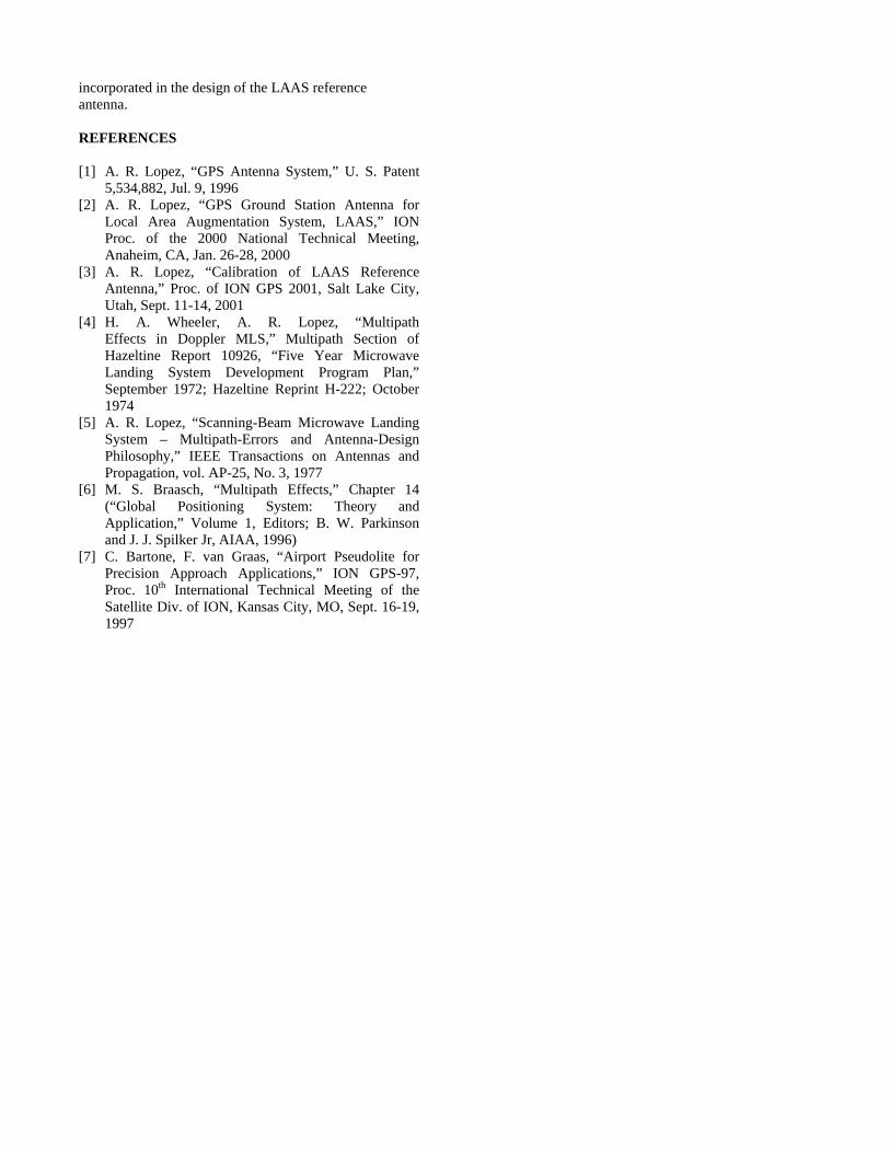
incorporated in the design of the LAAS reference antenna. REFERENCES [1] A. R. Lopez, “GPS Antenna System,” U. S. Patent

5,534,882, Jul. 9, 1996 [2] A. R. Lopez, “GPS Ground Station Antenna for

Local Area Augmentation System, LAAS,” ION Proc. of the 2000 National Technical Meeting, Anaheim, CA, Jan. 26-28, 2000

[3] A. R. Lopez, “Calibration of LAAS Reference Antenna,” Proc. of ION GPS 2001, Salt Lake City, Utah, Sept. 11-14, 2001

[4] H. A. Wheeler, A. R. Lopez, “Multipath Effects in Doppler MLS,” Multipath Section of Hazeltine Report 10926, “Five Year Microwave Landing System Development Program Plan,” September 1972; Hazeltine Reprint H-222; October 1974

[5] A. R. Lopez, “Scanning-Beam Microwave Landing System – Multipath-Errors and Antenna-Design Philosophy,” IEEE Transactions on Antennas and Propagation, vol. AP-25, No. 3, 1977

[6] M. S. Braasch, “Multipath Effects,” Chapter 14 (“Global Positioning System: Theory and Application,” Volume 1, Editors; B. W. Parkinson and J. J. Spilker Jr, AIAA, 1996)

[7] C. Bartone, F. van Graas, “Airport Pseudolite for Precision Approach Applications,” ION GPS-97, Proc. 10th International Technical Meeting of the Satellite Div. of ION, Kansas City, MO, Sept. 16-19, 1997

LAAS Reference Antennas – Key Siting Considerations

Alfred R. Lopez

BAE SYSTEMS

CNIR Division, Antenna Technology Group Greenlawn, NY USA

BIOGRAPHY Alfred R. Lopez is a Life Fellow of the IEEE. He is a Hazeltine Fellow with BAE SYSTEMS Antenna Technology Group. He started his career at Wheeler Laboratories in 1958 as an antenna design specialist. He has made contributions to the theory and practice of electronically scanned antennas. From 1969 to 1990 he was involved with the development of the Microwave Landing System. He has published substantially in IEEE and ION publications, has been issued 39 US Patents, and has received several IEEE and BAE Systems awards. ABSTRACT At the ION Annual Meeting, 2003, a paper [1] was presented, which indicated that lateral multipath was a key issue in the overall performance of the LAAS reference antennas at an airport environment. This paper considers two basic types of lateral multipath objects, fixed and transient, that can significantly affect the LAAS performance. The fixed object is the vertical wall (hangars, terminal buildings) that can cause reflection/diffraction multipath from a vertical wall. The transient objects are an aircraft tailfin and an aircraft fuselage. These transient objects have convex surfaces that generate relatively large specular reflection zones with multipath-to-direct signal ratios that can cause significant multipath error. The goal of this paper is to establish the sensitive zones for these objects. The minimum distance between the reference antenna and the reflecting object will be determined such that the peak multipath error does not exceed a predetermined value. The basic multipath model described in the above referenced paper will be used to quantify the multipath error. In addition, a satellite motion-averaging factor will be considered. The relative motion of the satellite with respect to the earth is such

that, in some cases, the multipath interference frequency is well beyond the pass bands of the code delay-lock-loop and 100-second-average filters, and substantial suppression of multipath error is achieved. INTRODUCTION Lateral multipath is a key issue in the overall performance of the LAAS reference antennas at an airport environment [1]. Lateral multipath includes all airport objects with the exception of the ground. This paper considers two basic types of lateral multipath objects, fixed and transient, that can significantly affect the LAAS performance. The fixed object is the vertical wall (hangars, terminal buildings) that can cause reflection/diffraction multipath from a vertical wall. The transient objects are an aircraft tailfin and an aircraft fuselage. These transient objects have convex surfaces that generate relatively large specular reflection zones with multipath-to-direct signal ratios that can cause significant multipath error. The outline for this paper is presented in Figure 1. After reviewing the general definition of lateral multipath, the general characteristics of a vertical wall, and aircraft tailfins and fuselages are described. The overall LAAS multipath system error is described via a flow diagram, starting with the direct and indirect (multipath) signals, and ending with the system error at the output port of the 100-second-average post filter of the receiver. The concept of multipath satellite motion averaging is described. A critical zone is described as the location of all possible reflectors with delays that are less than 1.05 chips (308 meters). Finally, sensitive zones are described for a vertical wall and the 747 aircraft tailfin. These are the locations for these objects that can possibly cause excessive error.

040922 arl-2

• Airport Multipath• Lateral Multipath – A Significant Problem

—Vertical Wall (Fixed)—Aircraft Tailfin (Transient)—Aircraft Fuselage (Transient)

• LAAS Multipath System Error• Multipath Satellite Motion Averaging• Critical Zone• Sensitive Zone – Vertical Wall• Sensitive Zone – Aircraft Tailfin• Summary

Outline

Figure 1 LATERAL MULTIPATH OBJECTS An overview of airport multipath is presented in Figure 2. In general, lateral multipath is defined as all airport multipath excluding the local ground about the reference antenna. The key lateral multipath objects, with regard to siting considerations for the LAAS reference antennas, are vertical walls, such as hangar walls or hangar doors, and aircraft tailfins and fuselages. Aircraft surfaces are particularly bothersome because they are transient. An aircraft can taxi and park at a location and cause a significant multipath error that could affect more than one of the reference antennas. The net result could be the loss of the availability of a satellite. This would impact the overall system availability.

040922 arl-3

Airport Multipath

• Local Ground• Lateral Multipath

• Hangars• Aircraft Tailfin• Aircraft Fuselage• Airport Control Tower• Terminal Buildings• Buses• Maintenance Vans• Surrounding Skyline

Figure 2 VERTICAL WALL MULTIPATH The basic geometry for the reflection and shadow zones associated with a vertical wall is shown in Figures 3 and 4.

040922 arl-4

Vertical Wall Multipath

ShadowZone

ReflectionZone

Hangar40m Height60m Wide

Ref. Antenna250m from Hangar

0° Az

Figure 3

040922 arl-5

Vertical Wall Multipath (Continued)

-60° -40° -20° 0° 20° 40° 60°

Azimuth Angle

30°

20°

10°

0°

Elev

atio

n A

ngle

Reflection Zone Shadow Zone

Figure 4 Figure 3 is a plan view showing the reflection zone for one wall of the hangar and the shadow zone caused by two walls. Figure 4 shows the possible extent of the reflection and shadow zones in azimuth and elevation angle space.

040922 arl-6

747 Aircraft Tailfin and Fuselage

Figure 5 AIRCRAFT TAILFINS AND FUSELAGES Photographs of a 747 tailfin and fuselage are shown in Figure 5. These are large, mostly convex metal, surfaces that can cause significant multipath over fairly large angular zones. Some typical angular extent of these reflection zones is indicated in Figure 6. (The 747 fuselage actually has a concave reflecting surface at the intersection of the upper deck and the main fuselage. This could significantly enhance the reflection with respect to the reflection of a normally convex surface.)

040922 arl-7

Typical Angular Extent of Reflection Zones

0 to 90±20747 Aircraft Fuselage

5 to 15±15747 Aircraft Tailfin

0 to 10±5Vertical Wall

ElevationAzimuth

Angular Extent(Degrees)

Multipath Object

(Antenna to object distance is 250m. Antenna height above ground is 3m)

Figure 6 LAAS MULTIPATH SYSTEM ERROR A flow diagram for the LAAS multipath system error is presented in Figure 7. The top five layers present an analysis plan for quantifying the multipath-to-direct, M/D, signal ratio. The basic approach for this analysis was developed during the development of the Microwave Landing System [2] [3]. This approach incorporates four

multiplicative factors to provide estimates of the M/D ratio. It should be helpful in supporting the LAAS siting effort, which has been ongoing for several years. [4] [5]. Figure 8 shows some possible factors and the resulting M/D ratios. The receiver processing factor has been characterized by Braasch [6] [7]. Appendix A indicates that -20dB is a representative upper bound for the autocorrelation sidelobe factor. For a 0.1 receiver correlator spacing the total sidelobe multipath suppression factor is 40dB. With a peak raw error of 147m, the sidelobe error at the output of the receiver is 1.5m. Obviously, multipath objects in the sidelobe region need to be considered. Further suppression of multipath error is provided by satellite motion averaging. Figure 9 presents the concept. A multipath source will produce constant phase contours in angle space whose spacing depends on the distance between the multipath source and the reference antenna.

040922 arl-8

LAAS Multipath System Error

Direct Multipath

Size-Curvature Factor

Reflectivity Factor

Polarization Factor

Antenna Gain Difference Factor

Receiver Processing

Delay Lock Loop Filter (BW=0.12 Hz)

Satellite Motion Frequency

100s-Average Post Filter (BW=0.005Hz)

M/D

Envelope of Multipath Error MagnitudeM/D = 0.1 (-20dB)

Correlator Spacing = 0.1

Ref: M. S, Braasch, “Autocorrelation Sidelobe Considerations in the Characterization of Multipath Errors,” IEEE Trans. AES, Vol. 33, No. 1, January 1997

0 200 400 600 8000

0.5

1

1.5

2

Multipath Delay (Meters)

Mul

tipat

h Er

ror M

agni

tude

(Met

ers)

.

Figure 7

040922 arl-9

Example Multipath Factors

0.04 (-27.8dB)0.11 (-19.6dB)0.5 (-6.0dB)M/D

0.70.71Antenna Gain

111Polarization(Linearly Polarized

Ant.)

110.5Reflectivity

0.06110.1511

111111Sizeor

Curvature(Whichever Is Smaller)

Aircraft Fuselage

Hor Vert

Aircraft Tailfin

Hor Vert

Vertical Wall

Hor Vert

Factor

Note: The size-curvature factor is the product of the horizontal and vertical components.

Figure 8

040922 arl-10

Multipath Satellite Motion Averaging

R = 250m

Reference Antenna

MultipathReflector

Angle SpaceConstant Multipath Carrier Phase Contours

θ = λ/Rλ = 0.19mθ = 0.044°θ = 1 cycleSatellite Angular Velocity = ω = 360/(12*60*60) = 0.0083°/s

Satellite Motion Frequency = f (fmax = ω/θ)If satellite moves parallel to contours, then f = 0 HzIf satellite moves perpendicular to contours, then f = 0.19 Hz; Max. Motion Averaging

Figure 9 If the satellite motion is perpendicular to the contour lines, then the multipath signal will have a frequency that is shifted from the carrier frequency. This frequency difference is equal to the satellite angular velocity divided by the angle between the constant phase contours. This frequency shift can be beyond the pass band of the delay-lock-loop filter and well beyond the pass band of the 100-second average post filter. The reduction in the multipath error can be substantial. If the satellite motion is parallel to the constant phase contours, then there is no frequency shift and no corresponding suppression of the multipath error. It is recommended that in a general multipath analysis, the satellite motion averaging factor be set to unity. For site-satellite specific situations, the satellite motion averaging should be quantified. An example is presented later in the paper. THE FRESNEL UNIT OF LENGTH The Fresnel Unit, FU, of length is here defined as

λ= RFU (see Figure 10). In general, the distance, R, is an effective distance that is equal to (R1R2)/(R1 + R2), where R1 is the distance from the antenna to the reflecting object, and R2 is the distance from the reflecting object to the satellite. For the case under consideration, R2 >> R1, and R = R1.

040922 arl-11

The Fresnel Unit Of Length

h WavelengtFreespace Carrier Distance Antennato Reflector Multipath R

R FU Unit Fresnel

=λ=

λ==

If reflecting object size is comparable or larger than FU, then the object has the potential to cause a multipath-to-direct, M/D, ratio near unity (0 dB).If reflecting object is small with respect to FU, then the M/D ratio is less than unity, and the maximum possible M/D ratio is given by the equation:

AreaProjected Reflector A

Ratio) (Voltage FU A

DM

2

=

=

Figure 10 The Fresnel Unit of length serves as a measure of the potential of a reflecting object to cause large or small M/D ratios. As noted in the Figure 10, if the reflecting object size is comparable or larger than the Fresnel Unit, then the object has the potential to cause an M/D ratio near unity. If the reflecting object is small with respect to the Fresnel Unit, then the object will have an M/D ratio that is less than unity. The Fresnel Unit can be used to separate the strong from the weak reflectors. Figure 10 presents an equation that shows the relationship between M/D, reflector projected area, A, and the FU, when the object size is less than the FU. Figure 11 presents a derivation of this equation.

040922 arl-12

Derivation Of Multipath Formula For Small Flat Reflector

20

DirectDirect R4

GPpπ∗

=2

21

212

2

2

21

flectedReflectedRe RR

RRR4

/A4*AR4

GPp ⎥⎦

⎤⎢⎣

⎡++

π

λπ

π

∗=

21

21

RRRRR+

= ( ) 22

2

221

flectedReflectedRe R

ARR4

GPpλ+π

∗=

22

21

0

Direct

flectedRe

Direct

flectedRe

RA

RRR

GG

pp

⎥⎦⎤

⎢⎣⎡

λ⎥⎦

⎤⎢⎣

⎡+

=

λλ=

λλ+==

RH

RW

RA

RA

RRR

GG

VV

DM

21

0

Direct

flectedRe

Direct

flectedRe

Gain FactorDistance Factor

Size Factor

P = Power p = Power Density G = Antenna Gain A = Projected Area

Size Factors:Horizontal

Vertical

Figure 11 In Figure 11, the reflector is a flat perfect electric-conducting plate with a projected square area, A, that is D units on a side. The antenna is in the far-field of the plate.

λ

>λ

>RA

21 or , D2R

2

For the case being considered the gain and distance factors are equal to one. R0 is the direct distance between transmit and receive antennas. For the basic multipath model [1] [2] the reference reflector is a perfect mirror that is tangent to the reflecting object at the point of reflection. The gain and distance factors in Figure 11 correspond to the case of the perfect mirror, an infinitely large, perfect electric-conducting plate.

040922 arl-13

200 100 0 100 200 300

600

500

400

300

200

100

100

200

300

400

500

600

.

Parabola Defines Location of Constant-Delay Multipath

Rπ-φ

Reference Antenna at Parabola Focal Point

Satellite

R(1- cos(φ)) = 300m (Edge of Critical Zone)

Critical ZoneDelay < 308 Meters

Note: Reflecting Surface Is Assumed To Be Tangent To Parabola

))cos(1(RDelay φ−=

Figure 12 THE CRITICAL ZONE The surface of constant delay between two points is an ellipsoid. If one focal point of the ellipsoid is at infinity, then the surface is a paraboloid. For the case of a satellite at a low elevation angle, the intersection of a paraboloid and the ground plane is essentially a parabola. In this paper the critical zone is defined as the location of reflecting objects whose delay is less than 308 meters (1.05 chips). In this zone the receiver processing factor is equal to the correlator spacing. It is -20dB for a correlator spacing of 0.1. Outside of this zone it is typically less than -40dB for the same correlator spacing (see Appendix A). Heretofore [18] it was generally accepted that multipath objects outside the critical zone do not pose a significant threat. In Appendix A, it is shown that the autocorrelation sidelobes are typically more than 20dB down from the peak of the correlation function. In combination with a 0.1 correlator spacing, the total sidelobe suppression of the peak error is 40dB. For the 293m chip, the resulting sidelobe peak error is 1.5m. Clearly, this level of multipath error is not acceptable and must be considered in a site analysis. SENSITIVE ZONE In this paper the sensitive zone is defined as the region surrounding the reference antenna where a particular

multipath source has the potential (size, distance and alignment) to cause an error that exceeds 0.1 meters. Vertical Wall Using the model developed in [2] it is possible to estimate the M/D for the case of the vertical wall. The size factor is the product of horizontal-plane and vertical-plane factors. These size factors are presented in Figure 13.

040922 arl-13

VertHorSize ρρ=ρSize Factor

Size Factor Equations – Vertical Wall

1 Else , Then 1, IfDistance Antennato Reflector R

Angle AzimuthReflector Reflector of WidthW

R)2/sin(W

HorHorHorHor

Hor

=ρρ=ρ<ρ==φ=

λφ

=ρ

1 Else , Then 0, h and 1 If AngleElevation Satellite

Reflector ofHeight H Wallof Edge Top andSight -of-Line Between Distance H)tan(Rh

h2R

VertVertVertVert

Vert

=ρρ=ρ><ρ=θ=

=−θ=πλ

=ρ

Horizontal Size Factor (Reflection at Center of Azimuth Zone)

Vertical Size Factor (Top Edge Reflection/Diffraction)

Figure 13 The horizontal factor corresponds to the M/D at the center of the reflection zone for a vertical strip that has a width equal to W. The vertical factor corresponds to the M/D for a knife edge that has a height above the reference antenna equal to H. The vertical factor varies with the satellite elevation angle. It is noted that the size factor has a sin(φ/2) projected-area dependence (satellite reflection alignment), which has a modified cardioid ( cardioid ) pattern in the azimuth plane.

040922 arl-15

Sensitive Zone Factors – Vertical Wall

0.27 (-11.4dB)0.027 (-31.4dB)Required Size Factor

0.10mMaximum Allowable Error

0.37m3.7mReduced Error

0.25Reflector Reflectivity Factor

0.010.10Receiver Processing Factor

147mMaximum Error

Reflector Location

Inside Outside Critical Zone Critical Zone

Figure 14

040922 arl-16

0 500 1000 1500 2000 2500 3000 3500 4000 4500 500050

45

40

35

30

25

20

15

10

5

0

Horizontal Size FactorVertical Size FactorSize Factor

Antenna-to-Reflector Distance (Meters)

Size

Fac

tor (

dB)

.

Size Factor Along Edge of Critical Zone – Vertical Wall

Satellite Elevation Angle = 5°W = 60mH = 30m

Figure 15

040922 arl-17

1000 500 0 500 1000 1500 2000

500

1000

1500

Critical Zone BoundaryMinimum Distance Outside Critical ZoneMinimum Distance Inside Critical Zone

.

Sensitive Zone – Vertical Wall

A vertical wall, 60m wide and 30m high, should be evaluated withregard to its potential for causing significant multipath error, if it is located inside the parabola, or inside the modified cardioids with radiuses of 400m and 1500m at the intersections with the parabola.

Satellite

1500m

400m

Figure 16 Figure 14 indicates that to satisfy the 0.1m error tolerance the size factor has to be less than -31.4dB inside the critical zone and less than -11.4dB outside the critical zone. Figure 15 shows the variation of the size factor along the boundary of the critical zone. This information is used to map out the edge of the sensitive zone for the vertical wall as shown in Figure 16.

040922 arl-18

Size Factor & Curvature Factor Equations – 747 Tailfin

1 Else , Then ,1 IfDistance Antennato Reflector R

Angle AzimuthReflector Height Reflector H WidthReflector W

RH

R)2/sin(W

SizeSizeSizeSize

Size VertSize Hor

=ρρ=ρ<ρ==φ==

λ=ρ

λφ

=ρ

Curvature of Radius Reflector r)2/sin(r

R21

1Curv

=

φ+

=ρ

Size Factors (Satellite at Center of Reflection Zone)

Horizontal Curvature Factor

Horizontal Size-Curvature Factor

If ρHor Size < ρCurv Then ρHor Size-Curv = ρHor Size Else ρHor Size-Curv = ρ Curv

Figure 17

040922 arl-18

Size-Curvature Equation Validation

0 100 200 300 400 50040

30

20

10

0

Size-Curvature EquationComputer (WIPL) Simulation

Antenna-Reflector Distance (Meters)

Size

-Cru

vatu

re F

acto

r (dB

)

.

W = 2 MetersH = 2 Metersr = 6.7 Metersφ = 90°

Size VerticalCurvature-Size HorizontalCurvature-Size ρρ=ρ

Figure 18 747 Tailfin The tailfin of a 747 aircraft is estimated to be about 9m wide by 9m high. It has curvature in the horizontal plane with a radius of curvature of about 30m [2]. Since it is a metallic surface the reflectivity factor is equal to one. Also, it is assumed that the reference antenna has linear polarization, and consequently, the polarization factor is also equal to one [1]. The size factor and curvature factor equations are presented in Figure 17. The horizontal size and curvature factors are inherently related. The horizontal size-curvature factor is equal to the smaller of the two factors. This relationship was validated using a computer simulation, the results of which are shown in Figure 18

040922 arl-20

Sensitive Zone Factors – 747 Tailfin

0.7Antenna Gain Factor

0.097 (-20.3dB)0.0097 (-40.3dB)Required Size-Curvature Factor

0.10mMaximum Allowable Error

1.03m10.3mReduced Error

1.0Reflector Reflectivity Factor

0.010.10Receiver Processing Factor

147mMaximum Error

Reflector Location

Inside OutsideCritical Zone Critical Zone

Figure 19

040922 arl-20

0 500 1000 1500 2000 2500 3000 3500 4000 4500 500050

45

40

35

30

25

20

15

10

5

0

Vertical Size FactorHorizontal Size and Curvature FactorSize-Curvature Factor


Size

Cur

vatu

re F

acto

rs (d

B)

.

Size-Curvature Factor Along Edge of Critical Zone –747 Tailfin

Tailfin:Width = 9mHeight = 9mRadius of Curvature = 30m

Figure 20

040922 arl-22

1500 1000 500 0 500 1000 1500 2000 2500 3000 3500 4000

500

1000

1500

2000

Critical Zone BoundaryMinimum Distance Outside Critical ZoneMinimum Distance Inside Critical Zone

.

Sensitive Zone – 747 Tailfin

A 747 tailfin should be evaluated with regard to its potential for causing significant multipath error, if it is located inside the parabola or inside the modified cardioids with radiuses of 550m,and 3700m at the intersections with the parabola.

Satellite

3700m

550m

Figure 21 In Figure 18 the geometry was set such that the curvature factor was the smaller of the two factors. Computer simulations were also run for the cases when the size

factor was the smaller of the two and when they were about equal. In all cases there was good agreement between the equations of Figure 17 and the computer simulations. Figure 19 indicates that to satisfy the 0.1m error tolerance the tailfin size-curvature factor has to be less than -40.3dB inside the critical zone and less than -20.3dB outside the critical zone. Figure 20 shows the variation of the size-curvature factor along the boundary of the critical zone. This information is used to map out the edge of the sensitive zone for the tailfin as shown in Figure 21. POLARIZATION AND MOTION AVERAGING FACTORS The indicated sensitive zones for the vertical wall and aircraft tailfin are very large, and in many cases, would seriously impact the siting of reference antennas. As noted in [1], a reference antenna with right hand circular polarization with an axial ratio of 2 dB would provide about another 20 dB reduction of the M/D ratio. This would greatly reduce the size of the sensitive zones. It is noted that the satellite motion frequency depends directly on the separation distance, R, between the antenna and the reflecting object and, consequently, increased satellite-motion-averaging suppression of multipath error is directly related to the separation distance. An example is presented below that illustrates the multipath suppression related to satellite motion averaging. It is assumed that the satellite angular velocity component perpendicular to the multipath constant-phase contours is one half the satellite angular velocity, and the spacing of the contours is twice the minimum spacing. The frequency dependence on R is given by the equation:

λπ

=R

)60)(60(122

41)R(f (Hz)

The phase lock loop filter is assumed to be a low-pass single-pole filter with a pass-band frequency, f1 = 0.12 Hz. The filter response, F1(R), is approximated by:

1)R(F Else ,)R(f

f)R(F Then ,1)R(f

fIf 11

11 ==<

The 100s averaging filter is assumed to be a low-pass single-pole filter with a pass-band frequency, f2 = 0.005 Hz. The filter response, F2(R), is approximated by:

1)R(F Else ,)R(f

f)R(F Then ,1)R(f

fIf 22

22 ==<

Figure 22 presents the size-motion multipath suppression factor along the critical zone perimeter. As compared with Figure 16, Figure 23 indicates that with the satellite

motion averaging factor included the sensitive zone is greatly reduced. In Figure 23 the sensitive zone is bounded by the critical zone parabola and a modified cardioid with a 400m-radius at the intersection with the parabola.

040922 arl-23

0 500 1000 1500 2000 2500 3000 3500 4000 4500 500050

45

40

35

30

25

20

15

10

5

0

Size FactorMotion Filter FactorMotion Filter and Size Factor


Size

-Mot

ion

Fact

or (d

B)

.

Size-Motion Factor Along Edge of Critical Zone – Vertical Wall

Satellite Elevation Angle = 5°W = 60mH = 30m

Figure 22

040922 arl-24

200 100 0 100 200 300 400

100

200

300

400

500

600

Critical Zone BoundaryMinimum Distance Inside Critical Zone

.

Sensitive Zone – Vertical Wall –Satellite Motion Factor Included

Satellite

In this case the sensitive zone is bounded by the critical zone perimeter and a modified cardioid with a 400m radius at the intersection of the parabola.

400m

Figure 23 MATH MODELING The airport environment is complicated and varied, so much so, that no one particular math model is useful in all situations. Specially designed software [5] and commercially available software packages can be used to accurately predict M/D and, receiver processing and filtering. These models are generally more useful for either the case when the object is electrically large or when the object is electrically small. In all cases, the math models can not typically accommodate all of the features of the airport objects and, consequently, there is some residual error in the performance predictions.

The model originally developed in [2], and further refined in [1] and in this paper, is universally applicable to large and small objects. It is based on analysis and the decomposition of the problem to its basic elements. It provides insight into the phenomena that affect the M/D ratio. It also provides a relatively simple way for estimating peak M/D ratios. One particularly useful feature of this simple model is the curvature factor, which provides a way of quickly estimating the magnitude of reflections off convex aircraft surfaces. The curvature factor defined in [2] was first derived by Riblet and Barker [9] as a divergence factor for a doubly curved surface. The author converted their results to the form presented in Figure Q-13 (a) of [2], where the reference reflector is a perfect electric mirror. A siting engineer will need all of the tools available. A siting handbook should incorporate computer software packages, both custom and commercial, and the concepts and methodology described in this paper. SUMMARY • Vertical walls, aircraft tailfins and aircraft fuselages

have been identified as key multipath sources that need special consideration in the siting of the LAAS reference antennas.

• Multipath satellite motion averaging was described. It is very effective in suppressing multipath error however it is recommended that the basic analysis be performed independent of the motion averaging factor. This will provide insight into the basic error mechanism.

• A critical zone was defined as the region around the reference antenna were the multipath delays are less than 1.05 chips, 308 meters. A parabola defines the outer boundary of this region.

• A sensitive zone was defined as a region where lateral multipath objects have the potential to cause excessive error. The sensitive zones for a vertical wall and a 747 aircraft tailfin were evaluated.

• The goal was to introduce a relatively simple methodology for quantifying the potential threat associated with common airport multipath sources.

ACKNOWLEDGEMENTS The author would like to thank Dr. Michael S. Braasch, of Ohio University, for his help in characterizing the autocorrelation sidelobe factor and for his general encouragement of the work reported in this paper. APPENDIX A – Autocorrelation Sidelobe Factor Via [10] the following data (PRN Number, Sidelobe Error Factor) were provided:

(1, 0.0) (2, 0.0625) (3, 0.0625) (4, 0.0625) (5, 0.0) (6, 0.0625) (7, 0.0667) (8, 0.1176) (9, 0.0625) (10, 0.0625) (11, 0.0625) (12, 0.0) (13, 0.0625) (14, 0.0) (15, 0.0667) (16, 0.0625) (17, 0.0667) (18, 0.1250) (19, 0.1250) (20, 0.0625) (21, 0.0667) (22, 0.0588) (23, 0.0625) (24, 0.1333) (25, 0.1250) (26, 0.0) (27, 0.0625) (28, 0.0625) (29, 0.0) (30, 0.1250) (31, 0.0) (32, 0.0) This data has the following characteristics: Maximum Value = 0.1333 (-17.5 dB) Mean Value = 0.0590 (-24.6 dB) Standard Deviation = 0.0420 (-27.5 dB) Root Mean Square Value = 0.0721 (-22.8 dB) Mean + Standard Deviation = 0.1010 (-19.9 dB) The mean value plus the standard deviation (-20 dB) is a value that is not exceeded more than 16 percent of the time, and is used in this paper as representative of the upper bound for the autocorrelation sidelobe factor. REFERENCES [1] A. R. Lopez, “LAAS Reference Antennas – Circular

Polarization Mitigates Multipath Effects,” Proc. Of ION Annual Meeting, Albuquerque, NM, June 23-25, 2003

[2] H. A. Wheeler, A. R. Lopez, “Multipath Effects in Doppler MLS,” Multipath Section of Hazeltine Report 10926, “Five Year Microwave Landing System Development Program Plan,” September 1972; Hazeltine Reprint H-222; October 1974.

[3] A. R. Lopez, “Scanning-Beam Microwave Landing System – Multipath-Errors and Antenna-Design Philosophy,” IEEE Transaction on Antennas and Propagation, vol. AP-25, No. 3, 1977

[4] D. Lamb, “Development of Local Area Augmentation System Siting Criteria,” ION 57th Annual Meeting/CITGTF 20th Biennial Guidance Test Symposium, 11-13 June 2001, Albuquerque, NM.

[5] J. M. Kelly, J.C. Cohenour, M. F. DiBenedetto, D. Lamb, “An Advanced Multipath Model for DGPS Reference Site Analysis,” ION 60th Annual Meeting, June 7-9, 2004, Dayton, OH.

[6] M. S. Braasch, “Autocorrelation Sidelobes Considerations in the Characterization of Multipath Errors,” IEEE Trans. AES, Vol. 33, No. 1, January 1997

[7] M. S. Braasch, M. F. DiBenedetto, “Spread-Spectrum Ranging Multipath Model Validation,” IEEE Trans. AES, Vol. 37, No. 1 January 2001

[8] D. B Thornberg, D. S. Thornberg, M. F. DiBenedetto, M. S. Braasch, F. van Graas, C. Bartone, “LAAS Integrated Multipath-Limiting

Antenna,” Navigation, ION Journal, Vol. 50, No. 2, Summer 2003.

[9] H. J. Riblet, C. B. Barker, “A General Divergence Formula,” Journal of Applied Physics, Vol. 19 pp. 63-70, January 1948.

[10] M. S. Braasch, Email correspondence, August 7, 2004.

LAAS/GBAS Ground Reference Antenna With

Enhanced Mitigation of Ground Multipath

Alfred R. Lopez, BAE Systems

BIOGRAPHY Alfred R. Lopez is a Life Fellow of the IEEE. He is a Hazeltine Fellow and Engineering Fellow with BAE Systems, Greenlawn, NY. He started his career at Wheeler Laboratories in 1958 as an antenna design specialist. He has made contributions to the theory and practice of electronic scanned antennas. From 1969 to 1990 he was involved with the development of the Microwave Landing System. He has published extensively in IEEE publications, has been issued 46 US Patents, and has received several IEEE and BAE Systems awards. He is the inventor of the ARL-1900 Ground Reference Antenna. ABSTRACT The concept for the ARL-1900 LAAS/GBAS ground reference antenna was first described at the ION 2000 National Technical Meeting. This antenna has the following features: • One-port circular-polarization L1-L2-L5 coverage of

the upper hemisphere • Sharp antenna pattern cutoff on the horizon for

mitigation of ground multipath at low elevation angles

• 30 dB sidelobes in the lower hemisphere for mitigation of ground multipath at higher elevation angles

• Very high quality carrier delay (antenna phase center) and code (group) delay characteristics

• Circular polarization at low elevation angles for mitigation of lateral multipath

This antenna has been under development since 1999, and is now entering the initial phase of field deployment. The prototype ARL-1900 antenna was built under contract to the FAA. After successful testing by the FAA, in December of 2005, 17 additional antennas were built and tested. Ten additional antennas are currently being built.

This paper reviews the ground multipath issue and describes a means for enhanced mitigation of the ground multipath problem. The variability of the ground reflectivity is quantified and its impact on the possible variation of the ground multipath error is described. Siting recommendations are made which enhance the multipath performance INTRODUCTION The ARL-1900 ground reference antenna is shown in Figure 1 installed at the William J. Hughes FAA Technical Center, Atlantic City, NJ. It is a 19-element collinear array antenna designed specifically for the LAAS/GBAS application. Figure 2 shows the array antenna with the radome removed.

ARL-1900 Differential GPS Ground Reference Antenna

0

30

6090

120

150

180

210

240270

300

330

4035302520151050

.

COMPUTER SIMULATION

MEASUREMENT

Figure 1

ARL-1900 Antenna – Radome Removed

19 Element Array9 Excited Elements

10 Parasitic ElementsHigh-Accuracy Array Excitation

(±0.25 dB, ±2º)

Figure 2 The array antenna comprises 19 radiating elements and a 9-way-power-divider and cabling assembly as shown in Figure 2. The cabling assembly has 9 equal-length coaxial cables that connect to (counting from the bottom) elements numbers 3, 5, 7, 9, 10, 11, 13, 15, and 17. These elements are excited directly; the remaining elements are excited parasitically (indirectly via mutual coupling).The ARL-1900 is a very simple but a very high precision antenna. The key features of the ARL-1900 antenna are: • One-port, circular polarization, L1-L2-L5 coverage

of the upper hemisphere o One port – one receiver, no satellite handover

problem o Full GNSS band, 1150-1600 MHz

• Sharp antenna pattern cutoff on the horizon for mitigation of ground multipath at low elevation angles o 2.5 dB/º slope on horizon o 30 dB antenna Up/Down gain ratio down to 6º

elevation • 30 dB sidelobes in the lower hemisphere for

mitigation of ground multipath at higher elevation angles o 30 dB antenna Up/Down gain ratio

• Very high quality carrier delay (antenna phase center) and code (group) delay characteristics o Carrier delay variation ±1cm (unit-to-unit ±1mm) o Code delay variation ±2.5cm (unit-to-unit ±3mm)

• Circular polarization at low elevation angles for mitigation of lateral multipath [5-6] o Taxing aircraft, hangers, etc.

• Unit-to-unit de-correlated sidelobes in the lower hemisphere o Enhances ground multipath de-correlation amongst

ground reference receivers • Integral air terminal for lightning protection

o Non-scattering air terminal configuration, no performance degradation

The initial concept for the ARL-1900 was developed in 1993 and the first patent was issued in 1996 [1]. The initial concept was very narrow band and there were problems with the implementation. An improved wideband version was developed in 1999 with an associated patent issued in 2001 [2]. This second version had the same basic architecture as the ARL-1900 [3] but it had one significant problem, excessive code delay variation with azimuth angle at high elevation angles [4]. The solution to the problem associated with the second version became apparent in 2003. The ARL-1900 antenna is the embodiment of this solution. Measurements in December of 2005, at the William J. Hughes FAA Technical Center [7] (see Figure 3) demonstrated excellent performance for the ARL-1900 antenna. FAA Measurement – Atlantic City – December 17, 2005

ARL-1900 Antenna – Serial No. 001

Figure 3 RANDOM SIDELOBES ENHANCE MULTIPATH DE-CORRELATION AMONGST REFERENCE RECIEVER STATIONS The requirement for coverage of the upper hemisphere results in an inherently low-gain antenna. Ideally, with no antenna dissipative loss, the highest gain possible is 3 dBi. It is very difficult to design a low-gain antenna with low sidelobes (30 dB). The design strategy for achieving low sidelobes for a low gain antenna was presented in [3]. The basic concept is to set the systematic (zero array-excitation error) peak sidelobe level substantially below the desired peak sidelobe level (30 dB), and then to specify the error tolerance on the array excitation such that the combined 2-sigma value for the peak systematic and error sidelobes is less than 30 dB. Figure 4 presents the basic approach for the design of the ARL-1900 antenna. The array excitation tolerances of ± 0.2 dB and ± 2º require high precision components for the collinear array antenna. The elevation patterns for 20 random-error trials presented in Figure 4 show the predominant random nature of the unit-to-unit sidelobe levels

ARL-1900 Random Sidelobe level

Random sidelobelevels with 0.2 dB amplitude and 2°phase errors

2-sigma up/down gain ratio equals 29.6 dB

Zero ErrorPeak Sidelobe Level

One significant benefit for the ARL-1900 antenna is provided by the random nature of the unit-to-unit sidelobe level. Four reference receiver stations are typically utilized to suppress multipath. The four stations are located with respect to each other to provide de-correlation of the multipath signals. The random nature of the ARL-1900 antenna unit-to-unit sidelobe level enhances the de-correlation of the ground multipath signals.


Figure 4

GROUND MULTIPATH CHARACTERISTICS The basic geometry for ground multipath is shown in Figure 5. At the antenna phase center the direct signal and a ground reflected (multipath) signal are combined. The polarization of the ground reflected signal experiences a transformation upon reflection. The Fresnel formulas quantify this transformation and are presented below.

Ground Multipath Geometry

Delay = 2 H sin( θ )

θ

Antenna Phase Center

HGround Reflected

(Fresnel Formulas)

Direct

Figure 5 The Fresnel formulas for the reflection factor for vertical polarization, ΓVP, and for horizontal polarization, ΓHP, are given by:

angle Elevation frequency Radian

tyConductivi constant dielectric Relative

constant dielectric space Free

)(cosj)sin(

)(cosj)sin(

)(

)(cosj)sin(j

)(cosj)sin(j

)(

r

0

2

0r

2

0r

HP

2

0r

0r

2

0r

0r

VP

=θ=ω=σ=ε

=ε

θ−⎟⎟⎠

⎞⎜⎜⎝

⎛ωεσ

−ε+θ

θ−⎟⎟⎠

⎞⎜⎜⎝

⎛ωεσ

−ε−θ

=θΓ

θ−⎟⎟⎠

⎞⎜⎜⎝

⎛ωεσ

−ε+θ⎟⎟⎠

⎞⎜⎜⎝

⎛ωεσ

−ε

θ−⎟⎟⎠

⎞⎜⎜⎝

⎛ωεσ

−ε−θ⎟⎟⎠

⎞⎜⎜⎝

⎛ωεσ

−ε

=θΓ

Ground Parameters

481Smooth Sea

0.0014Very Dry Ground

0.00216Wet Ground

0.0181Fresh Water

Conductivity, σ(S/m)

Relative Dielectric Constant, εr

Ground Type

Figure 6

Ground Reflection Factor – Linear Polarization

0 10 20 30 40 50 60 70 80 900

0.1

0.2

0.3

0.4

0.5

0.6

0.7

0.8

0.9

1

Smooth Sea Vertical PolarizationSmooth Sea Horizontal PolarizationVery Wet Ground Vertical PolarizationVery Wet Ground Horizontal PolarizationVery Dry Ground Vertical PolarizationVery Dry Ground Horizontal Polarization

Ref

lect

ion

Fact

or (V

olta

ge R

atio

)

.Brewster Angle: Elevation angle where the vertical polarization component is a minimum value

Frequency = 1575 MHz

Figure 7 The ground reflection characteristics are quantified by two parameters in the Fresnel formulas, the relative dielectric constant, εr and the conductivity, σ. Figure 6 presents a table that lists these parameters for four different types of grounds ranging from a smooth sea to a very dry ground.

Ground Reflection Factor – Circular Polarization

0 10 20 30 40 50 60 70 80 9010

9

8

7

6

5

4

3

2

1

0

Smooth Sea Circular PolarizationVery Wet Ground Circular PolarizationVery Dry Ground Circular Polarization


Circ

ular

Pol

. Ref

lect

ed P

ower

(dB

)

.

≈ 8 dB

H = 3m, Antenna Up/Down Gain Ratio = 30 dB δ = 15 cm

δ = 6 cm

δ = 11 cm

MultipathError

Figure 8 The reflection factor magnitude versus elevation angle for vertical and horizontal linear polarization components of an incident signal are presented in Figure 7. The Brewster angle is defined as the elevation angle where the magnitude of the vertically polarized component is a minimum. The reflection phase for the vertically polarized component varies 180º across the Brewster angle. The handedness for a reflected circularly polarized incident signal reverses across the Brewster angle. On the zenith side of the Brewster angle an incident right-hand circularly polarized incident signal is reflected with left-hand polarization. Figure 8 presents the magnitude of the reflection factor for an incident circularly polarized signal. At angles near the horizon right hand circular polarization is reflected as right-hand circular polarization. At the Brewster angle the reflected signal is essentially horizontally polarized. At angles near zenith, an incident signal with right-hand circular polarization is reflected with left-hand circular polarization. (There have been cases where the antenna gain pattern has been measured with respect to right hand circular polarization, and the ratio of the gain in the zenith direction to the gain in the nadir direction has been reported as the desired-to-undesired ratio for the zenith direction. This, of course, was in error since the antenna has, inherently, left-hand circular polarization in the nadir direction.) Figure 8 shows that for elevation angles below 10º the magnitude of the reflection factor is essentially independent of the type of ground. For elevation angles above 30º there is substantial variation of the reflection factor magnitude. In the zenith direction there can be an 8 dB difference in the reflection magnitude for smooth sea and a very dry ground. The corresponding variation in the multipath error could range from 15 cm for the case of a smooth sea to 6 cm for the case of very dry ground.

DEFINITION OF DESIRED-TO-UNDESIRED (D/U) SIGNAL RATIO For a given satellite elevation angle and assuming a flat horizontal ground: The D/U ratio is defined as the ratio of the received direct signal to the received multipath (indirect) signal. An approximate formula for D/U is given by:

)()(Ratio Gain Down/Up

)(1

)(G)(G)(

UD

θΓθ

=θΓθ−

θ≈θ (1)

G(θ) = Antenna gain with respect to an isotropic antenna (dBi, total radiated power) Γ(θ) = Magnitude of ground reflection factor θ = Elevation angle Equation (1) assumes polarization match for both the direct and indirect signals. (The magnitude of the direct signal is proportional to the total power in the direct signal; the magnitude of the indirect signal is proportional to the total power in the reflected signal.) It is a conservative estimate for the D/U ratio. An exact formula for D/U is given by:

onpolarizati horizontal for formula Fresnel onpolarizati vertical for formula Fresnel

onpolarizati linear horizontal to respect withgain AntennaG

onpolarizati linear vertical to respect withgain AntennaG

(2) )()(jG)()(G

)(jG)(G)(

UD

HP

VP

HP

VP

HPHPVPVP

HPVP

=Γ

=Γ

=

=

θΓθ−+θΓθ−θ+θ

=θ

All the factors in Equation (2) are complex voltages. MULTIPATH ERROR VERSUS ELEVATION ANGLE The multipath error, δ(θ), versus elevation angle is given by the approximate formula [8]:

⎟⎠

⎞⎜⎝

⎛ θλπ

θθΓθθ−

≈θδ

⎟⎠

⎞⎜⎝

⎛ θλπ

θθ

≈θδ

)sin(H4sin)sin(H2)()(G)(G)(

)sin(H4sin)sin(H2)(U/D

1)( (3)

It is assumed that the ground is flat and horizontal. Equation (3) is valid for H < 7.5 m and D/U >> 1.

Multipath Error Versus Elevation Angle

0 10 20 30 40 50 60 70 80 900.2

0.1

0

0.1

0.2


Cod

e D

elay

Mul

tipta

h Er

ror (

Met

ers)

.

H = 3 mD/U(θ) = 36 dB = Antenna Up/DownGainRatio/Γ(θ)Antenna Up/DownGainRatio = 30 dBΓ(θ) = - 6 dB

Figure 9 Multipath error versus elevation angle is presented in Figure 9. The interference pattern shown in Figure 9 is simply that of a source located 3 m above the ground surface and its image 3 m below the surface. It is noted that if the antenna were located above a pool of water, the peak error would be near 0.15 m. GENERAL SITING CONSIDERATIONS As indicated in Equation (3), the peak multipath error is directly related to the antenna height above the local ground. One would tend to locate the antenna as close to ground as possible, but it is soon recognized that this location would be overly sensitive to local transient objects that can produce substantial multipath effects. Experience to date has indicated that an antenna phase center height of 3 m is suitable for airport environments. It is recommended that the phase center height should not be less than 2 m. The variability of the peak multipath error associated with the water content of the local ground leads to the following recommendations: • Avoid a site with a local bowl-shaped (concave)

terrain feature • Concave ground can amplify the ground

reflection factor • Concave ground can also accumulate rain water

at the base of the antenna • Location at the apex of a convex surface is the

ideal location • Stabilization considerations

• Grade the local site (4 m radius) to minimize the possibility of a water saturated local ground or pools of water near the antenna base

• Add a layer of crushed stone (or other suitable materials) to provide a stable electrically-rough surface with a reflection factor ranging between -6 and -9 dB

SUMMARY This paper: • Presented an overview of the ARL-1900 ground

reference antenna performance and history. This antenna is unique with near ideal characteristics

• Presented a detailed description of ground multipath characteristics, which highlighted the possible variability of the local ground reflectivity. This impacts the multipath performance, especially at high elevation angles

• Made recommendations for the siting of the antenna and possible treatment of the local ground surface for control of the variability of the local ground reflectivity

ACKNOWLEDGEMENTS Many thanks are given to Mr. John Warburton (William J. Hughes FAA Technical Center) for his help over the many years with the development of the ARL-1900 antenna. The successful development of the ARL-1900 antenna is credited, in great part, to the technical leadership of Mr. Gary A. Schay (BAE Systems) and the managerial leadership of Mr. Gary T. Nolan (BAE Systems). REFERENCES [1] A.R. Lopez, U.S. Patent No. 5,534,882, “GPS

Antenna Systems,” Jul. 9, 1996 [2] A.R. Lopez, R.J. Kumpfbeck, E.M. Newman, U.S.

Patent No. 6,201,510, “Self-Contained Progressive-Phase GPS Elements and Antennas,” Mar. 13, 2001

[3] A.R. Lopez, “GPS Ground Station Antenna for Local Area Augmentation System, LAAS,” ION NTM 2000, 26-28 January 2000, Anaheim, CA

[4] A.R. Lopez, “Calibration of LAAS Reference Antennas,” ION GPS 2001, 11-14 September 2001, Salt Lake City, UT

[5] A.R. Lopez, “LAAS Reference Antennas – Circular Polarization Mitigates Multipath Effects,” ION 59th Annual Meeting/CIGTF 22nd Guidance Test Symposium, 23-25 June 2003, Albuquerque, NM

[6] A.R. Lopez, “LAAS Reference Antennas – Key Siting Considerations,” ION GNSS 17th International Meeting of the Satellite Division, 21-24 Sept. 2004, Long Beach, CA

[7] FAA Navigation/LAAS T&E Team, “Local Area Augmentation System Performance Analysis / Activities Report, Report #9, Reporting Period: January 1 to March 31, 2006,” April 30, 2006, pp. 43-45

[8] C.C. Counselman, “Multipath-Rejecting GPS Antennas,” Proceedings of the IEEE, Vol. 87, No. 1, Jan 1999

bae systems arl-1900 antenna laas/gbas ground …arlassociates.net/baesystemsarl-1900antenna.pdfbae...

Documents