background and anthropogenic influences on … and anthropogenic influences on atmospheric co 2...

Boreal environment research 20: 213–226 © 2015issn 1239-6095 (print) issn 1797-2469 (online) helsinki 30 april 2015

Editor in charge of this article: Veli-Matti Kerminen

Background and anthropogenic influences on atmospheric co2 concentrations measured at Pallas: comparison of two models for tracing air mass history

Tuula Aalto, Juha Hatakka, Rostislav Kouznetsov and Karolina Stanislawska

Finnish Meteorological Institute, P.O. Box 503, FI-00101 Helsinki, Finland

Received 2 Dec. 2013, final version received 8 Oct. 2014, accepted 10 Oct. 2014

Aalto T., Hatakka J., Kouznetsov R. & Stanislawska K. 2015: Background and anthropogenic influences on atmospheric CO2 concentrations measured at Pallas: Comparison of two models for tracing air mass history. Boreal Env. Res. 20: 213–226.

The FLEXTRA and SILAM models were utilized in estimating the influence regions (IR) for the measured CO2 concentration ([CO2]) at Pallas together with tracers for anthro-pogenic emissions. The models produced similar synoptic features and associated back-ground [CO2] with marine IR and elevated [CO2] with continental IR, but there were also differences which affected the interpretation of measurements. The background, i.e. marine boundary layer (MBL) signal, was compared to the NOAA MBL reference. Both models performed well, with monthly mean deviations from the reference usually inside 1 ppm. The FLEXTRA MBL signal had some seasonality in the difference, however, only very few cases were associated with anthropogenic emissions. We used [CO] and fossil fuel [CO2] simulations by the TM5 (CarbonTracker CT2011_oi) model as emission tracers. The model and [CO] captured well the timing of high [CO2] in measurements. The anthropo-genic influence was more pronounced in winter than in summer, and it had a large inter-an-nual variation.

Introduction

Remote areas are quite different in their annual cycle of the carbon dioxide concentration, [CO2], in comparison with large cities, where anthro-pogenic sources are always present. CO2 is a long-lived gas, and it has a certain background concentration, i.e. historical residue of emit-ted CO2 that still remains in the atmosphere. Some anthropogenic emissions are freshly brought to remote stations and are clearly distin-guishable from the background, while majority of the emissions are well mixed in the atmo-sphere before measurements. Distinguishing the background signal from the measurements

is a challenge, especially if the measurements are made in a low-altitude continental location (Thompson et al. 2009, Vermeulen et al. 2011). A local influence is often visible when atmo-spheric mixing is weak. Thus measurements are usually filtered by e.g. removing periods with low wind speed and high standard deviation in hourly mean concentrations (Thoning et al. 1989, Bousquet et al. 1996). Tracking the history of air masses provides information about distant regions that affect the measured concentration level. If air masses were transported at low alti-tudes over continental, populated regions before their arrival at the measurement station, we can expect higher [CO2] levels than after transport

214 Aalto et al. • Boreal env. res. vol. 20

above a marine region (e.g. Biraud et al. 2000). Knowledge of air mass history is especially important if a global background concentration or a marine boundary layer (MBL) signal is studied. The global composite of multi-site MBL reference is regularly reported by NOAA/ESRL (GLOBALVIEW-CO2, 2011, http://www.esrl.noaa.gov/gmd/ccgg/mbl/index.html), allowing comparisons with individual site measurements.

The measured [CO2] level depends on the air mass history (e.g. Aalto et al. 2002, Eneroth et al. 2005), and there are different methods to trace this quantity. Traditionally, a Lagrangian trajectory model has been used, which gives only one back-trajectory path related to one measurement time and place. Measurements have the maximum sensitivity to sources located along the path, i.e. sources located on the trajec-tory path affect the measurement stronger than sources away from it. A single trajectory does not provide information on how sensitive the measurement is to the sources away of it, since it does not account for mixing. To overcome this difficulty, an ensemble of trajectories with random walk can be used to simulate mixing. The density of trajectories gives the sensitivity pattern or footprint. An accurate evaluation of the footprint requires very large number of tra-jectories. Alternatively, an Eulerian dispersion model can be run to evaluate the footprints. In this work, the Lagrangian trajectory model FLEXTRA (Stohl et al. 1995, Stohl and Seibert, 1998) and Eulerian dispersion model SILAM (Sofiev et al. 2006, Sofiev et al. 2008) are com-pared from a perspective of selecting Pallas [CO2] measurements according to different source regions.

In studying the anthropogenic sources of CO2, other concurrently-monitored tracers can be utilized that are more strongly associated with anthropogenic emissions. Traffic is a source of both CO2 and CO (Olivier et al. 2005, Granier et al. 2011, see also Pommier et al. 2013). Nat-ural sources of CO (fires, volcanoes) are often non-significant contrary to those of CO2, and thus [CO] can be used as a tracer of anthropo-genic [CO2]. During dark and cold winter con-ditions, the atmospheric lifetime of CO is long enough so that remote areas can be affected by anthropogenic CO2 and CO pollution. There are

also other good tracers of anthropogenic influ-ence like isotopic signature of [CO2] (namely ratio of 14C/12C in measured [CO2], Vogel et al. 2010, 2013), but multi-year time series of 14C measurements are available from only a limited number of sites.

Map-based information on CO2 sources and sinks together with an atmospheric transport model can be used to simulate concentrations at individual measurement sites (e.g. Geels et al. 2004, Peters et al. 2010). The simulated concen-trations can be marked for contributions coming from anthropogenic, biogenic, fire and oceanic sources. The modeled anthropogenic contribu-tion, together with [CO], can be used to explain the variation in measured [CO2] due to rela-tively recent pollution sources. One aim of the SNOWCARBO project, the outcome of which is presented in this special issue, was to assess the anthropogenic contribution to measured CO2 concentrations. In order to do it, we also ought to define the baseline in [CO2]. In this study, a re-assessment of the baseline conditions is given together with discussion about fresh anthropo-genic influences in measured [CO2]. We also studied the connections between the anthropo-genic episodes and continental and marine influ-ence regions.

Material and methods

Site and measurements

The Pallas site is located in the Pallas-Yllästun-turi National Park in northern Finland (Hatakka et al. 2003, Aalto et al. 2002). The region is sparsely populated and relatively unpolluted, as the nearest population center of 2500 inhab-itants is located at a distance of 19 km. The main station, Sammaltunturi, is located on the treeless top of a hill (67°58´24´´N, 24°06´58´´E, 565 m a.s.l.). The terrain around the site is covered by patches of boreal forests, wetlands and lakes. The lowest winter temperatures may drop below –30 °C, while the highest summer temperatures rise above 20 °C. The ground is covered with snow usually from October to May. Since the area is located above the Arctic Circle, in December–January there is a period when

Boreal env. res. vol. 20 • Background and anthropogenic influences on CO2 at Pallas 215

the sun is continuously below the horizon. The summer insolation is correspondingly high, with a period of 24-hour daylight in June–July.

CO2 and CO concentrations are continuously monitored at the site. For CO2, a nondispersive infrared (NDIR) based system had been in use until 2010, thereafter the system was based on a cavity ring down spectroscopy (CRDS) instru-mentation. At the station, the air was pumped at a rate of ca. 130 m3 hour–1 through a stainless-steel manifold system. All the instruments measuring gaseous components take their sample air from this manifold. Before entering the NDIR instru-ment, the sampled air was dried with a cryogenic cooler (–30 °C) and chemical desiccant (Magen-sium perchlorate). For the CRDS instrument, a nafion dryer (Perma Pure MD-070-96S-2) was used. The NDIR setup included three work-ing standards, reference gas and target cylinder, and the CRDS setup had one target cylinder. The instruments and cylinders were calibrated against a set of seven WMO/CCL standard refer-ence gases (scale WMO CO2 X 2007) four to six times a year.

CO mixing ratios were measured four times an hour with an automated gas chromatographic system (Agilent 6890N) equipped with a flame ionization detector (FID and a methanizer. The calibration of the measured signal was made with a working standard by measuring it as every other sample. The working standard was cali-brated against a set of three WMO/CCL standard reference gases (scale WMO CH4 X 2004) four to six times a year. The [CO] measurement is not fully validated for precise monitoring of long-term [CO] levels, yet it is adequate for detecting episodes due to anthropogenic emissions.

Data selection and NOAA MBL data product

In order to remove periods with weak atmo-spheric mixing and thus significant local influ-ences, the hours with a low wind speed and high concentration variation were excluded from the [CO2] data set. Based on wind statistics, during June–August, the limit was 3 m s–1 and during the rest of the year 4 m s–1. The limit for 1 SD in hourly concentrations was 0.5 ppm in summer

and 0.3 ppm in winter. Together, these conditions excluded about 30% of the data. The same wind limits were applied to CO concentration data.

The CO2 concentration increased from year to year and had a strong annual cycle. A func-tion consisting of a third order polynomial for the growth rate and four harmonic terms for the annual cycle was fitted to the non-local data and the residuals were filtered according to the widely used methods by Thoning et al. (1989). This procedure served different purposes: (1) Additional constraint for the use of measure-ments in MBL selection was set by evaluating the distance of CO2 concentrations to fit. In order to be included in the MBL data set, excep-tionally high or low values (> 2.0 SD from the fit) were removed. (2) Deviation from the fit towards higher concentrations was utilized in determining if the measured signal was affected by anthropogenic pollution. (3) Removing the growth trend enabled comparisons of the annual cycle in different years.

The Pallas site is located in northern boreal zone with distinct natural forest, soil and wetland GHG sinks and sources, but it is also under the influence of air masses transported from north-ern–western marine or southern–eastern conti-nental populated and industrialized areas. The surroundings of Pallas were divided into five influence regions (IR), as presented by Aalto et al. (2002), bounded by latitude and longitude: “Local” included continental northern Finland, Sweden and Norway, “Arctic” included north of 71°N, “East” extended east from 29°E, “West” included the north Atlantic Ocean and “South” included the continental region south of 65°N (Finland, Scandinavia, central Europe). There was a SILAM footprint or FLEXTRA trajec-tory connected to all measurements at Pallas. Each hour of measurement was then assigned to multiple IR (Local, Arctic, East, South, West) according to the percentage of the total footprint or length of trajectory spend over the corre-sponding region.

The NOAA MBL reference was used for comparison and validation of the Pallas MBL data. The NOAA MBL reference is a data prod-uct derived directly from [CO2] measurements of weekly air samples. It is based on measurements from a subset of sites from the NOAA Cooper-


ative Global Air Sampling Network. Only sites where samples are predominantly of well-mixed marine boundary layer (MBL) air representative of a large volume of the atmosphere were con-sidered. For each week, a latitude distribution of [CO2] was created using the smoothed and inter-polated data (Conway et al. 1994, Masarie and Tans 1995, GLOBALVIEW-CO2 2011).

Models

Trajectories, i.e. paths of air parcels arriving at Pallas, were utilized in the analysis of long-range transport of CO2. They were calculated five days backwards using a three-dimensional kinematic FLEXTRA trajectory model (e.g. Stohl et al. 1995, Stohl and Seibert 1998) and numerical meteorological data from the European Centre for Medium-RangeWeather Forecasts (ECWMF) MARS database. Trajectories were calculated once every three hours, and their arrival level at Pallas was set to 925 hPa. No rejection due to transport above the modeled boundary layer height was applied. FLEXTRA trajectories cov-ered the period 1996–2010.

Footprints, i.e. compilation of points in time and space when air parcels touched ground before arrival at Pallas, were simulated with the SILAM regional chemical weather assessment and fore-casting model (Sofiev et al. 2006, 2008). The footprints were aggregated from Eulerian mode simulations extending five days backwards and using an arrival window of three hours. Con-tributions from > 3000 km away from Pallas were excluded. The meteorological information was taken from ECWMF. The SILAM footprints covered the period 2010–2012, having thus an overlap of one year (2010) for comparison with FLEXTRA.

CarbonTracker release CT2011_oi (Peters et al. 2007, with updates documented at http://carbontracker.noaa.gov) results were utilized to estimate fossil fuel contributions to total [CO2]. The CarbonTracker (CT) model system consists of the TM5 transport model and the data assim-ilation system, and produces estimates of surface CO2 sources and sinks. Fossil fuel CO2 sources are not optimized, and thus the fossil fuel CO2 concentrations are a product of pre-described

fossil fuel emission fields and transport in the atmosphere. Results for mixing ratios at Pallas site were extracted from the global 3D model output, provided by NOAA ESRL, Boulder, Col-orado, USA from the website at http://carbon-tracker.noaa.gov.

Results and discussion

Pallas air mass influence regions (IR) by FLEXTRA and SILAM in 2010

During January 2010, the temperature at Sam-maltunturi varied between –1 °C and –27 °C, the lowest temperatures corresponding to clear weather and strong winds from the east occurring on 28–29 January after a rapid change to a low pressure weather system on 26 January. The high-est temperatures were measured during 10–14 January, together with low wind speeds and snow fall. As an overview, both models described the synoptic-scale features similarly (Fig. 1). Both models indicated transport from the east in the beginning of the month with a short, local dom-inance on 2–4 January. Transport from the west and north dominated during 9–15 January, and from the south around 16–28 January. The FLEX-TRA results were more variable in the second half of the month, indicating a higher contribution from the east. According to both models, east dominated again at the end of the month. The temperatures in July 2010 ranged from 0 °C to 21 °C, with two short cold spells on 1–2 and 23 July. Rain showers occurred frequently through-out the month, including a very intense rain on 30 July. According to both models, the air mass transport patterns varied from day to day more than in winter. The models behaved rather sim-ilarly, though transport from the east and west accentuated in the FLEXTRA results and local region was more prominent in the SILAM results during 5–15 July and around 25 July. This fea-ture of SILAM, indicating stronger influence by northern Finland, Sweden and Norway, can be seen throughout both months. This was expected because in the FLEXTRA trajectories all points were counted and in a straight line trajectory there were only a couple of points close to the site, whereas in SILAM surface point clouds there


were always more points in the vicinity of the site.When comparing the FLEXTRA and SILAM

results for every hour and every IR (Fig. 2), SILAM showed higher “Local” IR contributions. FLEXTRA showed systematically higher contri-butions for “East” and “West” IR and SILAM for “South” and “Arctic” IR during January. During July, the points indicating “South” were more scattered, but otherwise the same features could be seen, confirming the differences between the model results discussed above.

The local wind direction is often used as an IR indicator at sites. Sometimes it works well, but for example if an air mass travels via several IRs or wind is channeled due to topog-raphy, the results are not very reliable. The local hourly-mean wind direction at Sammaltunturi could be associated with the corresponding con-tribution from each IR (Fig. 3). The majority

of the points were concentrated on the most common regional-scale wind direction (south-west). The lowest contributions are not shown because they are not relevant to the analysis. The northwest and southeast had fewest points. Espe-cially FLEXTRA indicated a large scatter around the circle in the “East” and “West” IR results. According to the local wind measurements, high contributions from “Arctic” IR only rarely came directly from the north. The local wind direction was most often correct in the IR association when air masses came at high speed without a curvature from the southwest, the predominant wind direction.

FLEXTRA and SILAM comparison for CO2

When associated with the measured CO2 con-

5 10 15 20 25 300

BA

C D

0 0

0 0

10

20

30

40

50

60

70

80

90

100

FLE

XTR

A IR

(%)

5 10 15 20 25 300

10

20

30

40

50

60

70

80

90

100

5 10 15 20 25 300

10

20

30

40

50

60

70

80

90

100

Day in Jan 2010

SIL

AM

IR (%

)

“Local” “Arctic” “East” “South” “West”

5 10 15 20 25 300

10

20

30

40

50

60

70

80

90

100

Day in July 2010

Fig. 1. Influence regions (IR) for air masses transported to Pallas as indicated by the percentage of the FLEXTRA trajectory length for (A) January and (B) July, and SILAM footprint for (C) January and (D) July in 2010.


centration, SILAM and FLEXTRA IR showed quite different patterns for January and July 2010 (Fig. 4). For January SILAM showed a rather clear distinction between continental and marine IR. High contributions (> 40%) from “Arctic” and “West” IR were often associated with low [CO2] measurements and high “East” and “South” contributions were associated with elevated

[CO2]. Some of the high “East” and “South” contributions also indicated low [CO2], but high “Arctic” and “West” contributions were never associated with elevated [CO2], which is promis-ing considering extraction of the MBL signal. The results by FLEXTRA were more mixed. Some of the high “West” contributions were associated with elevated [CO2], and high “East” was more

Fig. 2. Contributions from different influence regions (ir) according to FLEXTRA and SILAM for (A) January and (B) July 2010.

0 10 20 30 40 50 60 70 80 90 1000

10

20

30

40

50

60

70

80

90

100

SIL

AM

IR (%

)

0 10 20 30 40 50 60 70 80 90 1000

10

20

30

40

50

60

70

80

90

100

FLEXTRA IR (%)

SIL

AM

IR (%

)

A

B

“Local” “Arctic” “East” “South” “West”


80°

60°

100°

30°

210°

60°

240°

90°270°

120°

300°

150°

330°

180°

0°

60°

80°

100°

30°

210°

60°

240°

90°270°

120°

300°

150°

330°

180°

0°“Arctic”“East”“South”“West”

A B

0 10 20 30 40 50 60 70 80 90 100390

392

394

396

398

400

402

404

406

408

410

FLEXTRA IR (%)

CO

2 (p

pm)

0 10 20 30 40 50 60 70 80 90 100370

375

380

385

390

395

FLEXTRA IR (%)

0 10 20 30 40 50 60 70 80 90 100390

392

394

396

398

400

402

404

406

408

410

SILAM IR (%)

CO

2 (p

pm)

0 10 20 30 40 50 60 70 80 90 100370

375

380

385

390

395

SILAM IR (%)

BA

C D

“Local” “Arctic” “East” “South” “West”Fig. 4. Hourly-mean CO2 concentrations measured at Pallas and percentages of FLEXTRA trajectory length for (A) January and (B) July, and SILAM footprint for (C) January and (D) July coming from different influence regions (IR).

Fig. 3. Local wind directions measured at Pallas in January 2010 and significant (> 40%) contributions from each ir according to (A) FLEXTRA and (B) SILAM. Air masses arrived from the direction indicated by the degree circle, (0° = north and 90° = east). The values on the radial axis refer to the contributions from IR, identified by different symbols.


evenly spread over the [CO2] scale. This may be due to the “East”- and “West”-favoring character-istics of FLEXTRA, e.g. some “South” elevated [CO2] cases were attributed to “West”. How-ever, also FLEXTRA correctly indicated very low [CO2] from “Arctic”. In July the photosynthetic sink dominated in the continental regions, indi-cating low [CO2], and at the same time the high-est concentrations came from the same regions, presumably due to respiration and anthropogenic emissions. According to FLEXTRA and SILAM, “South” and “West” showed the highest concen-trations and the lowest [CO2] values were associ-ated with “East”, “Local”, “South” and “Arctic”. The majority of “Arctic” and “West” IR points resided in the middle of the concentration scale.

FLEXTRA, SILAM and NOAA MBL reference

FLEXTRA and SILAM results can be utilized in extracting global background [CO2] from mea-surements. Validation of the background values was made through comparison with NOAA marine boundary layer (MBL) concentrations for the Pallas latitude. Previously FLEXTRA results had been used for that purpose (Fig. 5), and now we investigated whether the SILAM results

could be utilized. For the MBL data set, only the FLEXTRA results from “Arctic” and “West” IR were used. In practice, this was achieved by accepting only cases when over 70% of the tra-jectory length was above the sea, and 0% of the trajectory length was above “East” or “South” IR. For SILAM, we accepted only cases when “Local” IR contributed < 20%, and “South” and “West” IR contributed < 1% to the total footprint.

The results from both FLEXTRA and SILAM were available for the year 2010. The [CO2] MBL signal according to selections by the FLEXTRA results (FLEXTRA MBL) and SILAM MBL were well comparable to NOAA MBL, showing a similar annual amplitude and phase (Fig. 6). However, one year of data is too little to evalu-ate true differences. Usually, at least three years are required to build a reliable estimate of the characteristic seasonal variation. Therefore, we studied the difference between SILAM MBL and NOAA MBL separately for the years 2010–2012, for which the SILAM results were available, and the difference between FLEXTRA MBL and NOAA MBL for the years 1998–2010 (Fig. 6). As compared with the NOAA MBL reference, both FLEXTRA and SILAM performed well (deviations in monthly means were usually less than 1 ppm). The difference between SILAM MBL and NOAA MBL varied more from month

2000 2002 2004 2006 2008 2010

350

360

370

380

390

400

410

CO

2 (p

pm)

All observationsMBL selection

Fig. 5. Hourly-mean CO2 concentrations at Pallas. MBL selection is made by using FLEXTRA model results.


to month, probably because there were only three years in the data set. A promising feature was that there was no distinct seasonal pattern in the difference, contrary to the difference vbetween FLEXTRA MBL and NOAA MBL. FLEXTRA MBL showed lower values during summer and higher values during winter, which indicates that the selection was not efficient enough in remov-ing continental influences (summer uptake and winter emissions) from the data.

Anthropogenic signal in measured [CO2]

Next we studied cases in which the anthropo-genic [CO2] influence was visible in the mea-surements. This is one of the topics assessed in the SNOWCARBO project and relevant also for remote stations, since in northern continental locations there usually are a couple of days-old, faint traces of anthropogenic emissions observ-able. At Pallas, long-range transported anthro-

Feb. 2010 Apr. 2010 June 2010 Aug. 2010 Oct. 2010 Dec. 2010

Feb. Apr. June Aug. Oct. Dec.

375

380

385

390

395

400

CO

2 (p

pm)

Flextra MBLNOAA MBLSilam MBL

–1.5

–1

–0.5

0

0.5

1

CO

2 di

ffere

nce

(ppm

)

Flextra – NOAA MBLSilam – NOAA MBL

A

B

Fig. 6. (A) Monthly-mean CO2 concentra-tions selected for MBL signal at Pallas for 2010 according to the silam and FLEXTRA models and the NOAA MBL refer-ence, and (B) differences between the models and noaa mBl. silam included the years 2010–2012 and FLEXTRA the years 1998–2010.


pogenic emissions were clearly visible in winter (Fig. 7), while in summer biospheric sources and sinks dominated the [CO2] signal. Thus, in order to study the anthropogenic contribution to mea-sured [CO2], it was easier to first focus on winter months. We selected the high CO2 concentration event measurements from December to February in each year during the period 2006–2009, and recorded the length of each event in hours. An event started when the hourly-mean concentra-tion was elevated 1 SD over the fit and ended when the 1 SD level was crossed again. The fit was determined from the long-term [CO2] time series as explained above in the section “Data selection and NOAA MBL data prod-uct”. This removes the year-to-year growth as well as the seasonal cycle in [CO2]. For the same measurement period of CO, concentrations starting from the highest ones and progressing downwards were selected until the track record, or a sample, became as long as in the case of [CO2]. We noted that the sample was equally sized for comparability, and the high concen-tration hours did not necessarily occur at the same time. An atmospheric transport model is able to simulate the anthropogenic component in [CO2] by using emission databases and transport modeling. Global 3D multi-component [CO2] simulation results provided by NOAA/ESRL for TM5 (CarbonTracker CT2011_oi) were utilized,

and results were extracted for the Pallas station for the above-mentioned measurement period. Hours with high fossil-fuel component concen-tration (ff[CO2]) were selected in the same way as was done for CO. High [CO2] occurred simul-taneously with high [CO] in 72% of the total number of hours during the measurement period. High [CO2] hours coincided with high model ff[CO2] hours in 72% of the cases. Thus, the model captured the timing of high [CO2] as accu-rately as the anthropogenic tracer CO.

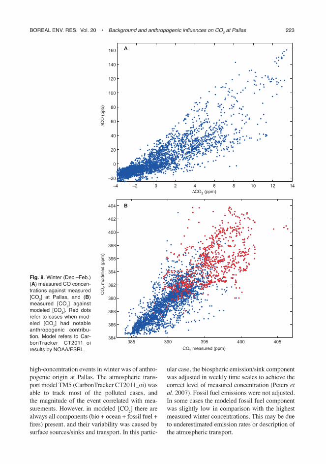
The absolute values of winter [CO] and [CO2] and modeled ff[CO2] were also studied. [CO2] and [CO] time series were pre-processed in a similar way by removing the species-dependent year-to-year growth trend and seasonal cycle. Winter [CO] and [CO2] measurements correlated (Pear-sons’s r = 0.87, p < 0.001) when focusing on the short term variability, i.e. a scale of anthropogenic pollution events (Fig. 8). CO2 concentrations measured in winter correlated with the modeled total [CO2] (Pearsons’s r = 0.85, p < 0.001). Cases when the modeled total [CO2] had highly elevated fossil fuel contribution (> 1 SD over background; cf. red dots in Fig. 8B). The modeled fossil fuel component correlated with measured [CO2] (Pear-sons’s r = 0.81, p < 0.001) and with [CO] (Pear-sons’s r = 0.77, p < 0.001).

Thus, according to the use of tracer for pol-luted air masses (CO), a large proportion of

365

370

375

380

385

390

395

400

405

410

100

125

150

175

200

225

250

275

CO

(ppb)

CO2 measuredCO2 total model (CT)CO2 anth model (CT)CO measured

CO

2 (p

pm)

Nov 2006 Jan 2007 Mar 2007 May 2007

Fig. 7. Pallas time series for measured CO2 con-centration, measured CO concentration, modeled co2 concentration and modeled anthropogenic contribution in [CO2]. note that the anthropogenic co2 concentrations have been moved up in scale for clarity. CT refers to CarbonTracker CT2011_oi results by NOAA/ESRL.


high-concentration events in winter was of anthro-pogenic origin at Pallas. The atmospheric trans-port model TM5 (CarbonTracker CT2011_oi) was able to track most of the polluted cases, and the magnitude of the event correlated with mea-surements. However, in modeled [CO2] there are always all components (bio + ocean + fossil fuel + fires) present, and their variability was caused by surface sources/sinks and transport. In this partic-

ular case, the biospheric emission/sink component was adjusted in weekly time scales to achieve the correct level of measured concentration (Peters et al. 2007). Fossil fuel emissions were not adjusted. In some cases the modeled fossil fuel component was slightly low in comparison with the highest measured winter concentrations. This may be due to underestimated emission rates or description of the atmospheric transport.

–4 –2 0 2 4 6 8 10 12 14–20

0

20

40

60

80

100

120

140

160

∆CO2 (ppm)

∆CO

(ppb

)

385 390 395 400 405384

386

388

390

392

394

396

398

400

402

404

CO2 measured (ppm)

CO

2 m

odel

led

(ppm

)

A

B

Fig. 8. Winter (Dec.–Feb.) (A) measured CO concen-trations against measured [CO2] at Pallas, and (B) measured [CO2] against modeled [CO2]. red dots refer to cases when mod-eled [CO2] had notable anthropogenic contribu-tion. Model refers to Car-bonTracker CT2011_oi results by NOAA/ESRL.


During summer, the anthropogenic contribu-tion in the measured [CO2] signal is masked by the strong biospheric component and enhanced photochemistry, and atmospheric mixing weak-ens the [CO] events. Thus we used model ff[CO2] in generalizing the results to cover the whole year. In tracking winter [CO2] measure-ments which were affected by relatively fresh anthropogenic emissions, all hours when [CO2] was elevated more than 1 SD over background were taken as polluted. The model fossil fuel component was used in a similar way for the whole year. For December–February, according to the measurements and model, the proportion of hours with notable anthropogenic influence was about 22%. For the whole year, according to the model, this proportion was about 10%. During the years 2006–2010, this proportion changed considerably with the greatest values occurring over the latest years (Table 1). The number of hours with a significant continental influence also increased when examining win-ters in different years, but not the whole years. In the light of the earlier results, we defined the significant continental contribution as “South” IR or “East” IR contributing > 40% to the total trajectory length.

The anthropogenic [CO2] almost always came from continental regions (as defined by

FLEXTRA influence regions). During winter, 86% of the model ff[CO2] hours had a signifi-cant continental contribution (Table 2). It has to be noted, however, that about 56%–63% of all significant “South” or “East” contributions were not anthropogenic, which means that all air flows from continental regions were not polluted and can thus be used in continental background studies. Only less than 9 hours out of about 500 elevated [CO2] or [CO] and model ff[CO2] hours were ‘mistakenly’ set as clean background according to FLEXTRA (Table 2), which con-firms the usefulness of the trajectory model in filtering MBL measurements. By looking at the whole year, the results were somewhat differ-ent: the number and intensity of anthropogenic events was smaller, and about 73%–80% of all substantial “South” or “East” contributions were not anthropogenic. The results for ele-vated [CO] and model ff[CO2] were similar to those in winter, but elevated [CO2] was not as strongly associated with air flows from “South” and “East” or CO/model results, indicating the presence of biogenic sources.

Summary and conclusions

Results from the two models, FLEXTRA and

Table 1. The fraction of hours (%) with elevated measured CO2 concentrations and model [CO2] anthropogenic component and substantial continental contribution (from FLEXTRA) in the Pallas data.

2006 2007 2008 2009 2010

Measured [CO2] winter 17 19 19 24 30Modelled ff[CO2] Winter 19 13 24 30 32 Whole year 9.1 8.7 11 13 11Continental Winter 48 32 44 46 66 Whole year 40 31 36 41 37

Table 2. The fraction of hours (%) with substantial continental or marine contribution (from FLEXTRA) in elevated measured CO2 and CO concentrations and in elevated model [CO2] anthropogenic component. Results from the years 2006–2009 were used.

High [CO2] High [CO2] High CO High CO Modeled ff[CO2] Modeled ff[CO2] winter total winter total winter total

continental 87 69 90 90 86 87marine 2.1 5.2 1.4 1.1 0 0.2


SILAM, were used in studying the influence regions (IR) on [CO2] measured at the Pallas station. FLEXTRA and SILAM produced similar synoptic-scale features regarding the air mass transport to Pallas, but there were also differ-ences that affected the classification of each measurement to a specific [CO2] IR. FLEX-TRA showed systematically higher contributions from “East” and “West” IR and SILAM from “South” and “Arctic” IR. SILAM also indicated stronger influence from “Local” IR. According to SILAM, high contributions (> 40%) from “Arctic” and “West” IR, i.e. marine IR, were often associated with low [CO2] measurements, while high “East” and “South” IR, i.e. conti-nental IR, contributions were connected with elevated [CO2]. FLEXTRA agreed with SILAM, though the results were more mixed.

The marine boundary layer signal was extracted from the measurements by using the model results and compared with the NOAA MBL reference. Both models performed well, with comparable annual amplitude and phase, and monthly deviations from the reference were usually inside 1 ppm. As compared with the mean seasonal cycle of the NOAA MBL refer-ence, SILAM did not have traces of elevated winter or lowered summer concentrations, while FLEXTRA had. However, the FLEXTRA MBL signal was only in a very few cases associated with measurements that were affected by anthro-pogenic emissions.

At Pallas, long-range-transported anthropo-genic emissions are observable in the concen-tration record especially during winter months. However, it has to be noted that due to these anthropogenic episodes the total atmospheric CO2 concentration at Pallas changes by only few percent (in absolute terms about 10–20 ppm). In practice, the effect of long-range-transported anthropogenic emissions on the CO2 concentra-tion at Pallas is thus very small. We used [CO] and the TM5 (CarbonTracker) model fossil fuel [CO2] component as a tracer for these emis-sions. The model captured the timing of high [CO2] as accurately as the anthropogenic tracer CO, both in over 70% of the high [CO2] hours during winter months. According to these trac-ers, the proportion of measurement hours with a noticeable anthropogenic influence in Decem-

ber–February at Pallas was over 20%, while for the whole year the proportion was about 10%. The anthropogenic proportion had largest values during the later years of the study period.

In conclusion, anthropogenic influences in the Pallas data can be tracked by the models and tracer measurements, and they can be asso-ciated with continental influence regions. The global background in [CO2] (MBL) is observ-able at Pallas, and it can be extracted by using information on marine influence regions. Both FLEXTRA and SILAM models performed well, but the SILAM results were more consistent and in a better agreement with the NOAA MBL reference. Therefore, moving from FLEXTRA to SILAM to estimate influence regions and a MBL signal at Pallas would be justified.

Acknowledgements: We would like to acknowledge Euro-pean Commission Life+ programme, SNOWCARBO proj-ect (LIFE07 ENV/FIN/000133), Finnish Academy Center of Excellence (project no. 111865) and ICOS 271878, ICOS-Finland 281255 and ICOS-ERIC 281250 funded by Academy of Finland. CarbonTracker CT2011_oi results were provided by NOAA ESRL, Boulder, Colorado, USA from the website at http://carbontracker.noaa.gov. We would like to acknowledge support from Nordic ministry of research (CarboNord project) and Academy of Finland (A4 project).

References

Aalto T., Hatakka J., Paatero J., Tuovinen J.-P., Aurela M., Laurila T., Holmen K., Trivett N. & Viisanen Y. 2002. Tropospheric carbon dioxide concentrations at a north-ern boreal site in Finland: basic variations and source areas. Tellus 54B: 110–126.

Biraud S., Ciais P., Ramonet M., Simmonds P., Kazan V., Monfray P., O’Doherty S., Spain G. & Jennings S.G. 2000. European greenhouse gas emissions estimated from continuous atmospheric measurements and radon 222 at Mace Head. J. Geophys. Res. 105: 1351–1366.

Bousquet P., Gaudry A., Ciais P., Kazan V., Monfray P., Simmonds P.G., Jennings S.G. & O’Connor T.C. 1996. Atmospheric CO2 concentration variations recorded at Mace Head, Ireland, from 1992 to 1994. Phys. Chem. Earth 21: 477–481.

Conway T.J., Tans P.P., Waterman L.S., Thoning K.W., Kitzis D.R., Masarie K.A. & Zhang N. 1994. Evidence for interannual variability of the carbon cycle from the NOAA/CMDL global air sampling network. J. Geophys. Res. 99: 22831–22855.

Eneroth K., Aalto T., Hatakka J., Holmén K., Laurila T. & Viisanen. Y. 2005. Atmospheric transport of carbon dioxide to a baseline monitoring station in northern Fin-land. Tellus 57B: 366–374.


Geels C., Gloor M., Ciais, P., Bousquet P., Peylin P., Vermeu-len, A.T., Dargaville R., Aalto T., Brandt J., Christensen J.H., Frohn L. M., Haszpra L., Karstens, U., Rödenbeck C., Ramonet M., Carboni G. & Santaguida R. Compar-ing atmospheric transport models for future regional inversions over Europe. 2007. Part 1: Mapping the CO2 atmospheric signals. Atmos. Chem. Phys. 7: 3461–3479.

GLOBALVIEW-CO2 2011. Cooperative Atmospheric Data Integration Project — Carbon Dioxide. CD-ROM, NOAA ESRL, Boulder, Colorado.

Granier C., Bessagnet B., Bond T., D’Angiola A., van der Gon H.D., Frost G.J., Heil A., Kaiser J.W., Kinne S., Klimont Z., Kloster S., Lamarque J.-F., Liousse C., Masui T., Meleux F., Mieville A., Ohara T., Raut J.-C., Riahi K., Schultz M.G., Smith S.J., Thomson A., van Aardenne J., van der Werf G.R. & van Vuuren D.P. 2011. Evolution of anthropogenic and biomass burning emissions of air pol-lutants at global and regional scales during the 1980–2010 period. Climatic Change 109: 163–190.

Hatakka J., Aalto T., Aaltonen V., Aurela M., Hakola H., Komppula M., Laurila T., Lihavainen H., Paatero J., Salminen K. & Viisanen Y. 2003. Overview of atmo-spheric research activities and results at Pallas GAW station. Boreal Env. Res. 8: 365–384.

Masarie K.A. & Tans P.P. 1995. Extension and integration of atmospheric carbon dioxide data into a globally consistent measurement record. J. Geophys. Res. 100: 11593–11610.

Olivier J.G.J, Van Aardenne J.A., Dentener F., Ganzeveld L. & Peters J.A.H.W. 2005. Recent trends in global green-house gas emissions: regional trends and spatial distribu-tion of key sources. Environ. Sci. 2: 81–99.

Peters W., Jacobson A.R., Sweeney C., Andrews A.E., Conway T.J., Masarie K., Miller J.B., Bruhwiler L.M.P., Petron G., Hirsch A.I., Worthy D.E.J., van der Werf G.R., Randerson J.T., Wennberg P.O., Krol M.C. & Tans P.P. 2007. An atmospheric perspective on North Amer-ican carbon dioxide exchange: CarbonTracker. Proc. Natl. Acad. Sci. USA 104: 18925–18930.

Peters W., Krol M.C., van der Werf G.R., Houweling S., Jones C.D., Hughes J., Schaefer K., Masarie K.A., Jacobson A.R., Miller J.B., Cho C.H, Ramonet M., Schmidt M., Ciattaglia L., Apadula F., Heltai D., Mein-hardt F., di Sarra A.G., Piacentino S., Sferlazzo D., Aalto T., Hatakka J., Ström J., Haszpra L., Meijer H.A.J., van der Laan S., Neubert R.E.M., Jordan A., Rodó X., Morgui J.-A., Vermeulen A.T., Rozanski K., Zimnoch

M., Manning A.C., Leuenberger M., Uglietti C., Dolman A.J., Ciais P., Heimann M. & Tans P.P. 2010. Seven years of recent European net terrestrial carbon diox-ide exchange constrained by atmospheric observations. Global Change Biology 16: 1317–1337.

Pommier M., McLinden C.A. & Deeter M. 2013. Relative changes in CO emissions over megacities based on observations from space. Geophys. Res. Let. 40, 3766, doi:10.1002/grl.50704.

Sofiev M., Siljamo P., Valkama I., Ilvonen M. & Kukkonen J. 2006. A dispersion modelling system SILAM and its evaluation against ETEX data. Atmos. Environ. 40: 674–685.

Sofiev M., Galperin M. & Genikhovich E. 2008. A construc-tion and evaluation of Eulerian dynamic core for the air quality and emergency modeling system SILAM. In: Borrego C. & Miranda A.I. (eds.) Air pollution model-ling and its application XIX, NATO Science for Peace and Security Series C: Environmental Security, Springer, pp. 699–701.

Stohl A., Wotawa G., Seibert P. & Kromp-Kolb H. 1995. Inter-polation errors in wind fields as a function of spatial and temporal resolution and their impact on different types of kinematic trajectories. J. Appl. Meteorol. 34: 2149–2165.

Stohl A. & Seibert P. 1998. Accuracy of trajectories as deter-mined from the conservation of meteorological tracers. Q. J. R. Meteor. Soc. 124: 1465–1484.

Thompson R., Manning A.C., Gloor E., Schultz U., Seifert T., Hänsel F., Jordan A. & Heimann M. 2009. In-situ measurements of oxygen, carbon monoxide and green-house gases from Ochsenkopf tall tower in Germany. Atmos. Meas. Tech. 2: 573–591.

Vermeulen A.T., Hensen A., Popa M. E., van den Bulk W.C.M. & Jongejan P.A.C. 2011. Greenhouse gas obser-vations from Cabauw Tall Tower (1992–2010). Atmos. Meas. Tech. 4: 617–644.

Vogel F.R., Hammer S., Steinhof A., Kromer B. & Levin I. 2010. Implication of weekly and diurnal 14C calibration on hourly estimates of CO-based fossil fuel CO2 at a moderately polluted site in southwestern Germany. Tellus 62B: 512–520.

Vogel F.R., Tiruchittampalam B., Theloke J., Kretschmer R., Gerbig C., Hammer S. & Levin I. 2013. Can we evaluate a fine-grained emission model using high-resolution atmospheric transport modelling and regional fossil fuel CO2 observations? Tellus 65B, 18681, doi:10.3402/tel-lusb.v65i0.18681.

background and anthropogenic influences on … and anthropogenic influences on atmospheric co 2...

Documents