bachelor thesis impact of random sweeping and turbulent ... · bachelor thesis impact of random...

Bachelor Thesis

Impact of Random Sweeping and Turbulent

Fluctuations on Lagrangian Transport in a

Model of Turbulence

Einfluss von ’Random Sweeping’ und turbulenten Fluktuationen aufLagrangeschen Transport in einem Turbulenz Modell

Student Tobias Wegener

[email protected]

Supervisor Dr. Michael Wilczek

[email protected]

Second Assessor Prof. Dr. Andreas Tilgner

[email protected]

Submission Date 08.04.2016

Contents

1 Introduction 1

2 Physical and Mathematical Background 6

2.1 Eulerian and Lagrangian View . . . . . . . . . . . . . . . . . . 62.2 Statistical Description of Turbulence . . . . . . . . . . . . . . 6

2.2.1 Averaging and Statistical Quantities . . . . . . . . . . . 72.2.2 Fourier Space Description . . . . . . . . . . . . . . . . 82.2.3 Energy Spectrum . . . . . . . . . . . . . . . . . . . . . 12

2.3 Stochastic Processes . . . . . . . . . . . . . . . . . . . . . . . 15

3 Turbulence as a Stochastic Process 17

3.1 Analytical Description . . . . . . . . . . . . . . . . . . . . . . 173.1.1 The Kraichnan Model as the Limit of a Finite-

Correlation-Time Model . . . . . . . . . . . . . . . . . 183.1.2 Random Sweeping . . . . . . . . . . . . . . . . . . . . 233.1.3 Summary . . . . . . . . . . . . . . . . . . . . . . . . . 25

3.2 Numerical Realisation . . . . . . . . . . . . . . . . . . . . . . 263.2.1 Generation of Correlated Velocity Fields . . . . . . . . 263.2.2 Integration Scheme . . . . . . . . . . . . . . . . . . . . 283.2.3 Implementation . . . . . . . . . . . . . . . . . . . . . . 283.2.4 Choice of the Parameters and Convergence . . . . . . . 29

4 Results 31

4.1 Single-Particle Dispersion . . . . . . . . . . . . . . . . . . . . 314.2 Two-Particle Dispersion . . . . . . . . . . . . . . . . . . . . . 344.3 Two-Time Two-Particle Dispersion . . . . . . . . . . . . . . . 37

5 Conclusion 40

5.1 Summary of the Results . . . . . . . . . . . . . . . . . . . . . 405.2 Evaluation of the Methods . . . . . . . . . . . . . . . . . . . . 44

A Eulerian Description of the Kraichnan Flow 46

B Energy Spectrum of Real Flows 50

C Validation of the Numerical Velocity Fields 54

Literature 57

I

List of Figures

2.1 Eulerian and Lagrangian Description . . . . . . . . . . . . . . 62.2 Turbulent Energy Cascade . . . . . . . . . . . . . . . . . . . . 122.3 Fourier Representation of Eddy Structures . . . . . . . . . . . 132.4 Random Walk and Wiener Process . . . . . . . . . . . . . . . 153.1 Finite-Correlation-Time Process . . . . . . . . . . . . . . . . . 183.2 Random Sweeping . . . . . . . . . . . . . . . . . . . . . . . . 233.3 Implementation of the Wave Vector Array . . . . . . . . . . . 284.1 Plot: Multi-Particle Dispersion . . . . . . . . . . . . . . . . . 314.2 Plot: Single-Particle Dispersion . . . . . . . . . . . . . . . . . 334.3 Plot: Two-Particle Dispersion . . . . . . . . . . . . . . . . . . 374.4 Cross Term in the Two-Time Dispersion . . . . . . . . . . . . 384.5 Plot:Two-Time Two-Particle Dispersion . . . . . . . . . . . . . 395.1 Dispersion Overview . . . . . . . . . . . . . . . . . . . . . . . 43B.1 Energy Spectrum of Real Flows . . . . . . . . . . . . . . . . . 51B.2 Variation of the Parameters in a 5/3 Energy Spectrum . . . . 53C.1 Sample Velocity Field . . . . . . . . . . . . . . . . . . . . . . . 54C.2 Gaussianity of the Numerical Velocity Fields . . . . . . . . . . 55C.3 Longitudinal and Transverse Correlation Function . . . . . . . 56

II

Nomenclature

Variables and Symbols

t time variablexi i-th component of the Eulerian coordinatesXi(t) i-th component of the Lagrangian coordinatesx, X, . . . vector variablesx, X, . . . absolute value of a vector variablevi(x, t) i-th component of the Eulerian (Kraichnan) velocity fieldDij one-time two-point velocity correlation tensorξij normalised two-point velocity correlation tensord dimension of space· Fourier transformed quantity· Fourier coefficientκ continuous wave vectork discrete wave vectorR,C,Z the real/complex/integer numbersLd cubic flow domain of edge length LL edge length of a cubic flow domain

Φij(κ) continuous spectral two-point correlation tensor

Φij(k) discrete spectral two-point correlation tensorE(κ) energy spectrumS(κ) geometric factor stemming from spherical integrationW (t) standard Wiener processτ correlation time∆t time incrementO(·) Landau symbolD0 diffusivity in the Kraichnan ensemblevrms root-mean-squared velocity of the Kraichnan ensembleui i-th component of the sweeping velocity fieldτsw sweeping correlation timeDsw sweeping diffusivity

Operators and Distributions

∂(·) partial derivative with respect to (·)〈 · 〉 ensemble average

III

F [·] Fourier transformF−1 [·] inverse Fourier transformδ·,· Kronecker deltaδ(·) Dirac delta distributionTr [·] trace of a tensorN (µ, σ2) Gaussian probability distributionU(ϕ1, ϕ2) Uniform probability distribution

Abbreviations

i. e. that is (id est)e. g. for example (exempli gratia)eq. equationfig. figurech. chapter1D, 2D, 3D one/two/three dimensionalIbid. same reference as the preceding one (ibidern)

IV

Acknowledgement

At this point I would like to thank everyone who supported me in the work

on my thesis.

I want to say a great thank you to my supervisor Dr. Michael Wilczek who

took a lot of his time for discussions with me and assisted me in an extent

which is – in my opinion – far beyond of what a student usually can expect.

I also appreciate the conversations about other related topics and his insights

into the working life of a researcher in the scientific community.

Furthermore I would like to express my thanks to Dr. Cristian Lalescu who

assisted me in numerical and mathematical issues and gave very helpful advice

regarding the writing of the thesis as well.

V

1 Introduction 1

1 Introduction

During my studies I have attended a couple of courses dealing with fluid

mechanics and its various applications. A recurring theme that appeared

in all of these courses was the role of turbulence, i. e. the characteristics of

highly irregular fluid motions.

The impact of turbulence is indeed very important in many different branches

of physics and engineering. For instance, the climate system is largely in-

fluenced by turbulent motions of the atmosphere and the oceans, and in

engineering a better understanding of turbulence helps to construct more

efficient aircraft and wind turbines to name but a few applications [Les97, ch.

1.2].

However, the fundamental properties of turbulence are not yet understood in

a satisfactory manner and therefore turbulence is still considered to be the

last remaining unsolved problem of classical mechanics [Dav04, ch. 1.7].

In this thesis a simplified toy model of turbulence is studied that was originally

suggested by the theoretical physicist Robert Kraichnan (1928-2008) in 1968.

This Kraichnan model describes the transport of (passive) tracer particles

in a stochastic flow and is completely analytically tractable. The intention

of this thesis is to analyse this transport both analytically and numerically.

In addition, the model will be extended by an additional random sweeping

term that generates a superimposed large-scale motion of the tracer particles.

Interesting questions will then be:

• What kind of Lagrangian motion is generated by this model?

• How is this behaviour affected by the superimposed random sweeping?

• What is the dependence on the time scales under consideration?

1 Introduction 2

Why Study Toy Models?

As with every physical problem, the most obvious approach to turbulence

would be to write down equations of motion, solve them and analyse the

properties of the solutions. The equations of motion for incompressible

Newtonian fluids (water and air can be regarded as such in most cases)

are given by the Navier–Stokes equations (derived from conservation of

momentum) and the continuity equation (the conservation of mass)

[

∂t + vj ∂xj− ν ∂xj

∂xj

]

vi = −∂xip

ρ+ fi (1.1)

∂xivi = 0 (1.2)

with ∂t and ∂xibeing the partial derivatives with respect to time/the spatial

coordinates, vi the velocity components, p the pressure, ρ the (constant) fluid

density and fi being external forces (e. g. gravity). However, the equations

(1.1)-(1.2) are in general extremely difficult to solve and analytical solutions

exist only for special cases. One of the most crucial obstacles is the non-

linearity vj ∂xjvi [Pop00, pp. 14,17] [CFG08, ch. 2.2.1].

Due to the rapid fluctuations and the random behaviour of turbulent flows

it seems to be a promising approach to proceed to equations of averaged,

statistical quantities rather than dealing with particular flow realisations.

Thereby one could focus on the universal features and maybe avoid some

of the mathematical difficulties. One can indeed write down an averaged

version of the Navier–Stokes equations. However, a new problem arises as

there appear other averaged terms that are so far undetermined and must

somehow be related back to the flow to obtain a closed system of equations. A

universal, satisfying closure is not yet known though [Dav04, ch. 1.7][DPR03,

ch. 1][Pop00, ch. 4.2].

Yet another different approach was published in 1941 by Andrej Kolmogorov

which is now referred to as the K41 (Kolmogorov 1941) theory. He derived

some specific laws for turbulent flows just by dimensional analysis based on

1 Introduction 3

a few reasonable hypotheses. The predictions of this theory turned out to

be in quite good agreement with experimental results but covered only some

aspects of turbulence theory [DPR03, ch. 2.1][Les97, ch. 6.4].

Until now there is no comprehensive, universal statistical description of

turbulence that is derived from first principles and capable of explaining

what is observed in experiments. Therefore the most common strategy in

turbulence theory has become to tackle turbulence from different perspectives

by focussing on individual aspects and their causes and thereby develop a

more thorough general understanding of turbulence [Dav04, p. 102].

The Kraichnan model which was mentioned before can be regarded as one such

contribution. Its outstanding advantage is that it is completely analytically

tractable.

The Kraichnan Model

The underlying idea was to consider a purely kinematic model of turbulence

where the velocity fields are prescribed (with well-defined statistics) and in

which one analyses the dispersion of a passive scalar (i. e. fields or tracer

particles that are carried around by the flow without any backwards influence).

The velocity fields are taken to be Gaussian (i. e. the velocities are normally

distributed) and completely decorrelated in time (i. e. the field is supposed

to be varying extremely rapidly) in order to make the problem analytically

tractable.

The last two properties are rather far from being realistic because real flows

exhibit neither Gaussian velocity statistics nor an infinitely-rapid decorrelation

in time, but these properties ultimately facilitate an analytical treatment

[Ber00, ch. 3.2].

Under these assumptions the velocity statistics are completely defined by the

mean (which is chosen to be vanishing for convenience) and the two-time

1 Introduction 4

two-point correlation tensor [CFG08, ch. 2.4]

〈 vi(x, t) 〉 = 0 (1.3)

〈 vi(x, t) vj(x + r, t′) 〉 = Dij(x, r) δ(t − t′) (1.4)

where Dij characterises the simultaneous spatial correlation. The delta

function gives rise to infinitely-rapid decorrelation in time and ensures that

time integrals can be solved easily. More information about these quantities

follows in chapter 2.2.1.

Even though the Kraichnan model is formally well-defined, there are some

peculiarities involved whose interpretation is not trivial at first glance:

• According to the very definition, the velocities in the Kraichnan model

are actually infinite because of the delta function. But what is the

physical meaning of such infinite velocities? How are these interpreted

when appearing in integrals?

• Furthermore, how can these be implemented numerically? A computer

is not capable of dealing with infinite quantities and consequently a

workaround is required.

There are a couple of publications dealing with the Kraichnan model (e. g.

[CFG08, Ber00, FGV01]) but these make use of mathematical tools (stochas-

tic calculus and field-theoretical approaches such as renormalisation group

methods, path integral formulations, operator product expansions, . . . ) which

are beyond the standard mathematical education of physics students. These

publications are hence only of limited help for an initial understanding if a

background in these tools is missing.

A central part of this thesis will therefore be chapter 3.1 in which the Kraichnan

model is derived heuristically as the limit of a finite-correlation time process.

Simultaneously the aforementioned issues will be resolved such that actual

calculations and simulations can be performed.

1 Introduction 5

Overview of the Thesis

This thesis is structured as follows:

Initially (ch. 2) a physical and mathematical background is given as an

overview over the methods and the terminology used later on. It deals with

the statistical description of turbulence (both in real and Fourier space) as

well as stochastic processes.

The main part of the thesis is composed of two aspects: In chapter 3 there

is a heuristic derivation of how turbulence can be modelled as a stochastic

process (in accordance with Kraichnan’s description) both analytically (ch.

3.1) and numerically (ch. 3.2). In that context the random sweeping extension

of the Kraichnan model will also be introduced (ch. 3.1.2). The second main

aspect (ch. 4) is the actual analysis of the Lagrangian transport within the

Kraichnan model and supplemented sweeping.

The actual thesis is completed by a discussion section which summarises the

results and discusses the methods that were used (ch. 5).

Lastly there is also an appendix in which related topics are covered which

are not crucial for the understanding of the thesis but might be interesting as

well in this context.


2 Physical and Mathematical Background

2.1 Eulerian and Lagrangian View

For the description of the time evolution of a fluid flow one can use either the

Eulerian or the Lagrangian view.

Eulerian Lagrangian

Figure 2.1: Difference of the Eulerian (description in terms of fixed points inspace/fields) and the Lagrangian (motion of fluid elements along trajectories)picture.

In the Eulerian view one analyses the time evolution of the field vi(x, t) at

fixed points x in space. On the contrary, in the Lagrangian view one looks

at individual tracer particles/small volume elements that are transported by

the flow. At some initial time t0 a trajectory X(t) is assigned to a point x0 in

space such that X(t0) = x0. Then X(t) gives the position of that particle for

all later times t. The evolution of the deterministic Lagrangian trajectories is

then given by [Pop00, ch. 2.2]:

dXi(t) = vi(X(t), t) dt (2.1)

2.2 Statistical Description of Turbulence

The complexity and the chaotic behaviour of turbulent flows calls for a de-

scription in terms of statistical quantities. In the following, suitable statistical

quantities are introduced and put into the context of turbulent flows.


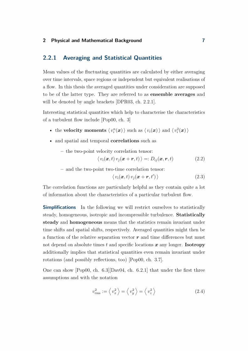
2.2.1 Averaging and Statistical Quantities

Mean values of the fluctuating quantities are calculated by either averaging

over time intervals, space regions or independent but equivalent realisations of

a flow. In this thesis the averaged quantities under consideration are supposed

to be of the latter type. They are referred to as ensemble averages and

will be denoted by angle brackets [DPR03, ch. 2.2.1].

Interesting statistical quantities which help to characterise the characteristics

of a turbulent flow include [Pop00, ch. 3]

• the velocity moments 〈 vni (x) 〉 such as 〈 vi(x) 〉 and 〈 v2

i (x) 〉

• and spatial and temporal correlations such as

– the two-point velocity correlation tensor:

〈 vi(x, t) vj(x + r, t) 〉 =: Dij(x, r, t) (2.2)

– and the two-point two-time correlation tensor:

〈 vi(x, t) vj(x + r, t′) 〉 (2.3)

The correlation functions are particularly helpful as they contain quite a lot

of information about the characteristics of a particular turbulent flow.

Simplifications In the following we will restrict ourselves to statistically

steady, homogeneous, isotropic and incompressible turbulence. Statistically

steady and homogeneous means that the statistics remain invariant under

time shifts and spatial shifts, respectively. Averaged quantities might then be

a function of the relative separation vector r and time differences but must

not depend on absolute times t and specific locations x any longer. Isotropy

additionally implies that statistical quantities even remain invariant under

rotations (and possibly reflections, too) [Pop00, ch. 3.7].

One can show [Pop00, ch. 6.3][Dav04, ch. 6.2.1] that under the first three

assumptions and with the notation

v2rms :=

⟨

v2x

⟩

=⟨

v2y

⟩

=⟨

v2z

⟩

(2.4)


the two-point velocity correlation tensor can be written as:

Dij(r) = v2rms

[

g(r) δij + [f(r) − g(r)]rirj

r2

]

︸︷︷︸

:=ξij(r)

(2.5)

Here ξij is the correlation tensor normalised by v2rms = Dij(0) such that

ξij(0) = 1 and ≤ 1 otherwise. Because of isotropy, ξij can only be composed

of isotropic tensors. It turns out that the only isotropic second-rank tensors

(which might be functions of a vector r) are the Kronecker delta δij and the

product of the two respective components, namely rirj. The factors in front of

these tensors must then only depend on the absolute value of r [Ibid.].

The motivation behind expressing these factors in terms of a function f and

g is the following: If r!

= r ex, then one finds that f and g represent the

longitudinal and transverse correlation functions respectively [Ibid.]:

ξxx(rex) = f(r) ξyy(rex) = ξzz(rex) = g(r) (2.6)

Incompressible velocity fields additionally fulfil the continuity restriction

∂xiDij = 0. This links the functions f and g to each other by the condi-

tion

g(r) = f(r) +r

2∂rf(r) (2.7)

in the 3D case (and without the factor 2 in the 2D case) [Ibid].

2.2.2 Fourier Space Description

The following calculations are guided by similar ones in [Pop00, ch. 6] and

[DPR03, ch. 9].

Fourier Transform A d-dimensional velocity field can be described both in

real space and in Fourier space. The different fields are related by the Fourier


transform F [·] and its inverse F−1 [·] defined as follows [DPR03, ch. 9]:

vi(κ) := F [vi(x)] (κ) :=1

(2π)d

∫

Rdvi(x) e−iκ·x dd

x (2.8)

vi(x) := F−1 [vi(κ)] (x) :=∫

Rdvi(κ) eiκ·x dd

κ, vi(κ) ∈ C (2.9)

These transforms can even be applied to spatially unbounded fields vi(x).

The Fourier transformed velocity field vi(κ) is a complex field but it has to

exhibit Hermitian symmetry in order to produce a real-valued velocity field

vi [Pop00, app. E]:

vi(κ) = v∗i (−κ) (reality condition) (2.10)

Fourier Series In the special case of a spatially bounded flow in a cubic box

with periodic boundary conditions the velocity field can even be expanded

as a Fourier series, i. e. a discrete superposition of infinitely many complex

Fourier modes vi(k) eik·x. Let the edge length of the box be labelled L and

the set of points within the box be denoted by Ld. Then the real velocity

field vi(x) and the complex Fourier coefficients vi(k) are related as follows

[Pop00, ch. 6.4.1]:

vi(x) =∑

k

vi(k) eik·xk ∈

{

n2π

L

∣∣∣∣ n ∈ Z

d}

(2.11)

vi(k) =1

Ld

∫

Ldvi(x) e−ik·x dd

x ∈ C (2.12)

Note that the continuous wave vectors were denoted by κ while now a k is

used for the discrete ones. Likewise, the continuous Fourier transforms are

labelled by a tilde whereas a hat is used for the discrete Fourier modes.

Equation (2.12) can easily be verified by linking the values of the discrete

Fourier coefficients to the continuous Fourier transforms (on the same cubic

domain Ld):


vi(k)(2.8)=

1

(2π)d

∫

Ldvi(x) e−ik·x dd

x(2.11)=

1

(2π)d

∑

k′

vi(k′)∫

Ldei(k′−k)·x dd

x

=1

(2π)d

∑

k′

vi(k′) Ld δk,k′ =

(L

2π

)d

vi(k) (2.13)

Here δk,k′ is a generalised version of the Kronecker delta. It results from the

orthonormality of the complex exponentials: For k′ − k 6= 0 the integral

vanishes due to the periodicity of the integrand. Otherwise the integrand

becomes unity and the integral is equal to the domain volume Ld.

Velocity Correlations In real space the (homogeneous) two-point velocity

correlation tensor was given by eqs. (2.2) and (2.5):

〈 vi(x) vj(x + r) 〉 = Dij(r) = v2rms ξij(r) (2.14)

For statistical calculations in Fourier space it is necessary to have an expression

for the spectral velocity correlation functions as well. In the case of continuous

wave vectors it reads (using a substitution x′ = x + r):

〈 vi(κ) vj(κ′) 〉 (2.8)

=1

(2π)2d

∫

Rd

∫

Rd〈 vi(x) vj(x + r) 〉 e−i(κ+κ′)·x e−iκ′·r dd

x ddr

(2.14)=

1

(2π)2d

∫

RdDij(r) e−iκ′·r dd

r

∫

Rde−i(κ+κ′)·x dd

x

︸︷︷︸

(2π)d δ(κ+κ′)

(2.8)=

1

(2π)d

∫

RdDij(r) e−iκ′·r dd

r

︸︷︷︸

=F [Dij(r)]

δ(κ + κ′) (2.15)

Here δ(κ + κ′) denotes the Dirac delta distribution. Apparently, the Fourier

coefficients are uncorrelated unless κ′ = −κ. The reason is that the real space

correlation tensor is independent of x due to homogeneity and can therefore

be written outside the x integral.


Analogously, for the discrete case one finds:

〈 vi(k) vj(k′) 〉 (2.12)

=1

L2d

∫

Ld

∫

Ld〈 vi(x) vj(x + r) 〉 e−i(k+k

′)·x e−ik′·r ddx dd

r

=1

Ld

∫

LdDij(r) e−ik′·r dd

r δk,−k′ (2.16)

(2.12)= Dij(k

′) δk,−k′ (2.17)

⇔ Dij(r) =∑

k

Dij(k) eik·r with Dij(k) = 〈 vi(k) vj(−k) 〉 (2.18)

which restates the previous result (that Fourier coefficients with k′ 6= −k are

uncorrelated) for the periodic case.

Spectral Correlation Tensor The quantity

Φij(κ) := F [Dij](κ) =1

(2π)d

∫

RdDij(r) e−iκ·r dd

r (2.19)

which appears in eq. (2.15) is referred to as the spectral correlation ten-

sor and it completely specifies two-point correlations in homogeneous turbu-

lence.

If the flow under considerations is even isotropic and incompressible (see ch.

2.2), then it can be shown (see [Pop00, ch. 6.5.1]) that the most general shape

of Φij is

Φij(κ) = A(κ) δij + B(κ)κiκj

κ2(+ isotropy) (2.20)

Φij(κ) = C(κ)(

δij − κiκj

κ2

)

(+ continuity) (2.21)

with A, B and C being so far undetermined functions.

Analogously to eq. (2.13), its discrete equivalent reads:

Φij(k) =(

2π

L

)d

Φij(k) (2.22)


2.2.3 Energy Spectrum

Figure 2.2: De-cay of eddiesduring the en-ergy cascade.

Energy Cascade In a turbulent flow one qualitatively

observes the following behaviour: In the transition from a

laminar to a turbulent flow the large-scale motion becomes

unstable and eddy-like structures evolve with a size com-

parable to the dimension of the system. These large-scale

eddies might still be influenced significantly by the geome-

try of the system. However, due to non-linear effects these

eddy structures are not stable either and decay into smaller

and smaller ones. Thereby the kinetic energy of the flow is

passed on to more and more confined scales (see fig. 2.2).

This way of looking at turbulence was first mentioned by

Richardson in the 1920’s [Dav04, ch. 1.6][Ric07].

Role of Different Scales The flow behaviour on the largest scales is strongly

affected by the specific set-up (defined by the boundary conditions as well

as the forcing, i. e. the way energy is supplied to the system) whereas on

sufficiently small scales the local flow is not even turbulent any longer. Here

viscous effects become relevant (due to a larger shear stress) and suppress

the turbulent fluctuations [Dav04, ch. 1.6].

If one is interested in universal properties of turbulence one must therefore

focus on intermediate length scales in between these extremes. The corre-

sponding range of universal turbulent scales is referred to as inertial range.

[Dav04, ch 3.2.6]

Definition of the Energy Spectrum The energy that is stored within a

specific spatial scale can easily be analysed in Fourier space. As can be seen in

figure 2.3, a wave vector κ with a corresponding wavelength λ = 2π/κ [Pop00,

ch. 6.4.1] can be associated with eddy structures of diameter d = λ/2 = π/κ.

Hence the Fourier coefficients vi(κ) with |κ| ≈ κ provide a measure of how

much kinetic energy is stored in the eddies of size d ≈ π/κ.

This qualitative idea can be quantified by means of the spectral correlation


velocity profile

eddy structure

Figure 2.3: Fourier modes of wavelength λ can be associated with eddies ofdiameter d ≈ λ/2.

tensor (eq. 2.21) [Pop00, ch. 3.7]: What is the amount of energy E stored in

an infinitesimal band of wavelengths [κ, κ + dκ] ?

E(κ) =∫

Rd

〈 v(κ) · v(κ)∗ 〉2

δ(|κ| − κ) ddκ (2.23)

2.21=∫

Rd

Tr[Φij](κ)

2δ(|κ| − κ) dd

κ (2.24)

=Tr[Φij](κ)

2S(κ) (2.25)

with

S(κ) =

2πκ d = 2

4πκ2 d = 3(2.26)

being a geometric factor stemming from the spherical integration (which

depends on the dimension d).

The function E(κ) is called the energy spectrum. In the case of incom-

pressible and isotropic turbulence the knowledge of this function suffices to

determine the spectral correlation tensor (2.21) [Pop00, ch. 6.5.1][DPR03, ch.

9.2]:

Φij(κ) = C(κ)[

δij − κiκj

κ2

]

with C(κ) =2E(κ)

(d − 1)S(κ)(2.27)

Here it was used that Tr[Φij](κ) = (d − 1) C(κ).


According to (2.22) the discrete equivalent of this tensor for the 2D case then

reads:

Φij(k)(2.22)=

4πE(κ)

kL2

[

δij − kikj

k2

]

(2.28)

This expression will be used later on for the numerical generation of the

correlated random velocity fields (see ch. 3.2).


2.3 Stochastic Processes

Stochastic processes are defined in terms of probabilistic predictions rather

than deterministic ones.

A simple example of a stochastic process is the one-dimensional random walk

(see fig. 2.4). It is a time-discrete process that describes the stochastic 1D

motion of a particle that is subject to probabilistic displacements (drawn from

a normal distribution) between these discrete times [Ste13, ch. 1.7].

Wiener Process In the scaling limit of infinitesimally small time increments

the stochastic kicks are no longer discrete in time and the random walk

converges to a so-called Wiener process W (t) (see fig. 2.4).

0 1 2 3 4 5 6

t

−40−30−20−10

010203040

X(t)

Random Walk

0 1 2 3 4 5 6

t

Wiener Process

Figure 2.4: A Wiener process can be looked at as a random walk withinfinitesimally small time steps. In that limit the curve has a self-similarshape, i. e. any arbitrarily small segment looks similar to the macroscopicjagged shape. It remains continuous in time but is no longer differentiableanywhere.

A standard Wiener process is formally defined by the following properties

[Fuc13, ch. 3.1.1]:

• W (t0) = 0

• W (t) is almost surely continuous in time

• W (t) has stationary, independent increments W (t + ∆t) − W (t)


• the increments are normally distributed with distribution ∼ N (0, ∆t)

These definitions have a couple of implications: For a given value W (t) the

best guess for any future value W (t + ∆t) is the current one because the

expectation value of the increments is zero. The mean-squared displacement

(hence the variance of the increments) during a time step ∆t is given by⟨

(W (t + ∆t) − W (t))2⟩

= ∆t such that the root-mean-squared displacement

goes as ∼√

∆t. Furthermore, even though the Wiener process is almost

surely continuous in time, it is nowhere differentiable [Fuc13, ch. 3.1.1][Ste13,

ch. 2.10].

An important physical example that is modelled as a Wiener process is

Brownian motion Here the motion of a rather large particle originates

from collisions with smaller, more rapidly moving particles. The macroscopic

motion appears to be completely random and can be approximated by a

Wiener process [Fuc13, ch. 3.1].

Langevin Equation An equation of motion for a particle in a stochastic

process is given by the so-called Langevin equation. It can be regarded

as the stochastic counterpart to the Lagrangian equation of motion of a

deterministic process (2.1) and can be given both in differential and integral

form. A particular Langevin equation might look like this:

dX(t) = v(X(t), t) dt + b(X(t), t) dW (differential) (2.29)

X(t + ∆t) =∫ t+∆t

tv(X(t′), t′) dt′ +

∫ ∆t

tb(X(t′), t′) dW (t′) (integral)

(2.30)

Here v and b are arbitrary functions that might depend on both time t and

the stochastic process X(t).

The integral representation contains an ordinary integral with respect to t

and a stochastic one which requires a special treatment. There are different

but equivalent interpretations of such stochastic integrals, e. g. the Ito- and

the Stratonovich one. More on this can be read e. g. in [Maz02, ch. 3.7][Ste13,

ch. 2][Fuc13, ch. 3.1.3][Bir13, ch. 1.6.2].


3 Turbulence as a Stochastic Process

3.1 Analytical Description

The chaotic and random behaviour of turbulent flows suggests to describe

turbulence as a stochastic process. One is tempted to proceed in a similar

fashion as in the case of Brownian motion which is modelled as a Wiener

process. There arise however a few obstacles:

• From a physical perspective turbulence is described in terms of velocity

statistics such as the energy spectrum or the corresponding velocity

correlation tensor. Stochastic processes like the Wiener process are

however nowhere differentiable and therefore velocities are not defined

in the conventional sense (i. e. v = x). How is it possible to construct a

stochastic processes that obeys certain velocity statistics?

• Furthermore, in the Brownian motion case the particles move inde-

pendently of each other whereas in turbulent motion there is a spatial

correlation. In that case adjacent particles move alongside each other

when being sufficiently close to each other. How can this correlation be

included in the modelling?

In the following I will heuristically derive a stochastic process that both

generates stochastic trajectories and simultaneously allows for a calculation of

velocity statistics. This is achieved by introducing a finite correlation time τ

(similar to the random walk case). A delta-correlated stochastic process will

then be obtained in the limit of infinitesimally small correlation time (accom-

panied by a proper rescaling of the velocity field). This approach eventually

reproduces the idea presented in Kraichnan’s 1968 paper [Kra68].


3.1.1 The Kraichnan Model as the Limit of a Finite-

Correlation-Time Model

The key idea is to make use of random but correlated Eulerian velocity

fields vi(x, t) (see fig. 3.1). These are assumed to be constant over some

time interval τ before being instantly replaced by a new one. The particle

trajectories Xi(t) are then continuous in time but the stochastic changes occur

only at discrete times ta separated by the correlation time τ (see fig. 3.1). At

each time ta a new velocity field is generated and persists until the next time

step ta+1 = ta + τ .

t0 t1 t2 t3 t4 t5 t6 t

τ

. . .

v(x, t0) v(x, t1) v(x, t2)

Xi(t)

Figure 3.1: Sketch of the time-continuous process in which stochastic effectsonly occur at discrete times ta. There the velocity fields are instantly replacedby independent new ones.

Within these time intervals the particle motion is to first order ballistic:

Xi(ta+1) = Xi(ta) +∫ ta+1

ta

vi(X(t), t) dt = Xi(ta) +∫ ta+1

ta

vi(X(ta), ta) + O(t) dt

= Xi(ta) + vi(X(ta), ta) τ + O(τ 2) (3.1)

Two-Time Correlation The simultaneous velocity statistics are then given

by the mean and some two-point correlation tensor (see ch. 2.2):

〈 vi(x, t) 〉 = 0 for convenience (3.2)

〈 vi(x) vj(x + r) 〉 = v2rms ξij(r) two-point correlation tensor (3.3)


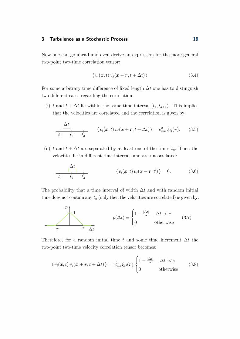
Now one can go ahead and even derive an expression for the more general

two-point two-time correlation tensor:

〈 vi(x, t) vj(x + r, t + ∆t) 〉 (3.4)

For some arbitrary time difference of fixed length ∆t one has to distinguish

two different cases regarding the correlation:

(i) t and t + ∆t lie within the same time interval [ta, ta+1). This implies

that the velocities are correlated and the correlation is given by:

t1 t2 t3

∆t〈 vi(x, t) vj(x + r, t + ∆t) 〉 = v2

rms ξij(r). (3.5)

(ii) t and t + ∆t are separated by at least one of the times ta. Then the

velocities lie in different time intervals and are uncorrelated:

t1 t2 t3

∆t〈 vi(x, t) vj(x + r, t′) 〉 = 0. (3.6)

The probability that a time interval of width ∆t and with random initial

time does not contain any ta (only then the velocities are correlated) is given by:

p

∆tτ−τ

1p(∆t) =

1 − |∆t|τ

|∆t| < τ

0 otherwise(3.7)

Therefore, for a random initial time t and some time increment ∆t the

two-point two-time velocity correlation tensor becomes:

〈 vi(x, t) vj(x + r, t + ∆t) 〉 = v2rms ξij(r)

1 − |∆t|τ

|∆t| < τ

0 otherwise(3.8)


Long Time Behaviour Now general time increments ∆t will be considered

which satisfy ∆t ≫ τ . On these time scales the process appears to be purely

stochastic (like the Wiener process). For technical reasons it will be assumed

that ∆t is an integer multiple of τ . One of the major capabilities of the finite-

correlation-time model is that Lagrangian increments can still be related to

actual physical velocities via the correlation time τ :

Xi(t + ∆t)(3.1)= Xi(t) +

∆tτ

−1∑

a=0

[

vi(X(t + aτ), t + aτ) τ + O(τ 2)]

(3.9)

Averaged quantities can be specified even further (summation not implied):

〈 Xi(t + ∆t) − Xi(t) 〉 =

⟨ ∆tτ

−1∑

a=0

vi(X(t + aτ), t + aτ) τ

⟩

+ O(τ)

=

∆tτ

−1∑

a=0

〈 vi(X(t + aτ), t + aτ) 〉︸︷︷︸

(3.2)= 0

τ + O(τ)

= O(τ) (3.10)

⟨

[Xi(t + ∆t) − Xi(t)]2⟩

=

⟨ ∆tτ

−1∑

a=0


∆tτ

−1∑

b=0

vi(X(t + bτ), t + bτ) τ

⟩

+ O(τ 2)

=

∆tτ

−1∑

a=0

∆tτ

−1∑

b=0

〈 vi(X(t + aτ), t + aτ) vi(X(t + bτ), t + bτ) 〉 τ 2 + O(τ 2)

(3.8)=

∆tτ

−1∑

a=0

⟨

vi(X(t + aτ), t + aτ)2⟩

τ 2 + O(τ 2)

= v2rms τ 2 ∆t

τ+ O(τ 2) = v2

rmsτ ∆t + O(τ 2) (3.11)


Here the fact was used that – within this model – velocities are uncorrelated

for time differences greater than or equal to τ . Hence, in the sum all but the

simultaneous terms vanish and the double sum reduces to a single one.

An important insight from this calculation is that over time increments

∆t ≫ τ the displacement statistics of particles do (to second order) only

depend on a single quantity D0 := v2rmsτ (called diffusivity) [FGV01, ch. II]

which defines the pace of displacement in a stochastic process.

Transition to a Delta-Correlated Process The transition from this finite-

correlation-time model to a delta-correlated stochastic process is now obvious:

One takes the limit τ → 0 in such a fashion that the long-time behaviour is

unaffected (D0 remains constant, v2rms rescales to infinity).

Together with eqs. (3.3) and (3.8) (and inserting a factor ττ

= 1) this implies

for the general two-point two-time correlation function:

〈 vi(x, t) vj(x + r, t + ∆t) 〉 = limτ→0

τ v2rms

︸︷︷︸

=D0

ξij(r)1

τ

1 − |∆t|τ

|∆t| < τ

0 otherwise

= D0 ξij(r) limτ→0

1

τ

1 − |∆t|τ

|∆t| < τ

0 otherwise

= D0 ξij(r) δ(∆t) (3.12)

Hence, the velocity field becomes a so-called delta-correlated Gaussian white

noise [Fuc13, ch. 3.1.3] with respect to time and its spatial correlation is now

given by D0 ξij(r). Equivalently, eq. (3.9) turns into the integral form of the

Langevin equation of the process:

Xi(t + ∆t) = Xi(t) + limτ→0

∆tτ

−1∑

a=0


= Xi(t) +∫ t+∆t

tvi(X(t′), t′) dt′ (3.13)


The integrals which involve delta-correlated (and hence infinite) velocities are

properly defined if the quantities under consideration are eventually averaged

such that the conditions (3.12) and 〈 vi 〉 = 0 can be applied.

Numerical Integration Scheme A sample trajectory with the statistical

properties (3.10) and (3.11) is given by the following increments:

Xi(t + ∆t) = Xi(t) + vi(X(t), t)√

τ√

∆t

Here vi(x, t) is a Gaussian random field. In the rescaling limit τ is actually

zero and vi becomes infinite. This cannot be treated numerically but the

problem is avoided by using the finite diffusivity D0 = v2rmsτ instead:

Xi(t + ∆t) = Xi(t) + vi(X(t), t)

√

D0

v2rms

√∆t

= Xi(t) +√

D0vi(X(t), t)

vrms

√∆t

= Xi(t) +√

D0 ∆Wi(X(t), t)

Here vi(X(t),t)vrms

is a Gaussian random field normalised by its standard deviation.

When multiplied by√

∆t, this becomes a standard Wiener process Wi(X(t), t).

The descriptions is then analogous to the Brownian motion case except for

that the velocities and hence the Wiener increments are spatially correlated

over coinciding time intervals

〈 ∆Wi(X(t), t) ∆Wj(X′(t), t) 〉 (3.13)(3.12)

= D0

∫ t+∆t

tξij (X ′(s) − X(s)) ds

(3.14)

and zero for non-overlapping time intervals (due to the independence of the

increments of the Wiener process).


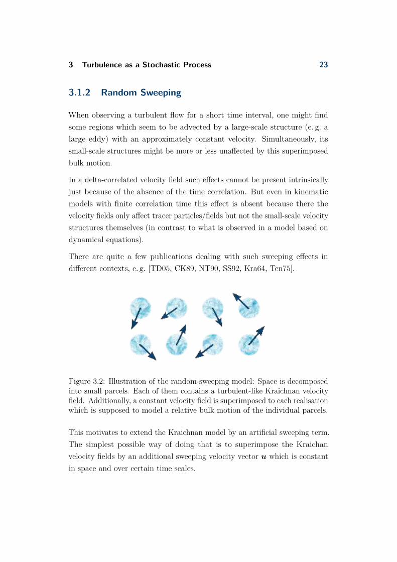
3.1.2 Random Sweeping

When observing a turbulent flow for a short time interval, one might find

some regions which seem to be advected by a large-scale structure (e. g. a

large eddy) with an approximately constant velocity. Simultaneously, its

small-scale structures might be more or less unaffected by this superimposed

bulk motion.

In a delta-correlated velocity field such effects cannot be present intrinsically

just because of the absence of the time correlation. But even in kinematic

models with finite correlation time this effect is absent because there the

velocity fields only affect tracer particles/fields but not the small-scale velocity

structures themselves (in contrast to what is observed in a model based on

dynamical equations).

There are quite a few publications dealing with such sweeping effects in

different contexts, e. g. [TD05, CK89, NT90, SS92, Kra64, Ten75].

Figure 3.2: Illustration of the random-sweeping model: Space is decomposedinto small parcels. Each of them contains a turbulent-like Kraichnan velocityfield. Additionally, a constant velocity field is superimposed to each realisationwhich is supposed to model a relative bulk motion of the individual parcels.

This motivates to extend the Kraichnan model by an artificial sweeping term.

The simplest possible way of doing that is to superimpose the Kraichan

velocity fields by an additional sweeping velocity vector u which is constant

in space and over certain time scales.


In particular, the sweeping velocities will be drawn from a normal distribution

ui ∼ N (0, u2rms) and are assumed to have some (rather large) correlation

time τsw under which they are constant before being replaced by a new

velocity immediately. This is a slight extension of the most simple sweeping

(completely constant in time). It ensures that the sweeping still gives rise

to a diffusive long-term behaviour as being typical for turbulence [MY75, ch.

9.3].

The sweeping statistics are hence defined by:

〈 ui 〉 =

ui on time scales ≪ τsw

0 on time scales ≫ τsw

(3.15)

〈 ui(x, t) uj(x + r, t + ∆t) 〉 (3.8)= urms

1 − ∆tτsw

∆t < τsw

0 otherwise(3.16)

As with the Kraichnan fields, the latter can be interpreted as:

〈 ui(x, t) uj(x + r, t + ∆t) 〉 (3.8)=

ui uj on time scales ≪ τsw

u2rms τsw︸︷︷︸

:=Dsw

δ(∆t) on time scales ≫ τsw

(3.17)

In the calculations two different kinds of averages will be used. The first one

〈 · 〉 implies averaging over blobs with the same sweeping velocity whereas

the second one 〈 · 〉sw additionally averages over the ensemble of sweeping

velocities (and hence all the different blobs as in fig. 3.2.


3.1.3 Summary

The Lagrangian trajectories in a flow that is composed of a Kraichnan velocity

field and an additional sweeping term are defined in terms of stochastic integral

equations:

Xi(t2) = Xi(t1) +∫ t2

t1

ui(t) dt︸︷︷︸

sweeping

+∫ t2

t1

vi(X(t), t) dt︸︷︷︸

Kraichnan

(3.18)

The integrals which involve delta-correlated (and hence infinite) velocities

vi can be evaluated properly if the quantities under consideration are even-

tually averaged. Then one can use that vi is Gaussian with the following

properties:

〈 vi 〉 = 0

〈 vi(x, t) vi(x + r, t′) 〉 = D0 ξij(r) δ(t − t′)

(3.19)

(3.20)

and evaluate the remaining integrals using the rules of classical calculus. The

sweeping fields ui are treated likewise on time scales large compared to the

sweeping correlation time τsw (see eq. (3.17)) and assumed to be constant on

time scales ≪ τsw.

A numerical integration scheme of this process is given by:

Xi(t + ∆t) = Xi(t) + ui ∆t +√

D0vi(X(t), t)

vrms

√∆t (3.21)


3.2 Numerical Realisation

In addition to the analytical calculations the Kraichnan model will be analysed

numerically as well. The procedure is to create a new random velocity field at

each time step and to integrate Lagrangian trajectories by means of a proper

integration scheme that reproduces the analytical description.

For the implementation the programming language python has been used.

The core is the generation of Kraichnan velocity fields in Fourier space (where

the correlation restrictions can be implemented easily) and their conversion

to real velocities by means of a discrete Fourier transform. For the latter the

pyFFTW package has been used which provides an interface to the FFTW (Fastest

Fourier Transform of the West) library which is written in C [FJ12].

3.2.1 Generation of Correlated Velocity Fields

This section describes how a correlated random velocity field with prescribed

statistical properties can be generated in Fourier space.

For convenience, the velocity field is chosen to be two-dimensional, statistically

stationary (averaged quantities are invariant under time shifts), isotropic,

homogeneous, incompressible and Gaussian.

Furthermore, the field is assumed to be confined to a square domain of length

L with periodic boundary conditions. This is required to be able to expand

the velocity field as a Fourier series.

Fourier Series Expansion The Fourier series expansion (2.11) reads:

vi(x) =∑

k∈K

vi(k) eik·x (3.22)

Here K is the set of the wave vectors k in Fourier space, given by:

k = n2π

L, n ∈

{

n | n ∈ Z2 and n ∈ (−N/2, N/2]2

}

(3.23)


The latter condition takes account for the limited number of Fourier modes

(N per direction) in a computer simulation.

Now the Fourier coefficients vi(k) must be further specified. Let

vi(k) = c(k) exp (i ϕk) e⊥i (3.24)

with

c(k) :=

√

4π

kL2E(k) (3.25)

and ϕk being a random phase (independent for each k) drawn from a uniform

distribution U(0, 2π). The factor

e⊥i :=

1

k

ky i = x

−kx i = y⇒ e⊥

i e⊥j = δij − kikj

k2(3.26)

describes a unit vector normal to k and ensures that the incompressibility con-

dition is fulfilled. Then the prescribed statistics turn out to be fulfilled:

〈 vi(k) 〉 = 0 ⇒ 〈 vi(r) 〉 = 0 (3.27)

due to the uniform distribution of the phases and

〈 vi(k) vj(k′) 〉 =

4πE(k)kL2

[

δij − kikj

k

]

= Φij(k) k′ = −k

0 otherwise(3.28)

As the phases are chosen independently for each wave vector k (and each

realisation), the Fourier coefficients vi(k) and vi(k′) are spatially (and tempo-

rally) uncorrelated except for the simultaneous case with k′ = −k in which

the reality condition (2.10) applies).

The real space velocity field is then the superposition of a large number of

random Fourier modes and becomes Gaussian (as desired) according to the

central limit theorem.


3.2.2 Integration Scheme

At each instant of time a correlated Kraichnan velocity field vi is generated.

Furthermore, a sweeping term ui is superimposed that is constant over a large

number of time steps. The first-order (Euler-Maruyama) numerical integra-

tion scheme that produces the same statistical quantities as the analytical

description above is:

Xi(t + ∆t) = Xi(t) + ui ∆t +√

D0vi(X(t), t)

vrms

√∆t (3.29)

3.2.3 Implementation

First a 2D array for the wave vectors (3.23) is created. The edge length of

the real space domain L is set equal to 2π for convenience.

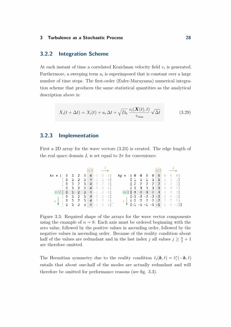
Figure 3.3: Required shape of the arrays for the wave vector componentsusing the example of n = 8: Each axis must be ordered beginning with thezero value, followed by the positive values in ascending order, followed by thenegative values in ascending order. Because of the reality condition abouthalf of the values are redundant and in the last index j all values j ≥ n

2+ 1

are therefore omitted.

The Hermitian symmetry due to the reality condition vi(k, t) = v∗i (−k, t)

entails that about one-half of the modes are actually redundant and will

therefore be omitted for performance reasons (see fig. 3.3).


Then one can generate Fourier modes as described in the previous chapter.

The central steps in the implementation are:

k = sqrt(kx **2 + ky **2)

# unit vector normal to k

ex , ey = -ky/k, kx/k

# generate amplitudes

c = sqrt( 4* pi* spectrum (k) / (k*l**2) )

# draw phases from a uniform distribution

phi = random . random (kx. shape )*2* pi

# generate Fourier modes

cvx , cvy = c * exp (1j*phi) * (ex , ey)

# modify zero column to ensure Hermitian symmetry

cvx [ -1:n/2: -1 ,0] = conj(cvx [1:n/2: ,0])

cvy [ -1:n/2: -1 ,0] = conj(cvy [1:n/2: ,0])

Here numpy’s vectorisation feature was used, i. e. all quantities which are

arithmetically related to the arrays kx/ky form arrays of the same shape and

the calculations are performed component-by-component.

Then for both components the complex-to-real transform is performed and

the real space velocity fields are generated:

cdata [:] = cvx | cdata [:] = cvy

c2r. execute () | c2r. execute ()

rvx = rdata .copy () | rvy = rdata .copy ()

3.2.4 Choice of the Parameters and Convergence

Choice of the Parameters There are different parameters/functions that

determine the flow properties and must be set initially.

The first parameter to be set is the number of Fourier modes N per dimension.

The higher this value, the higher is the resolution of the velocity fields and

hence the accuracy of the results. However, the creation of velocity fields

by means of a discrete Fourier transform is the bottleneck of the simulation.


Therefore, an upper limit for N is given by the available computer power

and simulation time. It turns out that values in between 256 and 2048 –

depending on the number of iterations – provide a good compromise.

Then a specific spectrum must be chosen. I use a Kolmogorov 5/3 spectrum

(see appendix B for a comparison of different spectra and their modelling).

The dissipative length scale κη must be chosen small enough such that the

missing Fourier modes beyond ±N/2 make a negligibly small contribution.

The integral length scale kLint defines the energy containing range. Ideally,

it is set to a rather small value such that there is a large inertial range in

between Lint and η. But if it is chosen to be too small, then only a few modes

contribute to the velocity field and the desired properties such as Gaussianity

and isotropy are not necessarily fulfilled.

Finally the choice of the parameters D0 and ui determines the relative strength

of the sweeping and the Kraichnan velocity field.

Convergence The Euler-Maruyama scheme is only of first order and hence

the integration step size must be quite small. Higher-order schemes are possible

but more difficult to realise than for deterministic differential equations. For

this thesis the Euler-Maruyama scheme works fine since the numerical results

only serve as a validation of the analytical ones (no quantitative information

is solely computed numerically) and the computational cost of quite small

time steps is manageable. However, when a quantitative accuracy is more

important, a higher-order scheme should be used (see [Ste13, ch. 5.6, 9]).

Another convergence problem is related to the ensemble averaging: In the

calculations there appear terms which are assumed to be of vanishing mean

(e. g. expressions including 〈 vi 〉). However, in some cases (depending on the

choice of parameters) their variance is still way larger than the mean values of

other non-vanishing terms. In that case it takes extremely many realisations

until the contribution of the former terms becomes negligible compared to

the non-vanishing ones and the convergence is really slow. Depending on the

situation, it might however be possible to adapt some of the parameters in

order to achieve a faster convergence.

4 Results 31

4 Results

In this chapter the dispersion of Lagrangian particles is analysed quantitatively

in a Kraichnan flow with an additional sweeping term. The cases under

consideration are the displacement of a single particle, the change in relative

separation of two distinct particles as well as a quantity that compares the

average distance of two particles at two different times for a given initial

distance. These quantities are initially calculated analytically and the results

are then compared with numerical Lagrangian simulations.

In the calculations two different averages are used: The first one is denoted by

simple angle brackets and implies averaging over a blob of fluid that is swept

around with a constant sweeping velocity. The second average is labelled by a

subscript ’sw’ which implies an additional average over many such blobs.

An initial qualitative impression of what is going on in this model can be

obtained from a sample dispersion of a blob of particles:

t = 0 t = 4 t = 8 t = 12

t = 16 t = 20 t = 24 t = 28

Multi-Particle Dispersion

Figure 4.1: Dispersion of a blob of fluid particle within the Kraichnan model.The red point indicates the motion of the center of mass.

4.1 Single-Particle Dispersion

The most simple statistical Lagrangian quantities are the mean and the mean-

squared displacement of a single particle. Let Xi(t0) be the particle’s initial

4 Results 32

position. Then the average displacement until some time t1 is given by:

〈 Xi(t1) − Xi(t0) 〉 (3.18)=

⟨ ∫ t1

t0

vi(X(t), t) dt +∫ t1

t0

ui(t) dt⟩

=∫ t1

t0

〈 vi(X(t), t) 〉︸︷︷︸

(3.19)= 0

dt +∫ t1

t0

〈 ui(t) 〉 dt

(3.15)=

ui (t1 − t0) t1 − t0 ≪ τsw

0 t1 − t0 ≫ τsw

(4.1)

When averaging over a single blob of fluid, the mean particle displacement

is independent of the turbulent Kraichnan velocity field as it is of vanishing

mean. On intermediate time scales one finds trivially a simple translation with

constant sweeping velocity ui. Under time scales which are large compared to

τsw the blob is swept around by many different velocities ui and the overall

contribution of the sweeping vanishes too. Then a particle’s current position

is the average position for all future times.

One can proceed analogously to compute the mean-squared displacement:

⟨

[Xi(t1) − Xi(t0)]2⟩ (3.18)

=

⟨[∫ t1

t0

vi(X(t), t) dt +∫ t1

t0

ui(t) dt]2⟩

=∫∫ t1

t0

〈 vi(X(t), t) vi(X(t′), t′) 〉︸︷︷︸

(3.20)= D0 ξii(X(t′)−X(t)) δ(t−t′)

dt dt′+

∫∫ t1

t0

〈 ui(t) 〉〈 vi(X(t′), t′) 〉︸︷︷︸

(3.19)= 0

dt dt′ +∫∫ t1

t0

〈 ui(t) ui(t′) 〉 dt dt′

(3.17)= d D0 (t1 − t0) +

u2 (t1 − t0)2 t1 − t0 ≪ τsw

d Dsw (t1 − t0) t1 − t0 ≫ τsw

(4.2)

Here the Einstein notation is implied (and responsible for the appearance of

the factor d stemming from the summation over δij). In contrast to the mean

4 Results 33

displacement, the mean-squared displacement is affected by the Kraichnan

flow as well (in a diffusive manner). One observes three different types of

motion depending on the time scale:

• small times:

Within small time increments the behaviour is dominated by the diffusive

Kraichnan motion (with diffusivity D0).

• intermediate times:

On times t1 with t1−t0 & D0/u2 the ballistic motion due to the sweeping

becomes dominant.

• large times:

The long-time behaviour t1 − t0 ≫ τsw becomes diffusive again with the

sweeping diffusivity Dsw.

0 200 400 600 800 1000

t

−50

0

50

100

150

200

250

300

Xi(t)−

Xi(0)

(a) Trajectories

100 101 102 103

t

10−1

100

101

102

103

104

105

⟨

[Xi(t)−

Xi(0)]2⟩

(b) Mean-Squared Displacement

2D0 t+ u2 t2

2D0 t

u2 t2

simulation

Single-Particle Dispersion

Figure 4.2: Lagrangian simulation of single-particle dispersion (a) In the leftplot some sample trajectories are shown. They exhibit a diffusive behavioursuperimposed by a linear drift. (b) In the right plot the green dashed lineindicates the mean-squared displacement as computed by averaging over 2 500Lagrangian trajectories for small and intermediate time intervals. The otherlines show the theoretical predictions for time scales on which the sweepingis assumed to be constant. The choice of the parameters was D0 = 1 andux = uy = 0.2.

4 Results 34

The calculations so far were related to individual blobs with constant sweeping

velocity. Additional averaging over many such blobs with different sweeping

velocities gives:

〈 Xi(t1) − Xi(t0) 〉sw = 0 (4.3)

⟨

[Xi(t1) − Xi(t0)]2⟩

sw= d D0 (t1 − t0) (4.4)

+ u2rms

(t1 − t0)2 t1 − t0 ≪ τsw

τsw (t1 − t0) t1 − t0 ≫ τsw

Comparison with Other References In real turbulence the root-mean-

squared displacement is expected to follow ∼√

t with the square root of the

diffusivity as the constant of proportionality. This coincides with the motion

generated by the Kraichnan ensemble. However, in real turbulence there is

also a ballistic regime for very small times which is caused simply by the

temporal smoothness of the velocity (the velocity field can be considered as

being almost constant on such time scales) [MY75, ch. 9.3]. This effect does

not show up in our result as we are dealing with delta-correlated fields which

remain diffusive for arbitrarily small time scales.

4.2 Two-Particle Dispersion

The next interesting Lagrangian quantity is the two-particle dispersion, i. e.

the evolution of the distance of two distinct particles (within the same blob of

fluid). Let the particles be indicated by superscripts (a) and (b) respectively

and let the components of the separation vector be denoted by

Ri(t) := X(b)i (t) − X

(a)i (t) . (4.5)

The calculation of the mean and the mean-squared relative displacement

works analogously to the case of the single-particle dispersion:

4 Results 35

〈 Ri(t1) − Ri(t0) 〉 (3.18)(4.5)= (4.6)

⟨∫ t1

t0

vi(X(b)(t), t) dt +

✟✟

✟✟

✟✟∫ t1

t0


particle (b)

−∫ t1

t0

vi(X(a)(t), t) dt −

✟✟✟✟✟✟∫ t1

t0


particle (a)

⟩

(3.19)=

∫ t1

t0

⟨

vi(X(b)(t), t)

⟩

︸︷︷︸

=0

dt −∫ t1

t0

⟨

vi(X(a)(t), t)

⟩

︸︷︷︸

=0

dt = 0

⟨

[Ri(t1) − Ri(t0)]2⟩ (3.18)(4.5)

=

⟨[∫ t1

t0

vi(X(b)(t), t) dt −

∫ t1

t0

vi(X(a)(t), t) dt

]2⟩

(3.19)(4.5)=

∫∫ t1

t0

⟨

vi(X(b)(t), t) vi(X

(b)(t′), t′)⟩

︸︷︷︸

d D0 δ(t−t′)

dt dt′

− 2∫∫ t1

t0

⟨

vi(X(b)(t), t) vi(X

(a)(t′), t′)⟩

︸︷︷︸

D0 ξii(X(b)(t)−X

(a)(t′)) δ(t−t′)

dt dt′

+∫∫ t1

t0

⟨

vi(X(a)(t), t) vi(X

(a)(t′), t′)⟩

︸︷︷︸

d D0 δ(t−t′)

dt dt′

(3.20)= 2D0

[

d (t1 − t0) −∫ t1

t0

ξii(R(t)) dt]

(4.7)

Again, the Einstein notation is implied and causes the appearance of d. The

evolution of the mean-squared distance can be expressed more compactly in

differential form:

d

dt

⟨

R2(t)⟩

= lim∆t→0

〈 R2(t + ∆t) − R2(t) 〉∆t

= 2D0 [d − ξii(R(t))] (4.8)

The (simultaneous) two-point statistics are independent of the sweeping as the

sweeping affects both particles equally. Hence they depend on the Kraichnan

4 Results 36

flow only. The rate of change of the squared separation ddt

〈 R2i (t) 〉 of two

Lagrangian particles is a function of that distance R(t) by virtue of the

correlation tensor ξii(R(t)) of the Kraichnan ensemble.

In the limit of R(t) → 0 the elements on the principal diagonal of the velocity

correlation tensor ξii(R(t)) approach 1 (and the trace becomes equal to d)

such that the particles’ separation is found to remain constant in that limit

(see (4.8)):

d

dt

⟨ [

X(b)i (t) − X

(a)i (t)

]2⟩

≈ 0 (4.9)

On the other hand, for large distances R(t) the velocities become completely

uncorrelated (ξii(R) ≈ 0) and the change in the particles’ separation behaves

as in a purely diffusive case:

d

dt

⟨ [

X(b)i (t) − X

(a)i (t)

]2⟩

= 2D0 d (4.10)

The behaviour in between these extreme cases depends on the specific shape of

the correlation tensor ξij (and hence on the underlying energy spectrum).

Literature Most of the available literature is concerned with the inertial

range dispersion only. A recent paper that deals with the particle dispersion

in kinematic simulations of turbulence is [TD05]. It states that different such

kinematic simulations support a particle separation law that goes like

⟨

Ri(t)2⟩

∼ t3 (4.11)

in the inertial range. Hence, its temporal derivative is expected to be propor-

tional to t2. This seems to coincide with our result (dashed grey line in fig.

4.3) for the inertial subrange (given by R ≪ Lint which was set to Lint ≈ 0.08

in the simulation).

4 Results 37

0.00 0.05 0.10 0.15 0.20

R(t)

0

1

2

3

4

5

d dt

⟨

R(t)2⟩

2D0 [ 2− ξii(R(t)) ]

intertial range fit ∼ R(t)2

4D0

Lagrangian simulation

Two-Particle Dispersion

Figure 4.3: Differential change of the squared separation of two particles: Thesimulation results (green bullets) were computed by averaging over (250 000)Lagrangian increments for various initial separations R in a 2D flow (d = 2).One observes that the diffusivity (rate of separation) strongly depends on thespacing of the particles. Its specific dependence is determined by the choiceof the energy spectrum.

4.3 Two-Time Two-Particle Dispersion

An even more general quantity is the correlation of the position of two

particles (a) and (b) at two different times t1 and t2 with a given initial

distance Ri(t0) = X(b)i (t0) − X

(a)i (t0). Then the mean and the mean-squared

distances are given by:

⟨

X(b)i (t2) − X

(a)i (t1)

⟩

(4.12)

=⟨

X(b)i (t1) +

∫ t2

t1

ui dt +∫ t2

t1

vi(X(b)(t), t) dt − X

(a)i (t1) dt

⟩

= 〈 Ri(t1) 〉︸︷︷︸

(4.7)= Ri(t0)

+ui (t2 − t1) +∫ t2

t1

⟨

vi(X(b)(t), t)

⟩

︸︷︷︸

=0

dt

= Ri(t0) + ui (t2 − t1)

4 Results 38

⟨ [

X(b)i (t2) − X

(a)i (t1)

]2⟩

(4.13)

=

⟨[

X(b)i (t1) +

∫ t2

t1

ui dt +∫ t2

t1

vi(X(b)(t), t) dt − X

(a)i (t1) dt

]2⟩

=⟨

R2(t1)⟩

︸︷︷︸

two-particle disp. in (t0,t1)

+ 2 〈 Ri(t1) 〉︸︷︷︸

=Ri(t0)

ui(t2 − t1) + d D0 (t2 − t1) + u2(t2 − t1)2

︸︷︷︸

single-particle dispersion of (b) in (t1,t2)

One basically observes an combination of a two-particle dispersion in the time

interval (t0, t1) and an additional single particle dispersion in the time interval

(t1, t2) caused by the particle (b) which keeps moving in that additional

time interval. The remaining term 2Ri(t0) ui(t2 − t1) can be interpreted as

follows:

(a) (b)R(t0)

(b) (a)R(t0)

u

Figure 4.4: As the motion of particle (b) is observed for a longer time thanparticle (a), the relative orientation of their initial separation vector r(t0) withrespect to the sweeping velocity vector u actually matters in the sense thatthe sweeping during (t1, t2) either tends to reduce the particles’ separation(for opposite orientation) or to increase (otherwise).

It takes account for the relative orientation of the initial separation vector

Ri and the direction of the sweeping ui. If these are oriented in opposite

directions, then (because of the additional motion of particle (b) during

(t1, t2)) the term tends to reduce the particles’ distance somewhat whereas it

otherwise (on average) tends to drive apart them even more.

Additional averaging over the ensemble of sweeping velocities ui eliminates

the additional cross term and only the contributions from the two-particle

dispersion during (t0, t1) and the single-particle dispersion during (t1, t2)

4 Results 39

remain:

⟨

X(b)i (t2) − X

(a)i (t1)

⟩

sw= Ri(t0) (4.14)

⟨ [

X(b)i (t2) − X

(a)i (t1)

]2⟩

sw= R2(t1) + d D0 (t2 − t1) + u2

rms(t2 − t1)2

(4.15)

The simulation (see fig. 4.5) confirms the analytical result in eq. (4.14) quite

well, even though slight deviations are visible.

100 101 102 103

t2 − t1

10−1

100

101

102

⟨

[

X(b)

i(t

2)−X

(a)

i(t

1)]

2⟩

theory

simulation⟨

R2(t1)⟩

2 (Ri(t0)ui +D0) (t2 − t1)

u2 (t2 − t1)2

Two-Time Two-Particle Dispersion

Figure 4.5: Exemplary numerical result for the correlation of the squaredseparation of two particles at two different times t1 and t2 for fixed time t1 andfixed initial separation vector Ri(t0). The ensemble average was performedover 10 000 realisations.

5 Conclusion 40

5 Conclusion

5.1 Summary of the Results

Description of the Kraichnan Model

Recall that the Kraichnan model was defined as follows: The velocities are

assumed to be Gaussian with well-defined statistics

〈 vi 〉 = 0 (5.1)

〈 vi(x, t) vj(x + r, t′) 〉 = v2rmsξij(r) δ(t − t′) (5.2)

with ξij being the normalised spatial velocity correlation function.

In the Lagrangian description the trajectories are then given by integral

equations such as:

∆Xi(t) =∫

vi(X(t), t) dt (5.3)

One of the major obstacles in this thesis was to achieve a proper understanding

of the Kraichnan model in terms of stochastic calculus. The obscure questions

were:

• What is the interpretation of delta-correlated velocities as they are

actually infinite? How are integrals like (5.3) properly defined whilst

the integrand is infinite and nowhere differentiable?

• How can these infinite, non-differentiable velocities be related to finite

velocity statistics (e. g. given by the energy spectrum) and implemented

numerically?

These question were resolved in chapter 3.1 by describing the Kraichnan model

as the limit of a finite-correlation time process with correlation time τ : In this

case velocities are still finite and can be interpreted in the classical sense. A

delta-correlated process is then achieved in the limit of zero correlation time.

5 Conclusion 41

If this limiting process is being accompanied by a simultaneous rescaling of

the velocity field in such fashion that the diffusivity – defined as

D0 := v2rmsτ (5.4)

– remains constant, the long time displacement statistics are unaffected. It

was derived before that the motion on time scales large compared to τ is

solely characterised by this quantity.

It was then seen that a meaningful interpretation of integrals like (5.3) is

achieved by subsequent averaging and application of (5.1) and (5.2) to the

averaged integrands.

Furthermore, it was demonstrated that the numerical integration scheme

∆Xi(t) =√

D0vi(X(t), t)

vrms

√∆t (5.5)

generates a behaviour in accordance with the analytical description of the

delta-correlated process and can be used for a numerical simulation.

Finally the physically motivated description of the Kraichnan model (in terms

of velocities) was linked to the mathematical description in terms of stochastic

calculus (similar to the extensively studied Brownian motion case):

As the velocities are assumed to be normally distributed, the expression

vi/vrms is simply a Gaussian random number of variance 1 and its product

with√

∆t describes a standard Wiener process ∆Wi(X(t), t). The Lagrangian

increments are then given by:

∆ Xi(t) =√

D0 ∆ Wi(X(t), t) (5.6)

This looks familiar to the Brownian motion case except for the spatial cor-

relation of the velocity field. But that restriction can be included by a

corresponding correlation of the individual Wiener processes.

It is zero for non-overlapping time intervals (because of the independence of

5 Conclusion 42

the increments in a Wiener process) and

〈 ∆Wi(X(t), t) ∆Wj(X′(t), t) 〉 =

∫

ξij(X′(t) − X(t)) dt (5.7)

on coinciding time intervals.

Dispersion of Lagrangian Particles

Single-Particle Dispersion The delta-correlated Kraichnan velocity field

causes – just like real turbulence – a diffusive motion with diffusivity D0 and

root-mean-squared displacement that goes with√

t. The diffusive motion

is the dominant action on small time scales. However, in real turbulence

there is always a ballistic regime for very small time scales simply due to the

smoothness of the velocity field. It is missing in the Kraichnan model as the

velocity field is not smooth in that case but varying infinitely rapidly [MY75,

ch. 9.3].

The additional random sweeping term generates a ballistic translation and

its contribution to the root-mean-squared displacement is linear in time.

Therefore it is initially negligible compared to the diffusive motion but it

becomes the dominant contribution on larger time scales.

The time of the transition depends on the ratio of the amplitudes D0 and

u2rms and is given by

ttrans ≈ D0

u2rms

. (5.8)

If one assumes that the sweeping is only constant over a time interval τsw

and then changes its direction randomly, the motion on time scales ≫ τsw

becomes diffusive again with diffusivity

Dsw = u2rms τsw. (5.9)

5 Conclusion 43

log⟨∆X2(t)

⟩

diffusiveballistic

diffusive

log tDsw/u2rmsDKr/u2

rms

Single-Particle Dispersion

Kraichnanmotion

sweeping sweeping

Figure 5.1: On small time scales the single-particle dispersion is dominatedby the diffusive Kraichnan motion. On intermediate time scales the ballisticmotion due to the sweeping becomes dominant as long as the approximation ofconstant sweeping is valid. On the long run the sweeping changes it directionitself multiple times and hence the long time behaviour becomes diffusiveagain.

Two-Particle Statistics The simultaneous two-particle statistics are inde-

pendent of the random sweeping as both particles are affected equally and

therefore only the Kraichnan motion causes a relative displacement of the

particles.

The rate of change of separation ddt

〈 R2(t) 〉 of two Lagrangian particles

depends then on the correlation of their velocities and hence their distance

R(t):

d

dt

⟨

R2(t)⟩

= 2D0 [d − ξii(R(t))] (5.10)

Here ξii is the trace of the normalised spatial correlation tensor. In the limit of

vanishing distance the term in square brackets becomes zero and the particles’

separation does not change at all. On the other hand, for sufficiently large

distances the velocities become completely uncorrelated and ξii(R(t)) = 0.

Then the particles’ relative separation increases at a constant rate 2 D0 d as

if the particles were simply in an uncorrelated diffusive motion.

5 Conclusion 44

Two-Time Two-Particle Statistics The correlation of two particle’s posi-

tion at different times t1 and t2 is in general a function of both these times

as well as the initial separation vector Ri(t0). The mean distance of these

particles at different times t0 and t1 is for the most part given by a term that

accounts for a simple two-particle dispersion in the time interval (t0, t1) as

well as a single particle dispersion in the time interval (t1, t2).

Furthermore, there appears an additional cross term in the mean-squared

quantity that accounts for the relative orientation of the initial separation

vector Ri(t0) and the sweeping direction given by ui. However, when averaging

over the ensemble of sweeping velocities, this contribution is eliminated.

5.2 Evaluation of the Methods

The Kraichnan Model The great advantage of the Kraichnan model is

that it is a model which is completely analytically tractable. This is a

property which is rather rare in the area of turbulence research. However,

this tractability is based on two unrealistic assumptions, namely the delta-

correlation in time and the Gaussianity of the velocity field (see also [Dav04,

ch. 5.5]: ’Why turbulence is never Gaussian’). So how meaningful is such a

model after all?

Initially, it attracted only little attention for being based on such unrealistic

assumptions. However, it experienced a revival during the nineties as it was

realised that this model was able to generate so-called intermittent behaviour

(deviations from the Gaussianity of specific probability distributions even

though it uses Gaussian velocity fields). This intermittency had been identified

before as one of the most crucial deviations of the – otherwise very successful

– K41 theory from experimental observations [Kra94]. This shows that even

unrealistic assumptions can generate striking insights.

Furthermore, one can consider the Kraichnan model as just a different ap-

proach to the turbulence problem: Instead of trying to make physically correct

equations analytically tractable one can just as well start from an analytically

5 Conclusion 45

tractable (but unrealistic) model and eventually try to make the model more

and more realistic (e. g. by introducing finite time correlations) while keeping

the analytical tractability.

Moreover, the Kraichnan model opens the door for a description of turbulence

in terms of stochastic calculus. Thereby an additional class of mathematical

tools becomes available for tackling the turbulence problem.

Numerical Implementation One of the flaws of the numerical implemen-

tation of the Kraichnan model in this thesis is the slow convergence of the

integration scheme. This requires quite small step sizes. In this thesis the

numerical calculations were intended to be used only qualitatively as a cross

check of the analytical results. No quantitative results were computed solely

numerically.

In situations where quantitative numerical results are required one should be

more concerned with error estimations and try to improve the convergence of

the computation, e. g. by using a higher-order integration scheme (see [Ste13,

ch. 5.6, 9]).


A Eulerian Description of the Kraichnan Flow

In this thesis the physical behaviour was examined in the Lagrangian picture

but one can just as well work in the Eulerian picture which will be derived

in the following. The calculations are guided by similar ones in [CFG08, ch.

2]

Consider any scalar field ϑ(x, t) with initial distribution ϑ0(x0, t0), subject

to a Kraichnan velocity field vi(x, t) superimposed by a large-scale random

sweeping term ui.

Link Between the Lagrangian and Eulerian Description The Eulerian

description can be derived from the Lagrangian one. Both descriptions are

linked by the following equation: [CFG08, ch. 2.2.3]

ϑ(x, t) =∫

〈 δ(x − X(t; x0)) 〉 ϑ(x0, t0) dx0 (A.1)

The Eulerian field ϑ(x, t) is made up of contributions from all Lagrangian

trajectories with X(t; x0) = x (here X(t; x0) means that X(t0; x0) = x0).

During the following derivations the arguments (t; x0) might be omitted here

and there for the sake of clarity.

Each of these trajectories contributes with the amount ϑ0(x0, t0) that was

initially assigned to them. However, the trajectories are not deterministic

but stochastic processes. A proper evaluation which takes account of this

probability distribution is ensured by the ensemble average 〈 · 〉.

Time Evolution Now the objective is to derive an expression for the time

evolution ∂t ϑ(x, t) of the scalar field.

∂t ϑ(x, t) = ∂t

∫

〈 δ(x − X(t; x0)) 〉 ϑ(x0, t0) ddx0

︸︷︷︸

ϑ(x,t)

(A.2)

The only quantity with explicit time dependence (and affected by the time

derivative) is the delta function. To evaluate this distributional derivative,


both sides are multiplied by some arbitrary test function ξ(x) and integrated

over space:

∫

ξ(x) ∂t ϑ(x, t) ddx

︸︷︷︸

:=LHS

=∫

∂t

⟨∫

ξ(x) δ(x − X(t; x0)) ddx

︸︷︷︸

=ξ(X(t;x0))

⟩

ϑ(x0, t0) ddx0

(A.3)

LHS =∫

〈 ∂t ξ(X(t; x0)) 〉 ϑ(x0, t0) ddx0 (A.4)

This expression involves a derivative of a function of the stochastic process

X(t). For the evaluation one can use a theorem from stochastic calculus

which is called Ito’s lemma (it will be derived for this case now): [Pop00, p.

722]

Ito’s Lemma

Consider a multivariate Taylor expansion of ξ(X(t; x0)):

∆ξ(X(t)) := ξ(X(t + ∆t)) − ξ(X(t)) (A.5)

≈✘✘✘✘✘✘

∂t ξ(X(t)) ∆t + ∂Xiξ(X(t)) ∆Xi

+1

2∂Xi

∂Xjξ(X(t + ∆t)) ∆Xi ∆Xj + O

(

∆t3/2)

The increments ∆Xi are given by the Langevin equation:

∆Xi(t) = ui ∆t +∫ t+∆t

tvi(X(s), s) ddt (A.6)

Averaging and application of the conditions

〈 vi 〉 = 0 (A.7)

〈 vi(X(t), t) vj(X(t′), t′) 〉 = Dij(X(t′) − X(t)) δ(t − t′) (A.8)


with Dij(0) := D0 yields:

d

dt〈 ξ(X(t)) 〉 = lim

∆t→0

1

∆t[ξ(X(t + ∆t)) − ξ(X(t))]

= ui 〈 ∂Xiξ(X(t)) 〉 +

1

2D0

⟨

∂2ξ(X(t))

∂Xi2

⟩

. (A.9)

End Ito’s Lemma

With this result, the calculation (eq. (A.4)) can be continued:

LHS =∫ [

ui 〈 ∂Xiξ(X) 〉 +

1

2D0

⟨

∂2Xi

ξ(X)⟩]

ϑ(x0, t0) ddx0 (A.10)

Next one can insert a 1 =∫

δ(x − X(t; x0)) ddx in order to eliminate ξ:

LHS =∫ [

ui

⟨

∂Xi

∫

δ(x − X(t; x0)) ξ(X(t; x0)) ddx

⟩

+1

2D0

⟨

∂2Xi

∫

δ(x − X(t; x0)) ξ(X(t; x0)) ddx

⟩]

ϑ(x0, t0) ddx0

=∫∫

ξ(x) [ui 〈 ∂Xiδ(x − X(t; x0)) 〉

+1

2D0

⟨

∂2Xi

δ(x − X(t; x0))⟩]

ϑ(x0, t0) ddx0 dd

x (A.11)

Furthermore,

∂

∂Xi

=∂(xi − Xi)

∂Xi

∂

∂(xi − Xi)= −∂(xi − Xi)

∂xi

∂

∂(xi − Xi)= − ∂

∂xi

such that the derivatives can be replaced as follows:

LHS =∫∫

ξ(x) [−ui ∂xi〈 δ(x − X(t; x0)) 〉

+1

2D0 ∂2

xi〈 δ(x − X(t; x0)) 〉

]

ϑ(x0, t0) ddx0 dd

x


Now, using eq. (A.1) again yields

LHS =∫

ξ(x)

−ui ∂xi

∫

〈 δ(x − X(t; x0)) 〉 ϑ(x0, t0) ddx0

︸︷︷︸

=ϑ(x,t)

(A.12)

+1

2D0 ∂2

xi

∫

〈 δ(x − X(t; x0)) 〉 ϑ(x0, t0) dx0

︸︷︷︸

=ϑ(x,t)

ddx

such that one ends up with:

∫

ξ(x) ∂t ϑ(x, t) ddx =

∫

ξ(x)[

−ui ∂xiϑ(x, t) +

1

2D0 ∂2

xiϑ(x, t)

]

ddx

As ξ was assumed to be an arbitrary test function, the remaining integrands

must be equal, too. This finally yields an advection-diffusion equation with

drift ui and diffusivity D0

⇔ ∂t ϑ(x, t) + ui ∂xiϑ(x, t) − 1

2D0 ∂2

xiϑ(x, t) = 0 (A.13)


B Energy Spectrum of Real Flows

For a quantitative description of the energy spectrum E(κ) of real turbulent

flows, Kolmogorov developed a theory based on Richardson’s energy cascade

model:

3D Inertial Range As was mentioned before, in a 3D turbulent flow one

observes two characteristic length scales: The integral scale Lint which is the

characteristic macroscopic scale of turbulence and the dissipative scale η at

which the kinetic energy is removed from the system by means of viscous

dissipation. Kolmogorov suggested that in between these scales (i. e. in

the inertial subrange) the energy is transferred from the large scales to the

dissipative scales successively and at a constant rate per unit mass ε. The

mechanism behind this energy transfer is the decay of large eddy structures

to smaller ones (called direct energy cascade).

Kolmogorov assumed that statistical properties of a turbulent flow are univer-

sal in the inertial range and characterised solely by the rate of energy transfer

ε. Based on this assumption he derived an expression for the turbulent energy

spectrum by using dimensional analysis [Pop00, ch. 6.5.2]:

E(κ) = CK ε2/3 κ−5/3 (B.1)

Here CK is a non-dimensional constant (nowadays referred to as Kolmogorov

constant) and κ is the wave number that defines the length scale. This result

is found to be in quite good accordance with experimental results [DPR03,

ch. 2.1].

2D Inertial Range In 2D turbulence the picture is not as clear as in three

dimensions. One reason is that there is actually no such thing as purely

two-dimensional turbulence in reality. Every set-up – no matter how sophisti-

cated – is ultimately of finite thickness and hence three-dimensional. So for

purely two-dimensional turbulence one is left with theoretical or numerical

approaches.


One of the first theoretical approaches to 2D turbulence was done by Kraich-

nan. He found that the 2D energy spectrum exhibits significant qualitative

differences to the 3D case: in two-dimensional turbulence not only the rate

of energy dissipation but also the rate of enstrophy (mean-squared vorticity

[Pop00, ch. 2.7]) transfer is a constant of motion. This implies that yet

another inertial range becomes possible, namely one with constant enstrophy

transfer. Furthermore, the energy cascade is reversed: It is now directed

from the small scales towards the large scales (from large to small wave

numbers). If there is no large-scale dissipation mechanism, then the total

energy of the system increases incessantly and the integral length scale is

shifted to smaller and smaller wavelengths. The enstrophy transfer is however

directed towards the small scales (large wave numbers) and gives rise to a

direct cascade [Kra67]. Computer simulations have recently proven a good

agreement with this theory [BKSB09].

inertial range

log κLint log κη log κ

log E

log κLint log κη log κ

log E

forcing

energyenstrophy

(a) 3D Spectrum (b) 2D Spectrum

energy

Figure B.1: Qualitative shape of the energy spectrum in turbulent flows. Inthe 3D case the forcing occurs at some integral length scale Lint and one findsa direct energy cascade towards the small scales. The picture is different in2D: At some band of wavelengths κ the system is forced, i. e. the energy andenstrophy is fed into the system. One observes a direct enstrophy cascade anda reversed energy cascade. The numbers indicate the power law exponents inthe respective intervals.

Beyond the Inertial Range Outside the inertial range the spectrum is

assumed to obey the following laws: [Pop00, ch. 6.5.3][Dav04, chs. 6.3.1 and

6.3.5]

• κ << κLint : E(κ) ∼ κp0


with p0 being either 2 or 4 in 3D and 3 in 2D. Here κLint = 2π/Lint

corresponds to the integral length scale, i. e. the length scale at which

energy is pumped into the system.

• κ >> κη: E(κ) ∼ e−βκ

with β being an experimental constant. κη = 2π/η corresponds to

the dissipative length scale, i. e. the scale where the kinetic energy is

dissipated into internal degrees of freedom by means of viscosity.

Model Spectrum A composite spectrum that includes all length scales can

be modelled as a product of various terms which are constructed such that

each of them exhibits the characteristic behaviour in one of the three ranges

while the other ones remain undisturbed. When using the -5/3 spectrum it

reads

E(κ) = Ck ε2/3 κ−5/3 fLint(κLint) fη(κη) (B.2)

with

fLint(κL) =

(

κLint

[(κLint)2 + cL]1/2

)5/3+p0

(B.3)

fη(κη) = exp(

−β 4

√

(κη)4 + c4η − cη

)

(B.4)

The experimental value for the decay coefficient is β ≈ 5.2. The fit parameters

cL and cη are determined such that E(κ) and 2νκ2E(κ) integrate to the total

energy and the dissipation rate ε of the system. These requirements are found

to be met for cL ≈ 6.78 and cη ≈ 0.40 [Pop00, ch. 6.5.3]. The quantities ε,

Lη and Lint can be chosen according to the specific physical set-up.


0 50 100 150 200

k

0.0

0.2

0.4

0.6

0.8

1.0

E(k)

ǫ = 50

ǫ = 200

ǫ = 600

ǫ = 1200

101 102 103

k

10−4

10−3

10−2

10−1

100

101

(a) Dissipation Rate

0 50 100 150 200

k

0.0

0.2

0.4

0.6

0.8

1.0

E(k)

η = 2π/1000

η = 2π/2000

η = 2π/4000

η = 2π/8000

101 102 103

k

10−4

10−3

10−2

10−1

100

101

(b) Dissipative Length Scale

0 50 100 150 200

k

0.0

0.2

0.4

0.6

0.8

1.0

E(k)

L = 2π/20

L = 2π/30

L = 2π/50

L = 2π/80

101 102 103

k

10−4

10−3

10−2

10−1

100

101

(c) Integral Length Scale

Figure B.2: Here the model spectrum is plotted for several variations of itsparameters ε (rate of energy dissipation), η (dissipative length scale) and Lint

(integral length scale).


C Validation of the Numerical Velocity Fields

Figure C.1: Plot of the absolute value of a sample velocity field generatednumerically as described before.

In this subsection a couple of plausibility checks are described that have

been done in order to verify whether the numerically generated velocity fields

actually have the desired properties.

Gaussianity A characteristic feature of normally distributed random vari-

ables (with zero mean) is that the odd moments vanish and that the even mo-

ments are completely determined by the second moment [Bir13, ch. 2.7]:

⟨

v4i

⟩

= 3⟨

v2i

⟩2,

⟨

v6i

⟩

= 15⟨

v2i

⟩3,

⟨

v8i

⟩

= 105⟨

v2i

⟩4, . . . (C.1)

Hence, a way to verify the Gaussianity is to check these relations.

n 0 1 2 3 4 5 6 7 8

〈 vni 〉 1.000 0.000 0.899 -0.01 2.42 -0.1 11 -1 70

uncertainty 0.000 0.000 0.000 0.09 0.12 0.9 2 9 30

Table 4: First central moments 〈 vni 〉 of the numerically generated velocity

fields and the corresponding uncertainty in a two-stage averaging process. Ina Gaussian field the odd moments are supposed to vanish. The larger theorder the moment under consideration, the slower is the convergence undernumerical averaging as the increasing uncertainty clearly shows.


Therefore the first central moments of the velocity distribution have been

determined numerically (see table 4). A computation of the second moment

for each of the even moments according to eq. (C) yields:

n 0 1 2 3

〈 v2i 〉 0.899 ± 0.001 0.90 ± 0.08 0.9 ± 0.7 1 ± 8

Table 5: Calculation of the second moment for the first few even momentsaccording to eqs. (C).

Here, the Gaussianity is confirmed by the results as the relations are ful-

filled.

Histograms of the one-point velocity PDF and the velocity increment PDFs

for different increments serve as another validation of the Gaussianity of the

velocity field. As Gaussian PDFs are proportional to e−(x−µ)2/σ2, they are

supposed to appear as reversed parabolas in a log-normal plot, which appears

to be the case (see fig. C.2).

−2.0−1.5−1.0−0.5 0.0 0.5 1.0 1.5 2.0vi

−8

−6

−4

−2

0

logPDF

(a) One-Point PDF

histogram

theory

−2.0−1.5−1.0−0.5 0.0 0.5 1.0 1.5 2.0

vi(xi)− vi(xi + a L

n)

−5

−4

−3

−2

−1

0

1

2

(b) Two-Point PDF

a = 4a = 8

a = 16a = 32

Velocity Distribution Statistics

Figure C.2: (a) Double logarithmic plot of the one-point velocity distribu-tion histogram together with the theoretical expectation −v2

i /(2 v2rms). (b)

Distribution of velocity increments for different increments ∆xi = aLn. For

a Gaussian field one expects reversed parabolas for all probability densityfunctions in a loglog plot.


Incompressibility The incompressibility condition relates the longitudinal

and transverse correlation functions with each other. As was stated before

(eq. (2.7)), that relation reads in the 2D case:

g(r) = f(r) +f ′(r)

r(C.2)

So this condition can be used to numerically check if the velocity field is

incompressible:

0.0 0.2 0.4 0.6 0.8 1.0

r

−0.4

−0.2

0.0

0.2

0.4

0.6

0.8

1.0

1.2f(r) (longitudinal)

L = 2π/10 L = 2π/20 L = 2π/50 L = 2π/120

0.0 0.2 0.4 0.6 0.8 1.0

r

g(r) (transverse)

0.0 0.2 0.4 0.6 0.8 1.0

r

f(r) + f ′(r)/r − g(r)

Correlation Functions

Figure C.3: Longitudinal and transverse correlation functions of the numeri-cally generated velocity field.

Hence, incompressibility seems to be indicated as well.

References 57

References

[Ber00] D. Bernard. Turbulence for (and by) amateurs. arXiv preprint

cond-mat/0007106, 2000.

[Bir13] B. Birnir. The Kolmogorov-Obhukov Theory of Turbulence.

Springer, 2013.

[BKSB09] W. Bos, B. Kadoch, K. Schneider, and J. P. Bertoglio. Iner-

tial range scaling of the scalar flux spectrum in two-dimensional

turbulence. Phys. Fluids, 21(11):115105, 2009.

[CFG08] J. Cardy, G. Falkovich, and K. Gawedzki. Non-equilibrium sta-

tistical mechanics and turbulence. Cambridge University Press,

2008.

[CK89] S. Chen and R. H. Kraichnan. Sweeping decorrelation in isotropic

turbulence. Phys. Fluids A-Fluid, 1(12):2019–2024, 1989.

[Dav04] P. Davidson. Turbulence: An introduction for scientists and engi-

neers. Oxford University Press, 2004.

[DPR03] P. Durbin and B. Pettersson Reif. Statistical theory and modeling

for turbulent flows. John Wileys and Sons, 2003.

[FGV01] G. Falkovich, K. Gawedzki, and M. Vergassola. Particles and fields

in fluid turbulence. Rev. Mod. Phys., 73(4):913, 2001.

[FJ12] M. Frigo and S. Johnson. Fftw: Fastest fourier transform in the

west. ASCL, 1:01015, 2012.

[Fuc13] C. Fuchs. Inference for diffusion processes: With applications in

life sciences. Springer, 2013.

[Kra64] R. H. Kraichnan. Kolmogorov’s hypotheses and eulerian turbulence

theory. Phys. Fluids, 7(11):1723–1734, 1964.

[Kra67] R. H. Kraichnan. Inertial ranges in two-dimensional turbulence.

Phys. Fluids, 10(7):1417–1423, 1967.

References 58

[Kra68] R. H. Kraichnan. Small-scale structure of a scalar field convected

by turbulence. Phys. Fluids, 11(5):945–953, 1968.

[Kra94] R. H. Kraichnan. Anomalous scaling of a randomly advected

passive scalar. Phys. Rev. Lett., 72(7):1016, 1994.

[Les97] Lesieur, M. Turbulence in fluids. Kluwer Academic Publishers,

1997.

[Maz02] R. M. Mazo. Brownian motion: Fluctuations, dynamics, and

applications. Oxford University Press, 2002.

[MY75] A. S. Monin and A. M. Yaglom. Statistical fluid mechanics: Me-

chanics of turbulence. MIT Press, 1975.

[NT90] M. Nelkin and M. Tabor. Time correlations and random sweeping

in isotropic turbulence. Phys. Fluids A-Fluid, 2(1):81–83, 1990.

[Pop00] S. Pope. Turbulent flows. Camebridge University Press, 2000.

[Ric07] L. F. Richardson. Weather prediction by numerical process. Cam-

bridge University Press, 2007.

[SS92] T Sanada and V Shanmugasundaram. Random sweeping effect in

isotropic numerical turbulence. Phys. Fluids A-Fluid, 4(6):1245–

1250, 1992.

[Ste13] S. Stepanov. Stochastic world. Springer, 2013.

[TD05] D.J. Thomson and B.J: Devenish. Particle pair separation in

kinematic simulations. J. Fluid Mech., 526:277–302, 2005.

[Ten75] H. Tennekes. Eulerian and lagrangian time microscales in isotropic

turbulence. J. Fluid Mech., 67:561–567, 2 1975.

bachelor thesis impact of random sweeping and turbulent ... · bachelor thesis impact of random...

Documents