b. · the theory and analysis of diallel crosses* b. i. hayman a .r. c. unit of biometrical...

THE THEORY AND ANALYSIS OF DIALLEL CROSSES*

B. I. HAYMAN

A .R. C. Unit of Biometrical Genetics, Department of Genetics, University of Birmingham

Received January 28, 1954

I. INTRODUCTION

T H E diallel cross method of investigating the genetical properties of a group of homozygous lines has recently received much attention. HULL

(1945) has considered some aspects of the method. A short summary of a more general approach by JINKS and HAYMAN (1953) and its application to several published sets of maize data has also appeared. In another paper JINKS (1954) has described experiments on inbred lines of Nicotina rustica, and has given an account of some of the associated statistics together with a discussion of the results. In this paper we apply a genetic algebra to the theory of the diallel cross, not only to re-establish the formulae of JINKS, but also to investigate more complex genetical systems. We will show how to measure additive and dominance variation, how to describe the relative dominance properties of the parental lines and how to detect non-allelic genic interaction. A ivorked example illustrates the theory.

The following definitions will be used. A diallel cross is the set of all possible matings between several genotypes. The genotypes may be defined as individuals, clones, homozygous lines, etc., and, if there are n of them, there are n2 mating combinations, counting reciprocals separately. A diallel table is an arrangement in a square of n2 measurements corresponding one-to-one to the mating combinations of a diallel cross, each row and column of the square corresponding to offspring with a common parental genotype. This general definition is necessary because a diallel table need not be restricted to containing measurements on the progeny of a diallel cross, but may be used for later generations obtained by selfing these progeny or backcrossing them to their parents. We shall investigate the diallel cross consisting of the progeny of n selfed homozygous lines and their n2 - n crosses.

2. A SIMPLE GENETICAL SYSTEM

2.1. Hyfiotheses. Certain of the hypotheses listed below hold in many genetical systems ; the others are useful simplifications and the effects of their failures are discussed in the 4th section. We assume;

(i) Diploid segregation, (ii) No difference between reciprocal crosses,

* Part of the cost of the accompanying mathematical formulae and tables hasbeen paid by the GALTON AND MENDEL M E M O R f A L FUND. QENETICS 39: 789 November 1954.

790 B. I. HAYMAN

(iii) Independent action of non-allelic genes, and in the diallel cross: (iv) No multiple allelism (v) Homozygous parents (vi) Genes independently distributed between the parents.

2.2. Algebra. Consider a metrical character controlled by k genes, each with two alleles, A & a , . . . I & i, . . . . MATHER (1949) has discussed the case where genes a t non-homologous loci influence the character independently and has investigated various mating systems. We consider a method which can be extended beyond sets of independent genes to those in which the genes a t non-homologous loci interact. This consists of express- ing the (metrical) phenotype as an algebraic function of a suitable representation of the genotype and then, using Mendel’s laws to establish the relation between the genotypic representations of parent and progeny, obtaining statistics such as means, variances and covariances by the usual algebraic procedures.

In the notation of MATHER the genotypes 11, ii and I i a t the ith locus have phenotypes c + di, c - di and c + hi respectively where c is constant, di > 0 and hi may take either sign. Let us represent the genotype by a variable Bi which takes the values 1, -1 and 0 respectively, so that the phenotype is the polynomial c + diBi + hi(1 - Biz). When the genotype controlling the character is the set, 8 = (O1,Bz, . . . e,), and when genes a t non-homologous loci act independently, the phenotype is

k Z{diBi + hi(1 - Biz))

i r l

(omitting the constant which does not appear in differences and moments).

(i) Since Bi3 = Bi, B{diei + hi(1 - Biz)) is the most general polynomial

involving Bl,&, . . . 81, independently, i.e. excluding products like OiBj.

(ii) The individual with genotype 8 produces gametes containing I and i in the frequencies +(1 + 8,) and $(l - 0‘). (iii) The cross 8’ X 8” (which may be either reciprocal cross) produces progeny 11, ii and I i in the frequencies t(L + B{)(l + Bi”), t(l - Bi’)

(1 - e{’) and $(l - Bi’Bi”), i.e. these are the probabilities that 8i = 1, -1 or 0 in the progeny. (iv) In the progeny of the cross 8’ X 0” the expectations of Bi and 1 - Biz

are $(e{ + 8i”) and $(1 - Bi’Bi’’). The expected mean phenotype of these progeny is thus +Z{di(8i’ + 01”) + hi(1 - Bi’Bi’’) 1.

2.3. The statistics of the diallel table. In this section, only genetical variation is considered, and the phenotypes are taken to be exactly

Some general results on this representation are :

i

i

I:(diBi + hi(1 - e,’)}. i

Environmental variation is discussed in 3.1. The genotypes of the offspring in the n X n diallel cross are determined

THE THEORY AND ANALYSIS OF DIALLEL CROSSES 791

by the parental genotypes which are also the genotypes corresponding to the leading diagonal of the diall'el table. The parents are assumed to be homozygous with Ui and vi (ui + vj = 1) as the frequencies of parents with positive and negative homozygotes a t the ith locus. Thus Bi = 1 in nui parents and Bi = -1 in nvi parents. The mean of 8i is ui - Vi = Wj. Also 0i2 = 1 and var Bi = 1 - wi2 = 4uivi. Since the genes are assumed distributed independently in the parents cov (Bi,Oj) = 0 (i # j).

Let the genotypes of the n parents be 8, = (Br1,Br~, . . . &)(r = 1, - -n) so that their phenotypes are yr = ZdiB,i with mean mL0 = Zdiwi-

The progeny of 8, X 8, (or of 8, X e,) all have the phenotype y,,, = +Z 1 1

i The {di(Bri + 0.i) + hi(1 - 0,iB.i) } = $E{ (dj - hAi)B,i + di&i + hi}.

i mean of all the progeny of 8, (i.e. including 8, itself) is

and the mean of the whoie n2 progeny is mL1 = 2 (diwi + +hi(l - wi') ] - The difference between the mean of the parents and the mean:of their n2 progeny is mL1 - mL0 = +Zhi(l - wiz).

Consider the set of parents, the rth array (complete row or column) and

- yr = $? ( (dj - hiwj)B,i + diwi + hi]

i

i

the set of array means of the diallel table. The variance of the parents,

Vobo = var ZdiB,i = 2di2 var 8,i = Zdi2(1 - wi'). I 1 i I i

The covariance between the parents and their offspring in the rth array,

WOl(r\UI = cov [Fdi4i,$2 { (di - hi&i)@Bi + dAi + hi 1 I 8 1 i

= +Zdi(dj - hi&) var 0.i i 8

= &Zdi(di - hiB,i)(l - wi') 1

The variance of the rth array,

Vl(r)L1 = f var 2{ (di - hiOri)4i + di6i + hi} s i

= fZ(di - hjB,i)'(l - wiz).

The covariance between the array means and the rth array,

Wol(r)~I = f2(dj - hiB,i)(di - hiwi)(1 - Wiz).

The means of the last three statistics are

WO,, = &2di(di - hiwi)(1 - Wi')

which is also the covariance between the parents and the means of their offspring,

V l ~ l = f2(di2 - fdihiwi + hi2)(1 - wi'), VOL~ = fZ(dj - hiwj)'(l - wiz) and

which is also the variance of the means of the arrays.

792 B. I. HAYMAN

Notation. The suffix L refers to the diallel cross mating system and its extension by selfing. The subsequent figure(s), commencing with zero for the parents, refer to the generation(s) under consideration. In variances of individual measurements the preceding figure not in brackets is the same as that following; in variances of means and in covariances the preceding figure(s) refer to the generation(s) of the common parent(s) from which these means are descended. The bracketed figure(s) occur in variances and covariances of arrays and their omission indicates averaging over all arrays. In the L2 generation obtained by selfing the L1 individuals (which are the progeny of the original diallel cross) the variances within progenies are V Z ( ~ ~ ) L ~ and these may be averaged, firstly to give V2(r)L2 for each array, and secondly to give V2~2. The extension of the notation over any number of generations of selfing parallels those of MATHER and VINES (1952) for continued selfing or sib-mating from a single cross, except that here we are also interested in statistics from parts of the diallel table. For convenience WOl(r)LOI and Vl(=pl will be abbreviated to W, and V,.

2.4. Genetical components. The statistics in the previous section (with the omission of the here unimportant WOl(r)LI) may be written in a form similar to that used by MATHER (1.c.) as

and where

Those equations independent of r may be solved directly for D, F, HI, Hz and h. D - F + H1 - H2(4VO~J and Hz are MATHER'S (l.c.p.75) random mating D and H. When wi = 0, D and H1 (or Hz) become MATHER'S (I.c.P.56) selfing and sib-mating D and H.

2.5. Distribution of alleles. H1 - HZ = 2hi2wi2(1 - wiz) 9 0. Now wiz # 1. Hence, if some loci exhibit dominance (HI # 0), the vanishing of HI - H, means that wi = 0 (ui = vi) a t these loci, while HI > Hz means that ui f vi, i.e. the positive and negative alleles at these loci are not in equal proportions in the parents. Since H1 - Hz depends on the square of wi i t is not possible to decide in the latter case whether the positive or negative alleles are in excess. Now w?(l - w?) vanishes a t wi = 0, increases slowly with w: to a maximum at w: = g(ui:vi = 0.85:0.15 or 0.15:0.85) and then decreases to zero at w: = 1. Hence HI - Hz fails to detect weak


asymmetry in general and extreme asymmetry in large diallel crosses. A test of significance of Hz - HI is referred to in 3.3. An estimator of the mean value of uivi at loci exhibiting dominance is H2/4H1. This is, however, biassed towards the larger values of uivi.

2.6. Dominance. In qualitative definitions of dominance the heterozygote of the gene is taken to have the same phenotype as one of the homozygotes- the dominant homozygote-so that parents which contain the greatest number of dominant homozygotes of the genes controlling the character in question produce offspring with the least variation among themselves and with the least covariation with their other and more recessive parents in that character.

FIGURE 1.-Diallel cross dominance relationships in terms of V,, the variance of all the offspring of the rth parent, and W,, the covariance between these offspring and their non- recurrent parents, environmental variation being neglected.

For a diallel cross with a certain value of Hi/D, the points (V,,W,) are distributed along a corresponding straight line of unit slope inside the limiting parabola, Wr2 = V,VOLO. This is one of the full sloping lines in the diagram. If the continued line cuts the W,-axis in A, and if the parallel tangent to the parabola cuts it in B, then the line is determined by AB/OB = HJD. The line marked A in the diagram corresponds to a diallel cross with Hr/D = 4.

The position of (V,,W,) on the line reveals the relative proportions of dominant and recessive genes in the rth parent. For any diallel cross, the point corresponding to a parent containing p% dominants and q% recessives lies on the curve labelled p:q. Completely recessive parents correspond to points a t the upper ends of the sloping lines on the part of the limiting parabola labelled 0: 100, and completely dominant parents to points a t the lower ends on the part labelled 1OO:O.

In an experiment with no dominance all the points coincide at ( tD, 3D) (Hi = 0 in the diagram).

794 B. 1. HAYMAN

Quantitatively we may consider any degree of dominance (measured by \hi(/di a t the ith locus), the dominant homozygote deviating from the mid- homozygote in the same direction as the heterozygote so that hiei = \hi\. Similarly hi& = - lhil for the recessive homozygote. (\hi[ means the positive value of hi.)

In the diallel cross an overall measure of dominance is provided by (Hl/D)i, the square root of the ratio of weighted means of h? and d:. This ratio may be obtained from the graph of W, against Vr. From 2.4, W, - V, = f (D - H,) = Woml - VILl, so that the points (Vr,Wr) lie on a straight line of unit slope through their mean point (Vl~l,Wom~). The statistical inequality W: 6 VrVoLo means that points can only lie on that part of the line inside the parabola W," = V,Vo~o. Let the line cut the OW axis in A and let the parallel tangent to this limiting parabola cut the same axis in B. Then AB/OB = H1/D and this is identical with the value given by the equations in 2.4. In figure 1 the line H1/D = 4 has been labelled A. When there is no dominance (H, = 0) the line is tangent to the limiting parabola and all the points (V,,W,) coincide at the point of contact, (tD,+D). With complete dominance the line passes through the origin (0,O) while with partial dominance it lies above and with overdominance below the origin. In the latter case W, may be negative.

With the aid of this graph we can make a detailed study of the relative dominance properties of the parents. From 2.4,

W, = 4D - IF, and V, = 4D - fF, + $Hi where F, = 22dihiO,i(l - w?). Since hi& is positive for a dominant homozygote and negative for a recessive the greater values of F, correspond to the more dominant parents and the lesser values to recessive parents. Thus, in the (V,,W,) graph, points with lower values of V, and W, correspond to dominant parents and points with higher values to recessive parents.

If we define the completely dominant parent to be the (possibly fictitious) parent carrying the dominant homozygotes of all the genes (which may have either positive or negative effects) and the completely recessive parent that carrying all the recessive homozygotes then, for the complete dominant,

and for the complete recessive

Now, unless the degree of dominance, lhi\/dil of every gene is the same, (VD,WD) and (VR,WR) lie just inside the parabola. However, assuming that the points where the straight line cuts the parabola correspond to the completely dominant and recessive parents, it is found that

VD = IZ(di - lhi1)2(1 - w?)

VR = tZ(di + lhi1)2(1 - w?).

and where x1 and xz are the roots of VOUX* - VOMX + WOWI - V l ~ , = 0.


Suppose that the parent 8, contains krD dominant genes and krR recessive genes. Then, with certain restrictions about equality of gene effects, krD VR - - _ - krR Vr - VD

= the ratio of the lengths of the two segments into which

the point (V,,Wr) divides the chord joining (VR,WR) to (VD,WD). (See fig. 1). The ratio of the total numbers of dominant to recessive genes in all the parents is

2.7. Dominance by regression methods. With no dominance the regression of progeny with one parent in common on their non-recurrent parents is a straight line of slope 4. When dominance is present consider the measurements, yr6, of the progeny of %-the rth array-and the parental measurements, Y*(S = 1, . . . n). We have ylll - $ys = $I:{diOri + hi(1 - O,iO@i)],

which is not now independent of s, and in fact a linear relationship no longer exists between yn and y. for given r. A best fitting regression line may, of course, be found for the offspring of each parent and its slope, Wr/Vom, will vary from parent to parent. HULL (1945, 1952) uses this variation in slope to detect and measure dominance.

i

His method is to fit the regression surface

yo = c + 3bl(yr + YJ - bzyrya

to the diallel table. b2 is also the regression of regression slopes onto the corresponding parents and its existence indicates the presence of dominance. HULL'S estimator of the degree of dominance reduces to { (1 - b1)2 + 4cb2 1 *. Fitting his regression surface to our more general genetical model we find that this estimator becomes

{ VOI.0 - 2W0I.d2 + 4cov(wr,Yr) (mL4 - mL1) 1 '/vOLO = { (Edihiwi(1 - w ? ) ) ~ + Bd?hi(l - w?)' . 2hi(l - w:) Jt/2d:(1 - w?) = (2d:hi . Zhi)*/Bd?, in the special case when all Wi = 0.

Since HULL, unlike us, omits the diagonal of the diallel table in computing parent-offspring covariances these are not exact representations of his estimator but they suffice to reveal the main differences from our estimator, (Hl/D)* = (Ch?/Zd?)* when all wi = 0.

Clearly HULL'S estimator measures mean dominance and not mean square dominance and must underestimate the average degree of dominance in any case but that of unidirectional dominance (for which i t was admittedly designed). The regression coefficient, b2, which provides the test of significance of dominance suffers from the same disadvantage. Furthermore, the third degree statistic, Cov(wr,yr), is a greater source of sampling error than the second degree statistics used in our estimator. I t is interesting to note that, perhaps contrary to expectation, our more general theory has enabled US

to obtain the simpler and more reliable estimator of the degree of dominance.

7% B. I. HAYMAN

2.8. Number of genes. An estimate of the summed value of hi is (2.4) 2(mL1 - mm) = h = Xhi(1 - w:). In general this underestimates mean dominance because positive and negative values of hi cancel out, but its sign does show whether positive or negative dominants are in the majority, or which exhibit the greatest degree of dominance.

Let k+ and k- be the number of groups of genes distributed independently in the parents for which the dominance is respectively positive and negative.

Then - = again with certain restrictions about equality of

gene effects. Now, if either k+ or k- is zero, i.e. all dominants have the same sign, this ratio estimates the number of groups which control the character and exhibit dominance to some degree. Usually, however, it underestimates this number, and it provides no information about groups of genes exhibiting little or no dominance. These groups of genes are not to be confused with MATHER’S (I.c.) effective factors.

I t is important to distinguish the different discussions of the gene distribution in the previous sub-sections. The proportions in all the parents of positive and negative homozygotes a t each locus which exhibits dominance are considered in 2.5; 2.6 gives the relative proportions of dominant and recessive homozygotes in each parent; here a lower bound is found to the number of genes exhibiting dominance in the parents.

2.9. Dominance and size. The sign of h (2.8) gives the mean direction of dominance. A measure of association between the signs of dominant genes is the correlation between parental size and parental order of dominance. The parental measurement, y,, is closely correlated with the number of positive homozygotes in the parent while (W, + V,) bears the same relation to the number of recessive homozygotes (3.2). When the correlation, p, between y, and (W, + V,) is nearly one the recessive genes must be mostly positive; when p is minus one the dominant genes are positive; when p is small equal proportions of the dominant genes are positive and negative.

When $ is nearly unity, the regession of y, on (W, + V,) exists, and the substitution of (WR + VR) and (WD + VD) in the regression equation pre- dicts the measurements of the completely dominant and recessive parents. These must also be predictions of the possible limits of selection from amongst the genes exhibiting dominance, but, as before, we have no information about possible limits of selection from amongst the other genes.

h2 (k+ - k-)2 Hz (k+ + k-)

3. COMPONENTS OF VARIATION

3.1. Ennironmental wrigztion. Interaction between environmental fiuctua- tions and the genotypes in a diallel cross is revealed by heterogeneity of the variances within (or between duplicate) parental and F1 families. Such heterogeneity may be handled in a t least three cases.

(i). When the sole source of heterogeneity is a difference between parental and F1 variances the environmental variances of yr and yrs (r # s) may be denoted by E and +E’ respectively. E is estimated from differences between


duplicate plots, E’ is estimated from the same source or from reciprocal differences, and the factor of ) compensates for the replacement of each pair of measurements of reciprocals by their common mean, which is done before evaluating statistics from the diallel table. With the environmental expectations included the equations of 2.4 become

Vow = D + E W, = $D - +F, + E/n

WOrfil = $D - tF + E/n V, = t D - aFr + $HI + (E + )(n - l)E’)/n

VlLl = t D - IF 4 + +HI + (E + +(n - l)E’)/n VoLl = 2D - tF + $HI - 4H2 + (E + $(n - 2)E’)/n2

(mL1 - mLo)2 = th2 + (n - l)((n - l)E + E’)/n3.

Even W, and Wow, have environmental expectations because each array has a term in common with the parental array.

(ii). When each F1 variance can be expressed as the sum of two components corresponding to its parents those of the above equations which are independent of r hold with E = E’ = overall mean family variance.

(iii). When a trend exists between all the L1 family means and variances the genotype-environment interaction may be removed by rescaling. WRIGHT (1952) describes the standard method.

When the influence of the environment is independent of genotype all the above equations hold with E‘ = E. We use them in this form in the next sub-section.

3.2. Accuracy of the components. Those of the equations in 3.l(i) which are independent of r, together with an estimate of E, furnish an exact solution for D, F, HI, H2 and h2, but no estimate of their accuracy. However, we have observed (2.6) that there are n estimates, W, - Vr, of t (D - HI), and the sampling variation in these may be used to provide approximate standard errors of the genetical and environmental components. In replicated experiments, block differences supply a further estimate of error.

In .obtaining the least squares solution of the above equations we omit WoLol and VILl as superfluous (because of W, and V,) and weight with a factor nt the equations for VOL~ and (mL1 - mL,J2 and the estimate of E since, unlike the others, these three statistics depend on all the measurements of the diallel table. The solution is

ij = VOLO - I? E’ =

A1 = vOLO - ~ w O L O ~ + 4v1L1 - (3n - 2)k/n

f i 2 = 4(mL1 - ,Lo>? - 4(n - 1)G/n2

- 4wOLo1 - 2(n - 2>B/n

A2 = 4v1L1 - 4voL1 - 2&

fir = 2(voLo - woLoi + vlLl - Wr - Vr) - 2(n - 2)fi/n

where we have used Wo~ol and VlLl for the means of W, and V,. The estimates of D, F, HI, Hz and h2 are the same as in the exact solution. Only the

D

F

TAB

LE 1

C

ovar

zanu

Mat

rix

HI

Hz

E

D

n6 +

n4

2n6 + 2

114 - 4

na

n6 +

3n4 -

2n3

2n4

4n3 -

4n'

-n4

p;'

H%

2n4

4n4 -

8na

22114 -

4113

36

n4

8n3 -

8nz

-2n4

F

2n6

+2n

4 -

4na

4n5

+2O

n4 - 1

6na +

16nt

2n

6+22

n4 - 16

118

+8n

z 4n

4 - 8n

3 8n

a - 24

112

+ 16

n -2

n4 +

4113

?'

HI

-3n4

+ 2n

J cc

hi

4118

- 4n

Z 8x

1' -

24n2

+ 16

n 12

113 - 20

11%

+ 8n

8n

3 -

8n2

16n4

+ 16

nz - 32

11 +

16

-4na

+ 4

nz

z E

- n

4 -2

n4 f 4

113

-3n4

+ 2

na

-2n4

-4

na + 4

n9

n4

9 5 n6

+ 3n4

- 2n

a 211

6 + 2

0114

-

1611

' + 8

nz

n6 +

41n4

- 12

113 + 4

nz

2%' - 4n

3 12

n3 - 20

nz +

8n

with

com

mon

mul

tiplie

r s*

/n5

Also

V

arF,

= 4

(3n'

+ 3n

2 - 4n

+ 4)s

*/na

C

ov(F

,,Fs)

= 4

(na + 3

nZ - 4n

+ 4)s

*/na

(r

# s)

V

ar(D

- H

I) =

4(9

n* -

2n +

l)s*/

n'


estimate of F, is new, and it shows that (W, + VJI and not just V, or W,, provides the better measure of dominance order (2.6).

The expected values of the statistics, derived from the estimates of the components, are identical with the observed values for VO~0, VoLl, (mL1 - m,)2 and E, but

and Cr = 3( - WOMI + VILI + W, + V,) so that the residual sum of squares = ${2(W, - Vr)’ - n(Wom1 - VILl)e] with n - 1 degrees of free-

dom. The mean square, s2 = 3Var(Wr - VI). The covariance matrix of 0, PI, $Il, &, fi2 and is the inverse of the matrix of the coefficients of these components in the least squares equations and, as the important components are D, F, HI, He, h2 and E, the covariance matrix may be contracted to refer only to these quantities (see table 1).

is positive so that diallel crossing shares with repeated backcrossing from the F1 of a single cross the advantage over continued selfing or sib-mating of enabling D - HI to be estimated with the greater accuracy. In fact, if we solely desire to test the deviation of 0 - $Il from zero we may use the direct estimate, Var(f> - fil) = 16Var(W, - V,)/n. Combined with the test of the significance of H2 (3.3), this quick test at once classifies the experiment into one of four categories as exhibiting no dominance, partial dominance, complete dominance or overdominance.

3.3. Analysis of variance. In another paper HAYMAN (1954) has con- structed an analysis of variance of the diallel table to test additive and dominance variation in the multiple allele case. Such an analysis provides statistically sound tests of significance of some of the components discussed here, viz., (D - F + HI - H2) (i.e. VoL1)l H2, (HI - H2) and h2 as well as differences between reciprocal crosses. See table 3 of that paper and 6.3 in this paper. The error mean square from this analysis of variance may be used as an estimate of E.

vir, = +(w,l- VlLl+ wr + Vr)

The sampling correlation between I3 and

4. GENERAL GENETICAL SYSTEMS

4.1. Testing the hypotheses. Before the theory of the previous sections can be applied to a diallel table it is necessary to show that the corresponding diallel cross conforms to the hypotheses postulated in 2.1. A consequence of those hypotheses was that W, - V, was constant, i.e. independent of r (2.6). We therefore expect that failures of the hypotheses may upset this constancy, and this i!! borne out in the investigations below. Heterogeneity of W, - V, is thus a good indication of such failures. Homogeneity of W, - V, ,while always implied by the validity of the hypotheses, may also be attained in certain cases of balanced failure. Two tests for heterogeneity of W, - V, are available.

(i). When the experiment is replicated the variance of W, - V, may be analysed for line and block differences. A significant line effect indicates fail-

800 B. I. HAYMAN

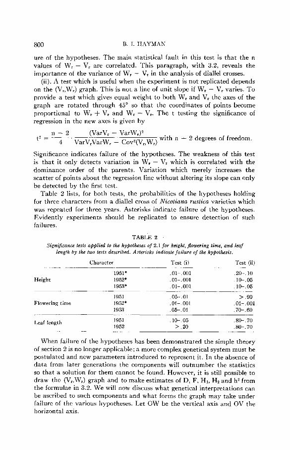
ure of the hypotheses. The main statistical fault in this test is that the n values of W, - V, are correlated. This paragraph, with 3.2, reveals the importance of the variance of W, - V, in the analysis of diallel crosses.

(ii). A test which is useful when the experiment is not replicated depends on the (V,,W,) graph. This is not a line of unit slope if W, - V, varies. To provide a test which gives equal weight to both W, and V, the axes of the graph are rotated through 45" so that the coordinates of points become proportional to W, + V, and W, - V,. The t testing the significance of regression in the new axes is given by

(VarV, - VarW,12 11 - 2 t 2 = - - - . with n - 2 degrees of freedom. 4 VarV,VarW, - Cov2(V,,W,)

Significance indicates failure of the hypotheses. The weakness of this test is that it only detects variation in W, - V, which is correlated with the dominance order of the parents. Variation which merely increases the scatter of points about the regression line without altering its slope can only be detected by the first test.

Table 2 lists, for both tests, the probabilities of the hypotheses holding for three characters from a diallel cross of Nicotiana rusticu varieties which was repeated for three years. Asterisks indicate failure of the hypotheses. Evidently experiments should be replicated to ensure detection of such failures.

TABLE 2 Significance tests applied to the hypotheses of 2.1 for height, flowering time, and leaf

length by the two tests described. Asterisks indicate failure of the hypothesis.

Character Test ( i ) Test (ii) __ .~ ~- ...- ~

1951* . 0 1- ,001 . 2 G . 10 Height 1952* . 01- . 00 1 . 1 G . 05

1953* .01- ,001 . lo-. 05

1951 .0&. 01 > .90

1953 . o s . 01 .70-. 60

... .

Flowering time 1952* .01-. 001 .Ol - . 001

Leaf length 1951 1952

1G.05 > .20

.8@. 70

. SO-. 70

When failure of the hypotheses has been demonstrated the simple theory of section 2 is no longer applicable; a more complex genetical system must be postulated and new parameters introduced to represent it. In the absence of data from later generations the components will outnumber the statistics so that a solution for them cannot be found. However, it is still possible to draw the (V,.W,) graph and to make estimates of D, F, HI, Hz and h2 from the formulae in 3.2. We will now discuss what genetical interpretations can be ascribed to such components and what forms the graph may take under failure of the various hypotheses. Let OW be the vertical axis and OV the horizontal axis.

THE THEORY AND ANALYSIS OF DIALLEL CROSSES 80 1

4.2. Reciprocal diferences. When reciprocal differences exist, two values of each statistic are obtained from the table, one by using the columns, and the other by using the rows, as arrays. This ambiguity may be removed by replacing all entries in the table by their mean reciprocals. If the differences were independent of genotype then estimates of the genetical components are now correct as long as E contains the variation between reciprocals. If the differences depended on genotype then the genetical components are only averages in some way over maternal effects. 3.3 refers to a test for reciprocal differences.

4.3. Residual heterozygosity i n the parents. A full treatment of diallel crosses between partially inbred material will require a separate paper and only the pertinent results are mentioned here. Firstly, the (V,,W,) graph is a scatter about a line of unit slope, points above the line corresponding to heterozygous parents and points below the line to inbred parents. Secondly, the formulae of 3.2 produce underestimates of H1/D and H2/4H1 and an overestimate of F so that the degree of dominance is underestimated, asymmetry of the gene distribution exaggerated and the proportion of dominants overestimated.

4.4. Correlated gene distributions. When the genes at different loci are uncorrelated Cov(&i,&j) = O(i # j) but in the general case we must take

Cov(B,i,&j) = cij. Then, neglecting E, the formulae of 3.2 give r

r O = Zdi'(1 - w.' 1 ) + Zdidjcij

i , # j E' = 2Zdihiwi(l - Wi2) + 22dihjwjcij

A1 = 2hi2(1 - Wiz) + ZhihjCij(WiWj + cij) f i 2 = Zhiz(l - wiz)>" + Zhihjcij'

fi = 2hi(l - wiz). Taking all wi = 0 for simplicity we get

I3 = Zd? + 2didjcij R = O

A1 = 2hi2 + Zhihjcij' = A2

6 = Zhi Since E' = 0 and A1 = fiz the measures of gene frequency are unaffected

by the correlation. $Il (or 8 2 ) is greater than Zhi2 when the dominance is unidirectional, and slightly less if the hi are randomly distributed in sign and magnitude. The estimate of gene number, fi2/k2, is therefore usually depressed by the occurrence of correlation. (= VOLO) is zero when each parent has the same phenotype, and this occurs if each parent contains a suitable combination of positive and negative genes (dispersion). When genes of like effect are together in each parent (association) most cij > 0 and b is greater than Zdi2. Thus the measure of degree of dominance, fil/O, may be either increased or decreased by the combined effects of correlation on and b but the particular combination of dispersion and unidirectional dominance causes serious inflation and may easily turn partial dominance into apparent overdominance.

802 B. I. HAYMAN

The effect on the (V,,W,) graph is interesting. When the cij are small the values of V, still depict the order of dominance. Further

W, - V, = tZ(di2 - hi2)(1 - wiz) + tZ(didj - hihj&iO,j)cij. , # j

The completely dominant and recessive parents correspond to WD - VD = WR - VR = $Z(di2 - hi2)(1 - wiz) + tE(didj - 1hihjl)cij. This is on the average the minimum value of W, - V, for association and the maximum value for dispersion. Parents with intermediate proportions of dominants and recessives correspond to the maximum and minimum values respectively. Hence with association the (V,,W,) curve is convex upwards and with dispersion convex downwards.

4.5. Non-allelic gene interaction. Like 4.3, this heading provides scope for a separate paper. However, we can mention here that, now that a perfectly general representation of gene effect has been developed (HAYMAN and MATHER 1955), genic interaction presents no insuperable problems and we can give some of the pertinent results. A complementary type of interaction distorts the (V,,W,) graph, inflates h1/n, depresses f i 2 / f 1 2 but has little effect on the estimators of gene frequency. A duplicate type of interaction depresses f2/fiz, increases the apparent proportion of dominants but leaves fil/D and fi2/4fi1 and the (V,,W,) graph almost unaltered.

4.6. Scaling. Interaction between genes at non-homologous loci in a single cross may often be eliminated by a suitable change of the scale of measurement, but when interaction has been shown to be present in a diallel cross i t may well be impossible to find one scale on which every individual cross exhibits no interaction. This can, nevertheless, be accomplished when a trend exists between W, - V, on the one hand and both the corresponding parental and array mean values, yr and y,, on the other hand. The method is given by WRIGHT (1.c.).

4.7. Multiple allelism. In the absence of segregation this is equivalent to polygenic biallelism exhibiting genic interaction and distributional correlation as illustrated here. A gene with four alleles forms four homozygotes and is thus equivalent to two genes with two alleles each. There are 9 independent comparisons between ten genotypes, whether derived from the four multiple alleles of one gene, or from two biallelic genes. However, whereas in the first case these comparisons correspond to additive and dominance effects, in the second case only 4 of the comparisons have this property, the others corresponding one to position effect and 4 to genic interaction. Any set of 2p multiple alleles is equivalent in a like manner to p pairs of alleles. A set of q (# 2.) multiple alleles requires p pairs of alleles to represent i t , where 2p-' < q < 2p, but there must also be some genic correlation to reduce the number of homozygotes to q. Evidently the effects of multiple allelism can be extremely complicated.

4.8. When there is no true dominance (all hi = 0) the extended discussion of the previous five sub-sections may be reduced to the simple state- ment that any failure of the hypotheses which can be detected in the (Vr,Wr) graph causes the components estimated by the formulae of 3.2 to

T H E THEORY AND ANALYSIS OF DIALLEL CROSSES 803

exhibit spurious dominance. This follows directly from the concept of the limiting parabola in the (V,,W,) diagram. When there is no dominance all the points should coincide a t (tD,+D) on the limiting parabola. Any failure of the hypotheses which scatters the points (V,,W,) causes their mean (V~L~,WOLO~) to lie inside and not on the limiting parabola. Therefore, from

4.9. Analysis when the hypotheses fail . The approach to the problem of a diallel table exhibiting genic interaction (or indeed any failure of the hypotheses) has been to show how the (V,,W,) graph is affected. This is all that can be done with data from one generation because rescaling (4.6) is not possible if the scale has already been fixed to minimise genotype-environment interaction (3.1). Certainly no exact analysis can be undertaken while the genetical system fails to satisfy the hypotheses of section 2.

The way to further progress is to find some sub-table of the diallel table which does satisfy all the hypotheses and from which valid conclusions may be drawn as to the degree of dominance, asymmetry of gene distribution, etc., in the corresponding sub-group of non-interacting lines. Interacting lines usually have extreme values of W, - V,, i.e. lie well off the line of unit slope through (V~L~,WOLO~). A surer method of discovering which line to eliminate is to remove the measurements on the offspring of each line in turn and to test for heterogeneity of W, - VI in each of the resulting (n - 1) X (n - 1) diallel tables. If any of these heterogeneities is not significant then, as far as this test is concerned, the corresponding sub-table satisfies the hypotheses and the lines remaining in it may be analysed as in sections 2 and 3.

If the interaction is still significant whichever line is removed, the next step is to remove every possible pair of lines in turn and test the remaining sub-tables for heterogeneity of W, - VI, then, if necessary, all triples of lines, etc., until a diallel table satisfying the hypotheses is obtained. In practice, if the removal of no single line can eliminate the interaction, i t is usually sufficient, and far less laborious, instead of removing every possible pair of lines, to remove that line whose omission minimises the heterogeneity and then to remove each of the remaining lines in turn.

When only two values of W, - V, (for r = s and t) show failure of the hypotheses by deviating markedly from the common value of the others, the cause may be interaction in the single cross 8. X et. This is the case when it is possible to adjust the value of this phenotype to make W, - V. and Wt - Vt revert to the common value of the other W, - VI. Theoreti- cally this should be done by minimising the heterogeneity of W, - VI but in practice a missing plot fit based on the analysis of variance of the diallel table (3.3) seems to be good enough and is simpler. If yt. and yst are fitted values then

(n -

2.6, EIi > 0.

- 3>(Y*t + Yt,) = (n - l)(ye. + y.. + Yt. + Y.t - 2ye - 2yt) - 2y.. + 2y.

and (n - 2)(ySt - yt,) = ys. - y.. - yt. + y.t where the sums ys., etc.,

804 B. I. HAYMAN

exclude the missing values. If this adjustment eliminates the interaction the whole table may be analysed without having to omit all the progeny either of Bs or of et.

This procedure of selecting certain lines which conform to the hypotheses is open to the criticism that some sub-group of lines is likely to do so merely through sampling variation. Replication of the experiment in time and space is necessary to validate such selection.

5. SUMMARY OF THE METHOD OF ANALYSIS

(i). Test the variances within families of parents and Fl’s for genotype- environment interaction. This should lie within one of the categories in 3.1 for further analysis to be possible.

(ii). Form the diallel table of reciprocal means, compute V, and W, (r = 1, . . . n) and test W, - V, for heterogeneity (4.1). If this is significant, plot W, - V, against 7, to decide if rescaling would be useful (4.6) and, if this fails, determine the interacting lines or crosses by inspection or otherwise and remove or adjust them (4.9).

(iii). When a diallel table with uniform W, - V, has been obtained analyse its variance to find the significance of some of the genetical components of variation and to provide the estimate of E (3 .3) .

(iv). From V~LO, WOLOI, V l ~ l , VOLI, (mL1 - mL,J2 and the estimate of E compute I3, p, A,, A, and fi2 and find their standard errors (3 .2) .

8, A? (40A,)* + E’ (v). Evaluate and interpret - (2.6), -- (2.5), (4nA,)+ - f; (2.6), and B 4fi1

ii. - (2 .8) when the relevant components are significant. A?

(vi). Note the order of dominance of the parents (3 .2) . Find the correlation between W, + V, and y, and, if i t is significant, predict the limits of selection (2.9).

A quicker and more superficial analysis would omit the analysis of variance of the diallel table and estimate E from differences between reciprocals.

6. NUMERICAL EXAMPLE

6.1. The data used to illustrate the analysis of a diallel table were kindly supplied by D R . JINKS. They are the flowering times, in days from a date in 1952. of Nicotiana rustica plants from a diallel cross of eight inbred varieties. These plants were grown in two blocks each containing 64 plots; each cross or self was represented by 10 progeny, grown in two plots of 5, with one plot in each block. Table 3 contains the mean flowering times per plot of the progeny. The variances within plots do vary significantly, but in the manner described in 3.l(ii) so that it is legitimate to use an average value for E.

6.2. Table 3 also contains the variances, V, of arrays and the covariances, W,. between the arrays and the parental array, calculated for each block from the diallel table of mean reciprocals. W, - V, is reasonably constant except for r = 1 and 3 ; the table shows exceptional and consistent heterosis

THE THEORY AND ANALYSIS OF DIALLEL CROSSES

TABLE 3

Mean $owering time per plot of the progeny of a diallel cross of eighl varieties.

805

1 2 3 4

C? 5 6 7 8

22.8 14.4 27.2 17.2 18.3 16.2 18.6 16.4 15.4 17.2 14.8 18.6 15.2 17.0 14.4 10.8 31.8 21.0 24.8 24.6 19.2 29.8 12.8 13.0 16.2 11.4 16.8 18.4 12.4 16.8 12.6 9 .6 14.6 12.2 15.2 15.2 15.2 18.0 10.4 13.4 20.2 14.2 18.6 22.2 14.3 20.2 9 .0 11.8 14.0 12.2 13.6 13.8 15.6 15.6 11.4 13.0 15.2 10.0 17.0 20.8 20.0 17.0 13.0 14.0

W,

18.29 7.44

23.17 10.37 4.41

15.38 3.72 2.67

1 2 3 4

d 5 6 7 8

Block I1

1

24.2 16.5 30.4 17.8 18.8 23.4 16.6 17.2

0 2 3 4 5 6 7 8 W,

16.2 30.8 27.0 18.8 14.6 18.6 23.0 21.2 25.4 13.0 16.3 18.0 13.8 15.4 13.8 14.0 14.8 17.0 9 . 2 16.2 14.4

11.6 18.2 20.8

20.2 15.3 20.0 14.2 L5.2 17.3 15.6 17.4

16.8 14.4 16.0 15.2 11.8 13.2 28.4 14.2 14.4 14.8 12.2 11.2 16.0 12.2 20.0 22.6 10.2 12.8 11.0 10.6 9 .8 12.6 9 . 8 15.8

14.02 7.18

17.91 11.10 5.73

16.57 4.84 4.04

x T wr - v, v r

24.46 5.55

30.59 7.48 2.53

14.10 1.96 3.76

vr 25.39 6.61

22.84 10.19 4.82

18.35 4.79 8.33

-6.18 1.89

-7.42 2.89 1.88 1.28 1.76

-1.08

wr - v r

-11.37 0.56

-4.93 0.91 0.91

-1.79 0.05

-4.29

in the progeny of the corresponding crosses. The tests of 4.1 confirm heterogeneity of W, - V,.

(i). The analysis of the variance of W, - V, is

Mean square Df P Lines 31.67 '7 .01-.001 Blocks 13.98 1 .05-.01 Error 2.46 7

(ii). In the test of the deviation of the slope of the (V,,W,) line from unity, tI4 = 4.068 and P = .01-.001, which is highly significant.

The significant variation of W, - V, from line to line means that these diallel tables do not satisfy the hypotheses of section 2. The graph of W, - V, against , reveals no trend so that a change of scale is not suggested. The source of the trouble is probably complementary gene action in the cross el X e3, and an adjustment of the plot means of the progeny of this cross should make the diallel cross conform to the hypotheses.

The formulae of 4.9 provide estimates of the plot means in the diallel table of means over the two blocks. The estimate of the difference between any two corresponding plot means in the two blocks = (BI total - BII total)/(n2 - 2) which minimises the block interaction sum of squares in the analysis of variance of two diallel tables. (The totals, as in 4.9, exclude the means of the progeny of el x e,). The estimated plot means are

806

0

B. I. HAYMAN

I I I I I I

5 '0 v, 15 2 0 25 3 0

\

Block 9 1 x 8 3 P 3 x 8 1

I 23.3 19.2 I1 23.6 19.6

which are about two-thirds of the observed values. The other new entries in Table 3 are

Block W1 v1 w1 -v1 w3 v3 w3 - v3 I 10.27 7.82 2.45 17.51 17.44 1.37 I1 10.29 9.94 0.34 10.33 6.44 3.89

The tests now show W, - V, to be uniform (i). In the analysis of variance of W, - V, the probabilities of both line

(ii). The slope of the (V,,W,) line does not differ significantly from unity

6,3. We are now free to analyse the variance of the diallel tables and to

and block mean squares are .20-.lo.

(P > .SO).


find the components of variation, remembering, of course, that our results provide no information about the cross X e,. Figure 2 depicts the points (V,,W,), the limiting parabola W,Z = Vo~oV,, and the line of unit slope through the adjusted mean point (V~LI,WOLOI). The unadjusted points lie well off this line.

The analysis of variance is derived from the adjusted table 3 in the way described by HAYMAN (I.c.). Table 4 contains the significance levels of the

TABLE 4 Signijicance leuels of the components of variance derived from the data in tuble 3.

Item Probability (a) D - F + HI - Hz < .001 (bJ hz < ,001 (bz) HI - Hz > .20 (bs) < ,001 (b) Hz < .001 (c) Reciprocal < .001 (d) differences <.001 (B) Blocks > .20

components. The significance of (b) shows that dominance is present while (bl) shows that it is largely unidirectional. From the sign of h we see that the progeny mean is less than the parental mean so that this dominance is in the direction of early flowering time. Asymmetry is not significant (bz) at loci exhibiting dominance. This also implies that (a) detects purely additive variation and this is highly significant. The significant differences between reciprocal families are an unfortunate systematic effect due to faulty lay-out of seed-boxes in the greenhouse so that the use of mean reciprocals in all other computations is justified. The overall block difference is not significant. The block interaction mean square, which is the estimate of E, is 3.37.

Block VOLO WoLol VlLl VOLI (mu - mLd2

6.4. The values of the statistics of 3.2 are

I 20.33 8.97 7.58 4.20 3.63 I1 19.60 8.76 8.68 5.13 3.41

and the mean estimates of the components of variation with their standard errors are

I3 F AI A2 f i 2 B D - f i 1

16.59 - 0.59 7.76 7.11 12.60 3.37 8.83 f 1 . 7 9 f4.24 f4.12 f 3 . 5 9 f2.40 f 0 . 6 0 f 3 . 5 4

The sum of the squares of deviations of observed from expected values of VOL', VILI, V, and W, (r = 1, . . . n) is 142.84. The two diallel tables supply 37 statistics, and 12 constants are fitted to them, leaving 25 degrees of freedom for error. Hence the mean squared deviation is 5.71. Now, from the top left corner of the matrix in table 1, Varf) = $(n + l)s2/n, the factor of 4 allowing for the use in the estimation of means of statistics from two blocks. Since n = 8 and s2 = 5.71, VarG = 3.21. Similarly, from the

SOS B. I. HAYMAN

next term down the leading diagonal of the matrix, Varp = X 6.28 x 5.71 = 17.94, etc. The square roots of these variances give the standard errors above. Their large values are due to the variations in V3 and W3 between blocks which suggest that this variety is unstable to environmental variations. Apparently fi, and k2 are not quite significant but the more reliable analysis of variance in 6.3 shows that k, is significant. Here D - AI is just significantly different from zero; it is highly so if we use the zimple formula for Var (0 - k,) a t the end of 3.2 which gives a standard error of 1.96 for 0 - Al. Evidently dominance is present but it is definitely not complete dominance.

6.5. (Hl/fi)* = 0.6s is an estimate of the mean degree of dominance over all loci. In figure 2, AB/OB estimates Hl/D without allowing for E. If the formulae of 3.2 are applied to the original diallel tables (i.e. without adjust- ing the cross el x e,) then (A1/D)* = 1.02. This illustrates the extent to which nonallelic genic interaction can inflate this estimate of the degree of dominance and emphasises the importance of the preliminary survey with the (V,,W,) graph.

The estimate of uv is fi2/&, = 0.23 agreeing with the result in the analysis of variance (6.3) that H, is not significantly different from H1.

{ (40fi,)* + PI/{ (4hH1)$ - = 0.95 which is near enough to unity, implying equality between the numbers of dominant and recessive alleles in the parents. This is, of course, a necessary consequence of the foregoing result that ui = v, = 3.

h 2 / f i 2 = 1.77 so that a t least two of the genes controlling flowering time exhibit some degree of dominance.

6.6. The order of dominance of the parents, determined by W, + V,, is 75821436 and the order of flowering time is 78524631, parent 7 being the earliest and carrying the most dominants. The correlation between yr and W, + V, is 0.80 corroborating our result above (6.3) that early flowering is partially dominant.

6.7. This example has been worked in detail more to illustrate our methods and some of the difficulties which arise than to present a set of results conforming closely to our theories. Measurements of height and leaf length from the same plants were more consistent than flowering time over the two blocks and showed less or no reciprocal differences and little genotype- environment interaction. Further, while height exhibited genic interaction, leaf length satisfied our hypotheses completely.

SUMMARY

Experiments with diallel crosses provide a powerful method of investigating polygenic systems. The theory of a diallel cross between homozygous lines is discussed in terms of components of variation similar to MATHER’S (I.c.) D and H components. Assuming a simple underlying genetical system, we show that the various statistics obtained from measurements on the progeny provide estimates of the overall degree of dominance, of the rela-


tive dominance properties of the parents, and of the symmetry or otherwise of the gene distribution in the lines. The dominance relations are exhibited graphically. The effects of complications such as genic interaction are also considered. A genetic algebra is used to simplify the mathematical computations. The final sections are a summary of the method of analysis and a worked example.

LITERATURE CITED

HAYMAN, B. I., 1954 HAYMAN, B. I. and K. MATHER, 1955

HULL, F. H., 1945

The analysis of variance of diallel crosses. Biometrics 10: 235-244. The description of genic interaction in continuous

Regression analyses of yields of hybrid corn and inbred parent lines.

Overdominance and recurrent selection. Heterosis, chap. 28, Iowa State College

The analysis of heritable variation in a diallel cross of Nicotiana rustica

The analysis of diallel crosses. Maize Genetics News

variation. Biometrics (in press).

Maize Genetics News Letter 19: 21-27. 1952 Press, Ames, Iowa.

JINKS, J. L., 1954 varieties. Genetics 39: 767-788.

JINKS, J. L. and B. I. HAYMAN, 1953 Letter 27: 48-54.

MATHER, K., 1949 MATHER, K. and A. VINES, 1962

WRIGHT, S., 1952

Biometrical Genetics. London, Methuen and Co. The inheritance of height and flowering time in a cross

The genetics of quantitative variability. Quantitative Inheritance, 5-41, of Nicotiana rustica. Quant-itative Inheritance, 49-80, H.M.S.O., London.

H.M.S.O., London.

b. · the theory and analysis of diallel crosses* b. i. hayman a .r. c. unit of biometrical...

Documents