b-737 linear autoland simulink model - old dominion …mln/ltrs-pdfs/nasa-2004-cr213021.pdf ·...
TRANSCRIPT

May 2004
NASA/CR-2004-213021
B-737 Linear Autoland Simulink Model
Edward F. Hogge
Lockheed Martin Corporation, Hampton, Virginia
The NASA STI Program Office . . . in Profile
Since its founding, NASA has been dedicated to the
advancement of aeronautics and space science. The
NASA Scientific and Technical Information (STI)
Program Office plays a key part in helping NASA
maintain this important role.
The NASA STI Program Office is operated by
Langley Research Center, the lead center for NASA’s
scientific and technical information. The NASA STI
Program Office provides access to the NASA STI
Database, the largest collection of aeronautical and
space science STI in the world. The Program Office is
also NASA’s institutional mechanism for
disseminating the results of its research and
development activities. These results are published by
NASA in the NASA STI Report Series, which
includes the following report types:
TECHNICAL PUBLICATION. Reports of
completed research or a major significant phase
of research that present the results of NASA
programs and include extensive data or
theoretical analysis. Includes compilations of
significant scientific and technical data and
information deemed to be of continuing
reference value. NASA counterpart of peer-
reviewed formal professional papers, but having
less stringent limitations on manuscript length
and extent of graphic presentations.
TECHNICAL MEMORANDUM. Scientific
and technical findings that are preliminary or of
specialized interest, e.g., quick release reports,
working papers, and bibliographies that contain
minimal annotation. Does not contain extensive
analysis.
CONTRACTOR REPORT. Scientific and
technical findings by NASA-sponsored
contractors and grantees.
CONFERENCE PUBLICATION. Collected
papers from scientific and technical
conferences, symposia, seminars, or other
meetings sponsored or co-sponsored by NASA.
SPECIAL PUBLICATION. Scientific,
technical, or historical information from NASA
programs, projects, and missions, often
concerned with subjects having substantial
public interest.
TECHNICAL TRANSLATION. English-
language translations of foreign scientific and
technical material pertinent to NASA’s mission.
Specialized services that complement the STI
Program Office’s diverse offerings include creating
custom thesauri, building customized databases,
organizing and publishing research results ... even
providing videos.
For more information about the NASA STI Program
Office, see the following:
Access the NASA STI Program Home Page at
http://www.sti.nasa.gov
E-mail your question via the Internet to
Fax your question to the NASA STI Help Desk
at (301) 621-0134
Phone the NASA STI Help Desk at
(301) 621-0390
Write to:
NASA STI Help Desk
NASA Center for AeroSpace Information
7121 Standard Drive
Hanover, MD 21076-1320

National Aeronautics and
Space Administration
Langley Research Center Prepared for Langley Research Center
Hampton, Virginia 23681-2199 under Contract NAS1-00135
May 2004
NASA/CR-2004-213021
B-737 Linear Autoland Simulink Model
Edward F. Hogge
Lockheed Martin Corporation, Hampton, Virginia

Available from:
NASA Center for AeroSpace Information (CASI) National Technical Information Service (NTIS)
7121 Standard Drive 5285 Port Royal Road
Hanover, MD 21076-1320 Springfield, VA 22161-2171
(301) 621-0390 (703) 605-6000
Acknowledgments
I would like to thank Dr. Alan White for his assistance in the description of the Dryden
gust model mathematics and the random number generator repair. I would like to thank
Arlene Guenther of Unisys for help with understanding and adapting the original
FORTRAN Airlabs model and the document that this is adapted from. Also, thanks to
Dr. L. Keith Barker for his help with reference frames and general mathematical analysis
suggestions.
The use of trademarks or names of manufacturers in the report is for accurate reporting and does not
constitute an official endorsement, either expressed or implied, of such products or manufacturers by the
National Aeronautics and Space Administration.
1
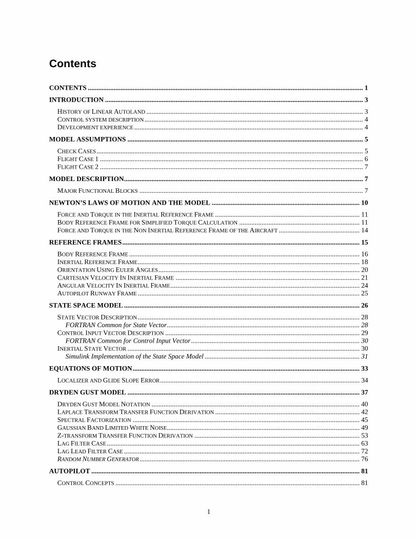
Contents
CONTENTS ................................................................................................................................................................ 1
INTRODUCTION ...................................................................................................................................................... 3
HISTORY OF LINEAR AUTOLAND .............................................................................................................................. 3 CONTROL SYSTEM DESCRIPTION ............................................................................................................................... 4 DEVELOPMENT EXPERIENCE ..................................................................................................................................... 4
MODEL ASSUMPTIONS ......................................................................................................................................... 5
CHECK CASES........................................................................................................................................................... 5 FLIGHT CASE 1 ......................................................................................................................................................... 6 FLIGHT CASE 2 ......................................................................................................................................................... 7
MODEL DESCRIPTION........................................................................................................................................... 7
MAJOR FUNCTIONAL BLOCKS .................................................................................................................................. 7
NEWTON’S LAWS OF MOTION AND THE MODEL ...................................................................................... 10
FORCE AND TORQUE IN THE INERTIAL REFERENCE FRAME .................................................................................... 11 BODY REFERENCE FRAME FOR SIMPLIFIED TORQUE CALCULATION ...................................................................... 11 FORCE AND TORQUE IN THE NON INERTIAL REFERENCE FRAME OF THE AIRCRAFT ............................................... 14
REFERENCE FRAMES.......................................................................................................................................... 15
BODY REFERENCE FRAME ...................................................................................................................................... 16 INERTIAL REFERENCE FRAME................................................................................................................................. 18 ORIENTATION USING EULER ANGLES..................................................................................................................... 20 CARTESIAN VELOCITY IN INERTIAL FRAME ........................................................................................................... 21 ANGULAR VELOCITY IN INERTIAL FRAME.............................................................................................................. 24 AUTOPILOT RUNWAY FRAME ................................................................................................................................. 25
STATE SPACE MODEL ......................................................................................................................................... 26
STATE VECTOR DESCRIPTION ................................................................................................................................. 28 FORTRAN Common for State Vector................................................................................................................ 28
CONTROL INPUT VECTOR DESCRIPTION ................................................................................................................. 29 FORTRAN Common for Control Input Vector.................................................................................................. 30
INERTIAL STATE VECTOR ....................................................................................................................................... 30 Simulink Implementation of the State Space Model .......................................................................................... 31
EQUATIONS OF MOTION.................................................................................................................................... 33
LOCALIZER AND GLIDE SLOPE ERROR.................................................................................................................... 34
DRYDEN GUST MODEL ....................................................................................................................................... 37
DRYDEN GUST MODEL NOTATION ......................................................................................................................... 40 LAPLACE TRANSFORM TRANSFER FUNCTION DERIVATION .................................................................................... 42 SPECTRAL FACTORIZATION .................................................................................................................................... 45 GAUSSIAN BAND LIMITED WHITE NOISE................................................................................................................ 49 Z-TRANSFORM TRANSFER FUNCTION DERIVATION ................................................................................................ 53 LAG FILTER CASE................................................................................................................................................... 63 LAG LEAD FILTER CASE ......................................................................................................................................... 72 RANDOM NUMBER GENERATOR ................................................................................................................................ 76
AUTOPILOT ............................................................................................................................................................ 81
CONTROL CONCEPTS .............................................................................................................................................. 81
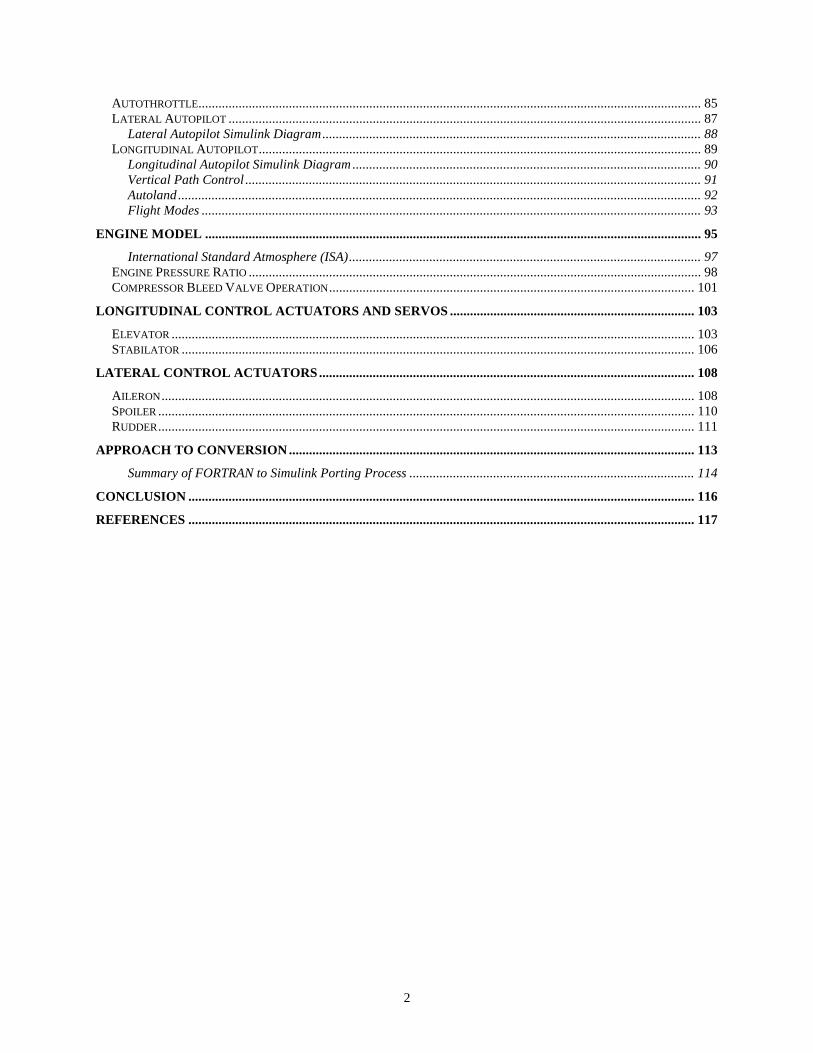
2
AUTOTHROTTLE...................................................................................................................................................... 85 LATERAL AUTOPILOT ............................................................................................................................................. 87
Lateral Autopilot Simulink Diagram................................................................................................................. 88 LONGITUDINAL AUTOPILOT.................................................................................................................................... 89
Longitudinal Autopilot Simulink Diagram ........................................................................................................ 90 Vertical Path Control ........................................................................................................................................ 91 Autoland ............................................................................................................................................................ 92 Flight Modes ..................................................................................................................................................... 93
ENGINE MODEL .................................................................................................................................................... 95
International Standard Atmosphere (ISA)......................................................................................................... 97 ENGINE PRESSURE RATIO ....................................................................................................................................... 98 COMPRESSOR BLEED VALVE OPERATION............................................................................................................. 101
LONGITUDINAL CONTROL ACTUATORS AND SERVOS ......................................................................... 103
ELEVATOR ............................................................................................................................................................ 103 STABILATOR ......................................................................................................................................................... 106
LATERAL CONTROL ACTUATORS................................................................................................................ 108
AILERON............................................................................................................................................................... 108 SPOILER ................................................................................................................................................................ 110 RUDDER................................................................................................................................................................ 111
APPROACH TO CONVERSION ......................................................................................................................... 113
Summary of FORTRAN to Simulink Porting Process ..................................................................................... 114
CONCLUSION ....................................................................................................................................................... 116
REFERENCES ....................................................................................................................................................... 117
3
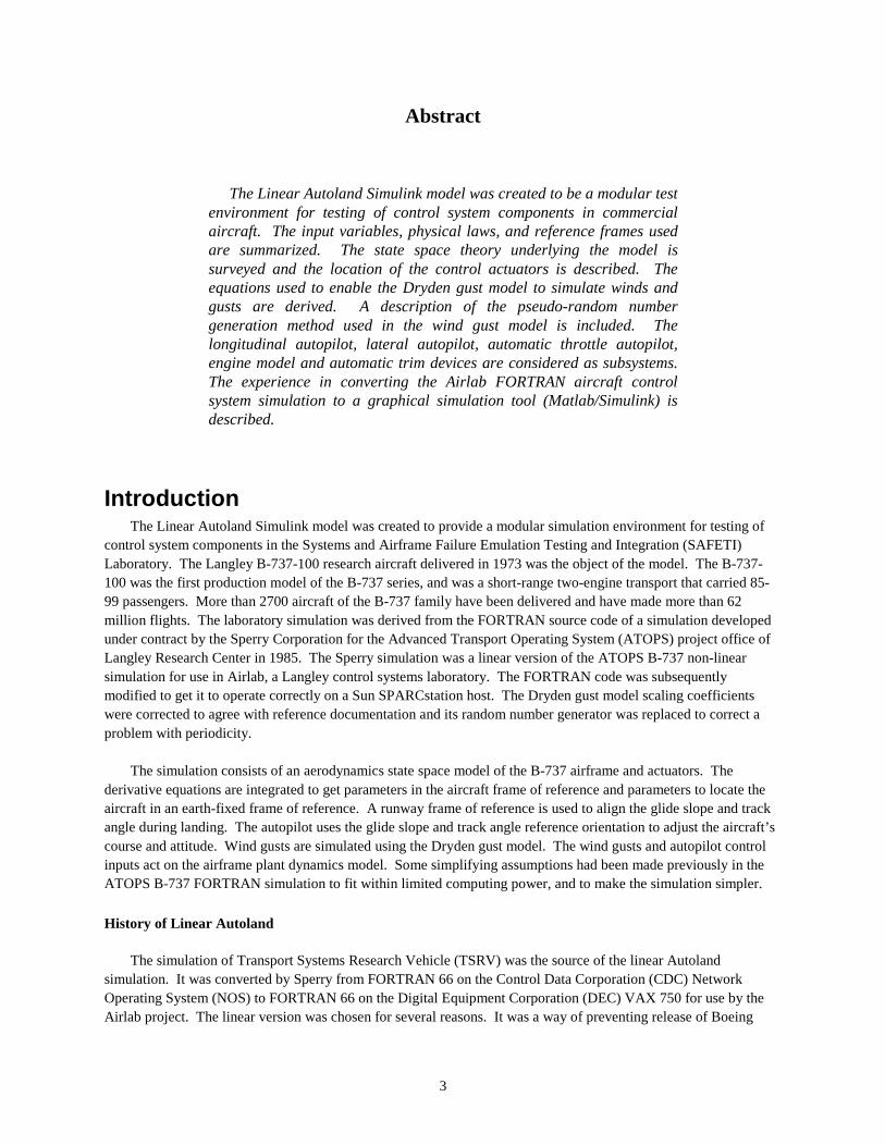
Abstract
The Linear Autoland Simulink model was created to be a modular test environment for testing of control system components in commercial aircraft. The input variables, physical laws, and reference frames used are summarized. The state space theory underlying the model is surveyed and the location of the control actuators is described. The equations used to enable the Dryden gust model to simulate winds and gusts are derived. A description of the pseudo-random number generation method used in the wind gust model is included. The longitudinal autopilot, lateral autopilot, automatic throttle autopilot, engine model and automatic trim devices are considered as subsystems. The experience in converting the Airlab FORTRAN aircraft control system simulation to a graphical simulation tool (Matlab/Simulink) is described.
Introduction
The Linear Autoland Simulink model was created to provide a modular simulation environment for testing of control system components in the Systems and Airframe Failure Emulation Testing and Integration (SAFETI) Laboratory. The Langley B-737-100 research aircraft delivered in 1973 was the object of the model. The B-737-100 was the first production model of the B-737 series, and was a short-range two-engine transport that carried 85-99 passengers. More than 2700 aircraft of the B-737 family have been delivered and have made more than 62 million flights. The laboratory simulation was derived from the FORTRAN source code of a simulation developed under contract by the Sperry Corporation for the Advanced Transport Operating System (ATOPS) project office of Langley Research Center in 1985. The Sperry simulation was a linear version of the ATOPS B-737 non-linear simulation for use in Airlab, a Langley control systems laboratory. The FORTRAN code was subsequently modified to get it to operate correctly on a Sun SPARCstation host. The Dryden gust model scaling coefficients were corrected to agree with reference documentation and its random number generator was replaced to correct a problem with periodicity.
The simulation consists of an aerodynamics state space model of the B-737 airframe and actuators. The derivative equations are integrated to get parameters in the aircraft frame of reference and parameters to locate the aircraft in an earth-fixed frame of reference. A runway frame of reference is used to align the glide slope and track angle during landing. The autopilot uses the glide slope and track angle reference orientation to adjust the aircraft’s course and attitude. Wind gusts are simulated using the Dryden gust model. The wind gusts and autopilot control inputs act on the airframe plant dynamics model. Some simplifying assumptions had been made previously in the ATOPS B-737 FORTRAN simulation to fit within limited computing power, and to make the simulation simpler.
History of Linear Autoland
The simulation of Transport Systems Research Vehicle (TSRV) was the source of the linear Autoland simulation. It was converted by Sperry from FORTRAN 66 on the Control Data Corporation (CDC) Network Operating System (NOS) to FORTRAN 66 on the Digital Equipment Corporation (DEC) VAX 750 for use by the Airlab project. The linear version was chosen for several reasons. It was a way of preventing release of Boeing
4
proprietary aerodynamic data present in the full non-linear version. The target host VAX 750 was not fast enough to run the full non-linear equations. Also, too much programming labor would have been required to convert the non-linear aerodynamic data in CDC packed binary format to VAX format. The linear VAX version was good enough to satisfy the research requirements of Airlab.
Lockheed Martin was contracted to port the Airlab linear Autoland version from the VAX environment to the Sun Microsystems Unix workstation FORTRAN 77 environment for the SAFETI Laboratory. Subroutine calling sequences and parameter lists were aligned to correct repeatability problems. The Dryden gust model was repaired by changing filter coefficients to agree with published literature and by replacing a defective random number generator. A gust response of an order of magnitude larger was the result in the reference flight case 1, and was in agreement with the expectations of a NASA control engineer familiar with the Boeing 737 response to control inputs.
Control system description
The control system consists of three major sections, the lateral autopilot, the longitudinal autopilot, and the automatic throttle. The lateral autopilot uses the spoilers, ailerons, and rudder to control the flight path left to right according to a heading set point. The longitudinal autopilot uses the elevator and stabilator to control the glide slope angle up and down according to a glide slope set point. The automatic throttle uses a target air speed to adjust the engine throttle in order to maintain a constant air speed. During the automatic landing phase of the flight, the lateral and longitudinal set points are replaced by track and glide slope error derived from radio transmitters at the destination runway. The error in heading is provided by the difference between the orientation of the aircraft path and a line to the localizer radio transmitter. The error in glide slope is provided by the difference between the flight path and a line to the glide slope transmitter. The automatic throttle maintains a constant airspeed. This situation continues until the final phase of the landing.
Development experience
Lockheed Martin was contracted to port the FORTRAN Linear Autoland model to Matlab/Simulink. Matlab and Simulink are software tools for engineering analysis produced by The MathWorks Inc. They are commonly used by universities and engineering companies for control system simulation and development. The FORTRAN model was converted to Simulink according to a black-box procedure. The unchanged FORTRAN code was called from Simulink using Matlab dynamically linked subroutine (FORTRAN MEX) blocks. The FORTRAN modules used were those which modeled the aerodynamics and equations of motion. An open-loop configuration to simulate a straight, level flight condition was tested and explored. Once that configuration was operating repeatably, time histories of control parameters were substituted for the straight, level flight condition as input to the model. Corrections were made until the model parameters roughly matched the reference FORTRAN simulation runs. Next, subsystems of the FORTRAN model were replaced step-wise by Simulink blocks. When the Simulink blocks had completely replaced the FORTRAN subroutines, work began on the autopilot. A Simulink version of each autopilot subsystem was substituted for the corresponding time history input. This closed the loop in the simulation. Sources of error were isolated by detailed comparison of model time histories with the FORTRAN reference runs.
5
Model Assumptions The Sperry Linear 737 Autoland Simulation for Airlabs [Ref. 9] made simplifying assumptions to protect
Boeing proprietary aerodynamic data, and to make analysis easier. Because the Airlab version was constrained by limited computer power, little attention was given to conversion of the Dryden gust model from the CDC NOS FORTRAN 66 implementation to the Airlab version because Airlab had few requirements for testing gust response. Here is a summary of the assumptions present in the Airlab’s FORTRAN simulation and carried over to the B-737 Linear Autoland Simulink model.
• Linearized State Space Model
• No Boeing Proprietary Data
• Similar Dynamics and Control (A and B) Matrices for Flight Cases 1 and 2
• One Engine Instead of Two
• (The thrust is half that of the actual airplane. The state space model works as if the other engine were there. The throttle setting is the same as the actual airplane.)
• Flight Ends After Flare But Before Roll Out
• Constant Flaps, Set At 40 deg
• Center of Mass (Gravity) Set At 0.2 Fraction of Length of Fuselage or At 20% Mean Aerodynamic Chord (MAC)
• Gross Weight 85000 lbs
• Length 94 ft
• Wingspan 93 ft
• Tail Height 37 ft
• Langley AFB Runway 8 Approached From the West
Check Cases
In order to prevent the introduction of errors into the simulation during the software conversion, time histories of important parameters were generated. The only information available from the original CDC NOS computer runs was strip chart time histories of flight case 2 engineering parameters. These strip charts were used to diagnose problems introduced into the FORTRAN simulation at the time of the conversion to run on the Airlab VAX. The software modifications necessary to run on the Sun were checked also. Once a valid and repeatable FORTRAN simulation was achieved on the Sun equipment, reference files of parameter time histories were saved. The FORTRAN source code configuration was maintained using the UNIX SCCS commands. The version described in
6
this document is g134v1.
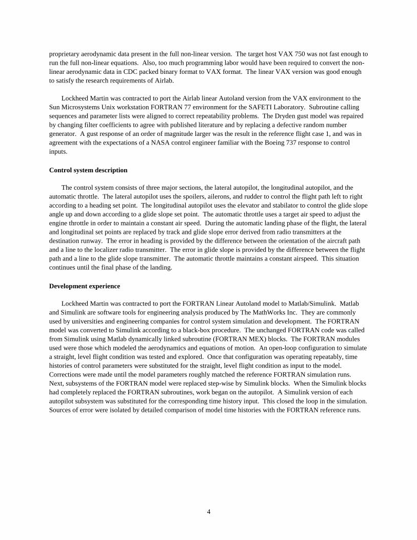
Figures 1 and 2 depict the path of the simulated aircraft for flight cases 1 and 2, respectively, and describe the flight conditions.
Flight Case 1
• Straight in approach, below glide slope along extended center line
• Capture glide slope from below
• Wind from Northeast, 20 knots
Figure 1. Path of simulated aircraft for flight case 1.
There is a sharp pitch change at the beginning of flight case 1. It is a good test to find stability problems with the longitudinal control system. It does not exercise the lateral control system at all.
0
2000
1000
-76.5
-76.4
36.9
37.1
37.0
37.2
-76.6
-76.3
N
Alti
tude
(ft
)
LatitudeLongitude
Wind
20 knots
Runway

7
Flight Case 2
• Turning from base to final approach. Bank to left to capture glide slope, 130 degs. localizer capture followed by glide slope capture
• No wind
Figure 2. Path of simulated aircraft for flight case 2.
The bank to the left tests if the centrifugal and Coriolis forces are accounted for correctly. The lateral control
system is exercised. Interaction of the ailerons with the spoilers is tested as well.
Model Description Major Functional Blocks
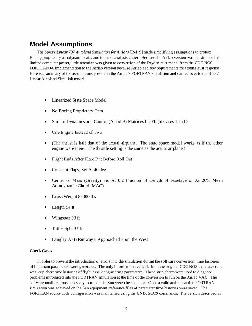
The FORTRAN linear Autoland simulation consists of a series of functional modules. At first glance it seems like it would be easy to separate the modules by function as if they were “black boxes”. The initialization of global memory from file and terminal dialog is managed in the initialization module “a737int”. The equations of motion are mostly located in the module “eqmotn” as is the Dryden gust model. The Autopilot module “a737inp” comes next in the loop after the equations of motion module, and this is counterintuitive. All three autopilot systems, lateral, longitudinal, and thrust control are contained there. The control surface models modify the control parameter inputs of aileron, elevator, thrust, and rudder and drive the state space model contained in the differentiation and integration module “deriv_ab2”. The automatic systems that control the stabilator, engine, and yaw damping of the rudder are part of the “deflect” module and not the autopilot module.
0
2000
1000
-76.5
-76.4
36.9
37.1
37.0
37.2
-76.6
-76.3
N
Alti
tude
(ft
)
LatitudeLongitude
Runway
8
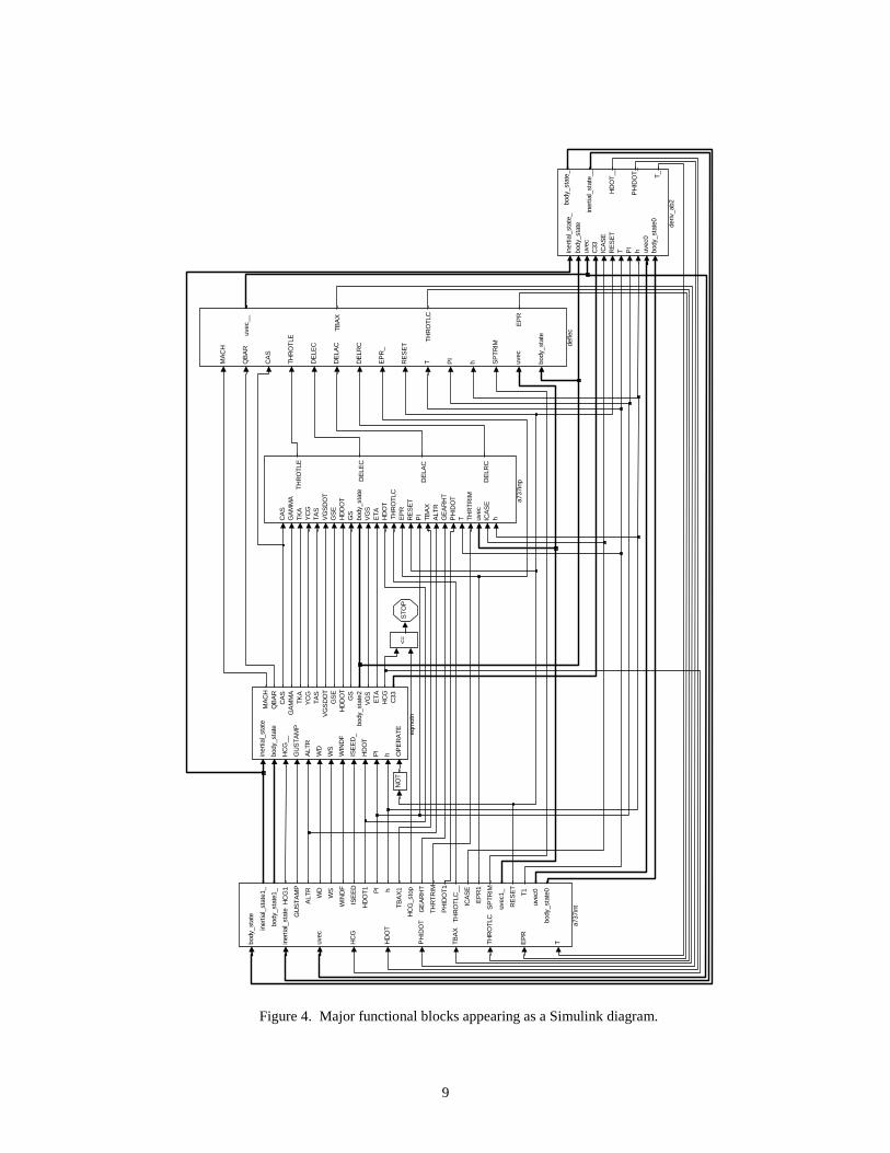
Figure 3. Data flow of the B-737 Autoland Simulation
The modules are coupled through subroutine calling sequences and global memory (FORTRAN common blocks). Data flow is hard to discern due to global memory linkage of subroutines and multiple names for the same global memory location through the use of the FORTRAN “equivalence” statement. The order of execution of the blocks is important because of the modification of the body reference frame velocities and rotations by the inertial reference frame accelerations in the “deriv_ab2” module. First order lag filters and other modules use parameter values from the previous iteration to filter the current parameters.
The Simulink top level diagram is divided up into blocks similar to the FORTRAN model. There are more lines here because this is the actual source code diagram with all the variable linkages. Notice all the modules shown in the previous figure are present.
Initializationand StateMemory
a737int
Equationsof Motion
eqmotn
Autopilot
a737inp
ControlSurfaceModelsdeflec
Differentiationand Integration
deriv_ab2
9
Figure 4. Major functional blocks appearing as a Simulink diagram.
ST
OP
iner
tial_
stat
e
body
_sta
te
HC
G__
GU
ST
AM
P
ALT
R
WD
WS
WIN
DF
ISE
ED
_
HD
OT
PI
h OP
ER
AT
E
MA
CH
QB
AR
CA
SG
AM
MA
TK
AY
CG
TA
SV
GS
DO
TG
SE
HD
DO
TG
Sbo
dy_s
tate
2V
GS
ET
AH
CG
C33
eqm
otn
iner
tial_
stat
e_bo
dy_s
tate
uvec
C33
ICA
SE
RE
SE
TT P
Ih uv
ec0
body
_sta
te0
body
_sta
te_
iner
tial_
stat
e__
HD
OT
__
PH
IDO
T_
T_
deriv
_ab2
MA
CH
QB
AR
CA
S
TH
RO
TLE
DE
LEC
DE
LAC
DE
LRC
EP
R_
RE
SE
T
T PI
h SP
TR
IM
uvec
body
_sta
teuvec
__
TB
AX
TH
RO
TLC
EP
R
defle
c
body
_sta
te
iner
tial_
stat
e
uvec
HC
G
HD
OT
PH
IDO
T
TB
AX
TH
RO
TLC
EP
R
T
iner
tial_
stat
e1_
body
_sta
te1_
HC
G1
GU
ST
AM
P
ALT
R
WD
WS
WIN
DF
ISE
ED
HD
OT
1 PI h
TB
AX
1
HC
G_s
top
GE
AR
HT
TH
RT
RIM
PH
IDO
T1
TH
RO
TLC
__
ICA
SE
EP
R1
SP
TR
IM
uvec
1_
RE
SE
T
T1
uvec
0
body
_sta
te0
a737
int
CA
SG
AM
MA
TK
AY
CG
TA
SV
GS
DO
TG
SE
HD
DO
TG
Sbo
dy_s
tate
VG
SE
TA
HD
OT
TH
RO
TLC
EP
RR
ES
ET
PI
TB
AX
ALT
RG
EA
RH
TP
HID
OT
T TH
RT
RIM
uvec
ICA
SE
h
TH
RO
TLE
DE
LEC
DE
LAC
DE
LRC
a737
inp
<=N
OT

10
Newton’s Laws of Motion and the Model The FORTRAN and Simulink Autoland simulations both are based on the application of Newton’s second law
of motion maF = for force, mass and acceleration. The three Cartesian components of motion come from this. The three rotational components of motion come from application of the rotational motion form of the second law,
α=τ I . Torque replaces force, rotational inertia replaces mass, and rotational acceleration replaces Cartesian acceleration [Ref. 11].
Table 1. Motion Equations, Inertial Reference Frame
Rectilinear Motion
Rotation about a Fixed Axis
Displacement x Angular Displacement θ
Velocity
dt
dxv =
Angular Velocity
dt
dθ=ω
Acceleration
dt
dva =
Angular Acceleration
dt
dω=α
Mass m Rotational Inertia I
Linear Momentum mvp = Angular Momentum ω= Ih
Force maF = Torque α=τ I
dt
dvmF =
dt
dI
ω=τ
dt
dpF =
dt
dh=τ
These six equations can be collected into two vector equations. The mass and acceleration terms can be expressed as derivatives of momentum and angular momentum.
11
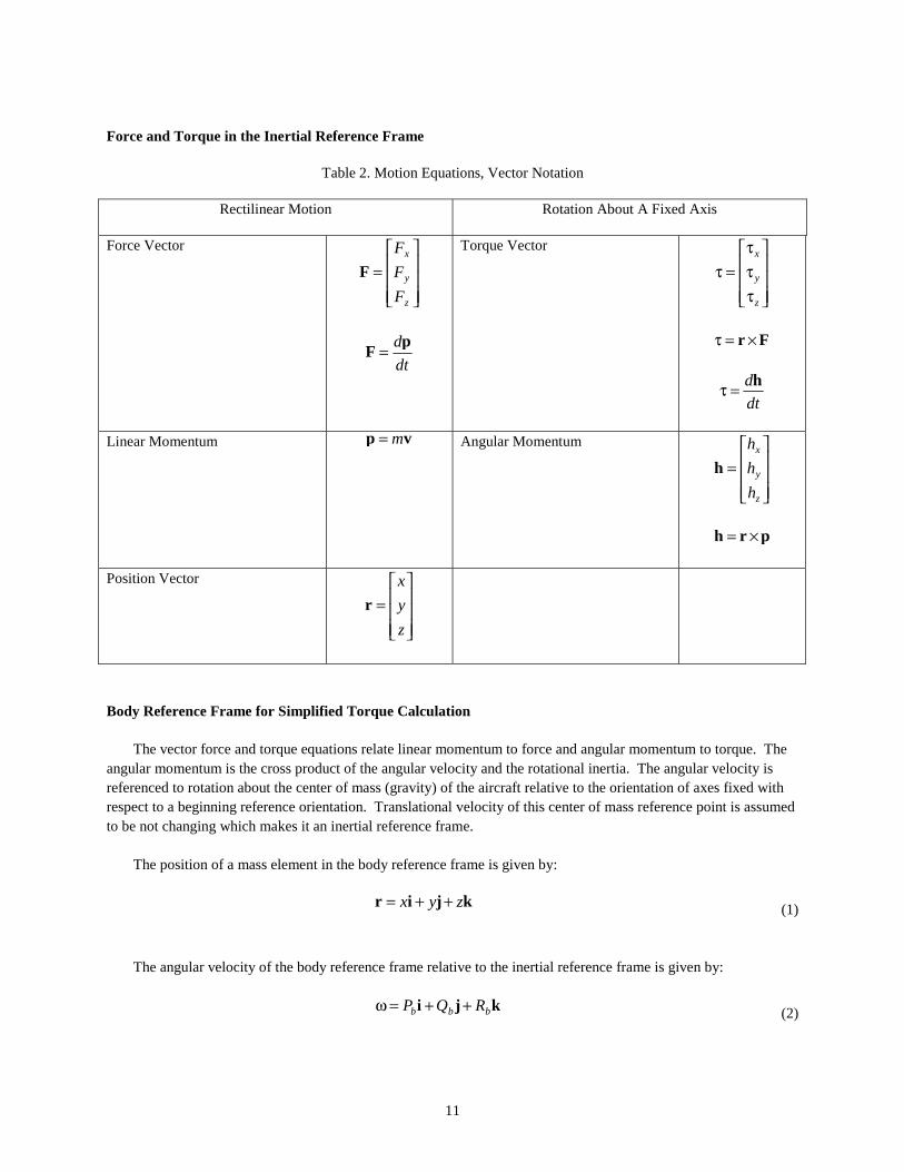
Force and Torque in the Inertial Reference Frame
Table 2. Motion Equations, Vector Notation
Rectilinear Motion
Rotation About A Fixed Axis
Force Vector
=
z
y
x
F
F
F
F
dt
dpF =
Torque Vector
τττ
=τ
z
y
x
Fr ×=τ
dt
dh=τ
Linear Momentum vp m= Angular Momentum
=
z
y
x
h
h
h
h
prh ×=
Position Vector
=
z
y
x
r
Body Reference Frame for Simplified Torque Calculation
The vector force and torque equations relate linear momentum to force and angular momentum to torque. The angular momentum is the cross product of the angular velocity and the rotational inertia. The angular velocity is referenced to rotation about the center of mass (gravity) of the aircraft relative to the orientation of axes fixed with respect to a beginning reference orientation. Translational velocity of this center of mass reference point is assumed to be not changing which makes it an inertial reference frame.
The position of a mass element in the body reference frame is given by:
kjir zyx ++= (1)
The angular velocity of the body reference frame relative to the inertial reference frame is given by:
kji bbb RQP ++=ω (2)

12
The velocity of a mass element dm in the inertial reference frame is:
rvv ×ω+= ..gc (3)
Figure 5. Moment of inertia coordinates.
The moment of inertia depends upon the spatial mass distribution of the aircraft and the orientation of the axes the moment is referenced to. It is a three by three matrix that changes as the inertial reference frame axes rotate relative to the principal axes of symmetry of the aircraft. If the reference frame axes are fixed to the aircraft, it ceases to be an inertial reference frame. Since this non-inertial reference frame rotates with the aircraft, the moment of inertia relative to this reference frame is simpler. The off-diagonal terms or products of inertia vanish. This is evident in the expressions for the angular momentum components relative to the earth-fixed inertial reference frame as opposed to the expressions for the angular momentum components relative to the body reference frame fixed in the rotating aircraft. The angular momentum components behave like the rotational inertia components under this transformation of axes.
The following development of equations of motion parallels an expanded version given in [Ref. 6, p 97-98]. Begin consideration of the angular momentum of the rigid body as being the sum of the angular momentum of the mass elements.
dm∑ ×= )( vrh (4)
bQ
bR
bP
dm
C.G.
bX
bY
bZ
xy
z rv

13
Use equation (3) rvv ×ω+= ..gc to substitute for the velocity.
∑∑ ×ω×+×= dmdmgc )(.. rrvrh (5)
..gcv is constant with respect to the summation and 0=∑ dmr . This gives zero for the first term in equation (5)
because 0)( .. =×∑ gcdm vr . The second term is expanded using the vector triple product expression.
)()( 2 rrr ⋅ω−ω=×ω× rr (6)
∑∑ ++−++ω= dmzRyQxPdmzyx bbb )()( 222 rh (7)
Expanding the angular momentum vector in terms of its components and factoring to collect terms on bP , bQ , and
bR results in:
∑∑ ∑ −−+= xzdmRdmxyQdmzyPh bbbx )( 22
∑∑ ∑ −++−= yzdmRdmzxQxydmPh bbby )( 22 (8)
∑∑ ∑ ++−−= dmyxRdmyzQxzdmPh bbbz )( 22
Equation (8) is the angular momentum components with moment of inertia factors relative to a reference frame that is located at the airplane center of mass but does not rotate with the airplane, an inertial reference frame. Looking at the angular momentum components relative to the body reference frame, which does rotate with the airplane, the cross terms become zero. This simplification comes at the expense of adding components of forces and torques that are an artifact of the reference frame being a rotating (accelerating, non-inertial) one.
∑ += dmzyPh bx )( 22
=yh dmzxQb ∑ + )( 22 (9)
=zh ∑ + dmyxRb )( 22
Equation (9) is the angular momentum components with moment of inertia factors relative to the body reference frame aligned with the axes of symmetry of the aircraft. The Coriolis and centrifugal “fictitious forces” need to be accounted for by modification of the equations of motion. The next section describes the modifications necessary.

14
Force and Torque in the Non Inertial Reference Frame of the Aircraft
The equations of motion fixed relative to the body reference frame of the aircraft rotate with an angular velocity with respect to the inertial reference frame. The term in the force equation is the part of the force resulting from the rotation of the frame of reference. It is a combination of centrifugal and Coriolis forces.
Force Equation ....
gcgc m
dt
dm v
vF ×ω+= (10)
Moment (Torque) Equation hh ×ω+=τ
dt
d (11)
The force equation may be resolved into components along the non-inertial body reference frame. These components are given below.
)( bbbbbx VRWQUmF −+=
)( bbbbby WPURVmF −+=
(12)
)( bbbbbz UQVPWmF −+=
The Simulink implementation of the force component equations is as shown in figure 6.
Figure 6. Force component calculation, Simulink implementation.
A similar transformation occurs with the torque components. The torque equation transformation is not found explicitly in the Simulink model but is taken care of implicitly in the transformation of the accelerations and velocities. Here is equation (11) repeated for convenience.
Moment (Torque) Equation hh ×ω+=τ
dt
d (11)
WBDOTP
VBDOTP
UBDOTP
u[1]*u[2] - u[3]*u[4]
u[1]*u[2] - u[3]*u[4]
u[1]*u[2] - u[3]*u[4]
4
body_state
3
WBDOT
2
VBDOT
1
UBDOT

15
These are the components of torque for the non-inertial reference frame. The NML ,, notation for the torque components is also presented.
ybzbxx hRhQh −+=τ
, Lx =τ
zbxbyy hPhRh −+=τ
, My =τ (12)
xbybzz hQhPh −+=τ
, Nz =τ
Reference Frames Several frames of reference are encountered when examining the FORTRAN and Simulink B-737 linear
Autoland simulation. A body reference frame centered at the center of gravity (mass) of the airplane travels along with the vehicle and is subject to rotations and accelerations. It is an accelerated reference frame except when in straight-line motion. The stability reference frame X-axis points in the direction of motion of the airplane. To be consistent with the B-737 FORTRAN simulation variable nomenclature, stability and the body frame of reference will be considered to be the same. The inertial reference frame is attached to the center of the earth and is defined by latitude, longitude, and altitude of the center of gravity of the vehicle from center of the earth to locate its origin. It is oriented north and east. Euler angles are used to determine the orientation of the vehicle relative to the inertial reference frame. The runway reference frame is used to calculate the glide slope and localizer Cartesian position error during the automatic landing phase of the simulation.
16
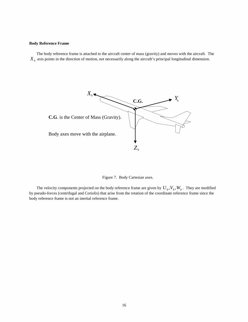
Body Reference Frame
The body reference frame is attached to the aircraft center of mass (gravity) and moves with the aircraft. The
bX axis points in the direction of motion, not necessarily along the aircraft’s principal longitudinal dimension.
Figure 7. Body Cartesian axes.
The velocity components projected on the body reference frame are given by bbb WVU ,, . They are modified by pseudo-forces (centrifugal and Coriolis) that arise from the rotation of the coordinate reference frame since the body reference frame is not an inertial reference frame.
X
Z
YC.G.b
b
b
C.G. is the Center of Mass (Gravity).
Body axes move with the airplane.
17
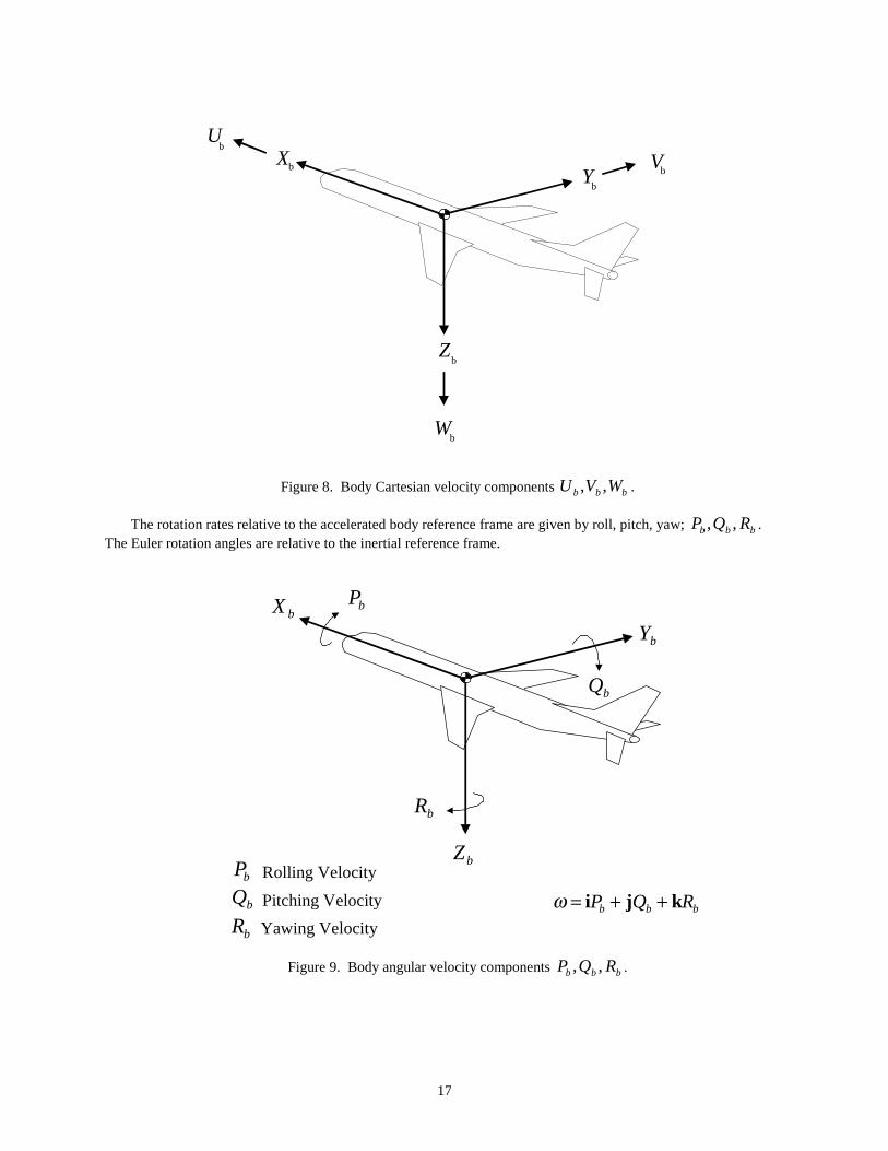
Figure 8. Body Cartesian velocity components bbb WVU ,, .
The rotation rates relative to the accelerated body reference frame are given by roll, pitch, yaw; bbb RQP ,, . The Euler rotation angles are relative to the inertial reference frame.
Figure 9. Body angular velocity components bbb RQP ,, .
X
Z
Y
W
VU
b
b
b
b
b
b
Rolling Velocity
Pitching Velocity
Yawing Velocitybbb R Q P kji ++ = ωbQ
bP
bR
bQ
bR
bPbX
bY
bZ
18
Inertial Reference Frame
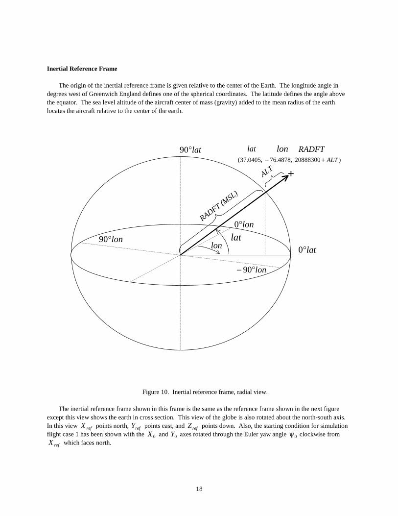
The origin of the inertial reference frame is given relative to the center of the Earth. The longitude angle in degrees west of Greenwich England defines one of the spherical coordinates. The latitude defines the angle above the equator. The sea level altitude of the aircraft center of mass (gravity) added to the mean radius of the earth locates the aircraft relative to the center of the earth.
Figure 10. Inertial reference frame, radial view.
The inertial reference frame shown in this frame is the same as the reference frame shown in the next figure except this view shows the earth in cross section. This view of the globe is also rotated about the north-south axis. In this view refX points north, refY points east, and refZ points down. Also, the starting condition for simulation flight case 1 has been shown with the 0X and 0Y axes rotated through the Euler yaw angle 0ψ clockwise from
refX which faces north.
lon°0
lat°0lon°90
) 20888300 76.4878, 37.0405,( ALT+−
+
lat lon RADFT
latlon
lon°− 90
lat°90
ALT
RADFT (MSL)
19
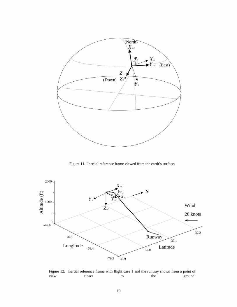
Figure 11. Inertial reference frame viewed from the earth’s surface.
Figure 12. Inertial reference frame with flight case 1 and the runway shown from a point of view closer to the ground.
X ref
Z ref
Y ref
0Ψ X 0
Y 0
Z 0
(North)
(East)
(Down)
0
2000
1000
-76.5
-76.4
36.9
37.1
37.0
37.2
-76.6
-76.3
N
Alti
tude
(ft)
LatitudeLongitude
Wind
20 knots
Runway
X ref
Y ref
Z ref
X 0
Y 0
0Ψ

20
The time histories of φθψ ,,,,, AltLonLat relative to the simulation origin reference axes refrefref ZYX ,,
defines the inertial position and orientation in figures 11 and 12. Figure 12 is a three dimensional Cartesian plot of the path of flight case 1 in latitude, longitude and altitude. Notice the orientation of north relative to figure 11.
Orientation Using Euler Angles
Figure 13. Airplane orientation using Euler angles.
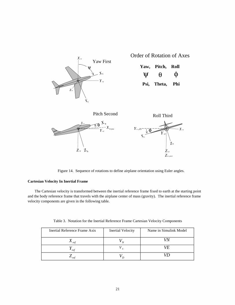
Figure 13 depicts the orientation of the vehicle. Start with the reference axes pointing north and east. The reference axes are fixed relative to the earth and form an inertial reference frame. The rotation of the earth is neglected in the B-737 Linear Autoland simulation. All the orientation Euler angle time histories refer to the inertial frame defined at the beginning of the simulation. The aircraft orientation is specified by three successive rotations relative to the reference axes. First, yaw the aircraft according to the Euler angle ψ . Second, pitch the aircraft using Euler angle θ . Third, roll the aircraft using Euler angle φ . The order of the rotations follows this convention and is important. Another order of successive rotations will give an incorrect orientation. The aircraft illustration is from [Ref. 12].
X ref
Z ref
Y ref
(North)
(East)
(Down)
Flight path
Earth-Fixed Axes
Order of Rotation of Axes
Yaw, Pitch, Roll
Psi, Theta, Phiψ θ φ
Y b
Zb
X b
Airplane Body Axes
21
Figure 14. Sequence of rotations to define airplane orientation using Euler angles.
Cartesian Velocity In Inertial Frame
The Cartesian velocity is transformed between the inertial reference frame fixed to earth at the starting point and the body reference frame that travels with the airplane center of mass (gravity). The inertial reference frame velocity components are given in the following table.
Table 3. Notation for the Inertial Reference Frame Cartesian Velocity Components
Inertial Reference Frame Axis
Inertial Velocity Name in Simulink Model
refX NV VN
refY EV VE
refZ DV VD
X ref
Z ref
Y ref
X b
Yb
ψ
Z ref
X ref θ X b
Z b Z ref
Y ref
Y ref
X b-yaw
Yb
φ
Z
X ref
b
Yaw First
Pitch Second Roll Third
Order of Rotation of Axes
Yaw, Pitch, Roll
Psi, Theta, Phi
ψ θ φ
Z pitchb−
Y pitchb−
22
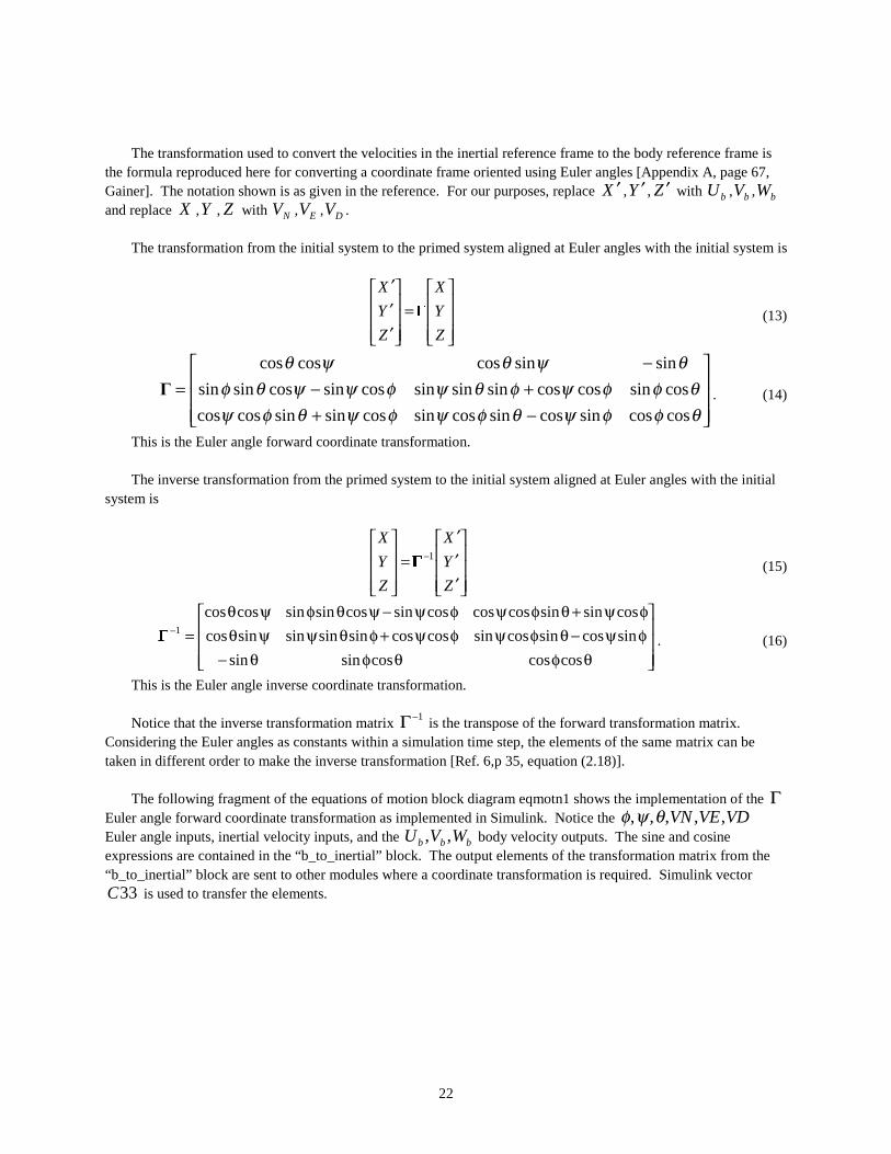
The transformation used to convert the velocities in the inertial reference frame to the body reference frame is the formula reproduced here for converting a coordinate frame oriented using Euler angles [Appendix A, page 67, Gainer]. The notation shown is as given in the reference. For our purposes, replace X ′ ,Y ′ , Z ′ with bU , bV , bW and replace X ,Y , Z with NV , EV , DV .
The transformation from the initial system to the primed system aligned at Euler angles with the initial system is
=
′′′
Z
Y
X
Z
Y
X
(13)
−++−
−=
θφφψθφψφψθφψθφφψφθψφψψθφ
θψθψθ
coscossincossincossincossinsincoscos
cossincoscossinsinsincossincossinsin
sinsincoscoscos
. (14)
This is the Euler angle forward coordinate transformation.
The inverse transformation from the primed system to the initial system aligned at Euler angles with the initial system is
′′′
=
−
Z
Y
X
Z
Y
X1
(15)
θφθφθ−φψ−θφψφψ+φθψψθφψ+θφψφψ−ψθφψθ
=−
coscoscossinsin
sincossincossincoscossinsinsinsincos
cossinsincoscoscossincossinsincoscos1
. (16)
This is the Euler angle inverse coordinate transformation.
Notice that the inverse transformation matrix 1−Γ is the transpose of the forward transformation matrix. Considering the Euler angles as constants within a simulation time step, the elements of the same matrix can be taken in different order to make the inverse transformation [Ref. 6,p 35, equation (2.18)].
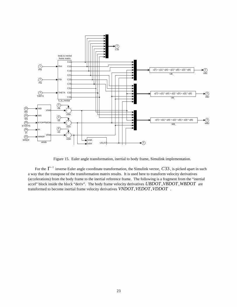
The following fragment of the equations of motion block diagram eqmotn1 shows the implementation of the Γ Euler angle forward coordinate transformation as implemented in Simulink. Notice the VDVEVN ,,,,, θψφ Euler angle inputs, inertial velocity inputs, and the bbb WVU ,, body velocity outputs. The sine and cosine expressions are contained in the “b_to_inertial” block. The output elements of the transformation matrix from the “b_to_inertial” block are sent to other modules where a coordinate transformation is required. Simulink vector
33C is used to transfer the elements.
23
Figure 15. Euler angle transformation, inertial to body frame, Simulink implementation.
For the 1−Γ inverse Euler angle coordinate transformation, the Simulink vector, 33C , is picked apart in such a way that the transpose of the transformation matrix results. It is used here to transform velocity derivatives (accelerations) from the body frame to the inertial reference frame. The following is a fragment from the “inertial accel” block inside the block “deriv”. The body frame velocity derivatives WBDOTVBDOTUBDOT ,, are transformed to become inertial frame velocity derivatives VDDOTVEDOTVNDOT ,, .
body to inertialframe matrix
5
4
C33
3
WB2
2
VB2
1
UB2
WD
WS
KTOFPS
PI
WINDF
VNW
VEW
VDW
windsVNR
VER UGUST
PHI
PSI
THETA
C11
C12
C13
C21
C22
C23
C31
C32
C33
b_to_inertial
u[7] + u[1] * u[4] + u[2] * u[5] + u[3] * u[6]
WB_
VNR
VER
VDR
u[7] + u[1] * u[4] + u[2] * u[5] + u[3] * u[6]
VB_
u[7] + u[1] * u[4] + u[2] * u[5] + u[3] * u[6]
UB_
24
PI
23
KTOFPS
12
WINDF
11
WS
10
WD
6
VD
5
VE
4
VN
3
THETA
2
PSI
1
PHI

24
Figure 16. Euler angle inverse transformation, body to inertial frame, Simulink implementation.
Angular Velocity In Inertial Frame
Figure 17. Angular velocity components.
body to inertialframe matrix 3
VDDOT
2
VEDOT
1
VNDOT
WBDOTP
u[1]*u[2] + u[3]*u[4] + u[5]*u[6]
u[1]*u[2] + u[3]*u[4] + u[5]*u[6]
u[1]*u[2] + u[3]*u[4] + u[5]*u[6]
VBDOTP
UBDOTP
u[1]*u[2] - u[3]*u[4]
u[1]*u[2] - u[3]*u[4]
u[1]*u[2] - u[3]*u[4]
5
C33
3
WBDOT
2
VBDOT
1
UBDOT
Rolling Velocity
Pitching Velocity
Yawing Velocity
bbb R Q P kji ++ = ω)(,, psidotRb ψ
)( , ,Qb thedotθ
)(,, phidotPb φ
ψθφ ,, Inertial frame
Body framebbb RQP ,,
bRbQbP
bXbY
bZ
25
Angular velocity in the inertial frame of reference is related to the angular velocity in the body frame according to the following transformation equations from [Ref. 6, p 102, equation (4.5,3)].
θψ−φ= sinbP
φθψ+φθ= sincoscos bQ (17)
φθ−φθψ= sincoscos bR For the special case where the Euler axes are lined up with the body axes, the rotational velocities agree across
the frames. The figure shows this special case. It is not that way in the model generally. The above equations are not seen in the model because the transformation of the Cartesian velocities takes care of this.
Autopilot Runway Frame
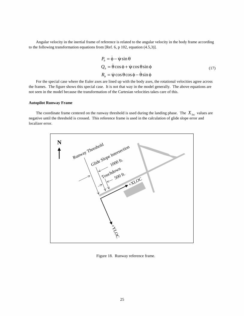
The coordinate frame centered on the runway threshold is used during the landing phase. The locX values are negative until the threshold is crossed. This reference frame is used in the calculation of glide slope error and localizer error.
Figure 18. Runway reference frame.
+XLOC
+YLO
C
Glide Slope Intersection
Runway Threshold
1000 ft.
500 ft.Touchdown
N
26
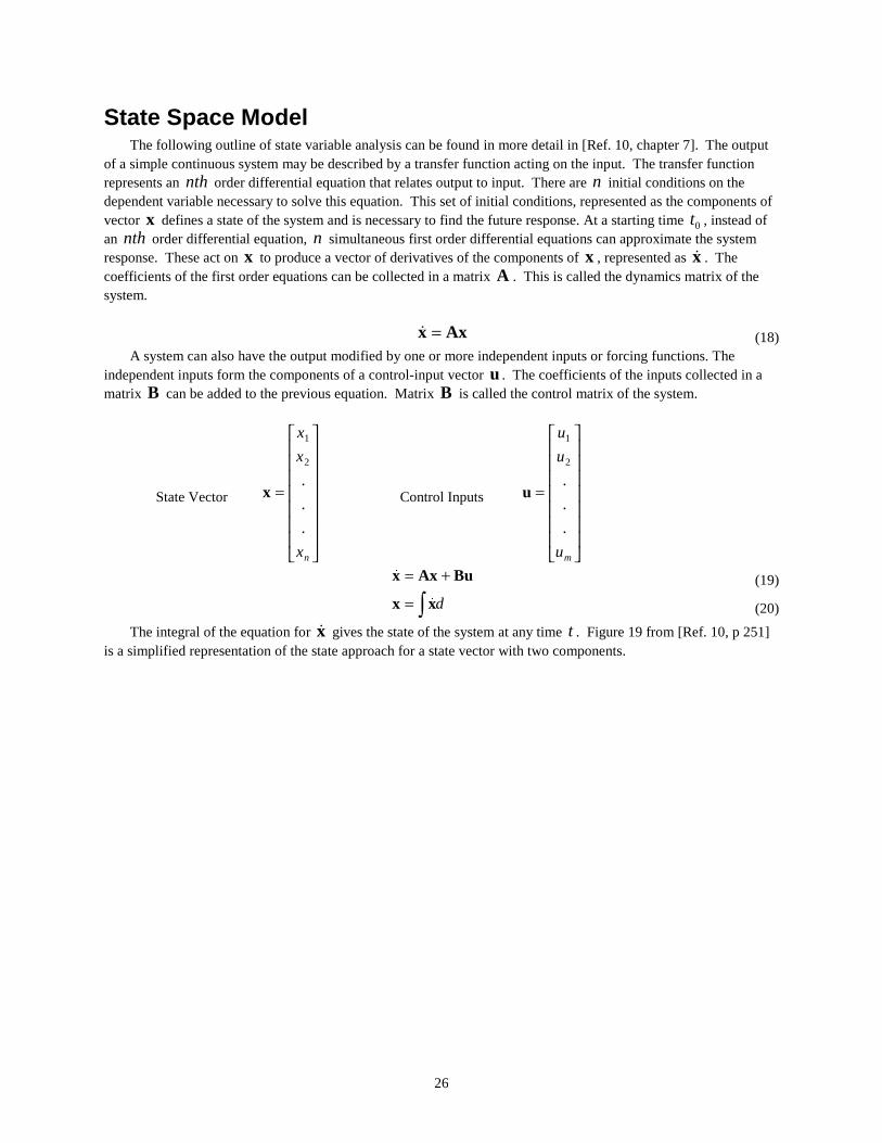
State Space Model The following outline of state variable analysis can be found in more detail in [Ref. 10, chapter 7]. The output
of a simple continuous system may be described by a transfer function acting on the input. The transfer function represents an nth order differential equation that relates output to input. There are n initial conditions on the dependent variable necessary to solve this equation. This set of initial conditions, represented as the components of vector x defines a state of the system and is necessary to find the future response. At a starting time 0t , instead of an nth order differential equation, n simultaneous first order differential equations can approximate the system response. These act on x to produce a vector of derivatives of the components of x , represented as x . The coefficients of the first order equations can be collected in a matrix A . This is called the dynamics matrix of the system.
Axx = (18) A system can also have the output modified by one or more independent inputs or forcing functions. The
independent inputs form the components of a control-input vector u . The coefficients of the inputs collected in a matrix B can be added to the previous equation. Matrix B is called the control matrix of the system.
State Vector
=
nx
x
x
.
.
.2
1
x Control Inputs
=
mu
u
u
.
.
.2
1
u
BuAxx += (19)
d∫= xx (20)
The integral of the equation for x gives the state of the system at any time t . Figure 19 from [Ref. 10, p 251] is a simplified representation of the state approach for a state vector with two components.

27
Figure 19. A state space trajectory with two independent variables.
Figure 20 shows the relationship in sequence between the A and B coefficient matrices from [Ref. 10, p 252]. The vector of control inputs, u , the vector of state derivatives, x , and the n simultaneous equations represented by the n parallel integrators produce a state vector x .
Figure 20. Data flow for a state space model.
1x
2x
)( 0tx
)(tx
)( ftxAx Bu
tx
ft
0t
0
State space
System trajectory
mu
u
u
.
.
.2
1
Controlinputs
nx
x
x
.
.
.2
1
Statevariables
n parallelintegrators
∫
A
Bu x x

28
State Vector Description
Figure 21 defines the components of the body state vector. The roll, pitch, and yaw Euler angles are considered body state parameters even though they are measured relative to the inertial reference frame fixed at the model starting point.
Figure 21. Body state vector components.
FORTRAN Common for State Vector
In the original Linear B-737 Autoland Simulation for Airlabs FORTRAN code, a key data structure is the global shared memory. The shaded portions show the body state vector and the derivative of the body state vector. Notice the “equivalence” statement that gives two names to the state vector variables. This is the heart of the original FORTRAN model. The differentiation and integration modules “deriv” and “ab2” use the “RSTATE” representation to iterate across all components of the body state vector in order to differentiate and integrate the simulation to get the next state value for the next time step.
ALT
P
R
V
Q
W
U
b
b
b
b
b
b
ψφ
θBodystatevector
x
Forward Velocity, Body Frame, (ft/sec)
Pitch Angular Velocity, Body Frame, (radians/sec)
Pitch Angle Relative to the Inertial Frame, (radians)
Side Velocity, Body Frame, (ft/sec)
Yaw Angular Velocity, Body Frame, (radians/sec)
Roll Angular Velocity, Body Frame, (radians/sec)
Altitude Above Mean Sea Level, (ft)
Down Velocity, Body Frame, (ft/sec)
Roll Angle Relative to the Inertial Frame, (radians)
Yaw Angle Relative to the Inertial Frame, (radians)

29
Figure 22. FORTRAN common block for state vector x and its derivative x .
Control Input Vector Description
This gives the definition of the components of the control input vector to the state space model. The aileron deflection and spoiler deflections come from the roll control system. The elevator deflection comes from the pitch control system. Both are actuator models. The rudder deflection comes from the yaw damper system. The stabilator position comes from the automatic stabilator trim system. The thrust comes from the engine model. The actuator models will be addressed in a subsequent section.
Figure 23. Control input vector components.
COMMON / CAB2 / * T , H , UB , WB , * QB , THETA , VB , RB , * PB , PHI , PSI , ALT , * LAT , LON , VN , VE , * VD , UBDOT , WBDOT , QBDOT , * THEDOT , VBDOT , RBDOT , PBDOT , * PHIDOT , PSIDOT , HDOT , DLAT , * DLON , VNDOT , VEDOT , VDDOTC DIMENSION RSTATE(10), RSTATED(10)C REAL * 8 LAT, LON, VN, VE, VD, DLAT, DLON, VNDOT, VEDOT, VDDOTC EQUIVALENCE (RSTATE (1), UB) EQUIVALENCE (RSTATED(1), UBDOT)
spl
spr
sp
thrust
r
a
e
δδ
δControl
input
vector
u
)(uvec
)(
)(
)(
delr
dela
dele
Engine Thrust, (lbs)
Stabilator Position, (pilot units)
Elevator Deflection, (deg)
Aileron Deflection, (deg)
Rudder Deflection, (deg)
Right Spoiler Deflection, (deg)
Left Spoiler Deflection, (deg)

30
FORTRAN Common for Control Input Vector
Like the state vector, the shaded portions show the control input vector in the Airlab FORTRAN model. Notice the “equivalence” statement that gives two names to the control vector variables. The differentiation module “deriv” uses the “UVEC” representation to iterate across all components of the control input vector in order to differentiate the state vector to get the next state derivative value for the next time step. The primary control inputs to the state space model listed here are not those that come out of the autopilot modules. Commanded throttle THROTLC, commanded elevator DELEC, commanded aileron DELAC, and commanded rudder DELRC come from the autopilot modules and are modified by the actuator models or other trim control systems like the stabilator trim or the yaw damper systems. There is a hierarchy of subsystems that surrounds the state space model.
Figure 24. FORTRAN common block for control vector u .
Inertial State Vector
Figure 25. Inertial state vector components.
COMMON / CDEFLEC / THRUST , SP , DELE , SPR ,
* DELA , DELR , SPL , UVEXTRA(3), * GEAR , FLAPS , E63 , E36 , * SBHP , EPR , THROTLCC DIMENSION UVEC(10)C EQUIVALENCE (UVEC(1), THRUST)
D
E
N
D
E
N
v
v
v
v
v
v
lon
lat
Inertial
state
vector
Latitude (deg)
Longitude (deg)
Velocity to the North, (ft/sec)
Velocity to the East, (ft/sec)
Velocity Downward, (ft/sec)
Acceleration to the North,
Acceleration to the East,
Acceleration Downward,
)(ft/sec2
)(ft/sec2
)(ft/sec2
31
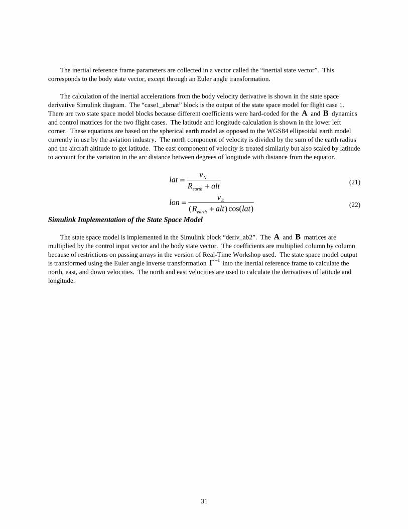
The inertial reference frame parameters are collected in a vector called the “inertial state vector”. This corresponds to the body state vector, except through an Euler angle transformation.
The calculation of the inertial accelerations from the body velocity derivative is shown in the state space derivative Simulink diagram. The “case1_abmat” block is the output of the state space model for flight case 1. There are two state space model blocks because different coefficients were hard-coded for the A and B dynamics and control matrices for the two flight cases. The latitude and longitude calculation is shown in the lower left corner. These equations are based on the spherical earth model as opposed to the WGS84 ellipsoidal earth model currently in use by the aviation industry. The north component of velocity is divided by the sum of the earth radius and the aircraft altitude to get latitude. The east component of velocity is treated similarly but also scaled by latitude to account for the variation in the arc distance between degrees of longitude with distance from the equator.
altR
vlat
earth
N
+= (21)
)cos()( lataltR
vlon
earth
E
+= (22)
Simulink Implementation of the State Space Model
The state space model is implemented in the Simulink block “deriv_ab2”. The A and B matrices are multiplied by the control input vector and the body state vector. The coefficients are multiplied column by column because of restrictions on passing arrays in the version of Real-Time Workshop used. The state space model output is transformed using the Euler angle inverse transformation 1−Γ into the inertial reference frame to calculate the north, east, and down velocities. The north and east velocities are used to calculate the derivatives of latitude and longitude.
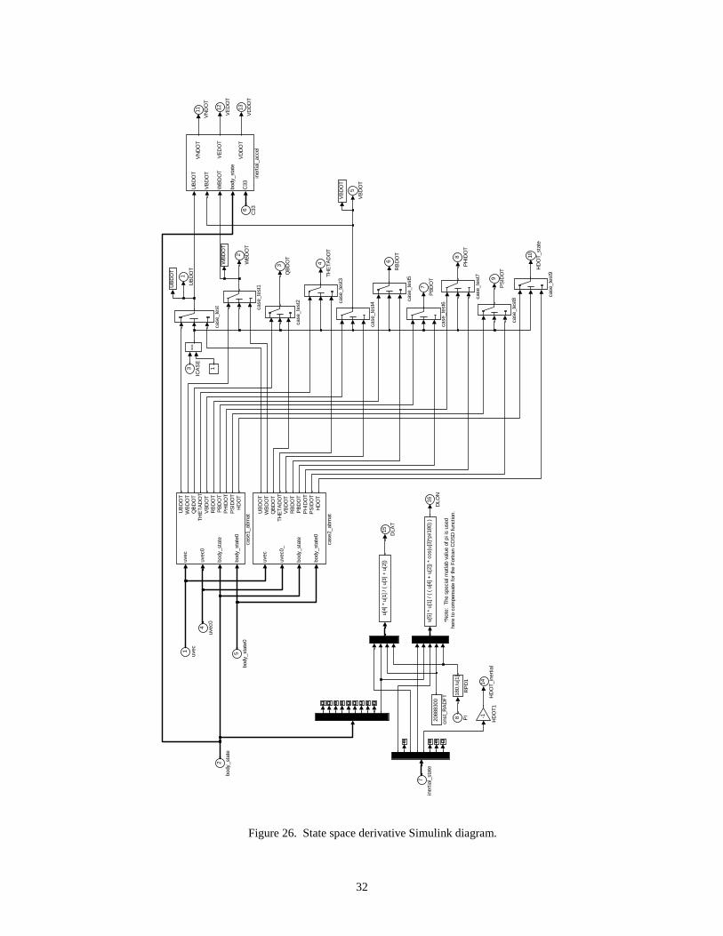
32
Figure 26. State space derivative Simulink diagram.
*Not
e: T
he s
peci
al m
atla
b va
lue
of p
i is
used
here
to c
ompe
nsat
e fo
r th
e F
ortr
an C
OS
D fu
nctio
n.
16
DLO
N
15
DLA
T
14
HD
OT
_ine
rtia
l
13
VD
DO
T
12
VE
DO
T
11
VN
DO
T
10
HD
OT
_sta
te
9
PS
IDO
T
8
PH
IDO
T
7
PB
DO
T
6
RB
DO
T
5
VB
DO
T
4
TH
ET
AD
OT
3
QB
DO
T
2
WB
DO
T
1
UB
DO
T==
UB
DO
T
VB
DO
T
WB
DO
T
body
_sta
te
C33
VN
DO
T
VE
DO
T
VD
DO
T
iner
tial_
acce
l
WB
DO
T
VB
DO
T
UB
DO
T
2088
8300
cnst
_RA
DF
T
case
_tes
t9
case
_tes
t8case
_tes
t7
case
_tes
t6
case
_tes
t5
case
_tes
t4case
_tes
t3
case
_tes
t2
case
_tes
t1
case
_tes
t
uvec
uvec
0_
body
_sta
te
body
_sta
te0
UB
DO
TW
BD
OT
QB
DO
TT
HE
TA
DO
TV
BD
OT
RB
DO
TP
BD
OT
PH
IDO
TP
SID
OT
HD
OT
case
2_ab
mat
uvec
uvec
0
body
_sta
te
body
_sta
te0
UB
DO
TW
BD
OT
QB
DO
TT
HE
TA
DO
TV
BD
OT
RB
DO
TP
BD
OT
PH
IDO
TP
SID
OT
HD
OT
case
1_ab
mat
180.
/u[1
]
RP
D1
-1
HD
OT
1
u[5]
* u
[1] /
( (
u[4
] +
u[2]
) *
cos(
u[3]
*pi/1
80)
)
u[4]
* u
[1] /
( u
[3] +
u[2
])
1
8 PI
7
iner
tial_
stat
e
6
C33
5
body
_sta
te0
4
uvec
0
3
ICA
SE
2
body
_sta
te
1
uvec
33
The latitude, longitude, north, east, and down velocities are part of the inertial reference frame description of the airplane state. The inertial velocities are not part of the state matrix simultaneous first order differential equations as defined in the B-737 Autoland model. The Newtonian laws of motion that relate change in momentum to force on a body assume an inertial reference frame (one that is not accelerated or rotating). Calculations are made with respect to an inertial reference frame and the non-inertial body reference frame. It is more convenient to calculate moments of inertia from non-inertial body reference frame as shown in the section on simplified torque calculation.
The body reference frame is not an inertial reference frame and exhibits fictitious forces due to its acceleration. The fictitious forces that are an artifact of rotation are the centrifugal and Coriolis forces. The laws of motion need to be modified to account for these. A side calculation uses the output of the body state vector to calculate the body acceleration components from the body velocity derivative. These are converted to acceleration components in the inertial reference frame. These inertial acceleration components are integrated to get inertial velocities for the next time step. The velocities are integrated to get inertial position coordinates, latitude and longitude, for the next time step. Finally, the inertial velocities are transformed into body velocities using the Euler angle coordinate transformation Γ . In this way, the centrifugal and Coriolis forces are accounted for. This is what makes the order of calculation important.
Equations of Motion The equations of motion module contains four component modules. Module “eqmotn1” contains the
transformation of velocity from the inertial reference frame to the body reference frame using the Euler angle transformation matrix. The effect of winds and gusts is applied in this block as well. The Dryden gust model contained here will be discussed in a subsequent section.
The module “eqmotn2” calculates the angle of attack α , sideslip angle β , various airspeeds, atmosphere state parameters, and Mach number. The angle of attack and sideslip angle are a simple trigonometric calculation based on body velocity components. The atmosphere state parameters come from a polynomial function of altitude [Ref. 21]. Density, temperature, pressure and speed of sound are obtained in this way. Total body velocity, true air speed, and calibrated airspeed are calculated from the body velocity components and Mach number corrections. The following contains definitions of the different air speeds as shown in [Ref. 2, p 4-6].

34
Table 4. Air Speed Definitions
Airspeed Meaning of Name Definition
IAS Indicated Airspeed Measured using a pitot tube and static port to get the difference between total pressure and static pressure. The pilot’s instrument is calibrated to read this.
CAS Calibrated Airspeed The measured pitot and static port readings are corrected to account for the pitot tube being not aligned with the airstream at a non-zero angle of attack. Other instrumentation and installation errors are accounted for.
TAS True Airspeed Actual speed at which the aircraft moves through the air. CAS is corrected for non standard temperature and pressure.
MACH Mach Number Ratio of true airspeed to the speed of sound.
Localizer and Glide Slope Error
The module “eqmotn3’ calculates the position of the aircraft relative to the runway reference frame to support the instrument landing system (ILS) for the Autoland. The latitude, longitude, altitude, earth radius, and runway position coordinates are used to calculate the position of the aircraft in the runway reference frame. The aircraft center of mass (gravity) position components in the runway frame are ),,( cgcgcg HYX . Simple trigonometry is used to calculate the glide slope error GSE and the track error ETA for the ILS.
35
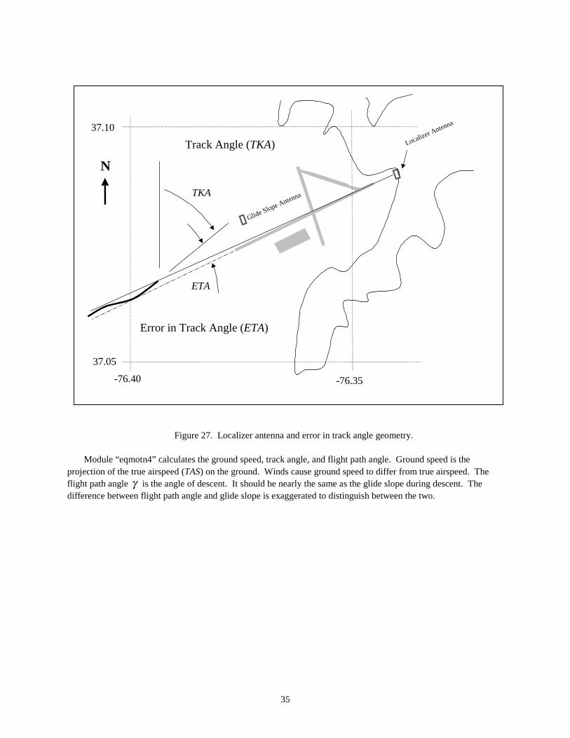
Figure 27. Localizer antenna and error in track angle geometry.
Module “eqmotn4” calculates the ground speed, track angle, and flight path angle. Ground speed is the projection of the true airspeed (TAS) on the ground. Winds cause ground speed to differ from true airspeed. The flight path angle γ is the angle of descent. It should be nearly the same as the glide slope during descent. The difference between flight path angle and glide slope is exaggerated to distinguish between the two.
-76.40 -76.35
37.05
37.10
Localizer Antenna
Glide Slope Antenna
N
Error in Track Angle (ETA)
ETA
Track Angle (TKA)
TKA

36
Figure 28. Glide slope error (GSE) and flight path angle .
0
Alti
tude
(ft
)
1000
-76.5
-76.4
36.9
37.1
Latitude
Longitude37.0
37.2
-76.6
-76.3
N
Glide Slope
GSE
γ
(parallel to runway)
Runway
37
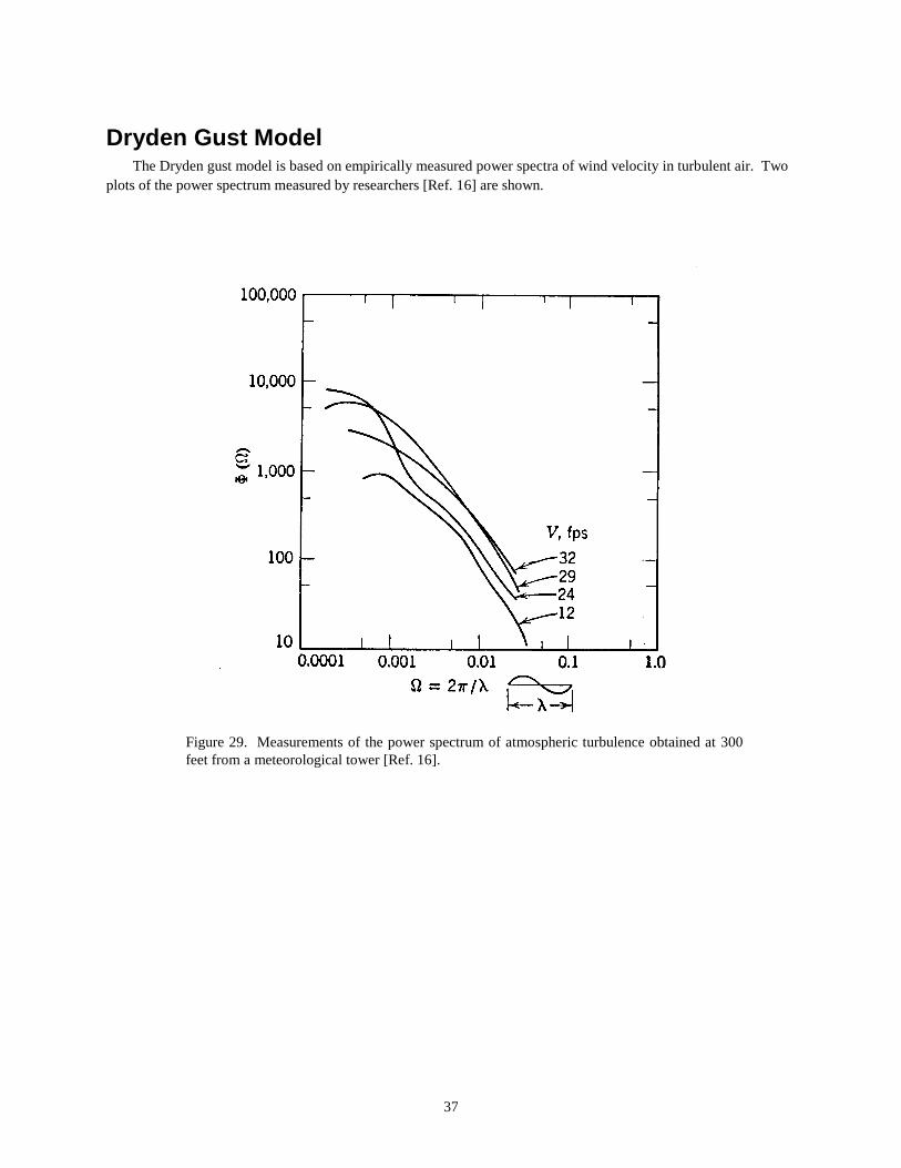
Dryden Gust Model The Dryden gust model is based on empirically measured power spectra of wind velocity in turbulent air. Two
plots of the power spectrum measured by researchers [Ref. 16] are shown.
Figure 29. Measurements of the power spectrum of atmospheric turbulence obtained at 300 feet from a meteorological tower [Ref. 16].
38
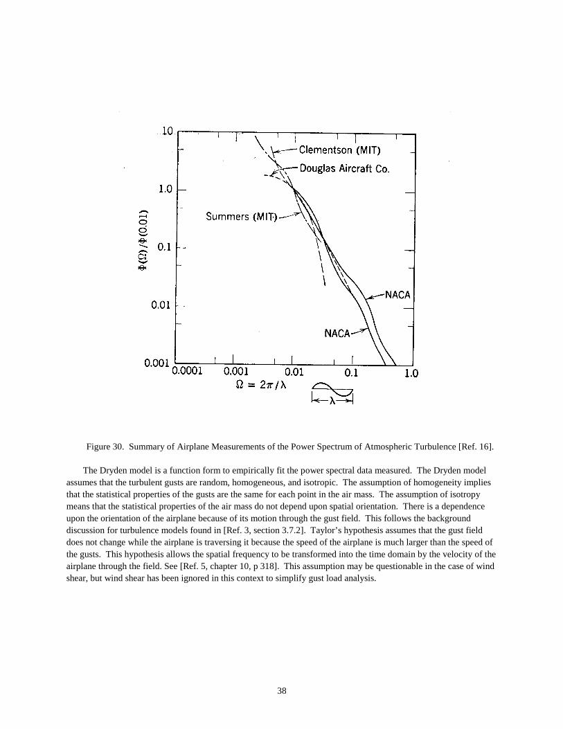
Figure 30. Summary of Airplane Measurements of the Power Spectrum of Atmospheric Turbulence [Ref. 16].
The Dryden model is a function form to empirically fit the power spectral data measured. The Dryden model assumes that the turbulent gusts are random, homogeneous, and isotropic. The assumption of homogeneity implies that the statistical properties of the gusts are the same for each point in the air mass. The assumption of isotropy means that the statistical properties of the air mass do not depend upon spatial orientation. There is a dependence upon the orientation of the airplane because of its motion through the gust field. This follows the background discussion for turbulence models found in [Ref. 3, section 3.7.2]. Taylor’s hypothesis assumes that the gust field does not change while the airplane is traversing it because the speed of the airplane is much larger than the speed of the gusts. This hypothesis allows the spatial frequency to be transformed into the time domain by the velocity of the airplane through the field. See [Ref. 5, chapter 10, p 318]. This assumption may be questionable in the case of wind shear, but wind shear has been ignored in this context to simplify gust load analysis.
39
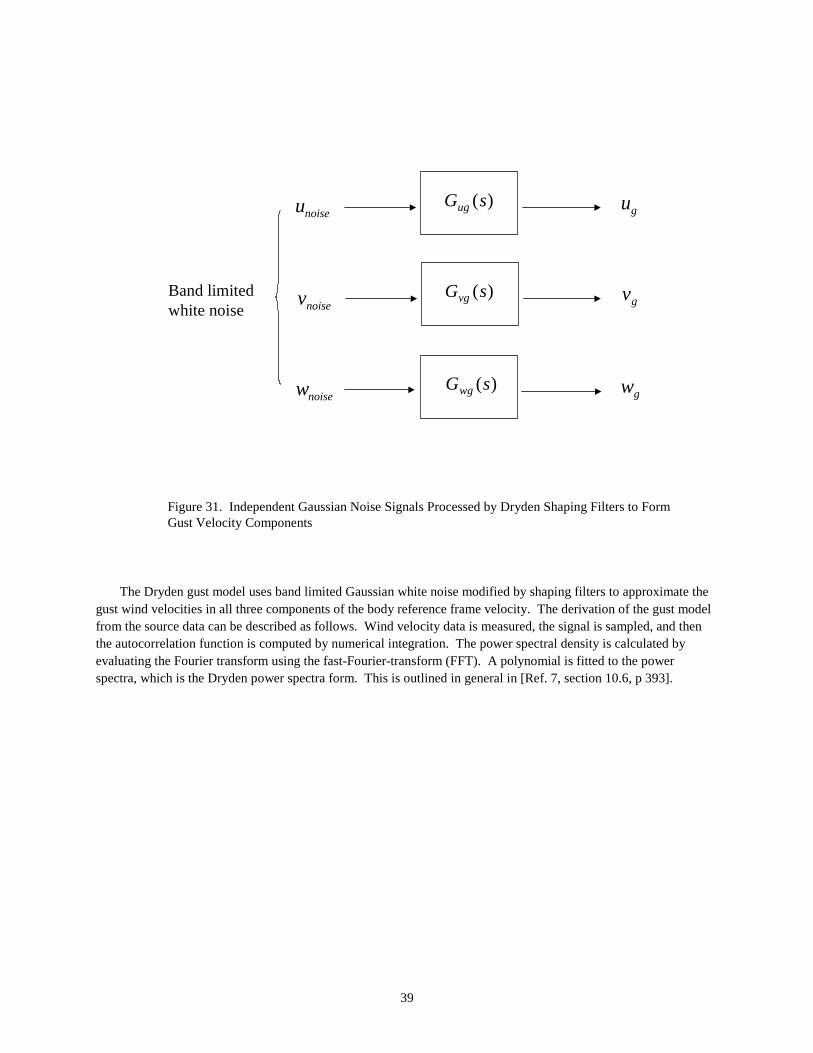
Figure 31. Independent Gaussian Noise Signals Processed by Dryden Shaping Filters to Form Gust Velocity Components
The Dryden gust model uses band limited Gaussian white noise modified by shaping filters to approximate the gust wind velocities in all three components of the body reference frame velocity. The derivation of the gust model from the source data can be described as follows. Wind velocity data is measured, the signal is sampled, and then the autocorrelation function is computed by numerical integration. The power spectral density is calculated by evaluating the Fourier transform using the fast-Fourier-transform (FFT). A polynomial is fitted to the power spectra, which is the Dryden power spectra form. This is outlined in general in [Ref. 7, section 10.6, p 393].
)(sGug gu
Band limitedwhite noise
)(sGvg gv
)(sGwg gw
noiseu
noisev
noisew

40
Dryden Gust Model Notation
Table 5. Dryden Gust Model Notation HCG Height of the aircraft center of mass (gravity) above ground level. (ft)
uS
vS
wS
Power spectral density
Ω Spatial frequency (cycles/ft)
uL
vL
wL
Length scale for gust velocity for all three components (ft) Length scaling for clear air < 1750 ft
3
1
145 )(HCGLu =
3
1
145 )(HCGLv =
HCGLw =
0V Magnitude of apparent wind velocity from the motion of the aircraft relative to the air mass (inertial velocity adjusted to account for steady wind velocity components)
windinertialV VV −=0
uσ
vσ
wσ
Root mean square gust magnitude. (ft/sec)
ΩΩ= ∫+∞
∞−
dS )(2σ
The U and V components are the same as the input gust magnitude. The W component is scaled by the cube root of the altitude measured from the aircraft center of gravity in feet. This accounts for the boundary condition of zero vertical motion of the gust in contact with the ground.
3
1
145)(HCGu
w
σ=σ
41
The autocorrelation functions of the Dryden gust model from [Ref. 1, p 42, fig.120] are:
u
g
Lu eR
τ
τ−
=)(
−=
−
v
Lv L
eR v
g 21)(
τττ
(23)
−=
−
w
Lw L
eR w
g 21)(
τττ
The power spectrum functions for the Dryden gust spectra are:
2
2
)(1
1)(
Ω+=Ω
u
uuu L
LS
g πσ
[ ]22
22
1
31
2 )(
)()(
Ω+
Ω+π
σ=Ωv
vvvv
L
LLS
g (24)
[ ]22
22
1
31
2 )(
)()(
Ω+
Ω+π
σ=Ωw
wwww
L
LLS
g
)(ΩgvS and )(Ω
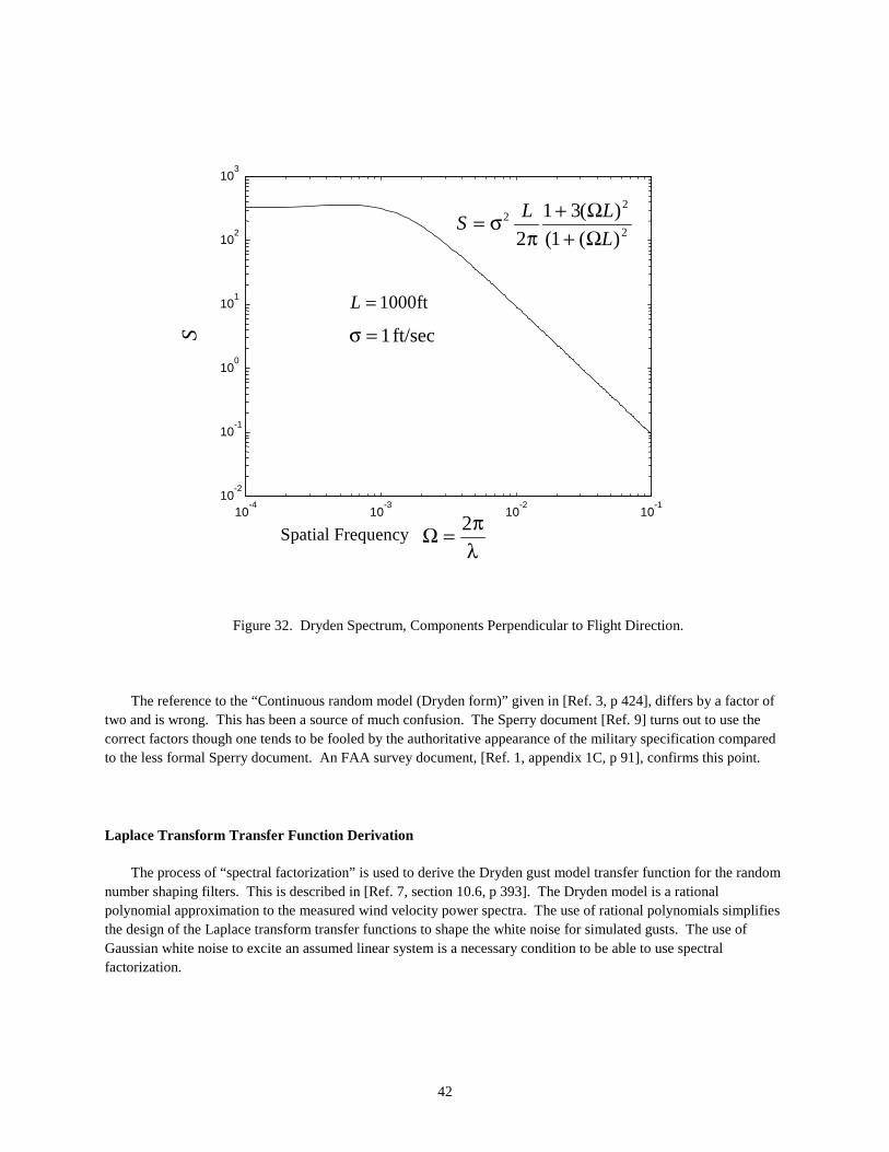
gwS are of the form of the equation for the lateral one-dimensional spectra given in [Ref. 6, p 318, equation (10.3,12)]. Here is a plot of the v and w component power spectra produced by the Dryden power spectrum functional form.
42
Figure 32. Dryden Spectrum, Components Perpendicular to Flight Direction.
The reference to the “Continuous random model (Dryden form)” given in [Ref. 3, p 424], differs by a factor of two and is wrong. This has been a source of much confusion. The Sperry document [Ref. 9] turns out to use the correct factors though one tends to be fooled by the authoritative appearance of the military specification compared to the less formal Sperry document. An FAA survey document, [Ref. 1, appendix 1C, p 91], confirms this point.
Laplace Transform Transfer Function Derivation
The process of “spectral factorization” is used to derive the Dryden gust model transfer function for the random number shaping filters. This is described in [Ref. 7, section 10.6, p 393]. The Dryden model is a rational polynomial approximation to the measured wind velocity power spectra. The use of rational polynomials simplifies the design of the Laplace transform transfer functions to shape the white noise for simulated gusts. The use of Gaussian white noise to excite an assumed linear system is a necessary condition to be able to use spectral factorization.
10-4
10-3
10-2
10-1
10-2
10-1
100
101
102
103
2
22
)(1(
)(31
2 L
LLS
Ω+Ω+
πσ=
λπ=Ω 2
S
ft1000=L
ft/sec 1=σ
Spatial Frequency

43
To perform spectral factorization, the power spectrum is first written as a function of 2ω .
2
0
0
2
1
1)(
+
=
ωπ
σω
V
LV
LS
u
uuug
22
0
2
0
0
2
1
31
2)(
+
+
=
ω
ω
πσω
V
L
V
L
V
LS
v
v
vvvg (25)
22
0
2
0
0
2
1
31
2)(
+
+
=
ω
ω
πσω
V
L
V
L
V
LS
w
w
wwwg
The notation to describe a linear system undergoing a single impulse input is given here to be consistent with
that in [Ref. 7] on spectral factorization. This will be an expanded derivation from that shown in [Ref. 7] applied to the special case of the Dryden gust model. The case of a single scalar input and output modified by a transfer function will be considered as the gust component shaping filter. The function )(tH is the response of the linear
system to an impulse as input. The Laplace transform of the impulse response is the system transfer function in the complex frequency plane s . The response of the system to random input is also considered. Gaussian white noise is a special form of random input used to simplify the spectral analysis of the system’s frequency response. Gaussian white noise has a mean of zero and a flat power spectrum. Use of the white noise abstraction permits simple expressions for the output of the system in the time and frequency domains. The following relations for a linear system come from [Ref. 7, p 390].

44
Figure 33. Linear system input-output relationship
Table 6. Laplace Transform Notation )(tH Impulse response in the time domain
)(s , )]([ tH Transfer function in the frequency domain
Table 7. Input-output Relation for Linear System with Deterministic Input and with White Noise Input
Domain
Deterministic inputs
White noise inputs
Time domain
τ−=λ
λλλ−= ∫t
dutHtyt
0
)()()(
∫∞
ξτ+ξ′ξ=τ0
dHQHRy )()()(
Frequency domain
))() u(ssy(s =
)()()( ωωω jQjS y ′−=
Input
uH
Output
y
Linear System

45
Spectral Factorization
A transfer function expressed in the Laplace transform complex frequency domain s is the transform of the output function divided by the transform of the input function.
)
))(
(s
(ss
= (26)
[Ref. 7, p 393, 394] shows the process of expressing )H(s as the ratio of polynomials in s , then as a ratio of polynomials in 2ω .
kkk
kkk
ss
ss
(s
(ss
ααβββ
++++++== −
−−
...
...
)
))H(
11
21
11
(27)
To perform spectral factorization, reverse the process. Begin with the spectrum expressed as a ratio of polynomials in 2ω . Factor the expressions in the numerator and denominator,
))...()((
))...()((
)
))(
21
121
k
k
pspsps
zszszsc
(s
(ss
−−−−−−== −
(28)
then solve for poles and zeros. Set each factor to zero to find a root of the equation. Roots in the denominator are poles of the transfer function, and roots in the numerator are zeros. Choose the square root for the zero and pole expressions to keep the transfer function in the stable part of the complex plane, the left half-plane. Choose the square root with the positive real part in the numerator and denominator in order to make )H(s have poles and zeros in the left half-plane. This is called the “minimum phase” factorization [Ref. 7, p 395].
Figure 34. Complex frequency plane
O
ωj
σ
ωσ js +=
Want Poles and Zeros to be Here
46
Step 1.
Write yS as a rational function of 2ω . To be specific, the transfer function for the gu component of the
Dryden gust velocity will be calculated. The power spectral density as a rational function of 2ω is:
2
2
0
0
2
1
1)(
ωπ
σω
+
=
V
LV
LS
u
uuug (29)
Define the numerator function,
1)( 2 =ωN (30) and define the denominator function.
2
2
0
2 1)( ωω
+=
V
LD u
(31)
Both are rational functions in 2ω .
Step 2.
Find the roots of )( 2ωN and )( 2ωD
Using the factor theorem from the algebra of nth degree equations from [page 224, Eshbach]:
0)( 110 =+++= −
nnn axaxaxf (32)
If, and only if, )( rx − is a factor of )(xf , then 0)( =rf .
First, solve for roots in the numerator.
Numerator: 1)( 2 =ωN (33)
Notice that the numerator is a constant for all ω . Next, solve for roots in the denominator.
Denominator: 2
2
0
2 1 ω
+=ω
V
LD u)( (34)
))...()(()( kD β−ωβ−ωβ−ω=ω 22
21
22
(35)
47
Taking the first one of the factors,
)( 12 β−ω
To cast the right hand side of equation (34) into this form,
2
2
0
10 ω
+=
V
Lu
2
2
0
0 ω+
=
−
V
Lu
2
0
20−
−−ω=
V
Lu)(
2
0
−
−=
V
Luβ (36)
Step 3. Find the poles and zeros of the transfer function.
Pole of the transfer function β=1p (37)
1
01
−
±=
V
Ljp u
(38)
Make necessary factorization to keep imaginary part on ω .
β−ω= 20
))(( β+ωβ−ω=0
+ω⋅
−ω=
−− 1
0
1
0
0V
Lj
V
Lj uu
+ω
⋅
−ω
= 110
00
jV
Lj
V
L uu
Substitute the result of the pole and zero calculation back into the power spectral density formula given white
noise input.
48
)()()( ωωω jQjSgu ′−= (39)
)()(
)()()(
2221
2
21
221
22
k
ku
pp
zzQcS
g −ω−ω−ω−ω
=ω −
)()(
)()(
)()(
)()()(
k
k
k
ku pjpj
zjzj
pjpj
zjzjQcS
g −ω−ω−ω−ω
⋅−ω−−ω−
−ω−−ω−=ω −−
1
11
1
112 (40)
Make the substitution using the factorized denominator.
−ω
⋅
+ω
=ω
1
1
1
1
00
2
jV
Lj
V
LQcS
uu
ug)( (41)
Place the factor in the position for the transfer function )(s . Use the factor that does not have poles in the
right half of the complex plane.
Step 4.
Choose the transfer function filter gain c . Let the spectral density of the white noise factor, Q , be unity for
now. It will be accounted for later. Choose Q to be 1 and 2c to be 0
2
V
Luu π
σ . The transfer function that results is
used to make the longitudinal gust velocity component shaping filter.
+
=
1
1)(
0
0s
V
LV
Ls
u
uuug π
σ (42)
The transfer function for the lateral and vertical gust velocity components can be derived in a similar manner.
2
0
0
01
31
2)(
+
+=
sV
L
sV
L
V
Ls
v
v
vvvg π
σ (43)
2
0
0
01
31
2)(
+
+=
sV
L
sV
L
V
Ls
w
w
wwwg π
σ (44)
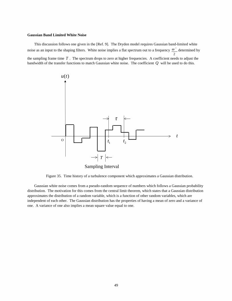
49
Gaussian Band Limited White Noise
This discussion follows one given in the [Ref. 9]. The Dryden model requires Gaussian band-limited white
noise as an input to the shaping filters. White noise implies a flat spectrum out to a frequency 2
∗ω determined by
the sampling frame time T . The spectrum drops to zero at higher frequencies. A coefficient needs to adjust the bandwidth of the transfer functions to match Gaussian white noise. The coefficient Q will be used to do this.
Figure 35. Time history of a turbulence component which approximates a Gaussian distribution.
Gaussian white noise comes from a pseudo-random sequence of numbers which follows a Gaussian probability distribution. The motivation for this comes from the central limit theorem, which states that a Gaussian distribution approximates the distribution of a random variable, which is a function of other random variables, which are independent of each other. The Gaussian distribution has the properties of having a mean of zero and a variance of one. A variance of one also implies a mean square value equal to one.
O
)(tu
t
T
Sampling Interval
1t 2t
τ
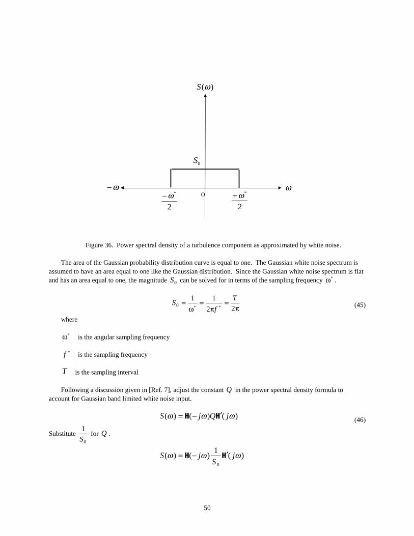
50
Figure 36. Power spectral density of a turbulence component as approximated by white noise.
The area of the Gaussian probability distribution curve is equal to one. The Gaussian white noise spectrum is assumed to have an area equal to one like the Gaussian distribution. Since the Gaussian white noise spectrum is flat and has an area equal to one, the magnitude 0S can be solved for in terms of the sampling frequency ∗ω .
π=
π=
ω=
∗∗ 22
110
T
fS (45)
where
∗ω is the angular sampling frequency
∗f is the sampling frequency
T is the sampling interval
Following a discussion given in [Ref. 7], adjust the constant Q in the power spectral density formula to account for Gaussian band limited white noise input.
)()()( ωωω jQjS ′−= (46)
Substitute 0
1
S for Q .
)(1
)()(0
ωωω jS
jS ′−=
O
)(ωS
ω
2
*ω+2
*ω−
0S
ω−

51
)(1
)(1
)(00
ωωω jS
jS
S ′−=
Substitute for the coefficient 0S from equation (45).
)(2
)(2
)( ωπωπω jT
jT
S ′−=
Define the coefficients to be part of the transfer function for the shaping filters.
)()()( ωωω jjS ′−= (47)
The shaping filter transfer functions with the new coefficients for each gust component are:
+
=
1
12)(
0
0s
V
LTV
Ls
u
uuu σ (48)
2
0
0
01
31
)(
+
+=
sV
L
sV
L
TV
Ls
v
v
vvv σ (49)
2
0
0
01
31
)(
+
+=
sV
L
sV
L
TV
Ls
w
w
www σ (50)

52
Figure 37. Independent Gaussian noise signals processed by Dryden shaping filters to form gust velocity components.
)(G su gu
Band limitedwhite noise
)(G sv gv
)(G sw gw
noiseu
noisev
noisew

53
Z-transform Transfer Function Derivation
This derivation is expanded from that given in [Ref. 9]. The discrete Z-transform function expression of the Dryden gust model starts off as a modified Laplace transform model. The gust model shaping filter is split into two cascaded filters evaluated in series for the v and the w gust components. The first is called the lag filter and the second the lag lead filter.
Figure 38. Lag and lag lead filters to replace each shaping filter.
Table 8. Constants for the Series Lag and the Series Lag Lead Filters. u v w
α uβ
3
1 vβ
3
1 wβ
3
1
β
uL
V0 vL
V0 wL
V0
gu
gv
gw
Lag filter
Lag filter
Lag filter
Lag leadfilter
Lag leadfilter
noiseu
noisev
noisew

54
Figure 39. Lag and lead lag filters replace each shaping filter.
The Laplace transform frequency domain expressions for the lag and lead lag filters are found in figure 39. The Z-transform implementation of the continuous lag and lag lead filters follows. First, modify the notation of input and output to a linear system to match that used in [Ref. 15].
Figure 40. Linear system with transfer function )(s .
To convert from the Gaussian white noise input to the gust component output, a transfer function represented by )(s is used. This was derived from the Dryden theory of wind gusts through the process of spectral factorization.
gu
gv
gw
noiseu
noisev
noisew
uu Tβσ 2
us β+1
vs β+1
ws β+1
v
v
s
s
βα
++
w
w
s
s
β+α+
coeffu
vv Tβσ 2
coeffv
ww Tβσ 2
coeffw
Lag
Lag Lead
)(tu
)U(s)G(s
)(ty
)Y(s

55
Figure 41. Sampled equivalent of a linear system with transfer function )(s .
Figure 41 shows the linear system with the triangular hold transfer function added in series. The linear system has a continuous function input )(tu that is represented by the graph in figure 42(a). The
asterisk notation means “a sample of”. The switch represents a digital sampler. An equivalent ideal sampler can be imagined to exist and is represented mathematically by a train of delta functions of unit amplitude occurring at T instants in time. See figure 42(b). The same thing shown symbolically is:
)(...)()()()()( kTtTtTtTtttT −δ++−δ+−δ+−δ+−δ=δ 320
∑∞
=
−δ=δ0k
T kTtt )()( (51)
The function )(tu when sampled at the T instants in time can be thought of as being the product of
the value of the continuous function and the delta function. This new function is given the name )(tu∗
using the asterisk notation. This train of scaled impulses is shown in figure 42(c). )(tu∗ shown
symbolically is:
)()(...)()()()()()()( kTtkTuTtTuTtTututu −δ++−δ+−δ+−δ=∗ 2200
Which is an infinite series expressed as:
∑∞
=
∗ −δ=0k
kTtkTutu )()()( (52)
To solve the differential control equations algebraically, the Laplace transform representation is useful. It transforms the equations in time to be equations in the complex frequency plane s. The definition of the Laplace transform is:
[ ] ∫ −== dttuestu ts )()()( (53)
)(tu
)U(s)(H s∆
)(ty
)Y(s)G(s
)(ty∗
)(Y s∗
)(tu∗
)(U s∗
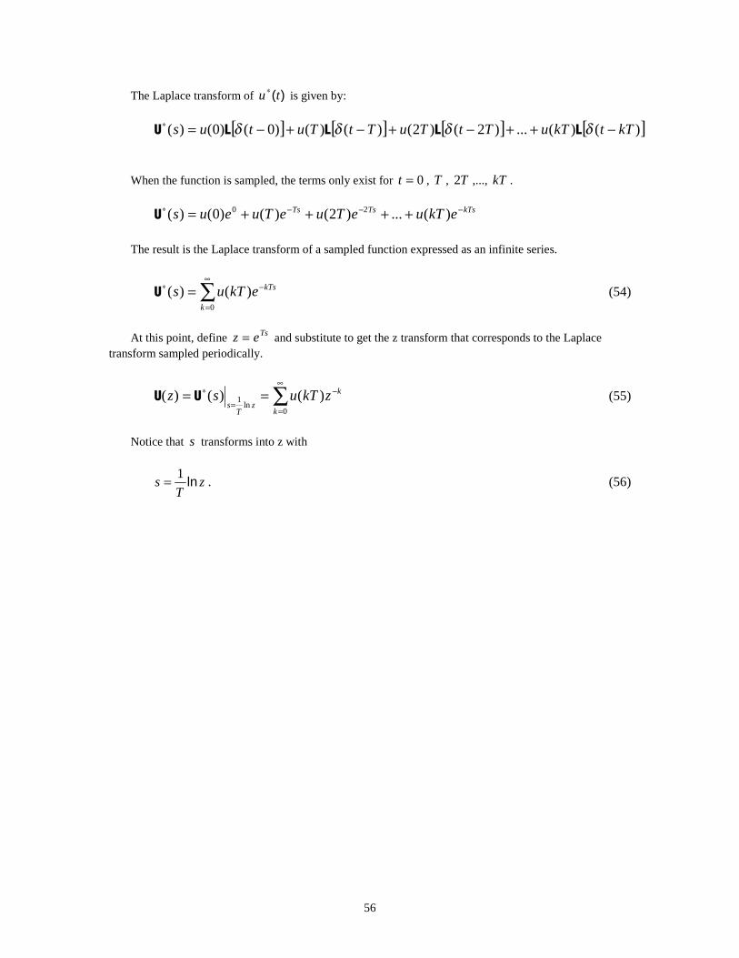
56
The Laplace transform of )(tu∗ is given by:
[ ] [ ] [ ] [ ])()(...)2()2()()()0()0()( kTtkTuTtTuTtTutus −++−+−+−=∗ δδδδ
When the function is sampled, the terms only exist for 0=t , T , T2 ,..., kT .
kTsTsTs ekTueTueTueus −−−∗ ++++= )(...)2()()0()( 20
The result is the Laplace transform of a sampled function expressed as an infinite series.
∑∞
=
−∗ =0
)()(k
kTsekTus (54)
At this point, define Tsez = and substitute to get the z transform that corresponds to the Laplace transform sampled periodically.
∑∞
=
−
=
∗ ==0
ln1 )()()(
k
k
zT
szkTusz (55)
Notice that s transforms into z with
zT
s ln1= . (56)
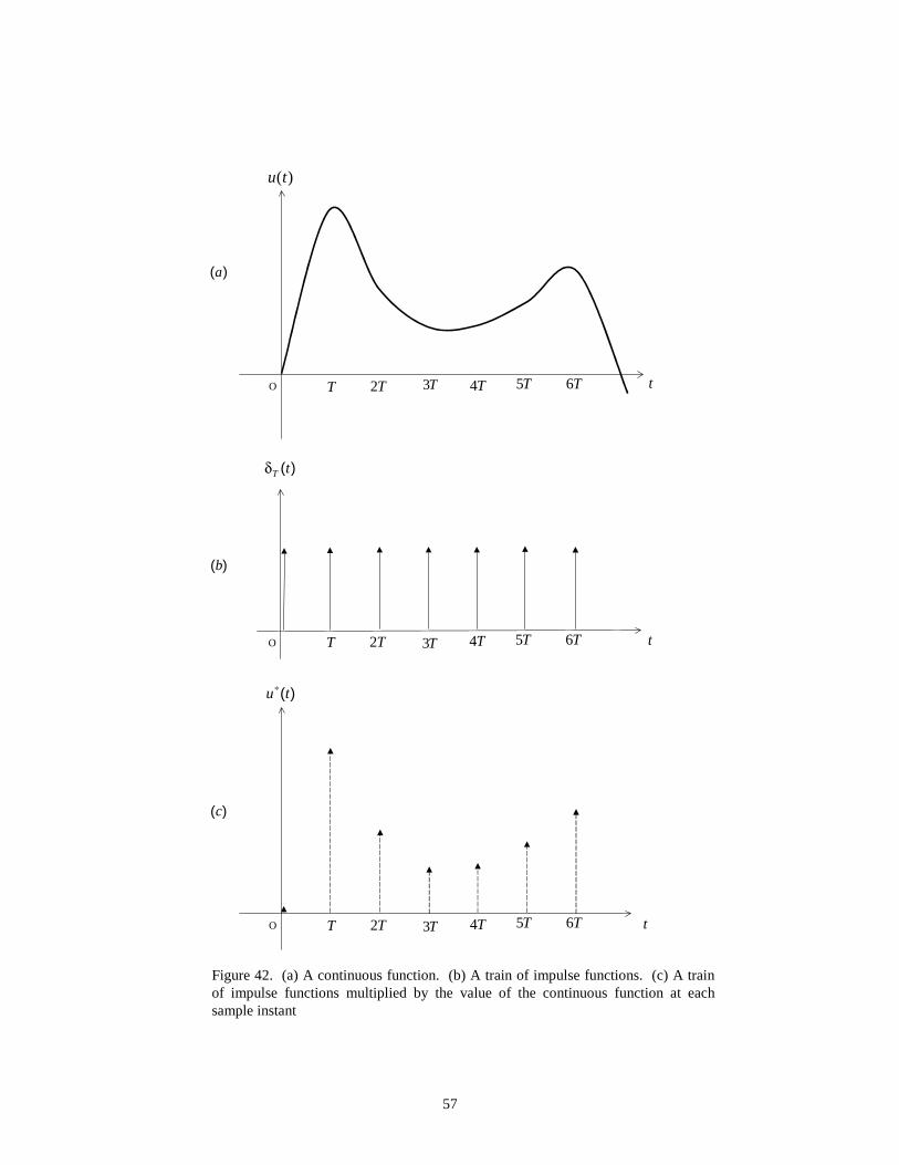
57
Figure 42. (a) A continuous function. (b) A train of impulse functions. (c) A train of impulse functions multiplied by the value of the continuous function at each sample instant
O
)(tu
T T2 T3 T4 T5 T6 t
)(a
O
)(tu∗
T T2 T3 T4 T5 T6 t
)(c
O
)(tTδ
T T2 T3 T4 T5 T6 t
)(b

58
The ideal sampler, represented in figure 41 by a switch, is used to get samples of )U(s at T instants
in time. This time history of impulses or “spikes” have high frequency components and will affect the filter )(s very differently than the original continuous signal. To prevent this distortion, a reconstruction is
made using a polygonal hold block. The polygonal (also called triangular hold) reconstructs the signal and has lower frequency components and much more closely matches the original signal being applied to
)(s . Figure 43 shows how a continuous function )(tu can be approximated using this polygonal hold
technique [Ref. 18].
Figure 43. A polygonal hold piecewise linear approximation to the continuous function )(tu .
The polygonal hold is like the trapezoidal rule of numerical integration. The function being approximated is replaced by piecewise linear chord segments of the curve. The chord slopes can be thought of as being constructed from the sum of pairs of triangular functions.
O
)(tu
time
T T2 T3 T4 T5 T6

59
Figure 44. Details of the two triangular generating functions used to generate a segment of the polygonal hold approximation.
T
Tuttg
)()( += 01
−+=
T
ututg
)()()(
0002
−+=+
T
uTututgtg
)()()()()(
0021
This mathematical construction requires a starting point T− and temporary origin at each sample point. This triangle can be further thought of as being constructed by the superposition of three ramp functions. These ramp functions can be converted into their Laplace transform equivalents more easily than the original construction. This solution is a graphical aid to justify the process. Another method uses a set of infinite series to make this approximation in a more formal mathematical way but is not included here.
T T2
)(tg1
)(tg2
)()( tgtg 21 +
T− 0
)(tu
t
)(tu

60
Figure 45. The triangular hold function as the superposition of simple ramp functions [Ref. 18].
The triangle generating function as a sum of ramp equations is:
)()( TtT
th += 11
tT
th2
2 −=)( (57)
)()( TtT
th −= 13
The Laplace transform of each ramp equation according to the Laplace transform definition is
∫∫∞
−
−∞
−
− +=T
st
T
st dtedtteT
s1
)(1
∫∞
−−=0
2
2)( dtte
Ts st (58)
Tslope
1+=T
1+
T
2−
)(a
)(b
1
T− T+0
T− T+0
1
)(th
)(th1 )(th3
)(th2

61
∫∫∞
−∞
− −=T
st
T
st dtedtteT
s1
)(3 .
Begin the integration at one time step before time zero to permit this construction. This amounts to a modification to the usual definition of integration limits of the Laplace transform. The function being transformed can be restricted to be zero during the one negative step to prevent any convergence problems. It can also be looked at as an approximation that neglects only one step and will be very similar to the result if the integration limit started at zero. Change the integration limit to allow one integral term to be split in two. This technique is used to make the integration limits of several terms match so that they can be algebraically added and canceled.
∫∫∫∞
−
−
−∞
− ++=T
stT
T
st
T
st dtedteT
dtteT
t11
)(1
∫∫ −∞
− −−=T
st
T
st dtteT
dtteT
t0
2
22)( (59)
∫∫∞
−∞
− −=T
st
T
st dtedtteT
t1
)(3
Add the Laplace transform of each of the three ramp functions together.
)()()()( 321 ssss ++=∆
The first term of each of the component functions when added cancel to zero, and the last term of )(1 s and )(3 s cancel. The remaining terms sum to
∫∫∫ −
−
−
−
−∆ −+=
Tst
T
T
stT
T
st dtteT
dtedtteT
s0
21)( . (60)
Use integration by parts on the first and last term.
Tstst
T
T
stT
T
stst
s
e
s
et
Ts
e
s
e
s
et
Ts
0
22
21)(
++
−
+−=
−−
−
−
−
−−
∆
Factor the result to get the expression in [Ref. 18].
TsTs eTsTs
eTs
s −∆ +−= 222
121)( . (61)
Multiply this expression by TsTsee − and regroup to factor and obtain the expression for the triangular hold transfer function in [Ref. 9].

62
2
2)1()(Tsees
TsTs −+
∆−= (62)
The digitally sampled equivalent of )(s is )(z .
[ ])()()( ssz ∆= (63)
Likewise )(s is replaced by )(z , and )(s by )(z .
Figure 46. Z-transform equivalent of a continuous linear system.
Figure 47. Z-transform version of the shaping filters showing the component Laplace transform expressions and the sampling function.
gu
gv
gw
noiseu
noisev
noisew
coeffu
coeffv
coeffw
β+∆us
1HZ
β+α+
∆v
v
ss
HZ
Lag
Lag Lead
β+∆vs
1HZ
β+∆ws
1HZ
β+α+
∆w
w
ss
HZ
[ ])G()(H ss∆Z )(zY
)(zG
)(zU
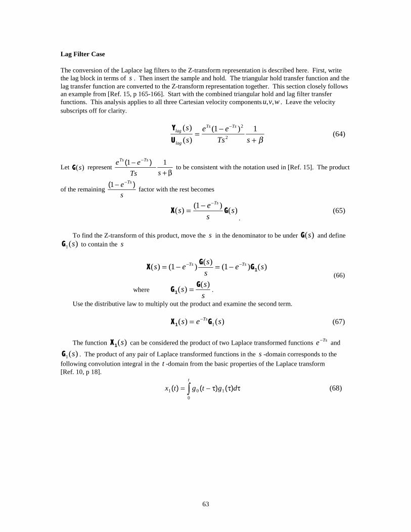
63
Lag Filter Case
The conversion of the Laplace lag filters to the Z-transform representation is described here. First, write the lag block in terms of s . Then insert the sample and hold. The triangular hold transfer function and the lag transfer function are converted to the Z-transform representation together. This section closely follows an example from [Ref. 15, p 165-166]. Start with the combined triangular hold and lag filter transfer functions. This analysis applies to all three Cartesian velocity components wvu ,, . Leave the velocity subscripts off for clarity.
β+−=
−
sTs
ee
s
s TsTs
lag
lag 1)1(
)(
)(2
2
(64)
Let )(s represent β+
− −
sTs
ee TsTs 11 )( to be consistent with the notation used in [Ref. 15]. The product
of the remaining s
e Ts )( −−1 factor with the rest becomes
)()1(
)( ss
es
Ts
−−=
. (65)
To find the Z-transform of this product, move the s in the denominator to be under )(s and define )(1 s to contain the s
)()1()(
)1()( ses
ses TsTs
1
−− −=−= (66)
where s
ss
)()(
=1 .
Use the distributive law to multiply out the product and examine the second term.
)()( 1 ses Ts −=1 (67)
The function )(s1 can be considered the product of two Laplace transformed functions Tse− and
)(1 s . The product of any pair of Laplace transformed functions in the s -domain corresponds to the
following convolution integral in the t -domain from the basic properties of the Laplace transform [Ref. 10, p 18].
∫ τττ−=t
dgtgtx0
101 )()()( (68)
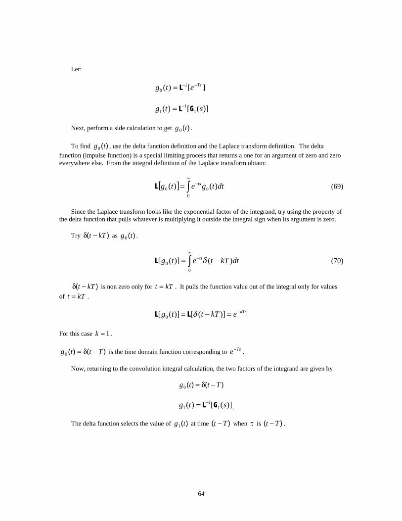
64
Let:
][)( 10
Tsetg −−=
)]([)( 11
1 stg −=
Next, perform a side calculation to get )(tg0 .
To find )(tg0 , use the delta function definition and the Laplace transform definition. The delta
function (impulse function) is a special limiting process that returns a one for an argument of zero and zero everywhere else. From the integral definition of the Laplace transform obtain:
[ ] ∫∞
−=0
00 )()( dttgetg ts (69)
Since the Laplace transform looks like the exponential factor of the integrand, try using the property of the delta function that pulls whatever is multiplying it outside the integral sign when its argument is zero.
Try )( kTt −δ as )(tg0 .
∫∞
− −=0
0 )()]([ dtkTtetg tsδ (70)
)( kTt −δ is non zero only for kTt = . It pulls the function value out of the integral only for values
of kTt = .
kTsekTttg −=−= )]([)]([ 0 δ
For this case 1=k .
)()( Tttg −δ=0 is the time domain function corresponding to Tse− .
Now, returning to the convolution integral calculation, the two factors of the integrand are given by
)()( Tttg −δ=0
)]([)( 11
1 stg −= .
The delta function selects the value of )(tg1 at time )( Tt − when τ is )( Tt − .

65
∫ τττ−−δ=t
dgTttx0
11 )()()(
)()( Ttgtx −= 11
Take the Z-transform of both sides:
)]([)]([ 11 Ttgtx −=
Define the Z-transform of the function )(tg1 to be
)]([)( 11 tgz = . (71)
From the Z-transform real translation theorem (shifting theorem), [Ref. 15, p 52], the Z-transform of )(tg1 is
)()]([)]([ )( 11
111 zzTtgtxz −=−== . (72)
From equation (66),
)()1()( ses Ts1 −−=
taking the Z-transform of both sides we get
)]()1[()]([ ses Ts1 −−=
)]()([)( sesz Ts11 −−= .
Replace the Z-transform from the s -domain of the first term with the corresponding Z-transform from the t -domain.
)]([ )]([)( 11 setgz Ts −−= (73)
Use equation (67) to substitute for the second term.
[ ] [ ])()()( 11 stgz −=
)()()( 11 zzz −= (74)
Use equation (72) to substitute in place of the second term of equation (74) and factor common terms.

66
)()()( 11
1 zzzz −−=
)()1()( 11 zzz −−= (75)
To summarize this process, if )(s involves a factor )( Tse −−1 , then to obtain the Z-transform of
)(s , the term )( Tse −−1 may be factored out so that )(z becomes the product of )( 11 −− z and the
Z-transform of the remaining term. As a check, remember that from the definition of z from sampled
control theory, sTez = [Ref. 15, p 150]. Make this substitution to verify the correspondence between
)( Tse −−1 and )( 11 −− z .
−== −
s
szsz
)()1()]([)( 1 (76)
Substitute back in for s
s)( and repeat the process to get the Z-transform of the second )( Tse −−1
factor. Take the Z-transform of the second )( Tse −−1 factor and the rest:
+−− −−
)(
1)1()1(
21
βsTseez TsTs
In like manner to the process that pulled out the )( 11 −− z factor, the )( Tse −−1 factor is pulled out of
the Z-transform operator.
+
−−= −−
)(
1)1)(1()(
2
11
βsTsezzz Ts (77)
Consider the remaining Z-transformed product:
+ )(
12 βsTs
eTs
Again, let )(s be redefined to represent )(
1
β+sTs with
s
ss
)()(1
= .
Redefine )(1 s to be the product of the two Laplace transformed functions Tse and )(1 s .
)()( 11 ses Ts = (78)
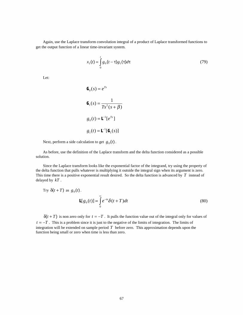
67
Again, use the Laplace transform convolution integral of a product of Laplace transformed functions to get the output function of a linear time-invariant system.
∫ τττ−=t
dgtgtx0
101 )()()( (79)
Let:
Tses =)(0
)(
1)(
21 β+=
sTss
][)( 10
Tsetg −=
)]([)( 11
1 stg −=
Next, perform a side calculation to get )(tg0 .
As before, use the definition of the Laplace transform and the delta function considered as a possible
solution. Since the Laplace transform looks like the exponential factor of the integrand, try using the property of
the delta function that pulls whatever is multiplying it outside the integral sign when its argument is zero. This time there is a positive exponential result desired. So the delta function is advanced by T instead of delayed by kT .
Try )( Tt +δ as )(tg0 .
∫∞
− +=0
0 )()]([ dtTtetg tsδ (80)
)( Tt +δ is non zero only for Tt −= . It pulls the function value out of the integral only for values of
Tt −= . This is a problem since it is just to the negative of the limits of integration. The limits of integration will be extended on sample period T before zero. This approximation depends upon the function being small or zero when time is less than zero.
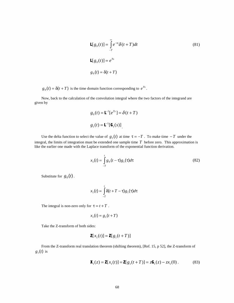
68
∫∞
−
− +=T
ts dtTtetg )()]([ 0 δ (81)
Tsetg =)]([ 0
)()( Tttg +δ=0
)()( Tttg +δ=0 is the time domain function corresponding to Tse .
Now, back to the calculation of the convolution integral where the two factors of the integrand are
given by
)(][)( 10 Ttetg Ts +== − δ
)]([)( 11
1 stg −= .
Use the delta function to select the value of )(tg1 at time T−=τ . To make time T− under the
integral, the limits of integration must be extended one sample time T before zero. This approximation is like the earlier one made with the Laplace transform of the exponential function derivation.
∫−
τττ−=t
T
dgtgtx )()()( 101 (82)
Substitute for )(tg0 .
∫−
τττ−+δ=t
T
dgTttx )()()( 11
The integral is non-zero only for Tt +=τ .
)()( Ttgtx += 11
Take the Z-transform of both sides:
)]([)]([ 11 Ttgtx +=
From the Z-transform real translation theorem (shifting theorem), [Ref. 15, p 52], the Z-transform of )(tg1 is
)0()()]([)]([)( 11111 zxzzTtgtxz −=+== . (83)
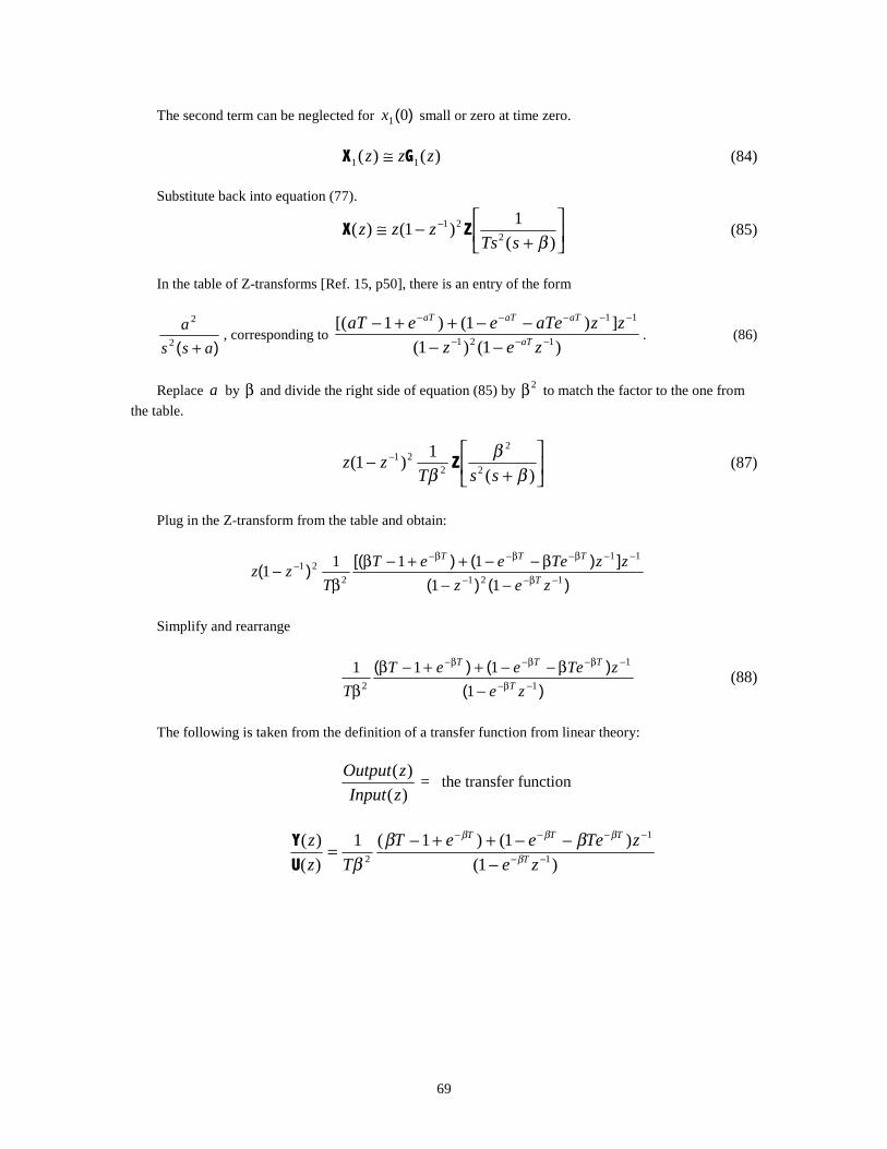
69
The second term can be neglected for )(01x small or zero at time zero.
)()( 11 zzz ≅ (84)
Substitute back into equation (77).
+−≅ −
)(
1)1()(
221
βsTszzz (85)
In the table of Z-transforms [Ref. 15, p50], there is an entry of the form
)( ass
a
+2
2
, corresponding to )1()1(
])1()1[(121
11
−−−
−−−−−
−−−−++−
zez
zzaTeeeaTaT
aTaTaT
. (86)
Replace a by β and divide the right side of equation (85) by 2β to match the factor to the one from
the table.
+
− −
)(
1)1( 2
2
221
ββ
β ssTzz (87)
Plug in the Z-transform from the table and obtain:
)()(
])()[()(
121
11
221
11
1111
−β−−
−−β−β−β−−
−−β−−++−β
β−
zez
zzTeeeT
Tzz
T
TTT
Simplify and rearrange
)(
)()(1
1
2 1
111−β−
−β−β−β−
−β−−++−β
β ze
zTeeeT
T T
TTT
(88)
The following is taken from the definition of a transfer function from linear theory:
)(
)(
zInput
zOutput = the transfer function
)1(
)1()1(1
)(
)(1
1
2 −−
−−−−
−−−++−=
ze
zTeeeT
Tz
zT
TTT
β
βββ βββ
70
Arrange terms using algebra:
)()1(1
)()1(1
)1)(( 122
1 zzTeeT
zeTT
zez TTTT −−−−−− −−++−=− ββββ ββ
ββ
)()1(1
)()1(1
)()(2
12
1 zeTT
zzTeeT
zzez TTTT ββββ ββ
ββ
−−−−−− +−+−−+= (89)
The real translation theorem (shifting theorem) of the Z-transform from [Ref. 15, p 52]:
If 0=)(tx for 0<t and )(tx has the z transform )(z , then )()( zznTtx n−=−
where n is zero or a positive integer.
For the case where n is 0,
)()( ztx = .
For the case where n is 1,
)()( 1 zzTtx −=− .
Consider only the instants of time when sample frames are taken kT where k is the frame number:
)(z is replaced by )(kT ,
)(1 zz − is replaced by )( TkT − ,
)(1 zz − is replaced by )( TkT − ,
)(z is replaced by )(kT .
[ ] )(11
)()(2 TkTTee
TTkTekT TTT −−−+−= −−− βββ β
β
[ ] )(11
2 kTeTT
T
βββ
−+−+ (90)
71
Define the coefficient symbols:
L
V0=β
−β
−β
= )( DT
A 11
11
(91)
)( DAB −β
+−= 11
TeD β−=
Perform the algebraic manipulation and the difference equation for the lag filter in order to derive the form found in the gust model code. [Ref. 9]
First order time lag as a function of time is:
][])1[(])1[(][ kTATkBTkDkT laglag ⋅+−⋅+−⋅= (92)
First order time lag as a function of z is:
)()()()( 11 zAzBzDz laglag ⋅+⋅+⋅= −− (93)
72
Lag Lead Filter Case
The conversion of the Laplace lag lead filters to the Z-transform representation follows the lag filter case of the previous section. As before, write the lag lead block in terms of s . Then insert the sample and hold. The triangular hold transfer function and the lag lead transfer function are converted to the Z-transform representation together. Start with the combined triangular hold and lag lead transfer functions. This analysis applies to the velocity components v and w that are not in the longitudinal motion direction. The subscripts can be left off for clarity.
βα
++−=
−
s
s
Ts
ee
s
s TsTs
leadlag
leadlag
2
2
_
_ )1(
)(
)(
(94)
Let )(s represent β+α+− −
s
s
Ts
ee TsTs
2
1 )( . The product of the remaining )( Tse −−1 factor with the
rest becomes
)()1()( ses Ts −−=. (95)
To summarize this process, if )(s involves a factor )( Tse −−1 , then to obtain the Z-transform of
)(s , the term )( Tse −−1 may be factored out so that )(z becomes the product of )( 11 −− z and the Z-
transform of the remaining term. As a check, remember that from the definition of z from sampled control
theory, sTez = , [Ref. 15, p 150]. Make this substitution to verify the correspondence between
)( Tse −−1 and )( 11 −− z .
[ ])()1()]([)( 1 szsz −−== (96)
Substitute back in for )(s and repeat the process to get the Z-transform of the second )( Tse −−1
factor. Take the Z-transform of the second )( Tse −−1 factor and the rest:
++−− −−
)()1()1(
21
βα
sTs
seez TsTs
In like manner to the process that pulled out the )( 11 −− z factor, the )( Tse −−1 factor is pulled out of
the Z-transform operator.
++−− −−
)()1)(1(
211
βα
sTs
sezz Ts (97)
Tse can be pulled out and converted to z . See the two pages preceding the equation (85) result in the section on the lag filter case for the details.

73
++− −
)(
1)1(
221
βα
ss
s
Tzz
++
+− −
)()(
11)1(
221
βα
β ssssTzz (98)
In the table of z transforms from [Ref. 15, p 50], there is an entry of the form
)( ass
a
+, (99)
and also an entry of the form
)(2
2
ass
a
+. (100)
Manipulate constants to get the table factor form
+
++
− −
)()(
11)1(
2
2
221
ββ
βα
ββ
β ssssTzz , (101)
and plug in the Z-transform from the table to get
−−
β−−++−ββα+
−−−
β−
−β−−
−−β−β−β−
−β−−
−β−−
)()(
])()[(
))((
)()(
121
11
211
121
11
11
11
1111
zez
zzTeeeT
zez
ze
Tzz
T
TTT
T
T
.
Simplify and rearrange.
−−
β−−++−ββα+
−−
β−
−β−−
−β−β−β−
−β−
β−−
))((
])()[(
)(
)()(
11
1
211
11
11
1
1111
zez
zTeeeT
ze
e
Tz
T
TTT
T
T
−
β−−++−βα+−−ββ −β−
−β−β−β−β−−
1
11
2 1
11111
ze
zTeeeTez
T T
TTTT ])()[())((. (102)
The following is taken from the definition of transfer function:
)(
)(
zInput
zOutput = the transfer function

74
−
−−++−+−−= −−
−−−−−−
1
11
2 1
])1()1[()1)(1(1
)(
)(
ze
zTeeeTez
Tz
zT
TTTT
β
ββββ ββαββ
.
Arrange terms using algebra.
[ ] )()1(1()1(1
)1)(( 12
1 zzeeTeeT
zez TTTTT
−−−−−−− −−−+−−=− βββββ ββαβ
[ ] )()1(1
2 zeTT
T ββαβ
−−−+
)()1(1
)()( 12
1 zzTeeT
zzez TTT −−−−− −−+= βββ βαβ
)()]1([1
2 zeTT
T ββαβ
−−−+ (103)
Using the shifting theorem of the Z-transform,
)(z is replaced by )(kT ,
)(1 zz − is replaced by )( TkT − ,
)(1 zz − is replaced by )( TkT − ,
)(z is replaced by )(kT , and
])1[()1(])1[()( 2 TkTeeT
TkekT TTT −−−+−= −−−
βββ ββα
)()1(2 kTeTT
T
βββα −+−+ (104)
where k is the frame number.
75
Define the coefficient symbols:
L
V0=β
−
β−
β= )( D
TA 1
11
1
TeD β−= (105)
)( DT
I −
β
−+= 13
11
3
1
)( DIJ −βα+−= 1
Perform the algebraic manipulation and the difference equation for the lag filter in order to derive the form found in [Ref. 9] and the gust model code.
First order lag lead as a function of time is:
][])1[(])1[(][ __ kTITkJTkDkT leadlagleadlag ⋅+−⋅+−⋅= (106)
First order lag lead as a function of z is:
)()()()( 11__ zIzJzDz leadlagleadlag ⋅+⋅+⋅= −− (107)

76
Random Number Generator
Figure 48. Uniform random numbers modified to produce Gaussian white noise.
A portable uniform random number generator is selected from [Ref. 17, p 283] originally written by D. Knuth. This replaces the random number generator used in the Airlab simulation, RANFP, which was found to have problems. Airlab did not have a great need for gust response and the random number generator was not given much attention when the software was converted from the CDC NOS machine to the VAX 750. Periodicity in some observed control parameters pointed to a problem with the Dryden gust model. The periodicity was traced to the random number generator RANFP. A plot of a 400 number sequence of random numbers produced by RANFP followed by 400 numbers from the D. Knuth generator “ran3Knuth” is shown for comparison.
Knuth UniformRandom NumberGenerator
Gaussian RandomNumberTransformation
Gaussian WhiteNoise to driveDryden ShapingFilters
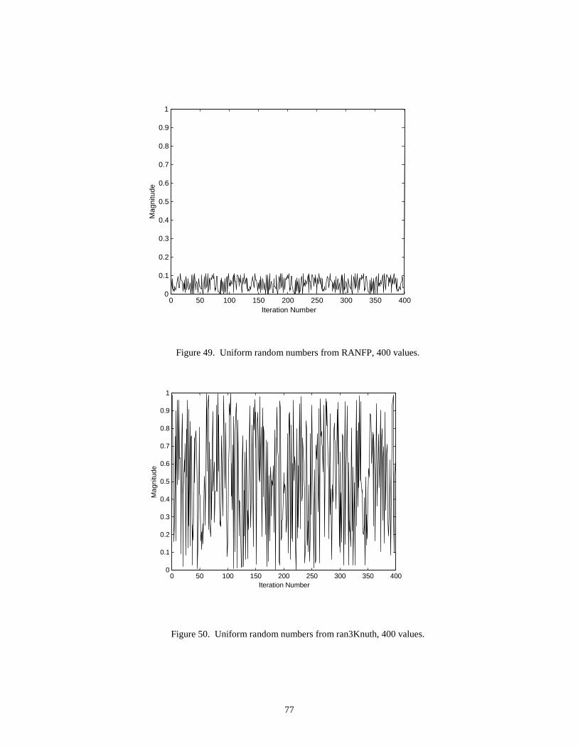
77
Figure 49. Uniform random numbers from RANFP, 400 values.
Figure 50. Uniform random numbers from ran3Knuth, 400 values.
0 50 100 150 200 250 300 350 4000
0.1
0.2
0.3
0.4
0.5
0.6
0.7
0.8
0.9
1
Iteration Number
Mag
nitu
de
0 50 100 150 200 250 300 350 4000
0.1
0.2
0.3
0.4
0.5
0.6
0.7
0.8
0.9
1
Iteration Number
Mag
nitu
de

78
Except for an unexplained factor of 10 scale decrease, the RANFP doesn’t look too bad at first glance. However, if the first 200 numbers are paired with the second 200 numbers and plotted as an (x,y) coordinate pair, the following non-random behavior is produced by RANFP. Notice that figure 51 and 52 do not have the same scale.
Figure 51. Pairs of uniform random numbers from RANFP.
Figure 52. Pairs of uniform random numbers from ran3Knuth.
0 0.05 0.1 0.15 0.20
0.02
0.04
0.06
0.08
0.1
0.12
0.14
0.16
0.18
0.2
x Magnitude
y M
agni
tude
0 0.2 0.4 0.6 0.8 10
0.1
0.2
0.3
0.4
0.5
0.6
0.7
0.8
0.9
1
x Magnitude
y M
agni
tude

79
The Knuth generator, ran3Knuth, based on ran3 from [Ref. 17, p 282], is designed to be portable across different computer systems. This implementation has been verified to work with Sun FORTRAN, and Sun as well as Windows95 PC C, and Simulink, and C code generated from Simulink Real-Time Workshop.
Figure 53. A 50 bin histogram of 10000 Gaussian distributed random numbers from gasdev.
The uniform random numbers need to be modified to generate the required Gaussian distributed white noise for the Dryden gust model. The Box-Muller transformation method is used to generate a Gaussian random number from a uniform random number. Subroutine “gasdev” from [Ref. 17, p 289] is used to generate Gaussian random numbers in the B-737 Linear Autoland Simulink Model. Figure 53 shows the expected bell-shaped curve Gaussian character of the numbers generated. Figure 54 is a plot of pairs of the Gaussian random numbers and is evidence of the lack of unwanted periodicity.
-5 -4 -3 -2 -1 0 1 2 3 40
100
200
300
400
500
600
70050 Bin Histogram of 10,000 Calls to gasdev
gasdev output value
Num
ber
of O
ccur
ance
s
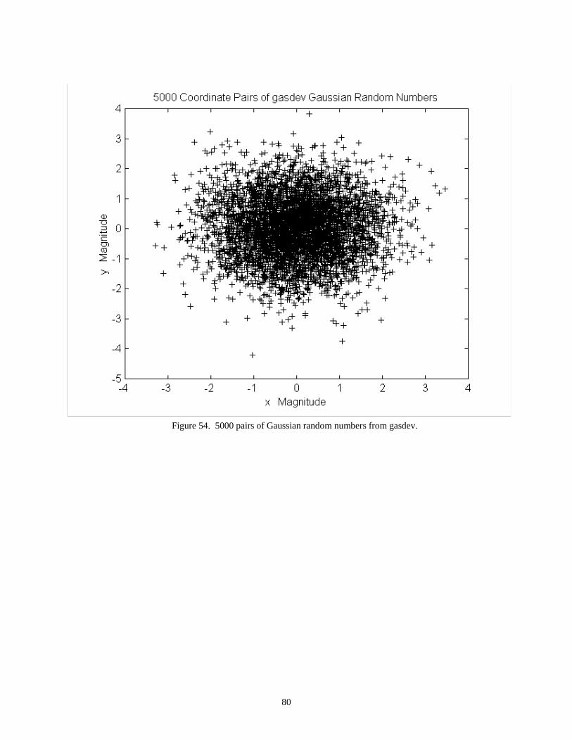
80
Figure 54. 5000 pairs of Gaussian random numbers from gasdev.

81
Autopilot Control Concepts
Figure 55. Basic control terminology adapted from chapter 2 [DiStefano III].
• Control Set Point
A controller and a plant use feedback to maintain a desired state of the system. The desired state of the system is fed in through an input and compared with the present state of the system in a summing junction. The difference in the two values is the error signal. This error signal is sent to the controller which calculates the “manipulated variables” so as to move the plant closer to the desired set point. The state of the system is sent back to be compared with the input and is output as the new state of the system. This completes the “feedback” loop.
• Control Error
“Error” used in the feedback control context means the difference between the commanded and preexisting state of the system. It is not used in the sense of being a mistake or system defect. The controller attempts to minimize this error signal.
rudder
aileron
elevator
throttle
(Airplane)(Autopilot)Actual Airplane
Heading
ManipulatedVariables
Controller PlantControlled
Output
ReferenceInput
PrimaryFeedback
r
b
e
Error
−
+
AutopilotSet-Point
c
u
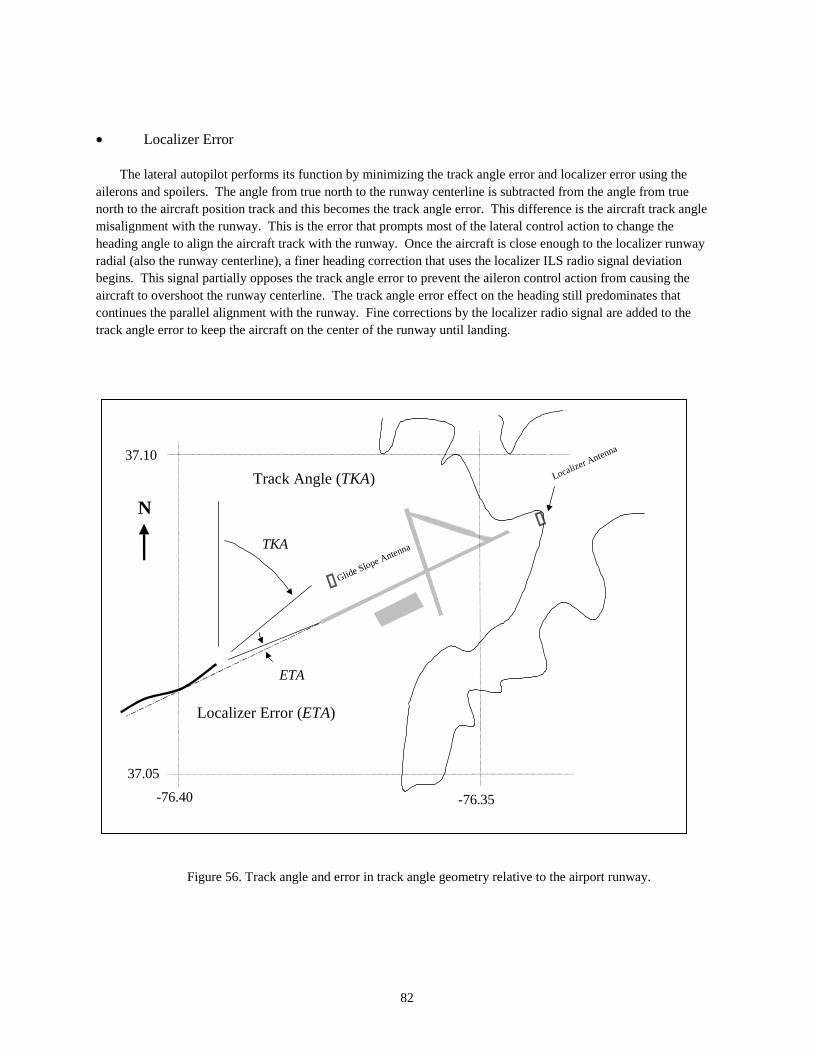
82
• Localizer Error
The lateral autopilot performs its function by minimizing the track angle error and localizer error using the ailerons and spoilers. The angle from true north to the runway centerline is subtracted from the angle from true north to the aircraft position track and this becomes the track angle error. This difference is the aircraft track angle misalignment with the runway. This is the error that prompts most of the lateral control action to change the heading angle to align the aircraft track with the runway. Once the aircraft is close enough to the localizer runway radial (also the runway centerline), a finer heading correction that uses the localizer ILS radio signal deviation begins. This signal partially opposes the track angle error to prevent the aileron control action from causing the aircraft to overshoot the runway centerline. The track angle error effect on the heading still predominates that continues the parallel alignment with the runway. Fine corrections by the localizer radio signal are added to the track angle error to keep the aircraft on the center of the runway until landing.
Figure 56. Track angle and error in track angle geometry relative to the airport runway.
-76.40 -76.35
37.05
37.10
Localizer Antenna
Glide Slope Antenna
N
Localizer Error (ETA)
ETA
Track Angle (TKA)
TKA
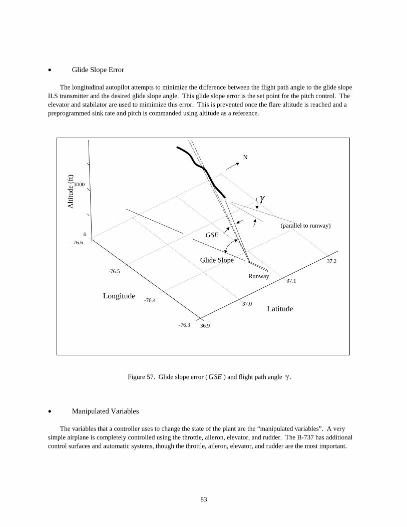
83
• Glide Slope Error
The longitudinal autopilot attempts to minimize the difference between the flight path angle to the glide slope ILS transmitter and the desired glide slope angle. This glide slope error is the set point for the pitch control. The elevator and stabilator are used to mimimize this error. This is prevented once the flare altitude is reached and a preprogrammed sink rate and pitch is commanded using altitude as a reference.
Figure 57. Glide slope error ( GSE ) and flight path angle γ .
• Manipulated Variables
The variables that a controller uses to change the state of the plant are the “manipulated variables”. A very simple airplane is completely controlled using the throttle, aileron, elevator, and rudder. The B-737 has additional control surfaces and automatic systems, though the throttle, aileron, elevator, and rudder are the most important.
0
Alti
tude
(ft
)
1000
-76.5
-76.4
36.9
37.1
Latitude
Longitude37.0
37.2
-76.6
-76.3
N
Glide Slope
GSE
γ
(parallel to runway)
Runway
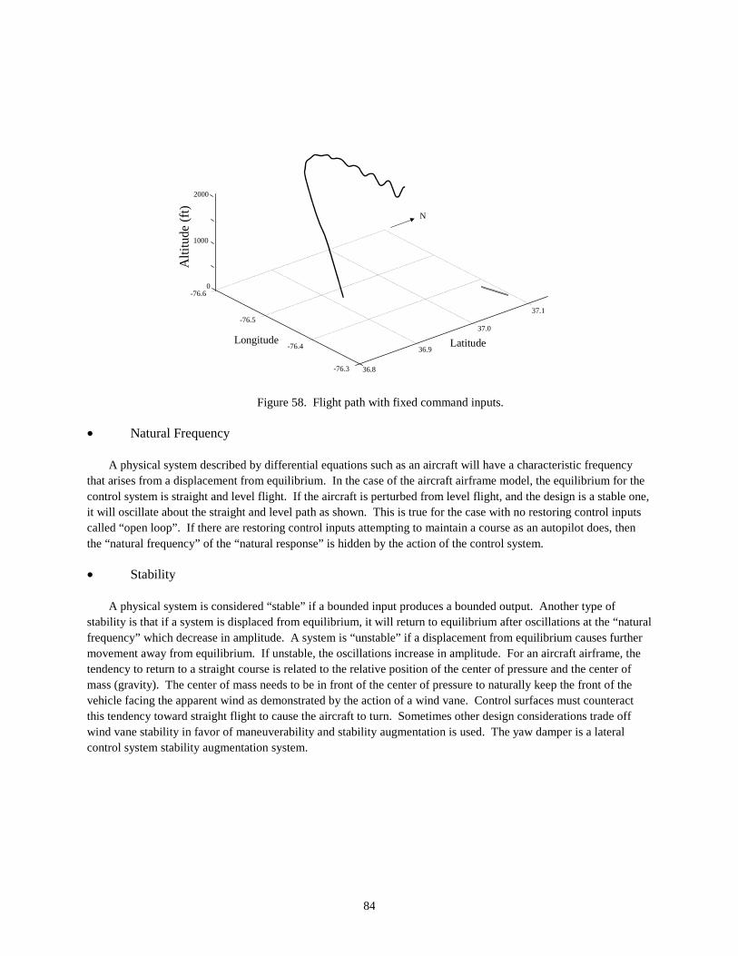
84
Figure 58. Flight path with fixed command inputs.
• Natural Frequency
A physical system described by differential equations such as an aircraft will have a characteristic frequency that arises from a displacement from equilibrium. In the case of the aircraft airframe model, the equilibrium for the control system is straight and level flight. If the aircraft is perturbed from level flight, and the design is a stable one, it will oscillate about the straight and level path as shown. This is true for the case with no restoring control inputs called “open loop”. If there are restoring control inputs attempting to maintain a course as an autopilot does, then the “natural frequency” of the “natural response” is hidden by the action of the control system.
• Stability
A physical system is considered “stable” if a bounded input produces a bounded output. Another type of stability is that if a system is displaced from equilibrium, it will return to equilibrium after oscillations at the “natural frequency” which decrease in amplitude. A system is “unstable” if a displacement from equilibrium causes further movement away from equilibrium. If unstable, the oscillations increase in amplitude. For an aircraft airframe, the tendency to return to a straight course is related to the relative position of the center of pressure and the center of mass (gravity). The center of mass needs to be in front of the center of pressure to naturally keep the front of the vehicle facing the apparent wind as demonstrated by the action of a wind vane. Control surfaces must counteract this tendency toward straight flight to cause the aircraft to turn. Sometimes other design considerations trade off wind vane stability in favor of maneuverability and stability augmentation is used. The yaw damper is a lateral control system stability augmentation system.
0
Alti
tude
(ft
)2000
1000
-76.5
-76.4
36.8
37.0
LatitudeLongitude36.9
37.1
-76.6
-76.3
N

85
• Symmetry
The symmetry of the typical airplane allows separation of the control of the longitudinal motion from the control of the lateral motion [Ref. 20, p 48]. The symmetry reduces every rolling torque and side force to zero. This approximation still is good for small turns and sideslips. The B-737 autopilot makes this approximation and separates the longitudinal control system from the lateral control system.
• Rate Control
The aileron is a rate control device. The angular velocity of the roll is proportional to the angular deflection of the aileron control wheel. As long as the control wheel is deflected, the airplane will roll with a constant angular rate.
• Position Control
The elevator is a position control device. The angle of pitch is proportional to the yoke deflection. When the yoke is deflected, the airplane will orient to the new pitch orientation and remain there. The pitch angle will not keep changing for a constant yoke deflection.
Autothrottle
Figure 59. Autothrottle feedback loop.
The autothrottle keeps the airspeed the same until flare, then it decreases. The elevator is used to keep the airplane on the glide slope, and the autothrottle does what is necessary to keep the calibrated airspeed )(CAS the same coming down the glide slope.
throttleAirplaneThrottle
Autopilot
ActualAirplane CAS
ManipulatedVariable
CASFeedback
r
b
e−
+
CAS atStart ofLanding
c
CAS ErrorUntil Flare
u
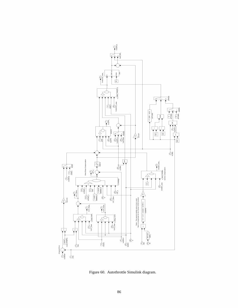
86
Figure 60. Autothrottle Simulink diagram.
vers
ine
com
pens
atio
n
Win
d S
hear
Com
pens
atio
n
Airs
peed
Err
or
*Not
e: T
he s
peci
al m
atla
b va
lue
of p
i is
used
here
to c
om
pens
ate
for
the
For
tran
CO
SD
func
tion.
8
TH
RO
TLE
_sta
te_
7
DLE
PR
_
6
CA
SB
K_s
tate
_
5
V2F
_y_
4
V2F
_upa
st_
3
V1F
2_st
ate_
2
V1F
1_st
ate_
1
TH
RO
TLE
in LOW
HIG
H
out
xlim
switc
h3
s_w
out_
V1F
1
s_w
out_
CA
SB
K
s_m
odla
g1
s_fo
lag_
V1F
2
s_eu
lint_
TH
RO
TLE
0
hold
_F
flare
_tes
t_
60.
200.
250.
250.
16.
apcp
rm
XN
CL1
0
XD
DC
1X
DD
C
TH
DU
M
.2
TA
UK
4
><
>=
+0.
2
RT
GK
5_2
-0.2
RT
GK
5_1
OR
AN
D
OR
16.
1.2
GK
VD
T
0.1
GK
CA
S
0.2
GK
5
180.
/u[1
]
DP
R_
1.6
878
Cns
t_K
TO
FP
S
5.0
* (
1.0
- co
s(u[
1] *
pi/1
80.)
)
CA
SP
HI
+1.
0e3
5
AM
GK
5_2
-1.0
e35
AM
GK
5_1
.2 *
(25
0. -
u[1
])
AF
TLI
M3
0.
AF
TLI
M2
10.
AF
TLI
M1
AF
TLI
M
23
TH
RO
TLE
_sta
te
22
DLE
PR
21
CA
SB
K_s
tate
20
V2F
_y
19
V2F
_upa
st18
V1F
2_st
ate
17
V1F
1_st
ate
16
TH
RT
RIM
15 h
14 PI
13 T
12
RE
SE
T
11
TH
RO
TLC
10
CLA
MP
9
SQ
UIS
H
8
FLA
RE
7
EP
R
6
PH
I
5
VG
SD
OT
4
TA
S
3
CA
SE
NG
2
CA
SM
SP
1
CA
S
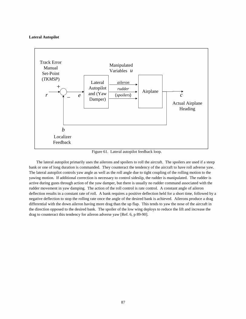
87
Lateral Autopilot
Figure 61. Lateral autopilot feedback loop.
The lateral autopilot primarily uses the ailerons and spoilers to roll the aircraft. The spoilers are used if a steep bank or one of long duration is commanded. They counteract the tendency of the aircraft to have roll adverse yaw. The lateral autopilot controls yaw angle as well as the roll angle due to tight coupling of the rolling motion to the yawing motion. If additional correction is necessary to control sideslip, the rudder is manipulated. The rudder is active during gusts through action of the yaw damper, but there is usually no rudder command associated with the rudder movement in yaw damping. The action of the roll control is rate control. A constant angle of aileron deflection results in a constant rate of roll. A bank requires a positive deflection held for a short time, followed by a negative deflection to stop the rolling rate once the angle of the desired bank is achieved. Ailerons produce a drag differential with the down aileron having more drag than the up flap. This tends to yaw the nose of the aircraft in the direction opposed to the desired bank. The spoiler of the low wing deploys to reduce the lift and increase the drag to counteract this tendency for aileron adverse yaw [Ref. 6, p 89-90].
)(spoilers
rudder
aileron
Airplane
LateralAutopilotand (YawDamper)
Actual AirplaneHeading
ManipulatedVariables
LocalizerFeedback
r
b
e−
+
Track ErrorManual
Set-Point(TKMSP)
c
u

88
Lateral Autopilot Simulink Diagram
Figure 62. Lateral autopilot Simulink diagram.
25
PH
ICM
D_s
tate
_
24
LOC
CF
_sta
te_
23
XT
KD
MP
_sta
te_
22
RIN
T5_
21
RIN
T5_
stat
e_
20
DE
CR
AB
_
19
YA
WIN
T_s
tate
_
18
YF
I_st
ate_
17
PS
ILM
P_k
ount
_
16
PS
ILM
P_o
ut_
15
PS
IDZ
_
14
DE
LPS
I_
13
RC
CM
D_k
ount
_
12
RC
CM
D_o
ut_
11
fola
g_st
ate_
10
wou
t_st
ate_
9
PH
IER
R
8
PH
DO
T_
7
AIL
XF
D
6
PH
ICM
D
5
LOC
CM
D_4
LOC
E_
3
ON
CR
S_
2
DE
LRC
1
DE
LAC
xlim
_RF
3L
xlim
_LO
CV
L
s_w
out
s_fo
lag
rudd
er_c
omm
and
oncr
s_te
st
loca
lizer
_com
man
d
INO
UT
limit_
angl
e_de
g
3.0
2.0
.1
.625
2.3
bank
_com
man
d
aile
ron_
com
man
d
|u|
abs_
LOC
DO
T
XT
VE
L
6e-0
4
VLT
AB
L
1.24
TA
UR
F4
0.12
3
TA
UR
F3
< <<
<
u[1]
/180
.
RP
D
PS
IDE
G
XO
R
AN
DO
R
AN
D
OR
AN
D
OR
2.0
LOC
VL
.027
1
LCD
TM
AX 1.
25e-
3
GP
TA
BL
180.
/u[1
]
DP
R_
DE
LTK
A
|u|
Abs
1
|u|
Abs
42
PH
ICM
D_s
tate
41
LOC
CF
_sta
te
40
XT
KD
MP
_sta
te
39
RIN
T5
38
RIN
T5_
stat
e
37
DE
CR
AB
36
YA
WIN
T_s
tate
35
YF
I_st
ate
34
PS
ILM
P_k
ount
33
PS
ILM
P_o
ut
32
IDE
CR
BP
31
PS
IDZ
30
DE
LPS
I
29
ION
CR
SP
28
PH
ICM
D_
27
RC
CM
D_k
ount
26
RC
CM
D_o
ut
25
ILO
CE
P
24
fola
g_st
ate
23
wou
t_st
ate 22 h 21 P
I
20 PS
IR
19 SP
L
18 SP
R
17 KV
16
PE
DA
LC
15
RLO
UT
14
DE
CR
B
13
FLA
RE
12
PH
IHP
C
11 HR
10
RE
SE
T
9
ET
A8
LAN
DA
RM
7 PS
I
6
PH
IDO
T
5 PH
I
4
LOC
E
3
ON
CR
S 2
VG
S
1 TK

89
Longitudinal Autopilot
Figure 63. Longitudinal autopilot feedback loop.
The longitudinal autopilot controls the pitch orientation of the aircraft. The elevator is the primary pitch control device. A slower acting automatic trim system tries to drive the elevator back to zero by moving the horizontal tail surface to which the elevator is attached. This moving assembly is called the stabilator. The action of the pitch control is position control. The aircraft pitches until equilibrium is reached for a given deflection of the elevator. This acts differently than the aileron roll control. The longitudinal autopilot has two major control modes. Vertical path control (VPC) is used to hold a given altitude during normal flight. Once glide slope is engaged and a final Instrument Landing System (ILS) approach begins, the longitudinal autopilot switches to Autoland mode. The glide slope error is used to close the pitch control loop. The autopilot commands pitch down if the aircraft is coming in too high; pitch up if too low. This continues until the altitude where the flare mode begins is attained. Then, a preprogrammed pitch profile for the flare is commanded.
)(stabilator
elevatorAirplaneLongitudinal
Autopilot
Actual AirplaneGlide Slope
ManipulatedVariables
XCG, YCG,HCG Feedback
r
b
e−
+
Glide SlopeSet-Point
c
Glide SlopeError
u
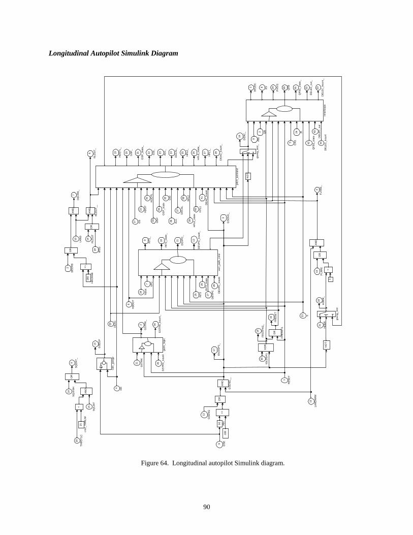
90
Longitudinal Autopilot Simulink Diagram
Figure 64. Longitudinal autopilot Simulink diagram.
34
GS
TR
K_
kou
nt_
33
DE
LEC
_ko
unt
_
32
DE
LEC
_out
_
31
QF
B1_
sta
te_
30 QF
B
29
PH
IVS
28
DE
AC
_kou
nt_
27
HF
L1_
26
HF
L0_
sta
te_
25
HF
L2_
24
DE
CA
L_
23 ALC
_
22 GS
I_
21
GS
P_s
tate
_
20
GS
P_
19
HD
OT
L_
18
HD
ER
_
17
IDLO
GP
1_
16
FR
ST
PA
S_
15
FR
ES
ET
14
DE
AC
_
13
GS
EG
P
12
DE
VP
C_
kou
nt_
11
DE
VP
C_
10
INT
2_st
ate_
9
INT
2_
8 KV
7
DE
CR
B_
6
RLO
UT
_
5
SQ
UA
T_
4
FLA
RE
_
3
GS
EN
G_
2
GS
TR
K_
1
DE
LEC
vert
_pa
th_
cmd
pitc
h_au
tola
nd
OR
inne
rlo
ops
gstr
k_l
ogic
gse
ng_t
est_
gse
ng_t
est
.108
0
15
cns
t_T
HR
LIM
calc
_gse
gp
<=
<=
<
<
AN
D
RLO
UT
__
AN
D
OR
NO
T
OR
AN
D
NO
T
OR
OR
150
.
HR
CR
AB
AN
D
GS
EN
G__
XO
R
OR
FR
ES
ET
1
AN
D
|u|
Abs
45
GS
TR
K_
kou
nt
44
DE
LEC
_ko
unt
43
DE
LEC
_out
42
QF
B1_
sta
te
41
DE
AC
_ko
unt
40
HF
L1
39
HF
L0_
sta
te
38
HF
L2
37
DE
CA
L
36 ALC
35 GS
I
34
GS
P_s
tate
33 GS
P
32
HD
OT
L
31
HD
ER
30
IDLO
GP
1
29
DE
AC
28
DE
VP
C_
kou
nt
27
DE
VP
C
26
INT
2_st
ate
25 INT
2
24 PI
23 h
22
HD
OT
21
GS
TR
K
20
TH
RO
TLC
19
RLO
UT
18
WS
U
17 GS
16
TB
AX
15
SQ
UA
T
14
SQ
UIS
H
13
FLA
RE
12
GS
EN
G
11
LAN
DA
RM
10
LAN
D
9
GS
E
8
PH
I
7
VP
C
6
HD
DO
T
5
CA
S
4
HR
3 QB
2
DE
CR
B
1
RE
SE
T

91
Vertical Path Control
Figure 65. Longitudinal autopilot vertical path control law Simulink diagram.
DE
VP
C
5
DE
AC 4
DE
AC
_kou
nt_
3
DE
VP
C__
2
INT
2_st
ate_
1
INT
2
IN TM
AX
TR
IGG
ER
RE
SE
T
h OU
T_
KO
UN
T
OU
T
KO
UN
T_
s_ez
switc
h
IN IC RE
SE
T
HO
LD
h ST
AT
E
EU
LIN
T
s_eu
lint
gsen
g_te
st2
gsen
g_te
st
0.0
0.0
0.0
>
0.2
TM
AX
1
>
1.0
PK
8P
0.25 PK
7A
ND
EV
PC
|u|
Abs
13
DE
AC
_kou
nt
12
DE
VP
C_
11IN
T2_
stat
e
10
INT
2__
9 h
8
GS
EN
G
7
RE
SE
T
6
FR
ST
PA
S
5
FR
ES
ET
4
DE
AC
__
3
HD
DO
T
2
VP
C
1
TB
AX

92
Autoland
Figure 66. Longitudinal autopilot Autoland control law Simulink diagram.
12
DE
AC
1
11
DE
AC
_kou
nt_
10
HF
L1_
_9
HF
L0_
stat
e_
8
HF
L2_
7
DE
CA
L_
6
AL
C_
5
GS
I_
4
GS
P_
stat
e_
3
GS
P_
2
HD
OT
L__
1
HD
ER
_
xlim
1
s_fo
lag
_g
sp
s_e
zsw
itch
s_e
ulin
t_g
si
s_e
ulin
t_H
FL0
rlou
t_te
st1
rlou
t_te
st
rese
t_te
st
OR
hr_
test
2
hr_
test
1
hr_
test
0
hol
d_
F
gst
rk_
test
1
gst
rk_
test
gse
ng_
test
_4
gse
ng_
test
6
gse
ng_
test
5
gse
ng_
test
4
5
gai
n_
PK
15P
.4
gai
n_
PK
14P
.5
gai
n_
PK
12P
8.0
flare
_te
st4
flare
_te
st1
flare
_te
st
0
0
0
0
0
0
150
.
15
0
0
0.2
TM
AX
1_
15.
TA
UF
2
1.5
TA
UF
1
>=
0.5
6
PK
9
1.2
PK
20
0.1
PK
16
0.3
9
PK
13
1.0
6
PK
11
0.0
53
14
PK
10
P
NO
T
NO
TA
ND
NO
T
NO
T
NO
T
AN
D
0
HF
L2_
cnst
0
HF
L2_
1
HD
OT
L
u[1
] -
u[2
] *
0.4
Fcn
2
u[1
] +
u[2
] *
0.6
Fcn
1
OR
23 h
22
FR
ST
PA
S
21
FL
AR
E
20
RE
SE
T1
9
GS
EN
G
18
DE
AC
_kou
nt
17
HF
L1_
16
HF
L0_
stat
e
15
HF
L2
14
DE
CA
L
13
AL
C_
_
12
GS
I 11
GS
P_
stat
e
10
GS
P
9
HD
OT
L_
8
HD
OT
7 GS
6
HD
DO
T
5
GS
TR
K
4 HR
3
DE
AC
2
GS
EG
P
1
RL
OU
T
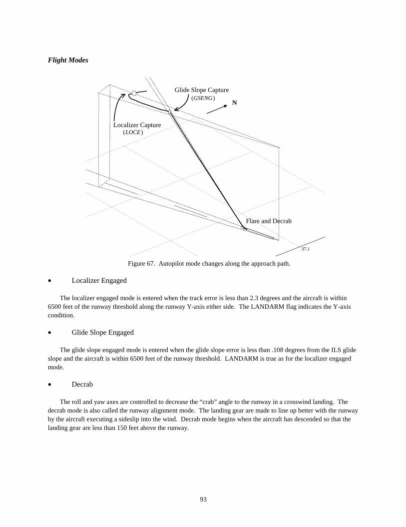
93
Flight Modes
Figure 67. Autopilot mode changes along the approach path.
• Localizer Engaged
The localizer engaged mode is entered when the track error is less than 2.3 degrees and the aircraft is within 6500 feet of the runway threshold along the runway Y-axis either side. The LANDARM flag indicates the Y-axis condition.
• Glide Slope Engaged
The glide slope engaged mode is entered when the glide slope error is less than .108 degrees from the ILS glide slope and the aircraft is within 6500 feet of the runway threshold. LANDARM is true as for the localizer engaged mode.
• Decrab
The roll and yaw axes are controlled to decrease the “crab” angle to the runway in a crosswind landing. The decrab mode is also called the runway alignment mode. The landing gear are made to line up better with the runway by the aircraft executing a sideslip into the wind. Decrab mode begins when the aircraft has descended so that the landing gear are less than 150 feet above the runway.
37.1
N
Localizer Capture
Glide Slope Capture
Flare and Decrab
)(GSENG
)(LOCE

94
• Flare
The FLARE flag is set when the airplane descends below 50 feet above the runway and LANDARM is true. A preprogrammed pitch up rate profile is commanded until the wheels are on the ground. The pitch up rate depends upon the aircraft sink rate. When the wheels are on the ground and spun up, rollout begins and the aircraft pitches down. The simulation stops before rollout for the Airlabs version of B-737 Linear Autoland.
• Rollout
Rollout is a mode that begins when the wheels are on the ground and have spun up. The Airlabs version of the B-737 Linear Autoland stops before this occurs.

95
Engine Model
Figure 68. Turbofan engine.
The engine used in the B-737 linear Autoland model is the Pratt and Whitney JT8D-7. It is an example of the turbofan type of jet engine. A jet engine works by compressing the air and injecting fuel into a combustion chamber. The increase in temperature from the burning of the fuel increases the energy content of the air. This hot air is expanded through a turbine to provide energy to compress new intake air. The energy remaining in the hot air is converted to kinetic energy of motion of the air expelled from the nozzle. A turbofan engine has two compressors in front of the combustion chamber and two turbines following it. Some air from the first compressor is ducted around the combustion chamber and turbines and is called “bypass air”. This is done to increase fuel efficiency by reducing the speed of the nozzle flow but increasing the mass flow.
The primary control parameter of the jet engine is the fuel flow rate into the combustion chamber. The throttle setting controls this fuel flow. The throttle setting is transferred using a cable arrangement to a fuel control unit power lever. The setting of the power lever is called the “cross shaft angle” (CSA).
CSA, Cross shaft angle is the “power lever” fuel flow setting on the fuel control unit for the engine.
FirstCompressor
SecondCompressor
FuelInjector
HighPressureTurbine
Low PressureTurbine
Fan

96
Figure 69. Engine parameter stations.
The equations describing the operation of a turbofan engine use a standard nomenclature of stations from the entrance of the engine to the exit [Ref. 19, p 153]. Station 2 is at the inlet to the engine. Station 3 is at the exit of the first compressor. Station 4 is at the exit of the second turbine. Station 5 is at the entrance to the first turbine. Station 7 is at the exit of the primary nozzle. In [Ref. 13, chapter 1 and 2] is a discussion of the thermodynamic equations that pertain to the turbofan and other jet engines. The station numbering convention is slightly different. Also, many of the equations are expressed in terms of pressure and temperature ratios. The B-737 linear Autoland engine model uses pressure and temperature ratios too, however a different reference is used. [Ref. 13, p 2] uses flight level ambient as the reference p whereas the B-737 linear Autoland uses the International Standard Atmosphere (ISA) value for some of its parameters. The temperature reference is called sea level temperature SLTEMP . Many aircraft parameters for instrumentation use this reference convention to standardize table descriptions [Ref. 2, p 4-3]. The ideal gas law ratio of specific heats for air is used in the equations.
The nomenclature for the thermodynamics of the engine overlaps aeronautics usage for several variables.
Table 9. Engine Symbols that may Cause Confusion with Control Parameter with the Same Name. Symbol
Engine Context
Previous Definition
γ ratio of specific heats of air flight path angle
δ ratio of engine station pressure with a reference
control surface deflection with a subscript denoting which surface
θ ratio of engine station temperature with a reference
Euler pitch angle
72 3 4 5
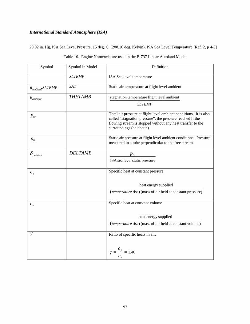
97
International Standard Atmosphere (ISA)
29.92 in. Hg, ISA Sea Level Pressure, 15 deg. C (288.16 deg. Kelvin), ISA Sea Level Temperature [Ref. 2, p 4-3]
Table 10. Engine Nomenclature used in the B-737 Linear Autoland Model
Symbol Symbol in Model Definition
SLTEMP ISA Sea level temperature
SLTEMPtambienθ SAT Static air temperature at flight level ambient
ambientθ THETAMB
SLTEMP
ambient levelflight re temperatustagnation
t0p Total air pressure at flight level ambient conditions. It is also called “stagnation pressure”, the pressure reached if the flowing stream is stopped without any heat transfer to the surroundings (adiabatic).
0p Static air pressure at flight level ambient conditions. Pressure measured in a tube perpendicular to the free stream.
ambientδ DELTAMB
pressure static levelsea ISA
0tp
pc Specific heat at constant pressure
pressure)constant at heldair of (mass rise)
suppliedenergy heat
( etemperatur
vc Specific heat at constant volume
olume)constant vat heldair of (mass rise)
suppliedenergy heat
( etemperatur
γ Ratio of specific heats in air.
40.1==v
p
c
cγ
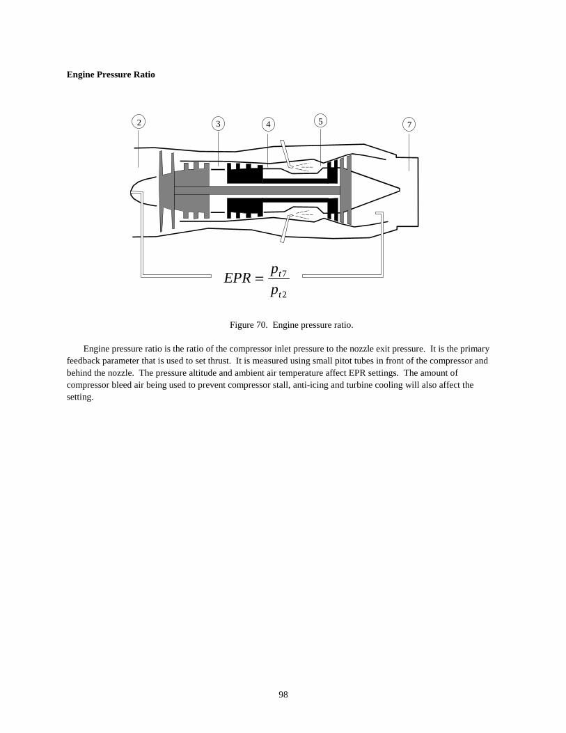
98
Engine Pressure Ratio
Figure 70. Engine pressure ratio.
Engine pressure ratio is the ratio of the compressor inlet pressure to the nozzle exit pressure. It is the primary feedback parameter that is used to set thrust. It is measured using small pitot tubes in front of the compressor and behind the nozzle. The pressure altitude and ambient air temperature affect EPR settings. The amount of compressor bleed air being used to prevent compressor stall, anti-icing and turbine cooling will also affect the setting.
2
7
t
t
p
pEPR =
72 3 4 5
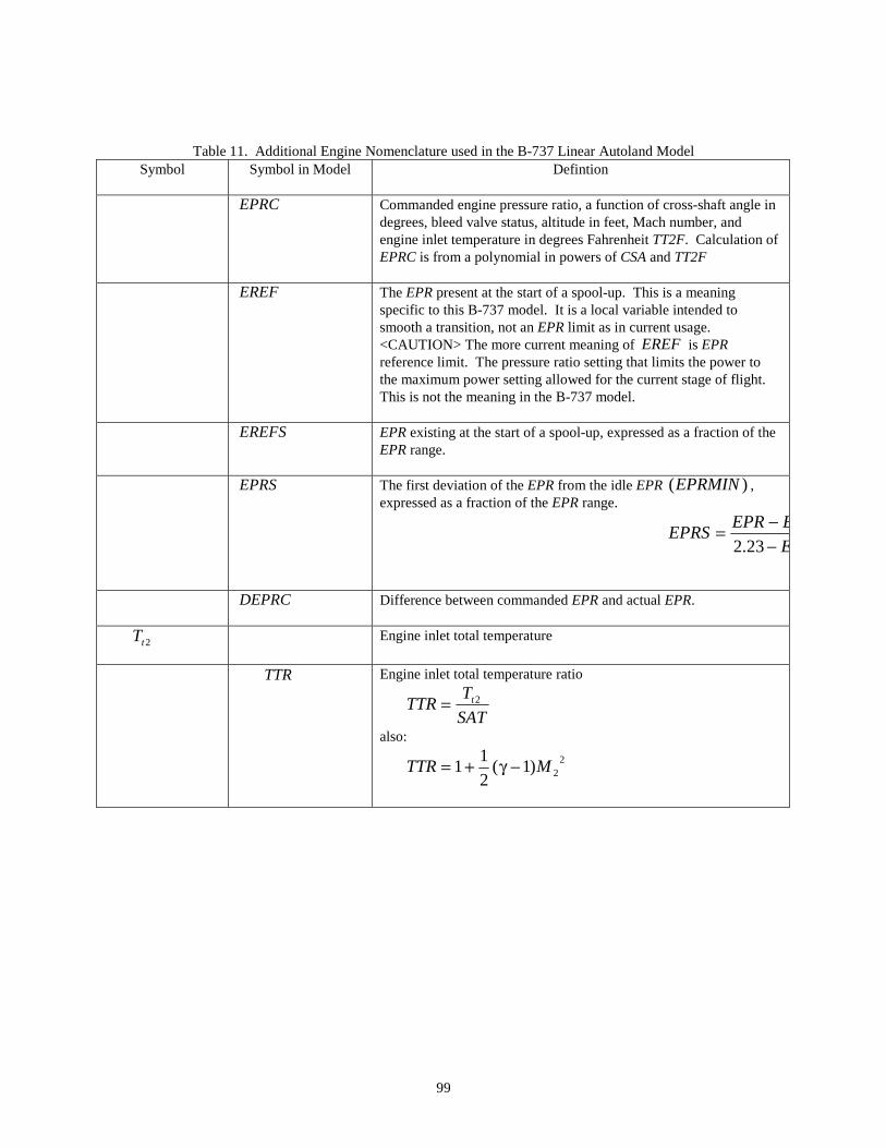
99
Table 11. Additional Engine Nomenclature used in the B-737 Linear Autoland Model Symbol
Symbol in Model
Defintion
EPRC Commanded engine pressure ratio, a function of cross-shaft angle in
degrees, bleed valve status, altitude in feet, Mach number, and engine inlet temperature in degrees Fahrenheit TT2F. Calculation of EPRC is from a polynomial in powers of CSA and TT2F
EREF The EPR present at the start of a spool-up. This is a meaning specific to this B-737 model. It is a local variable intended to smooth a transition, not an EPR limit as in current usage. <CAUTION> The more current meaning of EREF is EPR reference limit. The pressure ratio setting that limits the power to the maximum power setting allowed for the current stage of flight. This is not the meaning in the B-737 model.
EREFS EPR existing at the start of a spool-up, expressed as a fraction of the EPR range.
EPRS The first deviation of the EPR from the idle EPR )(EPRMIN , expressed as a fraction of the EPR range.
EP
EEPREPRS
−−=
23.2
DEPRC Difference between commanded EPR and actual EPR.
2tT Engine inlet total temperature
TTR Engine inlet total temperature ratio
SAT
TTTR t2=
also:
22)1(
2
11 MTTR −γ+=

100
The simplified engine model shown receives a throttle input through the CSA table lookup. The total temperature, aircraft altitude, and Mach number feed the commanded engine pressure (EPRC) ratio calculation. The engine dynamics modifies this based on previous engine EPR profile and bleed valve status and the corrected EPR is sent to the thrust correction for the airframe and flight ambient conditions to get net thrust for the airframe model. The thrust correction module is THCORF and corrects the thrust using a polynomial in powers of Mach number. The spool up detection sets the upper limit on the rate of change of the EPR in the engine dynamics module.
Figure 71. Engine model.
THROTLC
ThrustCorrection
EngineDynamics
EPRCCalculation
THRUST
CSAlookup
CSA
MACH
ALT
T2
BleedValve Logic
Spool-upDetection
PEPRC

101
Compressor Bleed Valve Operation
When the compressor blades turn too fast relative to the air moving through the engine, the effective angle of attack of each compressor blade becomes too great and can stall. Automatic bleed valves in the high-pressure section of the engine (station 3) open to dump air into the fan bypass air duct to increase the velocity of the air moving across the compressor to prevent this stalled condition. This condition can occur if the engine accelerates or decelerates too rapidly and the pressure drop across the compressor is too large. The difference in the static pressure sensed at station three and total pressure sensed at station two controls the operation of the compressor stall bleed valve. The critical EPR for this engine is between 1.110 and 1.128. A family of curves describes the relationship between the fuel control mechanism cross shaft angle (CSA) and the commanded EPR. The curves of commanded EPR as a function of CSA for various Mach numbers from 0 to .95 indicate the critical EPR transition by crossing at this EPR range [Ref. 9]. The bleed valve open logic chooses which curves to use to limit the rate of change of the EPR to account for the action of this valve system.
Compressor bleed air, compressed air from the rear of the compressor stage of the engine is used for deicing, turbine hot structures cooling, and aircraft heating. Engine bleed air can account for a power loss of 30 percent when all anti-icing systems are in use. This model does not account for the engine-deicing configuration.
Figure 72. Engine compressor bleed air.
Bleed ValveLocations
72 3 4 5

102
Figure 73. Engine Simulink diagram.
12
PE
PR
C_
11
TH
CO
RF
10
LE
S_
9
ER
EF
S1
_
8
EP
RS
1_
7
ER
EF
6
EP
RD
OT
5
BV
FLA
G1
_
4
BV
OP
EN
1_
3
EP
RC
2
TH
RU
ST
1
EP
R
xlim
EP
RM
IN
DE
LT
AM
B
MA
CH
EP
R
TH
RU
ST
TH
CO
RF
thru
st_
fun
ctio
n
EP
R
EP
RC
BV
FLA
G
PE
PR
C
ER
EF
S1
ER
EF
_
LE
S_
EP
RS
1
T
PE
PR
C_
ER
EF
LE
S
spo
ol_
up_
dete
ct
==
EP
RC
EP
R_
EP
RD
OT
_
ER
ILA
A
EP
RIL
D
h T
EP
R
EP
RD
OT
__
eng
ine
_dyn
am
ics
0E
PR
CS
A
BV
OP
EN
__
BV
FLA
G_
__
T
BV
OP
EN
_O
R_
CS
A
PR
L11
1_A
ND
_N_
BV
OP
EN
BV
FLA
G
BV
OP
EN
1_
BV
FLA
G1
_
ble
ed_
valv
e_lo
gic
1. +
0.2
* p
ow
(u[1
],2
)
TT
R
TT
2e
ngin
e in
let
1. -
6.8
75
E-6
* u
[1]
TH
ET
AM
B
288
.16
SA
T
EP
R
EP
RM
IN
EP
RA
NG
E
ER
EF
EP
RS
ER
ILA
A
ER
EF
S
ER
ILA
A
AL
T
MA
CH
DE
PR
IDL
E
EP
RID
LE
EP
R_
idle
EP
RA
NG
E
EP
RS
1
EP
RIL
D
EP
RIL
D
CS
A
EP
RID
LE
EP
RC
_
TT
2
BV
OP
EN
_O
R_
CS
A
PR
L11
1_A
ND
_N_
BV
OP
ENE
PR
C
EP
RC
_fun
ctio
n
2.2
3 -
u[1
]
EP
RA
NG
E
EP
R1
_
pow
(u[1
],5
.25
61)
DE
LT
AM
B
TH
RO
TL
CC
SA
CS
A_
fun
ctio
n
15 h
14
PE
PR
C
13
LE
S
12
ER
EF
S1
11
EP
RS
1
10
ER
EF
_
9
EP
RD
OT
_
8
BV
FLA
G_
7
BV
OP
EN
_
6
EP
RC
_
5 T
4
EP
R_
3
TH
RO
TL
C
2
MA
CH
1
AL
T
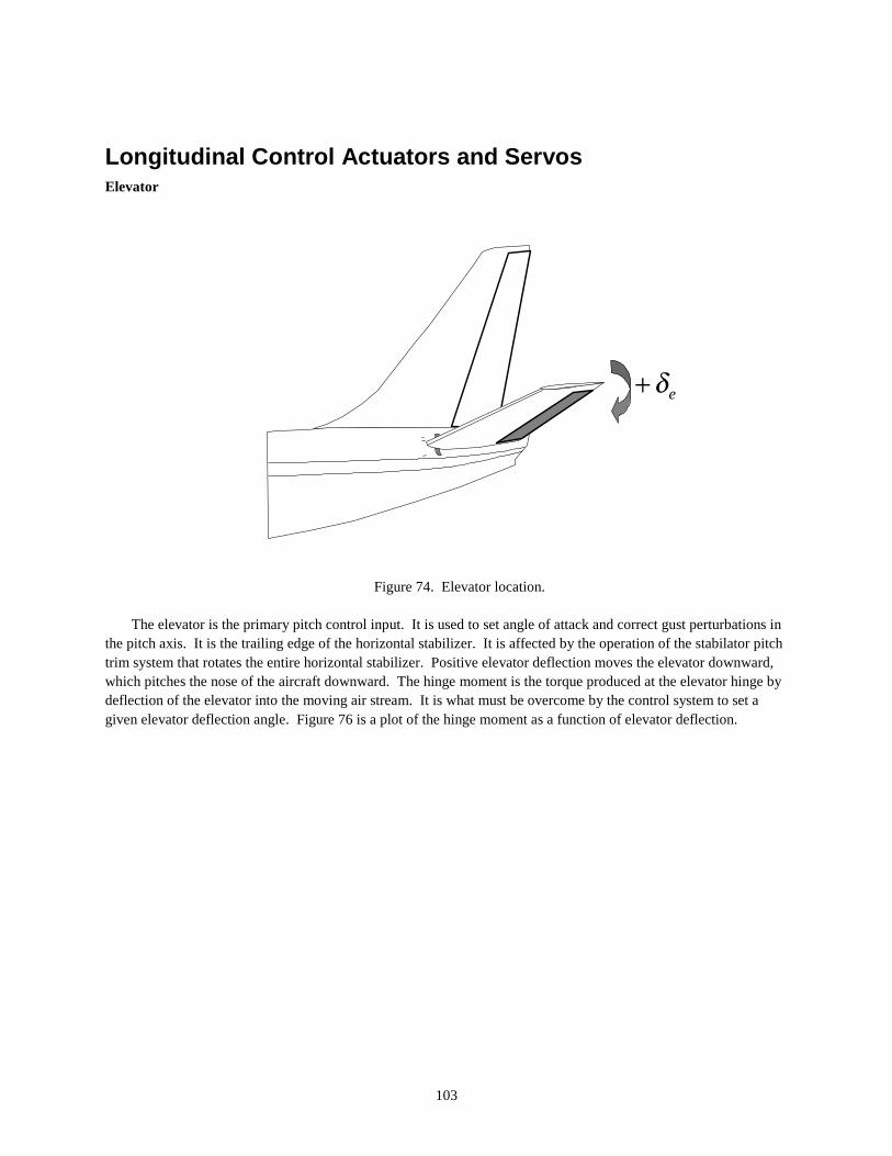
103
Longitudinal Control Actuators and Servos Elevator
Figure 74. Elevator location.
The elevator is the primary pitch control input. It is used to set angle of attack and correct gust perturbations in the pitch axis. It is the trailing edge of the horizontal stabilizer. It is affected by the operation of the stabilator pitch trim system that rotates the entire horizontal stabilizer. Positive elevator deflection moves the elevator downward, which pitches the nose of the aircraft downward. The hinge moment is the torque produced at the elevator hinge by deflection of the elevator into the moving air stream. It is what must be overcome by the control system to set a given elevator deflection angle. Figure 76 is a plot of the hinge moment as a function of elevator deflection.
eδ+
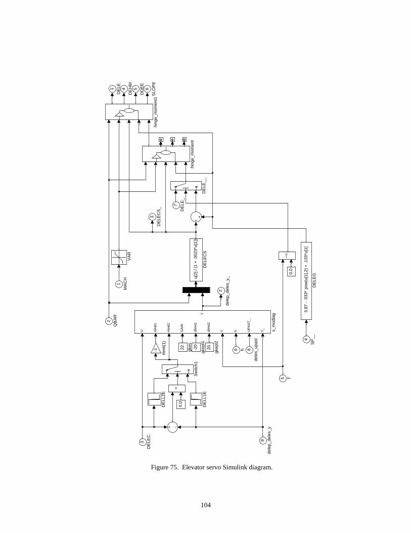
104
Figure 75. Elevator servo Simulink diagram.
6
SLO
PE
5
DD
EE
4
DE
HM
3
DE
LEC
S_
2
dele
p_de
les_
y_
1
DE
LE
U rlim
it1
rlim
it2
GA
IN
dlim
it1
dlim
it2
T h UP
AS
T_
Y_
Y
s_m
odla
g
-1
rlim
it(1)
hing
e_m
omen
t1
hing
e_m
omen
t
22 gkes
20
gkep
l2
-20
gkep
l1
0.0
0.0
VA
R
Sw
itch1
~=
>
DE
LL2E
DE
LL1E
DE
LE__
3.87
- .0
33*
pow
(u[1
],2)
+ .1
33*u
[1]
DE
LEGu[2]
/ (1
+ .0
023*
u[1]
)
DE
LEC
S
9
dele
p_de
les_
y
8
dele
s_up
ast
7
DE
LE_
6 h
5 T
4
SP
__
3
DE
LEC
2
QB
AR
1
MA
CH
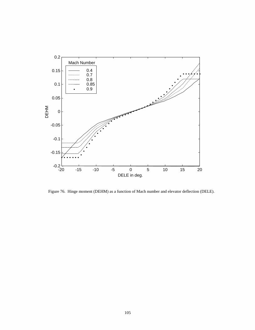
105
Figure 76. Hinge moment (DEHM) as a function of Mach number and elevator deflection (DELE).
-20 -15 -10 -5 0 5 10 15 20-0.2
-0.15
-0.1
-0.05
0
0.05
0.1
0.15
0.2
DELE in deg.
DE
HM
Mach Number
0.40.70.80.850.9
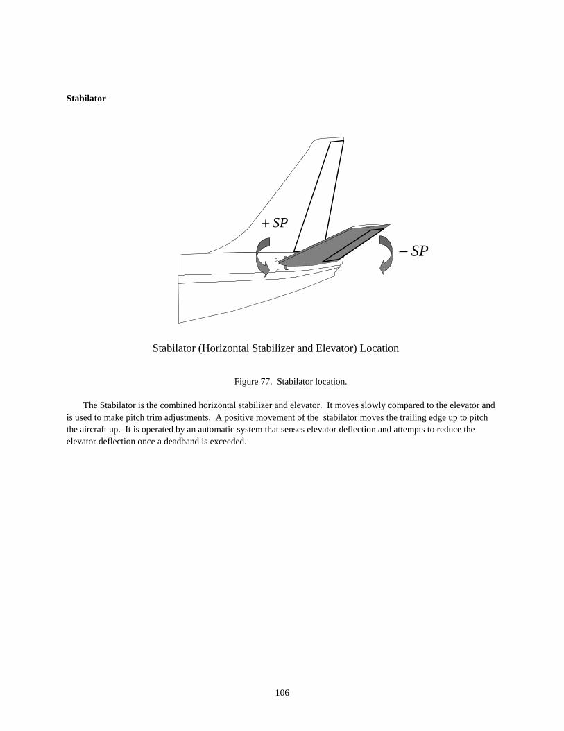
106
Stabilator
Figure 77. Stabilator location.
The Stabilator is the combined horizontal stabilizer and elevator. It moves slowly compared to the elevator and is used to make pitch trim adjustments. A positive movement of the stabilator moves the trailing edge up to pitch the aircraft up. It is operated by an automatic system that senses elevator deflection and attempts to reduce the elevator deflection once a deadband is exceeded.
Stabilator (Horizontal Stabilizer and Elevator) Location
SP+
SP−
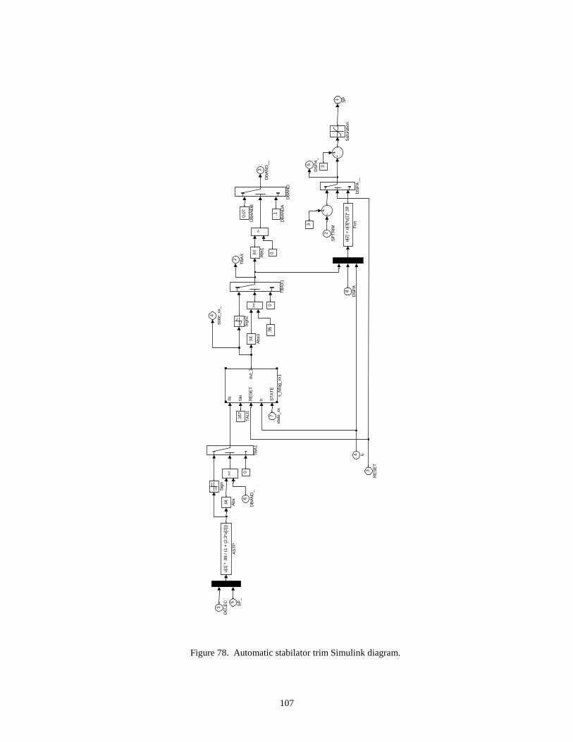
107
Figure 78. Automatic stabilator trim Simulink diagram.
5
DS
PA
_
4
stat
e_xx
_
3
DB
AN
D__
2
TB
AX
1 SP
IN tau
RE
SE
T
h ST
AT
E
out_
1
s_fo
lag_
xx1
0.
3
0
3
.95
0
TB
AX
1
TB
A1
.167
TA
U1
Sig
n2
Sig
n
Sat
urat
ion
>>=
>=
u[2]
+ u
[3]*
u[1]
*.18
Fcn
DS
PA
__
0.07
DB
AN
DB
.1
DB
AN
DA
DB
AN
D
|u|
Abs
3|u
|
Abs
1
|u|
Abs
u[1]
* .8
9 / (
1 +
(2.3
*u[2
]))
AS
TP
8
DS
PA
7
stat
e_xx
6
DB
AN
D_
5
SP
_
4 h3
RE
SE
T
2
SP
TR
IM
1
DE
LEC
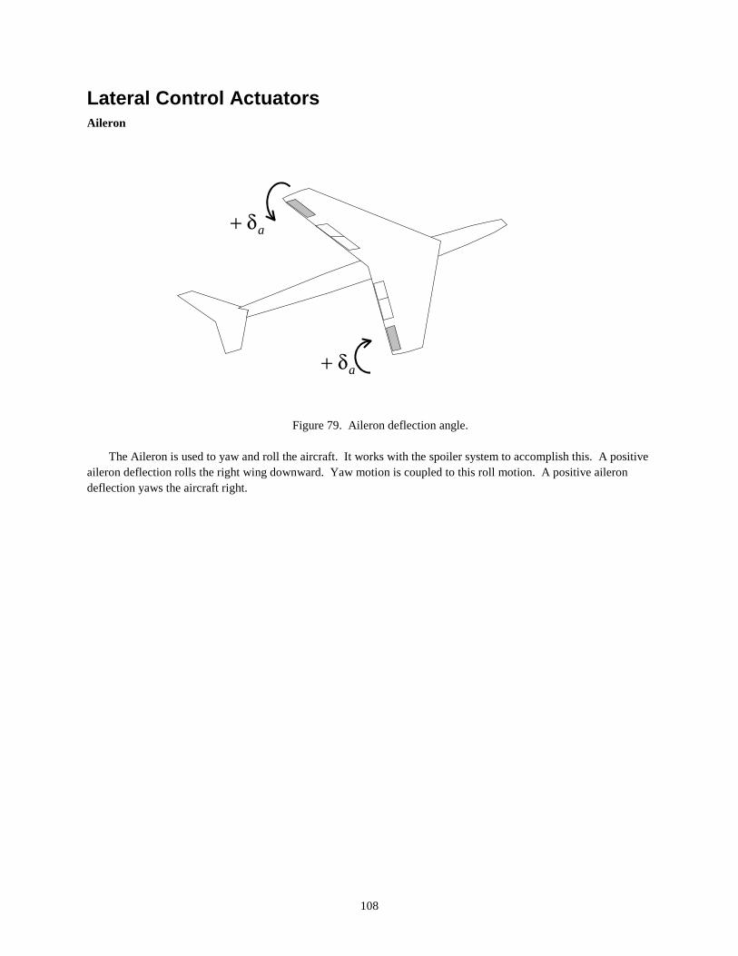
108
Lateral Control Actuators Aileron
Figure 79. Aileron deflection angle.
The Aileron is used to yaw and roll the aircraft. It works with the spoiler system to accomplish this. A positive aileron deflection rolls the right wing downward. Yaw motion is coupled to this roll motion. A positive aileron deflection yaws the aircraft right.
aδ+
aδ+
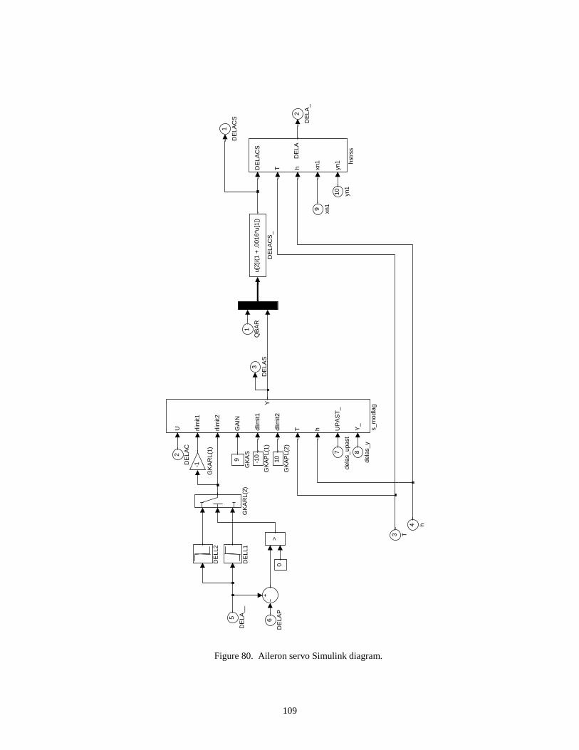
109
Figure 80. Aileron servo Simulink diagram.
3
DE
LAS
2
DE
LA_
1
DE
LAC
S
U rlim
it1
rlim
it2
GA
IN
dlim
it1
dlim
it2
T h UP
AS
T_
Y_
Y
s_m
odla
g
DE
LAC
S
T h xn1
yn1
DE
LA
hstr
ss
0>
9
GK
AS
GK
AR
L(2)
-1
GK
AR
L(1)
10
GK
AP
L(2)
-10
GK
AP
L(1)
DE
LL2
DE
LL1
u[2]
/(1
+ .0
016*
u[1]
)
DE
LAC
S_
10 yn1
9 xn1
8
dela
s_y
7
dela
s_up
ast
6
DE
LAP
5
DE
LA__
4 h
3 T
2
DE
LAC
1
QB
AR
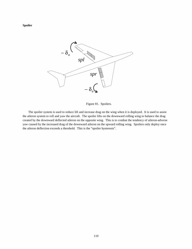
110
Spoiler
Figure 81. Spoilers.
The spoiler system is used to reduce lift and increase drag on the wing when it is deployed. It is used to assist the aileron system to roll and yaw the aircraft. The spoiler lifts on the downward rolling wing to balance the drag created by the downward deflected aileron on the opposite wing. This is to combat the tendency of aileron-adverse yaw caused by the increased drag of the downward aileron on the upward rolling wing. Spoilers only deploy once the aileron deflection exceeds a threshold. This is the “spoiler hysteresis”.
aδ−
aδ−spl
spr

111
Figure 82. Spoiler servo Simulink diagram
Rudder
Figure 83. Rudder and yaw damper location
The rudder is used to control the yaw of the aircraft if the desired yaw is different from that given by the aileron and spoiler system for a given roll. It is mostly commanded automatically through the roll and yaw stability augmentation “yaw damper” system. The lateral control system only commands the rudder during the “decrab” maneuver during the latter phases of an automatic landing.
3
upast_spr_
2
YP_spr_
1
SPR
DELACS
YIC
T
h
YP
out_1
s_sphys
U
rlimit1
rlimit2
GAIN
dlimit1
dlimit2
T
h
UPAST_
Y_
Y
s_modlag
10
gksRS
50
gksRRL2
-50
gksRRL1
40
gksRPL2
0
gksRPL1
Look-Up
Table
4
Gain
7
Y_spr
6
upast_spr
5
YP_spr
4
h
3
T
2
YIC
1
DELACS
rδ+ (Yaw Left)
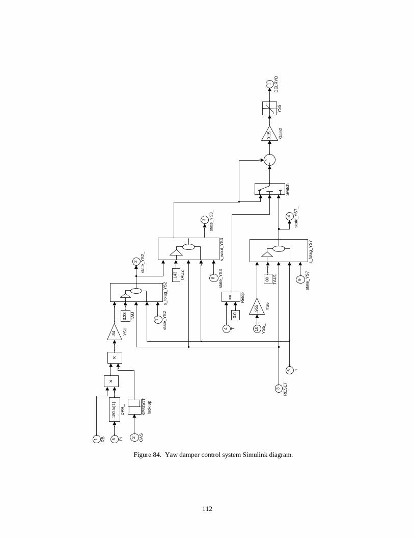
112
Figure 84. Yaw damper control system Simulink diagram.
4
stat
e_Y
S7_
3
stat
e_Y
S3_
2
stat
e_Y
S2_
1
DE
LRY
D
s_w
out_
YS
3
s_fo
lag_
YS
7
s_fo
lag_
YS
2
0.0 .9
55 YS
6
YS
5
.84
YS
1
.143
TA
U2
80
TA
U1
3.33
TA
U
Sw
itch
==
Rel
op
KP
SD
OT
look
up
9.15
Gai
n2
180.
/u[1
]
DP
R_
10
YS
5_
9
stat
e_Y
S7
8
stat
e_Y
S3
7
stat
e_Y
S2
6 h
5 PI
4 T
3
RE
SE
T
2
CA
S
1 RB

113
Approach to Conversion The FORTRAN model was operated using Simulink to call the main functional blocks with FORTRAN Matlab
executable (F-MEX) file blocks. This was done to get confidence with the Simulink method of simulation with the least change to the FORTRAN. Next the feedback loop was broken and the airframe state space model run with constant inputs to see if it would fly at all.
• Deterministic case, no winds and gusts
• Straight and Level Reference Condition
• State Space Equations and Integration and Rates Only
• FORTRAN S-function with Simulink Wrapper
Figure 85. Simulink “wrapper” around FORTRAN deriv and eqmotn with fixed command inputs.
The open loop test was then made closer to the previous runs of the FORTRAN model by taking the time history of the control inputs as input to the airframe state space model without the autopilot present. This method of testing was repeated as parts of the airframe model were replaced with Simulink prototype modules.
in_1
in_2
in_3
in_4
in_5
in_6
in_7
out_1
out_2
out_3
out_4
out_5
out_6
out_7
out_8
out_9
out_10
out_11
out_12
out_13
out_14
out_15
out_16
out_17
out_18
out_19
out_20
out_21
out_22
out_23
out_24
out_25
out_26
out_27
eqmotn
-.0627
const
RB
Yaw Vel
PSI
Yaw
YCG
YCG
XCG
XCG
WB
WB
VGS
VGS
VB
VB
VN
V-northVE
V-eastVD
V-down
UB
UB
8000
Thrust
TKA
TKA
THETAPitch
TAS
TAS
SumSine Wave
0
SPR
0
SPL
3
SPStabilator
PB
Roll VelPHI
Roll
QBAR
QBAR
QB
Pitch Vel
PSIYaw
PHIRoll
MACH
MACH
THETA
LON_2
LON
LON_1
LAT
LAT_1
HCG
HCG
GSE
GSE
GAMMA
GAMMA
ETA
ETA
-.03
DELR
DELE
DELE__
DELE_-5.5
DELE
DELA
DELA
CAS
CAS
ALT
ALT1ALT
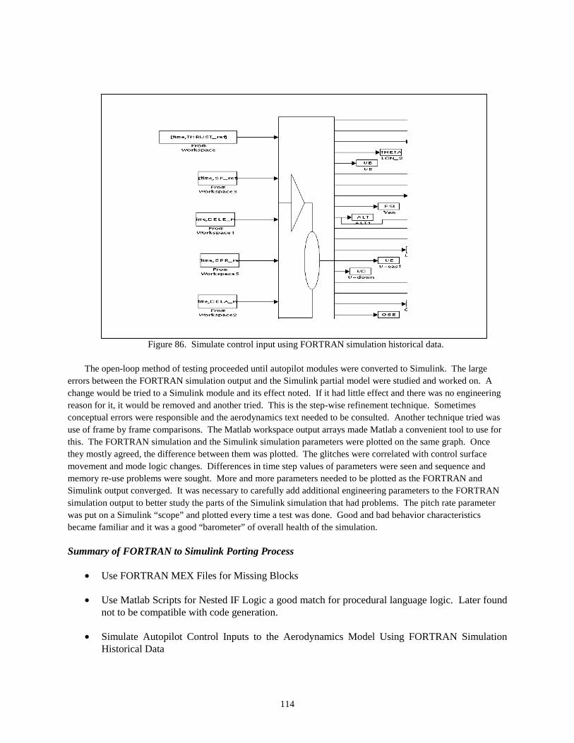
114
Figure 86. Simulate control input using FORTRAN simulation historical data.
The open-loop method of testing proceeded until autopilot modules were converted to Simulink. The large errors between the FORTRAN simulation output and the Simulink partial model were studied and worked on. A change would be tried to a Simulink module and its effect noted. If it had little effect and there was no engineering reason for it, it would be removed and another tried. This is the step-wise refinement technique. Sometimes conceptual errors were responsible and the aerodynamics text needed to be consulted. Another technique tried was use of frame by frame comparisons. The Matlab workspace output arrays made Matlab a convenient tool to use for this. The FORTRAN simulation and the Simulink simulation parameters were plotted on the same graph. Once they mostly agreed, the difference between them was plotted. The glitches were correlated with control surface movement and mode logic changes. Differences in time step values of parameters were seen and sequence and memory re-use problems were sought. More and more parameters needed to be plotted as the FORTRAN and Simulink output converged. It was necessary to carefully add additional engineering parameters to the FORTRAN simulation output to better study the parts of the Simulink simulation that had problems. The pitch rate parameter was put on a Simulink “scope” and plotted every time a test was done. Good and bad behavior characteristics became familiar and it was a good “barometer” of overall health of the simulation.
Summary of FORTRAN to Simulink Porting Process
• Use FORTRAN MEX Files for Missing Blocks
• Use Matlab Scripts for Nested IF Logic a good match for procedural language logic. Later found not to be compatible with code generation.
• Simulate Autopilot Control Inputs to the Aerodynamics Model Using FORTRAN Simulation Historical Data

115
• Open/Closed-Loop Testing
• Use Matlab Workspace to Plot, Plot, Plot...
• It was necessary to modify the FORTRAN simulation to plot additional parameters to better isolate errors.
• Macro error analysis
• Micro error analysis (step-by-step)
• The results of the previous FORTRAN simulation were repeated. It was learned that Matlab needed to be restarted if the test failed to have a valid subsequent test
• Attack easiest and largest errors first.
• Step-wise refinement
• Use Simulink “scope” to monitor QB. It was a good parameter for the pitch loop. Repeat it enough to get used to the pattern so any change is apparent.
• Open loop errors, investigate strongest divergence
Problems Encountered
• Transform to inertial space and divergence of body velocities UB1 and UB2
• Importance of time step alignment for open loop match
• Procedural vs. data flow languages and Integrators. The path not taken still is computed in the Simulink implementation unless explicit steps are taken to block it.
• Different values of pi used in FORTRAN model important for open loop match
• Constant parameters set in the Matlab workspace are not available to S-functions or code generation.

116
Conclusion The Airlabs FORTRAN B-737 Linear Autoland model was duplicated using Matlab/Simulink on several
platforms (Unix, Windows 98 PC). Agreement of the model parameters was achieved to high precision (eight to nine significant figures). Since it is an extension of the B-737 model that was produced with company proprietary data removed, it can be used for research purposes. The Simulink block diagram language is a modern simulation tool and facilitates use by the control system research community.
117
References [1] Barr, N.; Gangsaas, D.; and Schaeffer, D.: Wind Models for Flight Simulator Certification of
Landing and Approach Guidance and Control Systems., FAA-RD-74-206, December 1974.
[2] Cessna Manual of Flight, Jeppesen Sanderson, Inc., 55 Inverness Drive East, Englewood, CO., 1996
[3] Chalk, C.; Neal, T.; Harris, F.; and Pritchard, F.: Background Information and User Guide for MIL-F-8785B(ASG), Military Specification – Flying Qualities of Piloted Airplanes., Technical Report AFFDL-TR-69-72, August, 1967.
[4] DiStefano, J., III; Stubberud, A.; Williams, I.: Schaum’s Outline of Theory and Problems of Feedback and Control Systems, McGraw-Hill Book Company, New York, 1967.
[5] Eshbach, O.; and Souders, M.: Handbook of Engineering Fundamentals, Third Edition, John Wiley and Sons, Inc., New York, 1975.
[6] Etkin, B.: Dynamics of Flight, John Wiley & Sons, New York, 1959.
[7] Friedland, B.: Control System Design, An Introduction to State Space Methods, McGraw-Hill, Inc., New York, 1986.
[8] Gainer, T.; and Hoffman, S.: Summary of Transformation Equations and Equations of Motion Used in Free Flight and Wind-Tunnel Data Reduction And Analysis., Appendix A, page 67, NASA SP-3070, 1972.
[9] Guenther, A.: Linear 737 Autoland Simulation for Airlabs, Sperry Corporation, Systems Management Group, Hampton, VA, Publication Number SP710-032, Contract NAS1-17929, 1985.
[10] Gupta, S.; and Hasdorff, L.: Fundamentals of Automatic Control, John Wiley & Sons, Inc., New York, 1970
[11] Halliday, D.; and Resnick, R.: Fundamentals of Physics, John Wiley & Sons, Inc., New York, 1970, p 197.
[12] Klawans, B.: Simple Method for Calculating the Characteristics of the Dutch Roll Motion of an Airplane., NACA-TN-3754, 1956.
[13] Kerrebrock, J.: Aircraft Engines and Gas Turbines, MIT Press, Cambridge, Massachusetts, 1977
[14] Kroes, M., Wild, T., Bent, R., and McKinley, J., Aircraft Powerplants, Sixth Edition, McGraw-Hill Inc., New York, 1990
[15] Ogata, K.: Discrete-Time Control Systems, Prentice-Hall, Inc., New Jersey, 1987
118
[16] Press, H.; and Meadows, M. T.: A Re-evaluation of Gust-Load Statistics for Applications in Spectral Calculations., NACA-TN-3540, 1955.
[17] Press, W.; Teukolsky, S.; Vetterling, W.; Flannery, B.: Numerical Recipes in C The Art of Scientific Computing, Second Edition, Cambridge University Press, Cambridge CB2 1RP, 1992.
[18] Ragazzini, J.R.; and Bergen, A.R.: A Mathematical Technique for the Analysis of Linear Systems. Proceedings of the IRE, Vol 42, No 11, November 1954, pp. 1641-1657.
[19] Treager, I. E.; Aircraft Gas Turbine Engine Technology (Aviation Technology Series), Third Edition, Glenco/McGraw-Hill, New York, 1996
[20] Seckel, E., Stability and Control of Airplanes and Helicopters, Academic Press, New York, 1964
[21] U.S. Standard Atmosphere, 1962, Washington 25, D.C., Bureau of Documents, Government Printing Office
REPORT DOCUMENTATION PAGE Form ApprovedOMB No. 0704-0188
2. REPORT TYPE
Contractor Report 4. TITLE AND SUBTITLE
B-737 Linear Autoland Simulink Model5a. CONTRACT NUMBER
NAS1-00135
6. AUTHOR(S)
Hogge, Edward F.
7. PERFORMING ORGANIZATION NAME(S) AND ADDRESS(ES)
Lockheed MartinHampton, VA 23681-2199
9. SPONSORING/MONITORING AGENCY NAME(S) AND ADDRESS(ES)
National Aeronautics and Space AdministrationWashington, DC 20546-0001
8. PERFORMING ORGANIZATION REPORT NUMBER
10. SPONSOR/MONITOR'S ACRONYM(S)
NASA
13. SUPPLEMENTARY NOTESLangley Technical Monitor: Celeste BelcastroAn electronic version can be found at http://techreports.larc.nasa.gov/ltrs/ or http://ntrs.nasa.gov
12. DISTRIBUTION/AVAILABILITY STATEMENTUnclassified - UnlimitedSubject Category 08Availability: NASA CASI (301) 621-0390 Distribution: Standard
19a. NAME OF RESPONSIBLE PERSON
STI Help Desk (email: [email protected])
14. ABSTRACT
The Linear Autoland Simulink model was created to be a modular test environment for testing of control system components in commercial aircraft. The input variables, physical laws, and referenced frames used are summarized. The state space theory underlying the model is surveyed and the location of the control actuators described. The equations used to realize the Dryden gust model to simulate winds and gusts are derived. A description of the pseudo-random number generation method used in the wind gust model is included. The longitudinal autopilot, lateral autopilot, automatic throttle autopilot, engine model and automatic trim devices are considered as subsystems. The experience in converting the Airlabs FORTRAN aircraft control system simulation to a graphical simulation tool (Matlab/Simulink) is described.
15. SUBJECT TERMS14. SUBJECT TERMS
Aircraft simulation; Wind gust model; Control system; Autopilot; Computer model; State space model; Aircraft dynamics; Equations of motion; Commercial aircraft
18. NUMBER OF PAGES
123
19b. TELEPHONE NUMBER (Include area code)
(301) 621-0390
a. REPORT
U
c. THIS PAGE
U
b. ABSTRACT
U
17. LIMITATION OF ABSTRACT
UU
Prescribed by ANSI Std. Z39.18Standard Form 298 (Rev. 8-98)
3. DATES COVERED (From - To)
5b. GRANT NUMBER
5c. PROGRAM ELEMENT NUMBER
5d. PROJECT NUMBER
5e. TASK NUMBER
5f. WORK UNIT NUMBER
23-728-30-10
11. SPONSOR/MONITOR'S REPORT NUMBER(S)
NASA/CR-2004-213021
16. SECURITY CLASSIFICATION OF:
The public reporting burden for this collection of information is estimated to average 1 hour per response, including the time for reviewing instructions, searching existing data sources, gathering and maintaining the data needed, and completing and reviewing the collection of information. Send comments regarding this burden estimate or any other aspect of this collection of information, including suggestions for reducing this burden, to Department of Defense, Washington Headquarters Services, Directorate for Information Operations and Reports (0704-0188), 1215 Jefferson Davis Highway, Suite 1204, Arlington, VA 22202-4302. Respondents should be aware that notwithstanding any other provision of law, no person shall be subject to any penalty for failing to comply with a collection of information if it does not display a currently valid OMB control number.PLEASE DO NOT RETURN YOUR FORM TO THE ABOVE ADDRESS.
1. REPORT DATE (DD-MM-YYYY)
05 - 200401-