Azhar University Civil Engineering Second Year Civil

Computer Applications

 

 

INTRODUCTION 

   

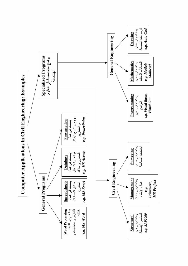
Civil Engineering Computer Application Second Year Civil Introduction: Similar to many other professions, Civil Engineering has become highly depended on computers for delivering different work tasks. Starting from conceptual design up to finalization of the construction, the role of computer software is becoming more and more important. The goal of this course is to give general information about programs that are currently used in the field of civil engineering. Examples of some civil engineering problems and the software applications used to solve them are presented. Due to the huge number of software programs available the given examples are by no way comprehensive. However, these examples serve as an introduction to inform students about the different ways a computer software can facilitate and enhance their work. The course also aims at encouraging students to explore more ways of enhancing their work by using computer software. Software Categories: Software used in civil engineering applications can be classified into (See Fig. 1):

General software such as o word processing, e.g. MS Word o Spreadsheets, e.g. MS Excel o Database software, e.g. MS Access o Presentation Software, such as MS Power Point

Specialized software which are oriented towards engineering applications and these can be classified into general engineering software or civil engineering software. Civil Engineering software can be further classified into specialized Engineering software such as Structural Engineering, Surveying or Construction Management

o General Engineering Software like AutoCAD and Mathcad o BIM and 3D modeling software such as Autodesk REVIT o Structural Engineering Software such as SAP2000, ETABS, SAFE and

STAAD o Structural Detailing software like Autodesk Structural Detailing o Structural Steel Shop drawings software like TEKLA o Surveying software such as Surfer o Road design software such as Autodesk Civil 3D o Irrigation and water flow software such as GMS SEEP2D o Soil Analysis software such as Plaxis o Construction Management software such as Primavera and MS Project

Com

pute

r A

pplic

atio

ns in

Civ

il E

ngin

eeri

ng: E

xam

ples

Gen

eral

Pro

gram

sSp

ecia

lized

Pro

gram

sوملعلى اة فصصتخ ممجبرا

يةدسهنال

Wor

d Pr

oces

sing

بة آتا

ى م فخدستي

و ت اباخط ال ويرارلتقا

لافه خ

e.g.

MS

Wor

d

Spre

adsh

eets

مل عفى

دم تخيس

ت اباحس للولجدا

رة كرلمت ا

e.g.

MS

Exc

el

Dat

abas

eمل عفى

دم تخيس

ثل ت م

انا بيعدقوا

لافه خ وزنخاالم

e.g.

MS

Acc

ess

Pres

enta

tion

مل عفى

دم تخيس

ارفكالأ

ح شرض ل

روع

يع ارمش الأو

e.g.

Pow

erP

oin

t

Civ

il E

ngin

eeri

ngG

ener

al E

ngin

eeri

ng

Dra

win

gمل عفى

دم تخيس

سية هند التومارسال

e.g.

Au

to C

ad

Mat

hem

atic

sمل عفى

دم تخيس

قدة مع التاباحسال

e.g.

Mat

lab,

M

ath

cad

Prog

ram

min

gمل عفى

دم تخيس

مجراالب

e.g.

Vis

ual

Bas

ic,

Vis

ual

C+

+

Surv

eyin

gب سا حفى

دم تخيس

حية ساالم

ت لياعمال

Man

agem

ent

رةإدا

ى م فخدستي

شاء لإنل اعما

أe.

g.

Pri

mav

era,

M

S P

roje

ct

Stru

ctur

alل حفى

دم تخيس

ئية شالإنر اصعناال

e.g.

SA

P20

00

 

 

Math CAD 

 

 

 

 

Using Mathcad in Civil Engineering Applications 

Mathcad is a mathematical program that can perform numerical and symbolic calculations 

and mathematical operations that can solve many engineering problems. 

In the following pages examples of using Mathcad in civil engineering problems will be 

presented 

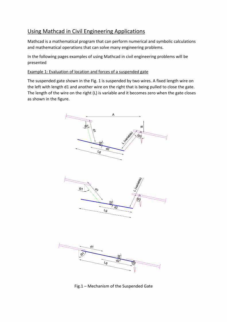
Example 1: Evaluation of location and forces of a suspended gate 

The suspended gate shown in the Fig. 1 is suspended by two wires. A fixed length wire on 

the left with length d1 and another wire on the right that is being pulled to close the gate. 

The length of the wire on the right (L) is variable and it becomes zero when the gate closes 

as shown in the figure. 

 

Fig.1 – Mechanism of the Suspended Gate 

As shown in the Fig. 2, the geometric location of the gate is defined by the following 

parameters: 

The variable parameters Θ1, Θ2, Θ3, L and the fixed parameters Lg, d1, d2, A, and B. 

 

Fig.2. Geometric Configuration of the suspended Gate 

The geometric configuration of the gate produces the following two equations: 

d1 Sin Θ1 + d2 Cos Θ2 + L Sin Θ3= A (1)

d1 Cos Θ1 + d2 Sin Θ2 - L Cos Θ3= B (2)

 

The Gate is subjected to three forces, Wg, the weight of the gate, T1 and T2 the tension in 

the left and right cables, respectively as shown in Fig. 3.  The equilibrium of the forces 

produces the following 3 equations: 

ΣFx= 0 -T1 Sin Θ1 + T2 Sin Θ2 =0 (3)

ΣFy= 0 T1 Cos Θ1 + T2 Cos Θ2 ‐ Wg =0 (4)

ΣMo= 0 T1 Cos Θ1 x d2 Cos Θ2 - T1 Sin Θ1 x d2 Sin Θ2 – Wg x dw x Cos Θ2 =0 (5)

Where dw is the distance from the c.g. to point O.  

 

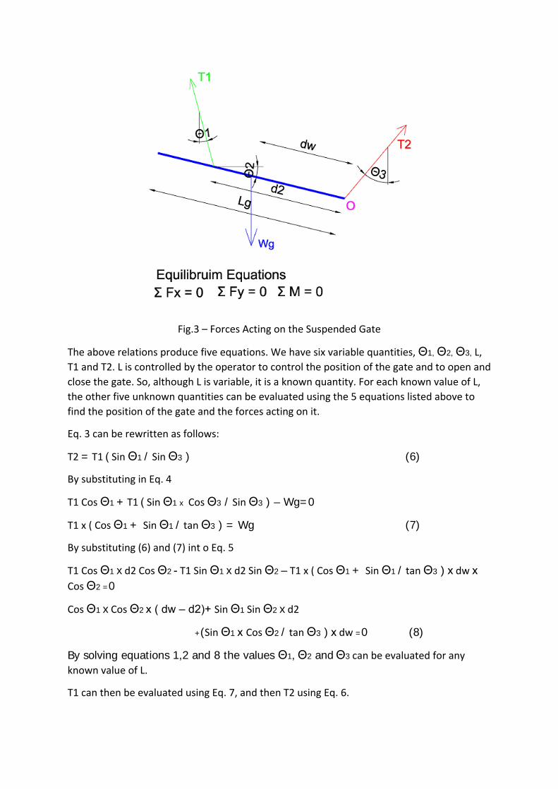
Fig.3 – Forces Acting on the Suspended Gate 

The above relations produce five equations. We have six variable quantities, Θ1, Θ2, Θ3, L, 

T1 and T2. L is controlled by the operator to control the position of the gate and to open and 

close the gate. So, although L is variable, it is a known quantity. For each known value of L, 

the other five unknown quantities can be evaluated using the 5 equations listed above to 

find the position of the gate and the forces acting on it.  

Eq. 3 can be rewritten as follows: 

T2 = T1 ( Sin Θ1 / Sin Θ3 ) (6)

By substituting in Eq. 4  

T1 Cos Θ1 + T1 ( Sin Θ1 x Cos Θ3 / Sin Θ3 ) – Wg=0

T1 x ( Cos Θ1 + Sin Θ1 / tan Θ3 ) = Wg (7)

By substituting (6) and (7) int o Eq. 5 

T1 Cos Θ1 x d2 Cos Θ2 - T1 Sin Θ1 x d2 Sin Θ2 – T1 x ( Cos Θ1 + Sin Θ1 / tan Θ3 ) x dw x Cos Θ2 =0

Cos Θ1 x Cos Θ2 x ( dw – d2)+ Sin Θ1 Sin Θ2 x d2 

+(Sin Θ1 x Cos Θ2 / tan Θ3 ) x dw =0 (8)

By solving equations 1,2 and 8 the values Θ1, Θ2 and Θ3 can be evaluated for any 

known value of L. 

T1 can then be evaluated using Eq. 7, and then T2 using Eq. 6. 

This can be done in Mathcad according to the following steps: 

1. The known values for A, B, L, dw, d1, d2 and Wg are input in Mathcad as shown 

below 

 2. The solution of the values of Θ1, Θ2 and Θ3 are obtained using the command 

Given Find in math cad where Θ1, Θ2 and Θ3 are trial values then a Given 

statement is issued followed by the three equations to be solved then this is 

followed by the command Find ( Θ1, Θ2, Θ3 ) to find the values of Θ1, Θ2 and Θ3

that satisfies the three equations. The Mathcad commands are as follows: 

 3. After the values of Θ1, Θ2 and Θ3 have been evaluated, the values of T1 and T2 can 

be evaluated using the following commands: 

 The Complete solution using Mathcad is presented in Fig.4 

 

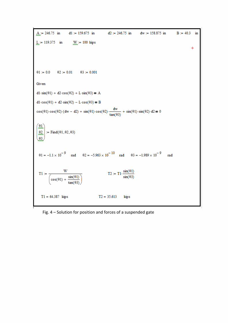
 Fig. 4 – Solution for position and forces of a suspended gate 

 

 

 

   

Example 2:  Designing of double steel angles subjected to compression force using Mathcad 

 

Consider a double steel angle subjected to compression Force N. The actual stress on the 

angles will be evaluated as Fact = N/2A where A is the area of the single angle. 

This stress should be less than the allowable stress Fc: 

Fact <= Fc 

The allowable stress Fc of a compression member is dependent on the maximum 

slenderness ratio λmax, which is equal to the length L divided by the radius of gyration of the section (r).  The double angle has two radii of gyrations rx and ry, where Ix= 2A rx2 and Iy= 2A ry2, where Ix and Iy are the moment of inertia of the double angles about the X and Y axes, respectively. Assuming that the unconfined length in the x and y directions is equal to the length of the 

compression member, L, then we will obtain 2 slenderness ratios: 

λx= L / rx and λy= L / ry For the double angle rx is equal to rx of the single angle and is always smaller than ry, so λx will always be smaller than λy (λx< λy). Or λmax= λx =. L / rx.  

After obtaining λmax we can find the allowable stress Fc as follows:

If  λmax <= 100  then the allowable stress Fc is evaluated as : 

 

But if  λmax > 100 , Fc will be evaluated as: 

 

The Last step is to compare the actual stress Fact to the allowable stress Fc to make sure 

that Fact < =Fc. 

This problem is solved in Mathcad as follows: 

First the values of the normal force (N), Length (L) and Yield Strength of steel (σy) are 

input in Mathcad as follows: 

  Next a trial angle is chosen for example L100x100x10, and the value of its area and 

radius of gyration (A and rx) are input in Mathcad as follows 

 Note: the input area A is for one angle, so 2A is used in the equations because 

double angle is used. 

The program calculates the slenderness ratio λmax  using its equation as follows: 

  Because the calculation of the actual stress Fc uses one of 2 equations depending on 

the value of λmax, this calculation is performed using the (if otherwise) command in 

Mathcad as shown below: 

  Finally, a check is performed to find if the section is safe. If Fact < Fc then the section 

is OK, otherwise, the section is not OK. The check is done using the (if otherwise) 

command as shown below: 

  Other sections can be checked by changing the values of A and rx according to the 

properties of the chosen angle. Mathcad will automatically perform the calculations 

to check the new section.  

The calculations will also be adjusted if the Normal force, the yield strength or the 

member length were changed. 

The complete Mathcad file for this example is shown in Fig. 5. 

 

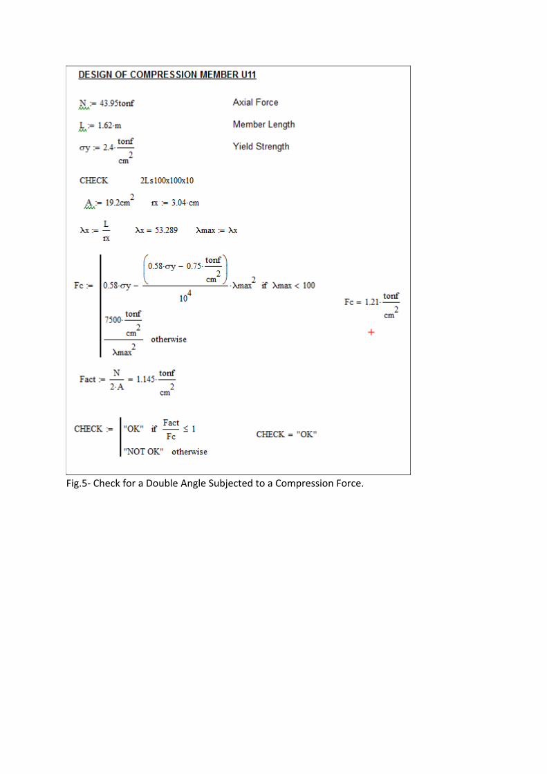
 Fig.5‐ Check for a Double Angle Subjected to a Compression Force. 

  

 

 

 

 

 

AUTOCAD 

   

Civil Engineering Computer Application -AutoCAD Second Year Civil Example 1: Drawing an excavation cross section and finding the area of excavation

Solution :

1) Open the AutoCAD program. A new file is Opened by default. From the Menu Choose File-> Save As and save the file to the name “CA_5.dwg”. 2) Draw the line that represents the excavation. Type the Line command or choose it

from the Menu. Input the following 0,0 Enter 4, -3 Enter16, -3 Enter 20,0 Enter Enter Tip: Make sure dynamic Input is OFF A Line as shown in Fig. 1 will be drawn.

3) Draw the line that represents the natural soil level. Type the PLine command or choose it from the Menu. Input the following 0,1.25 Enter 2, 1.05 Enter4, 0.85 Enter 6,0.95 Enter 8,1.1 Enter 10, 0.8 Enter 12, 0.75 Enter 14,0.8 Enter 16,0.7 Enter 18,0.9 Enter 20,0.8 Enter Enter. A polyline representing the natural soil profile is drawn as shown in Fig. 2

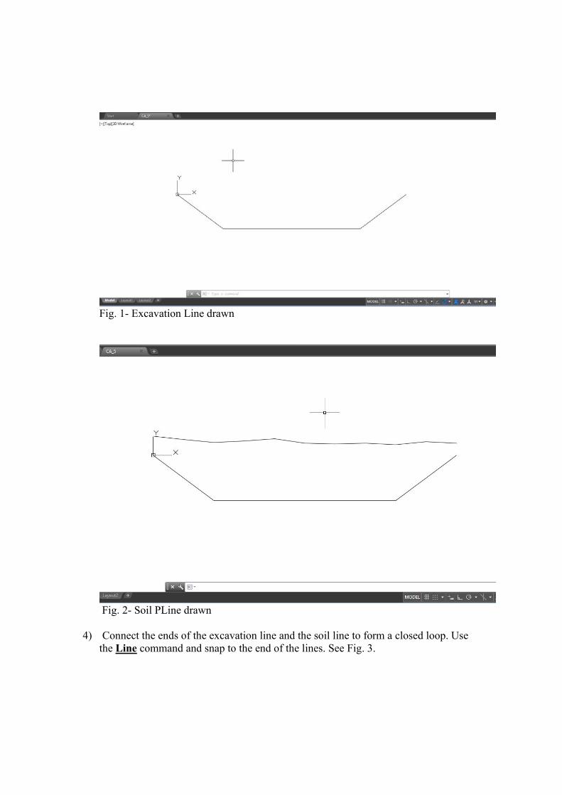
Fig. 1- Excavation Line drawn

Fig. 2- Soil PLine drawn

4) Connect the ends of the excavation line and the soil line to form a closed loop. Use the Line command and snap to the end of the lines. See Fig. 3.

Fig. 3- Making a closed loop (connecting the excavation and soil lines) 5) Transform the closed loop into one polyline entity by using the PEdit:Join

Command. Use the PEdit Command, choose the soil polyline, then click on the Join command, and then choose all the lines in the loop, then press Enter. The loop will be transformed into one polyline entity.

6) To find the area of the excavation use the command List and choose the closed polyline. The information about the polyline including the area and perimeter is listed as shown in Fig. 4. The area is listed as 65.85 m2.

Fig. 4 – List of the closed polyline properties.

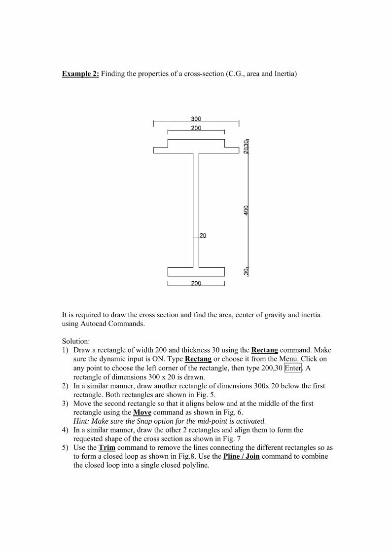
Example 2: Finding the properties of a cross-section (C.G., area and Inertia)

It is required to draw the cross section and find the area, center of gravity and inertia using Autocad Commands. Solution: 1) Draw a rectangle of width 200 and thickness 30 using the Rectang command. Make

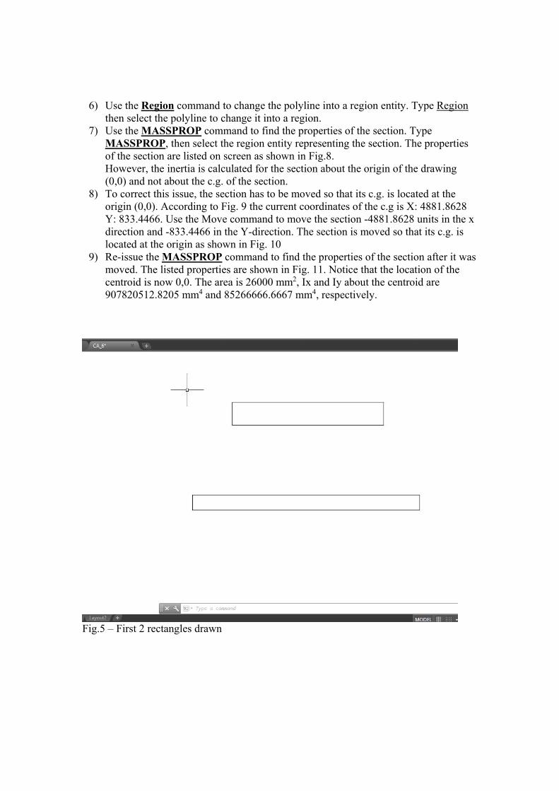
sure the dynamic input is ON. Type Rectang or choose it from the Menu. Click on any point to choose the left corner of the rectangle, then type 200,30 Enter. A rectangle of dimensions 300 x 20 is drawn.

2) In a similar manner, draw another rectangle of dimensions 300x 20 below the first rectangle. Both rectangles are shown in Fig. 5.

3) Move the second rectangle so that it aligns below and at the middle of the first rectangle using the Move command as shown in Fig. 6. Hint: Make sure the Snap option for the mid-point is activated.

4) In a similar manner, draw the other 2 rectangles and align them to form the requested shape of the cross section as shown in Fig. 7

5) Use the Trim command to remove the lines connecting the different rectangles so as to form a closed loop as shown in Fig.8. Use the Pline / Join command to combine the closed loop into a single closed polyline.

6) Use the Region command to change the polyline into a region entity. Type Region then select the polyline to change it into a region.

7) Use the MASSPROP command to find the properties of the section. Type MASSPROP, then select the region entity representing the section. The properties of the section are listed on screen as shown in Fig.8. However, the inertia is calculated for the section about the origin of the drawing (0,0) and not about the c.g. of the section.

8) To correct this issue, the section has to be moved so that its c.g. is located at the origin (0,0). According to Fig. 9 the current coordinates of the c.g is X: 4881.8628 Y: 833.4466. Use the Move command to move the section -4881.8628 units in the x direction and -833.4466 in the Y-direction. The section is moved so that its c.g. is located at the origin as shown in Fig. 10

9) Re-issue the MASSPROP command to find the properties of the section after it was moved. The listed properties are shown in Fig. 11. Notice that the location of the centroid is now 0,0. The area is 26000 mm2, Ix and Iy about the centroid are 907820512.8205 mm4 and 85266666.6667 mm4, respectively.

Fig.5 – First 2 rectangles drawn

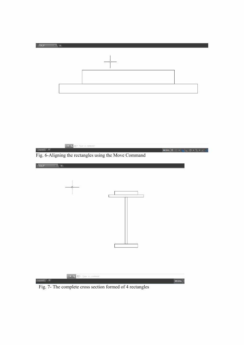
Fig. 6-Aligning the rectangles using the Move Command

Fig. 7- The complete cross section formed of 4 rectangles

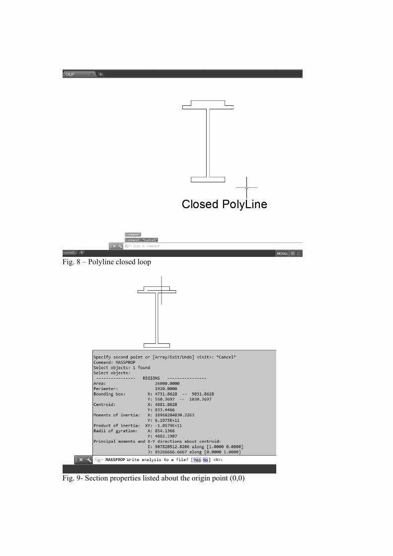
Fig. 8 – Polyline closed loop

Fig. 9- Section properties listed about the origin point (0,0)

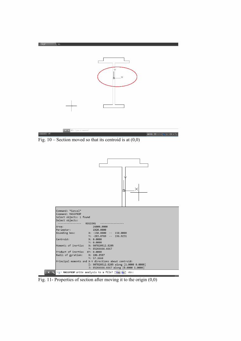
Fig. 10 – Section moved so that its centroid is at (0,0)

Fig. 11- Properties of section after moving it to the origin (0,0)

Example 3: Finding the properties of a non-symmetric cross-section (C.G., area and Inertia and principal axes)

It is required to draw the cross section and find the area, center of gravity, inertia and principal axes using AutoCAD Commands. Solution:

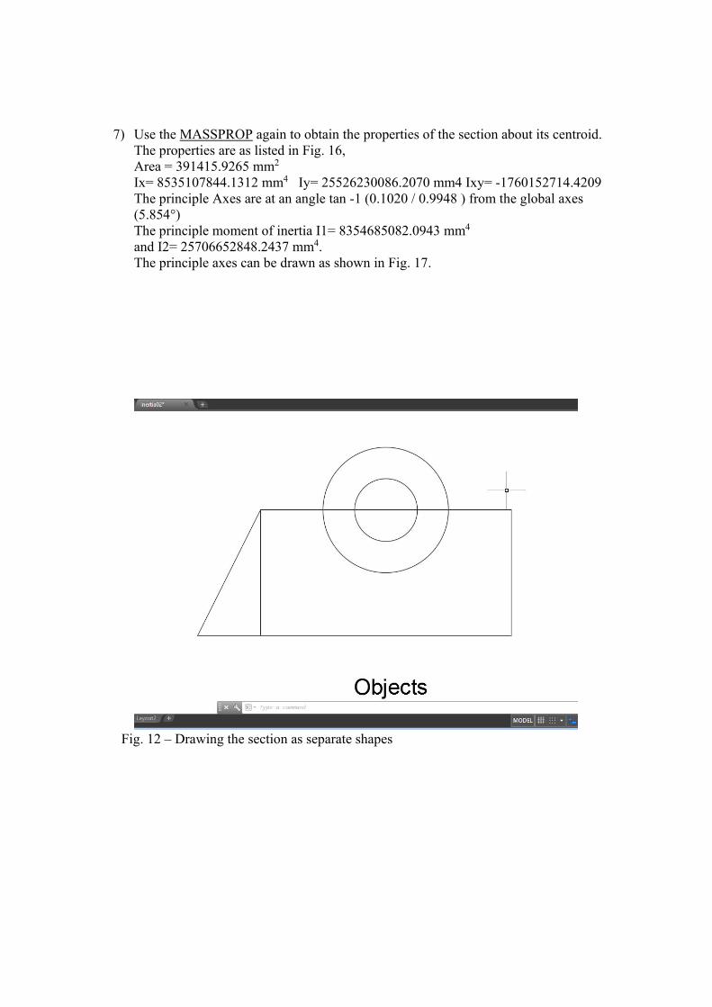
1) Draw a rectangle of width 800 and thickness 400 using the Rectang command. Draw two circles of radii 100 and 200 using the Circle command. Use the Line command to draw the inclined line on left of the shape. Move the shapes in the correct position using the Move command to obtain the shape shown in Fig. 12.

2) Use the Trim command to make an outer closed loop as shown in Fig. 13. 3) Use the PEdit/Join command to transfer the outer loop into a single polyline. 4) Use the Region command and select the outer polyline and the inner circle to change

both into a region (two regions are drawn). 5) Combine the two regions into one region by using the Subtract command. Type the

Subtract command, next select the outer region, the press Enter, then select the inner circle then press Enter. The two regions are combined into one region (An outer region with a hole).

6) Use the MASSPROP command to find the properties of the formed region. The list of properties is as shown in Fig. 14. However, the inertias are calculated about the origin of the coordinates (0,0). In order to obtain the correct values of the inertias the shape has to be moved so that its c.g is moved to point 0,0. According to Fig. 14 the current coordinates of the c.g is X= 28984.0616 and Y= 1743.8513. Use the Move command to move the shape -28984.0616 in the X direction and -1743.8513 in the Y-direction. The shape is moved with its c.g at the origin as shown in Fig. 15.

7) Use the MASSPROP again to obtain the properties of the section about its centroid. The properties are as listed in Fig. 16, Area = 391415.9265 mm2 Ix= 8535107844.1312 mm4 Iy= 25526230086.2070 mm4 Ixy= -1760152714.4209 The principle Axes are at an angle tan -1 (0.1020 / 0.9948 ) from the global axes (5.854°) The principle moment of inertia I1= 8354685082.0943 mm4 and I2= 25706652848.2437 mm4. The principle axes can be drawn as shown in Fig. 17.

Fig. 12 – Drawing the section as separate shapes

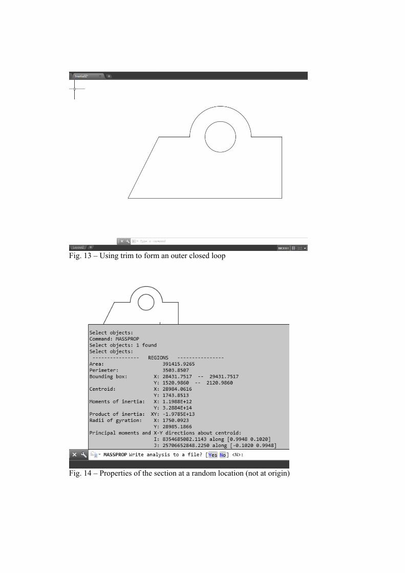
Fig. 13 – Using trim to form an outer closed loop

Fig. 14 – Properties of the section at a random location (not at origin)

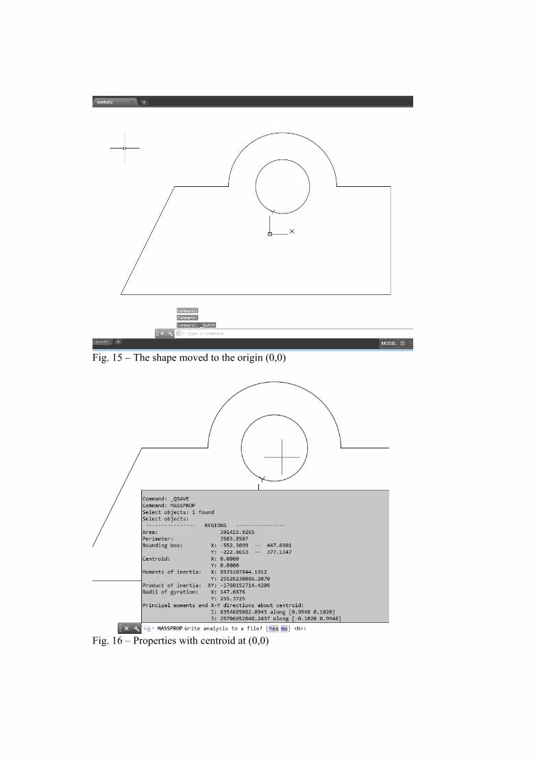
Fig. 15 – The shape moved to the origin (0,0)

Fig. 16 – Properties with centroid at (0,0)

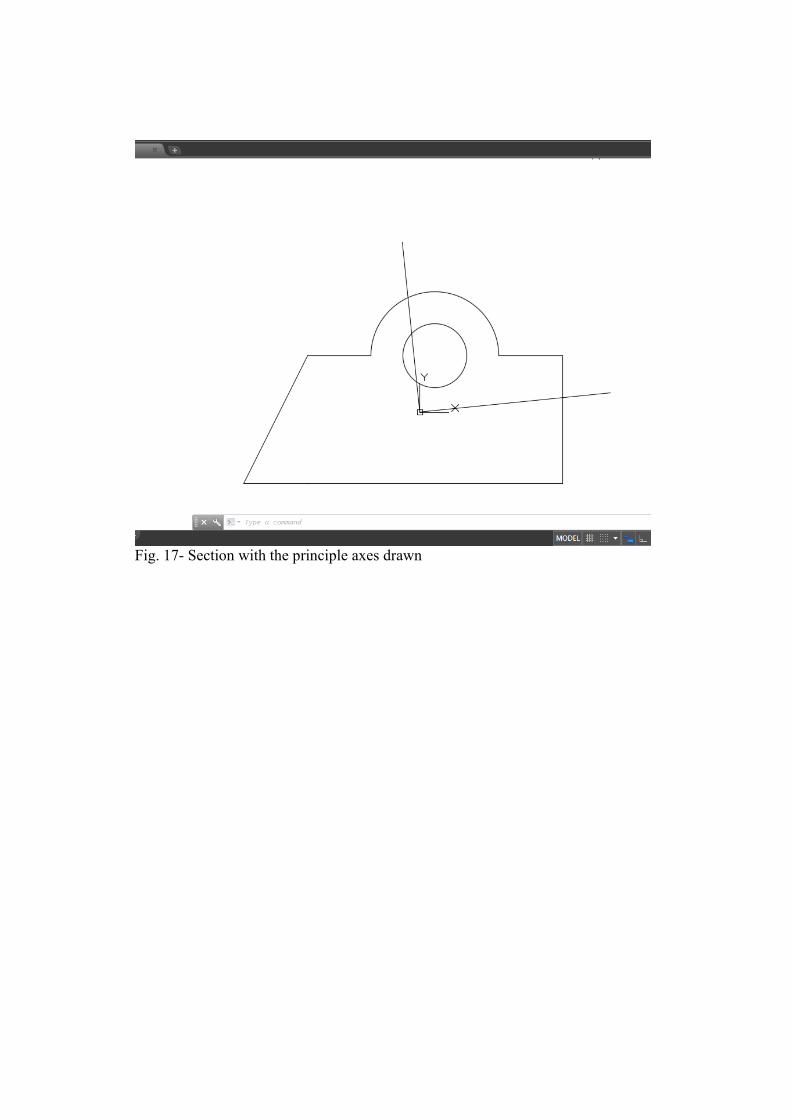
Fig. 17- Section with the principle axes drawn

Example 4: Using Auto Lisp to automate AutoCAD tasks Auto Lisp is a programing language used inside AutoCAD that can automate many tasks and make the work more productive. Many Auto Lisp programs are found in the Web to automate many tasks. Many of these problems are free to download and use. In the following examples some Auto Lisp commands will be explained.

All Auto Lisp commands consist of the following “ ( Command ……parameters)” for example to store a number e.g. 5.5 in a parameter R we use the command setq, the Auto Lisp command will look like this ( setq R 5.5) , it means let R be equal 5.5 Afterwards R can be used in any AutoCAD command instead of typing 5.5

Storing a value: In AutoCAD type the command (setq R 5.5), the Enter, then type the command Circle, pick the center of the circle and then when asked for the radius type !R instead of a number and then press Enter. A circle will be drawn with radius 5.5 because this number was already stored in R. See Fig. 18.

Asking Input from the user In Auto Lisp you can ask an input form the user. You can ask the user to input a value or pick a point and stored it in a variable. For example you can ask the user to enter a value for the radius of a circle and then store this value for later use. This can be done as follows: (setq R (getreal “\n Please input Radius value” ) ) The following command will ask the user to pick a point and will store in a variable called P1 (setq P1 (getpoint “\n Please pick a point” ) ) The message in both statement can be any text.

Using AutoCAD Commands in Auto Lisp Any AutoCAD command can be used in an auto lisp statement using the command word. For example, to draw a circle with a center at point P1 [stored earlier] with a radius R [stored earlier], the following Auto Lisp statement should be typed: (command “Circle” P1 R) A circle with center P1 and radius R will be drawn.

Using Calculations in Auto Lisp To draw a circle with a center P1 and radius R+20 the following statement can be typed (command “Circle” P1 (+ R 20 ) )

To draw a circle with a center P1 and radius 2R the following statement can be typed (command “Circle” P1 (* R 2 ) )

The above Auto Lisp statements can be combined to draw a group of co-centric circles as follows:

This function defines a new command called C1 that when typed will ask the user for a center point, a radius and a number n, then it will draw a n circles with increasing radii as shown in Fig. 19

Another version of the lisp program is shown below it does exactly the same function but also calculates and prints the area of each drawn circle and at the end it calculates and prints the sum of all Areas.

The lisp program can be typed directly in AutoCAD or can be saved in a file

and loaded in AutoCAD using Appload command. After the program is loaded a new command C1 will defined in AutoCAD that will run the above lisp program.

There are many free Auto Lisp programs in the web that can automate tasks and perform calculations.

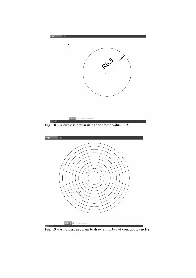
Fig. 18 – A circle is drawn using the stored value in R

Fig. 19 – Auto Lisp program to draw a number of concentric circles

 

 

 

MS Excel 

   

Civil Engineering Computer Application – MS Excel Second Year Civil

Solution of part b:

1) Open the MS Excel program. A new file is Opened by default. From the Menu Choose File-> Save As and save the file to the name “CA_5.xls”. 2) The Excel page is divided into cells. Each cell is defined by its row number and

column number. For Example cell E4 is the cell in Row no. 4 and Column no. E. To type any thing in the cell just click on the cell using the mouse, then starting typing.

3) Go To cell A4 and type the title Calculation of Area of Excavation. Go to the upper toolbar, and change the Font Size to 18, and choose B and U (Bold and Underlined)

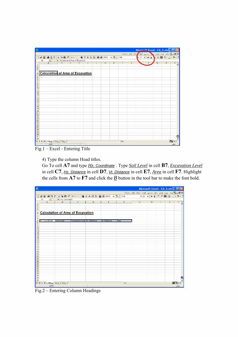
Fig.1 – Excel - Entering Title

4) Type the column Head titles. Go To cell A7 and type Hz. Coordinate . Type Soil Level in cell B7, Excavation Level in cell C7, Hz. Distance in cell D7, Vt. Distance in cell E7, Area in cell F7. Highlight the cells from A7 to F7 and click the B button in the tool bar to make the font bold.

Fig.2 – Entering Column Headings

5) In Column A Start at cell A8 and type the X coordinates from the table given in the problem. Similarly Type the Soil levels in Column B starting at B8, and the Excavation Levels at Column C starting at C8. 6) Type 1 in cells D8 and D18. Type 2 in cell D9, then press the Ctrl Button in the keyboard while typing C “Ctrl+C”. Select the cells from D10 to D17, and Press “Ctrl+V” to copy the value 2 in the selected cells.

Fgi.3 – Entering input information 7) To calculate the area of excavation the cross section is divided into equal strips of width 2 m each, except the first and last point with a strip of 1 m. the width of the strips were typed in the previous step in Column D. Column E is used to calculate the vertical distance at each strip ( the difference between the soil level and excavation level at the strip). Then Column F is used to calculate the area of excavation for the strip by multiplying the vertical distance of excavation by the strip width. 8) To do the calculations explained in the previous step, type the following in cell E8 =B8-C8 , then in cell F8 type =E8*D8. 9) To repeat the same calculations for all the strips, select cells E8 -> F8, and press “Ctrl+C”, then select cells E9 -> F18, and Press “Ctrl+V” to copy the equations to the selected cells. At this point the program has calculated the areas for all the strips, as shown in the following figure.

Fig.4 – Entering calculation formulas 10) To calculate the area of excavation obtain the sum of areas for all the strips. In cell A20 type Total Area of Excavation , then in cell F20 type =sum(F8..F18) , the total area of excavation will be displayed in cell F20 as shown in the following Figure.

Fig. 5- Calculating Final Summation

Finding the properties of a cross-section (C.G., area and Inertia)

1- Open a new Excel File and go to cell A4. Enter the title of the problem Finding

the properties of a cross-section (C.G., area and Inertia) in a bold underlined style.

2- Obtain a copy of the above section and paste it in the Excel Sheet as shown in Fig.6. The purpose of the image is to clarify the title.

Fig. 6- Entering the title and the problem figure

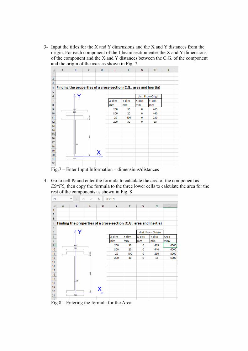
3- Input the titles for the X and Y dimensions and the X and Y distances from the origin. For each component of the I-beam section enter the X and Y dimensions of the component and the X and Y distances between the C.G. of the component and the origin of the axes as shown in Fig. 7.

Fig.7 – Enter Input Information – dimensions/distances

4- Go to cell I9 and enter the formula to calculate the area of the component as E9*F9, then copy the formula to the three lower cells to calculate the area for the rest of the components as shown in Fig. 8

Fig.8 – Entering the formula for the Area

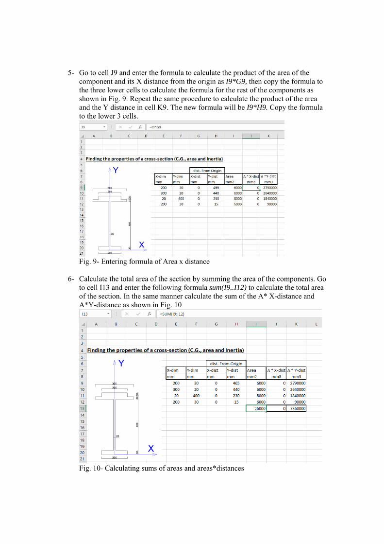
5- Go to cell J9 and enter the formula to calculate the product of the area of the component and its X distance from the origin as I9*G9, then copy the formula to the three lower cells to calculate the formula for the rest of the components as shown in Fig. 9. Repeat the same procedure to calculate the product of the area and the Y distance in cell K9. The new formula will be I9*H9. Copy the formula to the lower 3 cells.

Fig. 9- Entering formula of Area x distance

6- Calculate the total area of the section by summing the area of the components. Go to cell I13 and enter the following formula sum(I9..I12) to calculate the total area of the section. In the same manner calculate the sum of the A* X-distance and A*Y-distance as shown in Fig. 10

Fig. 10- Calculating sums of areas and areas*distances

7- To calculate the location of the center of gravity, enter the formula J13/I13 in cell J15 to calculate the X coordinate of the C.G. and K13/I13 in K15 to calculate the Y coordinate of the C.G. as shown in Fig. 11

Fig. 11- Calculate the C.G. coordinate of the section

8- The inertia of each component of the section is calculated as the sum of the inertia about the centroid of the component and the area of the component multiplied by the distance between the C.G. of the component and the C.G. of the section. The total inertia is calculated as the sum of the inertia of the components. This process is done for each of the X and Y directions as shown in Fig. 12.

To do that the distance between the C.G. of the component and C.G. of the section is calculated for the X and Y directions in columns L and M. In cell L9 enter the formula G9-$J$15 to calculate (X-Xo). In cell M9 enter the formula H9-$J$15 to calculate (Y-Yo). Copy the formulas to the lower cells to calculate for the rest of the components.

The inertia about the C.G. of each component is calculated for the X and Y directions in columns N and O for the X and Y directions, respectively. Ixo= Dx*Dy3 / 12 where Dx is the dimension in the x direction and Dy is the dimension in the y direction. The formulas for these calculations for the first component are (E9*F9^3)/12 to calculate Ixo and (F9*E9^3)/12 to calculate Iyo. The formulas should be copied to the lower cells for the rest of the components.

The inertia of the components about the main C.G. of the section is calculated as Ix= Ixo+ A* (x-xo)2 and as Iy= Iyo+ A* (y-yo)2. This is done in columns P and Q. The formulas for the first components are N9+I9*M9^2 for calculating Ix in cell P9 and O9+I9*L9^2 fro calculating Iy in cell Q9. The formulas are copied to the lower cells for the rest of the components.

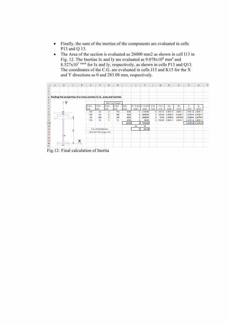
Finally, the sum of the inertias of the components are evaluated in cells P13 and Q 13.

The Area of the section is evaluated as 26000 mm2 as shown in cell I13 in Fig. 12. The Inertias Ix and Iy are evaluated as 9.078x108 mm4 and 8.527x107 mm4 for Ix and Iy, respectively, as shown in cells P13 and Q13. The coordinates of the C.G. are evaluated in cells J15 and K15 for the X and Y directions as 0 and 283.08 mm, respectively.

Fig.12- Final calculation of Inertia

 

 

 

SAP2000 

   

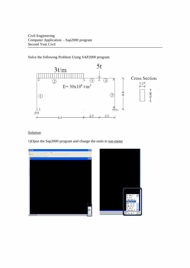
Civil Engineering Computer Application - Sap2000 program Second Year Civil Solve the following Problem Using SAP2000 program

Solution: 1)Open the Sap2000 program and change the units to ton-meter

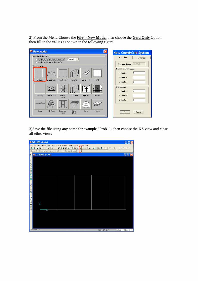
2) From the Menu Choose the File-> New Model then choose the Grid Only Option then fill in the values as shown in the following figure

3)Save the file using any name for example “Prob1” , then choose the XZ view and close all other views

4) Define the material property “E = 30 x 106 “ From the Menu Choose Define-> Materials then click the Add New Material buttton. Fill the Material Name Box with any name of your choice for Example “M1” and fill the Modulus of Elasticity Box with the given value 30x106 .

5) Define the section property as a rectangular section 0.25 x 0.60 . From the Menu Choose Define-> Frame/Cable Sections then choose Add Rectangle from the list down box, then click the Add New Property buttton. Fill the Sectionl Name Box with any name of your choice for Example “R25X60” and choose the Material “M1” defined in the previous step from the Material Box , then fill the values for the depth and width as 0.6 and 0.25 respectively as shown in the following figure.

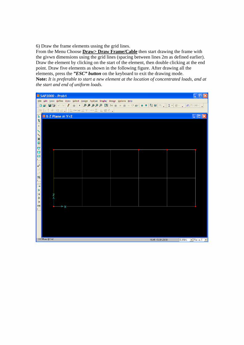
6) Draw the frame elements ussing the grid lines. From the Menu Choose Draw> Draw Frame/Cable then start drawing the frame with the givwn dimensions using the grid lines (spacing between lines 2m as defined earlier). Draw the element by clicking on the start of the element, then double clicking at the end point. Draw five elements as shown in the following figure. After drawing all the elements, press the ”ESC” button on the keyboard to exit the drawing mode. Note: It is preferable to start a new element at the location of concentrated loads, and at the start and end of uniform loads.

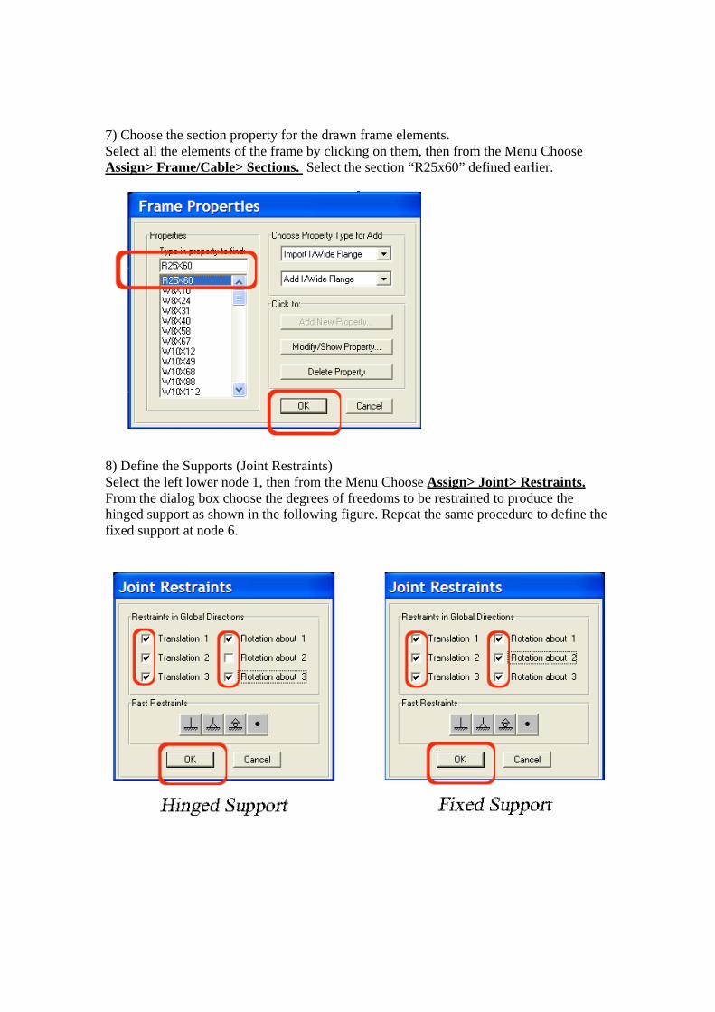
7) Choose the section property for the drawn frame elements. Select all the elements of the frame by clicking on them, then from the Menu Choose Assign> Frame/Cable> Sections. Select the section “R25x60” defined earlier.

8) Define the Supports (Joint Restraints) Select the left lower node 1, then from the Menu Choose Assign> Joint> Restraints. From the dialog box choose the degrees of freedoms to be restrained to produce the hinged support as shown in the following figure. Repeat the same procedure to define the fixed support at node 6.

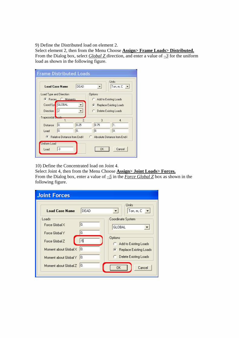
9) Define the Distributed load on element 2. Select element 2, then from the Menu Choose Assign> Frame Loads> Distributed. From the Dialog box, select Global Z direction, and enter a value of –3 for the uniform load as shown in the following figure.

10) Define the Concentrated load on Joint 4. Select Joint 4, then from the Menu Choose Assign> Joint Loads> Forces. From the Dialog box, enter a value of –5 in the Force Global Z box as shown in the following figure.

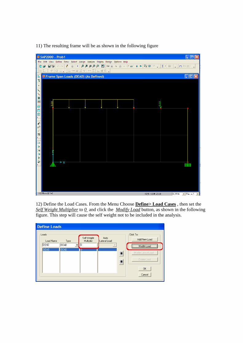
11) The resulting frame will be as shown in the following figure

12) Define the Load Cases. From the Menu Choose Define> Load Cases , then set the Self Weight Multiplier to 0 and click the Modify Load button, as shown in the following figure. This step will cause the self weight not to be included in the analysis.

13) From the Menu Choose Define > Analysis Cases , then delete all the analyses cases except the Linear Static Case. To delete an analysis case you need to Select the case and click the Delete Case Button as shown in the following figure.

14) From the Menu Choose Analyze> Run Analysis , then click Run Now Button to start solving the problem. After the analysis is complete, the deformed shape of the frame is displayed. Right click the mousse button at any joint to display the displacement values at that Joint, as shown in the following figure.

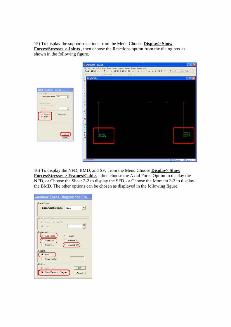
15) To display the support reactions from the Menu Choose Display> Show Forces/Stresses > Joints , then choose the Reactions option from the dialog box as shown in the following figure.

16) To display the NFD, BMD, and SF, from the Menu Choose Display> Show Forces/Stresses > Frames/Cables , then choose the Axial Force Option to display the NFD, or Choose the Shear 2-2 to display the SFD, or Choose the Moment 3-3 to display the BMD. The other options can be chosen as displayed in the following figure.

 

 

 

CIVIL 3D 

Introduction to Civil 3D

Unit one: Points

Introduction

The foundation of any civil engineering project is the simple point, frequently referred to

as shots. Most commonly, points are used to identify the location of existing features, such

as trees and property corners; topography, such as ground shots; or stakeout information,

such as road geometry points. However, points can be used for much more. This chapter

will both focus on traditional point uses and introduce ideas to apply the dynamic power

of point editing, labeling, and grouping to other applications.

In this chapter, you will learn to:

Import points from a text file using description

Create a point group

Create a point table

Anatomy of a Point

Civil 3D points (see Figure 1) are intelligent objects that represent x, y, and z locations in

space. Each point has a unique number and, optionally, a unique name that can be used for

additional identification and labeling.

 

 

 

 

 

 

 

 

 

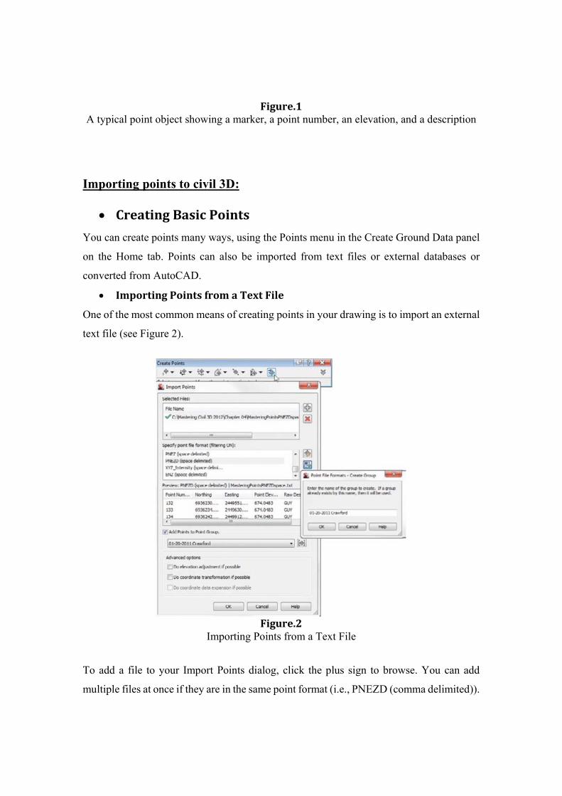
Figure.1A typical point object showing a marker, a point number, an elevation, and a description

Importing points to civil 3D:

CreatingBasicPoints

You can create points many ways, using the Points menu in the Create Ground Data panel

on the Home tab. Points can also be imported from text files or external databases or

converted from AutoCAD.

ImportingPointsfromaTextFile

One of the most common means of creating points in your drawing is to import an external

text file (see Figure 2).

Figure.2

Importing Points from a Text File

To add a file to your Import Points dialog, click the plus sign to browse. You can add

multiple files at once if they are in the same point format (i.e., PNEZD (comma delimited)).

The import process supports most text formats as well as Microsoft Access Database

(MDB) files.

When your file is listed in the top of the dialog box, a green check mark will indicate that

Civil 3D can parse the information. Be careful, though, as Civil 3D does not know the

difference between a Northing and an Easting or a point number and an elevation. You still

need to select the correct file format.

The file format filter is there to help you. Civil 3D recognizes how the file is delimited (i.e.,

tab, comma, space) and only shows you the formats that apply. If you don’t want the help,

you can turn the filtering off by clicking the Filter icon.

The importing text file of points can be abbreviated in the following steps:

1. Open the Import Points dialog by selecting Points from File in the Import panel of the

Insert tab.

2. Change the Format field to PNEZD (Comma Delimited).

3. Click the file folder’s plus (+) button to the right of the Source File field, and navigate

out to locate the Points.txt file.

4. Click the Create Point group icon. Name the point group Survey and click OK.

5. Leave all the other boxes unchecked.

6. Click OK. You may have to use Zoom Extents to see the imported points.

PointGroups:

Working with point groups is one of the most powerful techniques you will learn. Want to

turn all your points off without touching layers? Make a point group! Want to move last

week’s survey up by the blown instrument height difference? Make a point group!

Want to prevent invert shots from throwing off your surface model? Point group! Point

group!

A point group is a collection of points that has been filtered for a certain criterion. You can

use any property of the points, such as description, elevation, and point number, or you can

select points in the drawing.

Civil 3D creates the _All Points group for you, which contains every point in the drawing.

It cannot be renamed, deleted, or have its properties modified to exclude any points. Create

point groups for a collection of points you might wish to separate from others, as shown in

Figure 3.

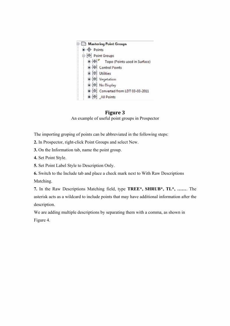
Figure3An example of useful point groups in Prospector

The importing groping of points can be abbreviated in the following steps:

2. In Prospector, right-click Point Groups and select New.

3. On the Information tab, name the point group.

4. Set Point Style.

5. Set Point Label Style to Description Only.

6. Switch to the Include tab and place a check mark next to With Raw Descriptions

Matching.

7. In the Raw Descriptions Matching field, type TREE*, SHRUB*, TL*, ……. The

asterisk acts as a wildcard to include points that may have additional information after the

description.

We are adding multiple descriptions by separating them with a comma, as shown in

Figure 4.

Figure4

The point group dialog box.

Unit two: Surfaces

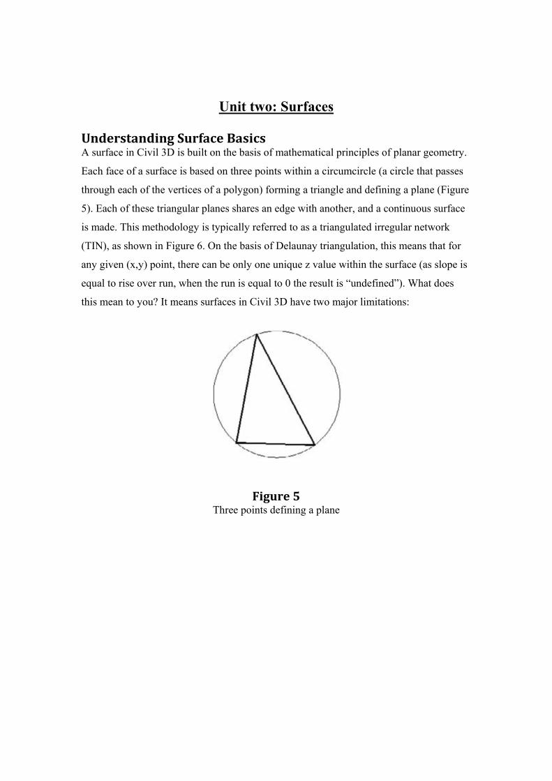
UnderstandingSurfaceBasicsA surface in Civil 3D is built on the basis of mathematical principles of planar geometry.

Each face of a surface is based on three points within a circumcircle (a circle that passes

through each of the vertices of a polygon) forming a triangle and defining a plane (Figure

5). Each of these triangular planes shares an edge with another, and a continuous surface

is made. This methodology is typically referred to as a triangulated irregular network

(TIN), as shown in Figure 6. On the basis of Delaunay triangulation, this means that for

any given (x,y) point, there can be only one unique z value within the surface (as slope is

equal to rise over run, when the run is equal to 0 the result is “undefined”). What does

this mean to you? It means surfaces in Civil 3D have two major limitations:

Figure5Three points defining a plane

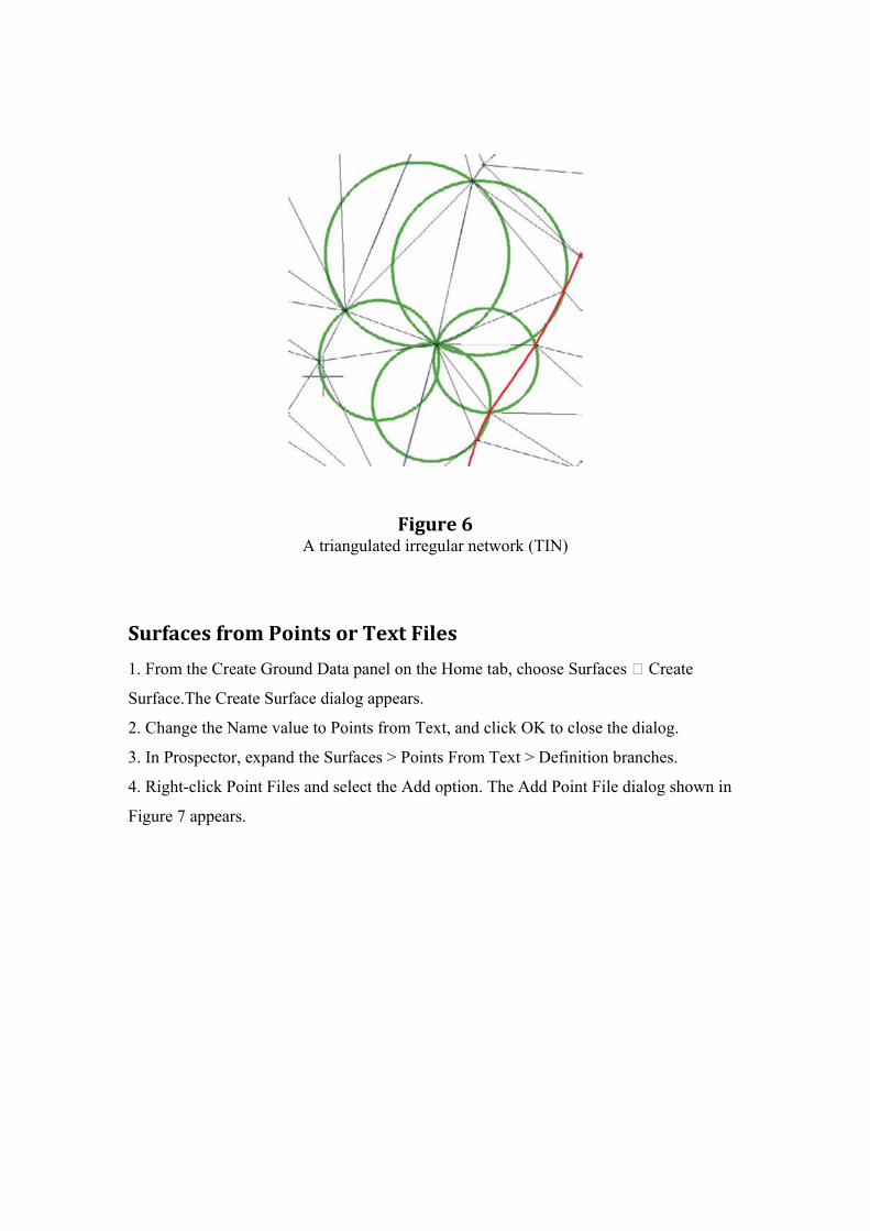
Figure6A triangulated irregular network (TIN)

SurfacesfromPointsorTextFiles

1. From the Create Ground Data panel on the Home tab, choose Surfaces Create

Surface.The Create Surface dialog appears.

2. Change the Name value to Points from Text, and click OK to close the dialog.

3. In Prospector, expand the Surfaces > Points From Text > Definition branches.

4. Right-click Point Files and select the Add option. The Add Point File dialog shown in

Figure 7 appears.

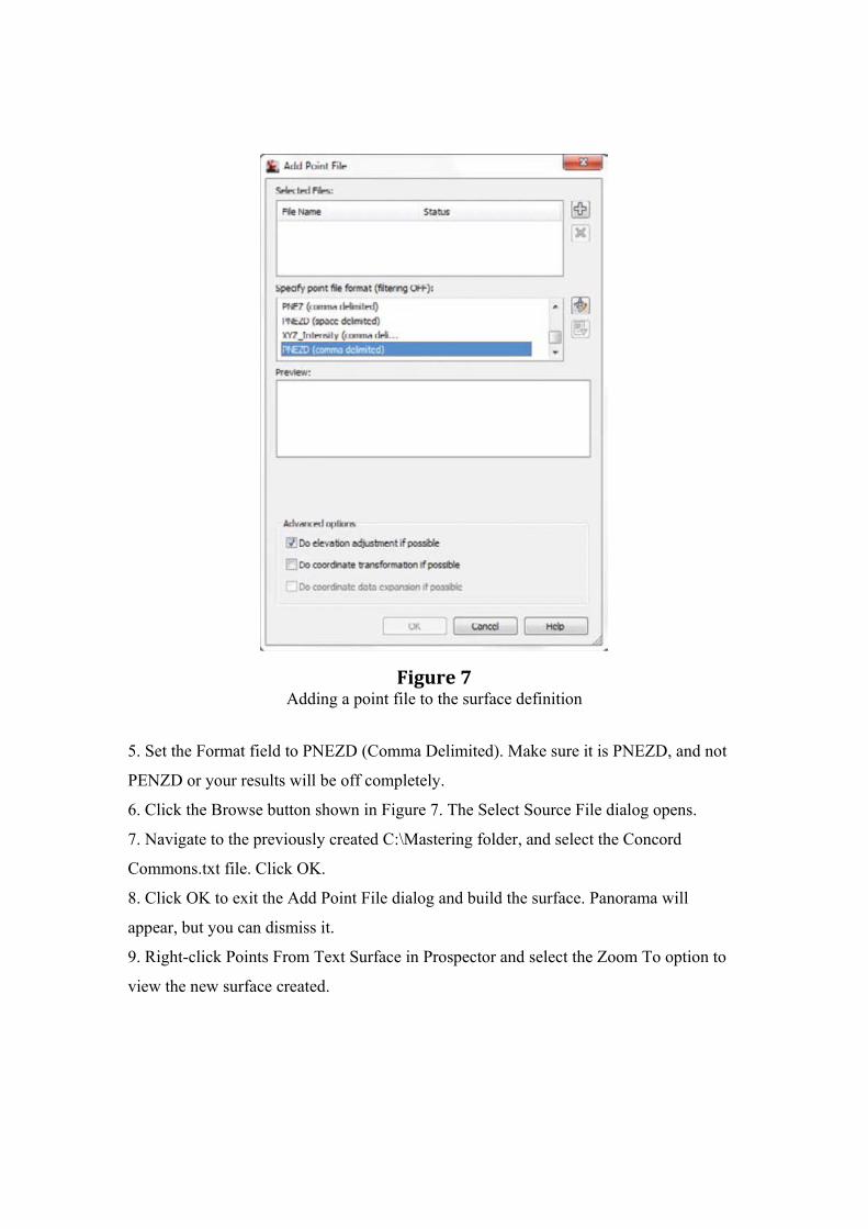
Figure7Adding a point file to the surface definition

5. Set the Format field to PNEZD (Comma Delimited). Make sure it is PNEZD, and not

PENZD or your results will be off completely.

6. Click the Browse button shown in Figure 7. The Select Source File dialog opens.

7. Navigate to the previously created C:\Mastering folder, and select the Concord

Commons.txt file. Click OK.

8. Click OK to exit the Add Point File dialog and build the surface. Panorama will

appear, but you can dismiss it.

9. Right-click Points From Text Surface in Prospector and select the Zoom To option to

view the new surface created.

RefiningandEditingSurfaces

Once a basic surface is built, and, in some cases, even before it is built, you can do some

cleanup and modification to the TIN construction that make it much more usable and

realistic. Some of these edits include limiting the input data, tweaking the triangulation,

adding in breakline information, or hiding areas from view. In this section, we explore a

number of ways of refining surfaces to end up with the best possible model from which to

build.

SurfaceProperties

The most basic steps you can perform in making a better model are right in the Surface

Properties dialog. The surface object contains information about the build and edit

operations, along with some values used in surface calculations. These values can be used

to tweak your surface to a semi-acceptable state before more manual operations are needed.

In this exercise, you’ll go through a couple of the basic surface-building controls that are

available.

You’ll do them one at a time in order to measure their effects on the final surface

display.

1. Open the DWG file. This is the Points From Text drawing that you worked on earlier.

2. Expand the Surfaces branch.

3. Right-click EG and select Surface Properties. The Surface Properties dialog appears.

4. Select the Definition tab. Note the list at the bottom of the dialog.

5. Under the Definition Options at the top of the dialog, expand the Build option.

PointandTriangleEditing

In this section, you’ll remove triangles manually, and then finish your surface by

correcting what appears to be a blown survey shot.

1. In Prospector, expand the Surfaces > EG > Definition branches.

2. Right-click Edits and select the Delete Line option.

3. Enter C as the command line to enter a crossing selection mode.

4. Start at the lower right of the pick area shown in Figure 8, and move to the upper-left

corner as shown. Right-click or press ↵ to finish the selection.

5. Repeat this process, removing triangles until your site resembles Figure 9.

6. Zoom to the portion of your site with the red circle, and you’ll notice a collection of

contours that seems out of place.

7. Change Surface Style to Contours and Points.

Figure8Crossing the window selection to delete TIN lines

Figure9Surface after removal of extraneous triangles

            Al‐Azhar University             College of Engineering 

Civil Engineering Department                      Computer Applications                     Second Year 

١  

GMS SEEP2D program SEEP2D is a two-dimensional finite element program used to produce 2D groundwater profile models such as cross-sections of earth dams or levees. SEEP2D can be used for either confined or unconfined steady state flow models. For unconfined models, both saturated and unsaturated flow is simulated. A variety of options are provided in GMS for displaying SEEP2D results. Contours of total head (equipotential lines) and flow vectors can be plotted. An option is also available for computing flow potential values at the nodes. These values can be used to plot flow lines. Together with the equipotential lines (lines of constant total head), the flow lines can be used to plot a flow net.

Example problem

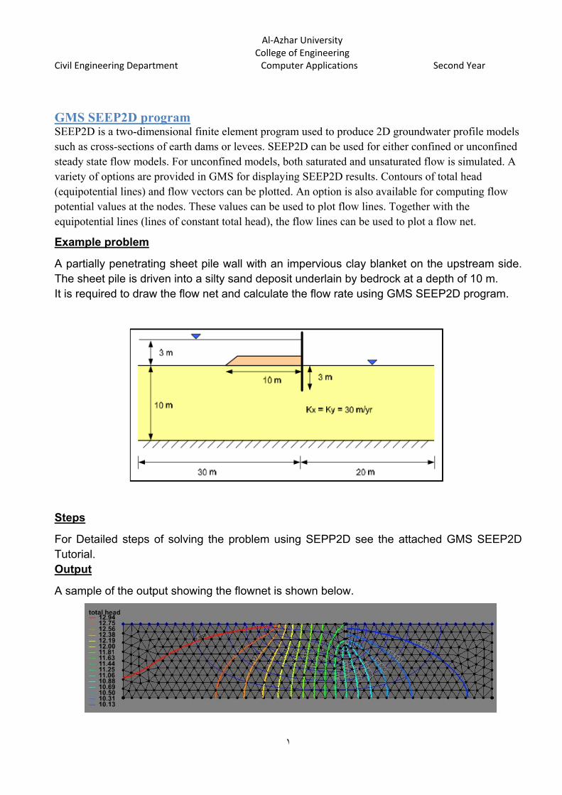
A partially penetrating sheet pile wall with an impervious clay blanket on the upstream side. The sheet pile is driven into a silty sand deposit underlain by bedrock at a depth of 10 m. It is required to draw the flow net and calculate the flow rate using GMS SEEP2D program.

Steps

For Detailed steps of solving the problem using SEPP2D see the attached GMS SEEP2D Tutorial. Output

A sample of the output showing the flownet is shown below.