axial compressor - weebly
TRANSCRIPT
CFD Final Project 2017
Axial Compressor
Team #5 Qing Xu, Arvinth Sethuraman, Abraham Tawil,
MingYang Lee, Mizanur Rahman
Design Time Estimate 200 hours
Problem Statement We were asked to design the compressor stage for a new type of gas turbofan engine. The
axial compressor will be used to increase the density of intake air before it is fed into a combustor. The performance requirements required a minimum pressure ratio of 18:1 at the maximum working altitude of 40,000 ft. Additionally, the design constraints were a maximum operating speed of 85,000 rpm for any stage, and the outer diameter of the compressor to be between 4 ft. and 6 ft. Because physical prototyping would result in too high a cost, and a lot of design variables are included (blade geometry, angle of attack, compressor tapering effect, etc.), CFD is a good tool to help the design process and validate the reasonability of design decisions. Design Assumptions
For the purpose of this simulation, it was assumed that the compressor was operated on a test stand, and the entrance flow was at subsonic speeds. The temperature and pressure conditions are assumed to be at the standard conditions for atmospheric air at each respective altitude (in this case, 40,000 ft altitude and at sea level). The density of the air was modeled as that of an ideal gas. Design Concept & Compressor Geometry
Based on research on the design of existing axial compressors, we decided that a multi-stage axial compressor will be most suitable for the problem imposed. A single stage compressor will fail to provide high efficiency, and more importantly not fulfill the design requirement of 1:18 pressure ratio given the geometry constraint. Each stage of the compressor consists of one rotor and one stator. The air output of one stage will go into the next stage for further compression.
In a traditional design of axial compressor according to our online research, an extra section of stator is usually placed before the first section of rotor as inlet guilds, However, preliminary mixing plane simulation shows that the inlet guild will result in a unnecessary pressure loss. So even though from the perspective of safety the most exterior sections should not be rotating parts, the inlet guild section is not included in the compressor design. Extra layers of protections can be put outside for increasing safety factor.
For the purpose of helping air accelerate in the compressor, a tapering shape was used for the first stage of the compressor. The tapering geometry was achieved by tapering the shroud surface of the first stage, while keeping the core diameter constant.
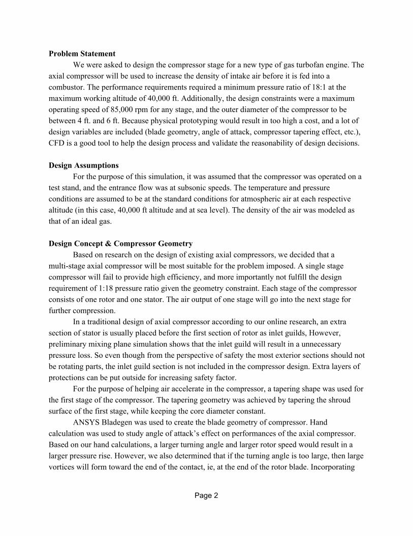
ANSYS Bladegen was used to create the blade geometry of compressor. Hand calculation was used to study angle of attack’s effect on performances of the axial compressor. Based on our hand calculations, a larger turning angle and larger rotor speed would result in a larger pressure rise. However, we also determined that if the turning angle is too large, then large vortices will form toward the end of the contact, ie, at the end of the rotor blade. Incorporating
Page 2
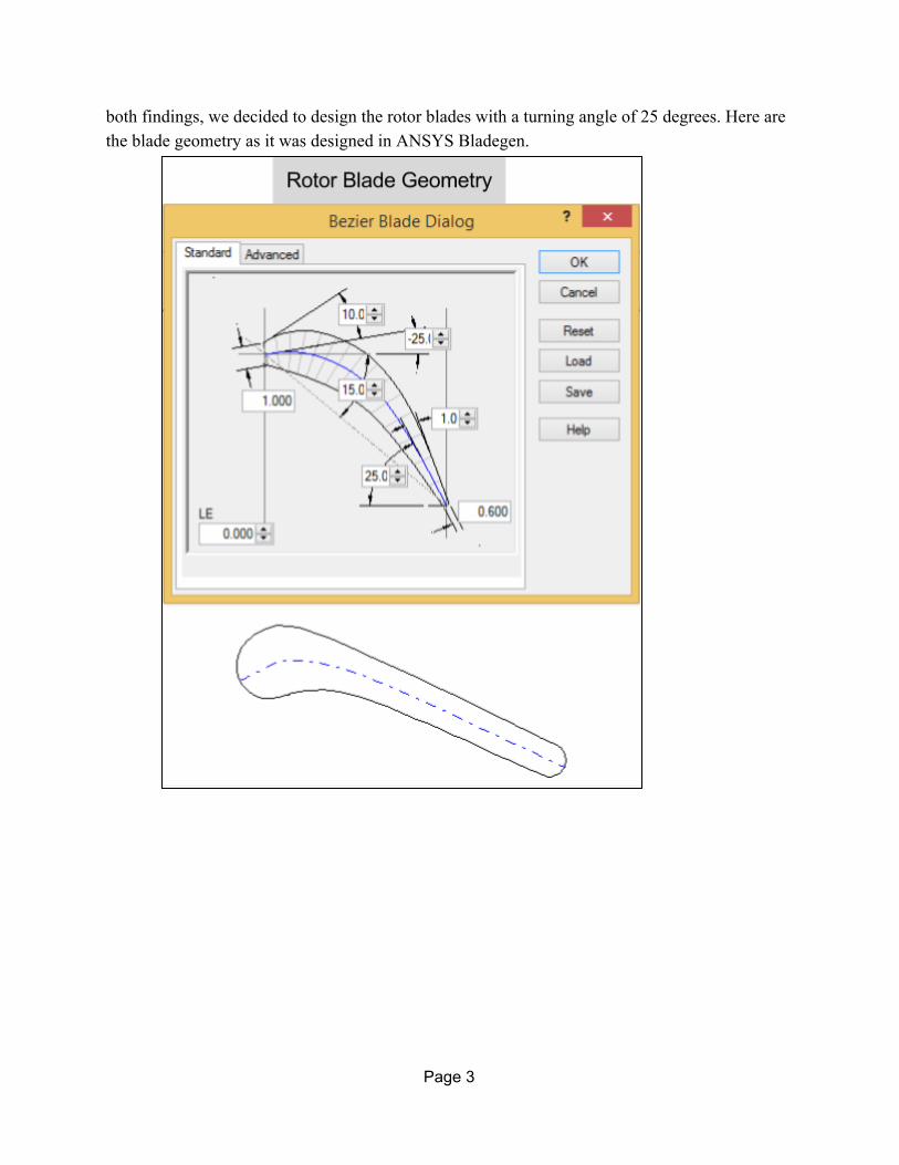
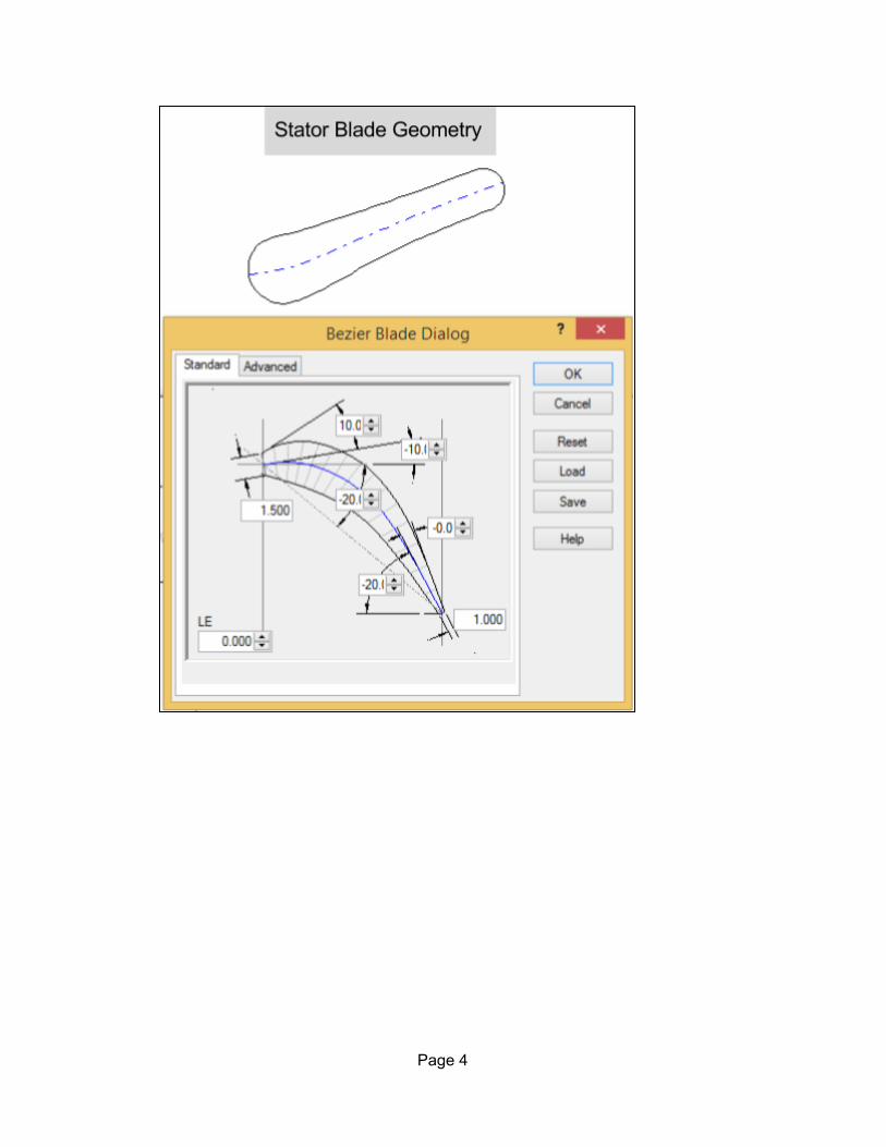
both findings, we decided to design the rotor blades with a turning angle of 25 degrees. Here are the blade geometry as it was designed in ANSYS Bladegen.
Page 3
Page 4
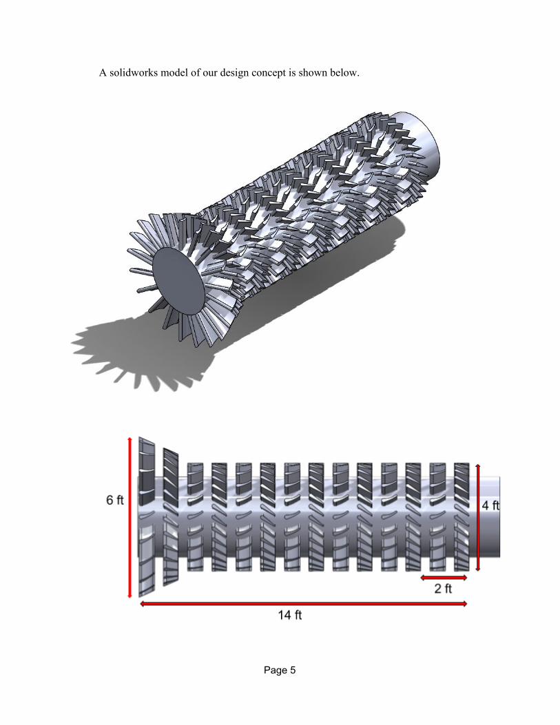
A solidworks model of our design concept is shown below.
Page 5

The compressor alternates between rotors and stators for a total of 7 stages (1 rotor
section and 1 stator section per stage). The length of each stage is 2 ft. Each of the rotor stages have 20 blades, and the stator sections contain 30 blades each. The initial stage is tapered to provide a reduction in area. The outer diameter of the compressor both before and after the taper is 6ft and 4 ft, respectively.
Summary of Compressor Geometry
Max Outer Diameter 6 ft
Min Outer Diameter 4 ft
Compressor Length 14 ft
Inner (Core) Diameter 3 ft
Page 6
Minimum Blade Length 0.5 ft
Maximum Blade Length 1.5 ft
Turning angle 25°
Rotor speed 3000 rpm
Number of Stages 20
Rotor Blades (per stage) 20
Stator Blades (per stage) 30
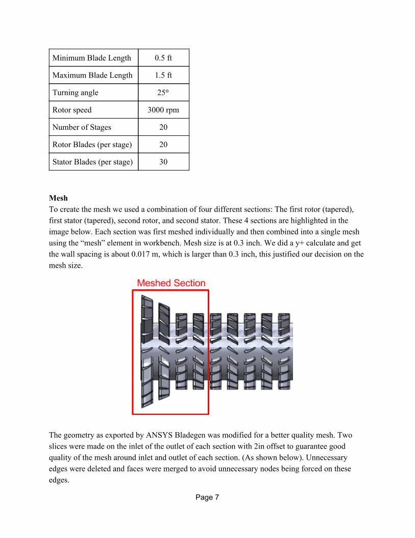
Mesh To create the mesh we used a combination of four different sections: The first rotor (tapered), first stator (tapered), second rotor, and second stator. These 4 sections are highlighted in the image below. Each section was first meshed individually and then combined into a single mesh using the “mesh” element in workbench. Mesh size is at 0.3 inch. We did a y+ calculate and get the wall spacing is about 0.017 m, which is larger than 0.3 inch, this justified our decision on the mesh size.
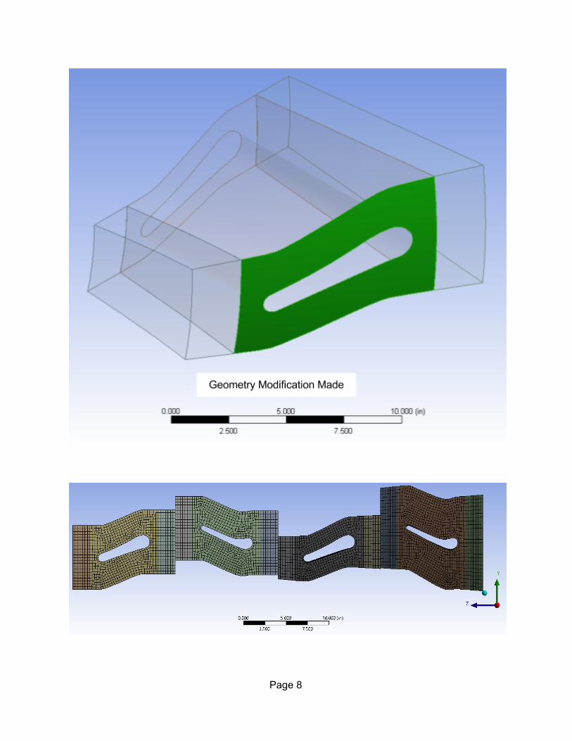
The geometry as exported by ANSYS Bladegen was modified for a better quality mesh. Two slices were made on the inlet of the outlet of each section with 2in offset to guarantee good quality of the mesh around inlet and outlet of each section. (As shown below). Unnecessary edges were deleted and faces were merged to avoid unnecessary nodes being forced on these edges.
Page 7
Page 8
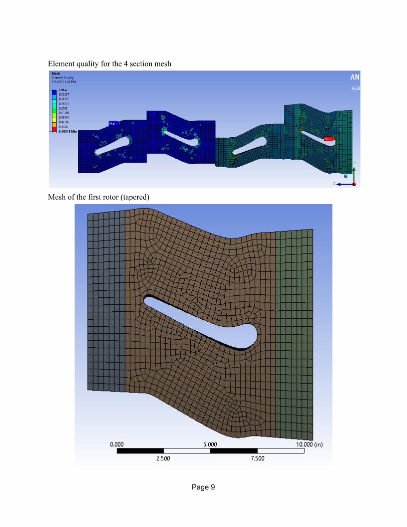
Element quality for the 4 section mesh
Mesh of the first rotor (tapered)
Page 9
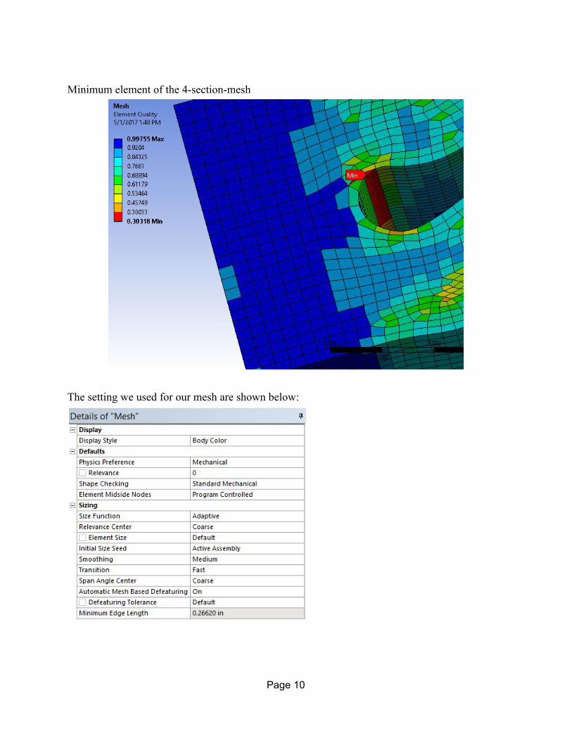
Minimum element of the 4-section-mesh
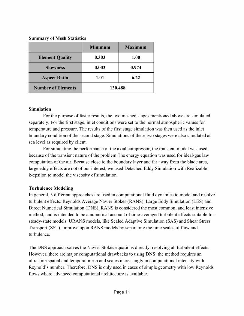
The setting we used for our mesh are shown below:
Page 10
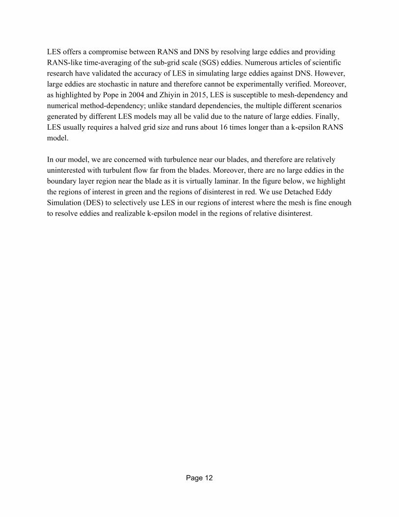
Summary of Mesh Statistics
Minimum Maximum
Element Quality 0.303 1.00
Skewness 0.003 0.974
Aspect Ratio 1.01 6.22
Number of Elements 130,488
Simulation
For the purpose of faster results, the two meshed stages mentioned above are simulated separately. For the first stage, inlet conditions were set to the normal atmospheric values for temperature and pressure. The results of the first stage simulation was then used as the inlet boundary condition of the second stage. Simulations of these two stages were also simulated at sea level as required by client.
For simulating the performance of the axial compressor, the transient model was used because of the transient nature of the problem.The energy equation was used for ideal-gas law computation of the air. Because close to the boundary layer and far away from the blade area, large eddy effects are not of our interest, we used Detached Eddy Simulation with Realizable k-epsilon to model the viscosity of simulation. Turbulence Modeling In general, 3 different approaches are used in computational fluid dynamics to model and resolve turbulent effects: Reynolds Average Navier Stokes (RANS), Large Eddy Simulation (LES) and Direct Numerical Simulation (DNS). RANS is considered the most common, and least intensive method, and is intended to be a numerical account of time-averaged turbulent effects suitable for steady-state models. URANS models, like Scaled Adaptive Simulation (SAS) and Shear Stress Transport (SST), improve upon RANS models by separating the time scales of flow and turbulence. The DNS approach solves the Navier Stokes equations directly, resolving all turbulent effects. However, there are major computational drawbacks to using DNS: the method requires an ultra-fine spatial and temporal mesh and scales increasingly in computational intensity with Reynold’s number. Therefore, DNS is only used in cases of simple geometry with low Reynolds flows where advanced computational architecture is available.
Page 11
LES offers a compromise between RANS and DNS by resolving large eddies and providing RANS-like time-averaging of the sub-grid scale (SGS) eddies. Numerous articles of scientific research have validated the accuracy of LES in simulating large eddies against DNS. However, large eddies are stochastic in nature and therefore cannot be experimentally verified. Moreover, as highlighted by Pope in 2004 and Zhiyin in 2015, LES is susceptible to mesh-dependency and numerical method-dependency; unlike standard dependencies, the multiple different scenarios generated by different LES models may all be valid due to the nature of large eddies. Finally, LES usually requires a halved grid size and runs about 16 times longer than a k-epsilon RANS model. In our model, we are concerned with turbulence near our blades, and therefore are relatively uninterested with turbulent flow far from the blades. Moreover, there are no large eddies in the boundary layer region near the blade as it is virtually laminar. In the figure below, we highlight the regions of interest in green and the regions of disinterest in red. We use Detached Eddy Simulation (DES) to selectively use LES in our regions of interest where the mesh is fine enough to resolve eddies and realizable k-epsilon model in the regions of relative disinterest.
Page 12

In theory, LES applies Kolmogorov’s 1941 theory that large eddies are geometrically dependent. Therefore, we can achieve LES by applying a convolutional filter kernel G on flow field u to generate a partially resolved flow field.
And then, we are able to appropriately adapt the Navier Stokes equations:
Kolmogorov microscales were also developed to determine the required temporal and spatial resolutions for resolving large eddies, as shown in the table below. Specifically at this scale, viscosity dominates flow and turbulent energy is mostly dissipated into heat. From initial simulations run with a standard k-epsilon RANS model, we input peak flow velocity and
Page 13
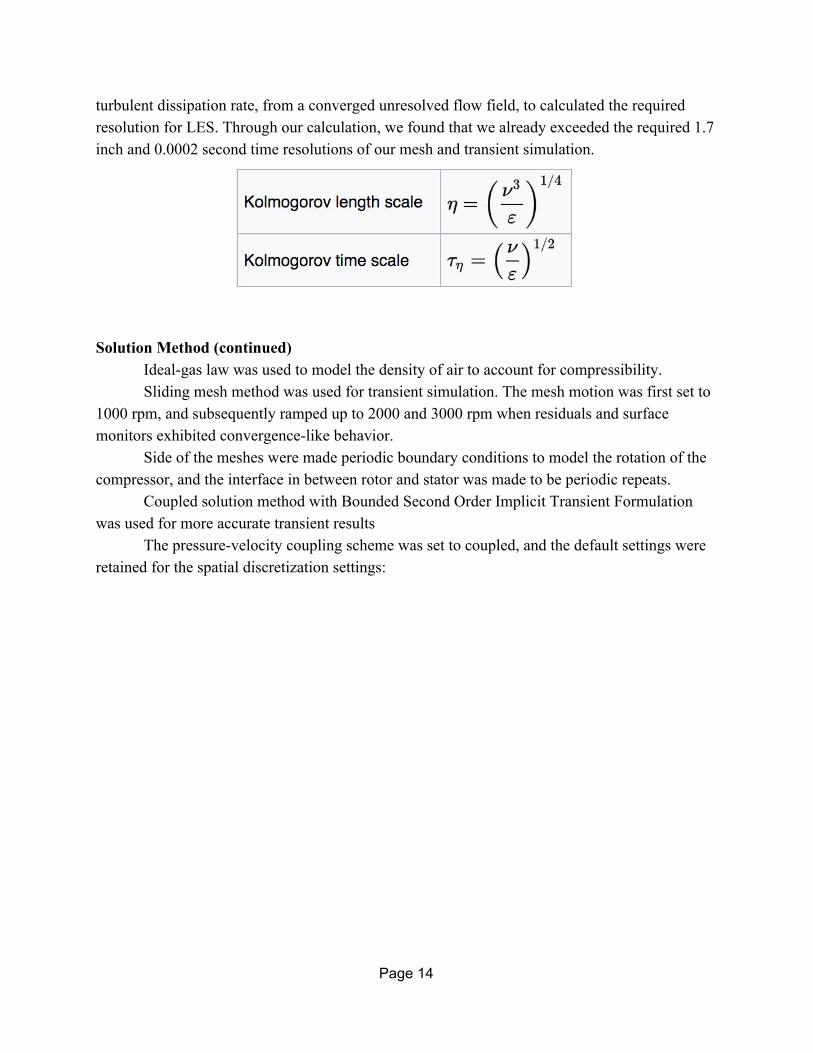
turbulent dissipation rate, from a converged unresolved flow field, to calculated the required resolution for LES. Through our calculation, we found that we already exceeded the required 1.7 inch and 0.0002 second time resolutions of our mesh and transient simulation.
Solution Method (continued)
Ideal-gas law was used to model the density of air to account for compressibility. Sliding mesh method was used for transient simulation. The mesh motion was first set to
1000 rpm, and subsequently ramped up to 2000 and 3000 rpm when residuals and surface monitors exhibited convergence-like behavior.
Side of the meshes were made periodic boundary conditions to model the rotation of the compressor, and the interface in between rotor and stator was made to be periodic repeats.
Coupled solution method with Bounded Second Order Implicit Transient Formulation was used for more accurate transient results
The pressure-velocity coupling scheme was set to coupled, and the default settings were retained for the spatial discretization settings:
Page 14

Page 15
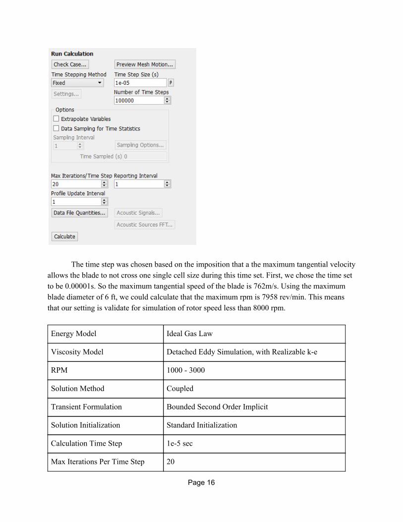
The time step was chosen based on the imposition that a the maximum tangential velocity allows the blade to not cross one single cell size during this time set. First, we chose the time set to be 0.00001s. So the maximum tangential speed of the blade is 762m/s. Using the maximum blade diameter of 6 ft, we could calculate that the maximum rpm is 7958 rev/min. This means that our setting is validate for simulation of rotor speed less than 8000 rpm.
Energy Model Ideal Gas Law
Viscosity Model Detached Eddy Simulation, with Realizable k-e
RPM 1000 - 3000
Solution Method Coupled
Transient Formulation Bounded Second Order Implicit
Solution Initialization Standard Initialization
Calculation Time Step 1e-5 sec
Max Iterations Per Time Step 20
Page 16
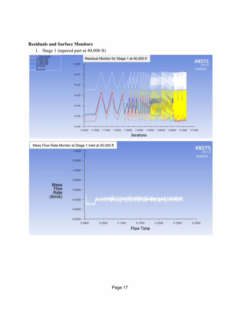
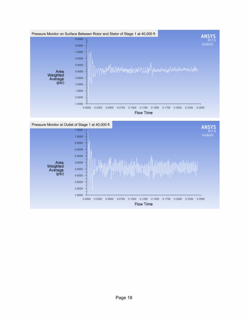
Residuals and Surface Monitors
1. Stage 1 (tapered part at 40,000 ft)
Page 17
Page 18

2. Stage 2 (flat stage at 40,000 ft)
Page 19

3. Stage 1 (tapered at sea level)
Page 20

Page 21

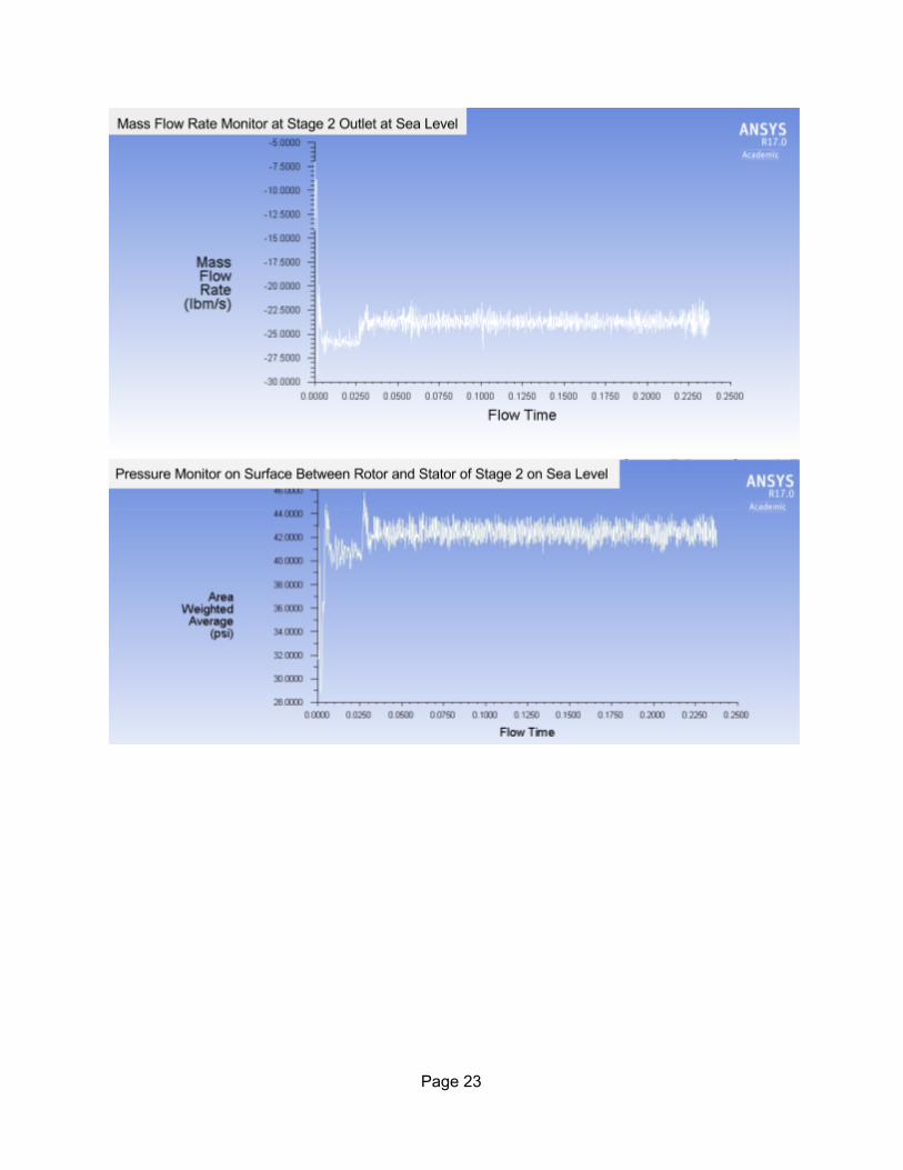
4. Stage 2 (flat at sea level)
Page 22
Page 23
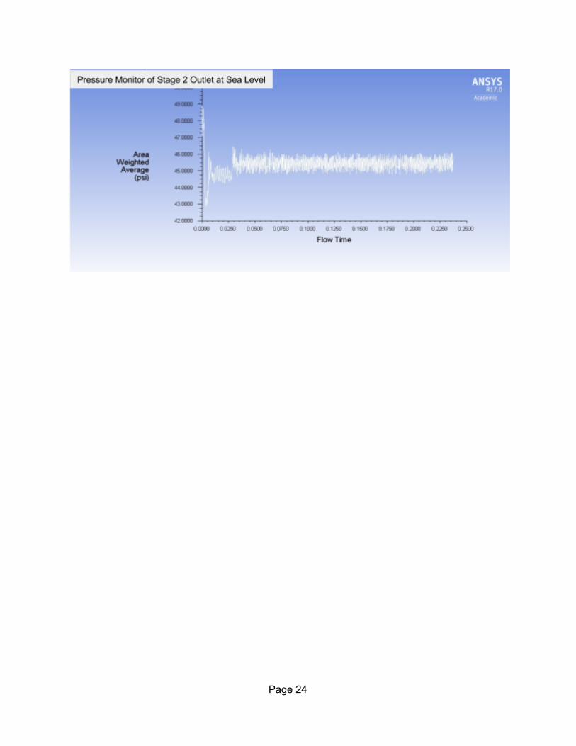
Page 24

Contour Plots of Simulated Results Compression Ratio
The compression ratio of the first stage at 40,000 ft altitude is 1.52. This can be
visualized on the plot above and is consistent with our hand calculation value of 1.57.
Page 25

The compression ratio of the second stage at 40,000 ft altitude is about 1.43. This can be
visualized from the plot above. Although there is a slight discrepancy between this value and the calculated compression ratio of 1.31, the two value agrees within an order of magnitude.
Page 26
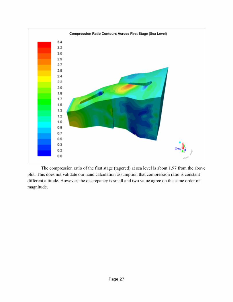
The compression ratio of the first stage (tapered) at sea level is about 1.97 from the above
plot. This does not validate our hand calculation assumption that compression ratio is constant different altitude. However, the discrepancy is small and two value agree on the same order of magnitude.
Page 27

The compression ratio of the second stage at sea level is 1.85. This is also slightly higher
than what we predict, but is is consist with the trend of the first stage that at sea level, compression ratio is slightly higher. Summarized Compression Ratios:
Stage Ratio at 40,000 ft Ratio at sea level
First 1.52 2
Second 1.43 1.85
Last 5* 1.43 1.85
*Should be decreasing stage by stage. Future work can be done to model these subsequent stages in more detail.
Page 28
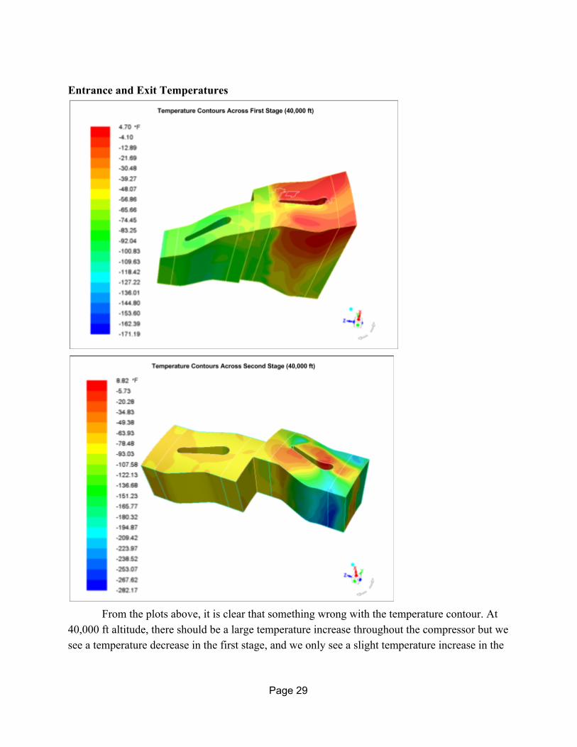
Entrance and Exit Temperatures
From the plots above, it is clear that something wrong with the temperature contour. At
40,000 ft altitude, there should be a large temperature increase throughout the compressor but we see a temperature decrease in the first stage, and we only see a slight temperature increase in the
Page 29
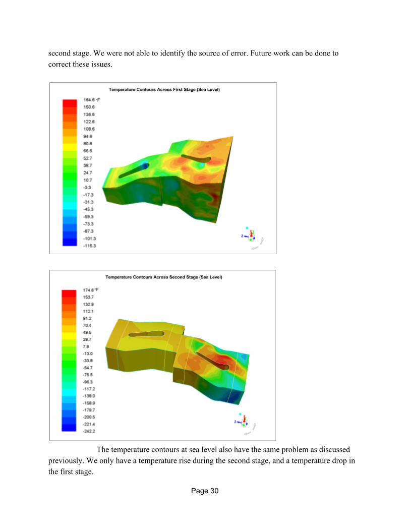
second stage. We were not able to identify the source of error. Future work can be done to correct these issues.
The temperature contours at sea level also have the same problem as discussed
previously. We only have a temperature rise during the second stage, and a temperature drop in the first stage.
Page 30

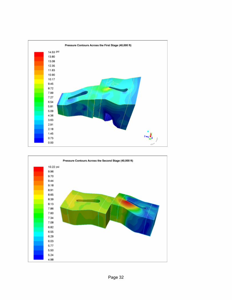
Pressure Contours
Page 31
Page 32
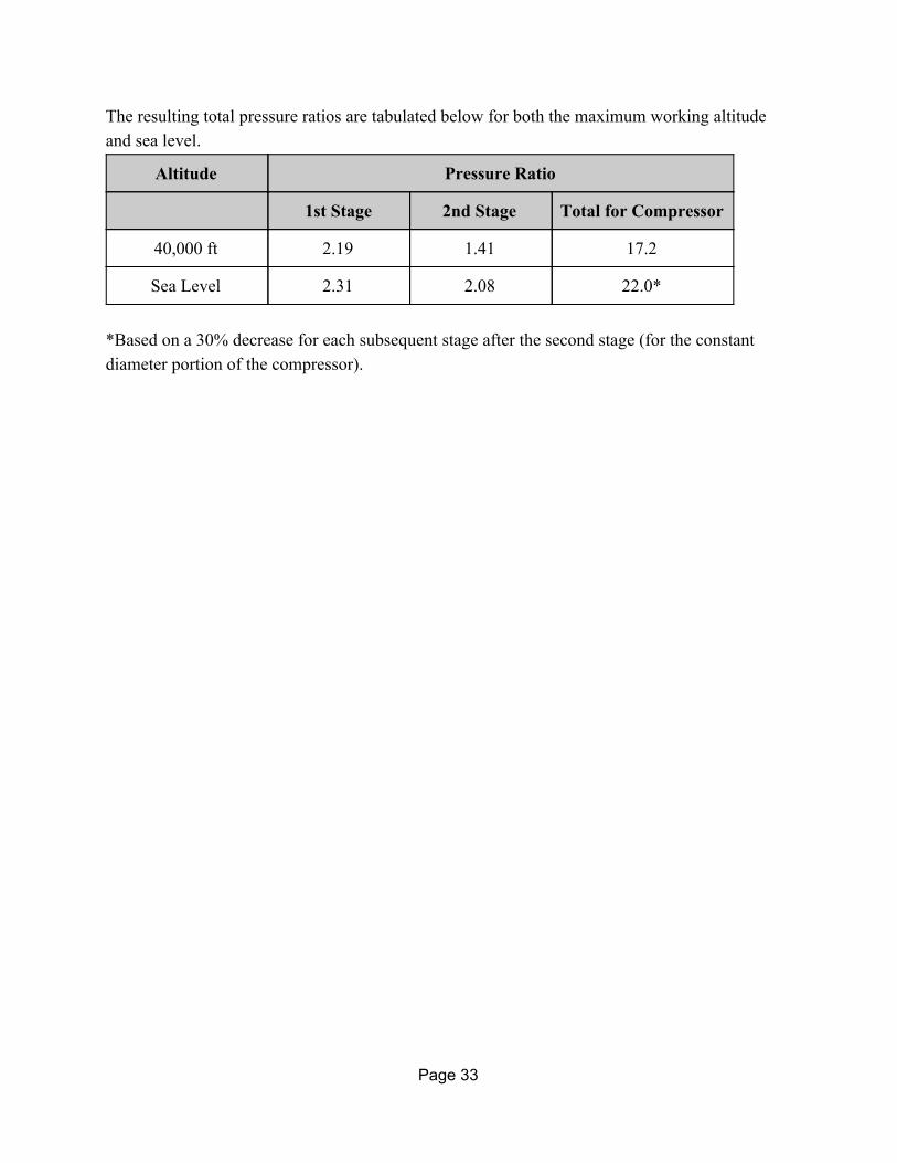
The resulting total pressure ratios are tabulated below for both the maximum working altitude and sea level.
Altitude Pressure Ratio
1st Stage 2nd Stage Total for Compressor
40,000 ft 2.19 1.41 17.2
Sea Level 2.31 2.08 22.0*
*Based on a 30% decrease for each subsequent stage after the second stage (for the constant diameter portion of the compressor).
Page 33
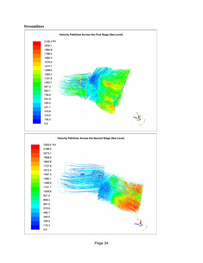
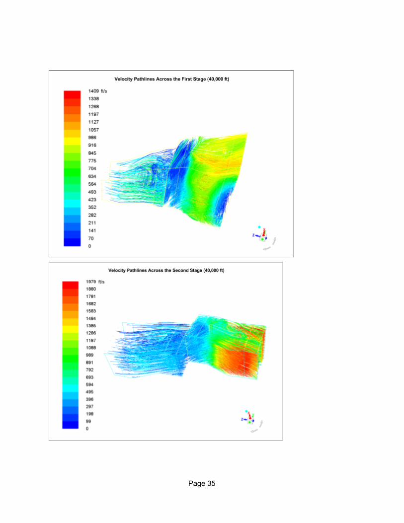
Streamlines
Page 34
Page 35
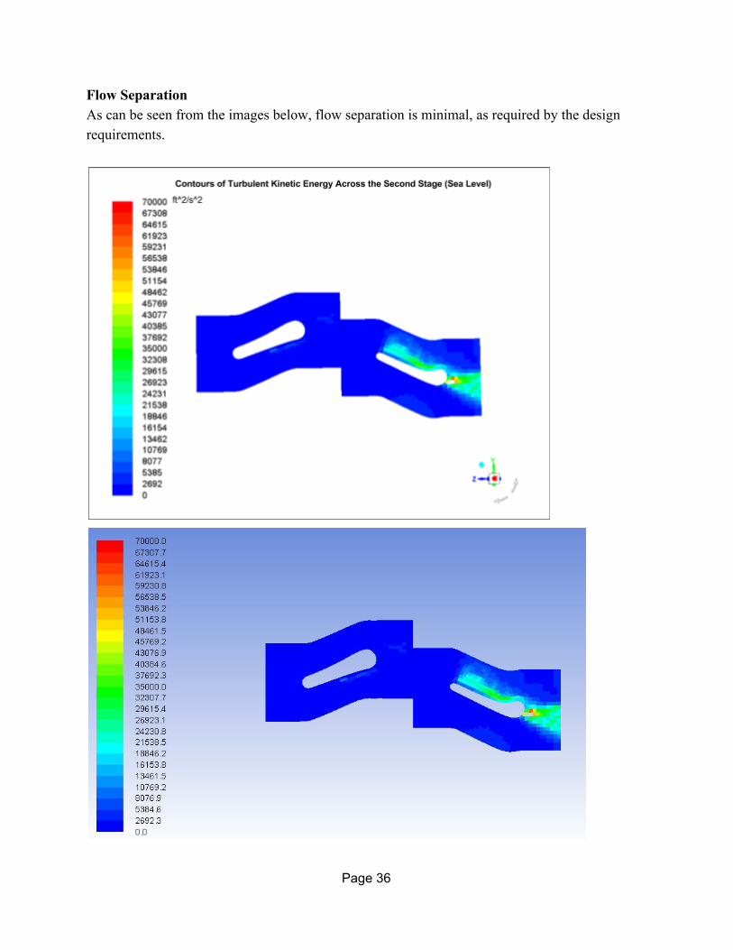
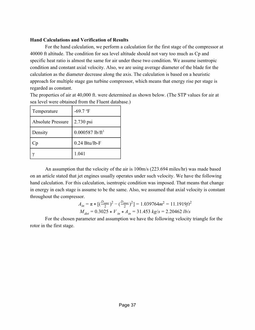
Flow Separation As can be seen from the images below, flow separation is minimal, as required by the design requirements.
Page 36
Hand Calculations and Verification of Results
For the hand calculation, we perform a calculation for the first stage of the compressor at 40000 ft altitude. The condition for sea level altitude should not vary too much as Cp and specific heat ratio is almost the same for air under these two condition. We assume isentropic condition and constant axial velocity. Also, we are using average diameter of the blade for the calculation as the diameter decrease along the axis. The calculation is based on a heuristic approach for multiple stage gas turbine compressor, which means that energy rise per stage is regarded as constant. The properties of air at 40,000 ft. were determined as shown below. (The STP values for air at sea level were obtained from the Fluent database.)
Temperature -69.7 oF
Absolute Pressure 2.730 psi
Density 0.000587 lb/ft3
Cp 0.24 Btu/lb-F
γ 1.041
An assumption that the velocity of the air is 100m/s (223.694 miles/hr) was made based
on an article stated that jet engines usually operates under such velocity. We have the following hand calculation. For this calculation, isentropic condition was imposed. That means that change in energy in each stage is assume to be the same. Also, we assumed that axial velocity is constant throughout the compressor.
( ) ) ] .039764m 1.1919f tAin = π * [ 2Douter 2 − ( 2
Dinner 2 = 1 2 = 1 2 .3025 1.453 kg/s .20462 lb/sM dot = 0 * V in * Ain = 3 = 2
For the chosen parameter and assumption we have the following velocity triangle for the rotor in the first stage.
Page 37
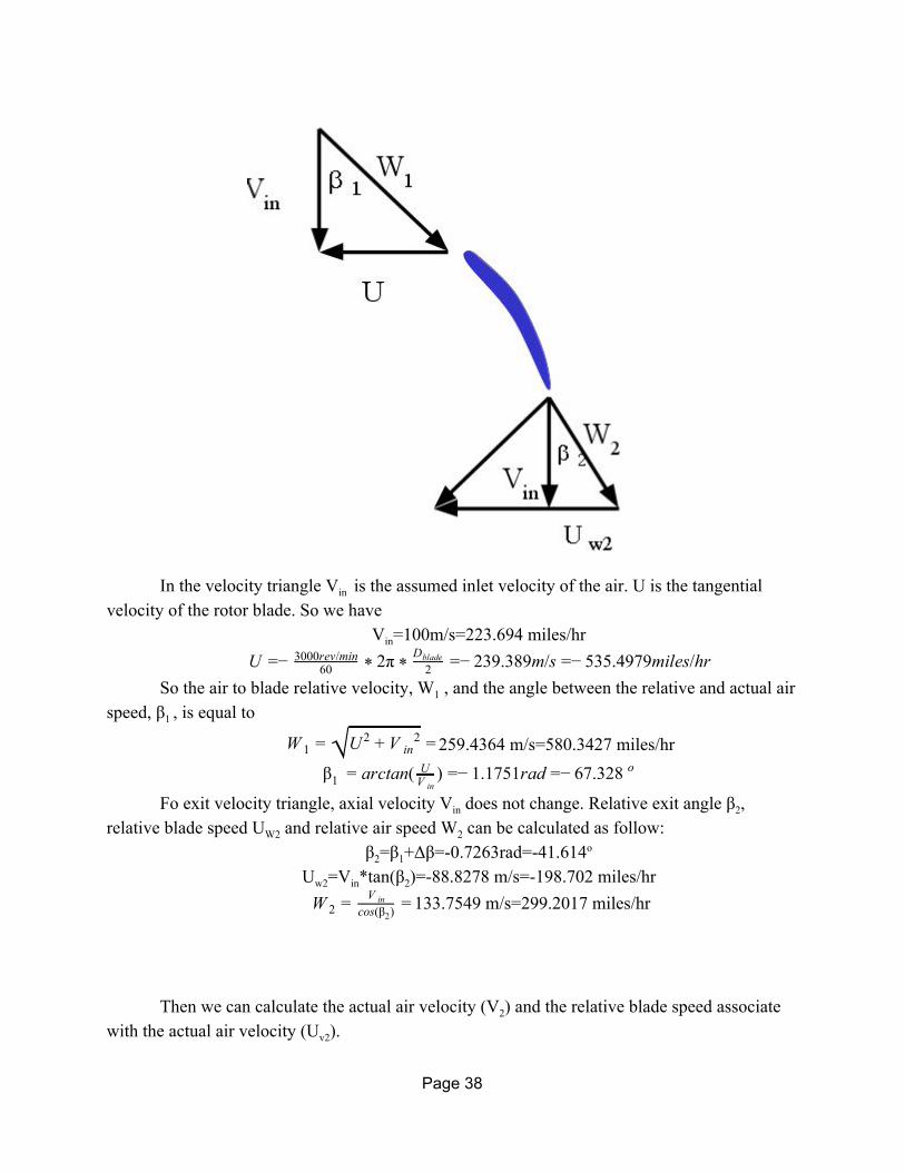
In the velocity triangle Vin is the assumed inlet velocity of the air. U is the tangential
velocity of the rotor blade. So we have Vin=100m/s=223.694 miles/hr
− π − 39.389m/s − 35.4979miles/hrU = 603000rev/min * 2 * 2
Dblade = 2 = 5 So the air to blade relative velocity, W1 , and the angle between the relative and actual air
speed, β1 , is equal to
259.4364 m/s=580.3427 miles/hr W 1 = √U 2 + V in2 =
rctan( ) − .1751rad − 7.328 β1 = a U
V in= 1 = 6 o
Fo exit velocity triangle, axial velocity Vin does not change. Relative exit angle β2, relative blade speed UW2 and relative air speed W2 can be calculated as follow:
β2=β1+Δβ=-0.7263rad=-41.614o Uw2=Vin*tan(β2)=-88.8278 m/s=-198.702 miles/hr
133.7549 m/s=299.2017 miles/hrW 2 = V incos(β )2
=
Then we can calculate the actual air velocity (V2) and the relative blade speed associate
with the actual air velocity (Uv2).
Page 38
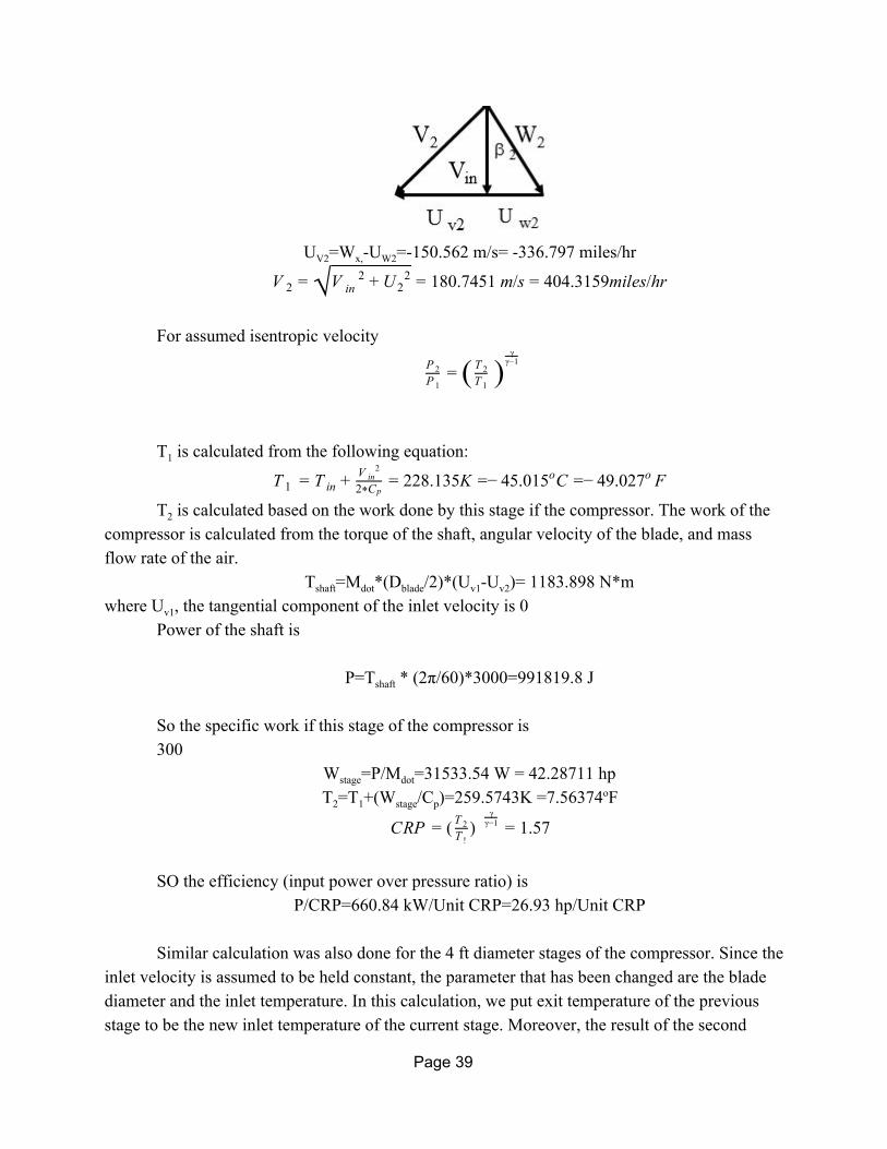
UV2=Wx,-UW2=-150.562 m/s= -336.797 miles/hr
80.7451 m/s 04.3159miles/hr V 2 = √V in 2 + U 2
2 = 1 = 4
For assumed isentropic velocity
P 1
P 2 = ( T 1
T 2 )
γγ−1
T1 is calculated from the following equation:
28.135K − 5.015 C − 9.027 FT 1 = T in + V in
2
2 C* p= 2 = 4 o = 4 o
T2 is calculated based on the work done by this stage if the compressor. The work of the compressor is calculated from the torque of the shaft, angular velocity of the blade, and mass flow rate of the air.
Tshaft=Mdot*(Dblade/2)*(Uv1-Uv2)= 1183.898 N*m where Uv1, the tangential component of the inlet velocity is 0
Power of the shaft is
P=Tshaft * (2π/60)*3000=991819.8 J
So the specific work if this stage of the compressor is 300
Wstage=P/Mdot=31533.54 W = 42.28711 hp T2=T1+(Wstage/Cp)=259.5743K =7.56374oF
RP ) .57C = ( T !
T 2 γ
γ−1 = 1
SO the efficiency (input power over pressure ratio) is
P/CRP=660.84 kW/Unit CRP=26.93 hp/Unit CRP Similar calculation was also done for the 4 ft diameter stages of the compressor. Since the
inlet velocity is assumed to be held constant, the parameter that has been changed are the blade diameter and the inlet temperature. In this calculation, we put exit temperature of the previous stage to be the new inlet temperature of the current stage. Moreover, the result of the second
Page 39
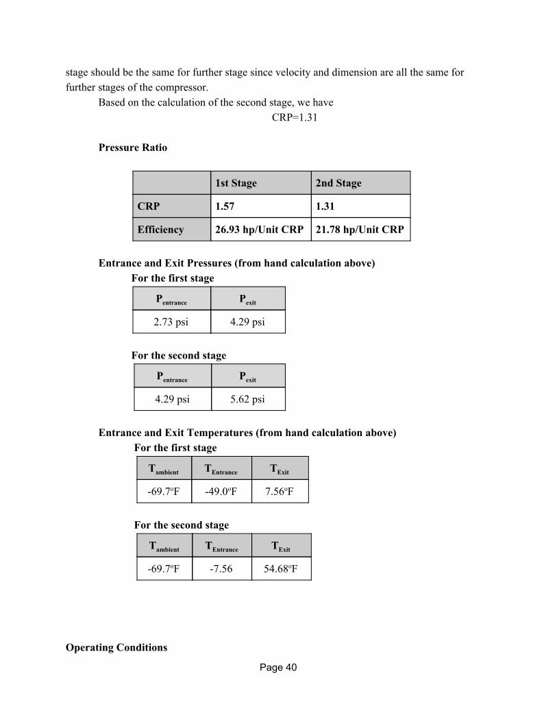
stage should be the same for further stage since velocity and dimension are all the same for further stages of the compressor.
Based on the calculation of the second stage, we have CRP=1.31
Pressure Ratio
1st Stage 2nd Stage
CRP 1.57 1.31
Efficiency 26.93 hp/Unit CRP 21.78 hp/Unit CRP
Entrance and Exit Pressures (from hand calculation above)
For the first stage
Pentrance Pexit
2.73 psi 4.29 psi
For the second stage
Pentrance Pexit
4.29 psi 5.62 psi
Entrance and Exit Temperatures (from hand calculation above)
For the first stage
Tambient TEntrance TExit
-69.7oF -49.0oF 7.56oF
For the second stage
Tambient TEntrance TExit
-69.7oF -7.56 54.68oF
Operating Conditions
Page 40
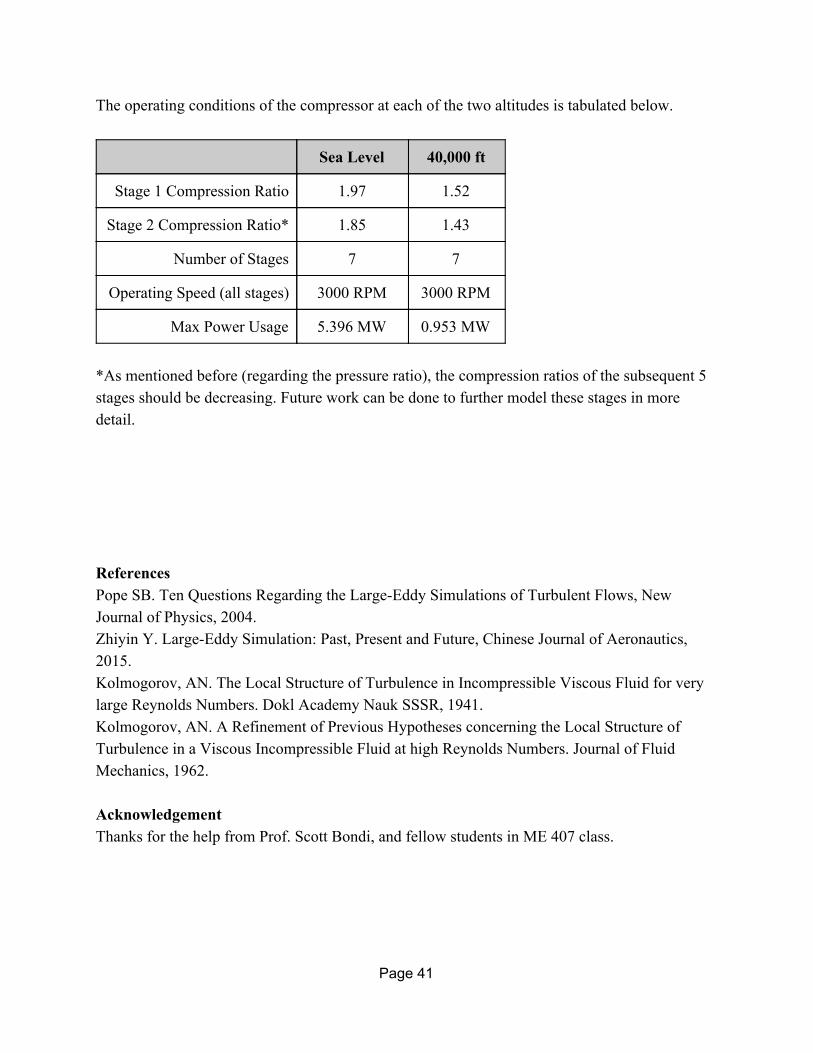
The operating conditions of the compressor at each of the two altitudes is tabulated below.
Sea Level 40,000 ft
Stage 1 Compression Ratio 1.97 1.52
Stage 2 Compression Ratio* 1.85 1.43
Number of Stages 7 7
Operating Speed (all stages) 3000 RPM 3000 RPM
Max Power Usage 5.396 MW 0.953 MW
*As mentioned before (regarding the pressure ratio), the compression ratios of the subsequent 5 stages should be decreasing. Future work can be done to further model these stages in more detail. References Pope SB. Ten Questions Regarding the Large-Eddy Simulations of Turbulent Flows, New Journal of Physics, 2004. Zhiyin Y. Large-Eddy Simulation: Past, Present and Future, Chinese Journal of Aeronautics, 2015. Kolmogorov, AN. The Local Structure of Turbulence in Incompressible Viscous Fluid for very large Reynolds Numbers. Dokl Academy Nauk SSSR, 1941. Kolmogorov, AN. A Refinement of Previous Hypotheses concerning the Local Structure of Turbulence in a Viscous Incompressible Fluid at high Reynolds Numbers. Journal of Fluid Mechanics, 1962. Acknowledgement Thanks for the help from Prof. Scott Bondi, and fellow students in ME 407 class.
Page 41