awwa water conservation measurement metrics dev... · water conservation measurement metrics ......
TRANSCRIPT

The American Water Works Association Water Conservation Division Subcommittee Report
January 2010
WATER CONSERVATION MEASUREMENT METRICS Guidance Report Ben Dziegielewski and Jack C. Kiefer
Copyright © 2009 American Water Works Association, Ben Dziegielewski, and Jack C. Kiefer. All Rights Reserved 2
WATER CONSERVATION MEASUREMENT METRICS
GUIDANCE REPORT
Prepared by:
Ben Dziegielewski, Ph.D. Southern Illinois University Carbondale
and
Jack C. Kiefer, Ph.D.
Hazen and Sawyer, P.C.
Submitted to:
The American Water Works Association Water Conservation Division Subcommittee:
Mary Ann Dickinson, AWE, Chair, David Bracciano, Tampa Bay Water
Al Dietemann, Seattle Public Utilities Peter Mayer, Aquacraft, Inc.
Marjie Risk, Lone Star Groundwater Conservation District Cheri Vogel, New Mexico Office of the State Engineer
Project funded by the AWWA Technical & Education Council
and sponsored by the Water Conservation Division
January 22, 2010

Copyright © 2009 American Water Works Association, Ben Dziegielewski, and Jack C. Kiefer. All Rights Reserved
ACKNOWLEDGEMENTS
The authors wish to acknowledge the guidance and contributions to this report which were provided by the Members of the American Water Works Association Water Conservation Division Subcommittee: Mary Ann Dickinson, Alliance for Water Efficiency, Chair David Bracciano, Tampa Bay Water Al Dietemann, Seattle Public Utilities Peter Mayer, Aquacraft, Inc. Marjie Risk, Lone Star Groundwater Conservation District Cheri Vogel, New Mexico Office of the State Engineer These individuals offered important insights on the issues of water use and conservation measurement and guided the development of iterative drafts of the project report. We are also grateful to the participating water utilities that provided data on water production and customer billing summaries, which were used for illustrative purposes in this report. We are especially grateful to the individuals who helped us assemble the relevant data: Al Dietemann, Seattle Public Utilities William E. Granger, Otay Water District George Kunkel, Philadelphia Water Department Adam Q. Miller, Phoenix Water Services Department Seung Park and Ramiro Vega, City of Tampa Water Department Fiona Sanchez, Irvine Ranch Water District Marian Wrage, City of Rio Rancho
We also extend a special thanks to Mr. George Kunkel, Assistant Chief of Water Conveyance Section in Philadelphia for helping us revise the water losses section of the report. The study team is grateful to Ms. Elise Harrington of AWWA for contract and process management and to AWWA’s Technical &Education Council for providing financial support for the project.

Copyright © 2009 American Water Works Association, Ben Dziegielewski, and Jack C. Kiefer. All Rights Reserved ii
TABLE OF CONTENTS Section Title Page 1 PURPOSE 12 METRICS VERSUS BENCHMARKS 12.1 Definition of a Metric 12.2 Definition of a Benchmark 22.3 Defining Efficiency 22.4 Terminology and Acronyms 33 DATA FOR CALCULATING METRICS 43.1 Production and Sales Data 43.2 Data on Scaling Variables 43.3 Special Studies 54 CASE STUDY UTILITIES 54.1 Characteristics of Study Sites 65 METRICS OF AGGREGATE USE 85.1 Per Capita Daily Production Metric 85.2 Alternatives to the PQc Metric 105.3 Inter-utility Comparisons of Aggregate Metrics 136 SECTOR-WIDE ANNUAL USE METRICS 146.1 Single-Family Residential Use 156.2 Multifamily Residential Use 156.3 Nonresidential Use 167 SEASONAL AND NONSEASONAL USE METRICS 177.1 Estimation of Seasonal/Nonseasonal and Outdoor/Indoor Use 177.2 Single-Family Indoor (Nonseasonal) Use Metrics 187.3 Single-Family Outdoor (Seasonal) Use Metrics 207.4 Multifamily Indoor Use Metrics 217.5 Multifamily Outdoor Use Metrics 227.6 Seasonal and Nonseasonal Nonresidential Metrics 228 NORMALIZING METRICS FOR COMPARABILITY 238.1 Single Utility Comparison 248.2 Cross-Utility Comparison 259 WATER CONSERVATION BENCHMARKS 259.1 Water Loss Metrics and Benchmarks 259.2 Indoor Conservation Indices 299.2.1 Single Family Indoor Use 309.2.2 Multifamily Indoor Use 319.3 Outdoor Conservation Indices 3210 SUMMARY RECOMMENDATIONS 3410.1 Applicability of Metrics 3410.2 Key Findings 3510.3 Recommendations 36 NOTATION 37 REFERENCES 38 APPENDIX A 39

Copyright © 2009 American Water Works Association, Ben Dziegielewski, and Jack C. Kiefer. All Rights Reserved iii
LIST OF TABLES Table 1 Water Utility Participants in the Study (2008 Data) 6Table 2 Growing Season (May-September) Climatic Data for Participating Utilities 7Table 3 Calculated Per Capita Production Metric (PQc ) for Participating Utilities 9Table 4 Calculated Production per Account (PQa) Metric for Participating Utilities 10Table 5 Weighting Ratios and Equivalent Accounts Based on 2008 Sales Data 12Table 6 Weighting Ratios Based on Meter Size for Philadelphia 12Table 7 Calculated Aggregate Metrics for Participating Utilities for 2008 13Table 8 Annual Single-Family Residential Use per Account 15Table 9 Annual Multifamily Residential Use per Account 16Table 10 Annual Nonresidential Use per Account (Gallons per Account per Day) 16Table 11 Monthly and Seasonal Single-Family Water Sales per Account in 2008 19Table 12 Single Family Indoor Water Use per Account 20Table 13 Single Family Outdoor Water Use per Account 21Table 14 Multifamily Indoor Water Use per Account 22Table 15 Multifamily Outdoor Water Use per Account 22Table 16 Nonseasonal Nonresidential (Indoor) Water Use per Account 23Table 17 Nonseasonal Nonresidential (Outdoor) Water Use per Account 23Table 18 System-Wide Metrics of Water Losses 26Table 19 IWA/AWWA Standard Water Balance Terms 27Table 20 Examples of Water Loss Metrics for Philadelphia 28Table 21 Comparison of Nonrevenue Water Metric 28Table 22 Example of Calculations for Toilet End Use 30Table 23 Examples of Average and Efficient Levels of Indoor Residential End Uses 31Table 24 Examples of Average and Efficient Levels of Indoor Residential End Uses in
Multifamily Sector 32Table 25 Metrics of Water Use and Conservation 34 APPENDIX TABLES
Table O1 Annual Production, Sales and Billed Accounts Data for Otay Water District,
California 40Table O2 Calculated Metrics Using the Number of Accounts and Population Served as
Normalizing Variables for Otay Water District, California 41Table O3 Metrics Based on Socioeconomic Data for Otay, California 42Table O4 Monthly and Seasonal Single-Family Residential Usage Rates in Otay, California. 42Table O5 Monthly and Seasonal Multifamily Residential Usage Rates in Otay, California. 43Table O6 Monthly and Seasonal Nonresidential (Commercial/Public/Construction)
Usage Rates in Otay, California 43Table O7 System-wide Production, Consumption and Losses in Otay WD 44Table I1 Reported Production and Sales Data for Irvine Ranch Water District, California 45Table I2 Customer Classification and Number of Accounts in Irvine Ranch, California 46Table I3 Summary of Billed Accounts in Irvine Ranch Water District, California 47Table I4 Calculated Metrics Using the Number of Accounts as Normalizing Variable 47Table I5 Monthly and Seasonal Single-Family Residential Usage Rates in Irvine Ranch,
California. 48Table I6 Monthly and Seasonal Multifamily Residential Usage Rates in Irvine Ranch,
California. 48Table I7 Monthly and Seasonal Nonresidential Usage Rates in Irvine Ranch, California. 49

Copyright © 2009 American Water Works Association, Ben Dziegielewski, and Jack C. Kiefer. All Rights Reserved iv
Table P1 Number of Accounts by Customer Category in Phoenix Water Services Department, Arizona 50
Table P2 Average Water Use per Account by Customer Category in Phoenix Water Services Department, Arizona 51
Table P3 Monthly and Seasonal Single-Family Usage Rates per Account per Day in Phoenix, Arizona 52
Table P4 Monthly and Seasonal Apartments Usage Rates per Account per Day in Phoenix, Arizona 52
Table P5 Monthly and Seasonal General Commercial Usage Rates per Account per Day in Phoenix, Arizona 53
Table R1 2008 Production, Sales and Number of Accounts for Rio Rancho, New Mexico 53Table R2 2008 Monthly and Seasonal Water Use in Rio Rancho 54Table S1 Reported 2008 Production and Sales Data for Seattle, Washington 55Table S2 Monthly Water Use in Single-Family Sector in Seattle in 2008. 56Table S3 Monthly Water Use in Multifamily Sector in Seattle in 2008. 56Table S4 Monthly Water Use in Nonresidential Sector in Seattle in 2008 57Table S5 Historical Water Use in Single-Family and Multifamily Sectors in Seattle 57Table L1 System-wide Production, Consumption and Losses in Philadelphia in 2008 58Table L2 Historical Production, Consumption and Water Losses in Philadelphia 59Table T1 Annual Production, Sales and Billed Accounts Data for Tampa Water Department,
Florida 60Table T2 Calculated Metrics Using the Number of Accounts and Population Served as
Normalizing Variables in Tampa 61Table T3 Monthly and Seasonal Single-Family Residential Usage Rates in Tampa, Florida. 61Table T4 Monthly and Seasonal Multifamily Residential Usage Rates in Tampa, Florida. 62Table T5 Monthly and Seasonal Nonresidential Usage Rates in Tampa, Florida. 62 LIST OF FIGURES Figure 1 Relationship between Per Capita Production and Evapotranspiration minus Effective
Rainfall during Growing Season 10Figure 2 Estimated Single-Family Outdoor Use vs. Theoretical Irrigation Demand during
Growing Season 21

Copyright © 2009 American Water Works Association, Ben Dziegielewski, and Jack C. Kiefer. All Rights Reserved 1
WATER CONSERVATION MEASUREMENT METRICS: GUIDANCE REPORT
By Ben Dziegielewski and Jack C. Kiefer January 22, 2010
1. PURPOSE
Public water supply utilities need quantitative metrics and benchmarks in order to assess their success in achieving water efficiency goals. Such metrics and benchmarks have to be explicitly and appropriately defined. They also have to be characterized in terms of their value in making comparisons between different periods of time for a single utility or across different utilities.
The purpose of this guidance report is to identify and characterize a set of water use and conservation metrics for public water supply utilities. These metrics could be used as measurement tools to evaluate the effects of water efficiency programs over time in a single utility. Some metrics can also be used to compare water use and conservation effects across different utilities. This report provides guidance on standardized methods of calculating specific metrics and describes their advantages and limitations. The calculation and use of metrics are illustrated using data from seven water utilities in the U.S. that agreed to participate in the project.
2. METRICS VERSUS BENCHMARKS
Before providing guidance on specific metrics it is important to clarify the terminology and potential uses of metrics and benchmarks. While the terms “metric” and “benchmark” are sometimes used interchangeably, for the purpose of this report stricter definitions are adopted in the context of evaluating the use of water. These are described below.
2.1 Definition of a Metric
A metric is a unit of measure (or a parameter being measured) that can be used to assess the rate of water use during a given period of time and at a given level of data aggregation (e.g., system-wide, sector-wide, customer level, or end-use level). Another term for a metric is performance indicator.
Basically, a metric is a formula. In the context of measuring water use, there are very many possible metrics that can be formulated. Some examples of water usage metrics include: total water use per capita per day; residential indoor water use per dwelling unit per day; or average volume of water being used for flushing toilets.
A mathematical formula can be applied to water use and related data from a utility for a defined time period to obtain a numerical value of any given metric. This value can be compared to a pre-defined benchmark value to assess a relative level of performance. It is important to remember that the calculated value of a metric of water usage is not a benchmark value.
A number of different metrics for measuring water usage rates can be devised. However, the ability to develop the corresponding benchmark values depends on the level of data aggregation and other considerations.

Copyright © 2009 American Water Works Association, Ben Dziegielewski, and Jack C. Kiefer. All Rights Reserved 2
2.2 Definition of a Benchmark
A benchmark is a particular (numerical) value of a metric that denotes a specific level of performance, such as a water efficiency target. Sometimes a distinction is made between a benchmark (which indicates a current state of achievement) and a target which indicates a state of achievement expected at some time in the future.
Basically, benchmarks or targets are numerical values of the metric to which the calculated metric values are intended to be compared. Metrics and benchmarks can be defined in either absolute or relative terms. For example, some broadly defined benchmarks may reflect conservation goals of water utility, which are often expressed in relative terms, such as a 15 percent reduction of average annual per capita water use in 10 years.
Examples of specific absolute-value benchmarks include: Energy Policy Act of 1992 requirement that all residential toilets had to flush using no more than 1.6 gallons per flush; or Energy Star residential clothes washer standard water factor WF ≤ 8.0 gallons per cycle per cubic foot. Here, the values of 1.6 gallons and 8.0 gallons are benchmarks, which are expressed in absolute terms (i.e., quantity of water being used). Examples of metrics and benchmarks for nonresidential users can be found in Dziegielewski at al. (2000).
Relative-value metrics are ratios without units. For ratio metrics, a value of 1 often represents a target value. An example of the ratio benchmark is the Infrastructure Leakage Index (ILI) developed by the American Water Works Association and the International Water Association (IWA). It is calculated as a ratio of the current annual real losses of water in the distribution system to the unavoidable annual real losses. For most utilities the calculated values of ILI will be greater than 1. Here, the ILI = 1.0 is the benchmark value (or target) which implies that all avoidable losses of water are eliminated. Similar ratio benchmarks can be defined for various end uses of water, where the observed usage rate is divided by an achievable efficient rate of use.
Development of benchmark values for aggregate-level metrics (such as system-wide or sector-wide measures) presents a special challenge for evaluating water efficiency, because the aggregate metrics capture “other-than-efficiency” effects on the calculated unit quantity of water usage. This is a critical point because aggregate-level metrics tend to be interpreted as an indicator of efficiency-in-use, when in reality the calculated values reflect the influence of various other determinants of water use, which are unrelated to efficiency-in-use.
2.3 Defining Efficiency
Improvements in the efficiency of water use are usually undertaken by water providers and water users. A commonly held expectation is that such improvements can free up significant quantities of water by meeting the existing needs of individual users and various purposes of use with less water. Water use metrics and benchmarks are inextricably linked to the concepts of “water conservation” and “water-use efficiency.” Therefore, it is also helpful to define these concepts in the context of evaluating water use.
The term, efficiency, derives from engineering practice where it is typically used to describe technical efficiency, or the ratio of output to input. The criterion of technical efficiency is useful in comparing various products and processes. For example, one showerhead would be considered more efficient than another if it could accomplish the same purpose (i.e., of showering) by using less water

Copyright © 2009 American Water Works Association, Ben Dziegielewski, and Jack C. Kiefer. All Rights Reserved 3
or other inputs (e.g., lower water pressure). The water efficiency gains of low flushing volume toilets over traditional toilets can be substantial without diminishing the completion of the original purpose for which water is used. However, the technical efficiency concept is not useful in making decisions of investing money (or resources) in water conservation unless the inputs and outputs are measured in value terms. This expression of efficiency is referred to as economic efficiency.
Water conservation can be defined as a reduction in water use or water losses. Baumann, Boland and Sims (1984) developed a practical definition of long-term water conservation as “…any beneficial reduction in water use or in water losses.” By adding the term “beneficial” the authors proposed a requirement (consistent with the concept of economic efficiency) that the reduction in water use or losses should result in a net increase in social welfare where the resources used have a lesser value than those saved. In other words, the beneficial effects of the reduction in water use (or loss) must be considered greater than the adverse effects associated with the commitment of other resources to the conservation effort. This definition provided important guidance (through benefit-cost analysis) for long-term conservation; however, it could not be easily applied to short-term conservation measures which are usually aimed at curtailing water demand during a drought.1
2.4 Terminology and Acronyms
The purpose of this paper is to define “water conservation metrics” and benchmarks. A necessary intermediate step is to define “water use metrics” so that a reduction in water use can be quantified. However, the term water use has multiple meanings depending on whether it is used in hydrologic, engineering or regulatory contexts. The term water use could mean total water withdrawals from different supply sources, water withdrawn or diverted and put to beneficial use, finished drinking water produced, water sold to customers through metered connections, and many other meanings. In this document the phrase “water use” is used as a generic term with the meaning defined by the context.
Water use metrics (designated by the acronym - UM) can be expressed as “usage ratios” or “usage rates”. The “ratio” metric designates the quotient obtained by dividing the volume of water sold over a specified period of time (day, month, season or year) by a scaling factor (e.g., number of accounts, population served or number of employees). Additional letters, superscripts and subscripts can be added to the UM acronym to designate user sector and the scaling variable being used. For example, the annual average usage rate per customer account per day in single family sector can be designated as AUMa
SF, where “A” stands for annual (i.e., average daily), “a” for accounts and “SF” for single family.
For water production and deliveries, the term “production quotient,” or PQ is proposed. It represents the total volume of water produced divided by a scaling factor such as number of connections or population served. For example, the annual average rate of water production per service account would be designated as APQa.
The term “conservation index” or CI is proposed as the naming convention for denoting conservation metrics. An example could be ICISF for designating an indoor conservation index for the single-family sector and OCISF for designating an outdoor (seasonal) conservation index.
1 Temporary restrictions on water use are usually undertaken in order to prevent adverse impacts of severe shortages in the future if the drought continues and their outcomes cannot be easily analyzed through benefit-cost analysis.

Copyright © 2009 American Water Works Association, Ben Dziegielewski, and Jack C. Kiefer. All Rights Reserved 4
3 DATA FOR CALCULATING METRICS
3.1 Production and Sales Data
The most practicable water usage metrics are those that can be calculated using secondary (i.e., existing) and routinely collected data. Generally, there are two types of existing water measurement records that are routinely collected and maintained by public water supply utilities. These include:
(1) water production records (i.e., amounts of water pumped into the distribution system), and
(2) meter reading and billing records (i.e., amounts of water used by each customer during each billing period and related information).
Water production records show the amount of water delivered to the distribution system and are typically generated daily or hourly. Water production data are almost always available because they represent an essential operating parameter for treatment, distribution and water accounting. Production metering provides measured quantities of water being pumped from treatment plants and other sources to the distribution system. Production meters are usually inserted just before water exits the treatment facility and is delivered to the distribution system. The accuracy of production data is generally good and depends on the accuracy of production meters.
Meter reading and billing records represent the individual customer account data that are maintained by retail water supply agencies. An individual billing record commonly includes: (1) name and address of account holder, (2) type of account (e.g., single-family, commercial, industrial, institutional, irrigation or other), (3) meter size, (4) meter readings and the dates of meter readings, (5) water use between meter readings, and (6) billing information (charges incurred, dates paid, etc.). The customer billing system is usually computerized, and, depending on the database design, individual customer accounts can be sorted and queried by customer type, geographical area, and other characteristics.
Billing records can usually be summarized by aggregating metered consumption and number of billed accounts by the billing cycle (i.e., monthly, bimonthly, quarterly, semiannually, or annually) and by customer type. In essence, water billing data show how much water is being sold to different types of customers, but do not show for which specific purposes the water is being used.
3.2 Data on Scaling Variables
Summaries of billing system data generally contain information on the volume of water being sold and the number of billed accounts. Therefore, other than for the number of billed accounts, data on alternative scaling variables—that is, variables that can be used to standardize per unit rates of water use— have to be obtained from other sources. Some common scaling variables include: population served, number of housing units, number of employees, acreage of irrigated areas, square footage of nonresidential buildings, and other measures of size for specific sectors of water users.

Copyright © 2009 American Water Works Association, Ben Dziegielewski, and Jack C. Kiefer. All Rights Reserved 5
Perhaps the most common scaling variable in public water supply utilities is “population served.” In theory, it represents the number of people who are served (through metered connections) by the water utility. However, even this basic scaling variable is very challenging to define (in operational terms) and measure precisely. In the water utility service area, several types of populations can be distinguished. These include such designations as year-round (or resident) population, population in households, population in group quarters, commuter population, seasonal population and others.
Another issue with “population served” is the challenge in measuring these different populations. Relatively accurate estimates of resident population are made every ten years during the decennial census. Estimates of resident population during non-census years are obtained by alternative methods and are less accurate. Even during the census years, population counts available for census tracts and city blocks cannot be matched perfectly with the boundaries of areas served by water utility.
The appropriate measurement of population served is most challenging when it is used in water allocation (through water use permits) or for other regulatory purposes.2 For the purpose of developing water use and conservation metrics, the only scaling variable that is readily available to water utilities and more accurate than population served (or other measures of size from external sources) is the number of active or billed accounts.
3.3 Special Studies
Other (more disaggregated) data for calculating metrics of water use can be obtained through special measurements (e.g., data logging on customer meters, or installation and reading of special meters), as well as through the use of customer surveys to collect information on important variables that influence water use. Some large U.S. utilities conduct extensive “baseline” studies to collect information on a variety of customer characteristics (such as number of residents or employees, square footage of buildings or size of landscaped areas), as well as prevailing water-using behaviors (e.g., frequency of lawn watering, washing machine use, or the presence of water using features and appliances).
Because these data are not routinely collected by water utilities, the use of metrics that require special baseline data has to be limited to those that support the specific objectives of any particular investigation. Thus, this study employs only data that are routinely collected by water utilities, focusing on summary level production and billing data.
4 CASE STUDY UTILITIES
Ten U.S. water utilities were asked to participate in this study. Seven utilities agreed to participate. The utilities were asked to provide their summary production and billing records for the five most recent data years. Table 1 lists the seven utilities together with the water production, number of customer accounts and estimated population served data for 2008.
2 Examples of complex methodologies for calculating population served are those developed by the Southwest Florida Water Management District (Gonzales and Yingling, 2008) and New Mexico Office of State Engineer (2009).

Copyright © 2009 American Water Works Association, Ben Dziegielewski, and Jack C. Kiefer. All Rights Reserved 6
Table 1. Water Utility Participants in the Study (2008 Data)
Water Utility Water
Production (MGD)
Number of Customer Accounts
Estimated Population
Served Otay Water District, California 37.1 48,227 196,416 Irvine Ranch Water District, California 88.2 96,019 330,000 Phoenix Water Services Department, Arizona 272.8 403,412 1,566,190 City of Rio Rancho, New Mexico 11.7 29,787 80,000 Seattle Public Utilities, Washington 125.5 186,849 649,286 Philadelphia Water Department, Pennsylvania 250.7 486,664 1,660,500 Tampa Water Department, Florida 76.0 125,260 657,313
Notes: MGD = million gallons per day. The combined retail and wholesale population served in Seattle is 1,312,920.
4.1 Characteristics of Study Sites
The seven study sites differ in size and in prevailing climate and weather patterns. Five of the cities represent arid or semi-arid climates. The remaining two (Tampa and Philadelphia) have humid climates. The following are brief descriptions of each case study site:
• The Otay Water District provides water service to customers within 125.5 square miles of southeastern San Diego County in California which includes the communities of Spring Valley, La Presa, Rancho San Diego, Jamul, eastern Chula Vista, and eastern Otay Mesa. The service area is semi-arid with an average annual precipitation of about 11 inches.
• The Irvine Ranch Water District (IWRD) is located in the south-central Orange County in California and serves the city of Irvine and portions of Costa Mesa, Lake Forest, Newport Beach, Orange and Tustin. It provides potable water as well as tertiary-treated recycled water for landscape irrigation, agriculture and industrial and commercial users. The 179 square mile service area extends from the Pacific Coast and rises to the elevation of 3,200 feet at the foothills of Santa Ana Mountains. The region is semi-arid with an average annual precipitation of about 14 inches.
• The City of Phoenix Water Services Department provides water supply to about 1,566,000 residents within its 540-square mile service area in central Arizona. The city is located in the Salt River Valley, with a desert-type climate with low annual rainfall and low relative humidity, mild winters, and high daytime temperatures throughout the summer months. The average annual precipitation is about 8 inches.
• The City of Rio Rancho in New Mexico is located north of Albuquerque and it borders the Santa Ana Indian Reservation to the north, and the cities of Bernalillo and Corrales to the east. The city has a total area of 73.4 square miles and serves approximately 80,000 people. The climate is arid with warm summers and cold winters, and an average annual precipitation of about 9 inches.
• Seattle Public Utilities (SPU) Water Utility supplies potable water to the City of Seattle and to 21 wholesale customers (with 121 wholesale connections) in King County, Washington (in total, the population served is more than 1.3 million). The City of Seattle service area extends for 143 square miles and includes a population of about 650,000. The city has a mild oceanic climate with wet winters and dry summers with total annual precipitation of 37 inches.

Copyright © 2009 American Water Works Association, Ben Dziegielewski, and Jack C. Kiefer. All Rights Reserved 7
• The Philadelphia Water Department provides water to a 130 square mile service area in the Greater Philadelphia region of Pennsylvania with a population of about 1.66 million. The city has a humid subtropical climate with hot and humid summers and cold winters, although it is at the northern periphery of this Köppen climate zone. Precipitation is fairly evenly distributed throughout the year; with an average annual precipitation of 42 inches.
• The Tampa Water Department delivers drinking water to a service population of approximately 657,000 people in the Tampa Bay area in Florida. The city has a year-round semitropical climate with a remarkable summer thunderstorm season. From June through September, on an average of three out of four days, late afternoon thundershowers occur making Tampa one of the stormiest cities in the United States. Average annual precipitation varies from about 45 inches near Tampa Bay to over 50 inches in the northeast side of the service area.
Table 2 compares the climatic differences among the seven participating utilities. It shows the normal (1971-2000 average) and actual 2008 values of precipitation, maximum temperature and reference evapotranspiration during a defined 5-month growing season (i.e., May to September).3 The reference evapotranspiration (ETo) values were obtained from published sources for individual states with the exception of Philadelphia where ETo was estimated using the Thornthwaite method based on mean monthly temperature (Thornthwaite and Mather, 1955).
Table 2. Growing Season (May-September) Climatic Data for Participating Utilities
Precipitation (inches)
Max. Temperature(deg. F)
Evapotranspiration (inches) Water Utility
Normal 2008 Normal 2008 Normal 2008 Otay 0.6 0.3 74.4 73.3 32.7 28.5 Irvine Ranch 0.8 0.4 80.8 83.6 28.1 28.2 Phoenix 2.9 5.7 99.6 101.6 45.5 43.0 Rio Rancho 5.3 2.1 86.7 88.4 24.2 30.2 Seattle 6.7 6.7 71.0 70.0 18.0 12.9 Philadelphia 19.3 17.6 79.8 81.4 24.1 24.6 Tampa 29.0 25.2 88.8 89.3 25.8 24.5
Source: Annual Climatological Summary, NOAA. The stations used were:` San Diego Lindberg Field and Chula Vista for Otay; Irvine Ranch for IRWD; Phoenix Sky Harbor for Phoenix; Rio Rancho #1 for Rio Rancho; Seattle Tacoma Airport for Seattle; Philadelphia Airport for Philadelphia; and Tampa Airport for Tampa. Reference evaporation obtained from public sources in individual states.
The data indicate that the Otay and Irvine Ranch water service areas receive minimal rainfall during the growing season but tend to have mild temperatures. Phoenix and Rio Rancho receive small amounts of rainfall but experience very high temperatures. Seattle receives about seven inches of rainfall during the identified growing season and has the lowest maximum temperatures among all seven sites. Philadelphia and Tampa have substantially higher rainfall during growing season than the five western sites but in both locations the reference evapotranspiration is close to seasonal precipitation. It is apparent that each site has a unique climate. Only Otay and Irvine Ranch are comparable in terms of all three climatic variables during the growing season. 3 A customary five month growing season encompasses most areas of the U.S., although a longer season is possible in warmer climate zones.

Copyright © 2009 American Water Works Association, Ben Dziegielewski, and Jack C. Kiefer. All Rights Reserved 8
The data obtained from the participating utilities were used to calculate a number of possible water use metrics, including a subset of metrics for comparing water usage and the associated water conservation effects over time. These metrics are discussed and illustrated with the case study data below.
5 METRICS OF AGGREGATE USE
Several different metrics of aggregated water use (system-wide) can be defined. All three characteristics portrayed in Table 1 above (i.e., average daily production, number of customer accounts, and population served) can be used to represent the size of the water system and its service area. However, these measures of system size do not convey information on the intensity (or average rates) of water use. The average rates of use can be obtained by dividing average daily production or total customer sales by a scaling variable. As mentioned before, the most commonly used scaling variable is population served. A popular metric of aggregate use is known as “per capita use” in gallons per capita per day. This metric is obtained by dividing average daily production (in gallons) by total population served. The appropriate use and limitations of this metric and the availability of alternative aggregate metrics are discussed below.
5.1 Per Capita Daily Production Metric When calculating the per capita daily production (PQc) metric (where subscript c indicates per capita), the reported annual volumes of water produced should be matched with the population served in the retail service area. This requires that all wholesale water deliveries outside of the retail service area are metered and deducted from the production volume.4 Also, any water imported into the distribution system should be added to production records. Total population served is usually defined as total year-round resident population of the retail service area (urban planners sometimes define resident population as the number of people occupying space in the community on a 24 hour per day, seven-day-per-week, 52 weeks per year basis). Different water utilities use different definitions of population served and, regardless of the definition, in most cases the reported population served estimates represents best guesses of the actual but unknown number. Therefore, the annual per capita per day production (PQc) metric that is calculated by dividing annual water production by population served is usually inaccurate due to “definitional noise” in both the numerator and denominator of the metric. Table 3 illustrates the values of the PQc metric that were calculated using data from the seven case study utilities. The values of the metric were obtained by dividing the average daily production numbers by population served. The values in Table 3 show that per capita production rates change from year to year and differ greatly across the seven utilities. The last column and the last row show the average absolute deviation in the respective row and column data from the mean in each row or column. The average deviations across the utilities are generally six times greater than average deviations of annual data for each utility. Over relatively short time intervals, the year to year changes in a 4 Alternately, if the population served by wholesale customers is known, the PQ value can be calculated by dividing total production by the sum of retail and wholesale population served.

Copyright © 2009 American Water Works Association, Ben Dziegielewski, and Jack C. Kiefer. All Rights Reserved 9
single utility are caused primarily by changes in weather conditions. The differences across utilities are caused by two main factors: climate and the composition of water users. Figure 1 shows a plot of annual per capita values for 2008 versus the difference between reference evapotranspiration and effective precipitation during the 5-month growing season (only the 2008 data were available for all seven utilities). For six utilities the per capita values are more or less aligned with the theoretical irrigation water requirement during the growing season. The value for Irvine Ranch lies farther away from the regression line. Water production in Irvine Ranch district includes about 8 mgd of water delivered to agricultural customers and 2.6 mgd in wholesale deliveries.5 If these two quantities are subtracted from 2008 production, the per capita production would be 214 gpcd and the data point would be moved closer to the regression line.
Table 3. Calculated Per Capita Production Metric (PQc ) for Participating Utilities
Utility/Year 2002 2003 2004 2005 2006 2007 2008 Average Deviation
Otay 227 206 212 207 209 203 189 7.2 Irvine Ranch -- -- -- 252 279 268 267 7.3 Phoenix 228 211 207 197 198 196 174 11.8 Rio Rancho -- -- -- -- -- -- 146 -- Seattle 109 111 112 100 102 97 95 6.0 Philadelphia 160 166 162 157 153 155 151 4.2 Tampa -- -- 130 112 117 124 116 5.8 Avg. deviation 46.5 35.0 35.9 47.8 52.3 48.5 40.7 44.7
GPCD = gallons per capita per day, -- = data not available. Seattle numbers are based on the sum of both retail and wholesale population.
The data points for Rio Rancho and Phoenix lie below the regression line. In the case of Rio Rancho, the seemingly outlying per capita production value may be partly related to a possibly imprecise estimate of population served. The U.S. Census estimate of the 2007 population for the City of Rio Rancho is 75,978 while the number used in Table 1 (obtained from Rio Rancho’s website) is 80,000. Using this population, the per capita production would be 154 gpcd vs. the value of 146 shown on the graph. In Phoenix, the low 2008 value of 174 gpcd could not be explained by any possible imprecision in population or production.
According to the regression equation on Figure 1, per capita production increases by about 3.0 gpcd for each inch of irrigation requirement during growing season. The regression equation displayed on Figure 1 indicates that at zero requirement (when effective rainfall is equal to evapotranspiration) during the growing season the expected value of per capita production would be about 96.2 gallons per capita per day (gpcd). However, the 96.2 gpcd number has no practical value for deriving benchmark usage rates because of the differences in base climate. For example, it is unlikely that Phoenix would experience 96.2 gpcd during a growing season if precipitation was adequate for maintaining the urban landscapes. In essence, each locale or region should have its own regression line that best relates water use with local weather conditions.
5 It is important to note that while removing wholesale water from total production makes intuitive sense, removing agricultural deliveries would affect the difference in the composition of demand which tends to be unique in each utility.

Copyright © 2009 American Water Works Association, Ben Dziegielewski, and Jack C. Kiefer. All Rights Reserved 10
Figure 1. Relationship between Per Capita Production and Evapotranspiration minus Effective Rainfall
during Growing Season
5.2 Alternatives to the PQc Metric
Because population served is difficult to measure (even if it is precisely defined), a more accurate measure of system size is needed. One measure of system size that is universally available is the number of water service connections. This measure can be defined precisely by making distinctions between specific characteristics of the various types of connections.
For example, a distinction can be made between retail and wholesale connections, metered and unmetered connections and connections with different meter sizes. Alternative definitions include active and inactive customer accounts, customer accounts with non-zero consumption or number of billed accounts. Table 4 compares the average water use per account (i.e., the PQa metric where subscript a stands for accounts) in the seven utilities. The advantage of this metric is that the data on the number of connections (or accounts) are available on an annual basis. The number of billed accounts is also available for each billing period (i.e., monthly, bimonthly or quarterly). Billed accounts would include all accounts receiving a bill including connections with no metered use – only fixed charges.
Table 4. Calculated Production per Account (PQa) Metric for Participating Utilities
Utility/Year 2002 2003 2004 2005 2006 2007 2008 Average Deviation
Otay 832 773 802 781 794 801 769 16.1Irvine Ranch -- -- 886 868 943 908 892 20.9Phoenix 865 799 775 743 753 738 659 44.0Rio Rancho -- -- -- -- -- -- 393 --Seattle -- -- -- -- -- -- 670 --Philadelphia 554 570 557 552 539 543 515 12.7Tampa -- -- 643 596 603 647 607 20.6Avg. deviation 130.9 96.0 106.1 107.2 124.2 106.0 118.9 119.7
PQa = production per account per day in gallons, -- = data not available

Copyright © 2009 American Water Works Association, Ben Dziegielewski, and Jack C. Kiefer. All Rights Reserved 11
As with the per capita production, the PQa metric can be used for comparing year-to-year changes in production per account in a single utility. The PQa metric is still inappropriate for inter-utility comparisons. The calculated values of the PQa metric in Table 4 for 2008 ranged from 393 gpad in Rio Rancho to 892 in Irvine Ranch. However, the 2008 values of PQa include wholesale deliveries of water in Otay, Irvine Ranch, Tampa and Seattle, while for Phoenix and Rio Rancho they do not. Therefore, the PQa metric can be standardized by narrowing down its definition to include only “water deliveries to the retail area” which would exclude the part of water production sold wholesale.6 For example, if wholesale deliveries in Seattle are excluded, the value of the 2008 PQa metric would be 302 gpad. The PQa metric can also be refined further by using total metered sales as the numerator. This modification will remove the effect of non-revenue water, which is usually addressed by separate metrics. Furthermore, wholesale deliveries and agricultural sales can be removed from total metered sales.
Another improvement to the PQa would be to convert the total number of connections or accounts (which represent different types of customers or connection sizes) into the number of “equivalent connections” or “equivalent accounts”, with reference to single-family accounts. The weights for converting non-single-family accounts into equivalent single-family accounts can be based on average annual consumption by customer type or by meter size (in utilities without customer type designation). The main reason for creating a number of equivalent accounts for each utility is to develop a scaling variable which is similar to population served. Table 5 compares possible weights for calculating the number of equivalent accounts in the six study areas. The city of Philadelphia does not use customer categories and the only feasible weights are those based on average consumption by meter size category.
The weighing ratios in Table 5 illustrate the differences in the composition of demands at the sectoral level. For example, it is important to understand why an industrial customer is on average equal to 106.5 single-family customers in Phoenix, but equal only to 19.6 single-family customers in Irvine Ranch. Also, it is worth determining why a multifamily customer in Tampa is equivalent to 28.6 single-family customers and equates only to 3.1 single-family customers in Rio Rancho. It was determined that in Rio Rancho the multifamily sector includes only tri- and four-plexes. Apartments with five and more units are classified as commercial. Apparently, in Tampa all residential customers other than single-family are included in the multifamily sector. These examples of customer class definitions indicate another source of definitional noise introduced by unique customer classifications schemes.
Table 6 shows the calculated weights based on the 2008 sales data for accounts with different meter sizes in Philadelphia. The single-family sector is assumed to be represented by the meter size of 5/8 of an inch.
6 However, the removal of the wholesale deliveries from the production data is not straightforward. Total production is metered accurately on the daily basis while the wholesale deliveries may be reported on monthly basis. Also, line losses between the production meter and the wholesale connection cannot be easily measured.

Copyright © 2009 American Water Works Association, Ben Dziegielewski, and Jack C. Kiefer. All Rights Reserved 12
Table 5. Weighting Ratios and Equivalent Accounts Based on 2008 Sales Data
User Category Otay Irvine Ranch Phoenix Rio
Rancho Seattle Tampa
Single-family 1.0 1.0 1.0 1.0 1.0 1.0Multifamily 8.4 5.9 6.8 3.1 4.4 28.6Commercial 3.9 11.9 4.9 9.1 -- 4.8Industrial -- 19.6 106.5 229.7 -- 59.7Governmental -- 36.6 14.5 9.1 -- 2.4Public/institutional 19.0 -- 7.7 -- -- --Irrigation (urban) 8.6 -- 8.0 -- -- --Construction 12.7 -- -- -- -- --Other nonresidential -- 8.7 1.4 5.9 --Recycled water 14.7 -- -- -- -- --Fire service 0.03 -- 12.2 12.8 0.03 --Total production, mgd 37.1 88.2 272.8 11.7 125.1 75.9Total retail sales, mgd 35.5 70.6 258.6 9.9 56.4 66.4Total accounts 48,202 85,202 413,783 29,787 186,849 125,139Total equivalent accounts 80,718 201,174 693,277 45,276 277,711 252,853Retail sales per account (SQa), gpad 736 829 625 331 302 519Sales per equivalent account (SQea), gpad 440 351 373 218 203 257Note: Agricultural deliveries are removed from the retail sales data for Otay and Irvine Ranch.
Table 6. Weighting Ratios Based on Meter Size for Philadelphia
Meter Size (Inches)
Number of Accounts
Gallons/ Account/Day
Consumption Weight
5/8 473,904 189 1.0 3/4 71 466 2.5 1 5,526 856 4.5
1-1/2 2,026 1,998 10.6 2 2,562 3,835 20.3 3 1,227 9,312 49.3 4 920 17,214 91.1 6 331 42,499 224.8 8 66 85,203 450.8
10 29 389,606 2,061.2 12 2 761,826 4,030.5
All accounts 486,664 347.3 -- Equivalent accounts 889,899 189.9 --

Copyright © 2009 American Water Works Association, Ben Dziegielewski, and Jack C. Kiefer. All Rights Reserved 13
The equivalent weights in Table 6 approximately double for each increment in meter size with the exception of 10-inch meter where the weight more than quadruples. Because meter size information is available in all systems, the conversion based on meter sizes would provide a more standard measure of equivalent accounts than the conversion based on customer types; however, this depends on the assumption that accounts are appropriately metered.
5.3 Inter-utility Comparisons of Aggregate Metrics
Table 7 compares five aggregate consumption metrics. The first three metrics are based on total production; the other two are based on total retail sales of water. The five aggregate metrics shown in Table 7 vary among the seven utilities and would result in different ranking of the utilities. For example, Tampa has the lowest PQc value but it ranks as the fourth lowest according to SQea.
Table 7. Calculated Aggregate Metrics for Participating Utilities for 2008
Utility Production per Capita
(gpcd)
Production/Account (gpad)
Production/ Equivalent Account (gpad)
Retail Sales/
Account (gpad)
Retail Sales/ Equivalent Account (gpad)
Acronym PQc PQa PQea SQa SQea Otay 189 769 460 736 440 Irvine Ranch 267 919 438 829 351 Phoenix 174 676 393 625 373 Rio Rancho 146 393 258 331 218 Seattle 193 672 452 302 203 Philadelphia 151 515 282 347 190 Tampa 116 607 300 519 257 Average deviation 34 124 76 174 84 Coeff. of variability, % 27 26 24 40 34
gpcd = gallons per capita per day, gpad = gallons per capita per day
The average deviation and coefficient of variation (c.v.), shown in the bottom two rows of Table 7, indicate that the conversion of the PQ and SQ metrics to the equivalent account shows some improvement in these measures of dispersion over the metric values calculated based on the actual number of total accounts. Also, the coefficients of variation are nearly identical for per capita production (PQc) and production per account (PQa and PQea). However, it is clear that the values obtained for these alternative aggregate metrics are unique to each water utility and their only appropriate use is for comparing trends in annual water usage over time at a single utility.
The problems with the definition and measurement of population served are among several reasons which make the aggregate use metrics inappropriate for comparing the calculated numbers among different utilities (i.e., inter-utility comparisons). The following is a brief listing of the shortcomings of the PQ and SQ metrics:
1. In order to compare PQc values across different water utilities, it would be necessary to standardize the measurement of “populations served.” For example, the estimates of population served may account for commuters and part time residents (e.g., hotel guests, students, and seasonal residents). The term “functional” population served is used by

Copyright © 2009 American Water Works Association, Ben Dziegielewski, and Jack C. Kiefer. All Rights Reserved 14
some utilities to describe the population served which is adjusted for hotel populations, commuter population and population in group quarters. However, regardless of its definition, population served cannot be measured precisely during each calendar year and will likely be a crude estimate of actual population, however it is defined.
2. The number of accounts used in calculating the PQa and SQa metrics can also be standardized, possibly through the use of equivalent accounts. Although, the number of accounts or equivalent accounts will be more accurate than population served, the aggregate production or sales metrics cannot be compared across different utilities, because of differences in the composition of sectoral demands.
3. Because the PQ and SQ values will change in response to weather condition, even the utility-specific year-to-year values cannot be meaningfully compared unless the annual water production or total sales are normalized for weather conditions. Adjustments for weather conditions would also be required in order to make the values of aggregate metrics comparable across different utilities, however no meaningful “weather normalization” for multiple locations is generally possible because of fundamental differences in prevailing climate.
4. An absolute benchmark value of the PQc or SQa metric for all utilities would be impossible to develop even if a precise definition/measurement of population served is used and the adjustments in total production for actual weather conditions are made. The main confounding factor is the difference in the composition of municipal demands which stems from different housing types and a different mix of industrial and commercial activities. For example, a utility with a higher share of commercial and industrial activity in total demand would be expected to have a higher PQc value than a utility in which total demand is almost entirely for residential use.
5. Even if two different utilities have the same per capita production rate or average sales per account, and the same sectoral make-up, it would be difficult to judge their relative efficiency if they differ in terms of the determinants of water use that are unrelated to efficiency–such as type of housing stock, average lot size, family incomes, and several other factors. Therefore, without additional information and analysis, one cannot simply assume that a lower (higher) per capita rate is indicative of higher (lower) water using efficiency.
A meaningful comparison of per capita production or average annual sales per account should attempt to account for these types of influences on water use within and among communities. However, the aggregate nature of the PQ and SQ metrics and the infeasibility of developing a single benchmark value for all utilities make these metrics inappropriate for inter-utility comparisons.
6. SECTOR-WIDE ANNUAL USE METRICS
Year-to-year changes in the annual average values of aggregate metrics at a given utility are a result of different weather conditions and changes in the “structure” of total demand. For example, total demand will decrease (or increase) if there is a decline (or increase) in nonresidential customer accounts with water-intensive activities. Some structural changes can also take place in the residential sector. For example, there could be a substantial increase (or decrease) in the number of residences with automatic sprinkling systems or swimming pools.

Copyright © 2009 American Water Works Association, Ben Dziegielewski, and Jack C. Kiefer. All Rights Reserved 15
Generally, metrics based on disaggregated demands (i.e., water sales separated into groups of similar users) are expected to provide a better basis for comparing usage rates over time than aggregate metrics. This section compares several metrics that are derived based on annual sectoral water use. All metrics use the number of accounts (for each sector) as the scaling variable. The most commonly used definition of the number of accounts is the number of “billed accounts.” In some cases, a water utility may prefer to use a subset of billed accounts, excluding accounts with zero consumption reads during the billing period.
6.1 Single-Family Residential Use
Single-family residential customers represent the most homogeneous sector of urban water use. Usually, the single-family account represents a land parcel with a free-standing building containing one dwelling unit which is connected to the city water supply through a single water meter. Possible exceptions to this definition include lots with a secondary building or the presence of secondary meter for irrigation water, with a few locations not requiring the use of meters.
Billing data can be used to calculate average daily rate of usage in all single-family residential accounts. Table 8 compares average annual single-family residential water use per account (AUMa
SF) in gallons per account per day within the seven study sites.
Table 8. Annual Single-Family Residential Use per Account (Gallons per Account per Day)
Utility/Year 2002 2003 2004 2005 2006 2007 2008 Avg. Deviation
Otay 435.4 435.6 435.9 436.1 436.3 436.5 436.7 0.4Irvine Ranch -- -- 313.4 313.0 331.1 321.4 321.4 5.5Phoenix 457.2 429.9 413.3 396.7 402.8 400.9 372.5 19.7Rio Rancho -- -- -- -- -- -- 217.5 --Seattle 166.3 166.2 161.0 149.4 154.6 147.7 141.4 7.9Philadelphia -- -- -- -- -- -- 189.0 --Tampa -- -- 246.7 263.6 269.5 259.4 256.7 6.1Average deviation 124.4 118.5 88.4 84.2 85.3 87.7 86.1 96.2
-- = data not available
Per account usage rates in individual utilities show relatively small year-to-year changes but very large differences across different utilities. Between 2002 and 2008, the usage rates changed very little in Otay WD but show a declining trend in Phoenix and Seattle. There are large differences across different utilities which reflect the effects of local climatic conditions and the influence of other factors that are known to affect water use (such as housing density or average lot size, average number of persons per household, marginal price of water, availability and cost of reclaimed irrigation water, median household income, and other characteristics of the single-family residential sector).
6.2 Multifamily Residential Use
Table 9 illustrates the annual multifamily residential water use per account (AUMaMF) in gallons
per account per day within six study sites.

Copyright © 2009 American Water Works Association, Ben Dziegielewski, and Jack C. Kiefer. All Rights Reserved 16
Table 9. Annual Multifamily Residential Use per Account (Gallons per Account per Day)
Utility/Year 2004 2005 2006 2007 2008 Avg. Deviation
Otay 3,155 3,294 3,427 3,555 3,677 158 Irvine Ranch 1,843 1,989 1,990 2,039 1,994 51 Phoenix 2,821 2,773 2,789 2,711 2,536 82 Rio Rancho -- -- -- -- 679 -- Seattle -- -- -- -- 1,243 -- Philadelphia -- -- -- -- -- -- Tampa 7,471 7,012 7,602 7,403 7,338 152 Average deviation 1,824 1,623 1,825 1,738 1,731 1,715
Both the year-to-year fluctuations in annual average water use per account and the large differences across the utilities are likely the result of different utility definitions of multifamily structures and variation in the types of multifamily properties, and possibly less the result of weather conditions. For example, in Otay WD the per account usage shows an increasing trend which may suggest that the new multifamily accounts tend to serve more dwelling units. Therefore, a more appropriate scaling variable for the multifamily sector may be the number of dwelling units that are represented by the multifamily accounts.
6.3 Nonresidential Use
The nonresidential sector of water use can be defined to include all customers other than residential (both single-family and multifamily). Other user types such as agriculture or wholesale can also be excluded. Table 10 shows the annual nonresidential water use per account (AUMa
NR) in the study sites.
Table 10. Annual Nonresidential Use per Account (Gallons per Account per Day)
Utility/Year 2004 2005 2006 2007 2008 Avg. Deviation
Otay 4,304 2,863 3,188 3,258 3,169 379 Irvine Ranch 2,714 3,719 2,811 3,609 1,949 563 Phoenix 2,616 2,596 2,633 2,641 2,415 66 Rio Rancho -- -- -- -- 2,777 -- Seattle -- -- -- -- 1,675 -- Philadelphia -- -- -- -- -- -- Tampa 1,975 1,724 1,711 1,807 1,707 85 Average deviation 701 566 437 605 505 557
Because the composition of user types in the combined nonresidential sector should be expected to differ among water utilities, the cross-utility comparisons of usage rates are not appropriate. However, if the sector is defined consistently in a given utility (i.e., its definition does not change over time) then the nonresidential usage rate per account can be used to track changes over time.

Copyright © 2009 American Water Works Association, Ben Dziegielewski, and Jack C. Kiefer. All Rights Reserved 17
7. SEASONAL AND NONSEASONAL USE METRICS
7.1 Estimation of Seasonal/Nonseasonal and Outdoor/Indoor Use
Urban water demand varies over time depending on weather conditions and it is possible to distinguish seasonal and non-seasonal components of water use.
Seasonal, or weather-sensitive, water use varies with weather conditions over the calendar days and months of the year. In the residential sector, nearly all seasonal use is outdoor use. Non-seasonal use is assumed to be relatively constant throughout the days and months of the year, and in the residential sector it generally represents indoor use.
When calculating the metrics of seasonal and nonseasonal use an indoor and outdoor designation is used, although some of the indoor use can be seasonal (e.g., cooling use) and some of the outdoor use could be non-seasonal (e.g., cleaning of concrete surfaces).
The separation of seasonal and non-seasonal components of water use can be performed using the minimum-month method or its modifications. The basic assumption of the minimum-month method is that during the month of lowest consumption water use represents only indoor use. Therefore, seasonal use during the remaining 11 months of the year can be estimated by subtracting the minimum-month use from total use during each month. As a rule of thumb, in the U.S., the lowest use occurs during the month of December, January, February or March. Indoor use is calculated using the following formula:
NdVI MMinMMin −−=
/ (1)
Where:
I = erage indoor (non-seasonal) water use in gallons per customer (i.e., account) per day VMin-M = lowest monthly water use (i.e., volume during the minimum-use month) dMin-M = number of calendar days during the minimum month N = number of billed accounts during the minimum use month
One modification to the minimum-month method is to use three winter months in calculating nonseasonal use. Using data from three months, the winter-season use for a given sector can be calculated as:
3/)(90/)(
FebJanDec
FebJanDec
NNNVVVW++++
= (2)
Where:
W = average winter season water use in gallons per customer (i.e., account) per day VDec = total volume of water sold (to all billed accounts in a given sector) during the month
of December, with the other two subscripts designating the months of January and February,

Copyright © 2009 American Water Works Association, Ben Dziegielewski, and Jack C. Kiefer. All Rights Reserved 18
NDec = total number of billed accounts (in a given sector) during the month of December7, with the other two subscripts designating the months of January and February, and
90 = number of calendar days from December 1 to February 28.
Once the indoor (or winter season) use is estimated, then the outdoor (or spring/summer/fall season) use for a calendar year can be calculated as:
IN
VOAnnual
Annual −⋅
=12/365
(3)
Where: O = average outdoor (seasonal) water use in gallons per customer (i.e., account) per day VAnnual = total volume of water sold (to all billed accounts in a given sector) during the year, NAnnual = total number of billed accounts (in a given sector) during the year I = average indoor water use in gallons per customer per day which can be calculated
using Equation 1 above.
Metrics of seasonal and nonseasonal use should represent an improvement over average annual usage rates because they are designed to include more narrowly defined subsets of purposes (i.e., end uses) of water use.
7.2 Single-Family Indoor (Nonseasonal) Use Metrics
A single family indoor use metric (IUMSF) can be calculated using Equation 1 above. When the number of billed single-family accounts is used as a scaling variable, this metric is equivalent to the indoor water use (I) in gallons per account per day. Two alternative variants of the IUMSF metric can also be used.
One variant is average indoor use per single-family housing unit (IUMhSF) which would require
the substitution of the number of occupied single-family housing units for the number of billed single-family accounts in Equation 1. However, the data on the number of occupied single-family housing units are available only for the Census years and have to be estimated for other calendar years based on the number of new building permits and the number of demolitions or conversions of single-family buildings. Monthly data on building permits and demolitions or conversions may not be readily available, and, if available, may not be reliable because of the significant lapse of time between the date of the permit and the time the building is completed (and connected to water) or the date it is occupied. Therefore, the use of billed single family accounts in calculating the IUMSF metric is preferable to the use of single-family housing units.
The other variant of the metric uses the resident population in single-family homes as the scaling variable. This alternative metric can be designated as IUMc
SF(where subscript c stands for per capita). Because an accurate estimate of the total population in single-family housing is rarely available, a better way to calculate this metric is to use an estimate of the average number of persons per single-family housing unit. Technically, the gallons per person per day (IURc
SF)
7 Note that because the billing data for December often contain extra end-of-year billings and adjustments, the months of January, February and March can be used instead.

Copyright © 2009 American Water Works Association, Ben Dziegielewski, and Jack C. Kiefer. All Rights Reserved 19
metric is preferable to the IUMaSF metric when making comparisons between different utilities
because it takes into account differences in average number of persons per housing unit.8
Table 11 below illustrates the calculation of the IUMaSF metric for the seven study sites in 2008.
The values for individual months represent average usage rates in gallons per account per day. The usage rate during the minimum month is taken to represent indoor (or nonseasonal) water use. The minimum month and average annual values of per account use can also be used to calculate the percentage of nonseasonal and seasonal use according to the formula:
100⋅= −
Annual
MMin
QQNS
(4) Where:
NS = percent of annual use that is nonseasonal, QMin-M = average per account use during the minimum-use month and QAnnual = average annual use in gallons per account per day.
The seasonal use is obtained by subtracting the percent nonseasonal use from 100 percent.9
Table 11. Monthly and Seasonal Single-Family Water Sales per Account in 2008 (Gallons per Account per Day)
Month Otay Irvine Ranch Phoenix Rio
Rancho Seattle Phila- delphia Tampa
January 318 245 255 173 127 203 288 February 281 253 248 160 124 254 266 March 271 244 278 161 120 165 229 April 381 297 350 223 124 175 219 May 467 322 412 245 139 163 258 June 481 340 451 302 164 172 300 July 507 379 489 308 184 220 315 August 558 363 455 322 180 175 217 September 544 370 412 277 157 182 229 October 480 354 410 231 136 201 229 November 471 330 398 185 128 182 282 December 363 287 311 149 127 172 246 Annual average 427.5 321.4 372.5 217.5 142.4 188.9 256.7 Minimum month (IUMa
SF) 271.4 243.6 247.8 149.4 120.3 163.4 217.3 Percent nonseasonal 63.5 75.8 66.5 68.7 84.5 86.5 84.7Percent seasonal 36.5 24.2 33.5 31.3 15.5 13.5 15.3
8 However, this metric will require more data that are bound to contain some error. 9 The minimum-month formulas and calculations provided here produce annual estimates of weather-sensitive demands. However, it is important to note that outdoor use varies by month, and that the majority of use in any given month and locale during the peak irrigation season can be considered seasonal.

Copyright © 2009 American Water Works Association, Ben Dziegielewski, and Jack C. Kiefer. All Rights Reserved 20
The minimum-month method is readily applicable to utility data, but the method has some significant practical shortcomings. For example, in warmer climates in the U.S. there is a year-round watering of urban lawns, such that the designated minimum month includes outdoor water use. Also, the method essentially estimates and treats indoor use as a constant. One should not expect the true indoor use to be constant during all months of the year, though it is likely much less variable than outdoor use.
Using the minimum-month method, the calculated annual values of the IUMaSF metric in
Table 11 show a range from 120.3 gallons per single-family account per day in Seattle to 271.4 gpad in Otay WD. Also, the estimated percentage of 2008 annual use that is nonseasonal varies among the seven sites from 63.5 percent in Otay to 86.5 percent in Philadelphia.
Table 12 compares the values of the IUMaSF metric over time and across the study utilities. In
four utilities the data were available for the period from 2004 to 2008. The dispersion statistic across the utilities for 2008 is more than twice the dispersion of the values over time in individual utilities. The differences across utilities are likely a result of differences in end-use composition and socioeconomic characteristics of individual service areas. The values also show significant year-to-year fluctuations, possibly due to response to weather conditions as a result of residual seasonal use in the minimum-month estimates.
Table 12. Single Family Indoor Water Use per Account (Gallons per Account per Day)
Utility/Year 2004 2005 2006 2007 2008 Avg. Deviation
Otay 223 248 285 299 271 24 Irvine Ranch 232 226 275 225 244 15 Phoenix 288 238 309 268 248 23 Rio Rancho -- -- -- -- 149 -- Seattle -- -- -- -- 120 -- Philadelphia -- -- -- -- 163 -- Tampa 194 235 223 225 217 11 Average deviation 27 6 25 29 49 34
-- = data not available
7.3 Single-Family Outdoor (Seasonal) Use Metrics
The single-family outdoor usage rate (or the OUMaSF metric) can be calculated by subtracting the
indoor usage rate from average annual rate. Table 13 compares the values of OUMaSF for the
seven study sites.
There are large differences in average daily seasonal use per residential account. These differences reflect climatic and weather conditions as well as other factors. For example, both Otay and Irvine Ranch districts have similar evapotranspiration and very low precipitation during the growing season but the estimated outdoor use in Otay is twice that in Irvine Ranch. Possibly, other factors than weather contribute to the difference (e.g., average lot size or proportion of homes with swimming pools). A scatter plot of estimated outdoor use versus the difference between reference evapotranspiration and effective rainfall during growing season is shown on Figure 3. The slope of the regression line on Figure 2 indicates an average increase of 3.52 gpad in aoutdoor use per inch of irrigation water requirement.

Copyright © 2009 American Water Works Association, Ben Dziegielewski, and Jack C. Kiefer. All Rights Reserved 21
Table 13. Single Family Outdoor Water Use per Account (Gallons per Account per Day)
Utility/Year 2004 2005 2006 2007 2008 Avg. Deviation
Otay 199 176 159 156 156 15 Irvine Ranch 81 88 57 97 78 10 Phoenix 125 159 94 133 125 15 Rio Rancho -- -- -- -- 68 -- Seattle -- -- -- -- 22 -- Philadelphia -- -- -- -- 26 -- Tampa 53 29 47 34 39 8 Average deviation 48 55 37 40 40 46
-- = data not available
Figure 2. Estimated Single-Family Outdoor Use vs. Theoretical Irrigation Demand during
Growing Season
7.4 Multifamily Indoor Use Metrics
Table 14 compares minimum-month use in multifamily sector. The IUMaMF metric shows
relatively small average deviations within each utility and order of magnitude higher deviations across the utilities.
The wide range of numbers in Table 14 would likely be narrowed if the number of housing units was used as a scaling variable. However, the estimates of housing units are difficult to obtain and were not available for this study.

Copyright © 2009 American Water Works Association, Ben Dziegielewski, and Jack C. Kiefer. All Rights Reserved 22
Table 14. Multifamily Indoor Water Use per Account (Gallons per Account per Day)
Utility/Year 2004 2005 2006 2007 2008 Avg. Deviation
Otay 2,793 2,628 2,492 3,066 3,041 200 Irvine Ranch 1,657 1,781 1,648 1,868 1,853 87 Phoenix 3,541 3,291 3,625 3,400 3,184 140 Rio Rancho -- -- -- -- 563 -- Seattle -- -- -- -- 822 -- Philadelphia -- -- -- -- -- -- Tampa 6,675 6,732 6,830 6,666 6,849 71 Average deviation 1,504 1,562 1,591 1,458 1,639 1,550
-- = data not available
7.5 Multifamily Outdoor Use Metrics
Table 15 compares outdoor water use per account per day based on the minimum-month use method in multifamily sector. The OUMa
MF metric shows significant variability over time within each utility. It also varies across the utilities. In 2008 the average values ranged from 69 gpad in Seattle to 567 gpad in Otay.
Table 15. Multifamily Outdoor Water Use per Account (Gallons per Account per Day)
Utility/Year 2004 2005 2006 2007 2008 Avg. Deviation
Otay 503 427 758 581 567 82 Irvine Ranch 186 208 342 171 141 53 Phoenix 555 734 416 508 471 86 Rio Rancho -- -- -- -- 117 -- Seattle -- -- -- -- 69 -- Philadelphia -- -- -- -- -- -- Tampa 797 280 776 742 493 185 Average deviation 166 168 194 165 201 192
-- = data not available
Because the outdoor water use in the multifamily sector depends primarily on the size of irrigated area in multifamily housing developments (and less on the number of housing units in each development), the best scaling variable for this metric would be the sum of square footage of the irrigated landscape for all multifamily accounts.
7.6 Seasonal and Nonseasonal Nonresidential Metrics
Table 16 illustrates the calculated values of the IUMaNR metric for nonresidential sector in
gallons per nonresidential account per day.

Copyright © 2009 American Water Works Association, Ben Dziegielewski, and Jack C. Kiefer. All Rights Reserved 23
Table 16. Nonseasonal (Indoor) Nonresidential Water Use per Account (Gallons per Account per Day)
Utility/Year 2004 2005 2006 2007 2008 Avg. Deviation
Otay 2,478 1,720 2,290 2,431 2,057 245 Irvine Ranch 2,422 2,285 2,178 2,054 1,698 201 Phoenix* 1,057 969 1,107 1,112 962 61 Rio Rancho -- -- -- -- 1,691 -- Seattle -- -- -- -- 1,139 -- Philadelphia -- -- -- -- -- -- Tampa 1,385 1,572 1,398 1,277 1,260 88 Average deviation 615 366 491 524 348 458
-- = data not available; *Phoenix data include only General Commercial user type
Table 17 shows the calculated values of the OUMaNR metric for nonresidential sector in gallons
per nonresidential account per day.
Table 17. Seasonal Nonresidential (Outdoor) Water Use per Account (Gallons per Account per Day)
Utility/Year 2004 2005 2006 2007 2008 Avg. Deviation
Otay 1,826 1,143 898 827 1,112 266 Irvine Ranch 537 626 584 564 683 45 Phoenix∗ 459 523 448 467 457 21 Rio Rancho -- -- -- -- 1,086 -- Seattle -- -- -- -- 180 -- Philadelphia -- -- -- -- -- -- Tampa 509 236 217 338 136 109 Average deviation 497 256 204 147 351 288
-- = data not available *Phoenix data include only General Commercial user type
The nonresidential metrics of seasonal and nonseasonal use cannot be compared across different utilities because of different composition of the nonresidential sector. Improved metrics of nonseasonal use (IUMNR) should be obtained by using a standardized composition of the sector (i.e., definition of user types to be included) and by using the number of employees as the scaling variable. For the seasonal use metrics (OUMNR) the best scaling variable would be the sum of square footage of the irrigated landscape for all nonresidential accounts.
8. NORMALIZING METRICS FOR COMPARABILITY
In order to ensure that water use metrics obtained for a single utility at different time periods or from different utilities are comparable it is necessary to “normalize” the calculated value of the metric by adjusting for differences in climate and weather conditions and other characteristics. However, it is helpful to track the raw numbers to determine how water production and use change in response to departures from normal weather.

Copyright © 2009 American Water Works Association, Ben Dziegielewski, and Jack C. Kiefer. All Rights Reserved 24
8.1 Single Utility Comparison
When comparing metrics for a single utility over time it should be sufficient to adjust the calculated metrics for weather conditions. Year-to-year changes in the number of users are accounted for by the scaling variable, while any small changes in other determinants of water use can be neglected over relatively short time intervals. The weather adjustment can be performed directly on the calculated value of any metric with the use of parameters that capture the sensitivity of water use to weather. The two key variables which are used in modeling the effects of weather on urban water demand are precipitation and air temperature. The weather-normalized value of the metric can be calculated as:
βα
⎟⎟⎠
⎞⎜⎜⎝
⎛⋅⎟⎟
⎠
⎞⎜⎜⎝
⎛⋅=
t
n
t
nSFat
SFatn R
RTT
OUMOUM (5)
Where: OUMatn
SF = weather-normalized single-family outdoor use metric in gallons per account in year t
OUMatSF = calculated value of the metric in gallons per account in year t
Tt = average daily air temperature during the growing season of year t Tn = normal value of average daily air temperature during the growing season Rt = total rainfall during growing season in year t Rn = normal value of total rainfall during growing season α, β = constant elasticities of temperature and precipitation, respectively atn = subscripts designating per account use a and normal year weather tn
Normalizing water use for changes in socioeconomic conditions in a single utility is possible using essentially the same normalizing technique as for weather. All metrics can be normalized for socio-economic conditions. For example, when comparing the OUMa
SF metric between two different years, the adjustments for differences in average housing density and average home value can be made using the formula:
ηλ
⎟⎟⎠
⎞⎜⎜⎝
⎛⋅⎟⎟
⎠
⎞⎜⎜⎝
⎛⋅=
1
2
1
212
t
t
t
tSFant
SFant V
VDDOUMOUM (6)
Where: OUMant2
SF = weather-normalized residential single-family outdoor use per account/day in t2
OUMant1SF = weather-normalized residential single-family outdoor use per account/day in t1
D = average housing density V = average home value λ, η = constant elasticities of housing density and home value variables, respectively.

Copyright © 2009 American Water Works Association, Ben Dziegielewski, and Jack C. Kiefer. All Rights Reserved 25
The elasticities that are used in calculating the adjustments should accurately reflect the responsiveness of water use to changes in the values of determinants of water use. Elasticities will vary by user sector. Ideally, the elasticities of the determinants should be obtained from water demand studies for the utility in which the comparisons over time periods are to be made. However, if such studies are not available, then it is possible to derive “generalized” values of elasticities based on the available published studies of water demand.
8.2 Cross-Utility Comparison
Metrics for comparing efficiency of water use across different utilities would have to ensure that all external factors which influence and confound the unit quantity of water used, but are outside the control of water users, are “corrected for.” This means that additional data collection and analysis would be required in order to differentiate between the effects of water efficiency improvements and other factors that can affect average rates of water use.
For example, even when comparing a relatively homogeneous sector of single-family residences, because of local conditions, one community could have smaller single family parcels and fewer swimming pools than another community. Per capita residential usage in a more densely developed area would likely be lower than in an area with lower density of single-family housing. Also, the denser urban community could have a greater opportunity to increase indoor water efficiency through the replacement of plumbing fixtures, whereas less dense suburban counterparts might have a greater opportunity to increase the efficiency of landscape watering practices. Because it is possible these situations could be independent of water-use efficiency levels, the unadjusted usage rates cannot be used to infer water efficiency levels. Without additional information, simple comparisons of average water usage rates cannot reveal underlying technological or behavioral practices regarding water efficiency or differentiate among the several market and non-market forces that shape residential demand.
Normalization for weather and other confounding factors across different utilities is problematic. Because of fundamental differences in normal weather within particular climatic zones and the relative presence of particular water end uses even within the same climatic zone, there is no easily accessible way to use such normalization procedures for inter-utility comparisons. Thus, the best approach is to derive a benchmark value of a metric for each utility and divide the weather-normalized value of the metric by a theoretical (derived) value of the benchmark (representing an efficient level of water use).
Therefore, a practical approach to developing metrics for comparing water use efficiency between utilities would be to use metered account-level information for homogeneous groups of customers and the same dimensions of water use (i.e., total annual, seasonal, non-seasonal), then convert the values of the calculated metrics into ratio benchmarks for each utility before making a comparison.
9. WATER CONSERVATION BENCHMARKS
9.1 Water Loss Metrics and Benchmarks
A number of metrics and one ratio benchmark are available for assessing the level of water losses in the water supply and customer billing systems. Several are listed in Table 18 and are briefly discussed below.
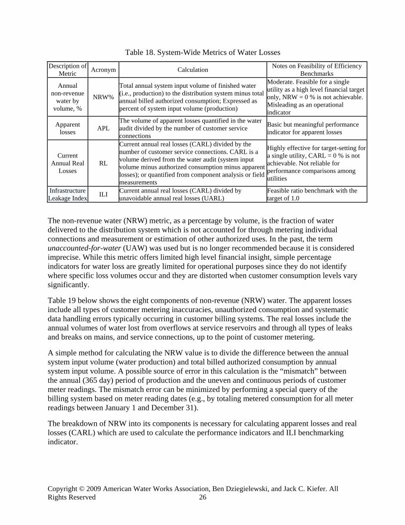
Copyright © 2009 American Water Works Association, Ben Dziegielewski, and Jack C. Kiefer. All Rights Reserved 26
Table 18. System-Wide Metrics of Water Losses
Description of Metric Acronym Calculation Notes on Feasibility of Efficiency
Benchmarks
Annual non-revenue
water by volume, %
NRW%
Total annual system input volume of finished water (i.e., production) to the distribution system minus total annual billed authorized consumption; Expressed as percent of system input volume (production)
Moderate. Feasible for a single utility as a high level financial target only, NRW = 0 % is not achievable. Misleading as an operational indicator
Apparent losses APL
The volume of apparent losses quantified in the water audit divided by the number of customer service connections
Basic but meaningful performance indicator for apparent losses
Current Annual Real
Losses RL
Current annual real losses (CARL) divided by the number of customer service connections. CARL is a volume derived from the water audit (system input volume minus authorized consumption minus apparent losses); or quantified from component analysis or field measurements
Highly effective for target-setting for a single utility, CARL = 0 % is not achievable. Not reliable for performance comparisons among utilities
Infrastructure Leakage Index ILI Current annual real losses (CARL) divided by
unavoidable annual real losses (UARL) Feasible ratio benchmark with the target of 1.0
The non-revenue water (NRW) metric, as a percentage by volume, is the fraction of water delivered to the distribution system which is not accounted for through metering individual connections and measurement or estimation of other authorized uses. In the past, the term unaccounted-for-water (UAW) was used but is no longer recommended because it is considered imprecise. While this metric offers limited high level financial insight, simple percentage indicators for water loss are greatly limited for operational purposes since they do not identify where specific loss volumes occur and they are distorted when customer consumption levels vary significantly.
Table 19 below shows the eight components of non-revenue (NRW) water. The apparent losses include all types of customer metering inaccuracies, unauthorized consumption and systematic data handling errors typically occurring in customer billing systems. The real losses include the annual volumes of water lost from overflows at service reservoirs and through all types of leaks and breaks on mains, and service connections, up to the point of customer metering.
A simple method for calculating the NRW value is to divide the difference between the annual system input volume (water production) and total billed authorized consumption by annual system input volume. A possible source of error in this calculation is the “mismatch” between the annual (365 day) period of production and the uneven and continuous periods of customer meter readings. The mismatch error can be minimized by performing a special query of the billing system based on meter reading dates (e.g., by totaling metered consumption for all meter readings between January 1 and December 31).
The breakdown of NRW into its components is necessary for calculating apparent losses and real losses (CARL) which are used to calculate the performance indicators and ILI benchmarking indicator.
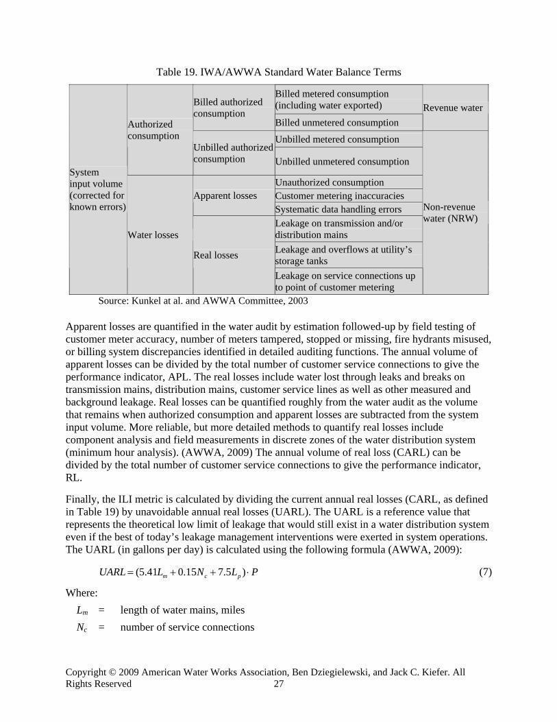
Copyright © 2009 American Water Works Association, Ben Dziegielewski, and Jack C. Kiefer. All Rights Reserved 27
Table 19. IWA/AWWA Standard Water Balance Terms
Billed metered consumption (including water exported) Billed authorized
consumption Billed unmetered consumption
Revenue water
Unbilled metered consumption Authorized consumption
Unbilled authorized consumption Unbilled unmetered consumption
Unauthorized consumption Customer metering inaccuracies Apparent losses Systematic data handling errors Leakage on transmission and/or distribution mains Leakage and overflows at utility’s storage tanks
System input volume (corrected for known errors)
Water losses
Real losses
Leakage on service connections up to point of customer metering
Non-revenue water (NRW)
Source: Kunkel at al. and AWWA Committee, 2003
Apparent losses are quantified in the water audit by estimation followed-up by field testing of customer meter accuracy, number of meters tampered, stopped or missing, fire hydrants misused, or billing system discrepancies identified in detailed auditing functions. The annual volume of apparent losses can be divided by the total number of customer service connections to give the performance indicator, APL. The real losses include water lost through leaks and breaks on transmission mains, distribution mains, customer service lines as well as other measured and background leakage. Real losses can be quantified roughly from the water audit as the volume that remains when authorized consumption and apparent losses are subtracted from the system input volume. More reliable, but more detailed methods to quantify real losses include component analysis and field measurements in discrete zones of the water distribution system (minimum hour analysis). (AWWA, 2009) The annual volume of real loss (CARL) can be divided by the total number of customer service connections to give the performance indicator, RL.
Finally, the ILI metric is calculated by dividing the current annual real losses (CARL, as defined in Table 19) by unavoidable annual real losses (UARL). The UARL is a reference value that represents the theoretical low limit of leakage that would still exist in a water distribution system even if the best of today’s leakage management interventions were exerted in system operations. The UARL (in gallons per day) is calculated using the following formula (AWWA, 2009):
PLNLUARL pcm ⋅++= )5.715.041.5( (7)
Where: Lm = length of water mains, miles Nc = number of service connections

Copyright © 2009 American Water Works Association, Ben Dziegielewski, and Jack C. Kiefer. All Rights Reserved 28
Lp = total length of private pipe, miles (obtained by multiplying Nc by the average distance from curbstop to customer meter
P = average pressure in the system, psi
For average system pressure of 60 psi, the UARL formula indicates unavoidable losses for 1.0 psi of average system pressure of 0.09 gallons per day per mile of water mains, 0.0025 gallons per day per service connection and 0.125 gallons per day per mile of private pipe.
The ILI metric has a benchmark value of 1.0. This means that at a value of 1.0 the real losses are equal to the unavoidable losses.
Table 20 shows the metrics calculated for Philadelphia based on the IWA/AWWA water audit methodology. Note that a discernable trend of reduction in real losses is shown in the average daily volume of real losses, the RL metric and the ILI benchmark.
However, the less reliable NRW% indicator shows relatively little variation over the same time span. This occurs since Philadelphia’s customer consumption has decreased at the same time that its leakage losses have been reduced. This illustrates the limitations of percentage indicators in representing operational performance regarding water loss. The values of nonrevenue water metric are compared for five utilities in Table 21.
Table 20. Examples of Water Loss Metrics for Philadelphia
Year NRW, % Apparent loss, mgd
APL, gal/conn/day
Real loss, mgd
RL, gal/conn/day ILI
2000 33.1 18.6 33.9 70.1 127.7 12.32001 32.1 14.5 26.3 68.9 125.1 12.72002 32.2 13.1 23.9 69.2 149.8 13.12003 32.1 13.3 24.2 70.5 154.6 11.92004 35.4 11.1 22.8 72.6 132.5 12.12005 34.6 14.1 25.5 66.9 121.2 11.02006 32.2 15.1 27.4 59.2 107.3 8.92007 36.3 21.8 39.6 61.6 112.0 10.32008 32.4 19.0 35.2 53.8 96.7 8.9
Table 21. Comparison of Nonrevenue Water Metric (Percent of Production)
Year Otay Irvine Ranch Phoenix Rio
Rancho Seattle Tampa 2001 -- -- 10.7 -- 8.6 -- 2002 6.6 -- 12.5 -- 7.2 -- 2003 7.6 -- 10.4 -- 6.7 -- 2004 5.4 6.6 10.7 -- 9.8 16.3 2005 10.5 6.3 10.5 -- 6.1 11.3 2006 6.7 8.1 9.7 -- 4.8 9.3 2007 3.8 8.5 8.6 -- 4.1 15.8 2008 4.3 9.1 5.2 15.8 6.4 9.4

Copyright © 2009 American Water Works Association, Ben Dziegielewski, and Jack C. Kiefer. All Rights Reserved 29
9.2 Indoor Conservation Indices
A concept similar to unavoidable leakage can be applied to the indoor and outdoor use of water in different sectors. A ratio benchmark similar to ILI can be defined for each utility by developing an estimate of an efficient level of water use to be achieved. For example, the indoor conservation index for the single-family residential sector in a given utility can be defined as:
SFaG
SFaSF
a IUMIUMICI = (8)
Where: ICIa
SF = indoor conservation index for single-family sector as a ratio-type benchmark IUMa
SF = estimated residential single-family indoor use per account per day10
IUMaGSF = efficiency goal (G) for residential single-family indoor use per account per day
The value of IUMaGSF can be obtained by disaggregating indoor water demand into its specific
components or end uses. A rational representation of each end-use can be made using a structural end use equation of the following form (Dziegielewski, 1996):
A* ] F* K + U* SM( [ = EUj
jjiG ∑ ) (9)
where EUi
G = quantity of water in end use i representing an efficiency goal G Mj = efficiency classes of the end use (set of mechanical or design parameters) Sj = fraction of end uses within efficiency classes j =1, 2 …k U = usage rate per event (or intensity of use) in end use i K = average flow rate of leaks F = fraction of end uses with leaks (incidence of leaks) A = proportion of users with end use i in a given sector of users An application of Equation 9 to the toilet end-use in the residential sector would require the knowledge of all end-use parameters. An example of the application of this equation for the toilet end use is presented in Table 22.
The efficiency classes for toilets are defined using the typical values for the design parameter Mi of 5.5, 3.5, 1.6 and 1.28 gallons per flush . The corresponding fractions of end uses within each class under current conditions are assumed to be 0.20, 0.50, 0.30, and 0.00. Also, with a typical value of 5 flushes per person per day and average household size of 2.8 persons the usage rate for the toilets would be 14 flushes per day per home. An average leakage rate of 20 gallons per day can be assumed with the incidence of leaks of 0.15. The presence parameter for toilets is 1.0. Using the equation (9), the average quantity of the current end use of water for toilet flushing would be 48.2 gallons per account per day.
10 Depending on climate characteristics it may be appropriate to weather-normalize the estimated indoor use to account for residual seasonal use that may be present in a minimum-moth estimate of indoor use.

Copyright © 2009 American Water Works Association, Ben Dziegielewski, and Jack C. Kiefer. All Rights Reserved 30
Table 22. Example of Calculations for Toilet End Use
Symbol Parameter Description Current Goal M1 Inefficient class 1 rate 5.00 5.00 S1 Inefficient class 1 fraction 0.20 0.00 M2 Standard class 2 rate 3.50 3.50 S2 Standard class 2 fraction 0.50 0.00 M3 Efficient class 3 rate 1.60 1.60 S3 Efficient class 3 fraction 0.30 0.00 M4 Efficient class 4 rate 1.28 1.28 S4 Efficient class 4 fraction 0.00 1.00 U Intensity (or frequency) of use, fpd 14.00 14.00 K Leakage rate, gpd 20.00 20.00 F Incidence of leaks 0.15 0.15 A Presence of end use 1.00 1.00
EU End use quantity, gpad 48.2 20.9
An efficiency goal for toilet flushing may be defined by a water utility by assuming that all non-conserving and standard toilets are replaced with the 1.28 gpf model that is recommended by WaterSense®. Then, at the same intensity of use (i.e., same number of flushes per day) and the same rate and intensity of leaks, the toilet end use that represents an efficiency goal would be 20.9 gallons per account per day.
Other end uses and their efficiency goals can be estimated using similar parameters and assumptions. Once all significant indoor end uses are estimated, the total value of the indoor efficiency goal can be calculated as:
∑=n
iaGaG EUIUM
1
(10)
where, EUiaG is efficiency goal for end use i where i = 1…n.
9.2.1 Single Family Indoor Use
Table 23 shows the results of the AWWA residential end use study of a sample of single-family homes (DeOreo et al, 1999). The table compares the average rates of use at the time of the study and the estimated usage with the most efficient fixtures and appliances (M3) existing at that time. The actual average indoor use in the AWWA study was 69.3 gallons per person per day.
The efficiency goal in Table 23 represents a condition requiring the installation of water efficient fixtures and appliances and requires no change in water using behavior. For example, the average volume of water used to flush the toilet was measured to be 3.7 gallons. However, 13.9 percent of recorded flushes used approximately 1.6 gallons per flush, which was then the current efficiency standard in toilet design. If all toilet flushes would use 1.28 gallons per flush, then without changing the frequency of toilet flushing, the efficient usage goal would be 6.5 gpcd instead of the previous average of 18.5 gallons. Similar assumptions can be made for the

Copyright © 2009 American Water Works Association, Ben Dziegielewski, and Jack C. Kiefer. All Rights Reserved 31
remaining seven end uses. The efficient single-family sector indoor use goal in this example is 43.5 gpcd.
Using the average and the goal values of indoor use in Table 23, the calculated value of the ICI metric for single family indoor use can be calculated as:
59.15.433.69=== SF
cG
SFcSF
a IUMIUMICI
(11)
Table 23. Examples of Average and Efficient Levels of Indoor Residential End Uses
Purpose of Use
Average Frequency of
Use (U) (events/person/
day)
Average Usage (Mi*Si)
(gallons per event)
Average Use (EUi)
(gpcd)
Efficiency Assumption
(M3*1.0) (gallons per
event)
Efficient Use Goal
(EUiG)
(gpcd) Toilet flushing 5.05 3.7 18.5 1.28 6.5 Clothes washing 0.37 40.6 15.0 25.8 9.5 Showering 0.70 16.6 11.6 14.4 10.1 Bathing 0.05 23.8 1.2 18.6 0.9 Faucet use 17.60 0.6 10.9 0.5 9.3 Dishwashing 0.10 10.0 1.0 8.0 0.8 Leaks 0.46 20.7 9.5 20.7 4.8 Other domestic -- -- 1.6 -- 1.6 Total indoor use -- -- 69.3 -- 43.5
gpcd = gallons per person per day
It is important to note that each water utility would likely develop its own efficiency goal by selecting realistic assumptions about achieving the adoption of the efficient fixtures and appliances. Also, the intensity (U) and presence (A) of end uses may vary among different utilities.
9.2.2 Multifamily Indoor Use
The ICIMF benchmark for multifamily use can also be developed for each utility. In absence of a locally derived efficiency benchmark, an approximate benchmark value for indoor use can be derived based on the AWWA end use study by assuming different rates of presence of washing machines and dishwashers in multifamily housing units.
The national submetering study (Mayer, 2004) found that only 52 percent of apartments had a washing machine. Eighteen percent of residents without a washing machine reported washing clothes at an off-site laundry (or through other arrangements). This implies that only about 85 percent of multifamily residences are expected to have the clothes washing end use. Also, 78.8 percent of respondents reported having a dishwasher.
Table 24 shows the adjusted average indoor use per person in multifamily housing based on the AWWA end use study. The estimates in the table indicate that the average indoor use in multifamily residences would be 62.2 gpcd and the efficiency goal would be 40.3 gpcd. Accordingly the value of the ICIc
MF metric would be 62.2/40.3 or 1.54.

Copyright © 2009 American Water Works Association, Ben Dziegielewski, and Jack C. Kiefer. All Rights Reserved 32
Table 24. Examples of Average and Efficient Levels of Indoor Residential End Uses in Multifamily Sector
Purpose of Use Average
Use (EUi) (gpcd)
Average Multifamily Use (EUi)
(gpcd)
Efficient Use Goal
(EUiG)
(gpcd) Toilet flushing 18.5 18.5 6.5 Clothes washing 15.0 12.75 6.46 Showering 11.6 11.6 10.1 Bathing 1.2 1.2 0.9 Faucet use 10.9 10.9 9.3 Dishwashing 1.0 0.8 0.64 Leaks 9.5 4.8 4.8 Other domestic 1.6 1.6 1.6 Total indoor use 69.3 62.2 40.3
a MF use assumes 85 percent of clothes washing use and 80 percent of dishwasher use and 50% reduction of leaks.
9.3 Outdoor Conservation Indices
In order to define a meaningful efficiency benchmark for the OUM metric, it would be necessary to determine total irrigated area in the sector and assume an agronometric theoretical value of irrigation demand for each water utility.
According to Bennett and Hazinski (1993) a theoretical irrigation water requirement can be calculated using the following irrigation water budget formula:
AIE
KKKETWB dms ⋅⋅⋅⋅
⋅= 8.0 (12)
Where: WB = theoretical irrigation water requirement ET = reference evapotranspiration Ks = crop coefficient Km = microclimate factor Kd = canopy density IE = irrigation efficiency, typically 0.80 A = irrigated area 0.8 = assumption for supplying only 80 percent of ET
Another option is to use the method developed by the EPA’s WaterSense® Water Budget Approach
(EPA, 2009). On May 8, 2009, EPA released a revised draft of the tool (file name: WaterSense Water Budget Tool_050809.xls) in a Microsoft Excel spreadsheet format that facilitates the water budget calculation for urban landscapes. This calculation can determine how much water the designed landscape requires based on climate, plant type, and irrigation system design.

Copyright © 2009 American Water Works Association, Ben Dziegielewski, and Jack C. Kiefer. All Rights Reserved 33
According to EPA, the landscape water requirement (LWR) can be calculated for each hydrozone and the sum of these values is the LWR for the site. The LWR is based on ETo, the landscape coefficient (KL), the area of the hydrozone, the lower quarter distribution uniformity (DULQ) of the associated system, and a portion of local rainfall designated as allowable rainfall (Ra):
uaLoH CARKETRTMLWR ⋅⋅−⋅⋅= ])[( (13)
Where: LWRH = landscape water requirement for the hydrozone (gallons/month) RTM = run time multiplier, equal to 1/lower quarter distribution uniformity
(dimensionless); this factor is used to increase zone run time to account for lack of distribution uniformity within the root zone
ET = local reference evapotranspiration (inches/month) which represents the rate of evapotranspiration from an extensive surface of cool-season grass cover of uniform height of 12 centimeters (4.7 inches), actively growing, completely shading the ground, and not short of water
KL = landscape coefficient for the highest water-using plant in that hydrozone (dimensionless), this coefficient is used to modify reference ET, which includes species factor (Ks), density factor (Kd), and microclimate factor (Kmc) where KL = Ks x Kd x Kmc) but for the purposes of this tool, WaterSense is assuming Kd and Kmc are both approximately equal to one to reduce the complexity of the calculations
Ra = allowable rainfall, designated by WaterSense as 25% of the site’s peak monthly rainfall
A = area of the hydrozone (square feet) which represents the grouping of plants with similar water and environmental requirements for irrigation with one of more common station/zone valves
Cu = conversion factor (0.6233 for results in gallons/month)
For a water utility, Equation 12 could be used to determine landscape water requirements for hydrozones and then entire parcels for residential and nonresidential customers to determine average water requirements per customer in a given service area. The outdoor conservation index for single family sector would then be calculated as:
153/)153/365(
SFGs
SFaSF
a LWROUM
OCI⋅
= (14)
Where: OCIa
S = outdoor conservation index for single-family sector as a ratio-type benchmark OUMa
SF = weather-normalized residential single-family outdoor use per account per day
LWRGgsSF = efficiency goal (G) for residential single-family outdoor use per account per
day represented by average irrigation water requirement during the growing season (gs)
153 = number of calendar days during the May-September growing season.

Copyright © 2009 American Water Works Association, Ben Dziegielewski, and Jack C. Kiefer. All Rights Reserved 34
Similar calculations could be performed for landscapes in multifamily and nonresidential sectors.
Unfortunately, the detailed data and assumptions required to provide an example could not be derived for this study.
10. SUMMARY RECOMMENDATIONS
10.1 Applicability of Metrics
This examination of the potential for developing water use and conservation metrics for public water supply utilities revealed several limitations as well as some possibilities for using various metrics to track water use and monitor progress in achieving efficiency goals. Table 25 provides a list of metrics that were considered, together with brief statements on their advantages, shortcomings, and appropriate use.
Table 25. Metrics of Water Use and Conservation
Category of Metric Symbol Description Selected Advantages Selected Limitations
PQc Per capita production Good availability of data on water production
Population served defined differently by water utilities and cannot be measured accurately.
PQa Production per account Number of billed accounts known for each billing period
Cannot account for differences in the composition of water use among primary sectors.
Agg
rega
te P
rodu
ctio
n B
ased
PQea Production per “equivalent” account
Number of equivalent accounts is more precise than population served
Number of equivalent accounts depends on sectoral water use characteristics
SQa Retail sales per account Separates out system losses Cannot account for differences in the composition of water use among primary sectors.
Agg
rega
te
Met
ered
Sal
es
Bas
ed
SQea Retail sales per equivalent account
Number of billed accounts known for each billing period
Number of equivalent accounts depends on sectoral water use characteristics
AUMaS
F Annual single-family usage metric per account
Definition of single-family sector generally consistent
Influenced by seasonal and weather-sensitive components of water use
AUMaM
F Annual multifamily usage metric per account
Number of accounts available and more accurate that housing unit counts.
Large variance in number of units served per multifamily account
Dia
ggre
gate
-- S
ecto
r Sa
les B
ased
AUMaN
R Annual nonresidential usage metric per account
Number of accounts available and more accurate than employment and other counting variables.
Large variance in types of businesses and corresponding water uses
IUMaSF Indoor (nonseasonal) single
family use metric per account Indoor use is considered relatively homogenous
IUMcSF Indoor (nonseasonal) single
family use metric per capita
Scales indoor use for average number of people residing in households.
OUMaS
F Outdoor (seasonal) single family use metric per account Isolates weather-sensitive uses
Dis
aggr
egat
e --
Sec
tor
and
Seas
onal
ly B
ased
IUMaMF Indoor (nonseasonal) multi-
family use metric per account Indoor use is considered relatively homogenous
Difficulty in estimating indoor/outdoor use distinction in areas with year-round outdoor and/or cooling uses. Classification of irrigation meters can confound estimates. Regularly collected data on

Copyright © 2009 American Water Works Association, Ben Dziegielewski, and Jack C. Kiefer. All Rights Reserved 35
Category of Metric Symbol Description Selected Advantages Selected Limitations
IUMcMF Indoor (nonseasonal) multi-
family use metric per capita
Scales indoor use for average number of people residing in households.
OUMaM
F Outdoor (seasonal) multi-family use metric per account Isolates weather-sensitive uses
IUMaNR Indoor (nonseasonal) nonresi-
dential use metric per accountIndoor use perhaps less variable than sector-wide use
OUMcN
R Outdoor (seasonal) nonresi-dential use metric per account
Convenient measure of weather-sensitive uses
irrigated acreage would improve use of account-level data Heterogeneity of customers and class definitions for multifamily and nonresidential categories limits inter-utility comparisons
NRW Nonrevenue water Easily computed from commonly available data
Combines real and apparent water losses
CARL Real resource loss Focuses on real (physical) losses Does not provide any allow-ances for unavoidable leaks
Leak
age
and
Loss
ILI Infrastructure leakage index Can be used for inter-utility comparisons
Rigid formula for assessing unavoidable leaks
ICISF Indoor single-family conservation index
ICIMF Indoor multifamily conservation index
OCISF Outdoor single-family conservation index C
onse
rvat
ion
Indi
ces
OCIMF Outdoor multifamily conservation index
Ratio benchmarks with 1.0 target/goal value Can be tailored to reflect service area end use and weather characteristics Can be used for inter-utility comparisons
Indoor use measure may include outdoor uses using minimum month estimation methods Requires definition and calculation of benchmark usage rates for indoor and outdoor use Outdoor benchmark values require multiple assumptions to reflect service area characteristics
All metrics in Table 25 except the conservation indices are best suited for making comparisons of water use at a single water utility. The ILI, ICI and OCI metrics can be used (with some fundamental caution) in cross-utility comparisons.
10.2 Key Findings
The analysis and comparison of the values of different metrics for the seven case study utilities resulted is several relevant findings. The following is a summary of key findings.
1. Available water production and sales records can be used to calculate both system-wide and sector-specific metrics of water use. However, the only accurate and regularly updated measure of system size is the number of connections or customer accounts. Other measures of system size such as population served, number of housing units, or the number of employees are not precisely defined and at best are updated only on annual basis. For this reason the commonly used metric representing annual production per capita, or GPCD, should not be used as a benchmark.

Copyright © 2009 American Water Works Association, Ben Dziegielewski, and Jack C. Kiefer. All Rights Reserved 36
2. Useful sector-specific metrics can be defined and calculated precisely. However, each water utility uses a different system for classifying customer accounts. This makes it difficult to consolidate the existing customer types into user sectors such as residential, commercial, industrial, and institutional and others. Even if such sectoral groupings are made, their customer characteristics and composition may vary across different utilities.
3. Both system-wide and sector-wide metrics can be used to track water usage per account over time. However, the year-to-year changes of the values of each metric have to be carefully interpreted. These changes may have different causes; oftentimes changes in water use that are related to weather conditions and/or the composition of water users can mask or overwhelm changes in use resulting from water conservation efforts.
4. No metrics of water use (measured in absolute terms) should be used for judging relative water use efficiency across different utilities. Different utilities will likely display uniqueness in terms of the climate and composition of demands in their respective service areas. Only ratio metrics such as the Infrastructure Leakage Index (ILI) with a benchmark value of 1.0 could be used (although with some caution) for inter-utility comparisons.
5. Ratio-type benchmarks can be formulated for different components of sectoral water use. These benchmarks can be compared across different utilities; however the absolute benchmarks on which such ratios are based should be unique to each utility. For example, the proposed Indoor Conservation Index (ICI) would be based on an efficiency goal of indoor use that would take into account specific conditions of each utility.
6. A promising way for developing metrics, absolute benchmarks, and efficiency goals is to disaggregate sectoral demands into specific end uses. End-use specific benchmark values can be formulated based on technological standards and assumptions regarding the intensity or frequency of use. Measurement of water use at an end-use level would naturally improve the indoor and outdoor metrics discussed in this report. Unfortunately, highly disaggregated end use data are not available in most water utilities.
10.3 Recommendations
The results of this study lend support to two major recommendations: one pertains to the data and water use records and the other to the development of supportive information for the conservation benchmarks.
1. Significant improvements in the ability of water utilities to reduce definitional noise and monitor water usage rates over time would be achieved if the water supply industry adopted a standard set of customer types and customer classification procedures. This ability would be enhanced further if water utilities collected and maintained additional characteristics for each customer. These would depend on customer type and could include such measurements as irrigated area, number of dwelling units, number of employees and the presence of specific end uses such as swimming pools or evaporative coolers.11
11 The authors of this report and some members of the study review committee are currently developing a tailored collaboration study approach for determining information management needs for utility planning.
Copyright © 2009 American Water Works Association, Ben Dziegielewski, and Jack C. Kiefer. All Rights Reserved 37
2. The suggested conservation indices for indoor and outdoor use (i.e., ratio benchmarks ICI and OCI) should be further investigated through a pilot study in a sample of water utilities. The indoor component of the study could include end-use measurement similar to the 1999 end use study conducted by AWWA for both single family and multifamily sectors, in particular to improve upon the limitations of the minimum-month method for estimating indoor use, as well as to establish baseline conditions and conservation benchmarks. The outdoor component of the study could include measurement of irrigated areas and watering requirements through advanced remote sensing techniques and on-site measurements of actual water use for irrigation and outdoor purposes in a sample of residential and nonresidential parcels.
NOTATION
Acronyms for metrics:
PQ = water production quotient SQ = water sales quotient UM = usage metric CI = conservation index
Dimensions of water use (added in front of the acronyms for metrics):
A = annual average (daily) water production, sales or usage I = indoor (nonseasonal) water use O = outdoor (seasonal) water use
Sectors of water users (added as a superscript after the acronyms for metrics):
SF = single-family sector MF = multifamily sector NR = nonresidential sector
Scaling variables (added as a subscript after the acronyms for metrics):
c = per capita based on population served or number of residents a = per account based on the number of billed accounts ea = equivalent account
also
G = goal or benchmark value

Copyright © 2009 American Water Works Association, Ben Dziegielewski, and Jack C. Kiefer. All Rights Reserved 38
REFERENCES
AWWA. 2009. M36 Publication. Water Audits and Loss Control Programs 3rd Edition.
Baumann, D. D., J. J. Boland, and J. H. Sims. 1984. Water Conservation: The Struggle Over Definition, Water Resources Research, 20(4), 428–434.
Bennett, R., and Hazinski, H. 1993. Water-Efficient Landscape Guidelines. AWWA.
DeOreo, W.B., P.W. Mayer, E.M. Opitz, B. Dziegielewski, J.C. Kiefer, W.Y. Davis, and J.O. Nelson. 1999. Residential End Uses of Water: Final Report. AWWA Research Foundation. Denver, Colorado.
Dziegielewski, B., J. C. Kiefer, W. DeOreo, P. Mayer, E. M. Opitz, G. A. Porter, G. L. Lantz, and J. O. Nelson. 2000. Commercial and Institutional End Uses of Water. Published by AWWA Research Foundation and American Water Works Association with Cooperation of the U.S. Bureau of Reclamation, Denver, Colorado (September 2000). Catalog No.90806. 264 pp. ISBN 1-58321-035-0.
Dziegielewski, B. 1996. Feasibility of Water Efficiency Standards. AWWA Proceedings Conserv96. Orlando, Florida.
EPA (2009) Revised WaterSense®
Water Budget Approach Accessed at http://www.epa.gov/watersense/docs/home_waterbudget508.pdf on October 30, 2009
Gonzalez, Yassert A., Jay W. Yingling. 2008. How to Quickly Calculate Required and Optional Population Served Estimates using data found in District and Utility Demographics. Planning Department, Southwest Florida Water Management District June 26, 2008. http://www.swfwmd.state.fl.us/data/demographics/quick_population_served_estimates.pdf
Kunkel, G. et al. "Applying Worldwide Best Management Practices in Water Loss Control". Water Loss Committee Report. Journal AWWA, 95(8):65, 2003
Mayer, Peter W., Erin Towler, William B. DeOreo, Erin Caldwell, Tom Miller, Edward R. Osann, Elizabeth Brown, Peter J. Bickel, Steven B. Fisher. (2004) National Multiple Family Submetering and Allocation Billing Program Study. Aquacraft, Inc. and the East Bay Municipal Utility District
New Mexico Office of the State Engineer Gallons Per Capita Per Day Calculator
Instruction Module. For 2.04 Beta Version, March 2009
Thornthwaite, C.W. & Mather, J.R. (1955) The Water Balance. Publ. in Climatology, vol.8, no.l. C.W. Thornthwaite & Associates, Centerton, New Jersey

Copyright © 2009 American Water Works Association, Ben Dziegielewski, and Jack C. Kiefer. All Rights Reserved 39
APPENDIX A
CASE STUDY TABLES

Copyright © 2009 American Water Works Association, Ben Dziegielewski, and Jack C. Kiefer. All Rights Reserved 40
CASE #1 OTAY WATER DISTRICT, CALIFORNIA
Table O1. Annual Production (MG), Sales (CCF) and Billed Accounts Data for Otay Water District, California
Description 2002 2003 2004 2005 2006 2007 2008 C.V. TrendPopulation Served 149,132 160,252 171,373 177,634 183,895 190,156 196,416 9.5 4.48Production (Potable) 36,856 35,857 39,378 39,932 41,740 39,359 36,821 5.5 0.86Production (Recycled) 1,119 1,209 1,275 1,227 1,228 1,206 1,202 3.9 0.58Purchase (Recycled) 2,759 3,524 17.2 27.74Total metered sales: 15,456,498 14,916,586 16,761,288 16,048,790 17,459,150 18,155,769 17,324,974 7.0 2.80Total Residential 9,147,579 9,172,475 9,646,201 9,983,730 10,778,272 11,080,760 10,475,434 7.6 3.24 Single-family 8,145,112 8,106,525 8,447,007 8,837,155 9,428,653 9,655,479 9,045,979 6.9 2.79 Multifamily 1,002,467 1,065,950 1,199,194 1,146,575 1,349,619 1,425,281 1,429,455 14.0 6.51Commercial 759,669 744,443 1,527,960 861,316 871,767 922,899 939,562 28.2 0.91Irrigation 2,470,244 2,027,714 2,231,341 2,038,685 2,158,727 2,316,057 2,217,028 7.0 -0.41Agricultural 89,272 77,013 68,852 53,043 50,344 57,972 48,502 24.1 -9.85Public 919,553 919,033 901,744 911,968 963,747 960,105 946,271 2.6 0.86Recycled water 1,141,825 1,284,886 1,608,699 1,639,477 1,806,359 1,989,596 2,020,373 20.4 9.94Construction 928,356 686,364 766,060 412,846 659,057 639,370 553,672 24.3 -6.99Fire Services 4,608 10,185 0 52 10,615 4,012 95.0 -0.95Sales to other agencies 50 245 147,725 170,825 178,395 120,120 79.8 55.85Total billed accounts: 40,726 42,802 45,233 47,072 48,283 48,289 48,227 6.6 2.90Total Residential 37,652 39,515 41,763 43,386 44,344 44,307 44,175 6.3 2.73 Single-family 36,931 38,785 41,017 42,622 43,557 43,506 43,363 6.3 2.74 Multifamily 722 731 746 764 787 801 812 4.6 2.13Commercial 989 991 1,040 1,086 1,135 1,154 1,183 7.3 3.03Irrigation 1,022 989 986 1,082 1,120 1,170 1,188 7.7 2.55Agricultural 24 38 33 32 32 30 24 16.6 -2.11Public 204 216 216 222 228 232 233 4.7 2.15Recycled water 182 324 470 484 557 589 628 34.3 17.71Construction 226 266 266 252 240 201 162 16.6 -5.33Fire Services 426 462 460 526 626 604 633 16.3 7.55Sales to other agencies 1 1 1 1 1 1 1 0.0 0.00

Copyright © 2009 American Water Works Association, Ben Dziegielewski, and Jack C. Kiefer. All Rights Reserved 41
Table O2. Calculated Metrics Using the Number of Accounts and Population Served as Normalizing Variables for Otay Water District, California
Description 2002 2003 2004 2005 2006 2007 2008 C.V. 2002-2008Trend
Per account metrics (gpad): Total Residential 480 483 486 488 490 493 495 1.1 0.49 Single-family 435 436 436 436 436 437 437 0.1 0.05 Multifamily 2,858 3,010 3,155 3,294 3,427 3,555 3,677 9.0 4.27Commercial 1,908 1,923 1,849 1,786 1,724 1,712 1,685 5.4 -2.39Irrigation 4,484 4,613 4,611 4,183 4,024 3,836 3,761 8.5 -3.60Agricultural 5,220 4,915 4,598 4,267 3,921 3,561 3,184 17.3 -7.84Public 8,966 8,844 8,728 8,616 8,510 8,407 8,309 2.7 -1.26Recycled water 9,636 8,512 7,788 7,283 6,910 6,624 6,398 15.2 -6.62Construction 6,165 6,087 6,001 5,906 5,799 5,680 5,545 3.8 -1.73Fire Services 23 21 19 18 16 15 14.9 -7.73Sales to other agencies 41,368 109,165 176,962 244,759 312,557 380,354 60.2 55.85All sales/all accounts 745 744 743 742 742 741 740 0.2 -0.10Per capita metrics (in gpcd): Per capita production 227.3 206.5 211.8 206.9 208.6 203.4 188.8 5.5 -2.13Total sales per capita 204.4 200.2 196.3 192.6 189.3 186.3 183.4 3.9 -1.79Residential sales per capita 122.0 120.2 118.7 117.2 115.9 114.7 113.5 2.6 -1.19Commercial sales per capita 12.4 11.9 11.5 11.1 10.7 10.4 10.0 7.5 -3.43Construction sales per capita 10.8 9.7 8.7 7.7 6.9 6.1 5.4 24.7 -11.21Nonrevenue water (%) 6.6 7.6 5.4 10.5 6.7 3.8 4.3 35.3 -7.18

Copyright © 2009 American Water Works Association, Ben Dziegielewski, and Jack C. Kiefer. All Rights Reserved 42
Table O3. Metrics Based on Socioeconomic Data for Otay California
Description 2004 2008 Population served 171,373 196,416 Employment (civilian) 38,778 52,838 SF housing units 44,646 44,830 MF units 9,394 16,388 SF persons per households 3.445 3.490 SF population 153,805 156,457 MF population 17,568 39,960 SF sales per housing unit 393.2 435.9 MF sales per housing unit 251.8 182.8 SF sales per capita 114.1 124.9 MF sales per capita 134.7 75.0 NR sales per employee 139.2 95.0
Table O4. Monthly and Seasonal Single-Family Residential Usage Rates in Otay, California.
Month 2002 2003 2004 2005 2006 2007 2008Per account use (gpad): January 330.0 318.7 297.5 265.9 391.2 343.7 318.4February 363.4 387.6 307.8 303.6 378.0 362.2 280.7March 359.0 268.7 223.1 248.4 332.0 299.1 271.4April 394.6 377.0 339.6 316.9 284.9 370.0 380.9May 427.2 358.8 409.7 419.0 337.0 385.3 466.8June 543.0 490.2 564.5 520.1 463.5 588.5 481.0July 536.7 508.0 511.6 505.2 567.1 556.2 506.8August 588.0 531.4 595.1 556.3 564.9 553.5 558.4September 594.4 582.5 610.3 552.9 598.6 643.5 544.0October 477.6 508.9 494.9 510.0 514.8 487.1 480.2November 431.0 459.7 366.4 428.9 448.0 494.3 470.7December 370.5 340.2 320.5 433.7 437.3 373.0 362.9Annual average 452.0 428.3 422.0 423.9 443.6 454.8 427.5Minimum month 330.0 268.7 223.1 248.4 284.9 299.1 271.4Percent nonseasonal 72.7 62.8 52.7 58.5 63.2 66.7 60.5Percent seasonal 27.3 37.2 47.3 41.5 36.8 33.3 39.5

Copyright © 2009 American Water Works Association, Ben Dziegielewski, and Jack C. Kiefer. All Rights Reserved 43
Table O5. Monthly and Seasonal Multifamily Residential Usage Rates in Otay, California.
Month 2002 2003 2004 2005 2006 2007 2008Per account use (gpad): January 2,557 2,615 3,127 2,628 3,316 3,431 3,489February 2,752 2,933 3,356 3,168 3,106 3,311 3,404March 2,419 2,458 2,793 2,801 2,900 3,066 3,041April 2,724 2,711 3,220 2,825 2,492 3,290 3,426May 2,640 2,671 3,129 3,111 2,694 3,130 3,506June 3,051 3,158 3,697 3,460 3,212 4,168 3,736July 2,938 3,111 3,180 3,171 3,517 3,775 3,605August 3,170 3,228 3,638 3,324 3,719 3,809 3,939September 3,360 3,480 3,761 3,244 3,947 4,420 4,257October 2,876 3,328 3,353 3,255 3,667 3,845 3,806November 2,939 3,177 3,292 2,945 3,482 4,005 3,687December 2,739 3,011 3,021 2,724 3,013 3,474 3,390Annual average 2,846 2,990 3,296 3,055 3,250 3,647 3,608Minimum month 2,419 2,458 2,793 2,628 2,492 3,066 3,041Percent nonseasonal 86.4 83.4 85.7 85.9 75.7 82.4 85.5Percent seasonal 13.6 16.6 14.3 14.1 24.3 17.6 14.5
Table O6. Monthly and Seasonal Nonresidential (Commercial/Public/Construction) Usage Rates in Otay, California.
Month 2002 2003 2004 2005 2006 2007 2008Per account use (gpad): January 2,537 2,617 4,234 2,284 2,749 2,728 2,222February 3,075 3,045 4,534 2,189 2,644 2,851 2,473March 3,221 2,576 4,218 2,008 2,476 2,431 2,057April 3,797 2,599 4,762 2,465 2,290 2,637 2,540May 4,211 2,758 6,520 3,622 2,450 2,744 3,027June 4,487 3,518 3,547 3,684 3,281 3,791 3,349July 4,335 3,585 3,739 4,013 3,647 3,803 3,802August 4,249 3,800 4,279 4,293 3,862 3,623 4,035September 4,382 4,080 4,376 2,920 4,314 4,372 3,889October 3,686 4,093 5,786 2,706 3,797 3,674 3,900November 3,864 3,619 3,248 2,451 3,332 2,587 3,542December 3,260 2,867 2,478 1,720 3,259 3,836 3,098Annual average 3,766 3,271 4,304 2,863 3,188 3,258 3,169Minimum month 2,537 2,576 2,478 1,720 2,290 2,431 2,057Percent nonseasonal 66.4 78.0 60.7 62.4 69.6 76.2 65.4Percent seasonal 33.6 22.0 39.3 37.6 30.4 23.8 34.6

Copyright © 2009 American Water Works Association, Ben Dziegielewski, and Jack C. Kiefer. All Rights Reserved 44
Table O7. System-wide Production, Consumption and Losses in Otay WD
Description Units 2006 2008Water imported: acre-ft/yr 42,329.50 43,260.80Water exported: acre-ft/yr 393.80 281.40WATER SUPPLIED: acre-ft/yr 41,935.70 42,979.40AUTHORIZED CONSUMPTION Billed metered: acre-ft/yr 37,940.30 40,350.70Billed unmetered: acre-ft/yr 58.80 135.40Unbilled metered: acre-ft/yr 295.80 221.40Unbilled unmetered: acre-ft/yr 524.20 537.24AUTHORIZED CONSUMPTION: acre-ft/yr 38,819.10 41,244.74WATER LOSSES acre-ft/yr 3,116.60 1,734.66Apparent Losses Unauthorized consumption: acre-ft/yr 104.84 107.45Customer metering inaccuracies: acre-ft/yr 3.82 4.06Systematic data handling errors: acre-ft/yr 58.80 135.40Apparent Losses: acre-ft/yr 167.46 246.91Real Losses = Water Losses - Apparent Losses: acre-ft/yr 2,949.14 1,487.75WATER LOSSES: acre-ft/yr 3,116.60 1,734.66NON-REVENUE WATER: acre-ft/yr 3,936.60 2,493.30Length of mains: miles 750.00 750.00Number of active and inactive service connections: 46,874.00 46,874.00Connection density: conn./mile main 62.50 62.50Average length of customer service line: ft 22.00 22.00Average operating pressure: psi 95.00 95.00Apparent Losses per service connection per day: gallons/connection/day 3.19 4.70Real Losses per service connection per day: gallons/connection/day 56.17 28.34Real Losses per service connection per day per psi pressure:
gallons/connection/day/psi 0.59 0.30
Unavoidable Annual Real Losses (UARL): million gallons/year 435.29 435.29Infrastructure Leakage Index (ILI) [Real Losses/UARL]:
-- 2.21 1.11

Copyright © 2009 American Water Works Association, Ben Dziegielewski, and Jack C. Kiefer. All Rights Reserved 45
CASE #2 IRVINE RANCH WATER DISTRICT, CALIFORNIA
Table I1. Reported Production and Sales Data for Irvine Ranch Water District, California
Description 2004-05 2005-06 2006-07 2007-08 2008-09 C.V. Trend Production (AF) 86,906.1 89,279.4 100,721.3 98,978.2 98,826.7 6.7 3.60Metered Sales (AF) to: Total Residential 30,689.4 31,851.3 34,442.9 34,307.1 34,799.8 5.5 3.27 Single-family 26,103.5 26,739.6 29,187.0 28,738.3 29,131.7 5.2 2.92 Multifamily 4,585.9 5,111.7 5,255.9 5,568.8 5,668.1 8.2 5.15Commercial 7,663.1 8,095.4 8,772.0 8,824.3 8,524.7 5.9 2.97Industrial 6,047.3 5,754.4 5,441.7 5,358.9 5,009.6 7.2 -4.39Governmental 2,841.8 2,795.1 2,474.2 2,588.3 2,571.0 5.9 -2.78Irrigation Agricultural 7,222.7 8,225.5 8,660.3 7,559.5 7,856.0 7.1 0.76Urban 22,806.9 23,897.5 29,302.0 28,701.2 27,888.2 11.2 5.83Public 0.0 0.0 0.0 0.0 0.0 Combined nonresidential 564.0 897.7 835.9 808.2 279.5 37.8 -9.38Wholesale to other agenc. 3,309.3 2,145.2 2,647.7 2,399.6 2,945.0 17.0 -1.75Total sales 81,144.5 83,662.1 92,576.7 90,547.1 89,873.8 5.6 2.82

Copyright © 2009 American Water Works Association, Ben Dziegielewski, and Jack C. Kiefer. All Rights Reserved 46
Table I2. Customer Classification and Number of Accounts in Irvine Ranch, California
Customer Classification/Fiscal Year 2004-05
2005-06
2006-07
2007-08
2008-09 C.V. Trend
Total Residential Single-family (10, 11, 12, 18, 71, 91) 46,891 48,148 50,059 50,668 51,542 3.8 2.42Separately Metered Condo (13, 16) 22,133 22,770 23,292 23,804 24,030 3.3 2.10Separately Metered Apt (14, 17) 5,345 5,345 5,345 5,345 5,346 0.0 0.00Master Metered Condo - Multifamily (80, 83) 732 804 830 838 850 5.8 3.40Master Metered Apts - Multifamily (81, 82) 1,489 1,490 1,527 1,600 1,687 5.4 3.30Other Commercial - Potable (20, 22, 72, 92) 1,821 3,723 4,258 4,632 4,840 31.5 20.76Commercial - Untreated (21, 23) 3 3 2 2 2 25.4 -13.67Commercial - HOA (27) Commercial (28) Commercial - Recycled Water (29) 13 13 19 36 48 60.0 56.79Industrial - Potable (30,38) 880 876 870 865 858 1.0 -0.62Industrial - Recycled (32) 1 1 2 2 1 34.5 12.26Public Authority (40, 46, 47, 48, 94) 221 227 252 262 269 8.7 5.50Irrigation - Potable (60, 76, 93) 1,751 1,765 1,783 1,799 1,811 1.4 0.87Irrigation - Untreated (61) 106 134 234 214 167 31.4 12.91Irrigation - Recycled (62, 63, 65) 3,636 3,801 3,925 4,202 4,374 7.5 4.84Irrigation - Lake Fill (64) Ag - Potable (66) 21 21 23 23 19 7.7 -1.47Ag - Untreated (67, 69) 40 35 35 35 31 8.5 -4.78Ag - Recycled (68) 17 13 13 14 19 17.5 2.79Construction - Temporary Potable (50, 75, 95) 181 212 261 197 126 25.2 -6.20Construction - Temporary Recycled (51) 5 4 4 3 2 30.6 -16.97Hydrants (90, 98) 2,294 2,429 2,572 2,756 2,931 9.8 6.40Wholesale Water to Other Agencies Total billed accounts 87,579 91,813 95,306 97,297 98,953 4.8 3.05

Copyright © 2009 American Water Works Association, Ben Dziegielewski, and Jack C. Kiefer. All Rights Reserved 47
Table I3. Summary of Billed Accounts in Irvine Ranch Water District, California.
Fiscal Year/ Customer Classification
2004-05
2005-06
2006-07
2007-08 2008-09 C.V. Trend
Total Residential 76,590 78,557 81,053 82,255 83,455 3.5 2.19 Single-family 74,368 76,263 78,696 79,817 80,918 3.4 2.16 Multifamily 2,221 2,294 2,357 2,438 2,537 5.2 3.33Commercial 1,834 3,736 4,277 4,668 4,887 31.6 20.93Industrial 880 876 870 865 858 1.0 -0.62Governmental 221 227 252 262 269 8.7 5.50Irrigation Agricultural 78 70 71 72 69 5.2 -2.24 Urban 5,492 5,700 5,943 6,215 6,352 6.0 3.84Combined nonresidential 186 216 266 200 128 25.0 -6.39Total Sales 85,281 89,380 92,731 94,536 96,019 4.7 2.95
Table I4. Calculated Metrics Using the Number of Accounts as Normalizing Variable
Fiscal Year/ Customer Classification
2004-05
2005-06
2006-07
2007-08
2008-09 C.V. Trend
Water Use per Account (gpad) Total Residential 358 362 379 372 372 2.4 1.08 Single-family 313 313 331 321 321 2.3 0.77 Multifamily 1,843 1,989 1,990 2,039 1,994 3.8 1.80Commercial 3,729 1,935 1,831 1,688 1,557 41.7 -20.42Industrial 6,134 5,868 5,587 5,531 5,211 6.2 -3.79Governmental 11,480 11,001 8,759 8,831 8,525 14.4 -8.05Irrigation Agricultural 82,315 105,532 109,407 94,168 101,398 10.9 2.76 Urban 3,708 3,743 4,402 4,123 3,920 7.2 2.04Combined nonresidential 2,714 3,719 2,811 3,609 1,949 24.5 -5.41Total sales/total accounts 849 836 891 855 836 2.7 -0.10

Copyright © 2009 American Water Works Association, Ben Dziegielewski, and Jack C. Kiefer. All Rights Reserved 48
Table I5. Monthly and Seasonal Single-Family Residential Usage Rates in Irvine Ranch, California.
Month 2004-5 2005-6 2006-7 2007-8 2008-9 Per account use (gpad): January 250.0 266.7 280.1 259.2 244.6February 232.2 267.9 274.6 224.6 253.2March 237.7 255.5 275.4 251.6 243.6April 275.3 225.5 289.6 297.4 297.2May 306.6 265.2 305.9 325.1 321.8June 355.6 330.1 362.0 347.1 340.4July 375.9 375.1 384.5 378.9 379.4August 425.1 375.6 382.4 367.2 363.4September 389.5 378.0 389.1 386.2 370.4October 381.4 353.8 348.2 338.3 354.0November 265.1 303.7 321.0 324.2 329.9December 279.0 292.1 287.6 286.2 286.8Annual average 313.4 313.0 331.1 321.4 321.4Minimum month 232.2 225.5 274.6 224.6 243.6Percent nonseasonal 75.3 73.9 84.8 71.3 77.4Percent seasonal 24.7 26.1 15.2 28.7 22.6
Table I6. Monthly and Seasonal Multifamily Residential Usage Rates in Irvine Ranch, California.
Month 2004-5 2005-6 2006-7 2007-8 2008-9 Per account use (gpad): January 1,743 1,860 1,915 1,956 1,853February 1,657 1,869 1,932 1,868 1,857March 1,796 1,863 1,958 1,899 1,862April 1,730 1,781 1,767 1,984 1,897May 1,800 1,865 1,909 1,956 1,910June 1,832 2,045 2,114 2,032 1,988July 2,061 2,092 1,648 2,100 2,083August 2,020 1,991 2,017 2,017 2,011September 1,925 2,079 2,141 2,079 2,065October 1,995 2,076 2,046 2,091 2,040November 1,744 1,986 2,027 2,008 1,985December 1,841 1,923 1,962 2,023 1,945Annual average = (a) 1,843 1,989 1,990 2,039 1,994Minimum month = (b) 1,657 1,781 1,648 1,868 1,853Percent nonseasonal, (b)/(a) 89.9 89.5 82.8 91.6 92.9Percent seasonal, 100-(b)/(a) 10.1 10.5 17.2 8.4 7.1

Copyright © 2009 American Water Works Association, Ben Dziegielewski, and Jack C. Kiefer. All Rights Reserved 49
Table I7. Monthly and Seasonal Nonresidential Usage Rates in Irvine Ranch, California.
Month 2004-5 2005-6 2006-7 2007-8 2008-9 Per account use (gpad): January 2,422 2,399 2,178 2,054 1,698February 2,465 2,571 2,421 2,115 1,972March 2,466 2,500 2,379 2,161 1,939April 2,489 2,285 2,435 2,420 2,256May 2,832 2,532 2,603 2,574 2,338June 3,241 3,105 2,929 2,609 2,440July 3,315 3,177 2,986 2,922 2,784August 3,867 3,250 3,249 2,905 2,694September 3,465 3,775 3,253 3,084 2,683October 3,496 3,177 2,869 2,811 2,583November 2,866 2,787 2,771 2,670 2,507December 2,730 2,743 2,482 2,506 2,158Annual average = (a) 2,959 2,911 2,762 2,618 2,381Minimum month = (b) 2,422 2,285 2,178 2,054 1,698Percent nonseasonal, (b)/(a) 81.8 78.5 78.9 78.5 71.3Percent seasonal, 100-(b)/(a) 18.2 21.5 21.1 21.5 28.7

Copyright © 2009 American Water Works Association, Ben Dziegielewski, and Jack C. Kiefer. All Rights Reserved 50
CASE #3 -- PHOENIX WATER SERVICES DEPARTMENT, ARIZONA
Table P1. Number of Accounts by Customer Category in Phoenix Water Services Department, Arizona Customer Type - Description 2001 2002 2003 2004 2005 2006 2007 2008 C. V. Trend 1 Commercial -unit - pools, landsc. sprinklers, warehouse, vacant lots, public restrooms 11,717 11,908 12,051 12,211 12,443 12,634 12,820 13,048 3.8 1.54
1 Family residence 305,827 310,348 316,848 325,119 335,810 345,904 352,959 354,101 5.8 2.37 1 Family residence & 2 commercial units 17 16 15 16 16 16 16 16 3.1 -0.20 1 Family residence and 1 commercial unit 446 446 442 439 434 429 420 412 2.9 -1.13 2 Commercial units 494 495 496 497 494 488 484 482 1.2 -0.41 2 Family residences - duplex 4,046 4,042 4,047 4,048 4,040 4,030 4,006 3,966 0.7 -0.24 2 Family residences & 1 commercial unit 56 56 55 55 52 53 52 51 3.9 -1.51 2-1 Family residences 665 665 664 666 661 654 650 639 1.4 -0.52 3 Commercial units 297 298 301 304 304 304 301 299 0.9 0.18 3 Family residences - triplex 1,662 1,659 1,655 1,647 1,674 1,691 1,689 1,681 1.0 0.30 3-1 Family residences 86 87 87 86 85 83 82 82 2.3 -0.87 4 Stores 776 788 794 796 799 796 796 798 0.9 0.30 Apartments - 4 units or more, condos 8,375 8,505 8,586 8,670 8,752 8,813 8,866 8,918 2.2 0.88 Car wash 112 116 119 118 118 121 126 130 4.7 1.82 Church rate 886 896 902 911 913 907 911 917 1.1 0.40 City of phoenix 592 607 618 625 638 658 664 682 4.9 2.00 Federal 46 47 47 46 46 48 50 49 3.1 0.94 Fire hydrant meter 525 480 507 555 623 762 758 582 18.1 5.41 Governments 225 226 229 226 225 223 220 220 1.4 -0.44 Heavy industry 174 175 180 185 187 186 186 183 2.9 0.95 Hotel, motel 415 414 418 419 414 410 404 406 1.3 -0.41 Institutions 358 358 361 362 362 365 370 377 1.7 0.66 Killed or inactive taps 455 360 273 163 95 31 7 4 99.1 -176.77 Laundry - commercial 50 49 49 49 48 47 51 51 2.7 0.26 Laundry - self service 75 76 76 79 78 79 82 81 3.0 1.16 Mortuary 27 27 27 27 26 26 26 26 1.9 -0.66 Office/bank building (non-dining), medical building, nursing home 1,371 1,379 1,385 1,393 1,397 1,407 1,416 1,426 1.3 0.55
Restaurant, bakery 1,371 1,403 1,425 1,441 1,447 1,460 1,469 1,478 2.5 0.99 Schools 747 780 811 839 856 881 903 928 7.3 3.04 Service station, auto repair 647 644 640 633 628 626 619 617 1.8 -0.72 Trailer courts 313 312 311 309 306 301 296 295 2.3 -0.92 Irrigation 7,507 7,918 8,302 8,689 9,143 9,524 9,909 10,465 11.4 4.79 All user types (sum) 350,357 355,580 362,720 371,620 383,113 393,956 401,605 403,412 5.5 2.26

Copyright © 2009 American Water Works Association, Ben Dziegielewski, and Jack C. Kiefer. All Rights Reserved 51
Table P2. Average Water Use per Account (GPAD) by Customer Category in Phoenix Water Services Department, Arizona Customer Type - Description 2001 2002 2003 2004 2005 2006 2007 2008 C. V. Trend 1 Commercial -unit - pools, landscaping, sprinklers, warehouse, vacant lots, public restrooms
1,622 1,578 1,544 1,516 1,492 1,555 1,579 1,419 4.1 -1.09
1 Family residence 452 457 430 413 397 403 401 372 6.9 -2.65 1 Family residence & 2 commercial units 603 538 487 538 453 445 444 428 12.5 -4.53 1 Family residence and 1 commercial unit 648 632 611 561 544 542 544 504 8.9 -3.43 2 Commercial units 882 874 902 904 786 813 814 759 6.6 -2.17 2 Family residences - duplex 583 568 543 511 498 501 486 439 9.1 -3.55 2 Family residences & 1 commercial unit 963 783 803 681 642 700 586 586 17.8 -6.49 2-1 Family residences 733 732 675 646 615 623 617 572 8.9 -3.41 3 Commercial units 1,415 1,301 1,305 1,313 1,277 1,260 1,247 1,140 6.0 -2.19 3 Family residences - triplex 863 834 795 736 694 703 680 625 11.1 -4.36 3-1 Family residences 999 1,046 972 963 960 918 915 815 7.2 -2.62 4 Stores 2,957 2,896 2,775 2,701 2,625 2,617 2,547 2,388 6.9 -2.75 Apartments - 4 units or more, condos 4,532 4,392 4,235 4,096 4,025 4,041 3,908 3,655 6.7 -2.64 Car wash 6,119 6,275 5,941 5,909 6,421 6,643 6,416 5,613 5.5 -0.04 Church rate 1,530 1,507 1,429 1,328 1,307 1,340 1,353 1,229 7.5 -2.70 City of phoenix 6,590 5,865 5,312 5,584 5,659 5,426 5,607 5,053 8.1 -2.43 Federal 4,320 4,402 3,969 3,777 4,222 3,816 3,917 3,643 6.9 -2.11 Fire hydrant meter 5,592 4,774 4,150 4,240 3,811 4,574 4,427 4,537 11.7 -2.16 Governments 8,922 9,037 8,952 8,587 7,442 7,128 6,984 6,846 12.2 -4.62 Heavy industry 45,950 43,344 42,253 40,943 40,842 41,657 42,135 39,715 4.5 -1.45 Hotel, motel 9,676 9,337 9,890 9,873 10,379 10,715 10,604 9,879 4.7 1.28 Institutions 4,577 4,634 4,713 4,582 4,460 4,295 4,173 3,845 6.6 -2.35 Killed or inactive taps 1,017 1,048 1,029 1,180 2,340 2,449 2,409 1,219 42.7 11.30 Laundry - commercial 6,769 6,890 6,827 6,690 7,386 7,481 6,783 6,541 4.8 0.09 Laundry - self service 8,690 8,652 8,331 8,157 8,508 8,678 7,910 6,630 8.4 -2.41 Mortuary 1,485 1,642 1,650 1,656 1,694 1,751 1,814 1,784 6.1 2.36 Office/bank building (non-dining), medical building, nursing home 3,777 3,691 3,497 3,283 3,268 3,304 3,296 3,074 7.0 -2.60
Restaurant, bakery 3,300 3,168 3,128 3,084 3,089 3,195 3,169 2,943 3.3 -0.87 Schools 5,040 4,849 4,391 4,288 4,084 3,980 4,088 3,770 10.1 -3.85 Service station, auto repair 839 841 767 765 817 735 739 640 8.7 -3.00 Trailer courts 9,625 9,422 9,128 8,783 8,731 8,856 8,934 8,138 5.1 -1.81 Irrigation 3,385 3,382 3,142 3,097 2,923 3,207 3,294 2,976 5.5 -1.22 All user types (sum) 775 771 731 707 681 695 691 641 6.4 -2.68

Copyright © 2009 American Water Works Association, Ben Dziegielewski, and Jack C. Kiefer. All Rights Reserved 52
Table P3. Monthly and Seasonal Single-Family Usage Rates per Account per Day in Phoenix, Arizona
Month 2001 2002 2003 2004 2005 2006 2007 2008January 319.7 314.2 298.5 294.5 269.2 308.6 286.4 255.0February 277.1 320.5 294.9 287.8 237.7 310.3 268.0 247.8March 290.8 360.1 272.2 291.5 244.8 313.6 296.9 278.4April 369.1 417.9 346.9 357.5 341.3 329.3 349.5 350.4May 472.6 499.3 448.0 453.6 422.8 425.0 413.4 411.9June 603.0 590.9 565.5 545.7 510.7 513.6 500.5 451.0July 615.3 626.9 619.3 570.4 562.3 547.1 546.9 489.1August 565.4 571.9 568.0 531.7 501.8 504.1 481.4 455.5September 559.0 545.5 508.5 505.0 472.9 435.3 487.6 412.0October 523.1 480.0 471.6 450.6 450.7 412.5 441.9 409.8November 467.7 416.1 428.5 376.8 403.9 395.8 421.2 398.4December 358.2 342.7 337.2 294.4 342.8 338.9 317.2 310.5Average 451.8 457.2 429.9 413.3 396.7 402.8 400.9 372.5Minimum month 277.1 314.2 272.2 287.8 237.7 308.6 268.0 247.8Maximum month 615.3 626.9 619.3 570.4 562.3 547.1 546.9 489.1Percent nonseasonal 61.3 68.7 63.3 69.6 59.9 76.6 66.8 66.5Percent seasonal 38.7 31.3 36.7 30.4 40.1 23.4 33.2 33.5
Table P4. Monthly and Seasonal Apartments Usage Rates per Account per Day in Phoenix, Arizona
Month 2001 2002 2003 2004 2005 2006 2007 2008January 4,082 3,841 3,692 3,544 3,526 3,667 3,525 3,208February 3,802 3,779 3,624 3,541 3,291 3,625 3,400 3,184March 3,819 3,870 3,488 3,573 3,305 3,649 3,469 3,227April 4,084 4,084 3,772 3,803 3,648 3,680 3,636 3,484May 4,502 4,411 4,128 4,124 4,009 4,014 3,900 3,709June 5,040 4,855 4,673 4,548 4,340 4,396 4,228 3,911July 5,261 5,138 5,048 4,798 4,660 4,657 4,446 4,163August 5,205 5,053 5,016 4,719 4,698 4,626 4,417 4,099September 5,038 4,939 4,749 4,570 4,497 4,333 4,304 3,927October 4,763 4,493 4,394 4,198 4,263 4,043 3,967 3,730November 4,674 4,337 4,367 4,106 4,195 4,036 3,997 3,763December 4,118 3,903 3,871 3,626 3,870 3,761 3,613 3,451Average 4,532 4,392 4,235 4,096 4,025 4,041 3,908 3,655Minimum month 3,802 3,779 3,488 3,541 3,291 3,625 3,400 3,184Maximum month 5,261 5,138 5,048 4,798 4,698 4,657 4,446 4,163Percent nonseasonal 83.9 86.0 82.4 86.5 81.7 89.7 87.0 87.1Percent seasonal 16.1 14.0 17.6 13.5 18.3 10.3 13.0 12.9

Copyright © 2009 American Water Works Association, Ben Dziegielewski, and Jack C. Kiefer. All Rights Reserved 53
Table P5. Monthly and Seasonal General Commercial Usage Rates per Account per Day in Phoenix, Arizona
Month 2001 2002 2003 2004 2005 2006 2007 2008January 1,145 1,117 1,052 1,057 1,009 1,107 1,112 962February 1,094 1,120 1,078 1,061 969 1,138 1,123 995March 1,105 1,178 1,031 1,098 997 1,183 1,185 1,058April 1,267 1,366 1,201 1,320 1,215 1,251 1,329 1,255May 1,669 1,599 1,442 1,597 1,459 1,561 1,585 1,450June 2,035 1,899 1,903 1,898 1,803 1,921 1,845 1,649July 2,176 2,148 2,120 2,097 2,085 2,129 2,140 1,901August 2,166 2,113 2,144 2,035 2,006 2,082 2,057 1,917September 2,078 2,012 2,007 1,917 1,916 1,884 2,065 1,718October 1,867 1,742 1,799 1,651 1,734 1,693 1,757 1,577November 1,607 1,458 1,569 1,383 1,489 1,476 1,543 1,423December 1,252 1,177 1,187 1,080 1,222 1,237 1,203 1,119Average 1,622 1,578 1,544 1,516 1,492 1,555 1,579 1,419Minimum month 1,094 1,117 1,031 1,057 969 1,107 1,112 962Maximum month 2,176 2,148 2,144 2,097 2,085 2,129 2,140 1,917Percent nonseasonal 67.4 70.8 66.8 69.7 65.0 71.2 70.4 67.8Percent seasonal 32.6 29.2 33.2 30.3 35.0 28.8 29.6 32.2
CASE #4 RIO RANCHO WATER DISTRICT, NEW MEXICO
Table R1. 2008 Production, Sales (KGAL) and Number of Accounts for Rio Rancho, New Mexico
Customer Classification Annual Total No. Accounts
Per Account Use
Population Served 80,000 Production 4,267,139 -- Per Capita production, gpcd 146 Metered Sales to: Total Residential 2,301,612 28,686 219.8 Single-family 2,265,659 28,541 217.5 Multifamily 35,953 145 679.3 Commercial 440,795 613 1,969.0 Industrial 200,569 11 49,954.9 Governmental 20,989 29 1,977.2 Urban irrigation 532,120 352 4,144.6 Fire hydrant meters 98,118 96 2,790.5 Total sales/Total accounts 3,594,203 29,787 330.6

Copyright © 2009 American Water Works Association, Ben Dziegielewski, and Jack C. Kiefer. All Rights Reserved 54
Table R2. 2008 Monthly and Seasonal Water Use in Rio Rancho
Month/Season Monthly Use, 1000s Gal.
No. of Billed Accounts
Per Account Use, GPAD
Percent Annual Use
Single Family Sector January 149,791 27,969 172.8 6.61February 126,077 28,147 160.0 5.56March 140,967 28,229 161.1 6.22April 189,632 28,315 223.2 8.37May 216,070 28,409 245.3 9.54June 257,727 28,449 302.0 11.38July 276,646 28,951 308.2 12.21August 250,930 25,122 322.2 11.08September 249,144 29,956 277.2 11.00October 107,852 29,938 116.2 4.76November 164,441 29,559 185.4 7.26December 136,382 29,442 149.4 6.02Annual average = (a) 2,265,659 28,541 217.5 100.00Minimum month = (b) 107,852 116.2 4.76Percent nonseasonal, (b)/(a) 53.4 57.1Percent seasonal, 100-(b)/(a) 46.6 42.9Multifamily Sector January 3,675 139 852.9 10.22February 2,201 137 573.8 6.12March 3,650 139 847.1 10.15April 2,865 153 624.2 7.97May 2,700 148 588.5 7.51June 2,876 146 656.6 8.00July 3,115 147 683.6 8.66August 3,487 145 775.8 9.70September 3,124 144 723.1 8.69October 3,013 146 665.7 8.38November 2,683 149 600.2 7.46December 2,564 147 562.7 7.13Annual average = (a) 35,953 145 679.3 100.00Minimum month = (b) 2,201 562.7 6.12Percent nonseasonal, (b)/(a) 82.8 73.5Percent seasonal, 100-(b)/(a) 17.2 26.5Nonresidential Sector January 31,504 601 1,690.9 4.76February 29,863 618 1,725.8 4.51March 33,665 628 1,729.2 5.08April 40,796 636 2,138.2 6.16May 51,956 670 2,501.5 7.84June 53,398 670 2,656.6 8.06July 60,557 665 2,937.5 9.14August 76,538 660 3,740.9 11.56September 101,796 672 5,049.4 15.37October 89,714 674 4,293.8 13.54

Copyright © 2009 American Water Works Association, Ben Dziegielewski, and Jack C. Kiefer. All Rights Reserved 55
Month/Season Monthly Use, 1000s Gal.
No. of Billed Accounts
Per Account Use, GPAD
Percent Annual Use
November 37,802 674 1,869.5 5.71December 54,764 673 2,624.9 8.27Annual average = (a) 662,353 653 2,777.2 100.00Minimum month = (b) 29,863 1,690.9 4.51Percent nonseasonal, (b)/(a) 60.9 54.1Percent seasonal, 100-(b)/(a) 39.1 45.9
CASE #5 SEATTLE PUBLIC UTILITIES, WASHINGTON
Table S1. Reported 2008 Production and Sales Data for Seattle, Washington
Description 2008 Production/ Sales (CCF)
Number of Accounts
Per Account Use GPAD
Per Capita Use GPCD
Population served 649,286 -- -- --Production, mgd 45,797 -- -- 193.2Total residential, 16,520,306 169,313 200.0 52.1 Single-family 11,252,896 160,630 143.6 -- Multifamily 5,267,410 8,683 1,243.2 --Non-residential 11,001,448 13,461 1,674.9 34.7Other: Fire service 16,556 4,075 8.3 --Wholesale water to other agencies 29,752,271 121 503,899.0 --Total metered sales 57,290,581 186,970 627.9 180.8
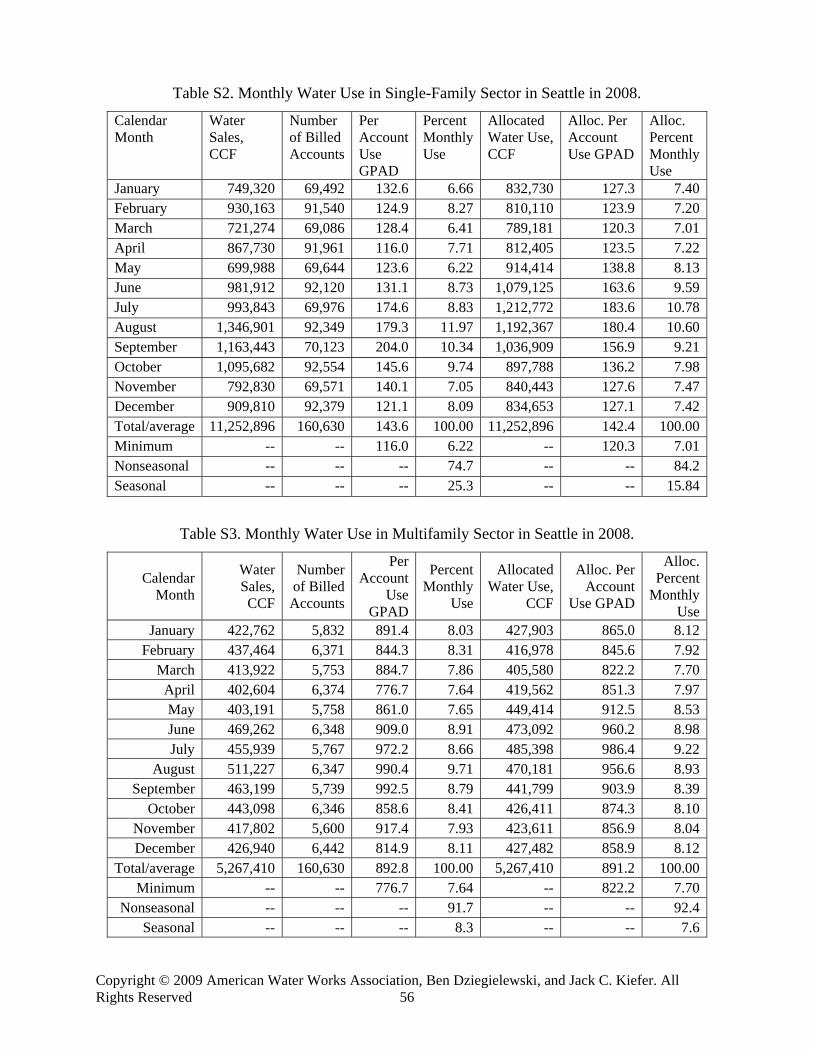
Copyright © 2009 American Water Works Association, Ben Dziegielewski, and Jack C. Kiefer. All Rights Reserved 56
Table S2. Monthly Water Use in Single-Family Sector in Seattle in 2008.
Calendar Month
Water Sales, CCF
Number of Billed Accounts
Per Account Use GPAD
Percent Monthly Use
Allocated Water Use, CCF
Alloc. Per Account Use GPAD
Alloc. Percent Monthly Use
January 749,320 69,492 132.6 6.66 832,730 127.3 7.40February 930,163 91,540 124.9 8.27 810,110 123.9 7.20March 721,274 69,086 128.4 6.41 789,181 120.3 7.01April 867,730 91,961 116.0 7.71 812,405 123.5 7.22May 699,988 69,644 123.6 6.22 914,414 138.8 8.13June 981,912 92,120 131.1 8.73 1,079,125 163.6 9.59July 993,843 69,976 174.6 8.83 1,212,772 183.6 10.78August 1,346,901 92,349 179.3 11.97 1,192,367 180.4 10.60September 1,163,443 70,123 204.0 10.34 1,036,909 156.9 9.21October 1,095,682 92,554 145.6 9.74 897,788 136.2 7.98November 792,830 69,571 140.1 7.05 840,443 127.6 7.47December 909,810 92,379 121.1 8.09 834,653 127.1 7.42Total/average 11,252,896 160,630 143.6 100.00 11,252,896 142.4 100.00Minimum -- -- 116.0 6.22 -- 120.3 7.01Nonseasonal -- -- -- 74.7 -- -- 84.2Seasonal -- -- -- 25.3 -- -- 15.84
Table S3. Monthly Water Use in Multifamily Sector in Seattle in 2008.
Calendar Month
Water Sales, CCF
Number of BilledAccounts
Per Account
Use GPAD
Percent Monthly
Use
Allocated Water Use,
CCF
Alloc. Per Account
Use GPAD
Alloc. Percent
Monthly Use
January 422,762 5,832 891.4 8.03 427,903 865.0 8.12February 437,464 6,371 844.3 8.31 416,978 845.6 7.92
March 413,922 5,753 884.7 7.86 405,580 822.2 7.70April 402,604 6,374 776.7 7.64 419,562 851.3 7.97May 403,191 5,758 861.0 7.65 449,414 912.5 8.53June 469,262 6,348 909.0 8.91 473,092 960.2 8.98July 455,939 5,767 972.2 8.66 485,398 986.4 9.22
August 511,227 6,347 990.4 9.71 470,181 956.6 8.93September 463,199 5,739 992.5 8.79 441,799 903.9 8.39
October 443,098 6,346 858.6 8.41 426,411 874.3 8.10November 417,802 5,600 917.4 7.93 423,611 856.9 8.04December 426,940 6,442 814.9 8.11 427,482 858.9 8.12
Total/average 5,267,410 160,630 892.8 100.00 5,267,410 891.2 100.00Minimum -- -- 776.7 7.64 -- 822.2 7.70
Nonseasonal -- -- -- 91.7 -- -- 92.4Seasonal -- -- -- 8.3 -- -- 7.6

Copyright © 2009 American Water Works Association, Ben Dziegielewski, and Jack C. Kiefer. All Rights Reserved 57
Table S4. Monthly Water Use in Nonresidential Sector in Seattle in 2008.
Calendar Month
Water Sales, CCF
Number of BilledAccounts
Per Account
Use GPAD
Percent Monthly
Use
Allocated Water Use,
CCF
Alloc. Per Account
Use GPAD
Alloc. Percent
Monthly Use
January 822,779 8,010 1,263.1 7.48 827,880 1,187.6 7.53February 848,759 9,244 1,129.0 7.71 803,156 1,158.2 7.30
March 791,221 7,784 1,249.9 7.19 790,461 1,138.5 7.19April 781,421 9,293 1,034.0 7.10 839,888 1,211.0 7.63May 807,779 7,775 1,277.5 7.34 938,533 1,350.7 8.53June 962,574 9,267 1,277.3 8.75 1,066,554 1,529.7 9.69July 1,021,206 7,853 1,599.0 9.28 1,163,065 1,668.8 10.57
August 1,261,229 9,311 1,665.6 11.46 1,112,770 1,599.4 10.11September 1,108,596 7,802 1,747.2 10.08 970,701 1,407.9 8.82
October 972,658 9,298 1,286.3 8.84 856,194 1,249.8 7.78November 828,893 7,464 1,365.6 7.53 810,085 1,157.6 7.36December 794,333 9,483 1,030.0 7.22 822,163 1,164.0 7.47
Total/average 11,001,448 13,461 1,674.9 100.00 11,001,448 1,318.6 100.00Minimum 781,421 1,030.0 7.10 -- 1,138.5 7.19
Nonseasonal 85.2 -- -- 86.2Seasonal 14.8 -- -- 13.8
Table S5. Historical Water Use in Single-Family and Multifamily Sectors in Seattle
Single-Family Sector Multifamily Sector Year Water Sales,
CCF Billed
Accounts Use per
Account, GPAD
Water Sales, CCF
Billed Accounts
Use per Account, GPAD
1994 13,834,558 144,989 195.5 6,954,628 118,307 120.51995 13,505,753 145,307 190.5 6,992,254 120,023 119.41996 13,111,222 145,476 184.7 7,020,046 121,739 118.21997 12,796,245 146,070 179.5 7,023,046 123,455 116.61998 13,463,537 146,586 188.2 7,114,778 125,172 116.51999 12,700,811 147,176 176.8 7,026,526 126,888 113.52000 13,171,348 147,849 182.6 7,091,105 128,604 113.02001 11,728,965 148,476 161.9 6,661,524 130,885 104.32002 12,103,025 149,131 166.3 6,386,505 133,165 98.32003 12,148,677 149,786 166.2 6,240,051 133,662 95.72004 11,827,349 150,524 161.0 6,126,420 135,671 92.52005 11,040,749 151,403 149.4 5,949,379 136,281 89.52006 11,517,353 152,623 154.6 5,996,091 138,306 88.82007 11,070,245 153,620 147.7 5,868,082 140,331 85.72008 10,733,747 155,581 141.4 5,786,559 144,930 81.8
Trend -1.69 0.48 -2.16 -1.61 1.36 -2.95

Copyright © 2009 American Water Works Association, Ben Dziegielewski, and Jack C. Kiefer. All Rights Reserved 58
CASE #6 PHILADELPHIA, PENNSYLVANIA
Table L1. System-wide Production, Consumption and Losses in Philadelphia in 2008
No. Description Calculations MGD Water supply:
1 System input 258.302 Correction for master meter and data handling error 7.593 Corrected system input (1)-(2) 250.704 Minus exports 19.405 Water supplied (city only) (3)-(4) 231.306 Authorized consumption: 7 Billed metered 162.40
10 Unbilled unmetered 2.0911 Registered authorized consumption sub-total (7)+(10) 164.4912 Customer billing over-statement adjustment -6.0213 Authorized consumption total (11)+(12) 158.49
Apparent losses: 14 Customer meter inaccuracies 0.5215 Unauthorized consumption 5.7016 Systematic data handling error 12.7717 Total apparent losses (14)+(15)+(16) 18.99
Real losses 18 Reported & unreported leakage** 19 Transmission main leaks/breaks 1.0020 Distribution main leaks/breaks 1.7621 Customer service lines 18.4922 Hydrant & valve leaks 1.6023 Measured leakage 1.9224 Background leakage 29.0525 Total real losses Σ (19)…(24) 53.8226 Total water losses (25)+(17) 72.82
Unavoidable annual real losses: 27 Total pipeline mileage (miles) 3,207 28 Average pressure (psi) 55 29 Unit pipeline losses (gal./mile/day/psi) 5.4 30 Unavoidable pipeline losses (mgd) (27)*(28)*(29) 0.9531 Number of service connections 547,932 32 Unit connection losses (gal./service/day/psi 0.15 33 Unavoidable connection losses (mgd) (28)*(31)*(32) 4.5234 Service line per connection (feet) 12 35 Unit service line losses (gal./mile/day/psi) 7.5 36 Unavoidable service line losses (mgd) (28)*(34)*(35) 0.5137 Total unavoidable real losses (mgd) (30)+(33)+(36) 5.9938 Nonrevenue water (%) (26)*100/(5) 32.439 Real resource losses (%) (25)+100/(5) 23.340 Infrastructure leakage index (25)/(37) 9.0

Copyright © 2009 American Water Works Association, Ben Dziegielewski, and Jack C. Kiefer. All Rights Reserved 59
Table L2. Historical Production, Consumption and Water Losses in Philadelphia
Description 2000 2001 2002 2003 2004 2005 2006 2007 2008 C.V. 2000-
08 Trend
Service area population (1000) 1,671.6 1,653.3 1,640.8 1,629.4 1,622.7 1,653.3 1,656.2 1,642.6 1,660.5 0.9 -0.02Water supplied from rivers, mgd 308.7 294.3 286.5 294.3 286.0 283.0 276.9 278.7 273.6 3.8 -1.26Water system input, mgd 277.7 267.5 263.0 270.2 263.0 260.3 253.8 255.3 250.7 3.3 -1.09Per capita water supplied, gpcd 184.7 178.0 174.6 180.6 176.2 171.2 167.2 169.7 164.8 3.7 -1.23Billed consumption, mgd 185.8 181.7 178.2 183.4 176.9 176.9 177.0 169.5 175.8 2.7 -0.80Unbilled unmetered, mgd 3.0 2.3 2.4 3.1 2.4 2.3 2.4 2.3 2.1 13.7 -2.93Authorized consumption, mgd 188.8 184.0 180.6 186.4 179.3 179.2 179.4 171.8 177.9 2.8 -0.82Per capita water consumed, gpcd 111.2 109.9 108.6 112.6 109.0 107.0 106.9 103.2 105.9 2.6 -0.77Apparent losses, mgd 18.6 14.5 13.1 13.3 11.1 14.1 15.1 21.8 19.0 22.0 3.06Real losses (leakage), mgd 70.1 68.9 69.2 70.5 72.6 66.9 59.2 61.6 53.8 9.5 -2.78Non-revenue water, mgd 91.8 85.7 84.7 86.9 86.1 83.3 76.7 85.7 74.9 6.2 -1.72Non-revenue water, % 33.1 32.1 32.2 32.1 35.4 34.6 32.2 36.3 32.4 4.9 0.62Unavoidable real losses (mgd) 5.7 5.4 5.3 5.9 6.0 6.1 6.7 6.0 6.0 6.8 0.73Infrastructure Leakage Index (ILI) 12.3 12.7 13.1 11.9 12.1 11.0 8.9 10.3 8.9 14.0 -4.41
Apparent losses include billing data error, unauthorized consumption, and customer metering inaccuracies. Non-revenue water volume = unbilled, unmetered consumption + apparent loss + real loss.

Copyright © 2009 American Water Works Association, Ben Dziegielewski, and Jack C. Kiefer. All Rights Reserved 60
CASE #7 TAMPA WATER DEPARTMENT, FLORIDA
Table T1. Annual Production, Sales and Billed Accounts Data for Tampa Water Department, Florida
Description 2004 2005 2006 2007 2008 C.V. Trend %/year
Population served 605,073 655,993 647,131 656,837 657,313 3.5 1.65Production (mgd) 28,721.8 26,924.8 27,725.5
029,761.7 27,725.5 3.9
-1.46Total metered sales (mgd): 24,034.4 23,882.2 25,161.62 25,745.0 25,123.7 4.0 2.54 Total residential 14,867.9 15,462.4 16,386.02 15,982.1 15,666.3 3.7 1.43 Single-family res. 9,700.1 10,502.6 10,908.35 10,550.7 10,317.7 4.3 1.34 Multifamily res. 5,167.8 4,959.8 5,477.68 5,431.4 5,348.6 4.1 1.6 Commercial 5,357.6 5,491.0 5,522.23 5,444.2 5,334.9 1.4 -0.21 Industrial 1,416.6 1,181.3 1,328.57 1,312.6 1,190.6 7.8 -2.16 Governmental 282.5 3.7 3.01 131.4 57.1 122.4 -- Public Mixed nonresidential 1,257.03 Wholesale deliveries 439.3 664.76 1,439.4 1,439.4 42.0 52.78No. of billed accounts: 122,340 123,801 125,887 126,089 125,139 1.3 0.82 Total residential 109,612 111,105 112,886 113,455 112,257 1.4 0.69 Single-family res. 107,717 109,167 110,912 111,445 110,140 1.3 0.65 Multifamily res. 1,895 1,938 1,974 2,010 1,997 2.4 3.09 Commercial 11,936 11,926 11,969 12,056 11,956 0.4 0.14 Industrial 204 201 203 201 213 2.4 0.88 Governmental 11 12 257 18 252 120.0 -- Public 227 226 226 225 223 0.7 -0.4 Combined nonresidential 337 332 333 346 345 1.9 0.89 Wholesale deliveries 13 13 13 13 13 0.0 0

Copyright © 2009 American Water Works Association, Ben Dziegielewski, and Jack C. Kiefer. All Rights Reserved 61
Table T2. Calculated Metrics Using the Number of Accounts and Population Served as Normalizing Variables
Description 2004 2005 2006 2007 2008 C.V. Trend %/year
Per account metrics (gpad): Total residential 372 381 398 386 382 2.5 0.69 Single-family 247 264 269 259.4 256.7 3.3 0.63 Multifamily 7,471 7,012 7,602 7,403 7,338 3.0 -1.38 Commercial 1,230 1,261 1,264 1,237 1,223 1.4 -0.35 Industrial 19,025 16,102 17,931 17,892 15,315 8.8 -2.99 Governmental 70,361 845 32 19,993 621 164.8 -- Mixed nonresidential -- -- 0 -- -- -- -- Total nonresidential 213 1,005 10,342 482 1,051 50.4 0.79 Wholesale deliveries 92,582 140,096 303,345 303,345 42.0 52.78 Al sales/all accounts 538 529 548 559 550 2.9 2.6Per capita metrics (in gpcd): Pr capita production 130.1 112.5 117.4 124.1 115.6 5.9 -3.25 Total sales per capita 108.8 99.7 106.5 104.1 110.8 4.5 0.8 Residential sales per capita 67.3 64.6 69.4 66.2 65.7 1.5 -0.24 Nonresidential sales per capita 32 33.3 34.3 34.2 33.4 2.4 1.12Nonrevenue water (%) 16.3 11.3 9.3 15.8 9.4 84.3 -61.44
Table T3. Monthly and Seasonal Single-Family Residential Usage Rates in Tampa, Florida.
Month 2004 2005 2006 2007 2008Per account use (gpad): January 221.2 290.0 271.4 275.9 264.5February 329.3 277.9 257.3 250.7 319.4March 289.2 264.2 233.0 226.6 240.4April 322.2 272.7 256.3 247.8 237.0May 239.7 264.2 325.0 249.1 212.5June 228.9 265.0 320.1 294.5 266.3July 194.1 272.0 316.2 289.5 291.1August 235.4 234.9 234.0 303.8 315.5September 240.4 257.9 247.7 241.1 225.6October 194.2 238.7 223.3 225.3 220.8November 235.2 278.6 275.9 243.9 238.7December 240.4 249.2 272.6 244.9 273.1Annual average 246.7 263.6 269.4 257.8 258.4Minimum month 194.1 234.9 223.3 225.3 212.5Percent nonseasonal 80.2 91.0 82.9 89.2 84.0Percent seasonal 19.8 9.0 17.1 10.8 16.0

Copyright © 2009 American Water Works Association, Ben Dziegielewski, and Jack C. Kiefer. All Rights Reserved 62
Table T4. Monthly and Seasonal Multifamily Residential Usage Rates in Tampa, Florida.
Month 2004 2005 2006 2007 2008Per account use (gpad): January 6,833 8,340 7,950 8,074 7,940February 8,833 8,263 7,534 7,494 7,878March 7,478 7,509 6,874 7,034 6,928April 8,255 7,787 6,942 7,251 6,849May 7,305 7,534 7,808 7,876 7,062June 7,763 7,554 8,065 7,759 7,754July 6,735 7,935 8,430 7,222 7,573August 7,650 7,423 7,199 6,764 6,856September 7,393 7,715 7,629 7,583 7,235October 6,675 6,732 6,830 6,666 7,306November 7,691 8,064 8,230 7,340 7,524December 7,263 7,423 7,784 7,840 7,203Annual average 7,472 7,012 7,606 7,409 7,342Minimum month 6,675 6,732 6,830 6,666 6,849Percent nonseasonal 91.4 94.3 89.8 90.0 93.3Percent seasonal 8.6 5.7 10.2 10.0 6.7
Table T5. Monthly and Seasonal Nonresidential Usage Rates in Tampa, Florida.
Month 2004 2005 2006 2007 2008Per account use (gpad): January 2,007 1,816 1,496 2,806 1,417February 2,365 1,839 1,640 1,596 1,495March 2,084 1,658 1,398 1,277 1,260April 2,114 1,748 1,593 1,569 1,432May 2,034 1,782 1,634 1,518 1,368June 1,816 1,824 1,812 1,705 1,579July 1,873 1,831 1,676 1,486 1,414August 1,783 1,676 1,544 1,588 1,380September 1,985 1,572 1,543 1,436 1,295October 1,385 1,725 1,578 1,375 1,456November 1,565 1,821 1,724 1,404 1,277December 1,711 7,423 1,739 1,620 1,374Annual average 1,894 1,722 1,615 1,615 1,396Minimum month 1,385 1,572 1,398 1,277 1,260Percent nonseasonal 73.1 69.9 86.6 79.1 90.3Percent seasonal 26.9 30.1 13.4 20.9 9.7