avoiding invalid instruments and coping with weak instruments - smu

American Economic Association

Avoiding Invalid Instruments and Coping with Weak InstrumentsAuthor(s): Michael P. MurraySource: The Journal of Economic Perspectives, Vol. 20, No. 4 (Fall, 2006), pp. 111-132Published by: American Economic AssociationStable URL: http://www.jstor.org/stable/30033686Accessed: 28/04/2010 11:40

Your use of the JSTOR archive indicates your acceptance of JSTOR's Terms and Conditions of Use, available athttp://www.jstor.org/page/info/about/policies/terms.jsp. JSTOR's Terms and Conditions of Use provides, in part, that unlessyou have obtained prior permission, you may not download an entire issue of a journal or multiple copies of articles, and youmay use content in the JSTOR archive only for your personal, non-commercial use.

Please contact the publisher regarding any further use of this work. Publisher contact information may be obtained athttp://www.jstor.org/action/showPublisher?publisherCode=aea.

Each copy of any part of a JSTOR transmission must contain the same copyright notice that appears on the screen or printedpage of such transmission.

JSTOR is a not-for-profit service that helps scholars, researchers, and students discover, use, and build upon a wide range ofcontent in a trusted digital archive. We use information technology and tools to increase productivity and facilitate new formsof scholarship. For more information about JSTOR, please contact [email protected].

American Economic Association is collaborating with JSTOR to digitize, preserve and extend access to TheJournal of Economic Perspectives.

http://www.jstor.org

http://www.jstor.org/stable/30033686?origin=JSTOR-pdf

http://www.jstor.org/page/info/about/policies/terms.jsp

http://www.jstor.org/action/showPublisher?publisherCode=aea

Journal of Economic Perspectives-Volume 20, Number 4-Fall 2006-Pages 111-132

Avoiding Invalid Instruments and Coping with Weak Instruments

Michael P. Murray

Archimedes

Archimedes said, "Give me the place to stand, and a lever long enough, and I will move the Earth" (Hirsch, Kett, and Trefil, 2002, p. 476). Economists have their own powerful lever: the instrumental variable estimator. The

instrumental variable estimator can avoid the bias that ordinary least squares suffers when an explanatory variable in a regression is correlated with the regression's disturbance term. But, like Archimedes' lever, instrumental variable estimation

requires both a valid instrument on which to stand and an instrument that isn't too short (or "too weak"). This paper briefly reviews instrumental variable estimation, discusses classic strategies for avoiding invalid instruments (instruments themselves correlated with the regression's disturbances), and describes recently developed strategies for coping with weak instruments (instruments only weakly correlated with the offending explanator).

As an example of biased ordinary least squares, consider whether incarcerating more criminals reduces crime. To estimate the effect of increased incarceration on

crime, an economist might specify a regression with the crime rate as the dependent variable and the incarceration rate as an explanatory variable. In this regression, the naive ordinary least squares regression could misleadingly indicate that high rates of incarceration are causing high rates of crime if the actual pattern is that more crime leads to more incarceration. Ordinary least squares provides a biased estimate of the effect of incarceration rates on crime rates in this case because the incarceration rate is correlated with the regression's disturbance term.

As another example, consider estimating consumption's elasticity of intertemporal substitution (which measures the responsiveness of consumption patterns to changes in intertemporal prices). To estimate this elasticity, economists typically specify a linear relationship between the rate of growth in consumption and the

SMichael P. Murray is the Charles Franklin Phillips Professor of Economics, Bates College, Lewiston, Maine. His e-mail address is ([email protected]).

112 Journal of Economic Perspectives

expected real rate of return, with a coefficient on the expected real rate of return that equals the elasticity of intertemporal substitution. Unfortunately, the expected real rate of return is not generally observed, so in empirical practice economists instead use the actual rate of return, which measures the expected rate of return with error. Using a mismeasured explanator biases ordinary least squares-the effect of the measurement error in the explanator ends up being "netted out" in the disturbance term, so the mismeasured explanator is negatively correlated with the disturbance term.

In both examples, ordinary least squares estimation is biased because an

explanatory variable in the regression is correlated with the error term in the

regression. Such a correlation can result from an endogenous explanator, a mismeasured explanator, an omitted explanator, or a lagged dependent variable

among the explanators. I call all such explanators "troublesome." Instrumental variable estimation can consistently estimate coefficients when ordinary least

squares cannot-that is, the instrumental variable estimate of the coefficient will almost certainly be very close to the coefficient's true value if the sample is

sufficiently large--despite troublesome explanators.' Regressions requiring instrumental variable estimation often have a single

troublesome explanator, plus several nontroublesome explanators. For example, consider the regression

I,

in which Yli

is the dependent variable of interest (for example, the crime rate), Y2i is the troublesome explanator (for example, the incarceration rate), and Xi is a vector of nontroublesome explanators (for example, the proportion of the population aged 18-25).

Instrumental variables estimation is made possible by a set of variables, Z, that are 1) uncorrelated with the error term ei, 2) correlated with the troublesome

explanator Y2i, and 3) not explanators in the original equation. The elements of Z are called instrumental variables. In effect, instrumental variable estimators use the elements of Zand their correlation with the troublesome explanator to estimate the coefficients of an equation consistently.

The most frequently used instrumental variable estimator is two-stage least

squares. For simplicity, consider the case with just one troublesome explanatory variable. In this case, the first stage in two-stage least squares regresses the troublesome explanator (for example, the incarceration rate) on both the instrumental variables that make up the elements of Z and the nontroublesome explanators, X,

SFor modern introductory treatments of instrumental variable estimation, see Murray (2006, chap. 13) and Stock and Watson (2003, chap. 10). A much longer variant of this paper uses seven empirical papers to illustrate both nine strategies for checking an instrument's validity and a class of new test procedures that are robust to weak instruments (Murray, 2005). For articles that cite many recent instrumental variable analyses, see Angrist and Krueger (2001) in this journal and Murray (2005).

Michael P. Murray 113

using ordinary least squares. This first-stage regression (often called a "reduced form equation") is:

Y2i = Oo

+ Zi4Y1 + 2 + i.

The researcher then uses the ordinary least squares coefficient estimates from this first-stage regression to form fitted values, 2i, for the troublesome variable. For example, the Y2i might be the fitted values for the incarceration rate in a study of crime rates. In the second stage of two-stage least squares, these fitted values for the troublesome explanator are substituted for the actual values of the troublesome variable in an ordinary least squares regression of Yi on Xand Y2i (for example, the crime rate is regressed on X and on the fitted value of the incarceration rate, using ordinary least squares). The second-stage coefficient estimates are the two-stage least squares estimates.

Two-stage least squares requires at least as many instruments as there are troublesome explanators. When there are too few instruments, we say the equation of interest is under-identified. When the number of instruments equals the number of troublesome variables, we say the equation of interest is exactly identified. When the number of instruments exceeds the number of troublesome explanators, we say the equation is over-identified. Strictly speaking, having at least as many instruments as troublesome variables is only a necessary condition for identification. In most applications, the condition proves sufficient. However, when there are multiple troublesome variables, some additional attention should be given to ensuring identification.2

The two-stage least squares estimator has larger standard errors than does ordinary least squares. Consequently, guarding against or overcoming the possible biases of ordinary least squares by using instrumental variables always comes at a cost. The loss of efficiency results because two-stage least squares uses only that part of the variation in the troublesome explanator, Y2, that appears as variation in the fitted values, the elements of iY2.

Exact identification requires that the number of variables included in Z, and thus excluded from X, be equal to the number of troublesome variables. Excluding a variable from X is, therefore, sometimes called an "identifying restriction." When an equation is over-identified, we speak of corresponding "over-identifying restrictions." An increased number of over-identifying restrictions generally confers the benefit of a higher 1R2 in the first stage of two-stage least squares and, therefore, yields standard errors closer to those of ordinary least squares.

Instrumental variable estimation can cure so many ills that economists might

2 The requirement that the instrumental variables are not explanators in the original equation echoes the classic simultaneous equation "order condition" for identification: to be identified, an equation must exclude at least one exogenous variable for each endogenous explanator it contains-the excluded exogenous variables are then available for inclusion in Z. While the order condition is necessary for identification, it is the "rank condition" that suffices for identification. See Murray (2006, pp. 617-618) for an intuitive discussion of the rank condition.


be tempted to think of it as a panacea. But a prospective instrument can be flawed in either of two debilitating ways. First, an instrument can itself be correlated with the disturbance term in the equation of interest. We call such instruments "invalid." Invalid instruments yield a biased and inconsistent instrumental variable estimator that can be even more biased than the corresponding ordinary least squares estimator. Indeed, all instruments arrive on the scene with a dark cloud of invalidity hanging overhead. This cloud never goes entirely away, but researchers should chase away as much of the cloud as they can. Second, an instrument can be so

weakly correlated with the troublesome variable that in practice it will not overcome the bias of ordinary least squares and will yield misleading estimates of statistical

significance even with a very large sample size. We call such instruments "weak." Researchers need to guard against drawing misleading inferences from weak instruments.

How can economists determine that a prospective instrumental variable is valid? Must the correlation between a potential instrument and the error term be

exactly zero? And how can economists determine when an instrumental variable is too weak to be useful? This article uses works by Steven Levitt (1996, 1997, 2002) that assess policies to reduce crime and Motohiro Yogo's 2004 work that estimates

consumption's elasticity of intertemporal substitution, to illustrate the recent an- swers of econometricians to these fundamental questions. Levitt gives particular care to assessing his instruments' validity, while Yogo exploits recent theoretical advances to grapple with weak instruments.

Supporting an Instrument's Validity

Levitt (1996) analyzes the effect of changes in incarceration rates on changes in crime rates with instruments rooted in prison-overcrowding lawsuits that took

place in a dozen states across a span of 30 years. These dozen states were sometimes involved in such suits and sometimes not. Other states were never involved in such

lawsuits. Levitt expected (and found) that overcrowding litigation and incarceration rate changes are negatively correlated-when such suits are filed, states de-

fensively work to reduce incarceration rates, and when such suits are won by plaintiffs, there are further declines in prison populations. Levitt bases his instruments on the stages of prison overcrowding lawsuits from filing through judgment. He argues (p. 323) that his litigation status instruments are valid because "it is

plausible that prison overcrowding litigation will be related to crime rates only through crime's impact on prison populations, making the exclusion of litigation status itself from the crime equation valid."

Instrumental variable estimation can sometimes expose substantial biases in

ordinary least squares. Using two-stage least squares, Levitt (1996) estimates that the effects of incarceration in reducing crime are two or three times larger in

magnitude than indicated by previous ordinary least squares estimates. He estimates that the marginal benefit from incarcerating one prisoner for an additional

year is $50,000. Published estimates of the costs of incarceration indicate that one

Avoiding Invalid Instruments and Coping with Weak Instruments 115

year costs the state about $30,000. Levitt (p. 324) concludes that "the current level of imprisonment is roughly efficient, though there may be some benefit from lengthening the time served by the current prisoner population."

Levitt (1997, 2002) has also analyzed the effects of police officers on crime. Because the number of police officers a community hires is influenced by the

community's crime rate, ordinary least squares is biased when applied to a regression in which the dependent variable is the crime rate and one explanator is the number of police officers per 100,000 population. In his papers studying the effects of police on crime, Levitt offers two instrumental variable strategies for consistently estimating the effects of police on crime.

In his earlier police paper, Levitt (1997) proposes mayoral and gubernatorial election cycles as instruments for changes in the number of police officers, on the

empirically supported supposition that changes in the number of officers would be correlated with mayors and governors running for re-election. (Mayors and governors running for office have an incentive to increase the quality of public services, including police protection, in the period shortly preceding elections.) Levitt's use of mayoral and gubernatorial election cycles falls prey to the efficiency loss that

always accompanies instrumental variables estimation. Using those instruments, the standard errors of Levitt's instrumental variable estimates are ten times the size of

the standard errors from the corresponding ordinary least squares estimation. Levitt's data yield a large instrumental variable estimate of the effect of police on violent crime rates, but the estimated effect is not significantly different from zero because the standard errors are so large. The lesson here is that even valid instruments that are correlated with the troublesome variable might still prove too inefficient to be informative.

Levitt's second instrumental variable strategy for examining the effect of police proves somewhat more informative. When McCrary (2002) showed that a program- ming error in Levitt's (1997) computations led to an instrumental variable estimate of the effect of police on violent crime that was too large and erroneously significant, Levitt (2002) took the opportunity to reassess the effect of police on crime rates by using the number of firefighters in a city as an instrument for the number of police. The intuitive argument here is that some of the variation in hiring police officers is due to the general state of municipal budgets, which should also show up in hiring of firefighters. The firefighter instrument yields a substantial negative estimated effect of police on crime. The estimate is smaller than the coefficient using election cycles, but it is also more precisely estimated, so the estimated effect of police on crime attains marginal statistical significance.

How much credence should be granted to instrumental variable analyses like Levitt's? It depends in part on the quality of the arguments made for the instruments' validity. In his crime papers, Levitt tests over-identifying restrictions, counters anticipated arguments about why his instruments are invalid, takes particular care with what variables are omitted from his model, compares results from alternative instruments, and appeals to intuitions that suggest his instruments' validity. The kinds of arguments Levitt makes to support the validity of his instruments are not unique to him, nor do they exhaust the ways we can support the


validity of instruments,3 but Levitt does marshal an unusually varied array of

arguments in support of his instruments' validity. His strategies warrant review.

Test Over-identifying Restrictions Valid instruments cannot themselves be relevant explanators. How, then, are

we to determine that a candidate instrument is not a relevant explanator? Can we

formally test whether a lone candidate instrument can be legitimately excluded from the equation of interest? For example, can we just add the candidate instrument to the model as a potential explanator and use ordinary least squares to test whether the candidate instrument is actually itself an explanator in the equation? No, this approach will not work because the equation's troublesome variable biases the ordinary least squares estimator used for such a test. However, over-identified

equations do allow a variant of this test. When examining the effect of incarceration rates on crime and in the appli-

cation of his first instrumental variable strategy for studying the effect of police on crime, Levitt's crime rate equations are over-identified. In the former case, his instruments capture the status of prison overcrowding lawsuits in a state (such as

filing and preliminary decision) and also distinguish between status in the year of an observation and status in years preceding an observation. In all, this yields ten lawsuit status variables to use as instrumental variables for the one troublesome

variable. In the latter case, Levitt has two basic instruments-the gubernatorial and

mayoral cycle variables-for his one troublesome variable; he further increases the number of instruments by interacting the election-cycle variables with city-size or

region dummies. Each additional over-identifying restriction is attractive in that it can lessen the

rise in standard errors that accompanies moving from ordinary least squares to

two-stage least squares. We can also exploit such over-identification to test the

validity of some instruments. Intuitively, if Levitt knew that he had enough surely valid instruments to exactly identify his crime equation, he could use those instruments alone to carry out a consistent two-stage least squares estimation in which the

remaining potential instruments were included among the explanators (that is, in

X), rather than being used as instruments (that is, in Z). Failing to reject the null

hypothesis that these remaining potential instruments all have zero coefficients in the second stage of two-stage least squares when included in X as explanators would support the validity of those extra variables as instruments. The key to this strategy's success is knowing for sure that an exactly identifying subset of the instruments are indeed valid so that two-stage least squares estimation is both

possible and consistent. However, most researchers don't know that some of their instruments are

surely valid. Nor did Levitt. Instead, Levitt used a test of over-identifying restrictions

3 Murray (2005) uses seven empirical papers to illustrate nine strategies for supporting instruments' validity.


devised by Sargan (1958), which is available in some regression packages4 and does not require the researcher to indicate in advance which instruments are valid and which doubtful. Sargan's test asks whether any of the instruments are invalid, but assumes, as in the intuitive two-stage least squares over-identification test, that at least enough are valid to identify the equation exactly. If too few of the instruments are valid, Sargan's test is biased and inconsistent.

In the incarceration study, Levitt fails to reject the null hypothesis that all of his instruments are valid. In the police study using election-cycle instruments, Levitt obtains mixed results when testing the validity of all of his instruments; in some specifications, the test is passed, in others it is failed. On this ground, Levitt's instrumental variable estimate of the effect of incarceration rates on crime rates is more credible than his estimates of the effects of police officers on crime rates.

What is the chance that Sargan's test is invalid in Levitt's applications? In Levitt's (1997) crime study, all of the instruments are grounded in political cycles; in Levitt's (1996) study, all the instruments are grounded in overcrowding lawsuits. Sargan's test is suspect when all the instruments share a common rationale-if one instrument is invalid, it casts doubt on them all. For example, if we knew for certain that one lawsuit-related instrument was invalid, we would be apt to worry that they all were-and therefore that Sargan's test is invalid. In contrast, if Levitt could combine firefighters and election cycles as instruments in a single analysis, a failure to reject the over-identifying restrictions in such a model would have provided more comfort about the instruments' likely validity since these instrumental variables are grounded in different rationales-one might be valid when the other is not. Unfortunately, many of the cities used with the firefighter instrumental variable strategy do not have mayoral governments, so Levitt isn't able to combine these two instrumental variable strategies for estimating the effects of police on crime rates into a single approach.

Some economists are very wary of over-identification tests, because they rest on there being enough valid instruments to over-identify the relationship. Their worry is that too often, a failure to reject the null hypothesis of valid over-identifying restrictions tempts us to think we have verified the validity of all of the instruments. Economists should resist that temptation.

Preclude Links between the Instruments and the Disturbances In his study of incarceration rates, Levitt (1996) attempts to anticipate and test

possible arguments about why his lawsuit instruments might be invalid. For example, one potential criticism is that prison overcrowding lawsuits might result from

4 Sargan's test statistic is nR2 using the R2 from a regression of residuals from the equation of interest (fit using the two-stage least squares estimates of that equation's parameters) on the elements of Z. The statistic has a chi-square distribution with degrees of freedom equal to (1 - q), the degree of over- identification. The Stata command ivreg2 yields Sargan's test statistic. This command is an add-on to Stata. To locate the ivreg2 code from within Stata, type "findit ivreg2" on Stata's command line. Then click on the website name given for ivreg2 to update Stata. There are other tests for over-identifying restrictions. In EViews, the generalized method of moments (GMM) procedure reports Hansen'sJ-test, which is a more general version of Sargan's test.


past swells in crime rates even if incarceration rates were unchanged. If this were so, and if such shocks to crime rates tended to persist over time, then the instrument would be invalid. Levitt tackles the possibility head-on. He investigates whether

over-crowding lawsuits can be predicted from past crime rates, and finds they cannot.

In his second study of police officers' effect on crime rates, Levitt (2002) anticipates two arguments that challenge the validity of the firefighter instrument. First, city budget constraints might mean that increases in crime rates that spur hiring more police officers lead to fewer firefighters (and lower other expenditures). Second, some increases in crime rates that spur adding police officers might also increase the need for firefighters (for example, a larger low-income population could be associated with both higher crime rates and more fire-prone residences). Unfortunately, Levitt offers no strategy for empirically assessing these specific arguments against the firefighter instrument's validity, and, as a result, Levitt's

firefighter results are less compelling than they might otherwise be.

Be Diligent About Omitted Explanators Every ordinary least squares analysis must be concerned about omitting ex-

planatory variables that belong in the model. Ordinary least squares estimation is biased if such omitted variables are correlated with the included explanators. When

doing instrumental variable estimation, this concern arises in a new form. Instru- mental variable estimation is biased if an omitted explanator that belongs in the model is correlated with either the included nontroublesome explanators (the X

variables) or the instrumental variables (the Zvariables). This concern requires that researchers be doubly vigilant about omitted variables when doing instrumental variable estimation.

In his first police study, Levitt's (1996) instrument is mayoral and gubernatorial election cycles. He is careful to include local welfare expenditures among his

explanators, because these might lower crime rates and because they are plausibly correlated with election cycles. Even if the correlation between welfare expenditures and numbers of police officers were zero (so that omitting welfare expenditures as an explanator would not bias ordinary least squares), welfare expenditures' correlation with mayoral and gubernatorial election cycles might be large, in which case omitting such a variable could seriously bias the instrumental variable estimate of the effect of police officers on crime rates. In his second police study, using the

firefighter instrument, Levitt (2002) adds a string of city-specific explanatory variables to his crime rate model to reduce the chance that the number of firefighters is correlated with omitted relevant variables. In both studies, Levitt uses his panel data to estimate fixed effects models or models in first differences to further reduce

the peril that omitted relevant variables might bias his instrumental variable results.

Use Alternative Instruments

Getting similar results from alternative instruments enhances the credibility of instrumental variable estimates. For example, Levitt (2002) suggests that there is some comfort to be taken from the fact that his point estimates of the effect of


police on crime using either political cycles or firefighter hiring both yield negative coefficients of appreciable magnitude. The point is a fair one, though it would be more comforting still if both estimates were statistically significant.

Sargan's formal over-identification test is, in essence, grounded in this same query: Do all of the instruments tell the same story about the parameters of interest? When it is not feasible to conduct formal over-identification tests by including all instruments in a single instrumental variable estimation, there is still information to be had by comparing the results from applying several instruments separately from one another. If the parameter estimates using different instruments differ appreciably and seemingly significantly from one another, the validity of the instruments becomes suspect. If all of the estimates are consonant with a single interpretation of the data, their credibility is enhanced.

Use and Check Intuition

Levitt (2002, p. 1245) makes a simple argument for the validity of the firefighter instrument: "There is little reason to think that the number of firefighters has a direct impact on crime." An intuitive argument for why an instrument is valid is better than no argument at all. Levitt goes to great lengths to provide arguments besides intuition for the validity of his instruments, but intuition is one more tool in his kit.

Of course, intuition need not stand naked and alone. Intuition can be checked. One useful check is to run reduced form regressions with the instrumental variable as the explanatory variable, and either the dependent variable of interest or the troublesome explanator as the dependent variables. For example, Levitt (1996) considers regressions with the prison-overcrowding litigation instruments as explanators for his dependent variable (changes in crime rates). Levitt finds that in this regression, the instrumental variables all have coefficients that are significantly different from zero with signs that support his identification story: increases in crime rates follow litigation, especially successful litigation. Further- more, Levitt finds that the litigation variables for the period just before litigation are associated with increases in prison populations, while the litigation variables for the period during the litigation and after a judgment unfavorable to the state are associated with declines in prison populations, as his identification story would suggest.

When using these reduced form regressions to check the intuition behind an instrumental variable, it would be a danger sign to find that the coefficient on an instrumental variable has a sign that is at odds with the instrument's intuition.

Pretesting variables in regression analysis has long been known to lead to inconsistency (Leamer, 1978; Miller, 1990). Recently, Hansen, Hausman, and Newey (2005) explore pretesting in the specific case of instrumental variable estimation; they conclude that fishing in a set of potential instruments to find significant ones is also a poor idea. The set of instruments should be assessed together; Arellano, Hansen, and Sentana (1999) offer a suitable formal test. With data mining frowned upon, it is all the more important to diligently apply intuition when selecting potential instruments.


The cloud of uncertainty that hovers over instrumental variable estimates is never entirely dispelled. Even if formal tests are passed and intuition is satisfied, how much credence you grant to any one instrumental variable study can legitimately differ from how much credence I grant it. But that said, Levitt's work shows how the thorough use of validity checks can lighten the clouds of uncertain validity.

Coping with Weak Instruments

The intertemporal elasticity of substitution, which measures the responsiveness of consumption patterns to changes in intertemporal prices, plays an important role in a number of economic applications. For a broad class of preferences defined

by Epstein and Zin (1989), an investor consumes a constant fraction of wealth only if his or her elasticity of intertemporal substitution is one. (With such a unitary elasticity, if the expected real rate of return were to rise two percentage points, the ratio of tomorrow's consumption to today's consumption would rise by 2 percent.) For a commonly assumed subset of Epstein-Zin preferences, such a unitary elas-

ticity also implies that the investor is myopic (Campbell and Viciera, 2002). In many neo-Keynesian macro models, the elasticity is a parameter of an intertemporal IS curve that ties together the current interest rate, the expected future interest rate, and the equilibrium level of current output (Woodford, 2003). Motohiro Yogo (2004) estimates the intertemporal elasticity of substitution in an analysis that

exemplifies current best practice for dealing with weak instruments.

Yogo (2004) estimates the intertemporal elasticity of substitution, 4, in each of eleven countries, and tests in each country the null hypothesis that the elasticity is

equal to one. Yogo specifies that consumption growth depends on the expected real rate of return. For a utility-maximizing consumer with Epstein-Zin preferences, 4 is the slope coefficient on the expected real rate of return. In general, the

elasticity is positive because a higher expected interest rate spurs consumers to save

by shifting consumption from the present into the future. Because the expected real rate of return is not generally observed, Yogo

substitutes the actual real rate of return for the expected rate. The actual real rate of return measures the expected real rate of return with error, so ordinary least

squares estimation would be biased if Yogo used it to estimate P. To avoid this bias, Yogo uses instrumental variables estimation. His instruments are lagged values of 1) the nominal interest rate, 2) inflation, 3) the log of the dividend-price ratio, and

4) the growth in consumption. He estimates that the elasticity is less than one in all eleven of the countries he studies, and he rejects everywhere the null hypothesis of a unitary elasticity.

Yogo is not the first economist to estimate the elasticity of intertemporal substitution using lagged economic variables as instruments. For example, Hall

(1988) also regresses the growth in consumption on the real rate of return to estimate 4, and Hansen and Singleton (1983) estimate the "reverse regression," with the real rate of return as the dependent variable and the growth in

consumption as the explanator to obtain 1/P. Both of these studies performed


instrumental variable estimation with identification strategies quite similar to Yogo's. These two regression approaches have created a long-standing puzzle. Regressions of consumption growth on the real rate of return tend to yield small instrumental variable estimates of the intertemporal elasticity of substitution P, but the reverse instrumental variable regressions imply large estimates of P.

Yogo uses the latest instrumental variable techniques to resolve this puzzle and to narrow greatly the range of plausible estimates of the elasticity of intertemporal substitution. Yogo's work reveals that the puzzle of the estimated size of the intertemporal elasticity of substitution arose because researchers relied on weak instruments.

Although the primary focus here will be on the problems weak instruments

pose for two-stage least squares and how Yogo deals with those problems, his argument for the validity of these instruments deserves mention. He appeals to economic theory to establish the validity of his instruments. Rational expecta- tions and efficient market hypotheses declare that current changes in some variables-perhaps most famously the stock market-will be uncorrelated with all past outcomes. Hall (1988) applies a similar argument to consumption in the context of a consumer who decides how much to consume in a year out of his or her lifetime income. Hall (p. 340) writes: "Actual movements of consumption differ from planned movements by a completely unpredictable random variable that indexes all the information available next year that was not incorporated in the planning process the year before." Hall's argument provides a theoretical basis for Yogo's (2004) use of lagged economic variables as instruments for the real rate of return: past (that is, lagged) variables are not systematically correlated with unexpected changes in current consumption. To overcome problems raised by consumption measures being aggregated across a year (Hall, 1988), Yogo lags his instrumental variables two years, instead of one.

As a starting point to understanding the problems posed by weak instrumental variables, it is useful to review the virtues of "strong" instruments (instruments that have a high correlation with the troublesome explanator). If an equation is over-identified, so that the number of instruments exceeds the number of troublesome explanators, strong instruments can provide estimates of coefficients that have small biases and approximately normal standard errors in moderately large samples. In particular, when the researcher claims that a coefficient from a two-stage least squares regression is statistically significant at the 5 percent level, the level is actually approximately 5 percent in moderately large samples. (One additional caveat here: the number of instruments should not be large relative to the sample size.) Even in the exactly identified case, in moderately large samples the two-stage least square's median is, on average, about equal to the true parameter value5 and inferences based on two-stage least squares tend to be approximately valid.

SThe reference here is to the median rather than the mean because when an equation is exactly identified the finite-sample mean of two-stage least squares is infinite. When an equation is exactly identified, or has one over-identifying restriction, two-stage least squares' finite sample variance does not


When instruments are weak, however, two serious problems emerge for two-

stage least squares. First is a problem of bias. Even though two-stage least squares coefficient estimates are consistent--so that they almost certainly approach the true value as the sample size approaches infinity-the estimates are always biased in finite samples. When the instrumental variable is weak, this bias can be large, even in very large samples. Second, when an instrumental variable is weak, two-stage least

squares' estimated standard errors become far too small. Thus, when instruments are weak, confidence intervals computed for two-stage least squares estimates can be very misleading because their mid-point is biased and their width is too narrow, which undermines hypothesis tests based on two-stage least squares. Let's consider these two difficulties in turn.

The Finite-Sample Bias in Two-Stage Least Squares That two-stage least squares can be biased in finite samples is understood most

simply by considering the case in which the only explanator in the equation of interest is a single troublesome variable and the number of instruments equals the number of observations. In this case, the first stage of two-stage least squares fits the troublesome variable exactly-ordinary least squares always fits perfectly when the number of variables equals the number of observations. Consequently, in this case, the second stage of two-stage least squares simply replaces the troublesome variable with itself, and the two-stage least squares estimator equals the (biased) ordinary least squares estimator.

It is long-established that two-stage least squares will estimate coefficients with a bias in all finite sample sizes, as explained by Rothenberg (1983, 1984) and

Phillips (1983) in their quite general treatments of two-stage least squares' finite-

sample properties. Nelson and Startz (1990a, 1990b) offer a nicely simplified approach that highlights the finite-sample problems of two-stage least squares without losing substance. So let's simplify.

Assume that the single explanator in an ordinary least squares regression is troublesome. Thus, the original ordinary least squares regression becomes:

YVo = + P31 Y2i + e i.

Instrumental variables Z are used to derive a new value for the troublesome

explanator Y2i by using the regression:

Y2i = ao + ZC tl

+ io

For convenience, choose units of measure for Y1 and Y2 such that Var(e,) = 1 and

Var(ti) = 1. A consequence of these variance assumptions is that the Cov(i, ,si)

exist either. In these cases, two-stage least squares can be wildly wrong more often than we might anticipate.


equals the correlation coefficient of ei and pi, which we call p. Because the instruments in Z are uncorrelated with ei (by assumption), p also measures the degree to which Y2 is troublesome-that is the degree to which Y2 is correlated with the disturbances in the original ordinary least squares regression. Finally, let 12 refer to how much of the variance in the troublesome explanator, Y2, is explained in the population by the instrumental variables Z in the second equation; in other words, /2 measures the strength of the correlation between the instrumental variables and the troublesome variable.

Hahn and Hausman (2005) show that, in this simplified specification, the

finite-sample bias of two-stage least squares for the over-identified situation in which the number of instrumental variables exceeds the number of troublesome variables

is, to a second-order approximation:

lp(1 - A2) E(I3SLS)

- 31 n2

This equation requires some unpacking. The left-hand side expresses the bias of the two-stage least squares coefficient-it is the expected value of the two-stage least squares estimator of the coefficient of interest minus the true value of that coefficient. The numerator of the right-hand side shows that the extent of the bias rises with three factors: 1, which is the number of instruments used;" p, which is the extent to which the troublesome explanator was correlated with the error term in the original ordinary least squares regression (p thus captures the extent of the bias in the original ordinary least squares regression); and (1-/A2), which will be larger when the instrumental variables are weak, and smaller when the instrumental variables are strong. The variable p can be positive or negative, and determines whether the direction of two-stage least squares' bias will be positive or negative.

The denominator of the right-hand-side expression shows that the bias falls as the sample size, n, rises. Indeed, the degree of bias goes to zero as the sample size becomes very large, which reflects the consistency of the two-stage least squares estimator. The /2 term appears in the denominator as well. Again, the more weakly the instrument is correlated with the troublesome variable, the larger the finite- sample bias of two-stage least squares. With a very weak instrument, two-stage least squares might be seriously biased in even quite large samples (Bound, Jaeger, and Baker, 1995; Staiger and Stock, 1997).

Recall that adding valid instruments can reduce the variance of the two-stage least squares estimator, which makes adding such instruments appealing. This, for example, was an attraction of Levitt's over-identification of his crime rate equations. We now see that adding valid instruments can have a down-side: adding instruments that add little to A2 can increase the finite-sample bias of two-stage least

6 This paper does not discuss methods for coping with many instruments; see Hansen, Hausman, and Newey (2005) for one useful strategy.


squares. This adverse effect is particularly worrisome when the instruments are

weak, because then both the finite-sample bias and its increase might be appreciable even in very large samples.

The basic purpose of two-stage least squares estimation is to avoid the bias that ordinary least squares suffers when an equation contains troublesome

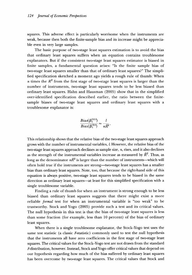
explanators. But if the consistent two-stage least squares estimator is biased in finite samples, a fundamental question arises: "Is the finite sample bias of

two-stage least squares smaller than that of ordinary least squares?" The simplified specification sketched a moment ago yields a rough rule of thumb: When n times the R2 from the first stage of two-stage least squares is larger than the number of instruments, two-stage least squares tends to be less biased than

ordinary least squares. Hahn and Hausman (2005) show that in the simplified over-identified specification described earlier, the ratio between the finite-

sample biases of two-stage least squares and ordinary least squares with a troublesome explanator is:

Bias(f3SLS) 1 Bias(P3Ls) nR2 "

This relationship shows that the relative bias of the two-stage least squares approach grows with the number of instrumental variables, 1. However, the relative bias of the

two-stage least squares approach declines as sample size, n, rises, and it also declines as the strength of the instrumental variables increase as measured by 122. Thus, as

long as the denominator nlR2 is larger than the number of instruments-which will often hold true if the instruments are strong-two-stage least squares has a smaller bias than ordinary least squares. Note, too, that because the right-hand side of this

equation is always positive, two-stage least squares tends to be biased in the same direction as ordinary least squares-at least for this simplified specification with a

single troublesome variable.

Finding a rule of thumb for when an instrument is strong enough to be less biased than ordinary least squares suggests that there might exist a more reliable formal test for when an instrumental variable is "too weak" to be

trustworthy. Stock and Yogo (2005) provide such a test and its critical values. The null hypothesis in this test is that the bias of two-stage least squares is less than some fraction (for example, less than 10 percent) of the bias of ordinary least squares.

When there is a single troublesome explanator, the Stock-Yogo test uses the same test statistic (a classic Fstatistic) commonly used to test the null hypothesis that the instruments all have zero coefficients in the first stage of two-stage least

squares. The critical values for the Stock-Yogo test are not drawn from the standard

Fdistribution, however. Instead, Stock and Yogo offer critical values that depend on our hypothesis regarding how much of the bias suffered by ordinary least squares has been overcome by two-stage least squares. The critical values that Stock and


Yogo calculate depend on the number of instruments, 1, and on the number of troublesome explanators.7

Biased Standard-Error Estimates in Two-Stage Least Squares The estimated variance of two-stage least squares is generally biased downward

in finite samples, and the bias can become quite large when the instruments are weak (Nelson and Startz, 1990a). Thus, weak valid instruments are likely to distort the significance levels usually claimed for tests based upon two-stage least squares- null hypotheses are too often rejected because the estimated variances are too small. Moreover, when instruments are weak, the asymptotic distribution of the two-stage least squares estimator is decidedly nonnormal (Stock, Wright, and Yogo, 2002).

Stock and Yogo (2005) show that the general approach that is suitable for assessing the reduction of bias achieved by two-stage least squares can be adapted to assessing the actual significance level of two-stage-least-squares-based hypothesis tests. The test statistics Stock and Yogo use in this application are the same ones they use to test the extent of bias reduction, but the critical values are different. As with Stock-Yogo tests about bias-reduction, the critical values for Stock-Yogo tests about the validity of usually stated significance levels depend on the number of instruments and the number of troublesome explanators, but these validity tests require less over-identification than do the tests about bias.8

When the Stock and Yogo (2005) tests reject the null hypothesis that valid instruments are weak, two-stage least squares coefficient estimates and their corresponding estimated standard errors are probably not much biased, and inference based on them is probably valid. A caveat is warranted here: if a researcher engages in pretesting for weak instruments, that pretesting changes the distribution of the two-stage least squares estimates that one finally examines. Andrews and Stock (2005) suggest foregoing two-stage least squares altogether because they prefer to avoid the potential pitfalls of pretesting. However, others may prefer to use two- stage least squares when the Stock-Yogo test indicates that their instruments are strong.

In Yogo's (2004) instrumental variable analysis of the intertemporal elas-

7As an example, consider the null hypothesis that the bias in two-stage least squares is less than 10 percent of the bias of ordinary least squares when there is a single troublesome explanator. For three instruments, Stock and Yogo (2005) report that the critical value of the classic Fstatistic is 9.08 for their test of this hypothesis. For four instruments, the corresponding critical value is 10.27. To test for reduced bias requires some over-identification; for example, the Stock-Yogo test for reduced bias cannot be conducted with fewer than three instruments when there is a single troublesome variable. When there are multiple troublesome variables, the Stock-Yogo test no longer relies on an Fstatistic, but on its multivariate generalization, the Cragg-Donald statistic, which is available in some software packages. SAs an example, consider the null hypothesis that the true significance level of hypothesis tests about

the troublesome explanators' coefficients is smaller than 10 percent when the usually stated significance level is 5 percent. For one instrument and a single troublesome explanator, Stock and Yogo (2005) report that the critical value of the classic Fstatistic is 16.38 for their test of this hypothesis. For two instruments, the corresponding critical value is 19.93. And for three instruments, the corresponding critical value is 22.30.


ticity of substitution, he conducts Stock-Yogo tests of both bias reduction and

significance-level distortion. He examines the weakness of his instruments in these regards both for the specification in which the real rate of return is the troublesome variable (the direct regression) and for the specification in which

consumption growth is the troublesome variable (the reverse regression). In Yogo's quarterly data, Stock-Yogo tests reveal that the real rate of return is

predictable enough for two-stage least squares applied to the direct regression to

provide relatively unbiased parameter estimates, but is not predictable enough to avoid distorted significance levels for tests based upon those two-stage least squares estimates. In contrast, Stock-Yogo tests reveal that consumption growth is so poorly predicted by the instrumental variables that the two-stage least squares estimates of the reverse regression are seriously biased, and tests based upon those estimates suffer seriously understated significance levels.

Yogo uses his test results to explain why economists using direct regressions and reverse regressions could get such puzzlingly different confidence intervals for the elasticity of intertemporal substitution. With weak instruments, two-stage least

squares yields inappropriately narrowed confidence intervals (and hence distorted

significance levels) for the intertemporal elasticity of substitution in both direct and reverse regressions. Moreover, those confidence intervals are apt to be centered

differently from one another because the former are almost unbiased, while the latter are markedly biased. In sum, Yogo's analysis shows that weak instruments have given rise to the puzzle about the size of the elasticity of intertemporal substitution.

Inference and Estimation with Weak Instruments

Two-stage least squares is a poor strategy for estimation and hypothesis testing when instruments are weak and the model is over-identified. Yogo's analysis highlights this point. That weak instruments can undermine two-stage least squares has been widely known since the works of Nelson and Startz (1990a, 1990b) and Bound, Jaeger, and Baker (1995). Having recognized the problem, economists then sought solutions. One thread of the search asked "What, exactly, are weak instruments, and how can we test for them?" This thread led to Stock and Yogo's tests for bias reduction and significance level distortion. A second thread of the search asked "How should researchers carry out inference and estimation when instruments are weak?" Recently, this thread has also made significant progress.

The state of the art for hypothesis testing with weak instruments and a single troublesome explanator is a "conditional likelihood ratio" test, developed by Moreira (2003) and explored further by Andrews, Moreira, and Stock (2006) and Andrews and Stock (2005).9 How does the conditional likelihood ratio test differ

9 Frank Kleibergen (2002) independently developed a testing strategy closely akin to Moreira's. I dwell on Moreira's approach in part because it is the tool Yogo uses and in part because the software for it is

readily available. A Stata command for implementing the two-sided conditional likelihood ratio test can be downloaded from within Stata. The programs are at Marcelo Moreira's Harvard website. If the disturbances in the original ordinary least squares regression are heteroskedastic or serially correlated,


from an ordinary instrumental-variable-based hypothesis test? Moreira's test over- comes the distortions of standard tests by adjusting the critical values for hypothesis tests from sample to sample so that, for given data, the critical values used yield a correct significance level. Thus, his critical values are "conditioned" on the data in hand, not constant. Andrews and Stock (2005) and Andrews, Moreira, and Stock

(2006) argue persuasively that the conditional likelihood ratio test should be the test of choice in over-identified instrumental variable applications when the instruments are weak and there is a single troublesome explanator. However, some users of two-stage least squares may prefer to stick with standard statistical tests when their instruments are strong. How best to conduct hypothesis-testing about the coefficients of a subset from among several troublesome variables when instruments are weak remains an open question, but Kleibergen (2004) and Dufour and Taamouti (2005; forthcoming) offer suggestions.

The conditional likelihood ratio test provides a strategy for constructing confidence intervals for the coefficient of a lone troublesome variable with weak instrumental variables: calculate the confidence interval as the set of coefficient

values that would not be rejected in Moreira's conditional likelihood ratio test at the desired level of statistical significance.'0 How to build valid confidence intervals when there are multiple troublesome explanators and weak instruments remains an open question.

Yogo (2004) uses a Moreira-style conditional likelihood ratio test in studying the intertemporal elasticity of substitution, P. With this approach, Yogo rejects the null hypothesis that P = 1 in each of the eleven countries that he studies. Yogo also uses Moreira's approach to construct confidence intervals for the intertemporal elasticity of substitution. Like the direct regression estimates obtained with two-

stage least squares, Yogo's conditional likelihood-based confidence intervals indicate that P is less than one. Thus, the results using the conditional likelihood ratio test support Yogo's finding using the Stock and Yogo (2005) critical values: two-

stage least squares is approximately unbiased when applied to the direct regressions of consumption growth on the real interest rate, but quite biased because of weak instruments when applied to indirect regressions of the real interest rate on

consumption growth. The conditional likelihood test provides a strong foundation for building

confidence intervals, but it does not provide point estimates. Theorists agree that

two-stage least squares performs badly in over-identified models when instruments are weak, but there has been debate about what point estimator to use instead.

then heteroskedasticity- and serial-correlation-robust versions of the conditional likelihood ratio test should be used to build confidence intervals. 10 The Stata routines for conducting conditional likelihood ratio (CLR) tests also offer CLR-based confidence intervals computed with an algorithm from Mikusheva (2005). Confidence intervals based on conditional likelihood ratios can have the unusual property of being made up of disjoint sets. See Murray (2005) for a discussion.


Increasingly, theorists endorse two of Fuller's (1977) estimators as the best choices (Andrews and Stock, 2005; Hahn, Hausman, and Kuersteiner, 2003).11

When Instruments are Both Weak and Invalid When an invalid instrument is "almost valid," that is when its nonzero covariance

with the errors is small in some suitable sense, is the consequent bias in two-stage least

squares also small? Strong and almost valid instruments do tend to bias two-stage least

squares only a little. However, weak instruments that are almost valid bias

two-stage least squares markedly more than do their strong counterparts (Hahn and Hausman, 2005). Consequently, weak instruments require giving particular attention to establishing the validity of instruments; "almost valid" might not do.

This observation has implications for an argument sometimes made when

lagged variable values are used as instruments. Analysts sometimes use longer lags of potential instruments on the supposition that the longer lags will provide a better instrument because a longer lag will reduce any correlation between the instrument and the disturbances in the error term of the original ordinary least squares regression. However, more distant lags are also more likely to be weakly correlated with the troublesome explanator, which means that using distant lags increases the

prospect that even "mild" invalidity in the instrument threatens to undermine the

credibility of the two-stage least squares estimates. Consequently, the case made for the validity of long-lagged variable values as instruments must be especially com-

pelling for such instrumental variable results to be credible.

The Next Big Thing: Heterogeneous Responses and Instrumental Variable Estimation

Presumably, states that lost prison overcrowding lawsuits wanted to lower their

prison populations judiciously, whenever possible releasing, or not imprisoning, criminals relatively disinclined to commit further crimes. Had those states instead reduced

prison populations by the same amount by pursuing a "Pity the Habitually Frequent Perpetrator" policy, in which particularly chronic offenders were released, the observed effect of lower incarceration rates on crime rates would probably have been consider-

ably larger than Levitt observed. The example is whimsical, but the point is substantial: the response of expected crime rates to lower incarceration rates is probably hetero-

geneous across states and times. Heterogeneous responses of the expected value of Y to changes in X pose problems for regression analyses in general and instrumental variable estimation in particular. If responses are heterogeneous, economists must decide what aspects of the distribution of responses are economically interesting and determine what econometric techniques can uncover those aspects of the responses (Angrist, Graddy, and Imbens, 2000).

1 These tests are available in Stata's ivreg2 command, namely those with the "Fuller parameter" set to 2 or 4.


In Levitt's work, one might argue that policymakers would usually shift prison populations much as did the states facing overcrowding lawsuits, in which case seeing how crime rates responded to changes in incarceration in those states might be instructive for officials elsewhere pondering new policies. But suppose Levitt's instrumental variable estimation had avoided ordinary least squares' bias by relying on some states having been randomly assigned to "Pity the Habitually Frequent Perpetrator" programs, instead of on haphazardly occurring overcrowding lawsuits. The resulting instrumental variable estimates would have probably overstated the responsiveness of crime rates to the sorts of policy changes that sensible state officials would follow. Generally, when an instrumental variable is correlated with heterogeneous responses, instrumental variable estimates will not reveal the mean

responsiveness, which is called the "average partial effect" (Wooldridge, 2002). The mean responsiveness across the population of all samples might, however, not even be the effect of economic interest. Instead, one might want to know, for example, the effect of changes in incarceration rates for a specific subset of the population. As Heckman, Urzua, and Vytlacil (2004, p. 2) write, "[I]n a heterogeneous response model, there is no guarantee that IV [instrumental variables] is any closer to the parameter of interest than OLS [ordinary least squares]."

Heterogeneous effects were first extensively studied in the context of dummy variable explanators, where the dummy variable indicates whether some experimental or programmatic treatment is applied to the observation (Imbens and Angrist, 1994). When responses are heterogeneous in such a model, the instrumental variable estimates are called "local average treatment effects." When Xis not a dummy variable, the instrumental variable estimators are said to estimate "local average partial effects" (Wooldridge, 2002, chap. 18). The word "local" refers to the fact that the instrumental variable estimator, in using only a portion of the variation in the Xvariable (the portion that accompanies variation in the instrument), might also restrict attention to a subset (a locale) of the responses to X.

Heckman, Urzua, and Vytlacil (2004, p. 2) point out: "In a model with essential heterogeneity, different instruments, valid for the homogeneous response model, identify different parameters. The right question to ask is 'what parameter or combination of parameters is being identified by the instrument?', not 'what is the efficient combination of instruments for a fixed parameter?', the traditional question addressed by econometricians." A recent spate of papers has begun advancing our knowledge of heterogeneous response models-including Heckman and Vyt- lacil (2005), Carneiro, Heckman, and Vytlacil (2005), and Heckman, Urzua, and Vytlacil (2004)-but much work remains to be done before social scientists will be as adept at grappling with heterogeneity as with instrument weakness or invalidity.

Conclusion

The barriers to Archimedes moving the earth with a lever were more daunting than the challenges facing instrumental variables estimation, but the comparison is apt. The perils of invalid and weak instruments open all instrumental variable estimates to


skepticism. Although instrumental variable estimation can be a powerful tool for

avoiding the biases that ordinary least squares estimation suffers when a troublesome

explanator is correlated with the disturbances, the work of Steven Levitt on policies to reduce crime and that of Motohiro Yogo on the intertemporal elasticity of substitution illustrate that applying instrumental variables persuasively requires imagination, dili-

gence, and sophistication. The discussion here of Levitt and Yogo's work yields three broad suggestions

for researchers about avoiding invalid instruments, coping with weak instruments, and interpreting instrumental variable estimates. First, subject candidate instruments to intuitive, empirical, and theoretical scrutiny to reduce the risk of using invalid instruments. We can never entirely dispel the clouds of uncertain validity that hang over instrumental variable analyses, but we should chase away what clouds we can. Second, because weak instruments can cripple two-stage least squares estimation in over-identified models, use "robust" instrumental variable procedures, such as the conditional likelihood ratio procedures and Fuller's estimators, whose good properties are not undermined by weak instruments, or, minimally, test candidate instruments for weakness before using them in vulnerable procedures like two-stage least squares. Third, before estimating a regression model, ask whether the behavioral responses one seeks to understand are markedly varied across one's population. If they are, carefully consider what aspects of those

responses are economically important and whether proposed instruments are likely to identify the behavior one wishes to understand.

We have also garnered insights into assessing both increases in the number of valid instruments and the use of mildly invalid instruments. Introducing additional valid instruments can decrease the standard error of the two-stage least squares estimator, but if the added instruments don't much increase /T2-the population correlation between the troublesome explanator and its first-stage fitted values-

they can also increase the finite-sample bias of two-stage least squares. The increase in bias can be large in even very large samples when the set of instruments as a whole is weak. Two-stage least squares can also suffer large finite-sample biases when the total number of instruments is large relative to the sample size.

In moderately large samples, strong instruments that are "almost valid" tend to

incur only small biases for two-stage least squares in moderately large samples. However, when "almost valid" instruments are weak, two-stage least squares can

suffer substantial biases. Biases due to almost valid instruments do not disappear as

the sample size grows. These findings suggest that the weaker one's instruments, the stronger one's validity arguments should be.

* Daron Acemoglu, Manuel Arellano, Bill Becker, Denise DiPasquale, Jerry Hausman, Jim Heckman, James Hines, Simon Johnson, Peter Kennedy, Jeff Kling, Marcelo Moreira, Jack Porter, Andre Shleifer, Carl Schwinn, Jim Stock, Michael Waldman, and Motohiro Yogo

provided helpful comments on drafts of this paper. Timothy Taylor edited the paper with

particular care. I am grateful to Vaibhav Bajpai for able research assistance.


References

Andrews, Donald W. K., Marcelo J. Moreira, and James H. Stock. 2005. "Optimal Invariant Similar Tests for Instrumental Variables Regres- sion with Weak Instruments." Cowles Founda- tion Discussion Paper No. 1476.

Andrews, Donald W. K., Marcelo J. Moreira, and James H. Stock. 2006. "Optimal Two-sided Invariant Similar Tests for Instrumental Vari- ables Regression." Econometrica. 74:3, pp. 715-52.

Andrews, Donald W. K., and James H. Stock. 2005. "Inference with Weak Instruments." Cowles Foundation Discussion Paper No. 1530.

Angrist, Joshua D., Katherine Graddy, and Guido W. Imbens. 2000. "Instrumental Variables Estimators in Simultaneous Equations Models with an Application to the Demand for Fish." Review of Economic Studies. 67:3, pp. 499-527.

Angrist, Joshua D. and Alan B. Krueger. 2001. "Instrumental Variables and the Search for Iden- tification: From Supply and Demand to Natural Experiments." Journal of Economic Perspectives. 15:4, pp. 69-85.

Arellano, Manuel, Lars P. Hansen, and En-

rique Sentana. 1999. "Underidentification?" Un- published paper, July.

Bound, John, David Jaeger, and Regina Baker. 1995. "Problems with Instrumental Variables Es- timation When the Correlation Between the In- struments and the Endogenous Explanatory Variable is Weak." Journal of the American Statisti- cal Association. 90:430, pp. 443-450.

Campbell, John Y. and Lucia M. Viceira. 2002. Strategic Asset Allocation: Portfolio Choice for Long- Term Investors. Clarendon Lectures in Econom- ics. New York: Oxford University Press.

Carneiro, Pedro, James J. Heckman, and Ed- ward Vytlacil. 2005. "Understanding What In- strumental Variables Estimate: Estimating Mar- ginal and Average Returns to Education." Unpublished paper.

Dufour, Jean-Marie, and Mohamed Taamouti. 2005. "Projection-Based Statistical Inference in Linear Structural Models with Possibly Weak In- struments." Econometrica. 73:4, pp. 1351-65.

Dufour, Jean-Marie and Mohamed Taamouti. Forthcoming. "Further Results on Projection- Based Inference in IV Regressions with Weak, Collinear or Missing Instruments." Journal of Econometrics.

Epstein, Larry G. and Stanley E. Zin. 1989. "Substitution, Risk Aversion, and the Temporal Behavior of Consumption and Asset Returns: A Theoretical Framework." Econometrica. 57:4, pp. 937-69.

Fuller, Wayne A. 1977. "Some Properties of a Modification of the Limited Information Maxi-

mum Likelihood Estimator." Econometrica. 45:4, pp. 939-54.

Hahn, Jinyong and Jerry Hausman. 2005. "In- strumental Variable Estimation with Valid and Invalid Instruments." Unpublished paper, Cam- bridge, MA, July.

Hahn, Jinyong, Jerry Hausman, and Guido Kuersteiner. 2004. "Estimation with Weak In- struments: Accuracy of Higher Order Bias and MSE Approximations." Econometrics Journal. 7:1, pp. 272-306.

Hall, Robert E. 1988. "Intertemporal Substitu- tion in Consumption." Journal of Political Econ- omy. 96:2, pp. 339-57.

Hansen, Christian, Jerry Hausman, and Whit- ney Newey. 2005. "Estimation with Many Instru- mental Variables." Unpublished paper, Cam- bridge MA, July.

Hansen, Lars P. and Kenneth J. Singleton. 1983. "Stochastic Consumption, Risk Aversion, and the Temporal Behavior of Asset Returns." Journal of Political Economy, 91:2, pp. 249-65.

Heckman,JamesJ., Sergio Urzua, and Edward Vytlacil. 2004. "Understanding Instrumental Variables in Models with Essential Heterogene- ity." Unpublished paper.

Heckman, JamesJ. and Edward Vytlacil. 2005. "Structural Equations, Treatment Effects and Econometric Policy Evaluation." Econometrica. 73:3, pp. 669-738, May.

Hirsch, E. Donald, Joseph. F. Kett, and James Trefil. 2002. The New Dictionary of Cultural Liter- acy, 3rd Edition. Houghton Mifflin Company.

Imbens, Guido and Angrist, Joshua D. 1994. "Identification and Estimation of Local Average Treatment Effects. Econometrica. 62:2, pp. 467- 76.

Kleibergen, Frank. 2002. "Pivotal Statistics for Testing Structural Parameters in Instrumental Variables Regression." Econometrica. 70:5, pp. 1781-1803.

Kleibergen, Frank. 2004. "Testing Subsets of Structural Parameters in the Instrumental Vari- ables Regression Model." Review of Economics and Statistics. 86:3, pp. 418-23.

Leamer, Edward E. 1978. Specification Searches: Ad Hoc Inference with Non-Experimental Data. New York, NY: John Wiley and Sons.

Levitt, Steven D. 1996. "The Effect of Prison

Population Size on Crime Rates: Evidence from Prison Overcrowding Litigation." Quarterly Jfour- nal of Economics. 111:2, pp. 319-51.

Levitt, Steven D. 1997. "Using Electoral Cycles in Police Hiring to Estimate the Effect of Police on Crime." American Economic Review. 87:4, pp. 270-90.


Levitt, Steven D. 2002. "Using Electoral Cycles in Police Hiring to Estimate the Effect of Police on Crime: Reply." American Economic Review. 92:4, pp. 1244-50.

McCrary, Justin. 2002. "Using Electoral Cycles in Police Hiring to Estimate the Effect of Police on Crime: Comment." American Economic Review.

92:4, pp. 1236-43. Miller, Alan J. 1990. Subset Selection in Regres-

sion. New York: Chapman-Hall. Mikusheva, Anna. 2005. "An Algorithm for

Constructing Confidence Intervals Robust to Weak Instruments." Unpublished paper, Cam-

bridge, MA, October. Moreira, Marcelo J. 2003. "A Conditional

Likelihood Test for Structural Models." Econo- metrica. 71:4, pp. 1027-48.

Moreira, Marcelo J. 2005. "Tests with Correct Size When Instruments Can Be Arbitrarily Weak." Unpublished paper, Cambridge, MA, July.

Murray, Michael P. 2005. "The Bad, the Weak, and the Ugly: Avoiding the Pitfalls of Instrumen- tal Variables Estimation." Social Science Re- search Network Working Paper No. 843185.

Murray, Michael P. 2006. Econometrics: A Mod- ern Introduction. Boston: Addison-Wesley.

Nelson, Charles R. and Richard Startz. 1990a. "The Distribution of the Instrumental Variables Estimator and Its t-Ratio When the Instrument Is a Poor One." Journal of Business. 63:1, pt. 2, pp. S125-S140.

Nelson, Charles R. and Richard Startz. 1990b. "Some Further Results on the Exact Small Sam-

ple Properties of the Instrumental Variables Es- timator." Econometrica. 58:4, pp. 967-76.

Phillips, Peter C. B. 1983. "Exact Small Sam- ple Theory in the Simultaneous Equations Model," in Handbook of Econometrics. Vol. 1. Zvi Griliches and Michael D. Intriligator, eds. Elsevier, pp. 449-516.

Rothenberg, Thomas J. 1983. "Asymptotic

Properties of Some Estimators in Structural Models," in Studies in Econometrics, Time Series, and Multivariate Statistics, in honor of T. W. Anderson. Samuel Karlin, Takeshi Amemiya, and Leo A. Goodman, eds. Academic Press,

pp. 297-405. Rothenberg, ThomasJ. 1984. "Approximating

the Distributions of Econometric Estimators and

Test Statistics," in Handbook of Econometrics. Vol. 2. Zvi Griliches and Michael D. Intriligator, eds. Elsevier, pp. 881-935.

Sargan, J. Denis. 1958. "The Estimation of Economic Relationships with Instrumental Vari- ables." Econometrica. 26:3, pp. 393-415.

Staiger, Douglas and James H. Stock. 1997. "Instrumental Variables Regressions with Weak Instruments." Econometrica. 65:3, pp. 557-86.

Stock, James H., and Mark W. Watson. 2003. Introduction to Econometrics. Boston, MA: Addison-

Wesley. Stock, James H. and Motohiro Yogo. 2005.

"Testing for Weak Instruments in IV Regres- sion," in Identification and Inference for Econometric Models: A Festschrift in Honor of Thomas Rothenberg. Donald W. K. Andrews andJames H. Stock, eds.

Cambridge University Press, pp.80-108. Stock, James H.,Jonathan H. Wright, and Mo-

tohiro Yogo. 2002. "A Survey of Weak Instru- ments and Weak Identification in Generalized

Method of Moments," Journal of Business and Economic Statistics. 20:4, pp. 518-29.

Woodford, Michael D. 2003. Interest and Prices: Foundations of a Theory of Monetary Policy. Prince- ton: Princeton University Press.

Wooldridge, Jeffrey M. 2002. Econometric Anal-

ysis of Cross Section and Panel Data. Cambridge, MA: MIT Press.

Yogo, Motohiro. 2004. "Estimating the Elastic-

ity of Intertemporal Substitution When Instru- ments are Weak." Review of Economics and Statis- tics. 86:3, pp. 797-810.

avoiding invalid instruments and coping with weak instruments - smu

Documents