Research Report Agreement T2695, Task 38

AVL Vehicles as Speed Probes

AVL-Equipped Vehicles as Speed Probes

(Final Phase)

By

Daniel J. Dailey Professor

University of Washington Dept. of Electrical Engr.

Seattle, Washington 98195

Fredrick W. Cathey Research Scientist

University of Washington Dept. of Electrical Engr.

Seattle, Washington 98195

Washington State Transportation Center (TRAC)

Univeristy of Washington, Box 354802 University District Building, Suite 535

1107 N.E. 45th Street Seattle, Washington 98105-4631

Washington State Department of Transportation

Technical Monitor Pete Briglia

ITS Program Manager

Sponsored by

Washington State Transportation Commission Department of Transportation

Olympia, Washington 98504-7370

Transportation Northwest (TransNow) University of Washington 135 More Hall, Box 352700

Seattle, Washington 98195-2700

in cooperation with U.S. Department of Transportation

Federal Highway Administration

June 2005

TECHNICAL REPORT STANDARD TITLE PAGE1. REPORT NO. 2. GOVERNMENT ACCESSION NO. 3. RECIPIENT'S CATALOG NO.

WA-RD 617.1

4. TITLE AND SUBTITLE 5. REPORT DATE

AVL-EQUIPPED VEHICLES AS SPEED PROBES (FINAL June 2005PHASE) 6. PERFORMING ORGANIZATION CODE

7. AUTHOR(S) 8. PERFORMING ORGANIZATION REPORT NO.

Daniel J. Dailey and Fredrick W. Cathey

9. PERFORMING ORGANIZATION NAME AND ADDRESS 10. WORK UNIT NO.

Washington State Transportation Center (TRAC)University of Washington, Box 354802 11. CONTRACT OR GRANT NO.

University District Building; 1107 NE 45th Street, Suite 535 Agreement T2695, Task 38Seattle, Washington 98105-463112. SPONSORING AGENCY NAME AND ADDRESS 13. TYPE OF REPORT AND PERIOD COVEREDResearch OfficeWashington State Department of TransportationTransportation Building, MS 47372

Final Research Report

Olympia, Washington 98504-7372 14. SPONSORING AGENCY CODE

Doug Brodin, Project Manager, 360-705-797215. SUPPLEMENTARY NOTES

This study was conducted in cooperation with the U.S. Department of Transportation, Federal HighwayAdministration.16. ABSTRACT

The Washington State Department of Transportation (WSDOT) operates a central trafficmanagement system (TMS) for both day-to-day surveillance and traveler information. Past effortsdeveloped the ability to create real-time traffic speed information by using virtual sensors that are based ontransit vehicle tracking data. In order for this new information source to be merged into the TMS, anumber of questions, such as probe density in time and space, needed to be resolved.

This report presents the solution developed at the University of Washington (UW). This solutionprovides real-time congestion information from Seattle area freeways and arterials—I-5, I-90, SR 520 andSR 99—to the WSDOT TMS using the Intelligent Transportation System (ITS) Backbone. This projectharvests existing automatic vehicle location (AVL) data from within King County Metro Transit andtransports the raw data to the UW, where a series of operations converts the data into roadway speedinformation. This roadway speed information is color coded on the basis of specific, localized conditionsfor the arterials and freeways to reflect traffic congestion. The resulting traffic data product is thenprovided to WSDOT as a data source for virtual sensors located in roadways where currently there are noinductance loops.

In addition to creating the infrastructure for an AVL-equipped fleet to serve as probe vehicles, thisproject created several user interfaces for traveler information. One is “StoreView,” a Java application thatdisplays the spatial and temporal average speeds of transit vehicles as color-coded bubbles on a map of thearea’s major arterials and freeways. A second type of traveler information, analogous to TrafficTV andWSDOT’s pictographic traffic maps, is also available.

This report documents both the technical issues addressed in creating a virtual sensor data streamfrom probe vehicle data and the creation of a set of real-time traveler information applications.

17. KEY WORDS 18. DISTRIBUTION STATEMENT

Bus, transit, probe, GIS, AVL, virtual sensors, trafficprobes, transit probes, speed sensors, geographicinformation systems, road traffic, traffic control,traffic engineering computing, transportation

No restrictions. This document is available to thepublic through the National Technical InformationService, Springield, VA 22616

19. SECURITY CLASSIF. (of this report) 20. SECURITY CLASSIF. (of this page) 21. NO. OF PAGES 22. PRICE

None None

DISCLAIMER The contents of this report reflect the views of the authors, who are responsible for

the facts and the accuracy of the data presented herein. This document is disseminated

through the Transportation Northwest (TransNow) Regional Center under the sponsorship of

the U.S. Department of Transportation UTC Grant Program and through the Washington

State Department of Transportation. The U.S. government assumes no liability for the

contents or use thereof. Sponsorship for the local match portion of this research project was

provided by the Washington State Department of Transportation. The contents do not

necessarily reflect the official views or policies of the U.S. Department of Transportation or

Washington State Department of Transportation. This report does not constitute a standard,

specification, or regulation.

iii

iv

TABLE OF CONTENTS

EXECUTIVE SUMMARY ....................................................................................................................VII

1. INTRODUCTION............................................................................................................................1

2. VIRTUAL SENSORS: SPATIAL AND TEMPORAL SELECTION.........................................4

2.1 New Interval Speed Estimates......................................................................................... 8 2.2 New “Store” Component................................................................................................. 8 2.3 New Transmitter Component ........................................................................................ 10 2.4 Summary: Virtual Sensors for Traffic Surveillance ...................................................... 12

3. PROBEVIEW.................................................................................................................................13

3.1 Using ProbeView .......................................................................................................... 13 3.2 Software Architecture (Detail) ...................................................................................... 15

3.2.1 ProbeModel .......................................................................................................................15 3.2.2 ProbeCanvas .....................................................................................................................16 3.2.3 ProbeView .........................................................................................................................17

4. STOREVIEW.................................................................................................................................18

5. GIF WRITER.................................................................................................................................20

6. TRAVELTIME WEB PAGE........................................................................................................23

7. PICTOGRAPHIC MAP FOR VIRTUAL SENSOR SPEEDS ..................................................25

8. CONCLUSIONS ............................................................................................................................26

REFERENCES .........................................................................................................................................27

v

LIST OF FIGURES

Figure 1: Virtual Sensor Backbone....................................................................................................... 2

Figure 2: Map of roadways in Seattle. Requested virtual sensors on the left. Sensors with suitable coverage on the right. ......................................................................................................... 4

Figure 3: Headway window versus number of useful sensors. ............................................................. 5

Figure 4: Application as collaborative components.............................................................................. 7

Figure 5: Virtual sensor data from the ProbesStore every 20 seconds over the course of a day. ....... 10

Figure 6: Histogram for two months of speed data at one virtual sensor (2,592 observations).......... 11

Figure 7: ProbeView user interface .................................................................................................... 14

Figure 8: StoreView user interface ..................................................................................................... 19

Figure 9: GIFWriter area selection page............................................................................................. 20

Figure 10: GIFWriter speed page........................................................................................................ 21

Figure 11: TravelTime list page.......................................................................................................... 23

Figure 12: Virtual sensor traffic congestion map based on the use of transit vehicles as traffic probes................................................................................................................................ 25

LIST OF TABLES

Table 1: Example of period of continuous functionality ..................................................................... 6

vi

EXECUTIVE SUMMARY

The Washington State Department of Transportation (WSDOT) operates a central

traffic management system (TMS) for both day-to-day surveillance and traveler information.

Past efforts developed the ability to create real-time traffic speed information by using

virtual sensors that are based on transit vehicle tracking data. In order for this new

information source to be merged into the TMS, a number of questions, such as probe density

in time and space, needed to be resolved.

This report presents the solution developed at the University of Washington (UW).

This solution provides real-time congestion information from Seattle area arterials and

freeways—I-5, I-90, SR 520 and SR 99—to the

WSDOT TMS using the Intelligent Transportation

System (ITS) Backbone, as shown in Figure ES1.

This project harvests existing automatic vehicle

location (AVL) data from within King County Metro

Transit and transports the raw data to the UW, where

a series of operations converts the data into roadway

speed information. This roadway speed information

is color coded on the basis of specific, localized

conditions for the arterials and freeways to reflect

traffic congestion. The resulting traffic data product

is then provided to WSDOT as a data source for

virtual sensors located in roadways where presently

there are no inductance loops.

Figure ES1: ITS Backbone

In addition to creating the infrastructure for

an AVL-equipped fleet to serve as probe vehicles,

this project created several user interfaces for

traveler information. One is “StoreView,” a Java

application that displays the spatial and temporal

average speeds of transit vehicles as bubbles on a

map of the major arterials and freeways. The bubbles

are color-coded to reflect the local traffic conditions

vii

(see Figure ES2). This

application can be found at:

http://www.its.washington.edu/

storeview/storeview.jnlp

Another type of traveler

information, analogous to

TrafficTV and WSDOT’s

pictographic traffic maps, is

also available. This interface is

shown in Figure ES3 and can

be found at:

http://www.its.washington.edu/

probes_traffic/

This report documents

both the technical issues

addressed in creating a virtual

sensor data stream from probe

vehicle data and the creation of

a set of real-time traveler

information applications.

Figure ES2: StoreView

Figure ES3: Virtual sensor traffic congestion map based on the use of transit vehicles as traffic probes.

viii

1. INTRODUCTION

The Washington State Department of Transportation (WSDOT) performs congestion

monitoring with a network of several thousand inductance loops deployed on the freeways

and occasional arterials around Seattle. However, on some important corridors it is not

possible, for political and fiscal reasons, to install inductance loops. To overcome this

obstacle, the authors have described, in previous papers, the technology to create virtual

sensors by using the automatic vehicle location (AVL) system operated by King County

Metro Transit for fleet management [1, 2]. The AVL data are extracted from the AVL

system and transferred to the University of Washington for processing into traffic probe

data. Dailey and Cathey [3, 4] described a Kalman filter approach [5, 6, 7, 8, 9] to make an

optimal point speed estimate from the AVL observations as the vehicles pass over the virtual

sensors. These estimates compared favorably with inductance loop data from the freeways

and, just as with inductance loops, can be used to detect incidents. The speed estimates, in

turn, can be used to estimate corridor travel times by integrating a speed function over space

and time [10].

The logical extension of this work was to create speed estimates on the un-

instrumented arterials and make those data available to WSDOT. This involved some

additional technical work: (1) algorithms to refine the speed estimate, (2) identification of

suitable corridors and sites that would provide usable amounts of data, and (3)

implementation of some additional Intelligent Transportation System (ITS) Backbone [11,

12] components.

The probe vehicle-related ITS Backbone components are shown in Figure 1 as taken

from documentation on the ITS Backbone, http://www.its.washington.edu/mdi/status_scripts

/images/page2.htm. The AVL data are shown at the top as starting at a source component

“AVLUW2,“ and the various products are shown as sink components at the bottom. This

report describes the technical efforts necessary to make the virtual sensor data suitable and

available to WSDOT through the ITS Backbone. In addition, a number of user interfaces to

this data stream were developed and deployed on the University of Washington (UW) ITS

website.

1

Figure 1: Virtual Sensor Backbone

This report first describes the effort to provide a new data stream, based on virtual

sensors constructed by using transit vehicles as probes, to WSDOT’s Traffic Systems

Management Center (TSMC) for use in the traffic management system (TMS). This data

stream is indicated by the second sink from the left at the bottom of Figure 1, labeled

“WSDOT TMS Harley.”

In addition, this report describes alternative application/user interfaces that

demonstrate the use of virtual sensors, based on transit vehicles as probes, for traveler

information. These additional applications/user interfaces include the following:

• ProbeView is a Java applet that displays vehicle speed as vehicles pass a set of

virtual sensors scattered about the Seattle metro area.

http://www.its.washington.edu/probeview/probeview.jnlp

2

• StoreView is a Java applet that displays time and spatially averaged speeds for

selected locations on SR 99, I-5, SR 520 and I-90.

http://www.its.washington.edu/storeview/storeview.jnlp

• GIFWriter is a set of GIF images captured from a set of regions-of-interest covering

the Puget Sound area.

http://www.its.washington.edu/transit-probes/

• TravelTime Page is a Web page with travel times for selected routes in the Seattle

metro area.

http://www.its.washington.edu/probes/traveltimes/

• Pictographic Traffic Map is a traffic map GIF based on probe vehicles and is

analogous to the traffic map found on TrafficTV but also includes SR 99.

http://www.its.washington.edu/probes_traffic/

The set of applications and interfaces documented in this report demonstrates the

viability of using an AVL-equipped fleet as a regional traffic surveillance system suitable

for both traveler information and traffic management. While these ideas were implemented

in King County with the King County Metro transit fleet AVL system as input, the

underlying concept may be generalized to any area where a fleet of vehicles is tracked in

real time.

3

2. VIRTUAL SENSORS: SPATIAL AND TEMPORAL SELECTION

One relatively un-instrumented facility of interest for WSDOT was State Route 99

(SR 99), which parallels Interstate 5 (I-5) in Seattle. Initially, sensors were requested

halfway between signalized intersections for major arterials, or about every ten blocks (see

Figure 2. left). The data stream flowing through the components contains data for all of

these virtual sensors. However, it was not possible to use all these virtual sensors with the

TMS because of constraints on the transit schedule.

Figure 2: Map of roadways in Seattle. Requested virtual sensors on the left. Sensors with suitable coverage on the right.

WSDOT personnel desired continuous temporal coverage. To evaluate the temporal

coverage, the authors examined the schedule database. Bus headways in Seattle are rarely

less than 15 minutes on individual routes; however, many routes operate on the chosen

facility, SR 99. Because of the variability of the speed estimate from any single vehicle, it

4

was decided that at least two speed estimates should be averaged to provide the speed

estimate for WSDOT. This would create a sliding time window during which two reports

from vehicles would likely be observed. There was a tradeoff between the length of this time

window and the number of virtual sensors that would qualify as “useful.” When the schedule

was examined for each sensor location using the criteria that (1) there must be at least two

vehicles scheduled within the selected time window, and (2) there must be at least 20 time

windows in a row for which this was true, we were able to qualify some number of virtual

sensors as useful. The second criterion of sequential time windows arose from WSDOT’s

requirement that for a sensor to be “useful,” it must operate continuously for a reasonable

period of time. Twenty sequential windows guaranteed that a sensor would operate

continuously for over an hour. Figure 3 is a plot of the number of useful sensors in the

corridor versus the duration of the time window for the transit service scheduled for winter

2004-2005.

Figure 3: Headway window versus number of useful sensors.

A time window of 9 minutes was selected for time-averaging the transit vehicle

reports. Note that the criteria for being a useful sensor only required that it operate

continuously over a relatively short period. As it happens, the scheduled trips that met the

criteria occurred during the morning/southbound and evening/northbound commute periods.

5

Table 1 shows the periods of continuous operation on the northbound and southbound

roadways of SR 99. Note that within the downtown area (sensors 31-38) monitoring

occurred continuously in both the morning and afternoon. Data from some buses outside of

these windows could have been used by the virtual sensors, but there would also have been

periods when no information about traffic speed would have been acceptable, given the

“useful” criteria.

Table 1: Example of period of continuous functionality

Southbound

Sensor Start Time End Time 2 6.61 8.51 3 6.42 8.31

15 6.92 8.71 16 6.93 8.72 17 6.48 9.26 18 6.49 9.27 19 6.51 9.29 20 6.52 9.30 21 6.54 9.31 22 7.04 9.33 23 7.05 9.33 31 7.45 9.56 31 11.36 17.85 32 7.20 9.57 32 11.38 17.86 33 7.20 9.57 33 11.38 17.86 34 7.23 9.59 34 11.39 17.88 35 7.23 9.59 35 11.39 17.89 36 7.24 9.60 36 11.40 17.90 37 7.24 9.60 37 11.40 17.90 38 7.26 9.62 38 11.42 17.92

Northbound

Sensor Start Time End Time 2 17.19 18.74 3 17.10 18.70

36 7.50 8.87 36 16.57 18.31 37 7.50 8.87 37 16.57 18.31 38 7.48 8.85 38 16.55 18.29 72 7.51 8.88 72 16.58 18.32 73 7.51 8.89 73 16.58 18.32 74 7.52 8.91 74 16.59 18.33 75 7.53 8.91 75 16.60 18.33 76 7.54 8.99 76 16.11 18.34 77 7.55 9.40 77 16.11 18.35 84 13.13 18.30 85 13.14 18.30 86 6.28 7.88 86 13.10 18.90 87 6.29 7.90 87 13.12 18.91 88 6.39 7.91 88 13.14 18.93 89 6.40 7.92 89 13.15 18.94 90 6.41 7.68 90 13.17 15.95 90 16.10 18.95 91 16.83 18.07 92 16.84 18.07

6

The traffic management community is accustomed to having sensors report at fixed

intervals. The WSDOT polls inductance loops, intersection master controllers, and traffic

counters at intervals of from 20 seconds to 15 minutes. However, the virtual sensors created

with probe vehicles only update when a vehicle passed the location assigned to the virtual

sensor. This created the need for new components for the Traffic Probes application. The

software that implements the “transit vehicle as traffic probes” concept was built in a

modular manner and is made up of collaborating components, running on several computers,

shown as individual boxes in Figure 4. Each component has a name, port, and computer

name (Figure 4), and self-describing data (SDD) [11] flow between the components on the

TCP ports indicated on the figure. Each component performs a specific operation on the data

flow. For example, the component labeled Tracker implements the Kalman filter described

by Dailey and Cathey [3]. To support the additional requirements of integrating these data

into the transportation management framework, three additional components, shown in bold

in Figure 3, were added: Interval Probes, ProbesStore and TMSServer.

Figure 4: Application as collaborative components.

7

2.1 New Interval Speed Estimates

In past work, the authors created virtual sensor reports only when a vehicle passed

the exact geographic location of the virtual sensor [3]. In an effort to create both more

accurate speed estimates and more frequent speed estimates, the project used the notion of

an interval along the roadway around the virtual sensor to select the probe vehicle reports

that would be associated with a specific virtual sensor.

To accomplish this, the researchers used a geographic information system (GIS)

graph of arcs and nodes that represented the road system of King County. With this graph

we created “corridors” that were directed paths or sequences of adjacent arcs that covered

freeways and arterials (e.g., SR 99, I-5, I-90)

“Virtual sensors” and “probe intervals” are distributed along the corridors. A virtual

sensor location is specified by an arc and its distance from the start of the arc. The location

of a virtual sensor on a corridor is determined by its distance from the start point of the

corridor. Non-overlapping adjacent linear intervals are constructed around each virtual

sensor location on each corridor.

For each transit AVL report, the software determines which corridor the vehicle is

on, if any, and which probe interval it is in. The speed of the vehicle is estimated in the

component labeled AvlTracker2.

This speed estimate is a member of the data structure for the AVL report. As the

vehicle travels along the corridor, its position may change from one interval to another or

stay in the same interval. For each AVL report, virtual sensor speed reports are output for

the interval the vehicle is in, and interpolated speed reports are output for intermediate

intervals traversed since the last report.

The component Interval Probes (see Figure 4) implements the spatial expansion of

the virtual sensor to an interval of roadway. These data are averaged in the downstream

ProbesStore component to create speed estimates from a region of the roadway and an

interval of time. Increasing the number of vehicle speed estimates used to create an estimate

of roadway speed improves the confidence in the roadway estimate.

2.2 New “Store” Component

The ProbesStore component was added to support the averaging of the vehicle speed

data over the selected time window. In addition, it implements the selection of specific

8

sensors and maps the virtual sensors into the data structures required by the TMS. The TMS

uses the notion of “Cabinets,” which are both physical roadside cabinets that hold the

inductance loop equipment and a data structure in the TMS software that stores the loop

data.

The ProbesStore component has two parts, an SDD receiver and a request/response

server. The SDD receiver obtains the probe data, in SDD format, that is made up of the

probe ID, the direction of travel, the time, the speed, and the vehicle ID. The server responds

to data requests from the TMSServer.

At startup, the ProbesStore component obtains the list of sensors requested by

WSDOT from a file. This file ties the virtual sensor information to the notion of a “cabinet,”

a data structure in the TMS that uses: probe ID, roadway, road type, cross street, mile

markers, corridor, x, y, and cabinet ID. There is a unique sensor ID for each roadway and

direction pair, and several sensor IDs are associated with a cabinet ID, much as several loops

(e.g., northbound, southbound, and reversible) are assigned to a cabinet.

Using the list of sensors, ProbesStore creates a hash table to contain the actual

reports received. As ProbesStore receives a sensor report, it uses the hash key to look up the

appropriate record, prunes the list of reports to include only the reports in the last nine

minutes, adds the new report, and sets the last update time for that sensor.

The server side of ProbesStore waits for requests, and upon receiving a request, it

prunes the list for the sensors to enforce the time window, computes the average speed, and

sends the appropriate report containing sensor ID, direction, road type, count, speed, number

of vehicle IDs, and the time since last update.

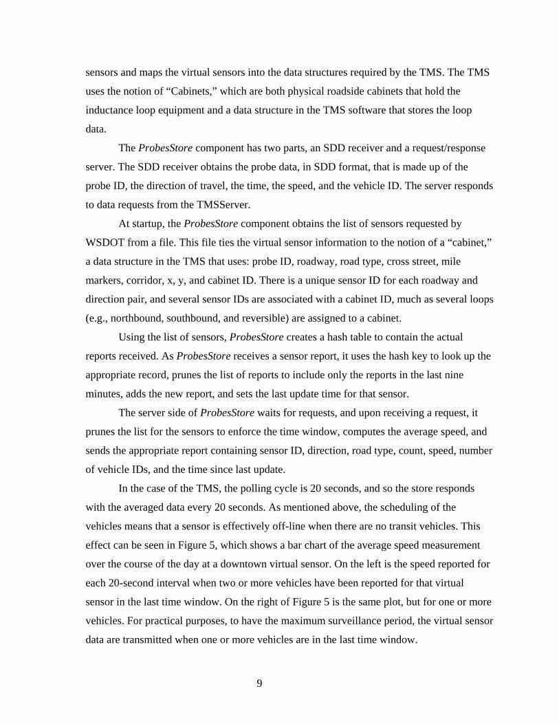
In the case of the TMS, the polling cycle is 20 seconds, and so the store responds

with the averaged data every 20 seconds. As mentioned above, the scheduling of the

vehicles means that a sensor is effectively off-line when there are no transit vehicles. This

effect can be seen in Figure 5, which shows a bar chart of the average speed measurement

over the course of the day at a downtown virtual sensor. On the left is the speed reported for

each 20-second interval when two or more vehicles have been reported for that virtual

sensor in the last time window. On the right of Figure 5 is the same plot, but for one or more

vehicles. For practical purposes, to have the maximum surveillance period, the virtual sensor

data are transmitted when one or more vehicles are in the last time window.

9

Figure 5: Virtual sensor data from the ProbesStore every 20 seconds over the course of a day.

2.3 New Transmitter Component

The final new component is the TMSServer. This component listens for requests

from the TMS and responds to the TMS with virtual sensor data. The TMS polls all of the

field equipment every 20 seconds. When the poll is received, the TMSServer makes a

request to ProbesStore for the virtual sensor data and relays them to the TMS.

The TMS was designed to handle inductance loop data in two forms. The first form

is that of a “loop,” in which the information is (1) “volume,” number of vehicles passing

over the loop, and (2) “scan count,” the number of 1/60th-second scans of the loop in the last

20 seconds that the loop had a vehicle above it. The second form of TMS data is a “speed

trap,” which consists of two physical loops, but the data reported are average speed and

average length. WSDOT requested that the virtual sensor data be cast into the “loop” data

structure. Furthermore, the TMS uses a derivative of the scan count, “occupancy,” the

fraction of time that the loop is covered by a vehicle, as the measure of congestion, and it

creates a traffic condition map based on thresholds on the occupancy.

The “loop” structure does not contain any notion of speed. However, the authors

desired a painted traffic map similar to the existing occupancy-based map. The existing map

has three thresholds for occupancy: green (1-15 percent), yellow (16-22 percent), and red

(22-30 percent).

To create a similar quantization for the virtual sensors, the researchers created

histograms for the selected sensors along SR 99. Figure 6 shows the histogram for two

months of data for the same virtual sensor used in Figure 5. We concluded from examining

10

the resulting histograms that it was unrealistic to obtain a tri-modal distribution from the

virtual sensor data. Instead, a bimodal distribution is proposed—congested and

uncongested—with a distribution boundary at 30 miles per hour for the example sensor.

Because of the different road geometries found on arterials, an analysis of the

probability distribution for each sensor was used to create a threshold between the two

modes for that sensor. The modes corresponded to red and green for the TMS traffic map.

Using a threshold on the probe vehicle speed, we assigned one of three values to the scan

count: (1) Scan count equal to zero indicates that no probe vehicles passed in the last time

window. (2) WSDOT defines congested as more than 22 percent occupancy, and under these

conditions it would paint the congestion map red. To be conservative, this would be

equivalent to a scan count of 300 for the sensor described above, and so, when the example

virtual sensor speed drops below 30 MPH, the scan count is set to 300. (3) When the

example virtual sensor speed is greater than 30 MPH, the scan count is set to 120, and the

TMS paints the traffic map green in the region of the virtual sensor. The volume is set to the

number of vehicles observed in the interval of the virtual sensor for the last time window. In

this way, the virtual sensor data are reformatted so that they can be used by the existing

TMS applications for traffic management and traveler information without any software

changes by WSDOT. This incorporates the virtual sensor system into the TMS.

Figure 6: Histogram for two months of speed data at one virtual sensor (2,592 observations).

11

2.4 Summary: Virtual Sensors for Traffic Surveillance

This project created an application that expands the sensing capabilities of the

Washington State DOT to areas where it does not have installed infrastructure. Past work

has described algorithms to create virtual sensors on arterials and freeways by using existing

transit vehicles. This section described modifications to the algorithms necessary to allow

the virtual sensors to be used in the existing traffic management system in Seattle. It

examined the transit schedule and proposed criteria for selecting virtual sensors that are

“useful” to the TMS. This section also documented a threshold that WSDOT uses to paint a

traffic map, and it described the overall framework that will provide WSDOT with expanded

surveillance capabilities by reusing data from another agency with algorithms from the

University of Washington.

12

3. PROBEVIEW

ProbeView is an interface to the virtual sensor data that displays the vehicle speed as

vehicles pass a set of virtual sensors scattered about the Seattle metropolitan area.

http://www.its.washington.edu/probeview/probeview.jnlp

ProbeView was built as a Java Swing application that provides a map-based view of a

real-time probe data stream. It was configured to run as a Java Webstart application and may

be accessed from the ITS UW Web server. The application displays the roads traversed by

King County Metro transit vehicles, probe sensor locations, and current vehicle speeds. In

addition, probe data history can be displayed for any selected probe sensor location.

3.1 Using ProbeView

The application opens with a default viewport showing a rectangular region of an

underlying “canvas” on which are painted the roadways, sensor locations, and speed

bubbles. The default scaling is approximately 60 feet per pixel, or 1 mile per inch on a high-

resolution display. Scrollbars on the bottom and right side of the display enable the user to

scroll over the canvas. A right-button click of the mouse at given canvas points will pop up a

menu of zoom options: zoom-in, zoom-out, reset, and rubberband (see Figure 7).

1. The zoom-out option re-centers the viewport on the location of the mouse click

and doubles the current scale factor.

2. Similarly, the zoom-in option re-centers the viewport but halves the current scale

factor.

3. The “rubberband” option allows the user to perform a “rubberband zoom” of the

display: press the left mouse button anywhere on the canvas and drag down and

to the right to trace out a rectangle. (Note that the aspect ratio of this rectangle is

constrained to equal that of the canvas.) When the mouse is released, the current

scale factor is multiplied by the ratio of the size of the rectangle to the size of the

viewport, and the rectangle becomes the viewport.

4. The “reset” option changes the scale factor to the default value and re-centers the

view on the default center point.

13

There are several buttons in a detachable ToolBar at the top of the display: repaint,

print, and rubberband (same functionality as described above). There is also a “show Tiles”

checkbox. When this box is checked, a 1-mile square grid is superimposed on the canvas.

Figure 7: ProbeView user interface

The application has a ToolTip that displays roadway and sensor location

information. When the mouse is over a roadway arc, the arc’s name is displayed, and when

the mouse is over a probe sensor, it displays p obe sensor location information. This

14

r

includes the following: id, arc name, traffic directionality (one-way or two-way), angle of

arc tangent, and arc id.

Clicking the left mouse button when the mouse is over a sensor location pops up a

frame, called a SensorView, that shows report data collected over the day (either since the

start of the program or the start of the day, whichever is later). The data are presented in a

table beneath a time series plot of the speeds. The following report items are listed in the

table: vehicle ID, vehicle direction (1 or -1, depending on whether the reported vehicle was

moving in the direction of the arc tangent), date, time, speed, speed sigma, and some

corresponding schedule information: route ID, block ID, and trip ID. Points in the time

series plot are colored green if the vehicle direction is 1 and red if the direction is -1.

3.2 Software Architecture (Detail)

The ProbeView application is based on the standard MVC (Model-View-Controller)

paradigm. It provides access to the roadway graph structure and the grid of virtual tiles

covering the graph. In addition, the ProbeModel is connected to an SDD probe data

transmitter and maintains a table of sensors and a matching table of corresponding probe

report histories. A component called ProbeCanvas, which extends BasicArcCanvas, plays

the role of the View in the MVC paradigm. In addition to the basic functionality of showing

the roadway graph, ProbeCanvas displays sensor locations and speed bubbles. The

Controller aspect of the application consists of the basic mouse-activated viewing

functionality described above, namely scrolling, zooming, and viewing probe report history.

These controls are defined in the main class ProbeView. Note that the ProbeModel is

autonomous, driven only by the input probe data stream, and is not affected by user controls.

The interaction between the ProbeModel and the graphical components is

implemented by using the Java paradigm of event dispatching and handling. The

ProbeCanvas (and any active SensorViews) are registered as ProbeEventListeners on the

model. Each time the model is updated with a probe report, the model constructs a

ProbeEvent and “fires” it at the listeners, which repaint themselves accordingly.

3.2.1 ProbeModel

ProbeModel extends the BasicArcModel class and hence supports all the basic

roadway graph handling and tiling operations. When ProbeModel is run as a Java Webstart

application, a classLoader loads the graph as a resource specified in the WebStart .jnlp

15

configuration file. When it is run as a stand-alone, the graph is generally loaded from the file

system. The graph is a subgraph of the full King County graph; only those arcs are included

that lie on a schedule time_point_interval (i.e., that are traversed by some bus), or else they

are marked as type F(reeway) or P(rimary). (The full graph is quite large and results in

sluggish graphics response. It is used in the SensorCorridorBuilder tool when precise cross

street information is desired.)

The ProbeModel runs an SDD Receiver thread that is connected to a probe data SDD

Transmitter. When a “Sensors” contents table is received, the ProbeModel initializes its

internal sensor table and clears all report history. The sensors are doubly indexed, or “tiled,”

with the 1-mile square grid that tiles the roadway graph in order to facilitate rapid regional

access to sensor data. For each tile there is a list of pointers to the sensors located within the

tile.

When a probe data report is received, it is appended to the corresponding sensor

report history, and a ProbeEvent is fired. This event provides access to the current data as

well as the report history. All report histories are cleared at midnight local time.

3.2.2 ProbeCanvas

ProbeCanvas extends the BasicArcCanvas class and hence provides all of its

functionality. However, several basic methods have been superceded. The printCanvas

method is modified to use the jnlp PrintService. This permits printing when the application

is deployed over the Web. (By default Webstart applications, like applets, are denied access

to the local file system and other devices.) Also, the paintComponent (Graphics) method is

modified to draw sensors and speed bubbles. This method is described briefly below.

The paintComponent method starts by computing the state-plane coordinates of the

current clipping rectangle and the range of tiles that cover this clip. The only model objects

actively drawn are those that lie on one of these tiles. (Attempting to render any others

would simply waste time.) The shapes rendered are (1) (precomputed) GeneralPaths

representing roadway clipped arcs, (2) small circular dots representing sensors, and (3)

larger circles (speed bubbles) showing the last current vehicle speed reported near the

sensor. (Stale data are not displayed.) For sensors on “Reversible” type expressway arcs, the

bubble is centered on the sensor location. For all others, the direction of vehicle motion is

used to determine whether to draw the bubble on the left or right side of the associated arc.

16

3.2.3 ProbeView

ProbeView is the outer MVC framework that creates the ProbeModel, ProbeCanvas,

and the mouse-activated controller functions. It creates the Buttons in a detachable ToolBar,

the Scrollpane/Viewport on the ProbeCanvas, and the PopupMenu of zoom actions. It also

creates an anonymous “ShowSensorView” mouse control function, which displays a

SensorView if the mouse is clicked near a sensor.

17

4. STOREVIEW

StoreView is a Java applet that displays time and spatially averaged speeds for

selected locations on SR 99, I-5, SR 520 and I-90.

(http://www.its.washington.edu/storeview/storeview.jnlp)

StoreView is a variant of ProbeView that displays ProbeStore speed information in

red, green, or gray bubbles. Like ProbeView, it has an MVC architecture.

The StoreView model (StoreModel) receives data from the “StoreTransmitter.” Like

the ProbeModel, it accumulates sensor report histories. However, the algorithm for saving

history is slightly different because much duplicate data must be filtered out. Because data

are broadcast every 20 seconds, not at vehicle location report update times, multiple reports

will be received with the same value for report_time. Only one of these is added to the

accumulation list. Recall that the StoreTransmitter is an SDD version of ProbeStore that

broadcasts a batch of reports every 20 seconds. Each report is actually a pair of reports with

the same sensor ID: a ProbeStore report (time-average) and the last associated

CorridorProbes report (road-interval average). The former report is kept in the model until

the next input, but no history is accumulated; the latter report is added to sensor history if it

is not a duplicate of the preceding report.

The StoreCanvas component of the application is much like ProbeCanvas but with a

slightly more complicated painting method (see Figure 8). It paints a bubble for every probe

sensor location, whether or not current data are available. The following color scheme is

used:

• gray: no current report

• green: current report with scancount <= 120

• red: current report with scancount >= 300

The speed value shown in the bubble is the current time average speed. The

scancount is an indication of whether the average speed is above a certain sensor-dependent

threshold. The display is repainted every time the model receives data, which is a nominal

rate of every 20 seconds.

18

19

Figure 8: StoreView user interface

5. GIF WRITER

GIFWriter is a set of GIF images captured from a set of regions of interest covering

the Puget Sound area (http://www.its.washington.edu/transit-probes/). Figure 9 shows the

default set of regions for display. When a region is selected, a map image for that region

with the most recent speed data is displayed, as in Figure 10.

Figure 9: GIFWriter area selection page

The GIFWriter is a non-interactive, non-visual variant of ProbeView in which user

controls are replaced by a program that writes GIF images (see Figure 10). This program

cycles through a user-configured list of map locations and paints off-screen images, such as

20

would be seen with ProbeView, and saves the images to disc in GIF file format for

subsequent viewing in a web browser. The GIFWriter also writes a file of “hot spots”

associated with sensors at each viewing location. The GIFs and “hot spots” are assembled

into HTML files by a Web server application. When the user positions his/her mouse over a

bubble, the underlying probe location and ID are shown in a “tooltip.”

Figure 10: GIFWriter speed page

21

The application requires a configuration file that lists the specified view locations,

view parameters (viewport rectangles and zoom scale factors), and names for the

corresponding image GIF files. The SensorCorridorBuilder tool is used to select the

locations and record the view parameters.

GIFWriter has a Model-View-Controller architecture like ProbeView. The

GIFModel coincides with ProbeModel, while GIFCanvas extends ProbeCanvas with a

function for directly setting the zoom factor and a function for accessing speed bubble

coordinates. The GIFWriter control structure is described in more detail below.

When the GIFWriter is instantiated, it sets up a list of Jobs according to the

configuration file. Each Job specifies the file name for generated GIF (and hot spots), the

view rectangle (x, y, width, height), and the model to canvas zoom factor.

The set of sensor “hot spot” image coordinates are computed and recorded on disk

for every Job, and then the Jobs are “processed” in cyclic fashion at a rate of one every 10

seconds. Processing consists of the following steps: (1) Create an (off-screen) image object

from the GIFCanvas with the Job specified width and height. Any drawing on the canvas

will be “rendered” on this image object. (2) Set the canvas zoom scale and clipping

rectangle to Job-specified values and paint (see the discussion of ProbeView). (3) GIF

encodes the image and writes to a Job-specified output file.

22

6. TRAVELTIME WEB PAGE

The TravelTime page, shown in Figure 11, is a Web page with travel times for selected

routes in the Seattle metropolitan area, (http://www.its.washington.edu/probes/traveltimes/).

These travel times are derived from the speeds measured by the virtual sensors.

Figure 11: TravelTime list page

23

A program called TravelTimeUpdate runs on nova.its.washington.edu, which is an

SDD receiver listening to the TravelTimes transmitter that is shown on the right in Figure 1

and deployed on carpool.its.washington.edu using TCP port number 9008. The transmitter

sends two different data tables: TRAVEL_TIMES, which lists the travel times for several

corridors, and SPEED_DATA, which gives speeds for each segment of a single corridor.

TravelTimeUpdate receives an SDD packet and checks to see which type of table it

contains. TravelTimeUpdate adds html to the data to improve the formatting/ readability,

and http posts the result to the Web server computer. If the table is a TRAVEL_TIME table,

it also requires several additional modifications. If the travel time for a given corridor is

invalid (a value of -1), it changes the displayed data to a more friendly “No Info.” Also, if

the corridor does have a valid travel time, the name of the corridor is made into an active

html link, pointing to an appropriate speed table. It also computes an average speed for the

corridor and adds that to the table. If the table is a SPEED_DATA table, a parameter,

&speeds, is set to the corridor name and is appended to the POST. On the Web server

computer, a php script, index.php, first checks to see whether it has received a POST or a

GET request. If it was a POST, it checks the IP address to verify that the POST came from a

UW computer, and, if so, it saves the contents of the post to a file in the /tmp directory of the

server. TRAVEL_TIME tables are saved to a file called “currentTravelTimeState.txt.”

SPEED_DATA tables are saved to files named “currentSpeedState(name of corridor).txt.” If

index.php receives a GET request, it adds some surrounding html and includes the stored

currentTravelTimeState.txt file, to produce the final TravelTime Web page. The corridor

names in the displayed table of this page will be active links only if there are valid travel-

time data. The links point to a second php script, speeds.php, with an added parameter

indicating the name of the corridor. The speeds.php script adds a little surrounding html and

displays the contents of the appropriate currentSpeedState file. It also checks to see whether

the currentSpeedState file is more than 10 minutes old, and, if it is, the page displays a 'No

current speed data' message instead of the contents of the file.

24

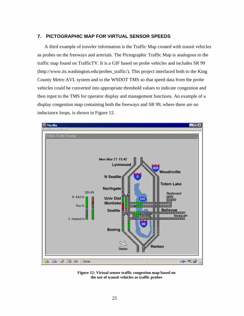
7. PICTOGRAPHIC MAP FOR VIRTUAL SENSOR SPEEDS

A third example of traveler information is the Traffic Map created with transit vehicles

as probes on the freeways and arterials. The Pictographic Traffic Map is analogous to the

traffic map found on TrafficTV. It is a GIF based on probe vehicles and includes SR 99

(http://www.its.washington.edu/probes_traffic/). This project interfaced both to the King

County Metro AVL system and to the WSDOT TMS so that speed data from the probe

vehicles could be converted into appropriate threshold values to indicate congestion and

then input to the TMS for operator display and management functions. An example of a

display congestion map containing both the freeways and SR 99, where there are no

inductance loops, is shown in Figure 12.

Figure 12: Virtual sensor traffic congestion map based on the use of transit vehicles as traffic probes

25

8. CONCLUSIONS

The WSDOT operates a central TMS for both day-to-day surveillance and traveler

information. Past efforts developed the ability to create real-time traffic speed information

by using virtual sensors based on transit vehicle tracking data. In order for this new

information source to be merged into the TMS, a number of questions, such as probe density

in time and space, had to be resolved.

This report presents the solution developed at the University of Washington (UW).

This solution provides real-time congestion information from I-5, I-90, SR 520 and SR 99 to

WSDOT’s TMS by using the ITS Backbone. This project harvests existing AVL data from

within King County Metro Transit and transports the raw data to the UW, where a series of

operations converts the data into roadway speed information. This roadway speed

information is color coded on the basis of specific, localized conditions for the arterials and

freeways to reflect traffic congestion. The resulting traffic data product is then provided to

WSDOT as a data source for virtual sensors located in roadways where currently there are

no inductance loops.

In addition to creating the infrastructure for an AVL-equipped fleet to serve as probe

vehicles, this project created several user interfaces for traveler information. One is

“StoreView,” a Java application that displays the spatial and temporal average speeds of

transit vehicles as bubbles on a map of the major arterials and freeways. The bubbles are

color-coded to reflect local traffic conditions. This application can be found at

http://www.its.washington.edu/storeview/storeview.jnlp.

Another type of traveler information, analogous to TrafficTV and WSDOT’s

pictographic traffic maps, is also available. This interface can be found at

http://www.its.washington.edu/probes_traffic/.

This report documents both the technical issues addressed in creating a virtual sensor

data stream from probe vehicle data and the creation of a set of real-time traveler

information applications.

This work demonstrated the creation of a set of practical real-time virtual sensors

based on probe vehicles. Furthermore, it identified a framework in which an existing transit

fleet can be used as probe vehicles. It created the software to implement this new data source

26

within the existing TMS at WSDOT’s TSMC. WSDOT personnel at TSMC are presently

evaluating the use of probe data to populate a traffic map for Aurora Avenue (SR 99).

27

REFERENCES

1. Elango, C. and D. Dailey. “Irregularly sampled transit vehicles used as a probe

vehicle traffic sensor.” Transportation Research Record1719, pp. 33–44, 2002.

2. Dailey, D.J., and M.P. Haselkorn, K. Guiberson, and P. Lin. Automatic Transit

Location System. Washington State Transportation Center - TRAC/WSDOT, Final

Technical Report WA-RD 394.1, 49 pages, February 1996.

3. Dailey, D. and F. Cathey. “Virtual speed sensors using transit vehicles as traffic

probes.” Proceedings of the IEEE 5th International Conference on Intelligent

Transportation Systems, pp. 560–565, 2002

4. Cathey, F.W. and D.J. Dailey. “Transit Vehicles as Traffic Probe Sensors.”

Transportation Research Record 1804, pp. 23-30, 2002.

5. Bell, B.M. “The Marginal Likelihood for Parameters in a Discrete Gauss-Markov

Process.” IEEE Transactions on Signal Processing, Vol. 48, No. 3, pp. 870-873,

March 2000.

6. Jazwinski, A.H. Stochastic Processes and Filtering Theory. New York, Academic

Press, 1970.

7. Rauch, H.E., F. Tung, and C.T. Striebel. “Maximum Likelihood Estimates of Linear

Dynamic Systems.” American Institute of Aeronautics and Astronautics Journal,

Vol. 3, pp. 1445-1450, August 1965.

8. Anderson, B.D.0. and J.B. Moore. Optimal Filtering. Englewood Cliffs, New Jersey:

Prentice Hall, c1979.

9. Press, W.H., S.A. Teukolsky, W.T. Vetterling, and B.P. Flannery. Numerical Recipes

in C, The Art of Scientific Computing. Cambridge; New York: Cambridge University

Press, 1992.

10. Cathey, F. and D. Dailey. “Estimating corridor travel time by using transit vehicles

as probes.” Transportation Research Record 1855, pp. 60–65, 2003.

11. Dailey, D.J., S. Maclean, F. Cathey, and D. Meyers. “Self describing data transfer

model in intelligent transportation systems applications.” IEEE Transactions on

Intelligent Transportation Systems, Vol. 3, No. 4, pp. 293–300, 2002.

28

12. Dailey, D.J., D. Meyers, and N. Friedland. “A Self Describing Data Transfer

Methodology for ITS Applications.” Transportation Research Record 1660, pp. 140-

147, 1999.

29

30