AUTORREGRESIVE CONDITIONAL VOLATILITY, SKEWNESS AND KURTOSIS

Forthcoming in the Quarterly Journal of Economics and Finance

Ángel León Universidad de Alicante

Dpto. Economía Financiera

Gonzalo Rubio Universidad del País Vasco

Dpto. Fundamentos Análisis Económico II

Gregorio Serna Universidad de Castilla − La Mancha

Dpto. Economía Financiera

December 2004

JEL Clasification: G12, G13, C13, C14 Keywords: Conditional volatility, skewness and kurtosis; Gram-Charlier series expansion; Stock indices. Corresponding author: Ángel León, Dpto. Economía Financiera, Facultad de Ciencia Económicas, Universidad de Alicante, Apartado de Correos 99, 03080 Alicante, Spain; E-mail: aleon@ua.es We have received valuable comments from an anonymous referee, Alfonso Novales, Ignacio Peña and Hipolit Torró. Ángel León and Gonzalo Rubio acknowledge the financial support provided by the Ministerio de Ciencia y Tecnología, grants BEC2002-03797 and BEC2001-0636 respectively, and also thank the Fundación BBVA research grant 1-BBVA 00044.321-15466/2002

-2-

Abstract

This paper proposes a GARCH-type model allowing for time-varying volatility,

skewness and kurtosis. The model is estimated assuming a Gram-Charlier series

expansion of the normal density function for the error term, which is easier to estimate

than the non-central t distribution proposed by Harvey and Siddique (1999). Moreover,

this approach accounts for time-varying skewness and kurtosis while the approach by

Harvey and Siddique (1999) only accounts for nonnormal skewness. We apply this

method to daily returns of a variety of stock indices and exchange rates. Our results

indicate a significant presence of conditional skewness and kurtosis. It is also found that

specifications allowing for time-varying skewness and kurtosis outperform

specifications with constant third and fourth moments.

-3-

AUTORREGRESIVE CONDITIONAL VOLATILITY, SKEWNESS AND KURTOSIS

1. Introduction

There have been many papers studying the departures from normality of asset return

distributions. It is well known that stock return distributions exhibit negative skewness and

excess kurtosis (see, for example, Harvey and Siddique, 1999; Peiró, 1999; and Premaratne

and Bera, 2001). Specifically, excess kurtosis (the fourth moment of the distribution) makes

extreme observations more likely than in the normal case, which means that the market

gives higher probability to extreme observations than in normal distribution. However, the

presence of negative skewness (the third moment of the distribution) has the effect of

accentuating the left-hand side of the distribution. That is, the market gives higher

probability to decreases than increases in asset pricing.

These issues have been widely analyzed in option pricing literature. For example, as

explained by Das and Sundaram (1999), the well known volatility smile and smirk effects

are closely related to the presence of excess kurtosis and negative skewness in the

underlying asset returns distribution.

The generalized autorregresive conditional heteroscedasticity (GARCH) models,

introduced by Engle (1982) and Bollerslev (1986), allow for time-varying volatility (but not

for time-varying skewness or kurtosis). Harvey and Siddique (1999) present a way to

jointly estimate time-varying conditional variance and skewness under a non-central t

distribution for the error term in the mean equation. Their methodology is applied to several

series of stock index returns, and it is found that autorregresive conditional skewness is

significant and that the inclusion of skewness affects the persistence in variance. It is

important to point out that the paper by Harvey and Siddique (1999) allows for time-

varying skewness but still assumes constant kurtosis.

Premaratne and Bera (2001) have suggested capturing asymmetry and excess kurtosis with

the Pearson type IV distribution, which has three parameters that can be interpreted as

-4-

volatility, skewness and kurtosis. This is an approximation to the non-central t distribution

proposed by Pearson and Merrington (1958). However, these authors use time-varying

conditional mean and variance, but maintain constant skewness and kurtosis over time.

Similarly, Jondeau and Rockinger (2000) employ a conditional generalized Student-t

distribution to capture conditional skewness and kurtosis by imposing a time-varying

structure for the two parameters which control the probability mass in the assumed

distribution1. However, these parameters do not follow a GARCH structure for either

skewness or kurtosis.

The purpose of this research is to extend the work by Harvey and Siddique (1999)

assuming a distribution for the error term in the mean equation that accounts for nonnormal

skewness and kurtosis. In particular, we jointly estimate time-varying volatility, skewness

and kurtosis using a Gram-Charlier series expansion of the normal density function, along

the lines suggested by Gallant and Tauchen (1989).

It is also worth noting that, apart from the fact that our approach accounts for time-varying

kurtosis while the one by Harvey and Siddique (1999) does not, our likelihood function,

based on a series expansion of the normal density function, is easier to estimate than the

likelihood function based on the non-central t distribution employed by them.

The joint estimation of time-varying volatility, skewness and kurtosis can be useful in

testing option pricing models that explicitly introduce the third and fourth moments of the

underlying asset return distribution along the lines suggested by Heston (1993), Bates

(1996), and Heston and Nandi (2000). It may also be useful in analyzing the information

content of option-implied coefficients of skewness and kurtosis, extending the papers by

Day and Lewis (1992), Lamoureux and Lastrapes (1993) and Amin and Ng (1997), among

others.

The method proposed in this paper is applied to two different data sets. Firstly, our model is

estimated using daily returns of four exchange rates series: British Pound/USD, Japanese

1 This generalized Student-t distribution is based on Hansen´s (1994) work.

-5-

Yen/USD, German Mark/USD and Swiss Franc/USD. Secondly we apply the method to

five stock indices: S&P500 and NASDAQ100 (U.S.), DAX30 (Germany), IBEX35 (Spain),

and the MEXBOL emerging market index (Mexico). These indices reflect the movements

in their respective national financial markets and are used as underlying assets in several

options and futures contracts.

Our results indicate significant presence of conditional skewness and kurtosis. It is also

found that specifications allowing for time-varying skewness and kurtosis outperform

specifications with constant third and fourth moments.

The rest of the paper is organized as follows. In Section 2 we present our GARCH-type

model for estimating time-varying variance, skewness and kurtosis jointly. Section 3

presents the data and the empirical results regarding the estimation of the model. Section 4

compares the models allowing for time-varying skewness and kurtosis and the standard

models with constant third and fourth moments. Section 5 concludes with a summary and

discussion.

2. A model for conditional volatility, skewness and kurtosis

In this section we extend the model for conditional variance and skewness proposed by

Harvey and Siddique (1999), to account for conditional kurtosis along the lines discussed in

the introduction.

Given a series of asset prices {S0, S1, …, ST}, we define continuously compounded returns

for period t as ( )[ ]1ttt SSln100r −= , t = 1, 2, …, T. Specifically, we present an asset return

model containing either the GARCH(1,1) or NAGARCH (1,1) structure for conditional

variance2 and also a GARCH (1,1) structure for both conditional skewness and kurtosis.

Under the NAGARCH specification for conditional variance, the model is denoted as

2 Due to the well known leverage effect, we have chosen the NAGARCH (1,1) specification for the variance equation proposed by Engle and Ng (1993).

-6-

NAGARCHSK (and GARCHSK when conditional variance is driven by the GARCH (1,1)

model3). It is given by:

( ) ( )

( ) ( )

( )

1t24

1t10t

1t23

1t10t

1t2221

1t31t10t

t1tttt21

t

2ttt1tt

kk

ss

hhh

h,0I ;1,0 ;h

,0 ;rEr

−−

−−

−−−

−

−

++=

++=

+++=

≈≈=

≈+=

δηδδ

γηγγ

ββεββ

εηηε

σεε ε

(1)

where ( )•−1tE denotes the conditional expectation on an information set till period 1t −

denoted as 1tI − . We establish that ( )1 0t tE η− = , ( )21 1t tE η− = , ( )3

1t t tE sη− = and

( )41t t tE kη− = where both ts and tk are driven by a GARCH (1,1) structure. Hence, ts and

tk represent respectively skewness and kurtosis corresponding to the conditional

distribution of the standardized residual 21ttt h−= εη .

Using a Gram-Charlier (GC) series expansion of the normal density function and truncating

at the fourth moment4, we obtain the following density function for the standardized

residuals tη conditional on the information available in 1t − :

( ) ( ) ( ) ( )

( ) ( )

3 4 21

31 3 6 33! 4!

t tt t t t t t t

t t

s kg Iη φ η η η η η

φ η ψ η

−

− = + − + − +

=

(2)

3 Specifically, in the equations below, we obtain the GARCHSK model for 3 0.β =

-7-

where ( )•φ denotes the probability density function (henceforth pdf) corresponding to the

standard normal distribution and ( )•Ψ is the polynomial part of fourth order corresponding

to the expression between brackets in (2). Note that the pdf defined in (2) is not really a

density function because for some parameter values in (1) the density ( )•g might be

negative due to the component ( )•Ψ . Similarly, the integral of ( )•g on ℜ is not equal to

one. We propose a true pdf, denoted as ( )•f , by transforming the density ( )•g according to

the method in Gallant and Tauchen (1989). Specifically, in order to obtain a well defined

density everywhere we square the polynomial part ( )•Ψ , and to insure that the density

integrates to one we divide by the integral of ( )•g over ℜ 5. The resulting pdf written in

abbreviated form is6:

( ) ( ) ( )21 /t t t t tf Iη φ η ψ η− = Γ (3)

where

( )22 31

3! 4!tt

t

ks −Γ = + +

Therefore, after omitting unessential constants, the logarithm of the likelihood function for

one observation corresponding to the conditional distribution 1/ 2t t thε η= , whose pdf is

( )1/ 21t t th f Iη−− , is given by

( )( ) ( )2 21 1ln ln ln2 2t t t t tl h η ψ η= − − + − Γ (4)

As pointed out before, this likelihood function is clearly easier to estimate than the one

based on a non-central t proposed by Harvey and Siddique (1999). In fact, the likelihood

function in (4) is the same as in the standard normal case plus two adjustment terms

accounting for time-varying skewness and kurtosis. Moreover, it is worth noting that the

4 See Jarrow and Rudd (1982) and also Corrado and Su (1996). 5 See the appendix for proof that this nonnegative function is really a density function that integrates to one. 6 An alternative approach under the Gram-Charlier framework is proposed by Jondeau and Rockinger (2001) who also show how constraints on the parameters defining skewness and kurtosis may be implemented to insure that the expansion defines a density. However, their approach does not seem to be feasible in both skewness and kurtosis within the conditional case.

-8-

density function based on a Gram-Charlier series expansion in equation (3) nests the

normal density function (when st = 0 and kt = 3), while the noncentral t does not. Therefore,

the restrictions imposed by the normal density function with respect to the more general

density based on a Gram-Charlier series expansion can be easily tested. Finally, note that

NAGARCHSK nests the GARCH (1,1) specification for the conditional variance when

03 =β in (1). We denote this nested case as the GARCHSK model.

3. Empirical results

3.1 Data and preliminary findings

Our methodology is applied to two different data sets. The first one includes daily returns

of five exchange rates series: British Pound/USD (GBP/USD), Japanese Yen/USD

(JPY/USD), German Mark/USD (GEM/USD) and Swiss Franc/USD (CHF(USD). The

second data set includes five stock indexes: S&P500 and NASDAQ100 (U.S.), DAX30

(Germany), IBEX35 (Spain) and the emerging market index MEXBOL (Mexico).

Our data set includes daily closing prices from January 2, 1990 to May 3, 2002 for the five

exchange rate series, and from January 2, 1990 to July 17, 2003 for all stock index series

except for MEXBOL, which includes data from January 2, 1995 to July 17, 2003. These

closing prices are employed to calculate the corresponding continuously compounded daily

returns, and Table 1 presents some descriptive statistics. Note that all series show

leptokurtosis and there is also evidence of negative skewness except for GBP/USD and

MEXBOL. It is also worth noting that the Mexican emerging market returns (MEXBOL)

show the highest values of unconditional standard deviation, skewness and kurtosis.

Before we estimate our NAGARCHSK model, we analyze the dynamic structure in the

mean equation of (1). Specifically, the ARMA structure that maximizes the Schwarz

Information Criterion (SIC) is selected. All the parameters implied in every model below

are estimated by maximum likelihood assuming that the Gram-Charlier series expansion

distribution given by (3) holds for the error term, and using Bollerslev and Wooldridge

-9-

(1992) robust standard errors7. If we define the SIC as ln(LML) – (q/2)ln(T), where q is the

number of estimated parameters, T is the number of observations, and LML is the value of

the log likelihood function using the q estimated parameters, then the selected model is the

one with the highest SIC. According to SIC, MA(1) and AR(1) models without constant

term yield very similar results8. However, the AR(1) has the advantage of being consistent

with the nonsynchronous contracts of individual stocks which constitute the indices.

Definitively, the dynamic conditional mean structure for every estimation is represented by

an AR(1) model with no constant term.

Table 2 presents the Ljung-Box statistics of order 20, denoted as LB(20), for εt2, εt

3 and εt4,

where εt is the error term in the AR(1) model (with no constant term). The statistic for all

moments is quite large (p-value = 0.000 in all cases). In other words, the significant serial

correlation for εt2, εt

3 and εt4 indicates time-varying volatility, skewness and kurtosis, and it

justifies the estimation of our GARCHSK or NAGARCHSK models defined in (1) with

time-varying volatility, skewness and kurtosis.

3.2 Model estimation with time-varying volatility, skewness and kurtosis

Before presenting the estimation results obtained with both the exchange rates and the stock

indexes series, we summarize the four nested models estimated as follows:

Mean: t1t1t rr εα += − (5-a)

Variance (GARCH): 1t2

21t10t hh −− ++= βεββ (5-b)

Variance (NAGARCH): ( ) 1t2221

1t31t10t hhh −−− +++= ββεββ(5-c)

Skewness: 1t2

31t10t ss −− ++= γεγγ (5-d)

Kurtosis: 1t2

41t10t kk −− ++= δεδδ (5-e)

7 All maximum likelihood estimations in this paper are carried out using the CML subroutine of GAUSS. 8 The constant terms were never significant in previous tests.

-10-

We estimate first two standard models for conditional variance: the GARCH (1,1) model

(equations (5-a) and (5-b)), and the NAGARCH (1,1) model (equations (5-a) and (5-c)),

where a normal distribution is assumed for the unconditional standardized error tη . We

also estimate the generalizations of the standard GARCH and NAGARCH models, with

time-varying skewness and kurtosis, named GARCHSK (equations (5-a), (5-b), (5-d) and

(5-e)) and NAGARCHSK (equations (5-a), (5-c), (5-d) and (5-e)), assuming in both cases

the distribution based on the Gram-Charlier series expansion given by equation (3). In the

NAGARCH specification of the variance equation, a negative value of β3 implies a

negative correlation between shocks and conditional variance.

It should be noted that, given that the likelihood function is highly nonlinear, special care

must be taken in selecting the starting values of the parameters. As usual in these cases,

given that the four models are nested, the estimation is performed following several stages,

and using the parameters estimated from the simpler models as starting values for more

complex ones.

The results for the exchange rate series are presented in Tables 3 and 4 for the GARCH and

GARCHSK models respectively. It is found that for all exchange rates series the coefficient

for asymmetric variance, 3β , is not significant, confirming that the leverage effect,

commonly observed in other financial series, is not observed in the case of exchange rates.

Therefore, for the exchange rate series only the results for symmetric variance models are

presented.

As expected, the results for all exchange rate series indicate a significant presence of

conditional variance. Volatility is found to be persistent since the coefficient of lagged

volatility is positive and significant, indicating that high conditional variance is followed by

high conditional variance.

Moreover, it is found that for the GBP/USD, DEM/USD and CHF/USD exchange rate

series, days with high skewness are followed by days with high skewness, since the

coefficient for lagged skewness ( 2γ ) is positive and significant, although its magnitude is

-11-

lower than in the variance case. Also, shocks to skewness are significant, although they are

less relevant than its persistence. However, there seems to be no structure in skewness in

the JPY/USD series, since neither 1γ nor 2γ is significant in this case.

As with skewness, the results for the kurtosis equation indicate that days with high kurtosis

are followed by days with high kurtosis, since the coefficient for lagged kurtosis ( 2δ ) is

positive and significant. Its magnitude is greater than that of skewness but still lower than

that of variance. As before, shocks to kurtosis are significant, except for the JPY/USD

series.

Finally, it is worth noting that the value of the SIC, shown at the bottom of Tables 3 and 4,

rises monotonically in all cases when we move from the simpler models to the more

complicated ones, with the GARCHSK model showing the highest figure. Therefore, for

the four exchange rates series analyzed, the GARCHSK specification seems to be the most

appropriate one according to the SIC criterion.

The results for the five stock indices are presented in Tables 5, 6, 7 and 8 for GARCH,

NAGARCH, GARCHSK and NAGARCHSK models respectively.

As expected, the results shown in Table 5 (GARCH models) indicate significant presence

of conditional variance, with the two American indices (S&P500 and NASDAQ100)

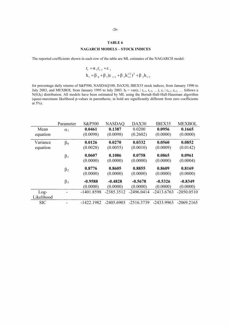
showing the highest degree of persistence. However, Table 6 (NAGARCH models) shows

that contrary to the exchange rate case, the coefficient for asymmetric variance, 3β ,is

negative and significant, confirming the presence of the leverage effect commonly observed

in the markets.

In regard to the skewness equation (Tables 7 and 8), as before, significant presence of

conditional skewness is found, with at least one of the coefficients associated with shocks

to skewness ( 1γ ) and to lagged skewness ( 2γ ) being significant, except for S&P500 stock

index under the NAGARCHSK specification.

-12-

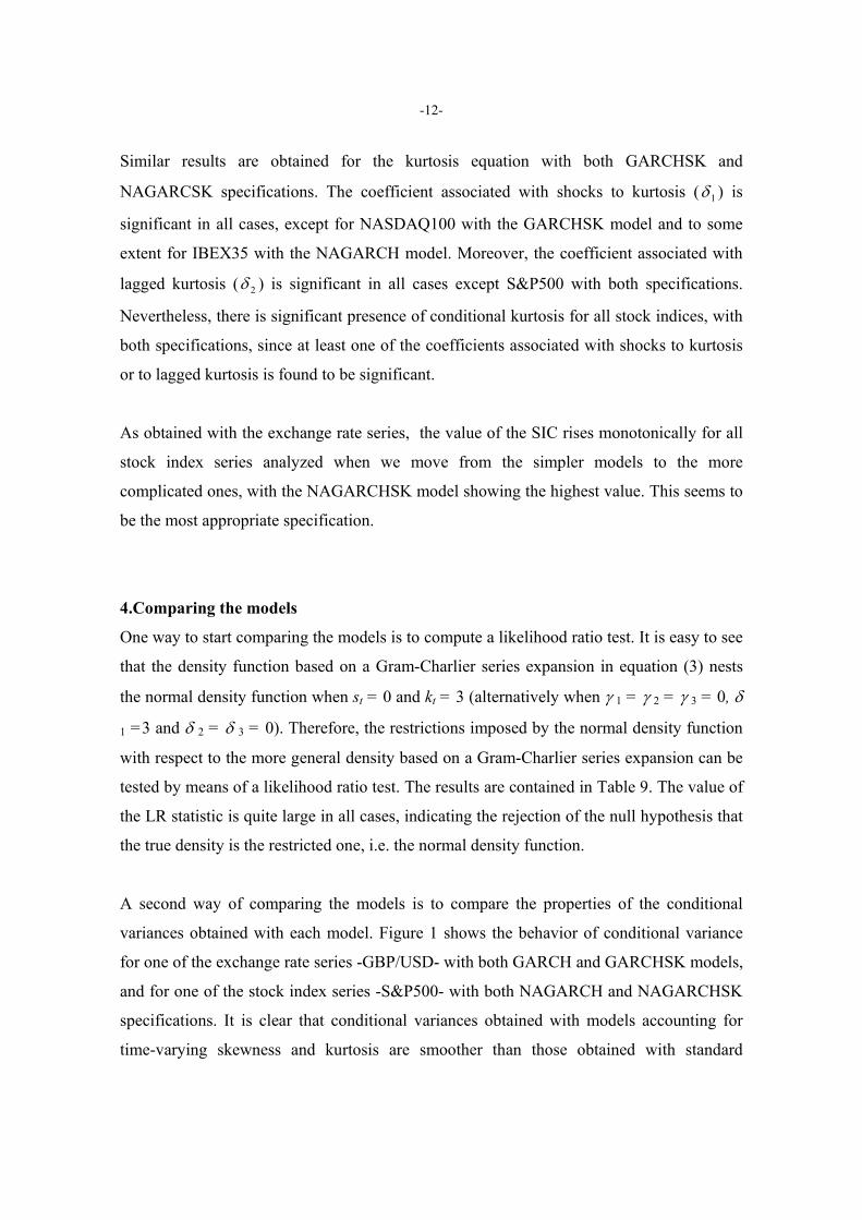
Similar results are obtained for the kurtosis equation with both GARCHSK and

NAGARCSK specifications. The coefficient associated with shocks to kurtosis ( 1δ ) is

significant in all cases, except for NASDAQ100 with the GARCHSK model and to some

extent for IBEX35 with the NAGARCH model. Moreover, the coefficient associated with

lagged kurtosis ( 2δ ) is significant in all cases except S&P500 with both specifications.

Nevertheless, there is significant presence of conditional kurtosis for all stock indices, with

both specifications, since at least one of the coefficients associated with shocks to kurtosis

or to lagged kurtosis is found to be significant.

As obtained with the exchange rate series, the value of the SIC rises monotonically for all

stock index series analyzed when we move from the simpler models to the more

complicated ones, with the NAGARCHSK model showing the highest value. This seems to

be the most appropriate specification.

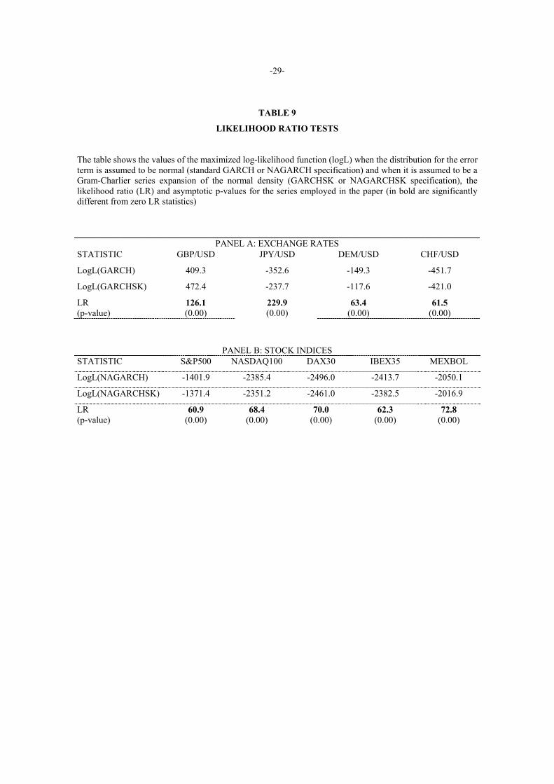
4.Comparing the models

One way to start comparing the models is to compute a likelihood ratio test. It is easy to see

that the density function based on a Gram-Charlier series expansion in equation (3) nests

the normal density function when st = 0 and kt = 3 (alternatively when γ 1 = γ 2 = γ 3 = 0, δ

1 =3 and δ 2 = δ 3 = 0). Therefore, the restrictions imposed by the normal density function

with respect to the more general density based on a Gram-Charlier series expansion can be

tested by means of a likelihood ratio test. The results are contained in Table 9. The value of

the LR statistic is quite large in all cases, indicating the rejection of the null hypothesis that

the true density is the restricted one, i.e. the normal density function.

A second way of comparing the models is to compare the properties of the conditional

variances obtained with each model. Figure 1 shows the behavior of conditional variance

for one of the exchange rate series -GBP/USD- with both GARCH and GARCHSK models,

and for one of the stock index series -S&P500- with both NAGARCH and NAGARCHSK

specifications. It is clear that conditional variances obtained with models accounting for

time-varying skewness and kurtosis are smoother than those obtained with standard

-13-

GARCH or NAGARCH models. This is confirmed by the results in Table 10, which shows

some descriptive statistics for these conditional variances. In fact, conditional variances

obtained with GARCHSK or NAGARCHSK models show less standard deviation,

skewness and kurtosis than those obtained with the standard models. This fact was

observed by Harvey and Siddique (1999) with their time-varying skewness (although

constant-kurtosis) specification.

The in-sample predictive ability of the different models is compared by means of two

metrics. The variable predicted is the squared forecast error (εt2) and the predictors are the

conditional variances (ht) from, respectively, the standard GARCH or NAGARCH models

and GARCHSK or NAGARCHSK models. The two metrics are:

Median absolute error: |)(| 2tt hmedMAE −= ε

Median percentage absolute error:

−= 2

2 ||

t

tt hmedMPAE

εε

The metrics are based on the median since it is more robust than the mean in view of the

high dispersal of the error series. The results are shown in Table 11. Models accounting for

time-varying skewness and kurtosis outperform standard GARCH or NAGARCH models.

They are the best performing models with the two metrics with all exchange rates and stock

index series except for NASDAQ100 and IBEX35 with the median absolute error (although

not with the median percentage absolute error).

Furthermore, it is worth noting that the series that performs best, based on these metrics, is

the MEXBOL stock index, which is the series with the highest values of unconditional

standard deviation, skewness and kurtosis (Table 1). This result could suggest the potential

application of our methodology to financial series from emerging economies, characterized

by higher risk and more pronounced departures from normality.

-14-

5. Conclusions

It is well known that the generalized autorregresive conditional heteroscedasticity

(GARCH) models, introduced by Engle (1982) and Bollerslev (1986) allow for time-

varying volatility (but not for time-varying skewness or kurtosis). However, given the

increasing attention that time-varying skewness and kurtosis have attracted in option

pricing literature, it may be useful to analyze a model that jointly accounts for conditional

second, third and fourth moments.

Harvey and Siddique (1999) present a way of jointly estimating time-varying conditional

variance and skewness, assuming a non-central t distribution for the error term in the mean

equation. We propose a GARCH-type model allowing for time-varying volatility, skewness

and kurtosis. The model is estimated assuming a Gram-Charlier series expansion of the

normal density function, along the lines suggested by Gallant and Tauchen (1989), for the

error term in the mean equation. This distribution is easier to estimate than the non-central t

distribution proposed by Harvey and Siddique (1999). Moreover, our approach accounts for

time-varying skewness and kurtosis while the one by Harvey and Siddique (1999) only

accounts for time-varying skewness.

Firstly, our model is estimated using daily returns of four exchange rate series, five stock

indices and the emerging market index MEXBOL (Mexico). Our results indicate significant

presence of conditional skewness and kurtosis. Moreover, it is found that specifications

allowing for time-varying skewness and kurtosis outperform specifications with constant

third and fourth moments.

Finally, it is important to point out two main implications of our GARCHSK and

NAGARCHSK model. First, they can be useful in estimating future coefficients of

volatility, skewness and kurtosis, which are unknown parameters in option pricing models

that account for nonnormal skewness and kurtosis. For example, estimates of volatility,

skewness and kurtosis from the NAGARCHSK model, based on historical series of returns,

could be compared with option implied coefficients in terms of their out of sample option

pricing performance. Secondly, our models could be useful in testing the information

-15-

content of option implied coefficients of volatility, skewness and kurtosis. This could be

done by including option implied coefficients as exogenous terms in the equations of

volatility, skewness and kurtosis, extending the papers by Day and Lewis (1992),

Lamoureux and Lastrapes (1993) and Amin and Ng (1997), among others.

-16-

APPENDIX Here we show that the nonnegative function ( )1t tf Iη − in (3) is really a density function,

that is it integrates to one. We can rewrite ( )tψ η in (2) as:

( ) ( ) ( )3 431

3! 4!t t

t t ts kH Hψ η η η−

= + +

where ( ){ } Ν∈ii xH represents the Hermite polynomials such that ( ) ( )0 11,H x H x x= = and for 2i ≥ they hold the following recurrence relation:

( ) ( ) ( )( )1 21 /i i iH x xH x i H x i− −= − −

It is verified that ( ){ } Ν∈ii xH is an orthonormal basis satisfying that:

( ) ( ) 1,iH x x dx iφ∞

−∞= ∀∫ (A-1)

( ) ( ) ( ) 0,i jH x H x x dx i jφ∞

−∞= ∀ ≠∫ (A-2)

where ( )•φ denotes the N(0,1) density function. If we integrate the conditional density function in (3), given conditions (A-1) and (A-2):

( ) ( ) ( ) ( )

( ) ( ) ( ) ( ) ( ) ( ) ( )

( ) ( )

2

3 4

222 23 4

22

31/ 13! 4!

31/

3! 4!

31/ 1

3! 4!

1.

t tt t t t t

ttt t t t t t t t t

ttt

s kH H d

ksd H d H d

ks

φ η η η η

φ η η η φ η η η φ η η

∞

−∞

∞ ∞ ∞

−∞ −∞ −∞

− Γ + +

−= Γ + +

−= Γ + +

=

∫

∫ ∫ ∫

-17-

REFERENCES

Amin, K. and V. Ng (1997), “Inferring Future Volatility from the Information in Implied

Volatility in Eurodollar Options: A New Approach”, The Review of Financial Studies 10,

333-367.

Backus, D., Foresi, S., Li, K. and L. Wu (1997), “Accounting for Biases in Black-Scholes”,

Working Paper, Stern School of Business, New York University.

Bates, D. (1996), “Jumps and Stochastic Volatility: Exchange Rate Processes Implicit in

Deutschemark Options”, The Review of Financial Studies 9, 69-107.

Bollerslev, T. (1986), “Generalized Autorregresive Conditional Heteroskedasticity”,

Journal of Econometrics 31, 307-327.

Bollerslev, T. and J. Wooldridge (1992), “Quasi-Maximum Likelihood Estimation and

Inference y Dynamic Models with Time-Varying Covariances”, Econometric Reviews 11,

143-172.

Corrado, C. and T. Su (1996), “Skewness and Kurtosis in S&P 500 index returns implied

by option prices”, Journal of Financial Research 19, 175-192.

Das, S and R. Sundaram (1999), “Of Smiles and Smirks: A Term Structure Perspective”,

Journal of Financial and Quantitative Analysis 34, 211-239.

Day, T. and C. Lewis (1992), “Stock market volatility and the information content of stock

index options”, Journal of Econometrics 52, 267-287.

Engle, R. F. (1982), “Autorregresive Conditional Heteroskedasticity with Estimates of the

Variance of U.K. Inflation”, Econometrica 50, 987-1008.

-18-

Engle, R. F. and V. K. Ng (1993), “Measuring and Testing the Impact of News on

Volatility”, The Journal of Finance 48, 1749-1778.

Gallant, A. R. and G. Tauchen (1989), “Seminonparametric Estimation of Conditionally

Constrained Heterogeneous Processes: Asset Pricing Applications”, Econometrica 57,

1091-1120.

Hansen, B. (1994), “Autorregresive Conditional Density Estimation”, International

Economic Review 35, 705-730.

Harvey, C. R. and A. Siddique (1999), “Autorregresive Conditional Skewness”, Journal of

Financial and Quantitative Analysis 34, 465-487.

Heston, S. (1993), “A Closed-Form Solution for Options with Stochastic Volatility, with

Applications to Bond and Currency Options”, The Review of Financial Studies 6, 327-343.

Heston, S. and S. Nandi (2000), “A Closed-Form GARCH Option Valuation Model”, The

Review of Financial Studies 13, 585-625.

Jarrow, R. and A. Rudd (1982), “Approximate Option Valuation for Arbitrary Stochastic

Processes”, Journal of Financial Economics 10, 347-369.

Jondeau, E. and M. Rockinger (2000), “Conditional Volatility, Skewness and Kurtosis:

Existence and Persistence”, Working Paper, HEC School of Management.

Jondeau, E. and M. Rockinger (2001), “Gram-Charlier Densities”, Journal of Economic

Dynamics & Control 25, 1457-1483.

Lamoureux, C. and W. Lastrapes (1993), “Forecasting Stock-Return Variance: Toward an

Understanding of Stochastic Implied Volatilities”, The Review of Financial Studies 6, 293-

326.

-19-

Pearson, E. S. and M. Merrington (1958), “An approximation to the distribution of

noncentral t”, Biometrica 45, 484-491.

Peiró, A. (1999), “Skewness in financial returns”, Journal of Banking and Finance 23, 847-

862.

Premaratne, G. and A. K. Bera (2001), “Modeling Asymmetry and Excess Kurtosis in

Stock Return Data”, Working Paper, Department of Economics, University of Illinois.

-20-

FIGURE 1 ESTIMATED CONDITIONAL VARIANCES WITH NAGARCH AND NAGARCHSK

MODELS

CONDITONAL VARIANCE

GARCH GBP/USD

CONDITONAL VARIANCE

GARCHSK GBP/USD

CONDITIONAL VARIANCE

NAGARCH S&P500

CONDITIONAL VARIANCE

NAGARCHSK S&P500

0.0

0.2

0.4

0.6

0.8

1.0

1.2

1.4

1.6

500 1000 1500 2000 2500 30000.0

0.2

0.4

0.6

0.8

1.0

1.2

1.4

1.6

500 1000 1500 2000 2500 3000

0

2

4

6

8

10

500 1000 1500 2000 2500 30000

2

4

6

8

10

500 1000 1500 2000 2500 3000

-21-

TABLE 1

DESCRIPTIVE STATISTICS FOR DAILY RETURNS

PANEL A: EXCHANGE RATES

STATISTIC GBP/USD JPY/USD DEM/USD CHF/USD

Simple size 3126 3126 3126 3126

Mean 0.0030 -0.0045 0.0072 0.0003

Median 0.0000 0.0120 0.0207 0.0217

Maximum 3.2860 3.3004 3.1203 3.0747

Minimum -2.8506 -5.7093 -2.9497 -3.7243

Stand. Dev. 0.5731 0.7192 0.6621 0.7197

Skewness 0.2334 -0.5794 -0.0594 -0.2000

Kurtosis 5.7502 7.3298 4.6546 4.5432

Jarque-Bera (p-value)

1013.565 (0.0000)

2616.775 (0.0000)

358.4119 (0.0000)

331.0593 (0.000)

PANEL B: STOCK INDEXES

STATISTIC S&P500 NASDAQ DAX30 IBEX35 MEXBOL

Simple size 3415 3416 3407 3390 2137

Mean 0.0294 0.0383 0.0178 0.0246 0.0511

Median 0.0315 0.1217 0.0641 0.0508 0.0099

Maximum 5.5732 13.2546 7.5527 6.8372 12.1536

Minimum -7.1127 -10.1684 -8.8747 -8.8758 -14.3139

Stand. Dev. 1.0611 1.6117 1.5056 1.3876 1.8086

Skewness -0.0995 -0.0099 -0.1944 -0.1854 0.0712

Kurtosis 6.5658 8.3740 6.3210 5.9169 8.6060

Jarque-Bera (p-value)

1814.880 (0.0000)

4110.566 (0.0000)

1587.134 (0.0000)

1221.204 (0.0000)

2800.124 (0.0000)

-22-

TABLE 2

LJUNG-BOX STATISTICS WITH ORDER 20 OF RESIDUALS FROM AR(1) MODEL

The table presents the Ljung-Box statistic (asymptotic p-value in parenthesis) with order 20, i.e. LB(20), of εt

2, εt3 and εt

4, where εt is the error term from an AR(1) model for daily returns (in bold are significantly different from zero Ljung-Box statistics)

SERIES LB(20) - εt2 LB(20) - εt

3 LB(20) - εt4

GBP/USD 825.43 (0.000)

134.37 (0.000)

332.34 (0.000)

JPY/USD 567.01 (0.000)

208.55 (0.000)

196.37 (0.000)

DEM/USD 407.25 (0.000)

70.501 (0.000)

187.38 (0.000)

CHF/USD 317.69 (0.000)

133.75 (0.000)

365.89 (0.000)

S&P500 131.81 (0.000)

120.91 (0.000)

139.79 (0.000)

NASDAQ 3152.1 (0.000)

252.04 (0.000)

315.26 (0.000)

DAX30 2919.1 (0.000)

72.889 (0.000)

489.37 (0.000)

IBEX35 1719.1 (0.000)

131.16 (0.000)

271.49 (0.000)

MEXBOL 488.67 (0.000)

238.18 (0.000)

283.82 (0.000)

-23-

TABLE 3

GARCH MODELS – EXCHANGE RATES

The reported coefficients shown in each row of the table are ML estimates of the standard GARCH model:

t1t1t εrαr += −

1t22

1t10t hβεββh −− ++= for percentage daily returns of British Pound/American Dollar (GBP/USD), Japanese Yen/US Dollar (JPY/USD), German Mark/US Dollar (DEM/USD) and Swiss Franc/US Dollar (CHF/USD) exchange rates, from January 1990 to March 2002. ht = var(rt | rt-1, rt-2, …), εt | εt-1, εt-2, … follows a N(0,ht) distribution. All models have been estimated by ML using the Berndt-Hall-Hall-Hausman algorithm (quasi-maximum likelihood p-values in parenthesis; in bold are significantly different from zero coefficients at 5%).

Parameter GBP/USD JPY/USD DEM/USD CHF/USD Mean

equation α1 0.0432

(0.0263) 0.0175

(0.3826) 0.0364

(0.0573) 0.0304

(0.1154)

Variance equation

β0

β1

β2

0.0031 (0.0459)

0.0435 (0.0000)

0.9468 (0.0000)

0.0086 (0.0645)

0.0428 (0.0011)

0.9402 0.0000)

0.0051 (0.0663)

0.0378 (0.0000)

0.9502 (0.0000)

0.0111 (0.0715)

0.0336 (0.0003)

0.94445 (0.0000)

Log-Likelihood

- 409.3328 -352.5956 -149.3089 -451.7276

SIC - 393.2391 -368.6843 -165.4027 -467.8213

-24-

TABLE 4 GARCHSK MODELS – EXCHANGE RATES

The reported coefficients shown in each row of the table are ML estimates of the GARCHSK model:

t1t1t εrαr += −

1t22

1t10t hβεββh −− ++=

1t24

1t10t

1t23

1t10t

kδηδδk

s γη γγs

−−

−−

++=

++=

for percentage daily returns of of Brithis Pound/US Dollar (GBP/USD), Japanese Yen/US Dollar (JPY/USD), German Mark/US Dollar (DEM/USD) and Swiss Franc/US Dollar (CHF/USD) exchange rates, from January 1990 to March 2002. ht = var(rt | rt-1, rt-2, …), st = skewness(rt | rt-1, rt-2, …), kt = kurtosis(rt | rt-1, rt-2, …), ηt = εt ht

-1/2, and εt | εt-1, εt-2, … follows the distribution based on a Gram-Charlier series expansion. All models have been estimated by ML using the Berndt-Hall-Hall-Hausman algorithm (quasi-maximum likelihood p-values in parenthesis; in bold are significantly different from zero coefficients at 5%).

Parameter GBP/USD JPY/USD DEM/USD CHF/USD Mean

equation α1 0.0219

(0.2537) -0.0030 (0.8670)

0.0249 (0.3804)

0.0015 (0.9322)

Variance equation

β0

β1

β2

0.0015 (0.0783)

0.0366 (0.0000)

0.9550 (0.0000)

0.0061 (0.0378)

0.0309 (0.0021)

0.9537 (0.0000)

0.0022 (0.0159)

0.0236 (0.0000)

0.9690 (0.0000)

0.0075 (0.0007)

0.0217 (0.0000)

0.9611 (0.0000)

Skewness equation

γ0

γ1

γ2

0.0053 (0.5379)

0.0093 (0.0004)

0.6180 (0.0000)

-0.0494 (0.0482)

0.0018 (0.4190)

0.3414 (0.2097)

-0.0270 (0.0398)

0.0175 (0.0054)

0.4421 (0.0000)

-0.0242 (0.0989)

0.0054 (0.0688)

0.6468 (0.0002)

Kurtosis equation

δ0

δ1

δ2

1.3023 (0.0000)

0.0028 (0.0000)

0.6229 (0.0000)

1.2365 (0.0038)

0.0014 (0.1102)

0.6464 (0.0000)

1.9649 (0.0000)

0.01356 (0.0000)

0.4045 (0.0002)

0.5500 (0.0000)

0.0060 (0.0000)

0.8303 (0.0000)

Log-Likelihood

- 472.3652 -237.6668 -117.5896 -420.9973

SIC - 432.1309 -277.9012 -157.8240 -461.2317

-25-

TABLE 5

GARCH MODELS - STOCK INDICES

The reported coefficients shown in each row of the table are ML estimates of the standard GARCH model:

t1t1t εrαr += −

1t22

1t10t hβεββh −− ++= for percentage daily returns of S&P500, NASDAQ100, DAX30, IBEX35 stock indices, from January 1990 to July 2003, and MEXBOL from January 1995 to July 2003. ht = var(rt | rt-1, rt-2, …), εt | εt-1, εt-2, … follows a N(0,ht) distribution. All models have been estimated by ML using the Berndt-Hall-Hall-Hausman algorithm (quasi-maximum likelihood p-values in parenthesis; in bold are significantly different from zero coefficients at 5%).

Parameter S&P500 NASDAQ DAX30 IBEX35 MEXBOL Mean

equation α1 0.03394

(0.0544) 0.1266

(0.0000) 0.0179

(0.3133) 0.0943

(0.0000) 0.1564

(0.0000)

Variance equation

β0

β1

β2

0.0055 (0.0414)

0.0587 (0.0000)

0.9379 (0.0000)

0.0149 (0.0155)

0.0948 (0.0000)

0.9009 (0.0000)

0.0317 (0.0092)

0.09394 (0.0000)

0.8918 (0.0000)

0.05741 (0.0026)

0.1035 (0.0000)

0.8666 (0.0000)

0.0827 (0.0958)

0.1194 (0.0098)

0.8591 (0.0000)

Log-Likelihood

- -1459.6826 -2424.1550 -2525.9824 -2441.0090 -2095.6885

SIC - -1475.9532 -2440.4262 -2542.2484 -2457.2650 -2111.0210

-26-

TABLE 6

NAGARCH MODELS – STOCK INDICES

The reported coefficients shown in each row of the table are ML estimates of the NAGARCH model:

t1t1t εrαr += −

1t221/2

1-t31t10t hβ)hβε(ββh −− +++= for percentage daily returns of S&P500, NASDAQ100, DAX30, IBEX35 stock indices, from January 1990 to July 2003, and MEXBOL from January 1995 to July 2003. ht = var(rt | rt-1, rt-2, …), εt | εt-1, εt-2, … follows a N(0,ht) distribution. All models have been estimated by ML using the Berndt-Hall-Hall-Hausman algorithm (quasi-maximum likelihood p-values in parenthesis; in bold are significantly different from zero coefficients at 5%).

Parameter S&P500 NASDAQ DAX30 IBEX35 MEXBOL Mean

equation α1 0.0461

(0.0098) 0.1387

(0.0098) 0.0200

(0.2602) 0.0956

(0.0000) 0.1665

(0.0000)

Variance equation

β0

β1

β2

β3

0.0126 (0.0028)

0.0607 (0.0000)

0.8776 (0.0000)

-0.9588 (0.0000)

0.0270 (0.0055)

0.1086 (0.0000)

0.8605 (0.0000)

-0.4828 (0.0000)

0.0332 (0.0010)

0.0758 (0.0000)

0.8855 (0.0000)

-0.5678 (0.0000)

0.0560 (0.0009)

0.0865 (0.0000)

0.8609 (0.0000)

-0.5326 (0.0000)

0.0852 (0.0142)

0.0961 (0.0004)

0.8169 (0.0000)

-0.8349 (0.0000)

Log-Likelihood

- -1401.8598 -2385.3512 -2496.0414 -2413.6763 -2050.0510

SIC - -1422.1982 -2405.6903 -2516.3739 -2433.9963 -2069.2165

-27-

TABLE 7 GARCHSK MODELS – STOCK INDICES

The reported coefficients shown in each row of the table are ML estimates of the GARCHSK model:

t1t1t εrαr += −

1t22

1t10t hβεββh −− ++=

1t24

1t10t

1t23

1t10t

kδηδδk

s γη γγs

−−

−−

++=

++=

for percentage daily returns of S&P500, NASDAQ100, DAX30, IBEX35 stock indices, from January 1990 to July 2003, and MEXBOL from January 1995 to July 2003. ht = var(rt | rt-1, rt-2, …), st = skewness(rt | rt-1, rt-2, …), kt = kurtosis(rt | rt-1, rt-2, …), ηt = εt ht

-1/2, and εt | εt-1, εt-2, … follows the distribution based on a Gram-Charlier series expansion. All models have been estimated by ML using the Berndt-Hall-Hall-Hausman algorithm (quasi-maximum likelihood p-values in parenthesis; in bold are significantly different from zero coefficients at 5%).

Parameter S&P500 NASDAQ DAX30 IBEX35 MEXBOL Mean

equation α1 0.0211

(0.2285) 0.1229

(0.0000) 0.0080

(0.6557) 0.0949

(0.0000) 0.1775

(0.0000)

Variance equation

β0

β1

β2

0.0023 (0.1117)

0.0387 (0.0000)

0.9586 (0.0000)

0.0098 (0.0202)

0.0822 (0.0000)

0.9149 (0.0000)

0.0261 (0.0119)

0.0851 (0.0000)

0.9021 (0.0000)

0.0417 (0.0042)

0.0843 (0.0000)

0.8928 (0.0000)

0.1228 (0.0028)

0.1663 (0.0000)

0.8023 (0.0000)

Skewness equation

γ0

γ1

γ2

-0.0458 (0.0518)

0.0085 (0.0139)

0.0227 (0.9187)

-0.0886 (0.0106)

0.0078 (0.0032)

0.2174 (0.4136)

-0.0245 (0.2911)

0.0048 (0.2006)

0.6781 (0.0168)

-0.0446 (0.0161)

0.0189 (0.0000)

0.1352 (0.0852)

0.0228 (0.3101)

0.0125 (0.0136)

0.2969 (0.3112)

Kurtosis equation

δ0

δ1

δ2

3.0471 (0.0000)

0.0055 (0.0019)

0.0882 (0.5715)

1.4576 (0.0175)

0.0007 (0.6228)

0.5518 (0.0034)

0.4866 (0.0016)

0.0010 (0.0229)

0.8493 (0.0000)

0.2526 (0.0026)

0.0004 (0.0129)

0.9208 (0.0000)

0.3302 (0.0254)

0.0010 (0.3634)

0.9018 (0.0000)

Log-Likelihood

- -1404.5752 -2375.0218 -2484.1335 -2414.6928 -2056.0966

SIC - -1445.2519 -2415.7000 -2525.7985 -2455.3328 -2094.4277

-28-

TABLE 8 NAGARCHSK MODELS – STOCK INDICES

The reported coefficients shown in each row of the table are ML estimates of the NAGARCHSK model:

t1t1t εrαr += −

1t221/2

1-t31t10t hβ)hβε(ββh −− +++=

1t24

1t10t

1t23

1t10t

kδηδδk

s γη γγs

−−

−−

++=

++=

for percentage daily returns of S&P500, NASDAQ100, DAX30, IBEX35 stock indices, from January 1990 to July 2003, and MEXBOL from January 1995 to July 2003. ht = var(rt | rt-1, rt-2, …), st = skewness(rt | rt-1, rt-2, …), kt = kurtosis(rt | rt-1, rt-2, …), ηt = εt ht

-1/2, and εt | εt-1, εt-2, … follows the distribution based on a Gram-Charlier series expansion. All models have been estimated by ML using the Berndt-Hall-Hall-Hausman algorithm (quasi-maximum likelihood p-values in parenthesis; in bold are significantly different from zero coefficients).

Parameter S&P500 NASDAQ DAX30 IBEX35 MEXBOL Mean

equation α1 0.0358

(0.0466) 0.1255

(0.0000) 0.0152

(0.4009) 0.1024

(0.0000) 0.1742

(0.0000)

Variance equation

β0

β1

β2

β3

0.0083 (0.0006)

0.0416 (0.0000)

0.9099 (0.0373)

-1.0116 (0.0000)

0.01841 (0.0038)

0.0986 (0.0000)

0.8801 (0.0000)

-0.4351 (0.0000)

0.0278 (0.0005)

0.0696 (0.0000)

0.8961 (0.0000)

-0.5597 (0.0000)

0.04460 (0.0004)

0.0729 (0.0000)

0.8800 (0.0000)

-0.5795 (0.0003)

0.1000 (0.0001)

0.1202 (0.0000)

0.7834 (0.0000)

-0.7703 (0.0000)

Skewness equation

γ0

γ1

γ2

-0.0451 (0.0373)

0.0091 (0.1034)

0.0552 (0.7418)

-0.0618 (0.0005)

0.0103 (0.0025)

0.4572 (0.0000)

-0.0261 (0.2285)

0.0050 (0.1883)

0.6573 (0.0124)

-0.0204 (0.1174)

0.0045 (0.1423)

0.5325 (0.0022)

0.0525 (0.0782)

0.0180 (0.0045)

0.1922 (0.5459)

Kurtosis equation

δ0

δ1

δ2

3.1652 (0.0000)

0.0150 (0.0000)

0.0293 (0.6645)

1.6929 (0.0003)

0.0053 (0.0025)

0.4684 (0.0014)

0.4536 (0.0016)

0.0009 (0.0161)

0.8581 (0.0000)

0.2012 (0.0858)

0.0004 (0.0749)

0.9365 (0.0000)

1.9901 (0.0011)

0.0055 (0.0004)

0.4017 (0.0271)

Log-Likelihood

- -1371.4169 -2351.1665 -2461.0251 -2382.5437 -2016.8569

SIC - -1416.1613 -2395.9126 -2505.7566 -2427.2477 -2059.0212

-29-

TABLE 9

LIKELIHOOD RATIO TESTS

The table shows the values of the maximized log-likelihood function (logL) when the distribution for the error term is assumed to be normal (standard GARCH or NAGARCH specification) and when it is assumed to be a Gram-Charlier series expansion of the normal density (GARCHSK or NAGARCHSK specification), the likelihood ratio (LR) and asymptotic p-values for the series employed in the paper (in bold are significantly different from zero LR statistics)

PANEL A: EXCHANGE RATES STATISTIC GBP/USD JPY/USD DEM/USD CHF/USD

LogL(GARCH) 409.3 -352.6 -149.3 -451.7

LogL(GARCHSK) 472.4 -237.7 -117.6 -421.0

LR (p-value)

126.1 (0.00)

229.9 (0.00)

63.4 (0.00)

61.5 (0.00)

PANEL B: STOCK INDICES STATISTIC S&P500 NASDAQ100 DAX30 IBEX35 MEXBOL

LogL(NAGARCH) -1401.9 -2385.4 -2496.0 -2413.7 -2050.1

LogL(NAGARCHSK) -1371.4 -2351.2 -2461.0 -2382.5 -2016.9

LR (p-value)

60.9 (0.00)

68.4 (0.00)

70.0 (0.00)

62.3 (0.00)

72.8 (0.00)

-30-

TABLE 10

DESCRIPTIVE STATISTICS FOR CONDITIONAL VARIANCES

The table shows the main descriptive statistics for the conditional variances obtained from GARCH and GARCHSK models for GBP/USD series, and from NAGARCH and NAGARCHSK models for S&P500 series paper (in bold are significantly different from zero Jarque-Bera statistics)

GBP/USD S&P500

STATISTIC ht - GARCH ht – GARCHSK ht - NAGARCH ht - NAGARCHSK

Simple size 3124 3124 3413 3413

Mean 0.3264 0.3026 1.1394 1.0928

Median 0.2647 0.2432 0.7692 0.7513

Maximum 1.4762 1.3944 8.3534 6.9340

Minimum 0.0988 0.0776 0.1731 0.1771

Stand. Dev. 0.2034 0.1980 1.0575 0.9533

Skewness 2.2384 2.1624 2.5160 2.2077

Kurtosis 9.4659 8.9007 11.1431 8.9475

Jarque-Bera (p-value)

8050.721 (0.0000)

6966.893 (0.0000)

13030.790 (0.0000)

7802.598 (0.0000)

-31-

TABLE 11

IN-SAMPLE PREDICTIVE POWER

The variable predicted is the squared forecast error (εt2) and the predictors are the conditional variances (ht)

from, respectively, the standard GARCH or NAGARCH models and GARCHSK or NAGARCHSK models. Two metrics are chosen to compare the predictive power ability of these models:

1. Median absolute error |)(| 2tt hmedMAE −= ε

2. Median percentage absolute error

−= 2

2 ||

t

tt hmedMPAE

εε

The metrics are based on the median given the high dispersion of the error series.

SERIES MAE MPAE G 0.2030 1.9227 GBP/USD GSK 0.1874 1.6567 G 0.3369 2.2226 JPY/USD GSK 0.3165 2.0134 G 0.3058 1.7982 DEM/USD GSK 0.2895 1.6028 G 0.3749 1.8096 CHF/USD GSK 0.3635 1.6788 NG 0.5884 1.7690 S&P500 NGSK 0.5723 1.7670 NG 0.9061 1.3801 NASDAQ NGSK 0.9209 1.3075 NG 1.0225 1.5102 DAX30 NGSK 1.0207 1.5071 NG 1.0081 1.4610 IBEX35 NGSK 1.0109 1.4349 NG 1.6743 1.6508 MEXBOL NGSK 1.6308 1.5531