automotive data acquisition system - fst - técnico … data acquisition system - fst david rua...
TRANSCRIPT
Automotive data acquisition system - FST
David Rua Copetonº 53598
Dissertation for obtaining the Master’s Degree in
Electrical and Computer Engineering
Jury
President: Prof. Marcelino SantosAdvisor: Prof. Francisco AlegriaCo-Advisor: Prof. Moisés PiedadeSpecialist: Prof. Nuno Roma
October 2009

ii

Resumo
Esta tese aborda o design, a implementação e a validação de um sistema de telemetria para umprotótipo Formula Student, tendo em mente uma rede de sensores suportada num barramento CAN,existente neste. Para o conseguir, o sistema proposto é dividido em dois blocos: uma estação móvele uma estação base. A primeira, é colocada no veículo e ligada aos seus sensores através do barra-mento CAN. Esta estação móvel tem a função de gravar localmente os dados gerados pela actividadeno barramento e também de transferir sem fios, estes dados, para a estação base fora da pista. Asegunda, tem a função de pegar nos dados recebidos através do canal sem-fios e de os apresentarao utilizador de uma forma atraente e compreensível. Para além do funcionamento “online”, a estaçãobase também permite a apresentação de dados relativos a sessões anteriores para análise.
Dado o tipo de veículo (e competição) a que este trabalho se aplica, existem algumas exigênciastanto em termos de capacidade do sistema, como de gestão do projecto. Por um lado, o sistema deveser capaz de resistir a ambientes adversos, nomeadamente vibração, calor, líquidos e interferênciaelectromagnética, e por outro deve ser leve, barato e fácil de utilizar.
O sistema de telemetria desenvolvido foi utilizado com sucesso numa pista de treinos, sendo capazde gravar com fiabilidade os dados provenientes do barramento CAN com um número, frequência deamostragem e tipo variável de sensores. A performance do canal de rádio entre estações foi tambémobtida, tanto num ambiente controlado como real, de maneira a perceber quais os limites do sistema.Os resultados mostram uma taxa de transferência de dados sem-fios de 4.28 kB/s para uma localiza-ção típica do veículo em pista.
Palavras chave: Telemetria, barramento CAN, Zigbee, Formula Student, gravação de dados emambiente automóvel, interface gráfica do utilizador.
iii

iv

Abstract
This thesis addresses the design, implementation and validation of a telemetry system for a FormulaStudent prototype vehicle, having in mind an existing CAN-bus network of sensors in it. To achieve this,the proposed system is divided in two blocks: a mobile station and a base station. The first, is placedon the vehicle and is connected to its sensors through a CAN-bus. This mobile station has the functionof recording locally the data generated by the bus activity and also of transferring this data wirelesslyto the base station located off-track. The second has the function of picking up the data sent throughthe wireless link and presenting it in an attractive and comprehensible way to the user. Besides the“online” operation, the base station is also capable of presenting data from previous logging sessionsfor analysis.
Given the type of vehicle (and competition) this work is applied to, certain requirements are set interms of both system capabilities and project management. In one hand the system must be able tosustain a harsh environment, namely vibration, heat, liquids and electromagnetic interference, and onthe other hand it must be lightweight, cheap and user-friendly.
The developed telemetry system was successfully deployed on a practice track, being able to reli-ably record CAN-bus data of a variable number, sample rate and type of sensors. The performance ofthe radio link between stations was also evaluated both in controlled and real environments in order tounderstand the limits of the system. The results show a maximum wireless data rate of 4.28 kB/s for atypical vehicle position on track.
Keywords: Telemetry, CAN-bus, Zigbee, Formula Student, automotive data logger, graphical userinterface.
v

vi

Contents
Resumo iii
Abstract v
Contents vii
List of Tables ix
List of Figures xi
List of Abbreviations xvii
1 Introduction 11.1 Project scope and objective . . . . . . . . . . . . . . . . . . . . . . . . . . . . . . . . . . . 21.2 State of the art . . . . . . . . . . . . . . . . . . . . . . . . . . . . . . . . . . . . . . . . . . 31.3 System definition . . . . . . . . . . . . . . . . . . . . . . . . . . . . . . . . . . . . . . . . . 41.4 Structure of the thesis . . . . . . . . . . . . . . . . . . . . . . . . . . . . . . . . . . . . . . 5
2 Mobile Station 72.1 Overview . . . . . . . . . . . . . . . . . . . . . . . . . . . . . . . . . . . . . . . . . . . . . 72.2 Microcontroller and Real-Time Clock . . . . . . . . . . . . . . . . . . . . . . . . . . . . . . 8
2.2.1 Microcontroller . . . . . . . . . . . . . . . . . . . . . . . . . . . . . . . . . . . . . . 82.2.2 Real-Time Clock . . . . . . . . . . . . . . . . . . . . . . . . . . . . . . . . . . . . . 9
2.3 CAN-bus Interface . . . . . . . . . . . . . . . . . . . . . . . . . . . . . . . . . . . . . . . . 102.3.1 Protocol . . . . . . . . . . . . . . . . . . . . . . . . . . . . . . . . . . . . . . . . . . 102.3.2 Transceiver and configuration . . . . . . . . . . . . . . . . . . . . . . . . . . . . . . 10
2.4 Wireless Link . . . . . . . . . . . . . . . . . . . . . . . . . . . . . . . . . . . . . . . . . . . 122.4.1 Hardware choice . . . . . . . . . . . . . . . . . . . . . . . . . . . . . . . . . . . . . 122.4.2 Xbee-PRO Zigbee Radios . . . . . . . . . . . . . . . . . . . . . . . . . . . . . . . . 132.4.3 Connection to the microcontroller and configuration . . . . . . . . . . . . . . . . . 20
2.5 Data storage . . . . . . . . . . . . . . . . . . . . . . . . . . . . . . . . . . . . . . . . . . . 222.5.1 Hardware choice . . . . . . . . . . . . . . . . . . . . . . . . . . . . . . . . . . . . . 222.5.2 Vinculum USB Host Controller . . . . . . . . . . . . . . . . . . . . . . . . . . . . . 22
2.6 Power supply . . . . . . . . . . . . . . . . . . . . . . . . . . . . . . . . . . . . . . . . . . . 252.6.1 Voltage level sources . . . . . . . . . . . . . . . . . . . . . . . . . . . . . . . . . . 252.6.2 Power consumption . . . . . . . . . . . . . . . . . . . . . . . . . . . . . . . . . . . 25
2.7 Prototype construction . . . . . . . . . . . . . . . . . . . . . . . . . . . . . . . . . . . . . . 27
vii

2.7.1 Printed Circuit Board layout . . . . . . . . . . . . . . . . . . . . . . . . . . . . . . . 27
2.7.2 Enclosure . . . . . . . . . . . . . . . . . . . . . . . . . . . . . . . . . . . . . . . . . 27
2.8 Software . . . . . . . . . . . . . . . . . . . . . . . . . . . . . . . . . . . . . . . . . . . . . . 30
2.8.1 Overview . . . . . . . . . . . . . . . . . . . . . . . . . . . . . . . . . . . . . . . . . 30
2.8.2 Main function . . . . . . . . . . . . . . . . . . . . . . . . . . . . . . . . . . . . . . . 31
2.8.3 Real-Time Clock setup and access routines . . . . . . . . . . . . . . . . . . . . . . 31
2.8.4 Data storage routines . . . . . . . . . . . . . . . . . . . . . . . . . . . . . . . . . . 32
2.8.5 Xbee-PRO/Serial interruption execution . . . . . . . . . . . . . . . . . . . . . . . . 33
2.8.6 CAN-bus interruption execution . . . . . . . . . . . . . . . . . . . . . . . . . . . . . 33
2.8.7 Message format and feedback command set . . . . . . . . . . . . . . . . . . . . . 34
3 Base Station 37
3.1 Overview . . . . . . . . . . . . . . . . . . . . . . . . . . . . . . . . . . . . . . . . . . . . . 37
3.2 Programming language choice . . . . . . . . . . . . . . . . . . . . . . . . . . . . . . . . . 38
3.3 Software . . . . . . . . . . . . . . . . . . . . . . . . . . . . . . . . . . . . . . . . . . . . . . 39
3.3.1 Objective . . . . . . . . . . . . . . . . . . . . . . . . . . . . . . . . . . . . . . . . . 39
3.3.2 Structure . . . . . . . . . . . . . . . . . . . . . . . . . . . . . . . . . . . . . . . . . 39
3.3.3 Functionality details . . . . . . . . . . . . . . . . . . . . . . . . . . . . . . . . . . . 39
4 System performance 47
4.1 Bench tests . . . . . . . . . . . . . . . . . . . . . . . . . . . . . . . . . . . . . . . . . . . . 47
4.1.1 CAN-bus network emulation platform . . . . . . . . . . . . . . . . . . . . . . . . . . 47
4.1.2 CAN-bus interruption routine timming . . . . . . . . . . . . . . . . . . . . . . . . . 49
4.1.3 Wireless link maximum throughput . . . . . . . . . . . . . . . . . . . . . . . . . . . 50
4.2 Track tests . . . . . . . . . . . . . . . . . . . . . . . . . . . . . . . . . . . . . . . . . . . . . 51
4.2.1 Performance for different base station positioning . . . . . . . . . . . . . . . . . . . 52
4.2.2 Wireless link maximum throughput . . . . . . . . . . . . . . . . . . . . . . . . . . . 55
4.2.3 Considerations on mechanical behaviour . . . . . . . . . . . . . . . . . . . . . . . 56
5 Conclusions 57
5.1 Future work . . . . . . . . . . . . . . . . . . . . . . . . . . . . . . . . . . . . . . . . . . . . 58
5.2 Cost analysis . . . . . . . . . . . . . . . . . . . . . . . . . . . . . . . . . . . . . . . . . . . 58
Bibliography 60
Appendix A - Formula Student and Projecto FST 63
A.1 Formula Student . . . . . . . . . . . . . . . . . . . . . . . . . . . . . . . . . . . . . . . . . 63
A.2 Projecto FST . . . . . . . . . . . . . . . . . . . . . . . . . . . . . . . . . . . . . . . . . . . 64
Appendix B - CAN-bus protocol 65
B.1 Message arbitration . . . . . . . . . . . . . . . . . . . . . . . . . . . . . . . . . . . . . . . 65
B.2 Error handling . . . . . . . . . . . . . . . . . . . . . . . . . . . . . . . . . . . . . . . . . . . 65
B.3 Message format . . . . . . . . . . . . . . . . . . . . . . . . . . . . . . . . . . . . . . . . . 66
B.4 Bit timming . . . . . . . . . . . . . . . . . . . . . . . . . . . . . . . . . . . . . . . . . . . . 66
viii

Appendix C - Circuit diagrams of the mobile station board 69C.1 Microcontroller . . . . . . . . . . . . . . . . . . . . . . . . . . . . . . . . . . . . . . . . . . 69C.2 Real-Time Clock . . . . . . . . . . . . . . . . . . . . . . . . . . . . . . . . . . . . . . . . . 70C.3 CAN-bus transceiver . . . . . . . . . . . . . . . . . . . . . . . . . . . . . . . . . . . . . . . 70C.4 Wireless transceiver . . . . . . . . . . . . . . . . . . . . . . . . . . . . . . . . . . . . . . . 71C.5 USB host controller . . . . . . . . . . . . . . . . . . . . . . . . . . . . . . . . . . . . . . . . 71C.6 Power Supply . . . . . . . . . . . . . . . . . . . . . . . . . . . . . . . . . . . . . . . . . . . 72
Appendix D - Radio link 73D.1 X-CTU software . . . . . . . . . . . . . . . . . . . . . . . . . . . . . . . . . . . . . . . . . 73D.2 Tranceivers comparison chart . . . . . . . . . . . . . . . . . . . . . . . . . . . . . . . . . . 74
Appendix E - Flow diagrams of the mobile station’s software 75E.1 Real-Time Clock setup and access routines . . . . . . . . . . . . . . . . . . . . . . . . . . 75E.2 Main function . . . . . . . . . . . . . . . . . . . . . . . . . . . . . . . . . . . . . . . . . . . 76E.3 Data storage routines . . . . . . . . . . . . . . . . . . . . . . . . . . . . . . . . . . . . . . 77E.4 Xbee-PRO/Serial interruption execution . . . . . . . . . . . . . . . . . . . . . . . . . . . . 82E.5 CAN-bus interruption execution . . . . . . . . . . . . . . . . . . . . . . . . . . . . . . . . . 83
Appendix F - Layout of the mobile station’s board 85
Appendix G - Base station’s software 89G.1 Class diagram . . . . . . . . . . . . . . . . . . . . . . . . . . . . . . . . . . . . . . . . . . 89G.2 File examples . . . . . . . . . . . . . . . . . . . . . . . . . . . . . . . . . . . . . . . . . . . 90
ix

x

List of Tables
2.1 Bit timming registers setting for 1 Mbit/s CAN-bus operation. . . . . . . . . . . . . . . . . . 112.2 Transceivers’ details chart. . . . . . . . . . . . . . . . . . . . . . . . . . . . . . . . . . . . 132.3 XBee-PRO transceivers specifications. . . . . . . . . . . . . . . . . . . . . . . . . . . . . . 142.4 Jumper setting for port selection. . . . . . . . . . . . . . . . . . . . . . . . . . . . . . . . . 242.5 User information LEDs’ behaviour. . . . . . . . . . . . . . . . . . . . . . . . . . . . . . . . 292.6 Vinculum’s functions by interaction type. . . . . . . . . . . . . . . . . . . . . . . . . . . . . 322.7 Actions triggered by the serial line interrupt routine. . . . . . . . . . . . . . . . . . . . . . . 332.8 Set of feedback frames used by the mobile station. . . . . . . . . . . . . . . . . . . . . . . 35
5.1 Prototype cost’s breakdown. . . . . . . . . . . . . . . . . . . . . . . . . . . . . . . . . . . . 595.2 Total cost of the system for 3 different cases. . . . . . . . . . . . . . . . . . . . . . . . . . 59
A.1 Technical specifications of FST03. . . . . . . . . . . . . . . . . . . . . . . . . . . . . . . . 64
C.1 VDIP1 data and configuration pins for each bus interface. . . . . . . . . . . . . . . . . . . 72
D.1 XBee-PRO configuration options in X-CTU. . . . . . . . . . . . . . . . . . . . . . . . . . . 73D.2 Transceivers’ details chart. . . . . . . . . . . . . . . . . . . . . . . . . . . . . . . . . . . . 74
F.1 Altium Designer layout details. . . . . . . . . . . . . . . . . . . . . . . . . . . . . . . . . . 85
xi

xii

List of Figures
1.1 General outline of a digital data logging system. . . . . . . . . . . . . . . . . . . . . . . . . 11.2 The prototype FST03 during a test run. . . . . . . . . . . . . . . . . . . . . . . . . . . . . 21.3 The main building blocks of the system . . . . . . . . . . . . . . . . . . . . . . . . . . . . . 4
2.1 The mobile station’s board with all its components . . . . . . . . . . . . . . . . . . . . . . 72.2 Microcontroller PIC18F4685 connections block diagram. . . . . . . . . . . . . . . . . . . . 82.3 Real-Time clock DS3232 connections block diagram. . . . . . . . . . . . . . . . . . . . . . 92.4 CAN-bus transceiver MCP2551 connections block diagram. . . . . . . . . . . . . . . . . . 102.5 CAN-bus physical layer block diagram. . . . . . . . . . . . . . . . . . . . . . . . . . . . . . 112.6 Google Earth image of KIP, the practice track used. . . . . . . . . . . . . . . . . . . . . . . 122.7 XBee-PRO transceivers fitted with a whip antenna and a male U.FL antenna connector. . 132.8 Setup for spectral analysis of RF transceivers. . . . . . . . . . . . . . . . . . . . . . . . . . 142.9 XBee-PRO radio sitting on the development board . . . . . . . . . . . . . . . . . . . . . . 152.10 Center frequency measurement for 18 dBm (60 mW) power output setting. . . . . . . . . 162.11 Channel power measurement for 18 dBm (60 mW) power output setting. . . . . . . . . . . 162.12 Occupied bandwidth measurement for 18 dBm (60 mW) power output setting. . . . . . . . 172.13 ACPR measurement for 18 dBm (60 mW) power output setting. . . . . . . . . . . . . . . . 182.14 Setup for the longer distance test at a beach. . . . . . . . . . . . . . . . . . . . . . . . . . 182.15 Results of the measurements taken at the IST Alameda university campus . . . . . . . . 192.16 Results of the measurements taken at a beach . . . . . . . . . . . . . . . . . . . . . . . . 202.17 Zigbee transceiver XBee-PRO connections block diagram. . . . . . . . . . . . . . . . . . 202.18 Microcontroller and USB drive seamless integration through Vinculum. . . . . . . . . . . . 232.19 The VDIP1 development module that includes the Vinculum IC. . . . . . . . . . . . . . . . 232.20 VDIP1 module schematic detail. . . . . . . . . . . . . . . . . . . . . . . . . . . . . . . . . 242.21 Power supply block diagram. . . . . . . . . . . . . . . . . . . . . . . . . . . . . . . . . . . 252.22 Setup used for the mobile station’s current consuption measurement. . . . . . . . . . . . 262.23 Osciloscope image of a current burst that happens during transmission of a through the
wireless link. . . . . . . . . . . . . . . . . . . . . . . . . . . . . . . . . . . . . . . . . . . . 262.24 Produced mobile station’s board prototype. . . . . . . . . . . . . . . . . . . . . . . . . . . 272.25 Final assembly of the PCB board inside the enclosure fitted with cables to the connector
and power switch. The transceiver adapting cable and the main regulator heatsink canalso be seen. . . . . . . . . . . . . . . . . . . . . . . . . . . . . . . . . . . . . . . . . . . . 28
2.26 Mobile station’s enclosure sticker. . . . . . . . . . . . . . . . . . . . . . . . . . . . . . . . . 282.27 Final mobile station’s prototype. . . . . . . . . . . . . . . . . . . . . . . . . . . . . . . . . . 292.28 State diagram of the mobile station software. . . . . . . . . . . . . . . . . . . . . . . . . . 302.29 Format of the messages sent from the mobile station. . . . . . . . . . . . . . . . . . . . . 34
xiii

3.1 Base station. . . . . . . . . . . . . . . . . . . . . . . . . . . . . . . . . . . . . . . . . . . . 373.2 General structure of the base station software. . . . . . . . . . . . . . . . . . . . . . . . . 403.3 Wizard start page. . . . . . . . . . . . . . . . . . . . . . . . . . . . . . . . . . . . . . . . . 413.4 Name and previous session reading in a new Online session. . . . . . . . . . . . . . . . . 423.5 Configuration of the CAN-bus network structure in a new Online session. . . . . . . . . . 423.6 Finding a previous session file (Offline session). . . . . . . . . . . . . . . . . . . . . . . . 433.7 Adding the type information when data is read from the USB memory’s file (Offline session). 433.8 Main window in an Online session. . . . . . . . . . . . . . . . . . . . . . . . . . . . . . . . 443.9 The 8 sensor display widgets. (a) Engine RPM, (b) Wheel speed, (c) Suspension dis-
placement, (d) Tire temperature, (e) Steering position, (f) Sine Wave, (g) Engine coolanttemperature, (h) Throttle position. . . . . . . . . . . . . . . . . . . . . . . . . . . . . . . . . 44
3.10 The two constant components of the Online session main window. . . . . . . . . . . . . . 453.11 Main window in an Offline session. . . . . . . . . . . . . . . . . . . . . . . . . . . . . . . . 46
4.1 Block diagram of the CAN-bus network emulation platform. . . . . . . . . . . . . . . . . . 484.2 CAN-bus network emulation platform built. . . . . . . . . . . . . . . . . . . . . . . . . . . . 484.3 Results of the measurements of vinculumWriteToFile() and sendFrame() function calls’
time. . . . . . . . . . . . . . . . . . . . . . . . . . . . . . . . . . . . . . . . . . . . . . . . . 494.4 Setup for the maximum throughput measurement on the bench. . . . . . . . . . . . . . . . 504.5 Results of the measurements of the wireless link throughput in the bench. Expected
value in red and the system’s value in blue. . . . . . . . . . . . . . . . . . . . . . . . . . . 514.6 Sensors network on the vehicle. The nodes (green) are connected to the mobile station
(red) through the CAN-bus (yellow). Sensors: tire temperature (orange), wheel speed(blue), suspension displacement (dark red), throttle (yellow), engine RPM (red), enginecoolant temperature (pink) and steering angle (gray). . . . . . . . . . . . . . . . . . . . . . 52
4.7 Practice track image with points of interest. Location 1 (blue square), Location 2 (redsquare), Track point 1 (green circle), Track point 2 (yellow circle), Trees (green elipse)and Low area (orange elipse). . . . . . . . . . . . . . . . . . . . . . . . . . . . . . . . . . . 53
4.8 Example of a sine wave with short imperfections (black circle). . . . . . . . . . . . . . . . 544.9 Data acquired at the practice track. Temperatures of the tire’s inside (pink) and outside
(red), the throttle’s position (blue) and the engine’s RPM (green). . . . . . . . . . . . . . . 544.10 Results of the measurements of the wireless link throughput in the track. Expected value
in blue and the system’s value in green. . . . . . . . . . . . . . . . . . . . . . . . . . . . . 554.11 Mobile station installation on the vehicle using zip ties for secure hold. . . . . . . . . . . . 56
B.1 CAN 2.0B data frame. . . . . . . . . . . . . . . . . . . . . . . . . . . . . . . . . . . . . . . 66B.2 A CAN bit and its segments. . . . . . . . . . . . . . . . . . . . . . . . . . . . . . . . . . . . 66
C.1 Schematic diagram of the PIC18F4685. . . . . . . . . . . . . . . . . . . . . . . . . . . . . 69C.2 Schematic diagram of the DS3232. . . . . . . . . . . . . . . . . . . . . . . . . . . . . . . . 70C.3 Schematic diagram of the MCP2551. . . . . . . . . . . . . . . . . . . . . . . . . . . . . . . 70C.4 Schematic diagram of the XBee-PRO. . . . . . . . . . . . . . . . . . . . . . . . . . . . . . 71C.5 Schematic diagram of the VDIP. . . . . . . . . . . . . . . . . . . . . . . . . . . . . . . . . . 71C.6 Schematic diagram of the voltage regulators that power the system. . . . . . . . . . . . . 72
E.1 Flowchart of the setTime() function. . . . . . . . . . . . . . . . . . . . . . . . . . . . . . . 75
xiv

E.2 Flowchart of the readTime() function. . . . . . . . . . . . . . . . . . . . . . . . . . . . . . . 75E.3 Flowchart of the main() function. . . . . . . . . . . . . . . . . . . . . . . . . . . . . . . . . 76E.4 Flowchart of the vinculumInit() function. . . . . . . . . . . . . . . . . . . . . . . . . . . . . 77E.5 Flowchart of the vinculumDriveStart() function. . . . . . . . . . . . . . . . . . . . . . . . . 77E.6 Flowchart of the vinculumDriveStart2() function. . . . . . . . . . . . . . . . . . . . . . . . 78E.7 Flowchart of the vinculumWaitDrive() function. . . . . . . . . . . . . . . . . . . . . . . . . 78E.8 Flowchart of the vinculumOpenFile() function. . . . . . . . . . . . . . . . . . . . . . . . . . 79E.9 Flowchart of the vinculumWriteFilePreamble() function. . . . . . . . . . . . . . . . . . . . 80E.10 Flowchart of the vinculumWriteFile() function. . . . . . . . . . . . . . . . . . . . . . . . . . 80E.11 Flowchart of the vinculumWriteBlank() function. . . . . . . . . . . . . . . . . . . . . . . . . 81E.12 Flowchart of the vinculumWriteFileEnd() function. . . . . . . . . . . . . . . . . . . . . . . . 81E.13 Flowchart of the vinculumCloseFile() function. . . . . . . . . . . . . . . . . . . . . . . . . . 82E.14 Flowchart of the isrSerial() function. . . . . . . . . . . . . . . . . . . . . . . . . . . . . . . 82E.15 Flowchart of the isrCanrx1() function. . . . . . . . . . . . . . . . . . . . . . . . . . . . . . . 83E.16 Flowchart of the sendFrame() function. . . . . . . . . . . . . . . . . . . . . . . . . . . . . . 83
F.1 Top layer of mobile station’s board. . . . . . . . . . . . . . . . . . . . . . . . . . . . . . . . 86F.2 Bottom layer of mobile station’s board. . . . . . . . . . . . . . . . . . . . . . . . . . . . . . 86F.3 3D image of the mobile station’s board with components in place. . . . . . . . . . . . . . . 87
G.1 Class diagram for the base staion’s software. . . . . . . . . . . . . . . . . . . . . . . . . . 89
xv

xvi

List of Abbreviations
ACPR Adjacent Channel Power Ratio
ASCII American Standard Code for Information Interchange
BCD Binary-coded Decimal
CAN Controller Area Network
CF Compact Flash
COTS Commercial Off-The-Shelf
CPU Central Processing Unit
CRC Cyclic redundancy check
CSMA/CD Carrier Sense Multiple Access/Collision Detection
EEPROM Electrically-Erasable Programmable Read-Only Memory
EMI Electromagnetic Interference
FAT File Allocation Table
FIFO First In, First Out
FSPL Free Space Path Loss
FTDI Future Technology Devices International
GPS Global Positioning System
GSM Global System for Mobile Communications
GUI Graphical User Interface
I²C Inter-Integrated Circuit
IC Integrated Circuit
IMechE Institution of Mechanical Engineers
ISM Industrial, Scientific and Medic
ISO International Standards Organization
IST Instituto Superior Técnico
xvii

KIP Kartódromo Internacional de Palmela
LED Light-Emitting Diode
MCU Microcontroller Unit
MMC Multimedia Card
OS Operating System
PC Personal Computer
PCB Printed Circuit Board
PDIP Plastic Dual-in-line Package
PIC Peripheral Interface Controller
PLL Phase-Locked Loop
RF Radio Frequency
RPM Revolutions Per Minute
RSS Received Signal Strength
RTC Real-Time Clock
SAE Society of Automotive Engineers
SD Secure Digital
SMA SubMiniature version A
SMD Surface Mount Device
SNR Signal to Noise Ratio
TCP Transmission Control Protocol
TCXO Temperature-compensated Crystal Oscillator
TTL Transistor-Transistor Logic
UHF Ultra High Frequency
USART Universal Synchronous Asynchronous Receiver/Transmitter
USB Universal Serial Bus
VDI Verein Deutscher Ingenieure
xviii

Chapter 1
Introduction
A great deal of time, effort and expense goes into the construction of a prototype. It is usually theproduct of the work of a large group of people and represents the tangible result of the breakthroughsaccomplished after many hours of research. It is of major importance then, to have the best enlighten-ment possible on it’s performance and maintenance conditions. With this purpose in mind, it’s easy tounderstand why nowadays sensor networks and their data gathering systems are a mandatory part ofany fairly complex machine. Besides being vital in terms of behavior evaluation, this additional invest-ment is the base on which great cost and time savings can be generated.
Commonly referred to as data loggers, the devices that sample real world phenomenons and storedata that can be manipulated by a computer, range from commercial airliner’s airborne recorders toportable heart rate monitors. Data acquisition and logging systems can have many different purposesand capabilities, but the main building blocks remain the same:
Figure 1.1: General outline of a digital data logging system.
An important field where data loggers have been used extensively is the automotive area. Speciallyin competition, data logging plays an important role, allowing a much easier tuning of vehicles, monitor-ing of critical parts (such as the engine) and as a useful tool for assessing driver performance. Currentsolutions found on the market offer already a great number of options in terms of number of channels,acquisition rates and bus interfaces, suitable for different kinds of competitions and vehicles. The mostcommon features found in Commercial off-the-shelf (COTS) data loggers aimed at competion vehiclesare the ability to record wheel speed, temperature, pressure, engine revolutions per minute (RPM) andpedal travel. More complete systems may also include suspension travel or acceleration in different axis.
Working together with data logging with the objective of quicker access to data, telemetry is nowa-
1

days an increasingly wanted feature. By adding wireless transmission hardware to a data logger, gath-ered data can be analyzed right after being generated, and even in real-time, allowing actions to betaken much quicker. In certain applications, where prototypes may be destroyed (e.g. space explorationsystems), the usage of telemetry is the only way to recover performance data. In competition vehicles,telemetry is typically used to monitor operational parameters and alert for dangerous or failure situa-tions; in case of two-way communication it may also be used to adjust some parameters.
1.1 Project scope and objective
This work is primarily aimed at a particular prototype vehicle (figure 1.2), built at Instituto SuperiorTécnico (IST), to participate in the Formula Student competitions1. These competions, organized by theSociety of Automotive Engineers (SAE) and other engineers societies (IMechE2, VDI3, others), are heldevery year in different countries, not as part of a world championship, but as individual events, each onewith its own character and challenges. In these events, teams of students compete with their prototypesin many different ways, from the dynamic performance of the vehicles on track to the way they managetheir team. More information about Formula Student and the team from IST - Projecto FST, can befound in appendix A.
Figure 1.2: The prototype FST03 during a test run.
Developing the system for a Formula Student prototype, sets certain requirements in terms of bothsystem capabilities and project management. In one hand the system must be able to sustain a harshenvironment, namely vibration, heat, liquids and electromagnetic interference, and on the other hand itmust be lightweight, cheap and user-friendly.
1The competions held worldwide are here generally called Formula Student. The correct name should be Formula SAE® Se-ries
2Institution of Mechanical Engineers - The British engineering society3Verein Deutscher Ingenieure - The Association of German Engineers
2

The project presented here has the objective of designing and building a fully working CAN-bus datalogger with telemetry capabilities for a Formula student prototype vehicle. The system should be ableto connect with an existing CAN-bus network of sensors and assure the recording of all the data put onthe CAN-bus. Besides this, it should be able to transmit live sensor data through a radio link while thevehicle is running on the track to a location off-track, and making it available for the user in an atractiveway. Finally, the built system should be validated in a real environment, that is, working in the prototypevehicle its meant for (figure 1.2).
In the following section the current comercial solutions for the logging of CAN-bus data and com-petion vehicle telemetry are presented and discussed.
1.2 State of the art
The current range of products found on the market with the purpose of logging sensor data in avehicle usually offer the data acquisition module separated from the radio module. Recording directlyfrom sensor inputs to a flash memory, the DL1 from Race Technology [21] is a standard in the dataloggers range. This system goes a bit further by integrating accelerometers in the system as well as ahigh acuracy GPS receiver. This kind of stand-alone data loggers can be found in major manufacturersof race vehicle’s instrumentation and have the advantage of a pretty straight forward implementation.They are also built having in mind a strong integration with a driver display console, thus in order tomake the recorded data available, it has to be downloaded from the memory card.
To be able to implement telemetry from the vehicle, radio modules are found separated from the dataacquisition systems. Coswort [2] (former Pi Technology ) offers a radio system, for data transmissionfrom vehicle to pits, working in the 458 to 468 MHz band at 1 Watt and with a data rate of aproximately16.5 kbps. A low throuput rate if the type of data loggers this system is supposed to work with areconsidered (the Pi Sigma Elite Junior data logger has 16 analog and 8 digital inputs). The functioningof these systems rely on the frequency at which data is sent through the radio link or even on thedetection of proximity between radio stations by signal strength, in order to decide when to transmitdata.
Manufacturers start now to increasingly offer telemetry links relying on WLAN technology (WiFi802.11b/g working on the 2.4 GHz frequency band), because it offers much higher data rates (11or 54 Mbps) - Stack ’s [17] MFR-W and Cosworth’s Pi Ethernet Hub wireless version. Although thethroughput is an undeniable advantage, these systems cannot match the range of lower frequencybands’ technologies that are necessary in certain situations (the full coverage of a Formula 1 race trackpresents a challenge due to the amount of obstructions).
For the logging of CAN-bus messages various solutions for USB interface are found in the market,Kvaser ’s [12] Leaf Light or LAWICEL’s [13] CANUSB, and some manufacturers make available stand-alone CAN-bus recorders that have specially in mind the industrial use of the CAN-bus, like Kvaser ’sline of CAN-bus data loggers (Memorator line).
Also industrial but on a different segment, Telemotive’s [1] Blue piraT, is aimed at automotive testingby logging most buses used in automotive industry - MOST, CAN, LIN and FlexRay.
The only product found in the market, joining CAN-bus and wireless transmission, is Kvaser ’s Black-Bird SemiPro. This device is aimed at testing, and evaluation of networks in situations where mobility is
3

a concern.
In this project, the system developed makes a combination not found on the market of two technolo-gies, the CAN-bus and a Zigbee wireless link that will be discussed further ahead in section 2.4.
1.3 System definition
The proposed system comprises two main blocks: a Mobile station and a Base station. The first, isplaced on the vehicle and is connected to its sensors through a CAN-bus, a vehicle bus protocol usedwidely in the automotive and industrial environments. This mobile station has the function of recordinglocally the data generated in the sensor modules (available through the CAN-bus) and also of transfer-ring this data wirelessly to the base station located off-track. The second has the function of picking upthe data sent through the wireless link and presenting it in an attractive and comprehensible way to theuser. Besides the “online” operation, the base station is also capable of presenting data from previouslogging sessions for analysis. A block diagram of the complete system is shown in figure 1.3.
Figure 1.3: The main building blocks of the system and their connection to the vehicle’s sensor network.
4

1.4 Structure of the thesis
This report is divided in four chapters.In chapter 2 the Mobile station segment of the system is described along with its components,
construction and functioning details. It is explained how data available on a CAN-bus is recorded andsent through a wireless link.
In chapter 3 the Base station segment of the system is presented and it is explained how live datais shown to the user. Further options, in terms of data visualization, in the user interface are alsoexplained.
In chapter 4 the performance of the built system is evaluated in two different environments andconclusions based on system usage are drawn.
In chapter 5 conclusions about the CAN-bus logging and telemetry system are made along with acost analysis and ideas for future improvements.
5

6

Chapter 2
Mobile Station
2.1 Overview
The mobile station is the part of the system that is placed on the vehicle. It has a CAN-bus inter-face, to communicate with the existing sensor network (figure 2.1c), a memory unit to store the data(figure 2.1d), a wireless interface to enable the communication with the base station (figure 2.1e) anda control and processing module to manage its operation (figure 2.1a). Other pieces that compose thesystem are a real-time clock (figure 2.1b) and the power supply regulation (figure 2.1f)
Figure 2.1: The mobile station’s board with all its components. (a) Microcontroller, (b) Real-time clock,(c) CAN-bus transceiver, (d) USB host controller module to connect USB drives, (e) Zigbee radiotransceiver and (f) Power supply regulation.
7

2.2 Microcontroller and Real-Time Clock
2.2.1 Microcontroller
At the core of the mobile station a microcontroller is used to interconnect and control all the othermodules (figure 2.1). The device used is a Microchip’s PIC18F4685 8 bit microcontroller. The use ofa PIC microcontroller in face of other types (AVR, MSP430, etc) is related to the author’s previous ex-perience with this kind of devices. The key features for the choice of this device (among others in itsfamily) are the combination of its large program memory of 96 kB and the peripheral communicationbuses supported - CAN, I²C and USART1 [11].
The fact that this Integrated Circuit (IC) is available both in PDIP and in SMD packages was of anenormous value to the development of this work. The first because it allows a very quick and effortlessdesign to prototype phase, enabling the development to be done first in breadboard without the needto go right away to PCB layout and the second because it allows a very small footprint on the finishedboard, which is of great importance in such an embarked system.
Considering the block diagram in figure 2.2, the microcontroller is the device that interconnects allthe other modules of the Mobile station subsystem. The Microcontroller Unit (MCU) operates at 5 V andruns with an oscillator frequency of 40 MHz, provided by the external 10 MHz crystal in combinationwith the internal 4×PLL. Further details concerning the electrical connections of the microcontroller anda schematic diagram can be found in appendix C.1.
As for the remaining components that can be seen in figure 2.2, the CAN-bus and the radio transceiversused will be described in section 2.3 and section 2.4 respectively, the use of a USB host controller willbe explained in section 2.5 and the RTC will be introduced in the following paragraph.
Figure 2.2: Microcontroller PIC18F4685 connections block diagram.
1Throughout this report the terms Serial line or port are used to refer to the USART communications channel.
8

2.2.2 Real-Time Clock
In order to have a time base for the files created on the memory module (section 2.5) a real-timeclock (RTC) is added to the mobile subsystem (figure 2.1b). Connected to the microcontroller, using anI²C bus, is a Maxim’s DS3232 RTC, which has an accuracy of ±2 ppm and incorporates in its packagean oscillator2, a temperature sensor and age compensating logic, achieving in this way a very robustdevice that can withstand temperature swings [18].
This device’s typical operating voltage should be 3.3 V, but for simplicity of design (level conversionsin its bus lines) it is ran at 5 V, which is still well within its maximum ratings3 [18, page 2].
The DS3232 integrates a battery backup input for continuous timekeeping. A 3 V (200 mAh) coincell battery (CR2032) is connected to it (figure 2.3). When the supply voltage drops bellow the battery’svoltage, the power supply changes to battery mode. In this mode the typical current consumption fortimekeeping is 1.5 µA and therefor the cell’s life is more than 15 years, which is large enough for thisapplication.
Connection to the microcontroller through I²C bus
As mentioned above, an I²C bus enables the communication between the RTC and the microcon-troller (figure 2.3). This is a bi-directional bus that has a Serial Clock Line (SCL) and a Serial Data Line(SDA), with both lines being pulled high by 10 kΩ resistors so that when the bus is free both lines areat the high logic level. All the devices are connected in parallel and each slave device has a uniqueaddress which the master uniquely chooses to communicate with. Although it is a multimaster protocol,only one master can be present at any time since the master node is the device that issues the clockon the SCL line.
For this project, the I²C bus master is always the microcontroller, and the bus working speed is setto Fast Mode, that is, at a maximum 400 kHz clock rate. Details on the RTC’s wiring and connectionwith the MCU can be found in appendix C.2.
Figure 2.3: Real-Time clock DS3232 connections block diagram.
2More precisely it is a temperature-compensated crystal oscillator (TCXO)3Many hours of flawless operation have proven these ratings to be correct
9

2.3 CAN-bus Interface
2.3.1 Protocol
The Controller Area Network (CAN) is a serial communications protocol developed by Bosch [3]widely used in automotive applications. The CAN communication protocol is a Carrier Sense MultipleAccess/Collision Detection (CSMA/CD) protocol. This means that every node on the network mustmonitor the bus for a period of no activity before trying to send a message on the bus (Carrier Sense).Also, once this period of no activity occurs, every node on the bus has an equal opportunity to transmit amessage (Multiple Access). As for the Colision Detection, if two nodes on the network start transmittingat the same time, the nodes will detect the collision and take the appropriate action. In the CAN protocol,a non destructive bitwise arbitration method is utilized, which means that messages will remain intactafter arbitration, even if collisions are detected. All this arbitration takes place without corruption or delayof the higher priority message (the node transmitting the highest priority message will continue and theothers will wait) [9]. More details on the CAN protocol arbitration can be found in appendix B.1.
Another important characteristic of this protocol is that it is a broadcast or message-based type ofprotocol, which means that all the nodes receive all the messages (in opposition to an address-basedtype of protocol), and for specific node addressing to be accomplished, local message filtering must beused [12]. This means that uppon receiving a message, each node decides if the message is kept forfurther processing or immediatly discarded. The protocol guarantees that messages are accepted byeither all nodes or non of them, implementing, for this, several mechanisms to ensure data consistency,error handling and error confinement as is further described in appendix B.2.
2.3.2 Transceiver and configuration
The CAN protocol specification by Bosch does not define the physical layer to be used, so to imple-ment this bus the standard used is the ISO-11898-24. This standard is used for high-speed applications,and it specifies a 5 V differential electrical bus as the physical interface.
In order to interface the CAN-bus controller inside the MCU to the physical medium (figure 2.4), atransceiver is used - Microchip’s MCP2551 CAN transceiver (the schematic diagram of this connectioncan be found in appendix C.3). This IC translates the TTL level signals output by the microcontrollerinto signals conforming to ISO-11898 up to a speed of 1 Mbit/s [10].
Figure 2.4: CAN-bus transceiver MCP2551 connections block diagram.
For the successful CAN-bus operation all the controllers attached to it must be configured to operateat the same speed and so the symbol timing must be the same, although the clock at which each con-troller is working can be different. In the case of the CAN-bus (interconnecting all the sensor modules)
4Defined by the International Standards Organization (ISO) and SAE.
10

this system connects to, the speed is set to 1 Mbit/s, the highest speed the protocol can support. Bysetting the symbol timing registers according to the values in table 2.1 the CAN-bus controller inside theMCU can listen to all the messages on the bus. The way to compute these values and their meaningin terms of bit segments is presented in appendix B.4. The CAN protocol version used in this work is2.0B, but only standard 11 bit identifier are used in the messages. The CAN-bus message format canbe found in appendix B.3.
Table 2.1: Bit timming registers setting for 1 Mbit/s CAN-bus operation.
Register name Value
Synchronization Segment 1Propagation Time Segment 2Phase Buffer Segment 1 4Phase Buffer Segment 2 3Synchronization Jump Width 0Baud Rate Prescaler 1
According to physical layer specification ISO-11898-2 the CAN-bus should be fitted with a terminat-ing resistor of 120 Ω on both ends with the purpose of eliminating signal reflections and ensure the bushas the correct DC values [12], as can be seen in figure 2.5.
Figure 2.5: CAN-bus physical layer block diagram.
11

2.4 Wireless Link
2.4.1 Hardware choice
To implement the wireless communication between the mobile and the base station, different tech-nologies were compared. A common starting point to all the solutions taken into account is the usage ofa Commercial off-the-shelf (COTS) product, an approach justified by the project scope, time constrainand the quality of products found nowadays. In this comparison the requisites taken into account area minimum range of 500 meters and a transmission rate over 80 kbit/s5 and the lowest price possi-ble. The minimum range was set by the distance (plus a margin) the radio must be able to cover both incompetion environment and in the practice track - Kartódromo Internacional de Palmela (KIP) (Fig. 2.6),with the last one being the larger, and therefore the constrain.
Figure 2.6: Google Earth image of KIP, the practice track used.
The choice is between the following 6 wireless technologies: Wi-Fi (IEEE 802.11) [4], Bluetooth(IEEE 802.15.1) [6], WiMAX (IEEE 802.16) [5] [20], GSM, UHF radio and ZigBee (IEEE 802.15.4) [7].The usage of Bluetooth and Wi-Fi modules is set aside because of the shortage of products for a rangehigher than 200 meters, although the transmission rates are high (11 or 54 Mbit/s with Wi-Fi and 1or 3 Mbit/s with Bluetooth). Both WiMAX and GSM are eliminated based on the cost of the solutionsfound, the first due to the very high price of modules (although the transmission rate is high - 75 Mbit/s)and the second due to the pricing over the communications themselves since it uses frequency chan-
5The transmission rate minimum value is based on an estimate amount of data produced by 30 sensors, with a resolution of16 bit, a sampling rate of 100 Hz and considering that this amount is only 60% of the total.
12

nels allocated to mobile communications. The UHF radio devices have much lower transmission rates(115.2 kb/s) although prices and ranges available are very competitive. The ZigBee radios found onthe market present higher transmission rates (250 kbit/s) but have a lower range when compared to theUHF radios. The ZigBee modules taken in consideration have the best transmission rate/price ratio anda range than confortably meets specifications. In table 2.2 a wireless transceivers comparison chartcan be found (or appendix D.2 for an extended version).
Table 2.2: Transceivers’ details chart.
Name Frequency (MHz) TX/RX (kb/s) Power (mW) Price (e)
SparkFun LN96 915 9.6 500 68.76Rfsolutions X8200 900 115.2 500 563.58Rfsolutions 232C-868F 868 38.4 5 143.24Rfsolutions TinyOne Pro 868 38.4 500 113.5Maxstream XTend OEM 900 115.2 1000 138.76Maxstream XTend Modem 900 115.2 1000 231.78Maxstream XBee-PRO OEM 2400 115.2 60 27.91Maxstream XBee-PRO Modem 2400 250 60 84Aerocomm AC4424-200 OEM 2400 576 200 98Aerocomm AC4790-1000 OEM 900 76.8 1000 77.5
2.4.2 Xbee-PRO Zigbee Radios
The chosen modules are MaxStream’s XBee-Pro OEM, that can be seen in figure 2.7. Originallymeant for use in wireless sensor networks due to their low power consumption and low price, thesemodules, operating in the ISM 2.4 GHz frequency band, provide a good solution for reliable commu-nication between the mobile and the base station. The key features of the devices, as given by themanufacturer [19, page 5], are presented in table 2.36.
Figure 2.7: XBee-PRO transceivers fitted with a whip antenna and a male U.FL antenna connector.
6The RF Data Rate value is the total transmission rate off the wireless link (therefore includes payload and packet overhead)and the Serial Interface Data Rate is the transmission rate of the module’s interface.
13

Table 2.3: XBee-PRO transceivers specifications.
Specifications XBee-PRO
Indoor/Urban Range Up to 100 mOutdoor line-of-sight Range Up to 1500 mTransmit Power Output (software selectable) 60 mW (18 dBm) conductedRF Data Rate 250.000 bpsSerial Interface Data Rate (software selectable) 1200-115200 bpsReceiver Sensitivity -100 dBm (1% packet error rate)Supply Voltage 2.8-3.4 VTransmit Current (typical) 215 mA (@ 3.3 V and 18 dBm output power)Idle / Receive Current (typical) 55 mA (@ 3.3 V)Power-down Current < 10 µAOperating Frequency ISM 2.4 GHz band
In order to validate the specifications given by the manufacturer, several figures of merit were ob-tained with a spectrum analysis. The power/distance ratio was also studied. Measurements were donefor the center frequency, the channel power, the bandwidth occupied by a channel and the AdjacentChannel Power Ratio (ACPR), for different power output settings to look for possible changes in perfor-mance. Since the signal to measure is only present in bursts (sets of data) the spectrum analyzer isconfigured to hold the highest sample in the last 200 acquisitions.
The setup used for these measurements is shown in figure 2.8, where the manufacturer’s softwareX-CTU (appendix D.1) is used in the personal computer (PC) and the XBee development boards areused for module interfacing and power. The software running on the PC makes the Base Module senddata sets at a certain power level. The data is retransmitted back by the Remote Module thanks to theuse of a loopback adapter. The need of the second transmitter (remote) comes from software limita-tions, which makes the first module only transmit a new message when the last one arrived.
Figure 2.8: Setup for spectral analysis of RF transceivers.
14

In figure 2.9, a detail of the connection between the Base module and the spectrum analyzer, isshown. A U.FL (module antenna connector type) to SMA converter followed by a SMA to type N con-verter (spectrum analyzer input type) are used.
Figure 2.9: XBee-PRO radio sitting on the development board. Detail on the connection to the spectrumanalyzer: (1) N connector; (2) N/SMA converter; (3) SMA/U.FL converter.
Center Frequency
It’s important to measure the center frequency because wrong values can create interference inother channels as well as make it harder for the receiver to pick up the signal. According to [7, page29], the center frequencies for each channel are defined as
Fc = 2405 + 5 (k − 11) , (2.1)
in MHz, and for k = 11, 12, ..., 26.The center frequency, of channel 1 (k=12), measured with the maximum nominal power output of
18 dBm (60 mW) can be seen in figure 2.10. The relative error to the value given by equation 2.1is 0.017%.
15

Figure 2.10: Center frequency measurement for 18 dBm (60 mW) power output setting.
Channel Power
The channel power level for the ZigBee standard is measured with a channel bandwidth of 2 MHz [7,page 266]. If it’s too high, it can cause interference and make power consumption rise up and if it’s toolow, communication can be compromised. In figure 2.11, the measurement is shown for the maximumpower output mode (18 dBm). The channel power level is below specifications, with a relative error of8.89%. The fact that the modules have more than one antenna terminal (so that they can use differenttypes) and that the coupling between the transceiver and the cables may not be perfect, justifies thelosses.
Figure 2.11: Channel power measurement for 18 dBm (60 mW) power output setting.
16

Occupied Bandwidth
The measurement is taken for 99% of the power of the signal. As mentioned above, the channelbandwidth should be 2 MHz. In figure 2.12 the result for the maximum power output level is shown. Theresult shows a 21% relative error to the expected 2 MHz bandwidth. To measure the occupied band-width, the spectrum analyzer looks for the band occupied by a certain percentage of the total powermeasured. The error obtained is most probably due to a wrong setting of this power percentage value.
Figure 2.12: Occupied bandwidth measurement for 18 dBm (60 mW) power output setting.
Adjacent Channel Power Ratio
This is a relevant measurement in the characterization of the distortion of subsystems and to deter-mine the probability of the modules causing interference in other systems using different channels. Itexpresses the relation between the mean power of the adjacent channels and the mean power of theemitting channel. Each channel has a bandwidth of 2 MHz and the channel spacing is 5 MHz, as canbe seen from equation 2.1. Looking at the results for the maximum output level (figure 2.13), it can beseen that the ACPR, for the first adjacent channel, is quite low (-41,73 dB) and certainly not enough toaffect the integrity of the communication.
17

Figure 2.13: ACPR measurement for 18 dBm (60 mW) power output setting.
Power/Distance Ratio
In order to evaluate the quality of the RF connection established by the ZigBee radios, a measure-ment is made of the power, that after being transmitted, ends up being received on the other end of thecommunication channel - Received Signal Strength (RSS). The higher the received power, the higherthe Signal to Noise Ratio (SNR) is and bigger is the probability of success in packet transmission. Thisleads to the number of retransmissions being reduced which alows a higher transmission rate.
Taking advantage of the radio modules automatically outputting the RSS value, the measurementsfor power/distance ratio are made, but keeping in mind the indicative character of this output. The testsare run in two different locations, but always for the maximum power output level of 18 dBm. A firsttest is run at the IST Alameda university campus, using two different antennas, for a distance up to100 m. The following figure shows the test scheme, where the X-CTU software mentioned above isused again. The second test is run in a beach, which allows getting results up to a distance of 300 m.Here the test scheme is different (figure 2.14), and a program in Matlab is used to get the RSS outputfrom the transceivers.
Figure 2.14: Setup for the longer distance test at a beach.
In order to appreciate the results, a comparison is made with the theoretical loss of signal strengthof an electromagnetic wave in a line-of-sight propagation through free space - Free Space Path Loss
18

(FSPL). In this way, having the devices at a distance in meters, d, communicating using a carrier offrequency, f , and with c being the speed of light in vacuum:
FS PL =
(4πdλ
)2
=
(4πd f
c
)2
(2.2)
which expressed in dB is:
FS PLdB = 20 log10 (d) + 20log10 ( f ) − 147.55. (2.3)
These losses arise from the fact that on the one hand the antenna radiates energy in every direc-tion, decaying in this way with the squared distance, and on the other hand the aperture of the receivingantenna, that varies with frequency and measures how good it is picking up energy from an electromag-netic wave. In these tests the losses on the RF circuits and antenna connections are considered smallenough to be neglected and the antennas are thought of as omnidirectional isotropic radiators.
From figure 2.15 which shows the results obtained at IST, it can be seen that a great improvementin the RSS value is obtained with the higher gain antenna (in red) than with the whip (in green).
Figure 2.15: Results of the measurements taken at the IST Alameda university campus. FS PLdB inblue. Using the whip antenna in green. Using the higher gain antenna in red.
For the beach test (figure 2.16), although the results are quite far from the theoretical value (in blue),still at the tested distance the transceivers are working above the sensibility limit of -100 dBm (table 2.3).The reasons for the values being much lower than the theoretical expectations are believed to be relatedwith the way the test was conducted. The number of samples of the RSS value per distance is verylow and since between successive packets there are variations in path and reflections in surroundingobjects then, likewise, the power varies a lot. The position of the receiving station, very close to theground, taking in consideration the irregularity of the beach surface, may have also been a key factorfor the difference in the results.
19

Figure 2.16: Results of the measurements taken at a beach. FS PLdB in blue. Using the whip antennain green.
2.4.3 Connection to the microcontroller and configuration
The RF modules interface with the MCU is done through a TTL level asynchronous serial port (fig-ure 2.17). The baud rate chosen is 115200 bps, the maximum possible for the transceivers accordingto [19, page 5]. In order to set the baud rate, the vendor’s configuration utility is used (appendix D.1).
Since the radios are powered with a different voltage level (3.3 V) than the microcontroller (5 V),there is the need for doing a level conversion in the 2 data lines used for the serial communication.Being these digital connections, a single pull-up resistor is used for the output line7, and for the inputpin, a voltage divider is used to generate the correct voltage for the module pin (schematic diagram inappendix C.4).
Figure 2.17: Zigbee transceiver XBee-PRO connections block diagram.
Using the already mentioned X-CTU software provided by the manufacturer, the radio transceiverused for the mobile station is configured8. The power output setting used is the highest available -18 dBm (60 mW), to make sure the range target is reached and the frequency channel is arbitrarilychosen as 2.410 GHz (the first available channel according to the Zigbee specification). The packetaddressing mode between modules is broadcasting, which means any module listening in the commu-nications channel will get the data, the module doesn’t enter sleep mode and also there are no retries,acknowledge packets nor encription of the messages.
7With reference to the Xbee module.8The tranceiver used on the base station is configured in the same way.
20

As to the antenna, the radio module fitted with the U.FL connector (figure 2.7) is used together withan adapting cable to SMA panel mount lead, where then, a SMA antenna can be screwed, as can beseen further ahead in figure 2.25.
21

2.5 Data storage
2.5.1 Hardware choice
Since a wireless link is being used, there is the possibility of transmission interruption or fail (rangeshortage or EMI9). To ensure that no data gathered by the sensors is lost, it is necessary to have astorage component.
The choice of a memory element, for the type of system at hand, has to consider several aspects:capacity, speed, price, resistance to the environment, integration effort and also how easy/quick it is toaccess recorded data. The unit should be able to record the data generated any number of sensors inthe CAN-bus network of sensors, as a minimum, the average time of an endurance event - 30 minutes(appendix A.1), and it should have low enough access times so that the maximum recording frequencyisn’t constrained by it. As for the price and environment resistance it should follow the same line as allthe components addressed until now - low price and high resistance to vibration.
In terms of the integration with the other pieces of the system, the storage action should add the leastlag to the controller as possible, therefore solutions that minimize the amount of access instructions andavoid complex interface protocols are more suitable. Last but not least, the access to the recorded datashould be as friendly and fast as possible, that is, avoiding a lot of operations in order to recover it fromthe recording medium.
Taking in consideration everything stated in the last paragraphs, the first decision is to use a flashtype of memory, as it is non-volatile (data is kept without power), it has an acceptable operating speedfor this application and great mechanical resistance. Other important aspect is using a FAT10 file systemin the memory device, as it is the easiest way one can access the data in any PC and operating systemwithout any further processing, making it easier and faster for the user.
Considering the options available on the market for flash memory technology - SD, CF flash mem-ory cards or USB flash drives, the solution was found to be the combination of a USB flash drive witha USB Host Controller device. The PIC18F4685 has no USB Host Controller11 capabilities, making itimpossible by itself to communicate with a USB Slave device like a memory drive.
2.5.2 Vinculum USB Host Controller
The workaround to be able to use a USB mass storage device is to use FTDI’s Vinculum VNC1L-1AUSB Host Controller. This IC is able to, besides handling the USB Host Interface, deal, in a transparentway, with the FAT file structure by including an 8 bit MCU and flash memory [16]. The device commu-nicates with the microcontroller using one of 3 available interfaces: UART, SPI or parallel FIFO12, andits standard firmware is provided by the vendor. Figure 2.18 depicts the relation between the MCU andthe USB drive through the use of the added USB Host controller. This USB drive should be formatted
9Electromagnetic Interference. Unwanted disturbance that can affect an electrical circuit due to electromagnetic radiation10File Allocation Table. An architecture to organize files inside memory supported by most operating systems.11The USB bus works in a tiered star topology connecting entities of one of three kinds: Host, hubs or device functions. The
system may have several hubs connected in series, but only one Host is allowed (where the “root” hub connects).12First In, First Out. Queue style of buffer where data is handled by the order it appears.
22

in FAT12, FAT16 or FAT32 file systems with a sector size of 512 bytes.
Figure 2.18: Microcontroller and USB drive seamless integration through Vinculum.
The Vinculum is integrated in the system with the help of the VDIP1 development module. Thismodule, shown in figure 2.19, allows a fast integration as well as a quicker/simpler PCB design stage(section 2.7.1). This module includes a 12 Mhz oscillator crystal, an on-board 3.3 V regulator (Vincu-lum’s supply voltage) and a USB type ’A’ socket for connecting the USB drive (USB slave device) [15].
Figure 2.19: The VDIP1 development module that includes the Vinculum IC.
Although there is an extra cost introduced by the use of one more module to interface the memory,substantial improvements in operating speed and implementation time are made, as the overhead ofhandling the FAT structure with the microcontroller (in the case of a memory card) is eliminated, as itis transferred to the dedicated USB Host Controller. Other advantages of this solution are, besides thevery high endurance of USB flash drives, their low price and high availability compared to memory cards.
The connection between the microcontroller and the VDIP1 module is depicted in figure 2.20 (andthe electrical schematic in appendix C.5). The parallel FIFO interface is used, although it takes a greaternumber of I/O pins of the MCU (8 data lines plus 4 control lines as can be seen in table C.1), it is the
23

fastest interface possible since the others use serial communication.
Figure 2.20: VDIP1 module schematic detail.
The Vinculum’s FIFO interface operation is configured by the correct setting of the VDIP boardjumpers J3 and J4 as can be seen in table 2.4.
Table 2.4: Jumper setting for port selection.
ACBUS6 ACBUS5 I/O Mode(VNC1L pin 47) (VNC1L pin 46)
Pull-Up Pull-Up Serial UARTPull-Up Pull-Down SPIPull-Down Pull-Up Parallel FIFOPull-Down Pull-Down Serial UART
There are two command entry modes supported by Vinculum - extended or short. These determinethe way a command is entered and the format of the replies from the module. In extended mode, print-able characters are used and commands are typically longer. In short command mode, the commandsare optimised for programmatical control and have binary values representing the command. For afaster operation, the device’s firmware is modified using the vendor’s supplied software so that the shortcommand mode is set as the default mode of interaction, in a way to reduce the amount of insignificantdata exchanged13.
13The details on the Vinculum’s interface initialization and interaction are covered in section 2.8.4
24

2.6 Power supply
2.6.1 Voltage level sources
The prototype vehicle has a 12 V battery that powers all the electrical systems on it and is rechargedby the alternator attached to the engine. The mobile station power is supplied by this battery and is avail-able through the same cable as the CAN-bus.
Since two different voltage levels are needed on the circuit, 5 V and 3.3 V, two regulators are used.The main regulator, a LM7805, transforms the 12 V14 to 5 V (up to 1 A). This regulator supplies all thedevices that need 5 V and also the second regulator. This is a TC1264-3.3 that transforms the 5 V in3.3 V in order to power the radio transceiver. The schematic of the connection of the input power withboth regulators is deppicted in appendix C.6. It should be noted, the 7 V voltage drop that take place atthe 5 V regulator (LM7805). This together with a peak current supply around 300 mA (as will be seenin the following section) leads to a great power dissipation in this device (2 W). In order to mitigate thiseffect a heatsink is attached to the regulator as can be seen further in figure 2.25.
During the test of the complete mobile station’s circuit it was noted that when the system would bepowered without a USB drive and then if the drive would be connected, the MCU would reset. This be-haviour was given to the sudden current draw by the USB drive to which the regulator could not respondand caused a drop on the MCU supply voltage enough to make it reset. To mitigate this fault a highvalue capacitor was added to the system as can be seen in the block diagram of figure 2.21.
Figure 2.21: Power supply block diagram.
2.6.2 Power consumption
The power consumption by the mobile station was measured in 2 different states. In the Standbystate, when the system is waiting on orders from the base station, the DC current, as measured with amultimeter, is 145 mA which is slightly higher than expected since the major contributors should be theMCU, that according to [11, page 424] draws typicaly 28 mA (and maximum 44 mA), the Vinculum thatneeds 25 mA [16, page 14] and the XBee-PRO radio transceivers, that are configured for no sleep, andso their power consumption, from [19, page 8], is 55 mA15. The difference between the expected valueand the result for the current consumption in this state is believed to be related with both the USB Host
14At full charge the battery’s voltage is higher than 12 V for a healthy battery, being able to reach over 13V. This is not a problemfor the voltage regulator, that according to [8, page 2] can accept input voltages up to 35 V.
15According to [19, page 22] when the modules are configured for no sleep, their power consumption in idle mode is the sameas in receive mode.
25
controller module circuits and the USB memory drive.
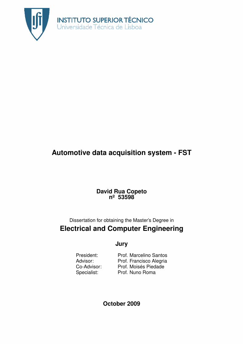
For the measurement when the station is in the Log state, a different method had to be used in orderto be able to characterize the comsumption in the most power intensive phase, that is when a messageshows up in the CAN-bus and it is recorded in the memory and sent through the wireless link. In thisway, the setup shown in figure 2.22 was used. A 0.1±5% Ω resistor was fitted in series with the positivesupply line and the voltage drop between its ends was observed in the difference of 2 channels in anoscilloscope.
Figure 2.22: Setup used for the mobile station’s current consuption measurement.
In figure 2.23 it can be seen there is a voltage drop across the ends of the resistor of 30 mV. Fromthis, the value of the current burst is computed to be 300 mA, a value that is due to the high currentconsumption of the radio transceiver, according to [19, page 8] of 215 mA, while it is in transmit mode.
Figure 2.23: Osciloscope image of a current burst that happens during transmission of a through thewireless link.
26

2.7 Prototype construction
2.7.1 Printed Circuit Board layout
The layout of the mobile station’s printed circuit board was done in Altium Designer, and it’s designhad the size, the easy assembly and the high versatility of the prototype as main concerns. The sizewas reduced by using SMD components as much as possible but still keeping enough space for aneasy assembly, as well as for the wires and connections of the board to it’s exterior connectors. Theversatility and expandability of the board was assured by providing access to some extra wireless radio’spins (RSS signal and 3.3 V regulated supply), to all the microcontroller’s ports, and also by fitting extraplacement holes for “big” capacitors (seen before in section 2.6.1).
In order to reduce noise all the space between traces is filled with ground plane and extra care istaken in the routing around the RTC, following the recomendations of [18], no signal traces are rununderneath the device. The produced board can be found in figure 2.24, and the layout details anddrawings can be found in appendix F.
Figure 2.24: Produced mobile station’s board prototype.
2.7.2 Enclosure
To house the PCB board, a commercial box was modified in order to support the circuit’s connec-tions to the CAN-bus, the USB memory drive, the antenna and the power switch. The CAN-bus cablingrunning across the vehicle uses IP6716 sealed connectors, so a flanged plug is mounted on one of theenclosure’s side panels for superior resistance and isolation as can be seen in figure 2.25. In the samefigure the extra aluminium piece that was fitted to the bottom so that fixation holes could be added can
16Ingress Protection rating. The first number concerns solid materials and the second liquids: 6-Totally protected against dust,7-Protected against the effect of immersion up to 1 m.
27
also be seen. These provide safe holding points when the unit is placed on the vehicle.
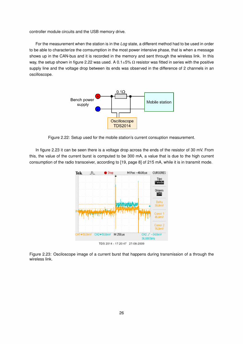
Figure 2.25: Final assembly of the PCB board inside the enclosure fitted with cables to the connectorand power switch. The transceiver adapting cable and the main regulator heatsink can also be seen.
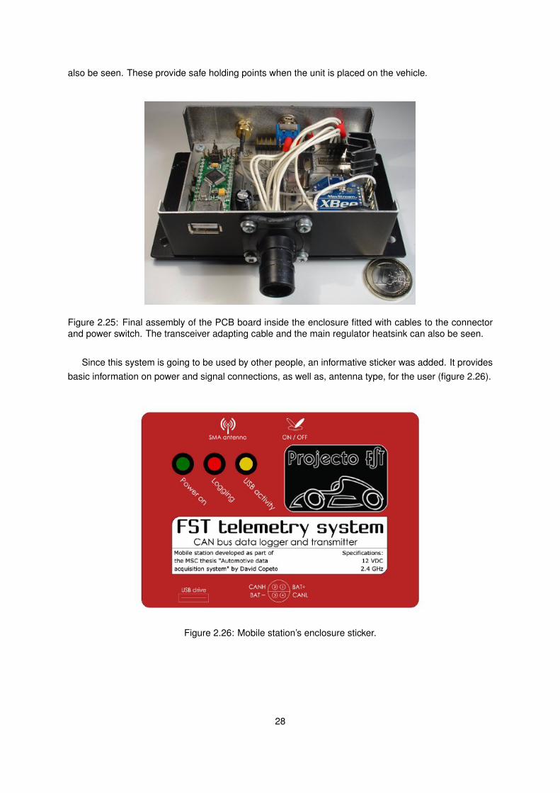
Since this system is going to be used by other people, an informative sticker was added. It providesbasic information on power and signal connections, as well as, antenna type, for the user (figure 2.26).
Figure 2.26: Mobile station’s enclosure sticker.
28

To easily find out the state in which the mobile station is, 3 LEDs were fitted to the top of the box. Intable 2.5, details on the LEDs working conditions can be found. The Logging and USB activity LEDsshould be taken in consideration specially when turning power off in order not to loose any data.
Table 2.5: User information LEDs’ behaviour.
LED Information
Power on When On, station has powerLogging When On, station is in Log stateUSB activity When blinking, warns for USB memory drive usage
The finished mobile station’s prototype can be seen in figure 2.27.
Figure 2.27: Final mobile station’s prototype.
29
2.8 Mobile station Software
2.8.1 Overview
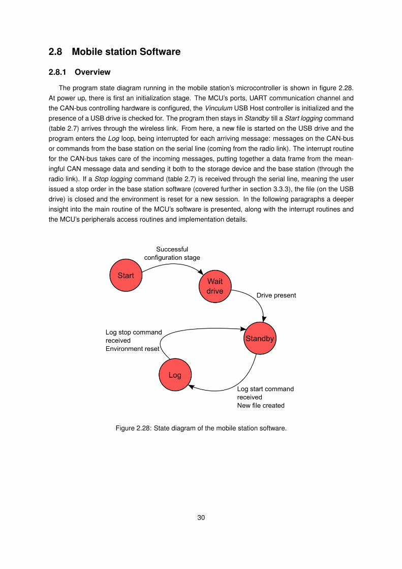
The program state diagram running in the mobile station’s microcontroller is shown in figure 2.28.At power up, there is first an initialization stage. The MCU’s ports, UART communication channel andthe CAN-bus controlling hardware is configured, the Vinculum USB Host controller is initialized and thepresence of a USB drive is checked for. The program then stays in Standby till a Start logging command(table 2.7) arrives through the wireless link. From here, a new file is started on the USB drive and theprogram enters the Log loop, being interrupted for each arriving message: messages on the CAN-busor commands from the base station on the serial line (coming from the radio link). The interrupt routinefor the CAN-bus takes care of the incoming messages, putting together a data frame from the mean-ingful CAN message data and sending it both to the storage device and the base station (through theradio link). If a Stop logging command (table 2.7) is received through the serial line, meaning the userissued a stop order in the base station software (covered further in section 3.3.3), the file (on the USBdrive) is closed and the environment is reset for a new session. In the following paragraphs a deeperinsight into the main routine of the MCU’s software is presented, along with the interrupt routines andthe MCU’s peripherals access routines and implementation details.
Figure 2.28: State diagram of the mobile station software.
30

2.8.2 Main function
The main routine of the microcontroller’s software, starts by configuring the ports and initializing theperipheral devices connected to it (figure 2.2). The CAN-bus controller registers are configured accord-ing to table 2.1 and at this point its interrupt routine (subsection 2.8.6) remains inactive. The USB hostcontroller is also initialized, and the USB drive is detected. If a drive is not present, the MCU holds,querying the Vinculum module until a memory drive is found. Next, the mobile station, receives throughthe serial line the logging session name, chosen by the user at the base station’s software startup wiz-ard (section 3.3.3), which is used to build the names of the files created on the USB memory.
After the configuration stage, the serial interrupt is enabled as the station enters the Standby state.Here, as can be seen in figure 2.28, the software holds until a Start logging command is received fromthe base station (the available commands from the base station are presented further in section 2.8.5).When this happens, a file name is built using the session name truncated to a maximum of 6 characterand a 2 digit number17 (summing up to a maximum of 8 characters for the name - limitation imposed bythe Vinculum). With this name, a text file18 is created on the USB drive (section 2.8.4), then the CANinterrupt is enabled and the Logging state warning LED (section 2.7.2) is turned on. With every changein state and successful completed operation in the mobile station, a feedback message (section 2.8.7)is sent to the base station, so that problems can be spotted by the user.
During the Log state, the arrival of messages on the CAN-bus triggers the CAN interrupt routine(section 2.8.6) or data arriving through the serial line causes, on its turn, the serial interrupt to be called.When a Stop logging commands is received, the Logging LED is turned off and all the interrupts aredisabled, in order to prevent the user from starting a new logging cycle while the mobile station is notyet ready. The file on the USB drive is closed, all the environment is reset and the serial interrupts aremade active again. The system is now ready for a new logging cycle. The flow diagram of the mainfunction can be found in appendix E.2.
2.8.3 Real-Time Clock setup and access routines
The real-time clock value is read whenever a new file is created on the memory drive. There are4 functions related to the RTC: toBCD(), fromBCD(), setTime() and readTime(). The first two, are aux-iliary functions that convert decimal numbers between binary and BCD, and the last ones enable theconfiguration of time registers and current time reads respectively. In order to communicate with theDS3232 the address used on the bus should be 1101000 as found in [18, page 17].
As mencioned already in section 2.2.2, the system has a battery so that continous timekeeping ispossible. In this way, the time on the RTC only needs to be set once (as long as the battery remainsconnected). For this, function rtc_setTime() is used once, being removed from the program in regularoperation19. The flow diagrams of the RTC functions can be found in appendix E.1.
17The file names generated in consecutive logging cycles of the same logging session include a consecutive numbering.18The text (.TXT) file type is the extension chosen for the files stored in the USB drive for their simplicity and universal accep-
tance in various operating systems.19Since the time setting is done in code, after adding the function to the main routine, programming and running the microcon-
troller, it needs to be removed, otherwise it would be executed on every reset of the device.
31

2.8.4 Data storage routines
The communication between the MCU and the USB Host controller through the parallel FIFO issupported on a whole set of functions that had to be written from scratch. These can be separated in 4groups, according to the type of interaction, specified in the following table.
Table 2.6: Vinculum’s functions by interaction type.
Basic Initialization File open File Write
readFIFO() vinculumInit() vinculumOpenFile() vinculumWriteFile()writeFIFO() vinculumDriveStart() vinculumWriteFilePreamble() vinculumWriteBlank()
vinculumDriveStart2() vinculumWriteFileEnd()vinculumWaitDrive() vinculumCloseFile()
The Basic set of functions implements the parallel setting and reading of bits across the 8 data lines(PORTD of the MCU) according to the parallel FIFO protocol timing rules stated in [15, page 7].For the first interactions functions, group Initialization, the functions vinculumInit(), vinculumDriveStart(),vinculumDriveStart2() and vinculumWaitDrive() get the firmware version running on Vinculum, read thedrive’s detection messages and wait for a drive to be inserted, respectively.
Focusing on the interaction set File open, 2 functions are used to perform this action. The first,vinculumOpenFile(), is used to open a file for writing by using the Open File for Write (OPW) commandof the Vinculum firmware[14, page 31]. This function passes the name and date/time information of thenew file to be created. After this command, for each data set to write, the command Write To File (WRF)of the Vinculum firmware[14, page 31] should be used to pass the data (and it’s size) to write on the file.Now, in order to reduce the time it takes to write data to a file, instead of performing a WRF commandeach time there is data to be written, a single WRF instruction is sent right after the file is opened. Thisway, a single WRF is done minimizing the time spent in writes, as there is no need to wait for Vinculumto accept each operation. There is, though, a small drawback to this technique, since with every WRFcommand the size of the data set must be specified. The problem is that at the beginning (when the fileis opened) there is no clue on what is the amount of data that will be written to the file. To overcomethis, the size of the file is always set to the same figure: BYTES_TO_WRITE, a constant defined onthe microcontroller’s program20. The function vinculumWriteFilePreamble() sends the WRF commandto Vinculum with the data size to write as an argument.
In the last group of functions, File write, to interface the USB controller, the vinculumWriteFile() func-tion is called every time a new data set is ready to be stored in the opened file. These data sets canhave any size due to the use of the writing technique mentioned above. There is the need, therefore,to check if there is still enough space for the data set before vinculumWriteFile() is called. That checkis done in the function called by the CAN interrupt, as is further explained in section 2.8.6. If the spaceavailable to complete the size specified at opening time (BYTES_TO_WRITE) is not enough for the dataset “at hands”, space needs to be filled up or else the USB controller will not allow the file to be closed.To do this, function vinculumWriteBlank() fills the remaining space with null data.
20Further ahead in the File write set of functions, will be explained how the problems with setting a constant file size areovercome.
32

If during the log cycle, the file size is reached, a new file must be created in order to continue thedata recording without noticeable interruption. This is accomplished by forcing a new file to be startedwithout the need for the base station control software to intervene. In subsection 2.8.7 the mechanismused to signal this situation to the base station is explained.
When a log session ends, and the file needs to be closed, functions vinculumWriteFileEnd() andvinculumCloseFile(), read the Vinculum’s response to the WRF command and send the Close File(CLF) command respectively.
The flow diagrams for all the Vinculum routines can be found in appendix E.4.
2.8.5 Xbee-PRO/Serial interruption execution
This interrupt routine is triggered whenever data arrives (from the base station) on the serial lineconnected to the radio transceiver. The serial line is configured to work at a rate of 115200 baud with8 bits, 1 stop bit and no-parity. As can be seen in table 2.7, only 2 different actions can be triggeredwith this interrupt routine. If the character ’g’ is received, the mobile station changes its state to Log anda message is put on the CAN-bus for all the nodes in the network to reset their timers, if instead a ’s’arrives, the Log state is interrupted. In appendix E.14 the flow diagram of the serial interrupt function,isrSerial(), is deppicted.
Table 2.7: Actions triggered by the serial line interrupt routine.
ASCII character received (hex value) Command name Action
g (0x67) Start logging Change state to Logs (0x73) Stop logging Change state to Standby
2.8.6 CAN-bus interruption execution
The filters on the MCU’s CAN controller are set so that messages comming from nodes with anyCAN_ID are accepted, as well as any kind of message type. In this way, everytime a new CAN mes-sage is put on the bus, isrCanrx1() is called. In order to prevent reentrancy, first the CAN-bus interruptsare disabled while this interrupt routine is being executed. Then the message is fetched from the CANcontroller buffers and, if there is still space in the file (BYTES_TO_WRITE hasn’t been reached) datais recorded on the USB drive by calling vinculumWriteToFile() (seen above in section 2.8.4) and alsosent to the base station through the wireless link by calling sendFrame() (covered further ahead insection 2.8.7). If the file has no more space, a “forced” log stop condition happens, to which followssignaling to the base station and an immediate closing of the file and opening of a new one (in the sameway it has been described above in section 2.8.2) so that logging can continue. The flow diagram forthe CAN interrupt routine can be found in appendix E.15.
33
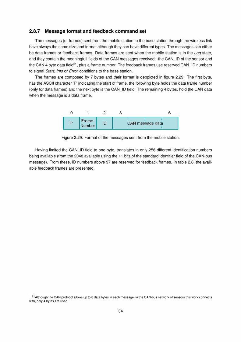
2.8.7 Message format and feedback command set
The messages (or frames) sent from the mobile station to the base station through the wireless linkhave always the same size and format although they can have different types. The messages can eitherbe data frames or feedback frames. Data frames are sent when the mobile station is in the Log state,and they contain the meaningfull fields of the CAN messages received - the CAN_ID of the sensor andthe CAN 4 byte data field21, plus a frame number. The feedback frames use reserved CAN_ID numbersto signal Start, Info or Error conditions to the base station.
The frames are composed by 7 bytes and their format is deppicted in figure 2.29. The first byte,has the ASCII character ’F’ indicating the start of frame, the following byte holds the data frame number(only for data frames) and the next byte is the CAN_ID field. The remaining 4 bytes, hold the CAN datawhen the message is a data frame.
Figure 2.29: Format of the messages sent from the mobile station.
Having limited the CAN_ID field to one byte, translates in only 256 different identification numbersbeing available (from the 2048 available using the 11 bits of the standard identifier field of the CAN-busmessage). From these, ID numbers above 97 are reserved for feedback frames. In table 2.8, the avail-able feedback frames are presented.
21Although the CAN protocol allows up to 8 data bytes in each message, in the CAN-bus network of sensors this work connectswith, only 4 bytes are used.
34

Table 2.8: Set of feedback frames used by the mobile station.
ID number Type Description
98 Info Normal Log stop99 Info Forced Log stop
100 Start Start of program101 Start Configuration of CAN communication102 Start Date/Time set103 Start Vinculum start-up104 Start Start of standby cycle105 Start Start of new log file106 Start Start of log cycle107 Start Drive start108 Info Extra data109 Info Drive present110 Info Drive not present111 Info File created/opened112 Info Ending file113 Info File closed114 Info Log start acknowledge115 Info Sensor info116 Error Vinculum can not change to SCS117 Error File can not be created/opened118 Error File could not be closed119 Error Other error120 Error CAN error121 Info CAN time reset
The feedback frames are used to provide feedback to the base station on which state the mobilestation software is in, as well as, give information on the result of the interaction with the peripheral de-vices and warn on possible error conditions. The function sendFrame() is the routine used for sendingframes through the serial line and its flow diagram can be found in appendix E.16.
35

36

Chapter 3
Base Station
3.1 Overview
The base station is the part of the system that is located off-track (figure 3.1). Its hardware is formedby a wireless transceiver and a PC. The wireless transceiver in the base station completes the RF linkbetween the two parts of the system as seen already in figure 1.3. The PC runs the user interface soft-ware to the system, allowing both “online” data collection and “offline” data analysis. The connection ofthe radio module to the computer is done with the help of the same XBee development board used fordevice characterization (figure 2.9).
Figure 3.1: Base station.
37

3.2 Programming language choice
The first choice when developing the system’s user interface, was the programming language. Thisis an important step as the chosen software tools can condition the development speed and freedomas well as the application’s final overall performance. In this way, the chosen “software package” must,above all, include libraries to access the serial port (as the interface with the radio module is done inthis way), have graphic libraries that allow the creation of a fairly complex graphical interface and alsoallow the development in an open-source OS1.
The options taken in consideration were the use of JAVA, Matlab, Labview and C. The first two,although managing almost all the requisites and already including complete graphic libraries were setaside beacause the applications tend to become “heavier” (speedwise). Labview, was thought as notbeing appropriate to the kind of application and C, although producing the “lighter” applications lacksobject-oriented programming. In this way the chosen base language was C++. Being a high level lan-guage with low-level functionalities, allows a good performance, and is a good tool to implement theversatility desired for the application.
As to the graphical interface, it is developed using the Qt Framework together with the Qwt libraries.Qt is multiplatform graphical package, which means that software migration between different operatingsystems is easier, and it includes a large collection of graphical widgets2 to incorporate in applications.Lastly, the Qwt libraries are used to add a few visualization widgets that make showing data to the usermore efficient and enjoyable.
1The experience of the author with certain languages is also a very important point, although, in the case of this work, notdecisive.
2A graphical widget is the general name of any item that composes a graphical interface, like buttons, windows or icons.
38

3.3 Software
3.3.1 Objective
The general purpose of the software running on the base station is to give the user an interface tothe system. With more detail, the graphical interface should be an easy and attractive tool able to plotincoming data, have a versatile and reconfigurable structure so that it allows different sized CAN-busnetworks to be monitored, accept different sensors and sample rates, be a tool to perform analysis onpreviously gathered data and also be able to recover data stored on the mobile station’s USB memorydevice.
3.3.2 Structure
The application is structured according to figure 3.2. Since it is possible to configure the softwarefor the kind of session and network it will work with, an important piece is the startup wizard. This pre-application configuration tool guides the user into the sort of session he wants, asking for all the infor-mation needed to build the environment. This results in the main application window and the databasebeing built. Deppending on the type of session the database is filled up with data values, in the case ofan Offline session, or is empty, in the case of an Online session. Likewise, the data source and structureof the main window also depends on the type of session. The data is completly loaded at startup if itssource is the hard drive or the USB memory drive, or, in the case of an Online session it is received bythe serial interface “block” comming from the Zigbee radio. After the main window is built, the user hasthe possibility to change a few details in the visualization of the items and also control the state of themobile station.
3.3.3 Functionality details
In the following paragraphs the functions and characteristics of the core pieces of the software arepresented. In appendix G.1 the class diagram of the base station software is deppicted.
Wizard
The wizard is composed of a series of input fields designed to help start the application (figure 3.3),and cannot be skiped. The user must complete the forms in order to properly build the application for thedesired purpose, although in an Online session some of the information entered can be later modified.
When the option for a Create... (Online session) is made, in a first page the name of the session isentered and the option to read a CAN-bus network composition from a previously created session fileis presented (figure 3.4). Then in a second page the CAN-bus network arrangement is requested. Inorder to properly build the main window, the user provides a name, the CAN-bus ID and type of eachsensor, and also choses if the sensor data is to be viewed in the plot area, as deppicted in figure 3.5).
39

Figure 3.2: General structure of the base station software.
For the case of a Load... (Offline session), the user simply points to the session file (the file typesare refered further in the Database paragraph) and the main window is built without further informationinput (figure 3.6).
If the third option is selected, the Retrieve... (Offline session), the user points the USB memory’s fileto be read and then adds the information regarding the type of each sensor found in the file, which isnecessary for a correct loading and plotting of the values (figure 3.7).
40

Figure 3.3: Wizard start page.
The application’s wizard is accomplished using a series of classes, one for each page in it. Worth ofreference is the method accept() of class startWizard which is called when the user presses the Finishbutton. Here, for every type of session, the database is built and for the Offline type of sessions, datavalues are read from files and the database is built.
Database
The structure holding the data is organized as a list of sensors. For each sensor, besides the datavalues, details on name, CAN-bus ID and type are kept, and whether the values should be ploted or not(Online session). There are 8 types of sensor available: Tire temperature, Throttle position, Steeringposition, Wheel speed, Suspension displacement, Engine coolant temperature, Engine RPM and SineWave (for testing purposes). For each type a different display widget exists as seen further ahead.
This database is always built based on the inputs of the user to the wizard and can be changed whilethe program is running, in the case of an Online session, and is “filled up” with the incoming data fromthe serial interface. For the Offline sessions, it is completly loaded with data values at startup.
In order to save the data on the PC’s hard drive, two types of file are used. One, the .sfl file, registersall the parameters concerning a logging session, namely date and time, number of sensors, numberof values per sensor and number of runs (explained further in the Online Window paragraph), amongothers. The second type is a .txt file per each sensor logged, that stores all the data values received aswell as the sensor details. Example contents of these files can be viewed in appendix G.2.
Two classes are used for organizing data, the sensor and the dataBase classes. The first has justone method, to create objects that populate the list existing on the second. Notice that for each sensorobject created, a new output file (to store the data values) is created too.
41
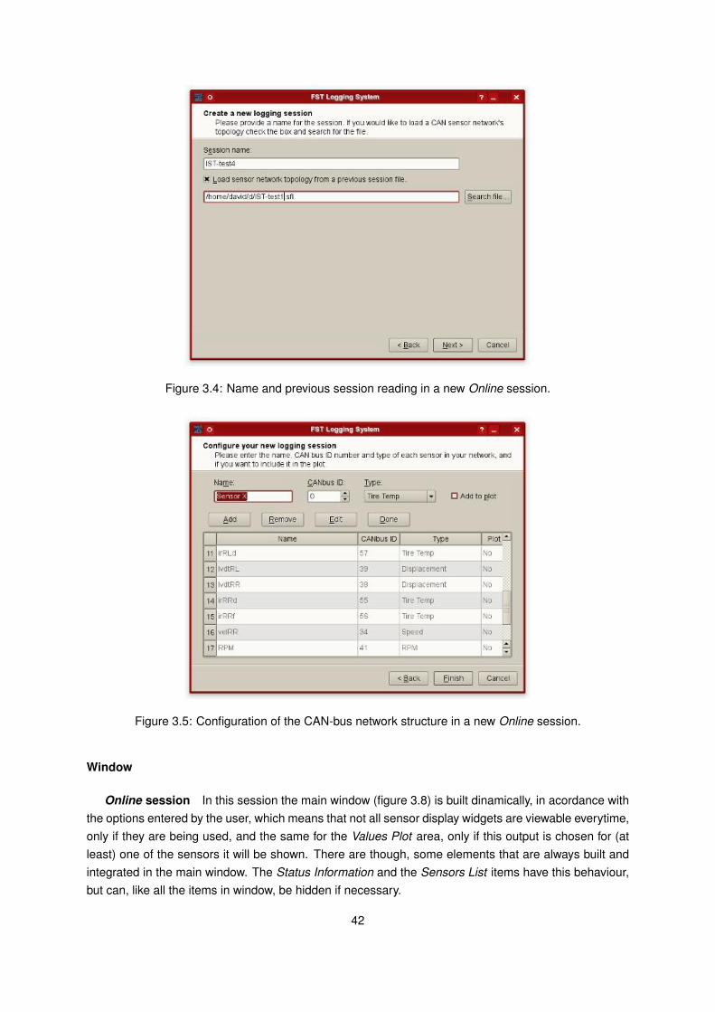
Figure 3.4: Name and previous session reading in a new Online session.
Figure 3.5: Configuration of the CAN-bus network structure in a new Online session.
Window
Online session In this session the main window (figure 3.8) is built dinamically, in acordance withthe options entered by the user, which means that not all sensor display widgets are viewable everytime,only if they are being used, and the same for the Values Plot area, only if this output is chosen for (atleast) one of the sensors it will be shown. There are though, some elements that are always built andintegrated in the main window. The Status Information and the Sensors List items have this behaviour,but can, like all the items in window, be hidden if necessary.
42

Figure 3.6: Finding a previous session file (Offline session).
Figure 3.7: Adding the type information when data is read from the USB memory’s file (Offline session).
There is a sensor display widget for each type of sensor in the system for displaying its current value.These are built using classes dialMeter, scaleMeter and steeringMeter. In figure 3.9 the 8 different dis-plays available are shown.
43

Figure 3.8: Main window in an Online session.
Figure 3.9: The 8 sensor display widgets. (a) Engine RPM, (b) Wheel speed, (c) Suspension displace-ment, (d) Tire temperature, (e) Steering position, (f) Sine Wave, (g) Engine coolant temperature, (h)Throttle position.
The Values Plot item, displays the incoming data for the selected sensors and enables zooming andaxis dragging using the mouse buttons, besides showing coordinate value with just a click. The currentplot image can be saved as an image file (.jpg, .png or .bmp) by chosing this option on the File menu.
44

The Status Information item, that can be seen in figure 3.10a, besides holding the log state controlbutton, from which the user can issue the commands seen in table 2.7, shows the name of the file beingwriten in the USB memory drive, the current wireless link data rate in kB/s and the current state at whichthe mobile station is. It also includes an activity log so that the user has feedback of what is “going on”in the embarked subsystem.
Everytime the log “Start” button is pressed a new run begins. Consequently a new file for eachsensor to hold the data from the run is created and the Values Plot is reset.
If there is a change in the topology of the CAN-bus network during a session, the user can, throughthe Sensors List item (figure 3.10b), make the suitable changes, being able to add or delete sensordisplaying widgets (and consecuently adding or deleting them from the database).
(a) Status Information item (b) Sensors List item
Figure 3.10: The two constant components of the Online session main window.
Offline session For both modes of this session type (load from hard drive or load from USB drive)the main window has a static structure. There are only two elements, the Sensors List and the PlotArea, which make available all the controls over each trace on the plot and show the enabled tracesrespectively.
The Sensors List, presents all the sensors available for data analysis. By selecting one, its optionsbecome available: it can be hiden and its color and markers can be changed. Because in the same plotarea, different quantities are to be represented using only one ordinate axis, every sensor data set (orcurve) can be multiplied or have a constant summed to it.
The large Plot Area item uses the same widget as the above mentioned Plot Area, it enables theuser to have a good resolution when analyzing the data. The current plot image can also be saved asan image file in the same way as described above.
In order to build the window and its items two classes are used, windowItem and mainWindow. Thefirst, is the class of the sensor visualization items and holds their details, the second has the methodsto build every kind of item including the Status information, Sensors List, and Values Plot /Plot Area.
45

Figure 3.11: Main window in an Offline session.
Serial interface
Is the piece responsible for getting the data from the serial port to the right place in the databaseby interpreting the messages that arrive. The CAN_ID field (section 2.8.7) of the frames sent throughwireless is used to evaluate each frame and from there the values are stored in the correct databaseentry and a signal is sent for the sensor visualization items on the main window to update their values.
The serial interface is implemented through the serialComms class. For a better performance themain serial interface method, run(), is implemented inside a thread.
46

Chapter 4
System performance
In order to evaluate the entire system’s performance, tests are run in two different environments -the bench and the track. The differences in the two locations for testing are mainly resumed to theconditions of wireless data propagation, size of the CAN-bus network which it connects to and also theconditions in terms of mechanical stress and electrical noise.
4.1 Bench tests
In the bench, under a fully controlled surrounding the system’s working condition is thougth as beingideal. Besides being the system’s development environment is also where optimal conditions in termsof power supply, wireless distance and mechanical stress are met.
4.1.1 CAN-bus network emulation platform
Since this work has the objective of connecting with a network of nodes supported on a CAN-bus,during its course, a platform for tests was developed so that the interaction with such network couldbe emulated. This testing platform is composed of simple modules that can be connected through aCAN-bus and generate data in a similar way as the CAN-bus network nodes of the vehicle do.
Each module consists of a CAN-bus communication capable microcontroller (PIC18F4585) fittedwith minimal connections and components and a CAN-bus transceiver (MCP2551) as can be seen inthe block diagram of figure 4.1.
47

Figure 4.1: Block diagram of the CAN-bus network emulation platform.
The built platform, deppicted in figure 4.2, is formed by 4 of these modules that can be freely con-nected/disconnected to the CAN-bus. Each node of the testing network is programmed to output (byputting a CAN-bus message on the bus) a sine wave1 with a certain frequency. By using a sine wave,the data generated in each node is known a priori and so it can be easily spoted if the logging of theCAN-bus messages is being successful.
Figure 4.2: CAN-bus network emulation platform built.
1Constructed out of a sample of 91 values per quarter of period
48

4.1.2 CAN-bus interruption routine timming
As explained in section 2.8.6, each time a new message is put on the CAN-bus, the mobiles station’sCAN interruption routine picks it up and sends the CAN-bus messsage data field through the wirelesslink (using the UART to connect to the radio transceiver). Since the MCU can only deal with one CAN-bus message at a time, the amount of time this process takes is crucial to understand what is theleast time spacing that messages put in the CAN-bus can have between them. In order to quantifythe time a function takes, a random MCU i/o pin is set high throughout its duration and captured withan oscilloscope. For this test, one node of the CAN-bus network emulation board is connected to theCAN-bus, and it sends messages periocally as explained above.
The two important actions made by this routine are the recording of the data frame on the USBmemory drive (call to function vinculumWriteToFile()) and sending it through the serial link to the radiomodule (call to function sendFrame()). Likewise the time taken by each of these function calls is mea-sured and the results can be seen in figure 4.3.
(a) isrCanrx1() in blue and vinculumWriteToFile() in green (b) isrCanrx1() in blue and sendFrame() in green
Figure 4.3: Results of the measurements of vinculumWriteToFile() and sendFrame() function calls’ time.
From figure 4.3, it is easy to understand that the reason for the overall time, taken by the CANinterruption routine, is the call to function sendFrame(), which takes 448 µs, and not the call to vincu-lumWriteToFile() that takes 8 µs. This result is in discordance with the aproximated transmission timecomputation that can be done based on the baud rate setting of the UART communication channel.As mencioned before (section 2.8.5), the baud rate is set to 115200 baud, which means that the lineswitches state 115200 times per second. Since each switch in state is equivalent to 1 bit, the time a bittakes to be transmitted is:
tbit =1
115200= 8.681µs, (4.1)
and for a data frame with 7 bytes (section 2.8.7) it makes the time to transmit a message:
tmessage = 7 × 8 bit × tbit = 486.1µs, (4.2)
49

which is higher than the measurement made. The difference is found to be due to the MCU baudrate setting. According to [11, page 232], for a device’s oscillator frequency of 40 MHz and a UARTbaud rate setting of 115200 baud, the actual rate has a positive error to the set value and is 125000baud. If the time per bit and the time per message are computed again:
tbitREAL =1
125000= 8µs→ tmessageREAL = 7 × 8 bit × tbitREAL = 448µs, (4.3)
which agrees with the measurement of figure 4.3b.
4.1.3 Wireless link maximum throughput
In order to obtain the efective maximum data transmission rate achieved by the wireless link betweenthe mobile and base stations, the test setup of figure 4.4 is used, where d = 1 m.
Figure 4.4: Setup for the maximum throughput measurement on the bench.
Since this test has the objective of studying the behaviour of the wireless connection between sta-tions, the mobile station is disconnected from the testing CAN-bus and the main program is changed sothat data frames containing the sine wave (used in the same way as explained before) values are sentto the base station at a certain frequency. This way, by changing the frequency at which the frames aresent and computing the amount of bytes arriving per second2 at the receiving end (base station), thethroughput of the wireless link can be obtained as can be seen in figure 4.5.
2The throughput value is computed by making an average of the bytes/s arriving in a period of 60 seconds.
50

Figure 4.5: Results of the measurements of the wireless link throughput in the bench. Expected valuein red and the system’s value in blue.
A maximum throughput of 9.61 kB/s is achieved by the wireless link with a relative error to the ex-pected of 0.04.
4.2 Track tests
The system was also tested in a real environment, that is, connected to the vehicle’s CAN-busnetwork of sensors, with the vehicle running on the practice track mencioned before (figure 2.6). Theobjective was to evaluate the performance of the system in the ambience in which it was designed towork and also to understand if its enrollment in an electrically noisy system would cause failure. Besidesthe functioning considerations, overall mechanical design and resistance was also evaluated.
The CAN-bus network of sensors was composed of 3 nodes3 placed throughout the vehicle as canbe seen in figure 4.6.
3Further details on the CAN network nodes and sensor specifications are considered out of the scope of this work.
51

Figure 4.6: Sensors network on the vehicle. The nodes (green) are connected to the mobile station (red)through the CAN-bus (yellow). Sensors: tire temperature (orange), wheel speed (blue), suspensiondisplacement (dark red), throttle (yellow), engine RPM (red), engine coolant temperature (pink) andsteering angle (gray).
4.2.1 Performance for different base station positioning
With the vehicle running on the track, the distance between the mobile and the base station is thekey factor, for the good operation of the system, being changed with time. In this way, it is of interestto study what is the best location around the course to place the mobile station. Two different locationsare used and they are chosen for both being out of the limits of the track and being believed to turnout the best results in terms of wireless propagation, due to having less obstacles or less distance tothe track. In figure 4.7, the two locations can be seen. Location 1 (blue square) is on top of a smallgarages building, approximately 4 meters high, from where all the track can be seen, and Location 2(red square) is by the course’s start line, at approximately 1.5 meters in height.
52

Figure 4.7: Practice track image with points of interest. Location 1 (blue square), Location 2 (redsquare), Track point 1 (green circle), Track point 2 (yellow circle), Trees (green elipse) and Low area(orange elipse).
In order to evaluate the wireless link, the emulation platform (explained above in section 4.1.1) isadded to the CAN-bus network already in the vehicle, with just one node generating a sine wave, inorder to, as before, have “known” data being generated on the embarked system. By looking for im-perfections on the sine wave shape (figure 4.8, captured with the Save plot image function describedin section 3.3.3), it was possible to identify the spots on the track where the wireless connection be-tween the mobile and the base station was temporarily broken as the vehicle performs several laps.The “higher” connection loss spots of the track are marked on figure 4.7. In this figure, it can be seenthat with the base station at Location 1 the critical Track points are 1 and 3, which is belived to be dueto trees in the station’s line-of-sight propagation4, and for Location 2 the critical Track point is number 2,due to the track going through a lower ground area at that point.
Overall, the performance in both locations is similar, as the position of objects in the middle of thetrack area creates dificulties for both in different spots, and the fact that from one Location to the other,the distance to the vehicle is exchanged by height (which translates in line-of-sight propagation betweenstations).
Although the method used enabled some weaker connection spots on the practice track to be iden-
4Line-of-sight propagation refers to the travelling of radio signals in a straight line with no obstructions.
53

Figure 4.8: Example of a sine wave with short imperfections (black circle).
tified, the peformance/coverage of the connection is good, as, considering the average speed at whichthe vehicle performs the laps (measured to be always above 40 km/h on this track), the losses in “live”sensor data are acceptable and barely noticed, also due to the frequencies at which data is acquiredfrom each sensor (in the case of the test realized: 10 Hz for all sensors except temperature - 1 Hz). Infigure 4.9 a saved image of the plot area shows an example of the data gathered by the system at thepractice track.
Figure 4.9: Data acquired at the practice track. Temperatures of the tire’s inside (pink) and outside (red),the throttle’s position (blue) and the engine’s RPM (green).
54

4.2.2 Wireless link maximum throughput
The efective maximum data transmission rate on the track was obtained for what is thought as oneof the worst case scenarios, when the car is passing by Track point 1 (figure 4.7) and the base stationis at Location 3, which differs from Location 2 on the height, being this approximately 80 cm off theground. The testing scheme is in all similar to the one of figure 4.4 for the bench test, with the differencebeing the distance that separates the two stations d ' 300 m, as can be seen in figure 4.7. The result ofthe throughput capability of the wireless link can be seen in figure 4.10.
Figure 4.10: Results of the measurements of the wireless link throughput in the track. Expected valuein blue and the system’s value in green.
The maximum throughput achieved by the system in this case was 4.45 kB/s with a relative error of0.36 to the expected, and 4.28 kB/s with a 0.08 relative error to the expected. The first value is obtainedwith a high relative error, meaning a great amount of losses, and so the second value is considered asthe maximum with the system in acceptable working conditions.
55

4.2.3 Considerations on mechanical behaviour
The mobile station enclosure proved to be resistent to the vibrations of the vehicle, and the USBmemory drive socket is strong enough to hold the drive without this one falling. The station’s bottom fix-ation piece was also able to safely hold the unit in place just using zip ties as can be seen in figure 4.11.
Figure 4.11: Mobile station installation on the vehicle using zip ties for secure hold.
56
Chapter 5
Conclusions
In this project, the development, construction and deployment of a CAN-bus data logging andtelemetry capable system was proposed. To reach this objective both COTS parts and original cir-cuit design were put together with software developed for two different platforms and the result wastested in a real world cenario. The work was divided in two parts: an embarked sub-system (the mobilestation in chapter 2), composed of a microcontroller, a CAN-bus interface and a storage unit and aninterface sub-system (the base station in chapter 3), composed of a PC running an application with agraphical user interface (GUI). In order to connect the two sub-systems, a wireless link was studied(section 2.4.2) and used (section 2.4).
Both stations are original contributions of this thesis and the mobile station hardware was developedhaving in mind the balance between cost, performance and ease of integration, particularly the use ofthe Vinculum USB host controller (section 2.5.2) together with a USB memory drive, proved a goodoption when compared to more classic approaches like, SD or MMC cards and EEPROMs. In themobile station’s embedded software, the time taken by the critical routines (section 4.1.2) was minimizedin order to collect all the messages put in the CAN-bus and, to the extent tested, CAN-bus messageswere not lost.
Regarding the base station, its hardware was kept simple in opposition to its software, which grew incomplexity because of the project objective of having a dynamic and versatile user interface. The GUIwas developed in a Linux OS but using libraries that allow an easy port to other operating systems.
Of note is the fact that this work was developed to interface with other systems being developed atthe same time - the CAN-bus network of sensors (section 4.2). This situation, which is not easily foundin the academic course, proved very challenging.
The objective, presented in section 1.1, was completly fulfilled by the delivery of a working systemwith reliable CAN-bus message recording and wireless transmission of data up to 4.28 kB/s (valuethat corresponds to the situation tested at the practice track used). This throughput proved enough totransmit the data generated by an existing CAN-bus network of 20 sensors with the vehicle runningseveral regular practice laps and reaching an aproximate 300 m maximum distance between both endsof the wireless link.
The wireless link has, none the less, dificulty to comply with obstacles in the transmission path,being line-of-sight propagation the ideal for the XBee-PRO radios, which means a track completely freeof obstacles. Due to this, and the fact that no flow control or acknowledge schemes are used in the
57

wireless transmission of data in either direction, live data from the mobile station can be lost as seen insection 4.2.1.
Concerning the data recorded on the USB memory drive, its safety is only compromised if properclosing of files does not takes place, which can (as proved by experience on test runs) happen, whenthe vehicle, for example, undergows a problem and its power needs to be swiftly cut. The solution wouldpass by modifying the recording method to make it more robust in the presence of sudden power failures.
5.1 Future work
As future enhancements of this system, it is proposed the further exploitation of the degree of free-dom presented by the antenna type. By using a more directional antenna on the base station, propa-gation problems could be mitigated. Also the use of flow control and the implementation of a minimalhandshaking protocol would contribute to less losses on the transmission. Another option would be tomove to WiFi technology which would provide a larger bandwidth and also make easier the implemen-tation of a transport layer protocol like TCP. In order to reduce the power consumption of the mobilestation a sleep state can be implemented and the telemetry scheme could be changed in order to runin tracks with a lot of obstacles by using the information on the radio signal strength to choose when themobile station should transmit.
On the base station’s software, it is proposed an enhancement of the serial routine, so that it be-comes less CPU “intense”, the inclusion of a “driver comparison mode” and also the possibility to dofurther configurations of the mobile station.
5.2 Cost analysis
As mentioned before, the cost of components was one of the parameters taken into account through-out this work, and with special importance in the choice of the COTS devices included in the system.The amount and cost of each component can be found in table 5.1, together with the efectively paidvalue and supplier’s name.
The difference between the unit price (multiplied by the amount) and the efectively spent for eachcomponent has to do with added shipping costs, orders with miminum quantities, mistakes in compo-nent order, manufacturers samples service, or free components from miscellanious sources. Left offthe table, due to the difficulty in computing a cost, are screws, heat shrink tube, solder and wires. Alsoleft out, is the PC, needed to run the base station software but left out as any computer with a USB portcan be used.
In order to compute the total cost of the system, 3 different cases are appreciated and the result canbe seen in table 5.2. In the cost of the first (and only) prototype built, which has the highest cost, all themoney spent is considered. For the case of building a second prototype, the cost drops dramaticaly asall the material that had to be bought in large quantities for the first prototype is available at unit price,and particularly in the case of the Development Kit Xbee-PRO, one of these is enough for 2 systems tobe built. Lastly, the production case, takes in consideration a large number production (considers unit
58

Table 5.1: Prototype cost’s breakdown.
Component Amount Unit price (e) Spent (e) Supplier
Aluminium Box RETEX 105x35x75 mm 1 6.9 6.9 DimofelVoltage Regulator LM7805 TO-220 1 0.2 0.2 RadipeçasCrystal 10 Mhz 1 0.16 0.16 RadipeçasOn/Off Toggle Switch 1 1.16 1.16 Radipeças5 mm LED Plastic Support 3 0.1 0.3 Radipeças5 mm Red LED 1 0.07 0.07 Radipeças5 mm Green, Yellow LED 2 0.08 0.16 RadipeçasLithium Coin Cell 3 V 200 mA 1 3.56 3.56 RadipeçasMCU PIC18F4685-I/PT TQFP 1 9.58 0 FarnellRTC DS3232SN SOIC 1 10.42 0 FarnellVoltage Regulator TC1264-3.3 SOT-223 1 0.8 0 DigikeyVinculum module VDIP1 1 24.85 56.66 FTDI onlineRadio Transceiver Xbee-PRO U.FL 1 27.91 27.91 FarnellDevelopment Kit Xbee-PRO 1 179.8 179.8 FarnellCAN transceiver MCP2551 1 1 0 FarnellCable u.fl-SMA 75 mm 1 7.9 17.5 RSConnector 4vias Sureseal w/flange (min 5) 1 3.02 15.1 RSPins Sureseal male (min 10) 2 0.31 6.2 RSPins Sureseal female (min 10) 2 0.58 11.6 RSEnclosure Sticker color print 1 2.6 5 Let’s CopySpray paint mate black 1 3 3 Leroy MerlinPCB fabrication 2layers 1 25.86 63.25 Beta LayoutAntenna 2.4 GHz SMA 1 11.48 11.48 RSHeatsink TO-220 1 0.5 0 RSStick-on feet (bag of 108) 4 9.25 0 RSPCB Socket 20ways vertical (min 5) 1 2.14 10.7 RSSMD resistors and capacitors 22 0.86 17.6 Farnell
price for every component and no samples), which reduces the cost. To have a complete figure of theproduction case total it should also be added the assembly and testing cost.
For the first prototype and the production cost cases, a great cut could be achieved by not using theDevelopment Kit Xbee-PRO, because this is only used to provide the interface boards between the PCand the radio module on the base station. Simpler and cheaper interfaces are available on the market(for example Sparkfun’s XBee Explorer USB for e17.48) or a custom board could be developed. Thecost for all three cases in this scenario can also be seen in table 5.2, which are computed by deducingthe Development Kit Xbee-PRO cost, adding 2 of the mentioned interface boards and 1 more RadioTransceiver Xbee-PRO U.FL.
Table 5.2: Total cost of the system for 3 different cases.
Total cost Value (e) Value by cutting the Development kit (e)
First prototype 400.41 283.48Second prototype 85.2 148.07Production 298.69 271.66
59

60

Bibliography
[1] Telemotive AG. https://www.telemotive.de/4/en/. accessed 2-Dez-2009.
[2] Cosworth. http://www.cosworth.com. accessed 1-Dez-2009.
[3] Robert Bosch GmbH. CAN Specification Version 2.0, 1991.
[4] IEEE. Standard 802.11g™-2003 - LAN/MAN Wireless LANS. Technical report, IEEE, 2003.
[5] IEEE. Standard 802.16™-2004 - Broadband Wireless Metropolitan Area Network. Technical re-port, IEEE, 2004.
[6] IEEE. Standard 802.15.1™-2005 - Wireless Personal Area Networks. Technical report, IEEE,2005.
[7] IEEE. Standard 802.15.4™-2006 - Wireless Personal Area Networks. Technical report, IEEE,2006.
[8] Fairchild Semiconductor International Inc. LM78XX/LM78XXA 3-Terminal 1A Positive Voltage Reg-ulator, 2008.
[9] Microchip Technology Inc. Application Note 713 - Controller Area Network (CAN) Basics, 2002.
[10] Microchip Technology Inc. High-Speed CAN Transceiver MCP2551, 2003.
[11] Microchip Technology Inc. PIC18F2682/2685/4682/4685 Data Sheet, 2007.
[12] KVASER-The CAN Protocol Tour. http://www.kvaser.com/can/intro/index.htm. accessed 9-May-2009.
[13] Lawicel-CANUSB. http://www.canusb.com. accessed 2-Dez-2009.
[14] Future Technology Devices International Ltd. Vinculum Firmware User Manual Version 2.05, 2004.
[15] Future Technology Devices International Ltd. VDIP1 Vinculum VNC1L Prototyping ModuleDatasheet Version 0.92, 2007.
[16] Future Technology Devices International Ltd. Vinculum VNC1L Embedded USB Host Controller ICDatasheet Version 2.0, 2008.
[17] Stack Ltd. http://www.stackltd.com. accessed 2-Dez-2009.
[18] Inc. Maxim Integrated Products. DS3232 Extremely Accurate I²C RTC with Integrated Crystal andSRAM, 2007.
61

[19] MaxStream. XBee™/XBee-PRO™ OEM RF Modules Data Sheet, 2006.
[20] Bhavneet Sidhu, Hardeep Singh, and Amit Chhabra. Emerging Wireless Standards - WiFi, ZigBeeand WiMAX. World Academy of Science, Engineering and Technology, 21, January 2007.
[21] Race Technology. http://www.race-technology.com. accessed 2-Dez-2009.
62

Appendix A
Formula Student and Projecto FST
In this appendix, a short introduction to the Formula Student competions can be found, as well assome insight on the team Projeto FST and the vehicle FST03.
A.1 Formula Student
Adapted from What is Formula Student? at formulastudent.com:
Started in the United States by SAE in 1981, the Formula SAE programme was consid-ered to be very worthwhile in providing students with excellent learning opportunities andpractical skills. In europe the IMechE accepted the management of the European venturein a partnership with SAE. Formula Student (the name given to the event held in England)is different from Formula SAE in that it is designed to be a progressive learning exercisethroughout the different classes. However, the same rules are used for both Formula Stu-dent and Formula SAE (with some minor changes).
Formula student provides the students with a real-life exercise in design and manufactureand the business elements of automotive engineering. It teaches them all about team work-ing, under pressure and to tight timescales. It demands total commitment, lots of late nights,and many frustrations and challenges along the way, but the result is the development ofhighly talented young engineers.
For the purpose of the competition, the students are to assume that a manufacturing firmhas engaged them to produce a prototype car for evaluation. The intended sales market isthe non professional weekend autocross or sprint racer. Therefore, the car must have veryhigh performance in terms of its acceleration, braking, and handling qualities. The car mustbe low in cost, easy to maintain, and reliable. In addition, the car’s marketability is enhancedby other factors such as aesthetics, comfort and use of common parts. The challenge tothe team is to design and fabricate a prototype car that best meets these objectives. Eachdesign is compared and judged with other competing designs to determine the best overallcar.
The teams have their work judged by Industry specialists and demonstrate the perfor-mance of the car. It is not simply the fastest car that wins, students have to balance speed
63

with safety, reliability, cost and good handling qualities.
A.2 Projecto FST
The team from IST is formed by students of both mechanical and electronics engineering. It hasalready successfully delivered 3 prototype vehicles, from which 2 are still in the active. This work isaimed at the latest built prototype, the FST03, who’s main technical specifications can be found intable A.1.
At the moment the team is in its fourth formation whom is working on the next prototype vehicle - theFST04.
Table A.1: Technical specifications of FST03.
General dimensions
Overall Length 2827 mmOverall Width 1450 mmOverall Height 1214 mmWheelbase 1650 mmTrack 1200 mm(front) 1150 mm(back)Weight with 68 kg driver 131.85 kg(front) 161.15 kg(back)
Frame
Construction Steel tube space frameMaterial 4130 alloy steel tube
Engine
Model 2001 Honda CBR 600 F4iCylinders 4Displacement 599 ccPower 80 hp at 11500 RPM (measured at the wheel)Exhaust header design 4-2-1 equal length
Suspension
Type Double unequal length A-Arm. Pull rod actuatedvertically oriented spring and damper.
Transmission
Type Torsen Differential FSAE Special
Wheels
Rims 13'' Carbon Fiber with an 7050 Aluminium CenterTire AVON 13'' Slicks
Body
Material Fiberglass
64

Appendix B
CAN-bus protocol
In this appendix an introductory explanation of the CAN-bus protocol can be found and also themethod to compute the CAN-bus controlling hardware register’s configuration values.
B.1 Message arbitration
In order to support a non-destructive bitwise arbitration it is first necessary to define the logic statesas dominant or recessive and also have each node monitoring the state of the bus. The CAN protocoldefines the logic bit 0 as the dominant bit and the logic bit 1 as the recessive bit. A dominant bit al-ways prevails over a recessive bit in what concerns arbitration, which translates in the lowest MessageIdentifier (fiels used for arbitration) values having the highest priority. In this way if two nodes are tryingto transmit a message at the same time, and since they monitor the bus to check if the voltage levelthey are sending is actually apearing on the bus, when a recessive bit appears in the lowest prioritymessage the monitored state of the bus will be dominant. Here, the node transmitting the lowest prioritymessage loses the arbitration and, as it notices the loss, it stops transmitting. Meanwhile the messagesent by the higher priority node wasn’t corrupted and its continued until the end. The losing node keepsmonitoring the bus waiting for a period of no activity to send its message.
B.2 Error handling
The nodes on a CAN network have the ability to detect fault conditions and change their behaviouraccordingly, implementing in this way fault confinement in the bus. There are five error conditions thatrelate to errors in CRC calculation, failure to acknowledge, bad message format, bit monitoring and bitstuffing. The number and type of error conditions define in which of three states a node is in. Thesecan be error active, with the node being in full working condition while its transmitting and receivingerror counters do not reach 128, error passive, being active but with differences in the way it flags errorsuntil its error counters reach 255 from which it goes on the bus-off state and cannot send or receivemessages. This way error confinent is achieved and no faulty CAN node is able to “eat” all the network’sbandwidth.
65

B.3 Message format
In figure B.1 the format of a CAN data frame can be found.
Figure B.1: CAN 2.0B data frame.
B.4 Bit timming
To configure the CAN controller for the network’s operating speed proper configuration of the bittimming is needed. Each bit in the CAN-bus is divided 4 segments: the synchronization segment, thepropagation segment, the phase 1 segment and the phase 2 segment, as can be seen in figure B.2.The synchronization segment is always 1 bit long and exists for clock synchronization. The propagationsegment allows delays in the bus to be compensated, and the phase 1 and 2 segments are configuredto have the sampling point in the right place.
Figure B.2: A CAN bit and its segments.
The time one symbol takes is divided in time quantas, and depending on the desired speed for thebus, the number of time quantas (T Q) that fit inside a CAN bit varies. This means that in a CAN networkthe bit rate is the same for all the nodes (the symbol time is the same), what is different, according to thecontrollers clock (Fosc), is the number of time quantas that each bit is understood to have. Likewise theregisters for each one of the segments are configured accordingly and making sure that the samplingpoint is between 60% and 70% of the whole bit time.
The remaining registers of table 2.1: synchronization jump width and baudrate prescaler (BRP) areused for adjustments to the bus clock and as a clock prescaler respectively.
The computation of the register values in table 2.1 starts by defining the speed wanted on the bus,in this case:
fbit = 1 Mbit/s→ tbit = nT Q = 1µs (B.1)
and then using the CAN-bus controller equation of [11, page 333]:
T Q(µs) =2(BRP + 1)Fosc(MHz)
(B.2)
which, having Fosc = 40MHz and BRP = 1, results in T Q = 0.1µs→ tbit = 10T Q.
66

From here, the time quantas are divided by the 4 segments, having in mind where the sampling pointis, resulting in the values of the already mencioned table 2.1.
67

68

Appendix C
Circuit diagrams of the mobile stationboard
In this appendix, all the sub-circuit diagrams of the mobile station are shown.
C.1 Microcontroller
The MCU schematic diagram is shown in figure C.1. In order to power the MCU, the 5V supply (C.6)is connected to pins 7 and 28, and GND is connected to pins 6 and 29. Between each pair of powersupply pins (Vdd, Vss pins) a decoupling capacitor is used. The MCLR pin (number 18) is active-low,and its held high for normal operation through a resistor to 5V supply. This pin is also the programmingvoltage input and reset pin. The ICD2 port is used only when the device is being programmed or de-bugged using Microchip’s MPLAB® ICD 2, and left unconnected in normal operation. The LED LlogOnis used as the Logging LED in the enclosure (section 2.7.2).
Figure C.1: Schematic diagram of the PIC18F4685.
69

C.2 Real-Time Clock
The schematic diagram for the RTC is shown in figure C.2. The pin RTCbat in the PortErtcBat isused to connect to battery’s positive terminal.
Figure C.2: Schematic diagram of the DS3232.
C.3 CAN-bus transceiver
The schematic diagram for the CAN-bus transceiver is shown in figure C.3. Between the supply pinsa 100 nF decoupling capacitor is used.
Figure C.3: Schematic diagram of the MCP2551.
70

C.4 Wireless transceiver
The schematic diagram for the radio transceiver is shown in figure C.4. Between the supply pins a100 nF decoupling capacitor is used. The LED LxbeeOn is left unconnected in the mobile station.
Figure C.4: Schematic diagram of the XBee-PRO.
C.5 USB host controller
The schematic diagram for the USB host controller development module is shown in figure C.5. Be-tween the supply pins a 100 nF decoupling capacitor is used. The LED LusbAct is used as the USBactivity LED in the enclosure (section 2.7.2) and the LED LvdipOn is left unconnected in the mobilestation.
Figure C.5: Schematic diagram of the VDIP.
71

In table C.1 a description of the VDIP module pins can be found. Note that in this work the bus usedis the parallel FIFO (as seen in section 2.5.2).
Table C.1: VDIP1 data and configuration pins for each bus interface.
PinNo.
Name PinName
Type Description UART ParallelFIFO
SPI
6 ADBUS0 AD0 I/O 5V safe bidirectional line, AD bit 0 TXD D0 SCLK8 ADBUS1 AD1 I/O 5V safe bidirectional line, AD bit 1 RXD D1 SDI9 ADBUS2 AD2 I/O 5V safe bidirectional line, AD bit 2 RTS# D2 SDO10 ADBUS3 AD3 I/O 5V safe bidirectional line, AD bit 3 CTS# D3 CS11 ADBUS4 AD4 I/O 5V safe bidirectional line, AD bit 4 DTR# D412 ADBUS5 AD5 I/O 5V safe bidirectional line, AD bit 5 DSR# D513 ADBUS6 AD6 I/O 5V safe bidirectional line, AD bit 6 DCD# D614 ADBUS7 AD7 I/O 5V safe bidirectional line, AD bit 7 RI# D715 ACBUS0 AC0 I/O 5V safe bidirectional line, AC bit 0 TXDEN# RXF#16 ACBUS1 AC1 I/O 5V safe bidirectional line, AC bit 1 TXE#17 ACBUS2 AC2 I/O 5V safe bidirectional line, AC bit 2 RD#19 ACBUS3 AC3 I/O 5V safe bidirectional line, AC bit 3 WR20 ACBUS4 AC4 I/O 5V safe bidirectional line, AC bit 4
C.6 Power Supply
The schematic diagram for the power supply generating components is shown in figure C.6.
Figure C.6: Schematic diagram of the voltage regulators that power the system.
72

Appendix D
Radio link
In this appendix the configuration of the wireless transceivers can be found as well as the compari-son chart used in the choice of the transceiver modules.
D.1 X-CTU software
The vendor’s software X-CTU, allows the testing of a connection between two XBee-PRO radiomodules, as well as, configure the devices. Before the tranceivers used in this work are put in their re-spective stations, they undergow a configuration phase by being connected to a PC running the X-CTUsoftware and the core options being set to the values presented in table D.1.
Table D.1: XBee-PRO configuration options in X-CTU.
Option Value
Channel CID 3332Destination address High 0Destination address Low 0Source address 0XBee retries 0MAC mode 802.15.4 NO ACKSCoordinator enable END DEVICEAES encription enable DISABLEPower level HIGHESTCCA Threshold 2CSleep mode NO SLEEPCyclic sleep period 0Interface data rate 115200
73

D.2
Tran
ceiv
ers
com
pari
son
char
t
Tabl
eD
.2:
Tran
scei
vers
’det
ails
char
t.
Nam
eFr
eque
ncy(
MH
z)TX
/RX
(kb/
s)In
terf
ace(
kb/s
)Po
wer
(mW
)S
ensi
tivity
(dB
m)
Ran
ge(m
)M
odul
atio
nI T
X(m
A)
I RX(m
A)
Wei
gth(
g)P
rice
(e)
Spa
rkFu
nLN
9691
59.
6n/
a50
0-1
1215
00G
FSK
450
50n/
a68
.76
Rfs
olut
ions
X82
0090
011
5.2
n/a
500
n/a
2000
F3D
,F1D
340
90n/
a56
3.58
Rfs
olut
ions
232C
-868
F86
838
.4n/
a5
-101
800
FSK
3333
n/a
143.
24R
fsol
utio
nsTi
nyO
neP
ro86
838
.4n/
a50
0-1
0540
00G
FSK
550
35n/
a11
3.5
Max
stre
amX
Tend
OE
M90
011
5.2
115.
210
00-1
0011
000
FSK
730
8018
138.
76M
axst
ream
XTe
ndM
odem
900
115.
211
5.2
1000
-100
1100
0FS
K48
075
200
231.
78M
axst
ream
XB
ee-P
RO
OE
M24
0011
5.2
115.
260
-100
1600
ZigB
ee-Q
PS
K13
955
n/a
27.9
1M
axst
ream
XB
ee-P
RO
Mod
em24
0025
011
5.2
60-1
0016
00Zi
gBee
-QP
SK
300
9015
084
Aer
ocom
mA
C44
24-2
00O
EM
2400
576
115.
220
0-9
030
00Zi
gBee
235
8520
98A
eroc
omm
AC
4790
-100
0O
EM
900
76.8
115.
210
00-1
0032
000
FHS
S-F
SK
1300
3020
77.5
74

Appendix E
Flow diagrams of the mobile station’ssoftware
In this appendix the flow diagrams for all the mobile station’s functions can be found.
E.1 Real-Time Clock setup and access routines
Figure E.1: Flowchart of the setTime() function.
Figure E.2: Flowchart of the readTime() function.
75

E.2 Main function
Figure E.3: Flowchart of the main() function.
76

E.3 Data storage routines
Figure E.4: Flowchart of the vinculumInit() function.
Figure E.5: Flowchart of the vinculumDriveStart() function.
77

Figure E.6: Flowchart of the vinculumDriveStart2() function.
Figure E.7: Flowchart of the vinculumWaitDrive() function.
78

Figure E.8: Flowchart of the vinculumOpenFile() function.
79

Figure E.9: Flowchart of the vinculumWriteFilePreamble() function.
Figure E.10: Flowchart of the vinculumWriteFile() function.
80

Figure E.11: Flowchart of the vinculumWriteBlank() function.
Figure E.12: Flowchart of the vinculumWriteFileEnd() function.
81

Figure E.13: Flowchart of the vinculumCloseFile() function.
E.4 Xbee-PRO/Serial interruption execution
Figure E.14: Flowchart of the isrSerial() function.
82

E.5 CAN-bus interruption execution
Figure E.15: Flowchart of the isrCanrx1() function.
Figure E.16: Flowchart of the sendFrame() function.
83

84

Appendix F
Layout of the mobile station’s board
The details on the board’s layout are gathered in table F.1 and in figures F.1 and F.2 the resultingtop and bottom drawings are deppicted. A 3D aspect of the finalized board with components in place isshown in figure F.3.
Table F.1: Altium Designer layout details.
Item Value
Number of layers 2Regular track width 0.2 mmBattery voltage track width 0.4 mmVia outer diammeter 1 mmVia hole diammeter 0.6 mmVia clearance 0.2 mmPolygon clearance 0.508 mmScrews hole diammeter 3.048 mm
85

Figure F.1: Top layer of mobile station’s board.
Figure F.2: Bottom layer of mobile station’s board.
86

Figure F.3: 3D image of the mobile station’s board with components in place.
87

88

Appendix G
Base station’s software
In this appendix the class diagram of the base station’s software is presented and 2 examples of thefiles created by the program are shown.
G.1 Class diagram
Figure G.1: Class diagram for the base staion’s software.
89

G.2 File examples
Example 1 A session file: test.sfl.FST Logging System - Session file :: Tue 25 August 2009 > 11:32:28.Files:test_sensor-1_run-1.txt2840test_sensor-2_run-1.txt285test_sensor-1_run-2.txt4157test_sensor-2_run-2.txt417.Number of Sensors:2.Number of Runs:2
Example 2 A sensor file: test_sensor-1_run-1.txt.FST Logging System - Sensor file number 1 of Session test.sfl : Tue 25 August 2009 > 11:32:28.Properties:.Name:SpeedFL.Number:1.ID:33.Type:3.Plot:0.Values:0.23 0.3326390.33 0.542346(...)
90