automating with simatic s7-1200 - plc4goodplc4good.org.ua/files/02_materials/book/berger h. -...
TRANSCRIPT

Hans Berger
Automating with SIMATIC S7-1200
Confi guring, Programming and Testing with STEP 7 Basic Visualization with WinCC Basic
Second Edition

Berger Automating with SIMATIC S7-1200


Automating with SIMATIC S7-1200Configuring, Programming and Testing with STEP 7 Basic Visualization with HMI Basic
by Hans Berger
2nd enlarged and revised edition, 2013
Publicis Publishing

Bibliographic information published by the Deutsche Nationalbibliothek
The Deutsche Nationalbibliothek lists this publication in the Deutsche Nationalbibliografie; detailed bibliographic data are available on the Internet at http://dnb.d-nb.de.
The author, translators and publisher have taken great care with all texts and illustrations in this book. Nevertheless, errors can never be completely avoided. The publisher, author and translators accept no liability, for whatever legal reasons, for any damage resulting from the use of the programming examples.
www.publicis-books.de
Print ISBN: 978-3-89578-385-2 ePDF ISBN: 978-3-89578-901-4
2nd edition, 2013
Editor: Siemens Aktiengesellschaft, Berlin and Munich Publisher: Publicis Publishing, Erlangen© 2013 by Publicis Erlangen, Zweigniederlassung der PWW GmbH
This publication and all parts thereof are protected by copyright. Any use of it outside the strict provisions of the copyright law without the consent of the publisher is forbidden and will incur penalties. This applies particularly to reproduction, translation, microfilming or other processing‚ and to storage or processing in electronic systems. It also applies to the use of individual illustrations or extracts from the text.
Printed in Germany
Preface
5
Preface
The SIMATIC automation system unites all the subsystems of an automation solu-tion under a uniform system architecture to form a homogenous whole from thefield level right up to process control.
The Totally Integrated Automation concept permits uniform handling of all automa-tion components using a single system platform and tools with uniform operatorinterfaces. These requirements are fulfilled by the SIMATIC automation systemwhich provides uniformity for configuration, programming, data management andcommunication.
This book describes the newly developed SIMATIC S7-1200 automation system. TheS7-1200 programmable controllers are of compact design and allow modular ex-pansion. Many small applications can be solved using the CPU module withon-board I/O. The technological functions integrated in the CPU module mean thatextremely versatile use of the device is possible. Two established programming lan-guages are available for solving automation tasks: ladder logic (LAD) and functionblock diagram (FBD).
New SIMATIC HMI Basic Panels have been designed for operator control and moni-toring appropriate to the S7-1200 programmable controllers, and provide a perfor-mance and functionality optimized for small applications. A touch screen with var-ious monitor sizes and coordinated communication over Industrial Ethernet areideal prerequisites for interaction with S7-1200.
The STEP 7 Basic engineering software makes it possible to use all S7-1200 control-ler options. STEP 7 Basic is the common tool for hardware configuration, genera-tion of the control program, and for debugging and diagnostics. The SIMATICWinCC Basic configuration software included in STEP 7 Basic is used to configurethe Basic Panels. Modern and intuitive user guidance allows efficient and task-ori-ented engineering of control and visualization devices.
This book describes the S7-1200 automation system with S7-1200 programmablecontrollers and HMI Basic Panels. The description focuses on the generation of thecontrol program using STEP 7 Basic engineering software Version 11 SP2.
Nuremberg, February 2013 Hans Berger

The contents of the book at a glance
6
The contents of the book at a glance
Start
Introduction
SIMATIC S7-1200: Overview of the SIMATIC S7-1200 automation system.STEP 7 Basic: Introduction to the engineering software for SIMATIC S7-1200.SIMATIC project: Basic functions for the automation solution.
Devices & networks
The hardware components of S7-1200
Modules: Overview of the SIMATIC S7-1200 modules.
Device configuration
Hardware configuration: Configuration of the hardware design.Network configuration: Configuration of a communication network.
PLC programming
The control program
Operating modes: How the CPU module responds with STARTUP, RUN and STOP.Processing modes: Restart characteristics, main program, interrupt processing, and error handling define the processing of the control program.Blocks: Organization blocks, function blocks, functions, and data blocks structure the control program.
The program editor
Programming: How the control program is produced.Program information: Tools for supporting programming.
Ladder logic and function block diagram as programming languages
Program elements: The characteristics of LAD and FBD programming; the use of contacts, coils, standard boxes, Q boxes and EN/ENO boxes.
Tags and data types
Tags: Operand areas, project-wide and block-local tags, addressing.Data types: Description of elementary and compound data types.
Description of the control functions
Basic functions: Binary operations, memory functions, edge evaluation, timer and counter functions.Digital functions: Move, comparison, arithmetic, math, conversion, shift, and logic functions.Program flow control: Jump functions, block end function, block calls.

The contents of the book at a glance
7
Online & diagnostics
Connection of programming device to PLC station
Online operation: Establish connection to PLC station.Status LEDs: The modules signal an error.Diagnostics information: Find the error using the diagnostics information.Online tools: Control the CPU module using the online tools.
Online & offline project data
Download: Download control program into CPU memory.Blocks: Edit and compare the blocks offline/online.Test: Test the control function using program status and monitoring tables.
Data communication
Open user communication
Data transmission: Data exchange from PLC to PLC over Ethernet.
Point-to-point connection
PtP: Data transmission with CM modules via RS232 and RS485.
Visualization
Configuration of Basic Panels
Introduction: Overview of Basic Panels.Start: Create an HMI project, the HMI device wizard.Connection to the PLC: Create HMI tags and area pointers.Create screens: Configuration of process screens – templates, layers and screen changeover.Working with image elements: Arrange and edit operator control and display elements, configure a message system, create recipes, transfer data records, configure user manage-ment.
Complete the HMI program
Simulation: Simulate the HMI program with PLC station or with tag table.Connection: Transfer the HMI program to the HMI station.
Appendix
Integral and technological functions
Functions: High-speed counter, pulse generator, motion control, PID controller.
Global libraries
Overview: USS drive control, MODBUS blocks.
Table of contents
8
Table of contents
1 Introduction . . . . . . . . . . . . . . . . . . . . . . . . . . . . . . . . . . . . . . . . . . . . . . . . . . . . . 21
1.1 Overview of the S7-1200 automation system . . . . . . . . . . . . . . . . . . . . . . . . . . 211.1.1 SIMATIC S7-1200 . . . . . . . . . . . . . . . . . . . . . . . . . . . . . . . . . . . . . . . . . . . . . . 221.1.2 Overview of STEP 7 Basic . . . . . . . . . . . . . . . . . . . . . . . . . . . . . . . . . . . . . . . . 241.1.3 Three programming languages . . . . . . . . . . . . . . . . . . . . . . . . . . . . . . . . . . 251.1.4 Execution of the user program . . . . . . . . . . . . . . . . . . . . . . . . . . . . . . . . . . . 271.1.5 Data management in the SIMATIC automation system . . . . . . . . . . . . . . . 291.1.6 Operator control and monitoring with process images . . . . . . . . . . . . . . 30
1.2 Introduction to STEP 7 Basic for S7-1200 . . . . . . . . . . . . . . . . . . . . . . . . . . . . . 311.2.1 Installing STEP 7 . . . . . . . . . . . . . . . . . . . . . . . . . . . . . . . . . . . . . . . . . . . . . . 311.2.2 Automation License Manager . . . . . . . . . . . . . . . . . . . . . . . . . . . . . . . . . . . . 311.2.3 Starting STEP 7 Basic . . . . . . . . . . . . . . . . . . . . . . . . . . . . . . . . . . . . . . . . . . . 321.2.4 Portal view . . . . . . . . . . . . . . . . . . . . . . . . . . . . . . . . . . . . . . . . . . . . . . . . . . . . 321.2.5 Help Information system . . . . . . . . . . . . . . . . . . . . . . . . . . . . . . . . . . . . . . . 331.2.6 The windows of the project view . . . . . . . . . . . . . . . . . . . . . . . . . . . . . . . . . 341.2.7 Adapting the user interface . . . . . . . . . . . . . . . . . . . . . . . . . . . . . . . . . . . . . 36
1.3 Editing a SIMATIC project . . . . . . . . . . . . . . . . . . . . . . . . . . . . . . . . . . . . . . . . . . 371.3.1 Structured representation of project data . . . . . . . . . . . . . . . . . . . . . . . . . 381.3.2 Project data and editors for a PLC station . . . . . . . . . . . . . . . . . . . . . . . . . . 391.3.3 Creating and editing a project . . . . . . . . . . . . . . . . . . . . . . . . . . . . . . . . . . . 411.3.4 Creating and editing libraries . . . . . . . . . . . . . . . . . . . . . . . . . . . . . . . . . . . 42
2 SIMATIC S7-1200 automation system . . . . . . . . . . . . . . . . . . . . . . . . . . . . . . . . 43
2.1 S7-1200 station components . . . . . . . . . . . . . . . . . . . . . . . . . . . . . . . . . . . . . . . 432.2 S7-1200 CPU modules . . . . . . . . . . . . . . . . . . . . . . . . . . . . . . . . . . . . . . . . . . . . . 44
2.2.1 Integrated I/O . . . . . . . . . . . . . . . . . . . . . . . . . . . . . . . . . . . . . . . . . . . . . . . . . 442.2.2 PROFINET connection . . . . . . . . . . . . . . . . . . . . . . . . . . . . . . . . . . . . . . . . . . 462.2.3 Status LEDs . . . . . . . . . . . . . . . . . . . . . . . . . . . . . . . . . . . . . . . . . . . . . . . . . . . 472.2.4 SIMATIC Memory Card . . . . . . . . . . . . . . . . . . . . . . . . . . . . . . . . . . . . . . . . . 472.2.5 Expansions of the CPU . . . . . . . . . . . . . . . . . . . . . . . . . . . . . . . . . . . . . . . . . . 47
2.3 Signal modules (SM) . . . . . . . . . . . . . . . . . . . . . . . . . . . . . . . . . . . . . . . . . . . . . . 492.3.1 Digital I/O modules . . . . . . . . . . . . . . . . . . . . . . . . . . . . . . . . . . . . . . . . . . . . 492.3.2 Analog input/output modules . . . . . . . . . . . . . . . . . . . . . . . . . . . . . . . . . . . . 502.3.3 Properties of the I/O connections . . . . . . . . . . . . . . . . . . . . . . . . . . . . . . . . . 50
2.4 Communication modules (CM) . . . . . . . . . . . . . . . . . . . . . . . . . . . . . . . . . . . . . 522.4.1 Point-to-point communication . . . . . . . . . . . . . . . . . . . . . . . . . . . . . . . . . . . 522.4.2 PROFIBUS DP . . . . . . . . . . . . . . . . . . . . . . . . . . . . . . . . . . . . . . . . . . . . . . . . . . 522.4.3 Actuator/sensor interface . . . . . . . . . . . . . . . . . . . . . . . . . . . . . . . . . . . . . . . 532.4.4 GPRS transmission . . . . . . . . . . . . . . . . . . . . . . . . . . . . . . . . . . . . . . . . . . . . 53
2.5 Further modules . . . . . . . . . . . . . . . . . . . . . . . . . . . . . . . . . . . . . . . . . . . . . . . . . 542.5.1 Compact switch module (CSM) . . . . . . . . . . . . . . . . . . . . . . . . . . . . . . . . . . 54

Table of contents
9
2.5.2 Power module (PM) . . . . . . . . . . . . . . . . . . . . . . . . . . . . . . . . . . . . . . . . . . . . 542.5.3 TS Adapter IE Basic . . . . . . . . . . . . . . . . . . . . . . . . . . . . . . . . . . . . . . . . . . . . . 542.5.4 SIM 1274 simulator . . . . . . . . . . . . . . . . . . . . . . . . . . . . . . . . . . . . . . . . . . . . 55
2.6 SIPLUS S7-1200 . . . . . . . . . . . . . . . . . . . . . . . . . . . . . . . . . . . . . . . . . . . . . . . . . . 55
3 Device configuration . . . . . . . . . . . . . . . . . . . . . . . . . . . . . . . . . . . . . . . . . . . . . . 57
3.1 Introduction . . . . . . . . . . . . . . . . . . . . . . . . . . . . . . . . . . . . . . . . . . . . . . . . . . . . . 573.2 Configuring a station . . . . . . . . . . . . . . . . . . . . . . . . . . . . . . . . . . . . . . . . . . . . . 60
3.2.1 Adding a PLC station . . . . . . . . . . . . . . . . . . . . . . . . . . . . . . . . . . . . . . . . . . . 603.2.2 Arranging modules . . . . . . . . . . . . . . . . . . . . . . . . . . . . . . . . . . . . . . . . . . . . 613.2.3 Adding an HMI station . . . . . . . . . . . . . . . . . . . . . . . . . . . . . . . . . . . . . . . . . . 61
3.3 Assigning module parameters . . . . . . . . . . . . . . . . . . . . . . . . . . . . . . . . . . . . . . 613.3.1 Parameterization of CPU properties . . . . . . . . . . . . . . . . . . . . . . . . . . . . . . 613.3.2 Addressing input and output signals . . . . . . . . . . . . . . . . . . . . . . . . . . . . . 643.3.3 Parameterization of digital inputs . . . . . . . . . . . . . . . . . . . . . . . . . . . . . . . . 653.3.4 Parameterization of digital outputs . . . . . . . . . . . . . . . . . . . . . . . . . . . . . . . 653.3.5 Parameterization of analog inputs . . . . . . . . . . . . . . . . . . . . . . . . . . . . . . . 663.3.6 Parameterization of analog outputs . . . . . . . . . . . . . . . . . . . . . . . . . . . . . . 66
3.4 Configuring the network . . . . . . . . . . . . . . . . . . . . . . . . . . . . . . . . . . . . . . . . . . 673.4.1 Introduction . . . . . . . . . . . . . . . . . . . . . . . . . . . . . . . . . . . . . . . . . . . . . . . . . . 673.4.2 Networking stations . . . . . . . . . . . . . . . . . . . . . . . . . . . . . . . . . . . . . . . . . . . . 683.4.3 Node addresses in a subnet . . . . . . . . . . . . . . . . . . . . . . . . . . . . . . . . . . . . . 693.4.4 Connectors . . . . . . . . . . . . . . . . . . . . . . . . . . . . . . . . . . . . . . . . . . . . . . . . . . . 703.4.5 Configuring a PROFINET subnet . . . . . . . . . . . . . . . . . . . . . . . . . . . . . . . . . 733.4.6 Configuring a PROFIBUS subnet . . . . . . . . . . . . . . . . . . . . . . . . . . . . . . . . . 753.4.7 Configuring an AS-i subnet . . . . . . . . . . . . . . . . . . . . . . . . . . . . . . . . . . . . . 77
4 Variables and data types . . . . . . . . . . . . . . . . . . . . . . . . . . . . . . . . . . . . . . . . . . 79
4.1 Operands and tags . . . . . . . . . . . . . . . . . . . . . . . . . . . . . . . . . . . . . . . . . . . . . . . . 794.1.1 Introduction, overview . . . . . . . . . . . . . . . . . . . . . . . . . . . . . . . . . . . . . . . . . 794.1.2 Operand areas: inputs and outputs . . . . . . . . . . . . . . . . . . . . . . . . . . . . . . . 804.1.3 Operand area bit memory . . . . . . . . . . . . . . . . . . . . . . . . . . . . . . . . . . . . . . . 824.1.4 Operand area data . . . . . . . . . . . . . . . . . . . . . . . . . . . . . . . . . . . . . . . . . . . . . 844.1.5 Operand area temporary local data . . . . . . . . . . . . . . . . . . . . . . . . . . . . . . . 85
4.2 Addressing . . . . . . . . . . . . . . . . . . . . . . . . . . . . . . . . . . . . . . . . . . . . . . . . . . . . . . 854.2.1 Signal path . . . . . . . . . . . . . . . . . . . . . . . . . . . . . . . . . . . . . . . . . . . . . . . . . . . 854.2.2 Absolute addressing of an operand . . . . . . . . . . . . . . . . . . . . . . . . . . . . . . . 864.2.3 Absolute addressing of an operand area . . . . . . . . . . . . . . . . . . . . . . . . . . . 864.2.4 Symbolic addressing . . . . . . . . . . . . . . . . . . . . . . . . . . . . . . . . . . . . . . . . . . . 884.2.5 Addressing a tag part . . . . . . . . . . . . . . . . . . . . . . . . . . . . . . . . . . . . . . . . . . 894.2.6 Addressing constants . . . . . . . . . . . . . . . . . . . . . . . . . . . . . . . . . . . . . . . . . . 894.2.7 Indirect addressing . . . . . . . . . . . . . . . . . . . . . . . . . . . . . . . . . . . . . . . . . . . . 89
4.3 General information on data types . . . . . . . . . . . . . . . . . . . . . . . . . . . . . . . . . . 924.3.1 Overview of data types . . . . . . . . . . . . . . . . . . . . . . . . . . . . . . . . . . . . . . . . . 924.3.2 Implicit data type conversion . . . . . . . . . . . . . . . . . . . . . . . . . . . . . . . . . . . . 934.3.3 Overlaying tags (data type views) . . . . . . . . . . . . . . . . . . . . . . . . . . . . . . . . 93
4.4 Elementary data types . . . . . . . . . . . . . . . . . . . . . . . . . . . . . . . . . . . . . . . . . . . . . 954.4.1 Bit-serial data types BOOL, BYTE, WORD and DWORD . . . . . . . . . . . . . . . . 95
Table of contents
10
4.4.2 BCD-coded numbers BCD16 and BCD32 . . . . . . . . . . . . . . . . . . . . . . . . . . . 954.4.3 Unsigned fixed-point data types USINT, UINT and UDINT . . . . . . . . . . . . 974.4.4 Fixed-point data types with sign SINT, INT and DINT . . . . . . . . . . . . . . . . 984.4.5 Floating-point data types REAL and LREAL . . . . . . . . . . . . . . . . . . . . . . . . . 984.4.6 Data type CHAR . . . . . . . . . . . . . . . . . . . . . . . . . . . . . . . . . . . . . . . . . . . . . . . 1004.4.7 Data type DATE . . . . . . . . . . . . . . . . . . . . . . . . . . . . . . . . . . . . . . . . . . . . . . . 1004.4.8 Data type TIME . . . . . . . . . . . . . . . . . . . . . . . . . . . . . . . . . . . . . . . . . . . . . . . 1004.4.9 TIME_OF_DAY (TOD) data type . . . . . . . . . . . . . . . . . . . . . . . . . . . . . . . . . . 101
4.5 Structured data types . . . . . . . . . . . . . . . . . . . . . . . . . . . . . . . . . . . . . . . . . . . . 1014.5.1 Data type DTL . . . . . . . . . . . . . . . . . . . . . . . . . . . . . . . . . . . . . . . . . . . . . . . . 1014.5.2 Data type STRING . . . . . . . . . . . . . . . . . . . . . . . . . . . . . . . . . . . . . . . . . . . . . 1024.5.3 Data type ARRAY . . . . . . . . . . . . . . . . . . . . . . . . . . . . . . . . . . . . . . . . . . . . . . 1044.5.4 Data type STRUCT . . . . . . . . . . . . . . . . . . . . . . . . . . . . . . . . . . . . . . . . . . . . . 104
4.6 Parameter types . . . . . . . . . . . . . . . . . . . . . . . . . . . . . . . . . . . . . . . . . . . . . . . . . 1074.6.1 Parameter types for IEC timer functions . . . . . . . . . . . . . . . . . . . . . . . . . . 1074.6.2 Parameter types for IEC counter functions . . . . . . . . . . . . . . . . . . . . . . . 1084.6.3 Parameter type VARIANT . . . . . . . . . . . . . . . . . . . . . . . . . . . . . . . . . . . . . . . 1084.6.4 Parameter type VOID . . . . . . . . . . . . . . . . . . . . . . . . . . . . . . . . . . . . . . . . . . 109
4.7 PLC data types . . . . . . . . . . . . . . . . . . . . . . . . . . . . . . . . . . . . . . . . . . . . . . . . . . 1094.8 System data types . . . . . . . . . . . . . . . . . . . . . . . . . . . . . . . . . . . . . . . . . . . . . . . 110
4.8.1 IEC_TIMER system data type . . . . . . . . . . . . . . . . . . . . . . . . . . . . . . . . . . . 1104.8.2 IEC_COUNTER system data type . . . . . . . . . . . . . . . . . . . . . . . . . . . . . . . . . 1124.8.3 TCON_Param data type . . . . . . . . . . . . . . . . . . . . . . . . . . . . . . . . . . . . . . . . 1124.8.4 TADDR_Param data type . . . . . . . . . . . . . . . . . . . . . . . . . . . . . . . . . . . . . . . 1124.8.5 Data type ErrorStruct . . . . . . . . . . . . . . . . . . . . . . . . . . . . . . . . . . . . . . . . . 1124.8.6 TimeTransformationRule data type . . . . . . . . . . . . . . . . . . . . . . . . . . . . . . 115
4.9 Hardware data types . . . . . . . . . . . . . . . . . . . . . . . . . . . . . . . . . . . . . . . . . . . . . 115
5 Edit user program . . . . . . . . . . . . . . . . . . . . . . . . . . . . . . . . . . . . . . . . . . . . . . . 117
5.1 Operating modes . . . . . . . . . . . . . . . . . . . . . . . . . . . . . . . . . . . . . . . . . . . . . . . . 1175.1.1 STOP mode . . . . . . . . . . . . . . . . . . . . . . . . . . . . . . . . . . . . . . . . . . . . . . . . . . 1185.1.2 STARTUP mode . . . . . . . . . . . . . . . . . . . . . . . . . . . . . . . . . . . . . . . . . . . . . . . 1185.1.3 RUN mode . . . . . . . . . . . . . . . . . . . . . . . . . . . . . . . . . . . . . . . . . . . . . . . . . . . 1195.1.4 Retentive behavior of operands . . . . . . . . . . . . . . . . . . . . . . . . . . . . . . . . . 121
5.2 Creating a user program . . . . . . . . . . . . . . . . . . . . . . . . . . . . . . . . . . . . . . . . . . 1225.2.1 Program draft . . . . . . . . . . . . . . . . . . . . . . . . . . . . . . . . . . . . . . . . . . . . . . . . 1225.2.2 Program execution . . . . . . . . . . . . . . . . . . . . . . . . . . . . . . . . . . . . . . . . . . . . 1235.2.3 Nesting depth . . . . . . . . . . . . . . . . . . . . . . . . . . . . . . . . . . . . . . . . . . . . . . . . 125
5.3 Programming blocks . . . . . . . . . . . . . . . . . . . . . . . . . . . . . . . . . . . . . . . . . . . . . 1255.3.1 Block types . . . . . . . . . . . . . . . . . . . . . . . . . . . . . . . . . . . . . . . . . . . . . . . . . . 1255.3.2 Editing block properties . . . . . . . . . . . . . . . . . . . . . . . . . . . . . . . . . . . . . . . 1285.3.3 Configuring know-how protection . . . . . . . . . . . . . . . . . . . . . . . . . . . . . . . 1325.3.4 Copy protection . . . . . . . . . . . . . . . . . . . . . . . . . . . . . . . . . . . . . . . . . . . . . . 1325.3.5 Block interface . . . . . . . . . . . . . . . . . . . . . . . . . . . . . . . . . . . . . . . . . . . . . . . 1335.3.6 Programming block parameters . . . . . . . . . . . . . . . . . . . . . . . . . . . . . . . . 136
5.4 Calling blocks . . . . . . . . . . . . . . . . . . . . . . . . . . . . . . . . . . . . . . . . . . . . . . . . . . . 1375.4.1 General information on calling logic blocks . . . . . . . . . . . . . . . . . . . . . . 1375.4.2 Calling a function (FC) . . . . . . . . . . . . . . . . . . . . . . . . . . . . . . . . . . . . . . . . 139

Table of contents
11
5.4.3 Calling a function block (FB) . . . . . . . . . . . . . . . . . . . . . . . . . . . . . . . . . . . 1405.4.4 “Passing on” of block parameters . . . . . . . . . . . . . . . . . . . . . . . . . . . . . . . 142
5.5 Start-up routine . . . . . . . . . . . . . . . . . . . . . . . . . . . . . . . . . . . . . . . . . . . . . . . . . 1425.6 Main program . . . . . . . . . . . . . . . . . . . . . . . . . . . . . . . . . . . . . . . . . . . . . . . . . . 143
5.6.1 Organization blocks for the main program . . . . . . . . . . . . . . . . . . . . . . . 1435.6.2 Process image update . . . . . . . . . . . . . . . . . . . . . . . . . . . . . . . . . . . . . . . . . 1435.6.3 Cycle time . . . . . . . . . . . . . . . . . . . . . . . . . . . . . . . . . . . . . . . . . . . . . . . . . . . 1445.6.4 Reaction time . . . . . . . . . . . . . . . . . . . . . . . . . . . . . . . . . . . . . . . . . . . . . . . . 1465.6.5 Stop program execution . . . . . . . . . . . . . . . . . . . . . . . . . . . . . . . . . . . . . . . 1475.6.6 Time . . . . . . . . . . . . . . . . . . . . . . . . . . . . . . . . . . . . . . . . . . . . . . . . . . . . . . . . 1485.6.7 Runtime meter . . . . . . . . . . . . . . . . . . . . . . . . . . . . . . . . . . . . . . . . . . . . . . . 151
5.7 Interrupt processing . . . . . . . . . . . . . . . . . . . . . . . . . . . . . . . . . . . . . . . . . . . . . 1535.7.1 Introduction to interrupt processing . . . . . . . . . . . . . . . . . . . . . . . . . . . . 1535.7.2 Time-delay interrupts . . . . . . . . . . . . . . . . . . . . . . . . . . . . . . . . . . . . . . . . . 1555.7.3 Cyclic interrupts . . . . . . . . . . . . . . . . . . . . . . . . . . . . . . . . . . . . . . . . . . . . . . 1595.7.4 Process interrupts . . . . . . . . . . . . . . . . . . . . . . . . . . . . . . . . . . . . . . . . . . . . 1635.7.5 Assigning interrupts during runtime . . . . . . . . . . . . . . . . . . . . . . . . . . . . 1645.7.6 Delay and enable interrupts . . . . . . . . . . . . . . . . . . . . . . . . . . . . . . . . . . . . 166
5.8 Troubleshooting, diagnostics . . . . . . . . . . . . . . . . . . . . . . . . . . . . . . . . . . . . . . 1675.8.1 Causes of errors and responses . . . . . . . . . . . . . . . . . . . . . . . . . . . . . . . . . 1675.8.2 Error display with the ENO output . . . . . . . . . . . . . . . . . . . . . . . . . . . . . . . 1685.8.3 Time error OB 80 . . . . . . . . . . . . . . . . . . . . . . . . . . . . . . . . . . . . . . . . . . . . . 1685.8.4 Local error handling . . . . . . . . . . . . . . . . . . . . . . . . . . . . . . . . . . . . . . . . . . 1695.8.5 Diagnostic functions in the user program . . . . . . . . . . . . . . . . . . . . . . . . 1725.8.6 Diagnostics interrupt OB 82 . . . . . . . . . . . . . . . . . . . . . . . . . . . . . . . . . . . . 176
6 Program editor . . . . . . . . . . . . . . . . . . . . . . . . . . . . . . . . . . . . . . . . . . . . . . . . . . 178
6.1 Introduction . . . . . . . . . . . . . . . . . . . . . . . . . . . . . . . . . . . . . . . . . . . . . . . . . . . . 1786.2 PLC tag table . . . . . . . . . . . . . . . . . . . . . . . . . . . . . . . . . . . . . . . . . . . . . . . . . . . . 178
6.2.1 Creating and editing the PLC tag table . . . . . . . . . . . . . . . . . . . . . . . . . . . 1796.2.2 Defining PLC tags . . . . . . . . . . . . . . . . . . . . . . . . . . . . . . . . . . . . . . . . . . . . . 1796.2.3 Editing a PLC tag table . . . . . . . . . . . . . . . . . . . . . . . . . . . . . . . . . . . . . . . . . 1816.2.4 Exporting and importing a PLC tag table . . . . . . . . . . . . . . . . . . . . . . . . . 1816.2.5 Constants tables . . . . . . . . . . . . . . . . . . . . . . . . . . . . . . . . . . . . . . . . . . . . . . 182
6.3 Programming a code block . . . . . . . . . . . . . . . . . . . . . . . . . . . . . . . . . . . . . . . . 1836.3.1 Creating a new code block . . . . . . . . . . . . . . . . . . . . . . . . . . . . . . . . . . . . . 1836.3.2 Working area of program editor for code blocks . . . . . . . . . . . . . . . . . . . 1846.3.3 Specifying code block properties . . . . . . . . . . . . . . . . . . . . . . . . . . . . . . . . 1866.3.4 Programming a block interface . . . . . . . . . . . . . . . . . . . . . . . . . . . . . . . . . 1866.3.5 Programming control functions . . . . . . . . . . . . . . . . . . . . . . . . . . . . . . . . 1886.3.6 Editing tags . . . . . . . . . . . . . . . . . . . . . . . . . . . . . . . . . . . . . . . . . . . . . . . . . . 1926.3.7 Working with program comments . . . . . . . . . . . . . . . . . . . . . . . . . . . . . . . 193
6.4 Programming a data block . . . . . . . . . . . . . . . . . . . . . . . . . . . . . . . . . . . . . . . . 1946.4.1 Creating a new data block . . . . . . . . . . . . . . . . . . . . . . . . . . . . . . . . . . . . . . 1946.4.2 Working area of program editor for data blocks . . . . . . . . . . . . . . . . . . . 1956.4.3 Defining properties for data blocks . . . . . . . . . . . . . . . . . . . . . . . . . . . . . . 1966.4.4 Declaring data tags . . . . . . . . . . . . . . . . . . . . . . . . . . . . . . . . . . . . . . . . . . . 1966.4.5 Entering data tags in global data blocks . . . . . . . . . . . . . . . . . . . . . . . . . . 198

Table of contents
12
6.5 Compiling blocks . . . . . . . . . . . . . . . . . . . . . . . . . . . . . . . . . . . . . . . . . . . . . . . . 1986.5.1 Starting the compilation . . . . . . . . . . . . . . . . . . . . . . . . . . . . . . . . . . . . . . . 1986.5.2 Compiling SCL blocks . . . . . . . . . . . . . . . . . . . . . . . . . . . . . . . . . . . . . . . . . 1996.5.3 Eliminating errors following compilation . . . . . . . . . . . . . . . . . . . . . . . . 200
6.6 Program information . . . . . . . . . . . . . . . . . . . . . . . . . . . . . . . . . . . . . . . . . . . . 2016.6.1 Cross-reference list . . . . . . . . . . . . . . . . . . . . . . . . . . . . . . . . . . . . . . . . . . . 2016.6.2 Assignment list . . . . . . . . . . . . . . . . . . . . . . . . . . . . . . . . . . . . . . . . . . . . . . . 2036.6.3 Call structure . . . . . . . . . . . . . . . . . . . . . . . . . . . . . . . . . . . . . . . . . . . . . . . . 2046.6.4 Dependency structure . . . . . . . . . . . . . . . . . . . . . . . . . . . . . . . . . . . . . . . . 2056.6.5 Consistency check . . . . . . . . . . . . . . . . . . . . . . . . . . . . . . . . . . . . . . . . . . . . 2066.6.6 CPU resources . . . . . . . . . . . . . . . . . . . . . . . . . . . . . . . . . . . . . . . . . . . . . . . . 206
6.7 Language setting . . . . . . . . . . . . . . . . . . . . . . . . . . . . . . . . . . . . . . . . . . . . . . . . 207
7 Ladder logic LAD . . . . . . . . . . . . . . . . . . . . . . . . . . . . . . . . . . . . . . . . . . . . . . . . 209
7.1 Introduction . . . . . . . . . . . . . . . . . . . . . . . . . . . . . . . . . . . . . . . . . . . . . . . . . . . . 2097.1.1 Programming with LAD in general . . . . . . . . . . . . . . . . . . . . . . . . . . . . . . 2097.1.2 Program elements of ladder logic . . . . . . . . . . . . . . . . . . . . . . . . . . . . . . . 211
7.2 Programming with contacts . . . . . . . . . . . . . . . . . . . . . . . . . . . . . . . . . . . . . . . 2127.2.1 NO and NC contacts . . . . . . . . . . . . . . . . . . . . . . . . . . . . . . . . . . . . . . . . . . . 2127.2.2 Consideration of sensor type in ladder logic . . . . . . . . . . . . . . . . . . . . . . 2137.2.3 Series connection of contacts . . . . . . . . . . . . . . . . . . . . . . . . . . . . . . . . . . . 2157.2.4 Parallel connection of contacts . . . . . . . . . . . . . . . . . . . . . . . . . . . . . . . . . . 2157.2.5 Mixed series and parallel connections . . . . . . . . . . . . . . . . . . . . . . . . . . . 2167.2.6 T branch, open parallel branch in the ladder logic . . . . . . . . . . . . . . . . . 2177.2.7 Negating result of logic operation in the ladder logic . . . . . . . . . . . . . . . 2187.2.8 Edge evaluation of a binary tag in ladder logic . . . . . . . . . . . . . . . . . . . . 2187.2.9 OK contact . . . . . . . . . . . . . . . . . . . . . . . . . . . . . . . . . . . . . . . . . . . . . . . . . . . 2197.2.10 Comparison contacts . . . . . . . . . . . . . . . . . . . . . . . . . . . . . . . . . . . . . . . . . 219
7.3 Programming with coils . . . . . . . . . . . . . . . . . . . . . . . . . . . . . . . . . . . . . . . . . . 2217.3.1 Simple and negated coils . . . . . . . . . . . . . . . . . . . . . . . . . . . . . . . . . . . . . . 2227.3.2 Set and reset coil . . . . . . . . . . . . . . . . . . . . . . . . . . . . . . . . . . . . . . . . . . . . . 2237.3.3 Retentive response due to latching . . . . . . . . . . . . . . . . . . . . . . . . . . . . . . 2237.3.4 Edge evaluation with pulse output in the ladder logic . . . . . . . . . . . . . . 2247.3.5 Multiple setting and resetting (filling of bit field) in the ladder logic . 2257.3.6 Starting IEC timer functions in the ladder logic with coils . . . . . . . . . . . 225
7.4 Programming with Q boxes in the ladder logic . . . . . . . . . . . . . . . . . . . . . . . 2267.4.1 Arrangement of Q boxes in the ladder logic . . . . . . . . . . . . . . . . . . . . . . . 2267.4.2 Memory boxes in the ladder logic . . . . . . . . . . . . . . . . . . . . . . . . . . . . . . . 2277.4.3 Edge evaluation of current flow . . . . . . . . . . . . . . . . . . . . . . . . . . . . . . . . . 2297.4.4 Example of binary scaler in the ladder logic . . . . . . . . . . . . . . . . . . . . . . . 2297.4.5 Controlling IEC timer functions in the ladder logic with Q boxes . . . . . 2307.4.6 Controlling IEC counter functions in the ladder logic with Q boxes . . . 231
7.5 Programming with EN/ENO boxes in the ladder logic . . . . . . . . . . . . . . . . . . 2337.5.1 Positioning of EN/ENO boxes in the ladder logic . . . . . . . . . . . . . . . . . . . 2347.5.2 Transfer functions in the ladder logic . . . . . . . . . . . . . . . . . . . . . . . . . . . . 2357.5.3 Arithmetic functions for numerical values in the ladder logic . . . . . . . 2367.5.4 Arithmetic functions for time values in the ladder logic . . . . . . . . . . . . 2367.5.5 Math functions in the ladder logic . . . . . . . . . . . . . . . . . . . . . . . . . . . . . . . 237

Table of contents
13
7.5.6 Conversion functions in the ladder logic . . . . . . . . . . . . . . . . . . . . . . . . . 2387.5.7 Shift functions in the ladder logic . . . . . . . . . . . . . . . . . . . . . . . . . . . . . . . 2397.5.8 Logic functions in the ladder logic . . . . . . . . . . . . . . . . . . . . . . . . . . . . . . 2407.5.9 Functions for strings in the ladder logic . . . . . . . . . . . . . . . . . . . . . . . . . . 240
7.6 Functions for program flow control (LAD) . . . . . . . . . . . . . . . . . . . . . . . . . . . 2417.6.1 Jump functions in the ladder logic . . . . . . . . . . . . . . . . . . . . . . . . . . . . . . 2427.6.2 Jump list in the ladder logic . . . . . . . . . . . . . . . . . . . . . . . . . . . . . . . . . . . . 2437.6.3 Jump distributor in the ladder logic . . . . . . . . . . . . . . . . . . . . . . . . . . . . . 2447.6.4 Block end function in the ladder logic . . . . . . . . . . . . . . . . . . . . . . . . . . . . 2447.6.5 Block call functions in the ladder logic . . . . . . . . . . . . . . . . . . . . . . . . . . . 245
8 Function block diagram FBD . . . . . . . . . . . . . . . . . . . . . . . . . . . . . . . . . . . . . . 246
8.1 Introduction . . . . . . . . . . . . . . . . . . . . . . . . . . . . . . . . . . . . . . . . . . . . . . . . . . . . 2468.1.1 Programming with function block diagram in general . . . . . . . . . . . . . . 2468.1.2 Program elements of the function block diagram . . . . . . . . . . . . . . . . . . 248
8.2 Programming of binary logic operations (FBD) . . . . . . . . . . . . . . . . . . . . . . . 2498.2.1 Scanning for signal states “1” and “0” . . . . . . . . . . . . . . . . . . . . . . . . . . . . 2508.2.2 Taking account of the sensor type in the function block diagram . . . . . 2518.2.3 AND function . . . . . . . . . . . . . . . . . . . . . . . . . . . . . . . . . . . . . . . . . . . . . . . . 2528.2.4 OR function . . . . . . . . . . . . . . . . . . . . . . . . . . . . . . . . . . . . . . . . . . . . . . . . . . 2538.2.5 Exclusive OR function . . . . . . . . . . . . . . . . . . . . . . . . . . . . . . . . . . . . . . . . . 2548.2.6 Mixed binary logic operations . . . . . . . . . . . . . . . . . . . . . . . . . . . . . . . . . . 2548.2.7 T branch in the function block diagram . . . . . . . . . . . . . . . . . . . . . . . . . . 2558.2.8 Negate result of logic operation in the function block diagram . . . . . . 2558.2.9 Edge evaluation of binary tags in the function block diagram . . . . . . . 2568.2.10 Validity checking of floating-point numbers in the function block
diagram . . . . . . . . . . . . . . . . . . . . . . . . . . . . . . . . . . . . . . . . . . . . . . . . . . . . . 2578.2.11 Comparison functions in the function block diagram . . . . . . . . . . . . . 258
8.3 Programming with standard boxes (FBD) . . . . . . . . . . . . . . . . . . . . . . . . . . . 2588.3.1 Assignment and negated assignment . . . . . . . . . . . . . . . . . . . . . . . . . . . . 2598.3.2 Set and reset boxes . . . . . . . . . . . . . . . . . . . . . . . . . . . . . . . . . . . . . . . . . . . . 2608.3.3 Edge evaluation with pulse output in the function block diagram . . . . 2618.3.4 Multiple setting and resetting (filling of bit field) in the function
block diagram . . . . . . . . . . . . . . . . . . . . . . . . . . . . . . . . . . . . . . . . . . . . . . . . 2628.3.5 Starting IEC timer functions in the function block diagram with
standard boxes . . . . . . . . . . . . . . . . . . . . . . . . . . . . . . . . . . . . . . . . . . . . . . . 2628.4 Programming with Q boxes (FBD) . . . . . . . . . . . . . . . . . . . . . . . . . . . . . . . . . . 264
8.4.1 Arrangement of Q boxes in the function block diagram . . . . . . . . . . . . . 2648.4.2 Memory boxes in the function block diagram . . . . . . . . . . . . . . . . . . . . . 2658.4.3 Edge evaluation of logic operation result in the function block
diagram . . . . . . . . . . . . . . . . . . . . . . . . . . . . . . . . . . . . . . . . . . . . . . . . . . . . . 2668.4.4 Example of binary scaler in the function block diagram . . . . . . . . . . . . 2678.4.5 Controlling IEC timer functions in the function block diagram
with Q boxes . . . . . . . . . . . . . . . . . . . . . . . . . . . . . . . . . . . . . . . . . . . . . . . . . 2678.4.6 IEC counter functions in the function block diagram . . . . . . . . . . . . . . . 268
8.5 Programming with EN/ENO boxes (FBD) . . . . . . . . . . . . . . . . . . . . . . . . . . . . . 2708.5.1 Positioning of EN/ENO boxes in the function block diagram . . . . . . . . . 2708.5.2 Transfer functions in the function block diagram . . . . . . . . . . . . . . . . . . 271
Table of contents
14
8.5.3 Arithmetic functions for numerical values in the function block diagram . . . . . . . . . . . . . . . . . . . . . . . . . . . . . . . . . . . . . . . . . . . . . . . . . . . . . 273
8.5.4 Arithmetic functions with time values in the function block diagram . 2738.5.5 Math functions in the function block diagram . . . . . . . . . . . . . . . . . . . . . 2748.5.6 Conversion functions in the function block diagram . . . . . . . . . . . . . . . 2758.5.7 Shift functions in the function block diagram . . . . . . . . . . . . . . . . . . . . . 2768.5.8 Logic functions in the function block diagram . . . . . . . . . . . . . . . . . . . . 2778.5.9 Functions for strings in the function block diagram . . . . . . . . . . . . . . . . 278
8.6 Functions for program flow control (FBD) . . . . . . . . . . . . . . . . . . . . . . . . . . . 2798.6.1 Jump functions in the function block diagram . . . . . . . . . . . . . . . . . . . . 2808.6.2 Jump list in the function block diagram . . . . . . . . . . . . . . . . . . . . . . . . . . 2818.6.3 Jump distributor in the function block diagram . . . . . . . . . . . . . . . . . . . 2818.6.4 Block end function in the function block diagram . . . . . . . . . . . . . . . . . . 2828.6.5 Block call functions in the function block diagram . . . . . . . . . . . . . . . . . 282
9 Structured Control Language SCL . . . . . . . . . . . . . . . . . . . . . . . . . . . . . . . . . 284
9.1 Introduction to programming with SCL . . . . . . . . . . . . . . . . . . . . . . . . . . . . . 2849.1.1 Programming with SCL in general . . . . . . . . . . . . . . . . . . . . . . . . . . . . . . . 2849.1.2 SCL statements and operators . . . . . . . . . . . . . . . . . . . . . . . . . . . . . . . . . . 286
9.2 Programming binary logic operations with SCL . . . . . . . . . . . . . . . . . . . . . . 2889.2.1 Scanning for signal states “1” and “0” . . . . . . . . . . . . . . . . . . . . . . . . . . . . 2889.2.2 Taking account of the sensor type for SCL . . . . . . . . . . . . . . . . . . . . . . . . 2899.2.3 AND function . . . . . . . . . . . . . . . . . . . . . . . . . . . . . . . . . . . . . . . . . . . . . . . . 2919.2.4 OR function . . . . . . . . . . . . . . . . . . . . . . . . . . . . . . . . . . . . . . . . . . . . . . . . . . 2919.2.5 Exclusive OR function . . . . . . . . . . . . . . . . . . . . . . . . . . . . . . . . . . . . . . . . . 2929.2.6 Combined binary logic operations . . . . . . . . . . . . . . . . . . . . . . . . . . . . . . 2929.2.7 Negating the result of logic operation . . . . . . . . . . . . . . . . . . . . . . . . . . . . 293
9.3 Programming memory functions with SCL . . . . . . . . . . . . . . . . . . . . . . . . . . 2949.3.1 Value assignment of a binary tag . . . . . . . . . . . . . . . . . . . . . . . . . . . . . . . . 2949.3.2 Setting and resetting . . . . . . . . . . . . . . . . . . . . . . . . . . . . . . . . . . . . . . . . . . 2949.3.3 Edge evaluation . . . . . . . . . . . . . . . . . . . . . . . . . . . . . . . . . . . . . . . . . . . . . . 295
9.4 Programming timer and counter functions with SCL . . . . . . . . . . . . . . . . . . 2969.4.1 IEC timer functions . . . . . . . . . . . . . . . . . . . . . . . . . . . . . . . . . . . . . . . . . . . 2969.4.2 IEC counter functions . . . . . . . . . . . . . . . . . . . . . . . . . . . . . . . . . . . . . . . . . 297
9.5 Programming digital functions with SCL . . . . . . . . . . . . . . . . . . . . . . . . . . . 2989.5.1 Transfer function, value assignment of a digital tag . . . . . . . . . . . . . . . . 2989.5.2 Conversion functions . . . . . . . . . . . . . . . . . . . . . . . . . . . . . . . . . . . . . . . . . 2999.5.3 Comparison functions . . . . . . . . . . . . . . . . . . . . . . . . . . . . . . . . . . . . . . . . . 3019.5.4 Arithmetic functions . . . . . . . . . . . . . . . . . . . . . . . . . . . . . . . . . . . . . . . . . . 3019.5.5 Mathematical functions . . . . . . . . . . . . . . . . . . . . . . . . . . . . . . . . . . . . . . . . 3039.5.6 Word logic operations . . . . . . . . . . . . . . . . . . . . . . . . . . . . . . . . . . . . . . . . . 3039.5.7 Shift functions . . . . . . . . . . . . . . . . . . . . . . . . . . . . . . . . . . . . . . . . . . . . . . . 304
9.6 Controlling the program flow with SCL . . . . . . . . . . . . . . . . . . . . . . . . . . . . . 3059.6.1 Working with the ENO tag . . . . . . . . . . . . . . . . . . . . . . . . . . . . . . . . . . . . . . 3059.6.2 EN/ENO mechanism with SCL . . . . . . . . . . . . . . . . . . . . . . . . . . . . . . . . . . 3069.6.3 Control statements . . . . . . . . . . . . . . . . . . . . . . . . . . . . . . . . . . . . . . . . . . . 3079.6.4 Block functions . . . . . . . . . . . . . . . . . . . . . . . . . . . . . . . . . . . . . . . . . . . . . . . 316
9.7 Working with source files . . . . . . . . . . . . . . . . . . . . . . . . . . . . . . . . . . . . . . . . . 319
Table of contents
15
9.7.1 General procedure . . . . . . . . . . . . . . . . . . . . . . . . . . . . . . . . . . . . . . . . . . . . 3199.7.2 Programming a logic block in the source file . . . . . . . . . . . . . . . . . . . . . . 3219.7.3 Programming a data block in the source file . . . . . . . . . . . . . . . . . . . . . . 3259.7.4 Programming a PLC data type in the source file . . . . . . . . . . . . . . . . . . . 327
10 Basic functions . . . . . . . . . . . . . . . . . . . . . . . . . . . . . . . . . . . . . . . . . . . . . . . . . 328
10.1 Binary logic operations . . . . . . . . . . . . . . . . . . . . . . . . . . . . . . . . . . . . . . . . . . 32810.1.1 Introduction . . . . . . . . . . . . . . . . . . . . . . . . . . . . . . . . . . . . . . . . . . . . . . . . 32810.1.2 Scanning for signal states “1” and “0”, result of the scan . . . . . . . . . . . 32910.1.3 Negating the result of the logic operation, NOT contact . . . . . . . . . . . . 32910.1.4 Testing floating-point tag, OK contact, OK box . . . . . . . . . . . . . . . . . . . 33010.1.5 AND function, series connection . . . . . . . . . . . . . . . . . . . . . . . . . . . . . . . 33110.1.6 OR function, parallel connection . . . . . . . . . . . . . . . . . . . . . . . . . . . . . . . 33210.1.7 Exclusive OR function, non-equivalence function . . . . . . . . . . . . . . . . . 333
10.2 Memory functions . . . . . . . . . . . . . . . . . . . . . . . . . . . . . . . . . . . . . . . . . . . . . . 33410.2.1 Introduction . . . . . . . . . . . . . . . . . . . . . . . . . . . . . . . . . . . . . . . . . . . . . . . . 33410.2.2 Simple and negated coil, assignment . . . . . . . . . . . . . . . . . . . . . . . . . . . 33410.2.3 Single set and reset . . . . . . . . . . . . . . . . . . . . . . . . . . . . . . . . . . . . . . . . . . 33510.2.4 Multiple setting and resetting . . . . . . . . . . . . . . . . . . . . . . . . . . . . . . . . . 33610.2.5 Dominant setting and resetting, memory boxes . . . . . . . . . . . . . . . . . . 337
10.3 Edge evaluation . . . . . . . . . . . . . . . . . . . . . . . . . . . . . . . . . . . . . . . . . . . . . . . . 33810.3.1 Functional principle of an edge evaluation . . . . . . . . . . . . . . . . . . . . . . 33810.3.2 Edge evaluation of the result of the logic operation . . . . . . . . . . . . . . . 34010.3.3 Edge evaluation of a binary tag . . . . . . . . . . . . . . . . . . . . . . . . . . . . . . . . 34110.3.4 Edge evaluation with pulse output . . . . . . . . . . . . . . . . . . . . . . . . . . . . . 342
10.4 Time functions . . . . . . . . . . . . . . . . . . . . . . . . . . . . . . . . . . . . . . . . . . . . . . . . . 34410.4.1 Introduction . . . . . . . . . . . . . . . . . . . . . . . . . . . . . . . . . . . . . . . . . . . . . . . . 34410.4.2 Pulse generation TP . . . . . . . . . . . . . . . . . . . . . . . . . . . . . . . . . . . . . . . . . . 34610.4.3 On-delay TON . . . . . . . . . . . . . . . . . . . . . . . . . . . . . . . . . . . . . . . . . . . . . . . 34710.4.4 OFF delay TOF . . . . . . . . . . . . . . . . . . . . . . . . . . . . . . . . . . . . . . . . . . . . . . 34710.4.5 Accumulating ON delay TONR . . . . . . . . . . . . . . . . . . . . . . . . . . . . . . . . . 348
10.5 Counter functions . . . . . . . . . . . . . . . . . . . . . . . . . . . . . . . . . . . . . . . . . . . . . . 34910.5.1 Introduction . . . . . . . . . . . . . . . . . . . . . . . . . . . . . . . . . . . . . . . . . . . . . . . . 34910.5.2 Up counter CTU . . . . . . . . . . . . . . . . . . . . . . . . . . . . . . . . . . . . . . . . . . . . . 35110.5.3 Down counter CTD . . . . . . . . . . . . . . . . . . . . . . . . . . . . . . . . . . . . . . . . . . . 35210.5.4 Up-down counter CTUD . . . . . . . . . . . . . . . . . . . . . . . . . . . . . . . . . . . . . . . 353
11 Digital functions . . . . . . . . . . . . . . . . . . . . . . . . . . . . . . . . . . . . . . . . . . . . . . . . 355
11.1 Transfer functions . . . . . . . . . . . . . . . . . . . . . . . . . . . . . . . . . . . . . . . . . . . . . . 35611.1.1 Introduction . . . . . . . . . . . . . . . . . . . . . . . . . . . . . . . . . . . . . . . . . . . . . . . . 35611.1.2 Copy tag, MOVE box for LAD and FBD . . . . . . . . . . . . . . . . . . . . . . . . . . . 35611.1.3 Copy string, S_MOVE box for LAD and FBD . . . . . . . . . . . . . . . . . . . . . . 35711.1.4 Value assignments with SCL . . . . . . . . . . . . . . . . . . . . . . . . . . . . . . . . . . . 35811.1.5 Copy data area (MOVE_BLK, UMOVE_BLK) . . . . . . . . . . . . . . . . . . . . . . . 36011.1.6 Filling the data area (FILL_BLK, UFILL_BLK) . . . . . . . . . . . . . . . . . . . . . 36111.1.7 Read and write the load memory (READ_DBL, WRIT_DBL) . . . . . . . . . . 36211.1.8 Swap bytes (SWAP) . . . . . . . . . . . . . . . . . . . . . . . . . . . . . . . . . . . . . . . . . . . 363
11.2 Comparison functions . . . . . . . . . . . . . . . . . . . . . . . . . . . . . . . . . . . . . . . . . . 364

Table of contents
16
11.2.1 Overview . . . . . . . . . . . . . . . . . . . . . . . . . . . . . . . . . . . . . . . . . . . . . . . . . . . 36411.2.2 Comparison of two tag values . . . . . . . . . . . . . . . . . . . . . . . . . . . . . . . . . 36411.2.3 Range comparison . . . . . . . . . . . . . . . . . . . . . . . . . . . . . . . . . . . . . . . . . . . 365
11.3 Arithmetic functions for numerical values . . . . . . . . . . . . . . . . . . . . . . . . . 36611.3.1 Introduction . . . . . . . . . . . . . . . . . . . . . . . . . . . . . . . . . . . . . . . . . . . . . . . . 36611.3.2 Addition ADD . . . . . . . . . . . . . . . . . . . . . . . . . . . . . . . . . . . . . . . . . . . . . . . 36711.3.3 Subtraction SUB . . . . . . . . . . . . . . . . . . . . . . . . . . . . . . . . . . . . . . . . . . . . . 36711.3.4 Multiplication MUL . . . . . . . . . . . . . . . . . . . . . . . . . . . . . . . . . . . . . . . . . . 36711.3.5 Division DIV . . . . . . . . . . . . . . . . . . . . . . . . . . . . . . . . . . . . . . . . . . . . . . . . 36711.3.6 Division with remainder as result MOD . . . . . . . . . . . . . . . . . . . . . . . . . 36811.3.7 Generation of absolute value ABS . . . . . . . . . . . . . . . . . . . . . . . . . . . . . . 36811.3.8 Negation NEG . . . . . . . . . . . . . . . . . . . . . . . . . . . . . . . . . . . . . . . . . . . . . . . 36911.3.9 Decrement DEC, increment INC . . . . . . . . . . . . . . . . . . . . . . . . . . . . . . . . 369
11.4 Arithmetic functions for time values . . . . . . . . . . . . . . . . . . . . . . . . . . . . . . 36911.4.1 Introduction . . . . . . . . . . . . . . . . . . . . . . . . . . . . . . . . . . . . . . . . . . . . . . . . 36911.4.2 Addition T_ADD . . . . . . . . . . . . . . . . . . . . . . . . . . . . . . . . . . . . . . . . . . . . . 37111.4.3 Subtraction T_SUB . . . . . . . . . . . . . . . . . . . . . . . . . . . . . . . . . . . . . . . . . . . 37111.4.4 Difference T_DIFF . . . . . . . . . . . . . . . . . . . . . . . . . . . . . . . . . . . . . . . . . . . . 37111.4.5 Combine T_COMBINE . . . . . . . . . . . . . . . . . . . . . . . . . . . . . . . . . . . . . . . . 371
11.5 Mathematical functions . . . . . . . . . . . . . . . . . . . . . . . . . . . . . . . . . . . . . . . . . 37211.5.1 Introduction . . . . . . . . . . . . . . . . . . . . . . . . . . . . . . . . . . . . . . . . . . . . . . . . 37211.5.2 Trigonometric functions SIN, COS, TAN . . . . . . . . . . . . . . . . . . . . . . . . . 37311.5.3 Arc functions ASIN, ACOS, ATAN . . . . . . . . . . . . . . . . . . . . . . . . . . . . . . . 37311.5.4 Formation of square SQR . . . . . . . . . . . . . . . . . . . . . . . . . . . . . . . . . . . . . 37411.5.5 Extraction of square root SQRT . . . . . . . . . . . . . . . . . . . . . . . . . . . . . . . . 37411.5.6 Exponentiate to base e EXP . . . . . . . . . . . . . . . . . . . . . . . . . . . . . . . . . . . . 37411.5.7 Calculation of Napierian logarithm LN . . . . . . . . . . . . . . . . . . . . . . . . . . 37411.5.8 Extracting decimal places FRAC . . . . . . . . . . . . . . . . . . . . . . . . . . . . . . . . 37511.5.9 Exponentiation to any base EXPT . . . . . . . . . . . . . . . . . . . . . . . . . . . . . . . 375
11.6 Conversion functions (Conversion of data type) . . . . . . . . . . . . . . . . . . . . . 37611.6.1 Introduction . . . . . . . . . . . . . . . . . . . . . . . . . . . . . . . . . . . . . . . . . . . . . . . . 37611.6.2 Conversion function CONV . . . . . . . . . . . . . . . . . . . . . . . . . . . . . . . . . . . . 37711.6.3 Conversion functions for floating-point numbers . . . . . . . . . . . . . . . . . 37811.6.4 Conversion functions SCALE_X and NORM_X . . . . . . . . . . . . . . . . . . . . 38111.6.5 Conversion function T_CONV . . . . . . . . . . . . . . . . . . . . . . . . . . . . . . . . . . 38311.6.6 Conversion function S_CONV . . . . . . . . . . . . . . . . . . . . . . . . . . . . . . . . . . 38311.6.7 Conversion functions STRG_VAL and VAL_STRG . . . . . . . . . . . . . . . . . . 38511.6.8 Conversion functions STRG_TO_CHARS and CHARS_TO_STRG . . . . . . 38711.6.9 Conversion functions ATH and HTA . . . . . . . . . . . . . . . . . . . . . . . . . . . . . 389
11.7 Shift functions . . . . . . . . . . . . . . . . . . . . . . . . . . . . . . . . . . . . . . . . . . . . . . . . . 38911.7.1 Introduction . . . . . . . . . . . . . . . . . . . . . . . . . . . . . . . . . . . . . . . . . . . . . . . . 38911.7.2 Shift to right (SHR) . . . . . . . . . . . . . . . . . . . . . . . . . . . . . . . . . . . . . . . . . . 38911.7.3 Shift to left (SHL) . . . . . . . . . . . . . . . . . . . . . . . . . . . . . . . . . . . . . . . . . . . . 39111.7.4 Rotate to right (ROR) . . . . . . . . . . . . . . . . . . . . . . . . . . . . . . . . . . . . . . . . . 39111.7.5 Rotate to left (ROL) . . . . . . . . . . . . . . . . . . . . . . . . . . . . . . . . . . . . . . . . . . . 392
11.8 Logic functions . . . . . . . . . . . . . . . . . . . . . . . . . . . . . . . . . . . . . . . . . . . . . . . . 39211.8.1 Introduction . . . . . . . . . . . . . . . . . . . . . . . . . . . . . . . . . . . . . . . . . . . . . . . . 39211.8.2 Word logic operations (AND, OR, XOR) . . . . . . . . . . . . . . . . . . . . . . . . . . 39211.8.3 Invert (INV) . . . . . . . . . . . . . . . . . . . . . . . . . . . . . . . . . . . . . . . . . . . . . . . . . 394

Table of contents
17
11.8.4 Coding functions DECO and ENCO . . . . . . . . . . . . . . . . . . . . . . . . . . . . . 39411.8.5 Selection functions SEL, MUX, and DEMUX . . . . . . . . . . . . . . . . . . . . . . 39511.8.6 Minimum selection MIN, Maximum selection MAX . . . . . . . . . . . . . . . 39711.8.7 Limiter LIMIT . . . . . . . . . . . . . . . . . . . . . . . . . . . . . . . . . . . . . . . . . . . . . . . 398
11.9 Processing of strings (Data type STRING) . . . . . . . . . . . . . . . . . . . . . . . . . . . 39811.9.1 Output length of a string LEN . . . . . . . . . . . . . . . . . . . . . . . . . . . . . . . . . 39911.9.2 Combine strings CONCAT . . . . . . . . . . . . . . . . . . . . . . . . . . . . . . . . . . . . . 40011.9.3 Output left part of string LEFT . . . . . . . . . . . . . . . . . . . . . . . . . . . . . . . . . 40011.9.4 Output right part of string RIGHT . . . . . . . . . . . . . . . . . . . . . . . . . . . . . . 40111.9.5 Output middle part of string MID . . . . . . . . . . . . . . . . . . . . . . . . . . . . . . 40111.9.6 Delete part of a string DELETE . . . . . . . . . . . . . . . . . . . . . . . . . . . . . . . . . 40111.9.7 Insert string INSERT . . . . . . . . . . . . . . . . . . . . . . . . . . . . . . . . . . . . . . . . . 40211.9.8 Replace part of string REPLACE . . . . . . . . . . . . . . . . . . . . . . . . . . . . . . . . 40311.9.9 Find part of string FIND . . . . . . . . . . . . . . . . . . . . . . . . . . . . . . . . . . . . . . 403
11.10 Calculating with the CALCULATE box in LAD and FBD . . . . . . . . . . . . . . . 404
12 Program flow control . . . . . . . . . . . . . . . . . . . . . . . . . . . . . . . . . . . . . . . . . . . 406
12.1 Jump functions . . . . . . . . . . . . . . . . . . . . . . . . . . . . . . . . . . . . . . . . . . . . . . . . 40612.1.1 Overview . . . . . . . . . . . . . . . . . . . . . . . . . . . . . . . . . . . . . . . . . . . . . . . . . . . 40612.1.2 Absolute jump . . . . . . . . . . . . . . . . . . . . . . . . . . . . . . . . . . . . . . . . . . . . . . 40712.1.3 Conditional jump . . . . . . . . . . . . . . . . . . . . . . . . . . . . . . . . . . . . . . . . . . . . 40812.1.4 Jump list JMP_LIST . . . . . . . . . . . . . . . . . . . . . . . . . . . . . . . . . . . . . . . . . . . 40912.1.5 Jump distributor SWITCH . . . . . . . . . . . . . . . . . . . . . . . . . . . . . . . . . . . . . 410
12.2 Block end function . . . . . . . . . . . . . . . . . . . . . . . . . . . . . . . . . . . . . . . . . . . . . . 41212.3 Calling of code blocks . . . . . . . . . . . . . . . . . . . . . . . . . . . . . . . . . . . . . . . . . . . 413
12.3.1 Introduction . . . . . . . . . . . . . . . . . . . . . . . . . . . . . . . . . . . . . . . . . . . . . . . . 41312.3.2 Calling a function FC . . . . . . . . . . . . . . . . . . . . . . . . . . . . . . . . . . . . . . . . . 41312.3.3 Calling a function block (FB) . . . . . . . . . . . . . . . . . . . . . . . . . . . . . . . . . . 415
12.4 EN/ENO mechanism . . . . . . . . . . . . . . . . . . . . . . . . . . . . . . . . . . . . . . . . . . . . . 41712.4.1 EN/ENO mechanism with LAD and FBD . . . . . . . . . . . . . . . . . . . . . . . . . . 41812.4.2 EN/ENO mechanism with SCL . . . . . . . . . . . . . . . . . . . . . . . . . . . . . . . . . . 41812.4.3 EN/ENO for user blocks . . . . . . . . . . . . . . . . . . . . . . . . . . . . . . . . . . . . . . . 419
13 Online operation, diagnostics and debugging . . . . . . . . . . . . . . . . . . . . . 420
13.1 Connecting a programming device to the PLC station . . . . . . . . . . . . . . . . 42113.1.1 IP addresses of the programming device . . . . . . . . . . . . . . . . . . . . . . . . 42113.1.2 Connecting the programming device to the PLC station . . . . . . . . . . . 42213.1.3 Assigning an IP address to the CPU module . . . . . . . . . . . . . . . . . . . . . . 42413.1.4 Switching on the online mode . . . . . . . . . . . . . . . . . . . . . . . . . . . . . . . . . 424
13.2 Transferring project data . . . . . . . . . . . . . . . . . . . . . . . . . . . . . . . . . . . . . . . . 42513.2.1 Loading project data for the first time . . . . . . . . . . . . . . . . . . . . . . . . . . 42513.2.2 Delta downloading of project data . . . . . . . . . . . . . . . . . . . . . . . . . . . . . . 42713.2.3 Error message following downloading . . . . . . . . . . . . . . . . . . . . . . . . . . 42813.2.4 Working with the memory card . . . . . . . . . . . . . . . . . . . . . . . . . . . . . . . . 42813.2.5 Processing blocks offline/online . . . . . . . . . . . . . . . . . . . . . . . . . . . . . . . 43113.2.6 Comparing blocks offline/online . . . . . . . . . . . . . . . . . . . . . . . . . . . . . . . 43213.2.7 Editing online project without offline project . . . . . . . . . . . . . . . . . . . . 43313.2.8 Uploading project data from the CPU . . . . . . . . . . . . . . . . . . . . . . . . . . . 434

Table of contents
18
13.3 Hardware diagnostics . . . . . . . . . . . . . . . . . . . . . . . . . . . . . . . . . . . . . . . . . . . 43613.3.1 Status displays on the modules . . . . . . . . . . . . . . . . . . . . . . . . . . . . . . . . 43613.3.2 Diagnostics information . . . . . . . . . . . . . . . . . . . . . . . . . . . . . . . . . . . . . . 43713.3.3 Diagnostics buffer . . . . . . . . . . . . . . . . . . . . . . . . . . . . . . . . . . . . . . . . . . . 43713.3.4 Diagnostics functions . . . . . . . . . . . . . . . . . . . . . . . . . . . . . . . . . . . . . . . . 43913.3.5 Online tools . . . . . . . . . . . . . . . . . . . . . . . . . . . . . . . . . . . . . . . . . . . . . . . . 43913.3.6 Further diagnostics information via the programming device . . . . . . 440
13.4 Testing the user program . . . . . . . . . . . . . . . . . . . . . . . . . . . . . . . . . . . . . . . . 44113.4.1 Introduction to testing with program status . . . . . . . . . . . . . . . . . . . . . 44113.4.2 Program status with LAD and FBD . . . . . . . . . . . . . . . . . . . . . . . . . . . . . . 44213.4.3 Program status in SCL . . . . . . . . . . . . . . . . . . . . . . . . . . . . . . . . . . . . . . . . 44413.4.4 Monitoring with the PLC tag table . . . . . . . . . . . . . . . . . . . . . . . . . . . . . . 44513.4.5 Monitoring of data tags . . . . . . . . . . . . . . . . . . . . . . . . . . . . . . . . . . . . . . . 44613.4.6 Testing with watch tables . . . . . . . . . . . . . . . . . . . . . . . . . . . . . . . . . . . . . 44713.4.7 Monitoring tags using watch tables . . . . . . . . . . . . . . . . . . . . . . . . . . . . 44913.4.8 Modifying tags using watch tables . . . . . . . . . . . . . . . . . . . . . . . . . . . . . 45013.4.9 Enable peripheral outputs and “Modify now” . . . . . . . . . . . . . . . . . . . . 45113.4.10 Forcing tags . . . . . . . . . . . . . . . . . . . . . . . . . . . . . . . . . . . . . . . . . . . . . . . 452
14 Distributed I/O . . . . . . . . . . . . . . . . . . . . . . . . . . . . . . . . . . . . . . . . . . . . . . . . . . 455
14.1 Introduction, overview . . . . . . . . . . . . . . . . . . . . . . . . . . . . . . . . . . . . . . . . . . 45514.2 PROFINET IO . . . . . . . . . . . . . . . . . . . . . . . . . . . . . . . . . . . . . . . . . . . . . . . . . . . 456
14.2.1 PROFINET IO components . . . . . . . . . . . . . . . . . . . . . . . . . . . . . . . . . . . . . 45614.2.2 Addresses with PROFINET IO . . . . . . . . . . . . . . . . . . . . . . . . . . . . . . . . . . 45714.2.3 Configuring PROFINET IO . . . . . . . . . . . . . . . . . . . . . . . . . . . . . . . . . . . . . 45914.2.4 Real-time communication with PROFINET IO . . . . . . . . . . . . . . . . . . . . . 461
14.3 PROFIBUS DP . . . . . . . . . . . . . . . . . . . . . . . . . . . . . . . . . . . . . . . . . . . . . . . . . . 46214.3.1 PROFIBUS DP components . . . . . . . . . . . . . . . . . . . . . . . . . . . . . . . . . . . . 46214.3.2 Addresses with PROFIBUS DP . . . . . . . . . . . . . . . . . . . . . . . . . . . . . . . . . . 46514.3.3 Configuring PROFIBUS DP . . . . . . . . . . . . . . . . . . . . . . . . . . . . . . . . . . . . 46714.3.4 System functions for PROFINET IO and PROFIBUS DP . . . . . . . . . . . . . . 470
14.4 Actuator/sensor interface . . . . . . . . . . . . . . . . . . . . . . . . . . . . . . . . . . . . . . . . 47314.4.1 Components of actuator/sensor interface . . . . . . . . . . . . . . . . . . . . . . . . 47314.4.2 Configuring an AS-i master CM 1243-2 . . . . . . . . . . . . . . . . . . . . . . . . . . 47514.4.3 Configuring an AS-Interface . . . . . . . . . . . . . . . . . . . . . . . . . . . . . . . . . . . 47614.4.4 Interface to user program . . . . . . . . . . . . . . . . . . . . . . . . . . . . . . . . . . . . . 477
14.5 Communication via Modbus . . . . . . . . . . . . . . . . . . . . . . . . . . . . . . . . . . . . . 47714.5.1 Modbus RTU . . . . . . . . . . . . . . . . . . . . . . . . . . . . . . . . . . . . . . . . . . . . . . . . 47714.5.2 Modbus TCP . . . . . . . . . . . . . . . . . . . . . . . . . . . . . . . . . . . . . . . . . . . . . . . . 480
15 Communication . . . . . . . . . . . . . . . . . . . . . . . . . . . . . . . . . . . . . . . . . . . . . . . . 482
15.1 Overview . . . . . . . . . . . . . . . . . . . . . . . . . . . . . . . . . . . . . . . . . . . . . . . . . . . . . . 48215.2 Open user communication . . . . . . . . . . . . . . . . . . . . . . . . . . . . . . . . . . . . . . . 484
15.2.1 Basics . . . . . . . . . . . . . . . . . . . . . . . . . . . . . . . . . . . . . . . . . . . . . . . . . . . . . . 48415.2.2 Open user communication with TCP and ISO-on-TCP . . . . . . . . . . . . . . 48515.2.3 Open user communication with the UDP protocol . . . . . . . . . . . . . . . . 48715.2.4 Communication functions for open user communication . . . . . . . . . . 48915.2.5 Configuring open user communication . . . . . . . . . . . . . . . . . . . . . . . . . 493

Table of contents
19
15.2.6 Configuring a PN interface with T_CONFIG . . . . . . . . . . . . . . . . . . . . . . 49515.3 S7 communication . . . . . . . . . . . . . . . . . . . . . . . . . . . . . . . . . . . . . . . . . . . . . 496
15.3.1 Basics . . . . . . . . . . . . . . . . . . . . . . . . . . . . . . . . . . . . . . . . . . . . . . . . . . . . . . 49615.3.2 Data structure for one-way data exchange . . . . . . . . . . . . . . . . . . . . . . . 49615.3.3 Communication functions for one-way data exchange . . . . . . . . . . . . . 49715.3.4 Configuring S7 communication . . . . . . . . . . . . . . . . . . . . . . . . . . . . . . . . 498
15.4 Point-to-point communication . . . . . . . . . . . . . . . . . . . . . . . . . . . . . . . . . . . 49915.4.1 Introduction to point-to-point communication . . . . . . . . . . . . . . . . . . . 49915.4.2 Configuring the CM 1241 communication module . . . . . . . . . . . . . . . . 50015.4.3 Point-to-point communication functions . . . . . . . . . . . . . . . . . . . . . . . . 50115.4.4 USS protocol for drives . . . . . . . . . . . . . . . . . . . . . . . . . . . . . . . . . . . . . . . 504
16 Visualization . . . . . . . . . . . . . . . . . . . . . . . . . . . . . . . . . . . . . . . . . . . . . . . . . . . 507
16.1 Introduction to visualization . . . . . . . . . . . . . . . . . . . . . . . . . . . . . . . . . . . . . 50716.1.1 Overview of HMI Panels in STEP 7 Basic . . . . . . . . . . . . . . . . . . . . . . . . . 50816.1.2 Creating a project with an HMI station . . . . . . . . . . . . . . . . . . . . . . . . . . 51016.1.3 Cross-references for HMI objects . . . . . . . . . . . . . . . . . . . . . . . . . . . . . . . 512
16.2 Creating HMI tags and area pointers . . . . . . . . . . . . . . . . . . . . . . . . . . . . . . 51316.2.1 Introduction to HMI tags . . . . . . . . . . . . . . . . . . . . . . . . . . . . . . . . . . . . . . 51316.2.2 Creating an HMI tag . . . . . . . . . . . . . . . . . . . . . . . . . . . . . . . . . . . . . . . . . . 51416.2.3 Creating an area pointer . . . . . . . . . . . . . . . . . . . . . . . . . . . . . . . . . . . . . . 515
16.3 Configuring process screens . . . . . . . . . . . . . . . . . . . . . . . . . . . . . . . . . . . . . 51716.3.1 Introduction to configuring process screens . . . . . . . . . . . . . . . . . . . . . 51716.3.2 Working window for process screens . . . . . . . . . . . . . . . . . . . . . . . . . . . 51816.3.3 Working with screen layers . . . . . . . . . . . . . . . . . . . . . . . . . . . . . . . . . . . . 51916.3.4 Working with templates . . . . . . . . . . . . . . . . . . . . . . . . . . . . . . . . . . . . . . 51916.3.5 Working with function keys . . . . . . . . . . . . . . . . . . . . . . . . . . . . . . . . . . . 52016.3.6 Creating a new screen . . . . . . . . . . . . . . . . . . . . . . . . . . . . . . . . . . . . . . . . 52116.3.7 Configuring a screen change . . . . . . . . . . . . . . . . . . . . . . . . . . . . . . . . . . 52216.3.8 Working with objects in process screens . . . . . . . . . . . . . . . . . . . . . . . . 52216.3.9 Changing screen objects during runtime . . . . . . . . . . . . . . . . . . . . . . . . 52416.3.10 Basic objects for screen configuration . . . . . . . . . . . . . . . . . . . . . . . . . 524
16.4 HMI functions . . . . . . . . . . . . . . . . . . . . . . . . . . . . . . . . . . . . . . . . . . . . . . . . . 52516.4.1 Input and display of process values . . . . . . . . . . . . . . . . . . . . . . . . . . . . . 52516.4.2 Working with alarms . . . . . . . . . . . . . . . . . . . . . . . . . . . . . . . . . . . . . . . . . 52816.4.3 Working with recipes . . . . . . . . . . . . . . . . . . . . . . . . . . . . . . . . . . . . . . . . . 53516.4.4 Working with the user administration . . . . . . . . . . . . . . . . . . . . . . . . . . 539
16.5 Completing HMI configuration . . . . . . . . . . . . . . . . . . . . . . . . . . . . . . . . . . . 54216.5.1 Compiling the HMI configuration (Consistency test) . . . . . . . . . . . . . . 54216.5.2 Simulation of HMI configuration . . . . . . . . . . . . . . . . . . . . . . . . . . . . . . . 54216.5.3 Downloading configuration to the HMI station . . . . . . . . . . . . . . . . . . . 54316.5.4 Maintenance of the HMI station . . . . . . . . . . . . . . . . . . . . . . . . . . . . . . . . 546
17 Appendix . . . . . . . . . . . . . . . . . . . . . . . . . . . . . . . . . . . . . . . . . . . . . . . . . . . . . . 548
17.1 Integral and technological functions . . . . . . . . . . . . . . . . . . . . . . . . . . . . . . 54817.1.1 High-speed counter (HSC) . . . . . . . . . . . . . . . . . . . . . . . . . . . . . . . . . . . . 54817.1.2 Pulse generator . . . . . . . . . . . . . . . . . . . . . . . . . . . . . . . . . . . . . . . . . . . . . 55417.1.3 Technology objects for motion control . . . . . . . . . . . . . . . . . . . . . . . . . . 557

Table of contents
20
17.1.4 Technology objects for PID control . . . . . . . . . . . . . . . . . . . . . . . . . . . . . 56117.2 Telephone network connections with TeleService . . . . . . . . . . . . . . . . . . . . 56417.3 Telecontrol with CP 1242-7 . . . . . . . . . . . . . . . . . . . . . . . . . . . . . . . . . . . . . . . 56517.4 Web server . . . . . . . . . . . . . . . . . . . . . . . . . . . . . . . . . . . . . . . . . . . . . . . . . . . . 567
17.4.1 Enable web server . . . . . . . . . . . . . . . . . . . . . . . . . . . . . . . . . . . . . . . . . . . 56717.4.2 Reading out web information . . . . . . . . . . . . . . . . . . . . . . . . . . . . . . . . . . 56717.4.3 Standard web pages . . . . . . . . . . . . . . . . . . . . . . . . . . . . . . . . . . . . . . . . . . 567
17.5 Data logging . . . . . . . . . . . . . . . . . . . . . . . . . . . . . . . . . . . . . . . . . . . . . . . . . . . 56917.5.1 Introduction . . . . . . . . . . . . . . . . . . . . . . . . . . . . . . . . . . . . . . . . . . . . . . . . 56917.5.2 Using data logging . . . . . . . . . . . . . . . . . . . . . . . . . . . . . . . . . . . . . . . . . . . 56917.5.3 Functions for data logging . . . . . . . . . . . . . . . . . . . . . . . . . . . . . . . . . . . . 570
Index . . . . . . . . . . . . . . . . . . . . . . . . . . . . . . . . . . . . . . . . . . . . . . . . . . . . . . . . . . . . . 572
1.1 Overview of the S7-1200 automation system
21
1 Introduction
1.1 Overview of the S7-1200 automation system
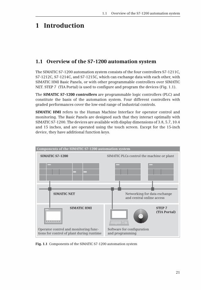
The SIMATIC S7-1200 automation system consists of the four controllers S7-1211C,S7-1212C, S7-1214C, and S7-1215C, which can exchange data with each other, withSIMATIC HMI Basic Panels, or with other programmable controllers over SIMATICNET. STEP 7 (TIA Portal) is used to configure and program the devices (Fig. 1.1).
The SIMATIC S7-1200 controllers are programmable logic controllers (PLC) andconstitute the basis of the automation system. Four different controllers withgraded performances cover the low-end range of industrial controls.
SIMATIC HMI refers to the Human Machine Interface for operator control andmonitoring. The Basic Panels are designed such that they interact optimally withSIMATIC S7-1200. The devices are available with display dimensions of 3.8, 5.7, 10.4and 15 inches, and are operated using the touch screen. Except for the 15-inchdevice, they have additional function keys.
Fig. 1.1 Components of the SIMATIC S7-1200 automation system
SIMATIC NET
SIMATIC HMI STEP 7(TIA Portal)
SIMATIC S7-1200
Software for configuration and programming
SS
S S S
Components of the SIMATIC S7-1200 automation system
SIMATIC PLCs control the machine or plant
Networking for data exchange and central online access
Operator control and monitoring func-tions for control of plant during runtime
1 Introduction
22
SIMATIC NET links all SIMATIC stations, and allows trouble-free data exchange.SIMATIC S7-1200 with PROFINET interface uses the Industrial Ethernet network toexchange data with other PLC stations, HMI stations, and programming devices.Communication modules expand the communication capabilities to other net-works such as PROFIBUS DP, AS-Interface, or point-to-point coupling based onRS232 or RS485.
The STEP 7 programming software provides the nesting function for Totally Inte-grated Automation (TIA), the automation system with uniform configuration andprogramming, data management, and data transfer. STEP 7 is used to configureand parameterize the SIMATIC components, and STEP 7 is also used to generate anddebug the user program. The TIA Portal is the central user interface for manage-ment of the tools and automation data. STEP 7 in the TIA Portal is available in theversions STEP 7 Professional and STEP 7 Basic. Both versions can be used to config-ure and program an S7-1200 station. This book describes the use of STEP 7 Basic.
1.1.1 SIMATIC S7-1200
SIMATIC S7-1200 is the modular microsystem for the lower and medium perfor-mance range. The central processing unit (CPU) contains the operating systemand the user program. The user program is located in the load memory and ispower failure-proof. The parts of the user program relevant to execution are pro-cessed in a work memory with fast access. Tags whose values are to be retained inthe event of a power failure or when switching off/on are stored in the retentivememory (Fig. 1.2).
The user program can be transferred to the CPU using a plug-in memory card (MC)– as an alternative to transfer via an online connection to the programming device.The memory card can also be used as an external load memory or for updating thefirmware.
The connections to the plant or process are made by onboard inputs and outputs,their number being determined by the CPU version. The onboard inputs and out-puts are designed especially for operation of the integral high-speed counters(HSC). The operating system additionally includes pulse generators with a pulse-width modulated output and also the technology objects Axis for controlling step-per motors and servo motors with pulse interface and PID Compact, a PID controllerwith optimized self-tuning.
A signal board (SB) can be used to expand the onboard inputs and outputs. Thecommunication board (CB) creates a point-to-point connection for the CPU and thebattery board (BB) increases the power reserve of the integrated hardware clock toabout one year.
If further inputs and outputs are required, signal modules (SM) can be pluggedonto the CPU depending on its version. These are available for digital and analogsignals.
The PROFINET interface connects the CPU to the Industrial Ethernet subnet. Theprogramming device is connected to this interface if, for example, the user pro-
1.1 Overview of the S7-1200 automation system
23
gram is to be transferred online to the CPU and tested on the machine. Data isexchanged with HMI stations and other automation devices via this interface.
If the CPU is only connected to one device over Ethernet, a standard or crossovercable can be used. If more than two devices that only have a PROFINET interface arenetworked, the connecting cables must be routed via a multiplier, e.g. the commu-nication switch module (CSM). A CPU 1215 has two ports connected with a switchso that they can be networked with the next programmable controller without aninterposed connection multiplier.
Communication modules (CM) permit the operation on further bus systems suchas PROFIBUS DP. Here, an S7-1200 station in a DP master system can be both DPmaster and DP slave. An S7-1200 station can be the AS-Interface master on AS-Inter-face and can control up to 62 AS-Interface field devices. The communication mod-ule for the point-to-point connection is available with RS232 or RS485 interface, towhich, for example, a barcode or RFID reader can be connected.
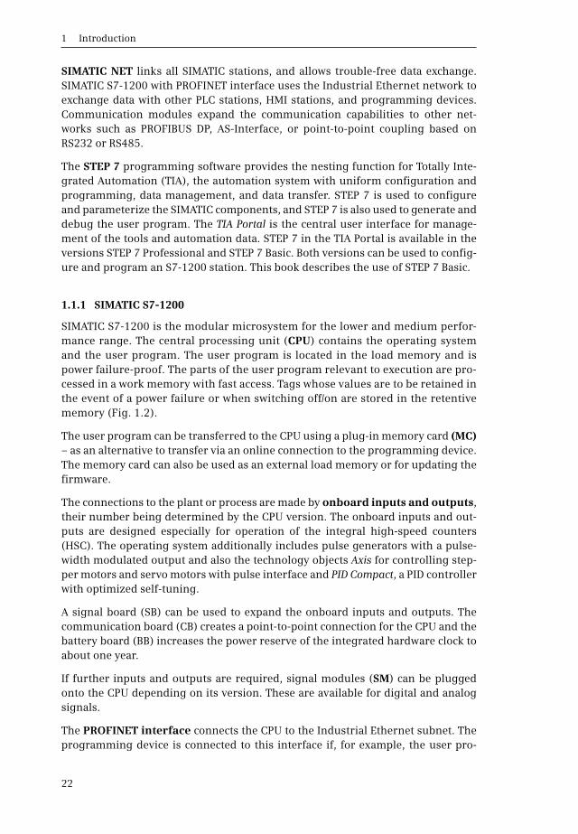
Fig. 1.2 Connection options to a PLC station with CPU 1200
S
Connection options to a CPU 1200
Connection of an HMI station (Basic Panel).
Multiplication of Ethernet connec-tion using the communication switch module (CSM).
Connection of sensors, e.g. buttons or limit switches, to the onboard I/O, to the signal board (SB) or to a signal module (SM).
Connection of a further S7-1200 station or other devices on the basis of open user communication.
A memory card (MC) can be used to transfer the control program and upgrade the operating system.
Connection of a programming device.
Connection of devices using communication modules (CM) with RS232 and RS485.
Connection of actuators, e.g. contactors or lamps, to the onboard I/O, to the signal board (SB) or to a signal module (SM).
1 Introduction
24
1.1.2 Overview of STEP 7 Basic
STEP 7 is the central automation tool for SIMATIC. STEP 7 requires authorization(licensing), and is executed on the current Microsoft Windows operating systems.STEP 7 Basic can be used to configure the S7-1200 controllers and – with WinCCBasic – the Basic Panels. Configuration is carried out in two views: the Portal viewand the Project view.
The Portal view is task-oriented.
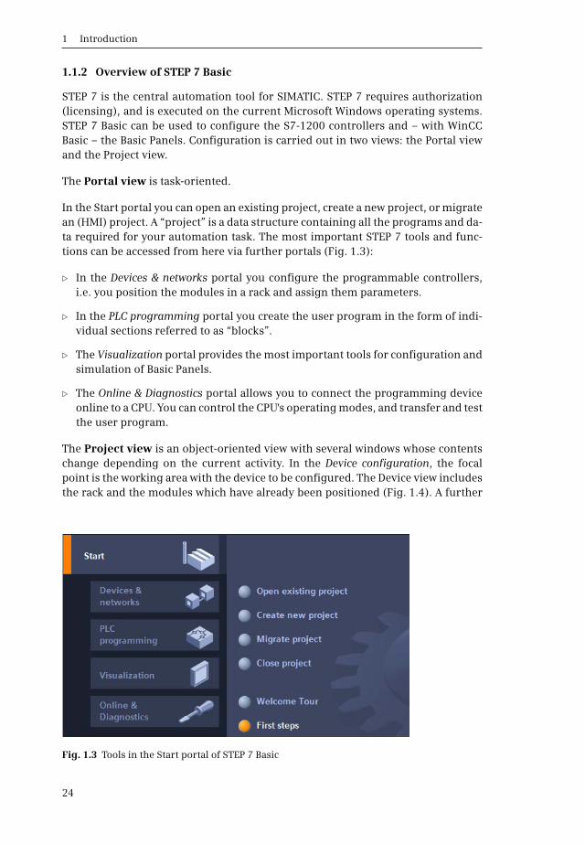
In the Start portal you can open an existing project, create a new project, or migratean (HMI) project. A “project” is a data structure containing all the programs and da-ta required for your automation task. The most important STEP 7 tools and func-tions can be accessed from here via further portals (Fig. 1.3):
b In the Devices & networks portal you configure the programmable controllers,i.e. you position the modules in a rack and assign them parameters.
b In the PLC programming portal you create the user program in the form of indi-vidual sections referred to as “blocks”.
b The Visualization portal provides the most important tools for configuration andsimulation of Basic Panels.
b The Online & Diagnostics portal allows you to connect the programming deviceonline to a CPU. You can control the CPU's operating modes, and transfer and testthe user program.
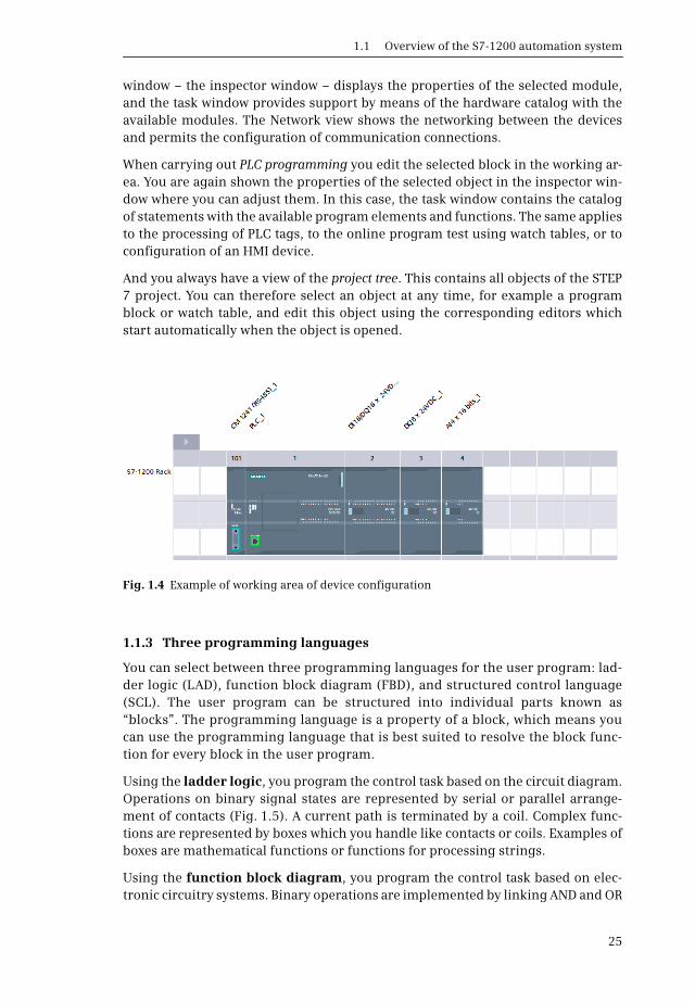
The Project view is an object-oriented view with several windows whose contentschange depending on the current activity. In the Device configuration, the focalpoint is the working area with the device to be configured. The Device view includesthe rack and the modules which have already been positioned (Fig. 1.4). A further
Fig. 1.3 Tools in the Start portal of STEP 7 Basic
1.1 Overview of the S7-1200 automation system
25
window – the inspector window – displays the properties of the selected module,and the task window provides support by means of the hardware catalog with theavailable modules. The Network view shows the networking between the devicesand permits the configuration of communication connections.
When carrying out PLC programming you edit the selected block in the working ar-ea. You are again shown the properties of the selected object in the inspector win-dow where you can adjust them. In this case, the task window contains the catalogof statements with the available program elements and functions. The same appliesto the processing of PLC tags, to the online program test using watch tables, or toconfiguration of an HMI device.
And you always have a view of the project tree. This contains all objects of the STEP7 project. You can therefore select an object at any time, for example a programblock or watch table, and edit this object using the corresponding editors whichstart automatically when the object is opened.
1.1.3 Three programming languages
You can select between three programming languages for the user program: lad-der logic (LAD), function block diagram (FBD), and structured control language(SCL). The user program can be structured into individual parts known as“blocks”. The programming language is a property of a block, which means youcan use the programming language that is best suited to resolve the block func-tion for every block in the user program.
Using the ladder logic, you program the control task based on the circuit diagram.Operations on binary signal states are represented by serial or parallel arrange-ment of contacts (Fig. 1.5). A current path is terminated by a coil. Complex func-tions are represented by boxes which you handle like contacts or coils. Examples ofboxes are mathematical functions or functions for processing strings.
Using the function block diagram, you program the control task based on elec-tronic circuitry systems. Binary operations are implemented by linking AND and OR
Fig. 1.4 Example of working area of device configuration

1 Introduction
26
functions and terminated by simple boxes (Fig. 1.6). Complex boxes are used tohandle the operations on digital tags, for example with mathematical functions orfunctions for strings.
Structured control language is particularly suitable for programming complexalgorithms or for tasks in the area of data management. The program is made up ofSCL statements which, for example, can be value assignments, comparisons, orcontrol statements (Fig. 1.7).
Fig. 1.5 Example of binary operations in ladder logic representation
Fig. 1.6 Example of binary operations in function block diagram representation
Fig. 1.7 Example of SCL statements
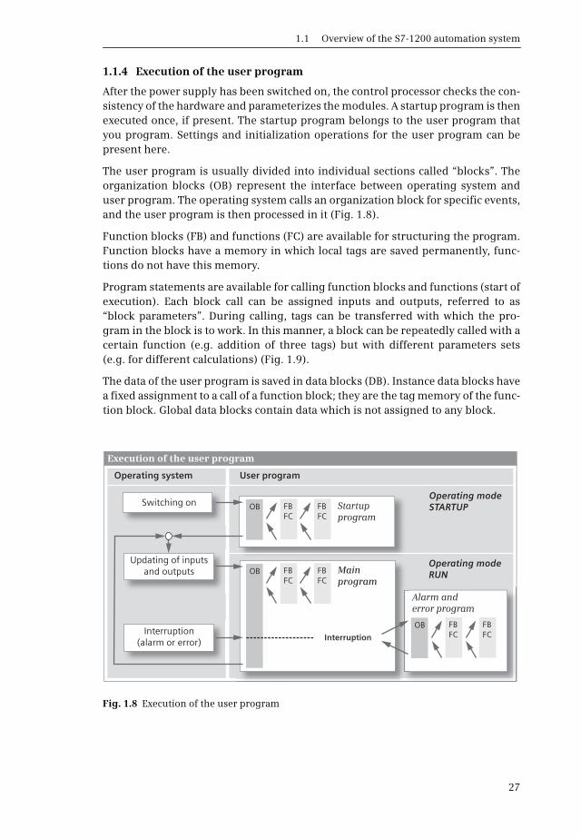
1.1 Overview of the S7-1200 automation system
27
1.1.4 Execution of the user program
After the power supply has been switched on, the control processor checks the con-sistency of the hardware and parameterizes the modules. A startup program is thenexecuted once, if present. The startup program belongs to the user program thatyou program. Settings and initialization operations for the user program can bepresent here.
The user program is usually divided into individual sections called “blocks”. Theorganization blocks (OB) represent the interface between operating system anduser program. The operating system calls an organization block for specific events,and the user program is then processed in it (Fig. 1.8).
Function blocks (FB) and functions (FC) are available for structuring the program.Function blocks have a memory in which local tags are saved permanently, func-tions do not have this memory.
Program statements are available for calling function blocks and functions (start ofexecution). Each block call can be assigned inputs and outputs, referred to as“block parameters”. During calling, tags can be transferred with which the pro-gram in the block is to work. In this manner, a block can be repeatedly called with acertain function (e.g. addition of three tags) but with different parameters sets(e.g. for different calculations) (Fig. 1.9).
The data of the user program is saved in data blocks (DB). Instance data blocks havea fixed assignment to a call of a function block; they are the tag memory of the func-tion block. Global data blocks contain data which is not assigned to any block.
Fig. 1.8 Execution of the user program
Startup program
Alarm and error program
Main program
Execution of the user program
Switching on
Updating of inputsand outputs
Interruption(alarm or error)
Operating modeSTARTUP
Operating system User program
Operating modeRUN
OB
OB
FBFC
FBFC
FBFC
FBFC
FBFC
FBFC
OB
Interruption
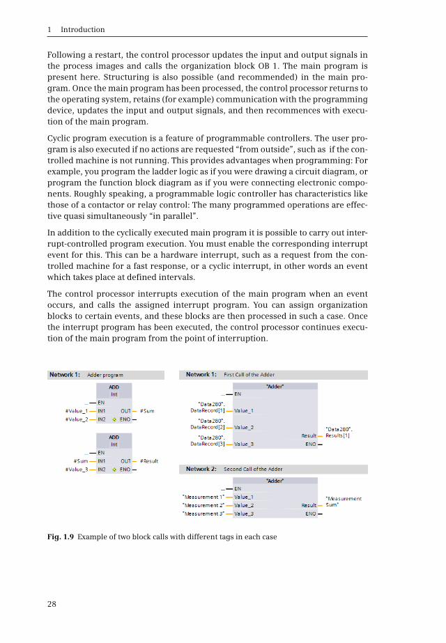
1 Introduction
28
Following a restart, the control processor updates the input and output signals inthe process images and calls the organization block OB 1. The main program ispresent here. Structuring is also possible (and recommended) in the main pro-gram. Once the main program has been processed, the control processor returns tothe operating system, retains (for example) communication with the programmingdevice, updates the input and output signals, and then recommences with execu-tion of the main program.
Cyclic program execution is a feature of programmable controllers. The user pro-gram is also executed if no actions are requested “from outside”, such as if the con-trolled machine is not running. This provides advantages when programming: Forexample, you program the ladder logic as if you were drawing a circuit diagram, orprogram the function block diagram as if you were connecting electronic compo-nents. Roughly speaking, a programmable logic controller has characteristics likethose of a contactor or relay control: The many programmed operations are effec-tive quasi simultaneously “in parallel”.
In addition to the cyclically executed main program it is possible to carry out inter-rupt-controlled program execution. You must enable the corresponding interruptevent for this. This can be a hardware interrupt, such as a request from the con-trolled machine for a fast response, or a cyclic interrupt, in other words an eventwhich takes place at defined intervals.
The control processor interrupts execution of the main program when an eventoccurs, and calls the assigned interrupt program. You can assign organizationblocks to certain events, and these blocks are then processed in such a case. Oncethe interrupt program has been executed, the control processor continues execu-tion of the main program from the point of interruption.
Fig. 1.9 Example of two block calls with different tags in each case

1.1 Overview of the S7-1200 automation system
29
1.1.5 Data management in the SIMATIC automation system
The automation data is present in various memory locations in the automation sys-tem. Initially there is the programming device, referred to generally as the genera-tion or engineering system. All automation data of a STEP 7 project is saved on itshard disk. Configuration and programming of the project data with STEP 7 is car-ried out in the main memory of the programming device (Fig. 1.10).
The automation data on the hard disk is also referred to as the offline project data.Once STEP 7 has appropriately compiled the automation data, this can bedown-loaded to a programmable controller. The data downloaded into the usermemory of the CPU module are known as the online project data.
The user memory on the CPU is divided into three components: The load memorycontains the complete user program including the configuration data, the workmemory contains the executable user program with the current control data, andthe retentive memory contains the tags whose current values are saved power-fail-ure-proof.
The memory card as a transfer card can transfer the user program to the CPU mem-ory, or as a program card expand the CPU's internal load memory. When used as aprogram card, the memory card remains inserted in the CPU during runtime.
Fig. 1.10 Data management in the SIMATIC automation system
Memory card
Work memoryRetentive memory
Main memory
Hard disk
Load memory
The load memory containsthe project data transferred
to the CPU. Togetherwith the current values of
the tags from the workmemory, they form the
online project data.The control programcan be transferred tothe CPU by means of
the memory card.
The work memorycontains the executable
part of the control programwhich is processed
during runtime.
The retentive memorycontains the tags whose
values are retained in theevent of a power failure
or when switching off/on.
The offline projectdata is saved on
the hard disk.
All project datais executed in the
programming device's main memory.
Programming device CPU module
Transfer whenswitching on
Saving theproject data
Data management in the SIMATIC automation system
Transfer with online connection

1 Introduction
30
1.1.6 Operator control and monitoring with process images
Procedures in the process (on the controlled machine) are manually controlled andmonitored using an HMI device. With the Basic Panels, a touch screen permits ac-cess using control elements represented on the monitor. Control and display ele-ments are combined in process images. A process image can map a plant, displayprocess sequences, output process values, or permit operator actions (Fig. 1.11).
The image sequence has a hierarchical structure. Commencing with a start screenwhich is displayed when the HMI device is switched on, it is possible to select thescreens of the next level, from where the screens of the following level can beselected, and so on. Displays can be changed manually using key or touch inputs, ortriggered by the user program.
Predefined objects are available for creating a screen, and can be inserted andadapted according to your requirements. These can be static objects such as text orgraphics which do not change during process operation, or dynamic objects suchas texts, numerical values, trends and bar charts which change depending on pro-cess values.
The functional scope of the Basic Panels also includes message control with bit andanalog messages, management of recipes, and user administration.
Fig. 1.11 Example of a process image in the configuration stage
1.2 Introduction to STEP 7 Basic for S7-1200
31
1.2 Introduction to STEP 7 Basic for S7-1200
1.2.1 Installing STEP 7
STEP 7 Basic V11 is a 32-bit applica-tion, which executes with MS Win-dows XP (Home with SP3 or Profes-sional with SP3) or MS Windows 7(Home Premium, Professional, Enter-prise, or Ultimate, 32/64-bit). Yourequire administration rights inorder to install STEP 7, and to workwith STEP 7 you must at least belogged-on as a main user.
The processor should at least be a Pentium 4 with 1.7 GHz or a comparable type.A main memory of 1 GB is required for working with Windows XP, and should be2 GB for Windows Vista. STEP 7 Basic requires approx. 2 GB on the hard disk.
An Ethernet interface (LAN adapter) is required on the programming device for theonline connection to a programmable controller or Basic Panel. If you wish to workwith a SIMATIC memory card, you require an SD card reader.
Installation is carried out using the setup program start.exe on the DVD. Deinstalla-tion of STEP 7 Basic is carried out as usual in MS Windows using the Software pro-gram in the Windows Control Panel. Parallel online use of STEP 7 Basic and STEP 7has not been enabled.
1.2.2 Automation License Manager
You require a license (user authoriza-tion) in order to use STEP 7. Licensesare managed by the AutomationLicense Manager which is installedtogether with STEP 7 Basic. Thelicense key for STEP 7 Basic is trans-ferred to the hard disk during theinstallation, and removed again fromthe hard disk during deinstallation.
The license key is stored on the hard disk in specially identified blocks. To avoid un-intentional destruction of the license key, you should observe the information forhandling license keys in the Help text of the Automation License Manager.
The Automation License Manager also manages the license keys of other SIMATICproducts, e.g. STEP 7 V5.4 and WinCC.

1 Introduction
32
1.2.3 Starting STEP 7 Basic
You start STEP 7 Basic either using the Start button of Windowsand Programs > Siemens Automation > TIA Portal V11, or by dou-ble-clicking the icon on the Windows desktop. The Totally Inte-grated Automation Portal is the user interface for STEP 7 and mayalso contain other applications which use the same database. Forexample, STEP 7 Basic V11 includes the WinCC Basic configuration software whichis displayed as an integrated “Visualization” editor in the Start portal.
1.2.4 Portal view
Following starting-up, STEP 7 Basic displays the Start portal. A portal makes avail-able all functions and tools required for the respective range of tasks in theportal view. The scope of the portals as well as the range of functions and tools de-pends on the installed applications. The Start portal of STEP 7 Basic permit selectionof the following portals (Fig. 1.12):
b In the Devices & networks portal you can configure the hardware of the program-mable controller, i.e. you select the hardware components, position them, andset their properties. If several devices are networked, you can define the connec-tions here.
b The PLC programming portal contains all the tools required for generating theuser program for a PLC station (programmable logic controller).
Fig. 1.12 Portal view: First steps after opening a project
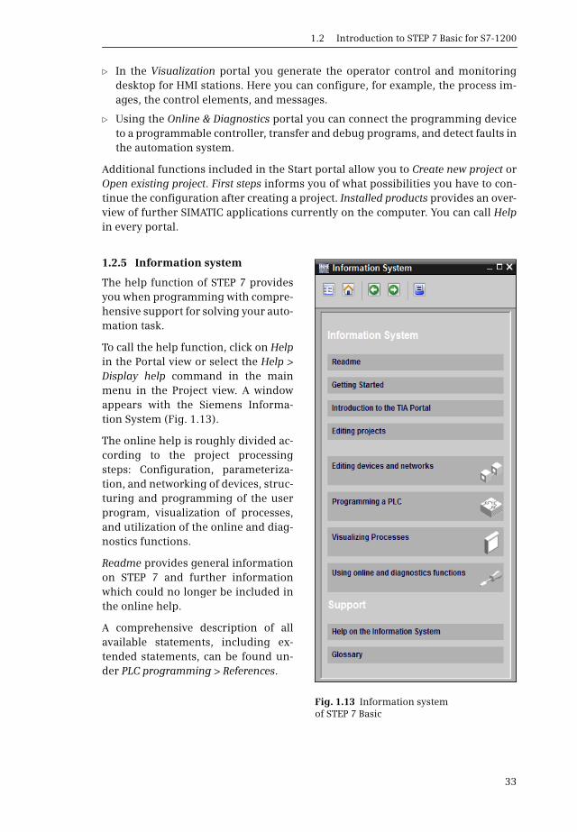
1.2 Introduction to STEP 7 Basic for S7-1200
33
b In the Visualization portal you generate the operator control and monitoringdesktop for HMI stations. Here you can configure, for example, the process im-ages, the control elements, and messages.
b Using the Online & Diagnostics portal you can connect the programming deviceto a programmable controller, transfer and debug programs, and detect faults inthe automation system.
Additional functions included in the Start portal allow you to Create new project orOpen existing project. First steps informs you of what possibilities you have to con-tinue the configuration after creating a project. Installed products provides an over-view of further SIMATIC applications currently on the computer. You can call Helpin every portal.
1.2.5 Information system
The help function of STEP 7 providesyou when programming with compre-hensive support for solving your auto-mation task.
To call the help function, click on Helpin the Portal view or select the Help >Display help command in the mainmenu in the Project view. A windowappears with the Siemens Informa-tion System (Fig. 1.13).
The online help is roughly divided ac-cording to the project processingsteps: Configuration, parameteriza-tion, and networking of devices, struc-turing and programming of the userprogram, visualization of processes,and utilization of the online and diag-nostics functions.
Readme provides general informationon STEP 7 and further informationwhich could no longer be included inthe online help.
A comprehensive description of allavailable statements, including ex-tended statements, can be found un-der PLC programming > References.
Fig. 1.13 Information system of STEP 7 Basic
1 Introduction
34
1.2.6 The windows of the project view
The project view shows all elements of a project in structured form in various pro-cessing windows. You can move from the Portal view to the Project view using theProject view link at the bottom left of the screen, or STEP 7 automatically switches tothe Project view depending on the selected tool.
Fig. 1.14 shows the windows of the Project view in an example of block program-ming. Different window contents are displayed depending on the currently usededitor.
a Main menu and toolbar, shortcut menu
Underneath the title bar is the main menu with all menu commands. The menucommands available for selection depend on the currently marked object; menucommands which cannot be selected are displayed in gray. The same functionalityis available – somewhat user-friendlier – with the shortcut menu: if you click on anobject with the right mouse button, a window is opened with the currently select-able menu commands. Underneath the main menu is the toolbar with the graphi-cally represented “main functions”. The main menu and the toolbar are alwayspresent in all editors.
Using Options > Customize in the main menu you can adapt the user interface.For example, under “General” you can define the interface language in whichSTEP 7 is used, and the mnemonics (the representation of the operands: “I” for in-put (international), or “E” in German).
s Working window
In the center of the screen is the working window. The contents of the working win-dow depend on the editor currently being used. In the case of device configuration,the working window is divided in two: the objects (modules and stations) are dis-played in graphic form in the top part, and in tabular form in the bottom part. Whenprogramming the PLC, the top part of the working window contains the interfacedescription of the block, and the bottom part the program represented in LAD, FBD,or SCL. You use the working window to configure the hardware of the automationsystem, generate the user program, or configure the process screens for HMIdevices.
You can separate the working window completely from the project view so that it isdisplayed as a separate window (“Release” icon in the title bar of the working win-dow), and also insert it again (“Embed” icon). The “Maximize” icon closes all otherwindows and displays the working window in maximum size.
d Inspector window
The inspector window underneath the working window shows the properties of theobjects marked in the latter, records the sequence of actions, and provides an over-view of the diagnostics status of the connected devices.
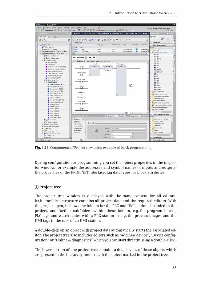
1.2 Introduction to STEP 7 Basic for S7-1200
35
During configuration or programming you set the object properties in the inspec-tor window, for example the addresses and symbol names of inputs and outputs,the properties of the PROFINET interface, tag data types, or block attributes.
f Project tree
The project tree window is displayed with the same content for all editors.Its hierarchical structure contains all project data and the required editors. Withthe project open, it shows the folders for the PLC and HMI stations included in theproject, and further subfolders within these folders, e.g. for program blocks,PLC tags and watch tables with a PLC station or e.g. the process images and theHMI tags in the case of an HMI station.
A double-click on an object with project data automatically starts the associated ed-itor. The project tree also includes editors such as “Add new device”, “Device config-uration” or “Online & diagnostics” which you can start directly using a double-click.
The lower section of the project tree contains a details view of those objects whichare present in the hierarchy underneath the object marked in the project tree.
Fig. 1.14 Components of Project view using example of block programming

1 Introduction
36
g Task window
To the right of the working window is the task window with the task cards. This con-tains further objects for processing in the working window. The contents of the taskwindow depend on the currently active editor. In the case of the hardware configu-ration, for example the hardware catalog with the available components is shownhere, in the case of PLC programming the program elements catalog appears, withonline & diagnostics the online tools, and with the visualization the library for theprocess image control and display elements.
You can also call the libraries in this window: global libraries supplied with STEP 7,or the project library in which you can save reusable objects such as programblocks, templates for process images, or control elements with special configura-tions.
h Editor and status bar
At the bottom left of the Project view you can change to the Portal view. In the mid-dle you can see the tabs of the open windows. Clicking on a tab results in its contentsbeing displayed in the top level of the working window. This makes it easy to changequickly between different window contents. The far right of the status bar indicatesthe current status of project processing.
1.2.7 Adapting the user interface
The language of the user interface can be changed. In the main menu selectOptions > Settings and the “General” section. In the “Interface language” drop-downlist you can select the desired language from the installed languages. The texts ofthe user interface are then immediately displayed in the new language. You can alsodefine here how the TIA Portal is to be displayed following the next restart.
You can show or hide the displayed window using the menu item View. You can al-ways change the size of windows by dragging on the edge with the mouse. Windowscan be minimized into a symbol which appears in one of the navigation bars in theleft, bottom or right margin of the screen.
You can maximize the working window, or release it from the windows group anddisplay it as a separate window. The working window can be divided vertically orhorizontally, permitting you to view two working areas simultaneously.
You can change the width of table columns by dragging with the cursor in the tableheader. In the case of columns that are too narrow, the entire content of the individ-ual cells will appear as a tooltip when the cursor is briefly hovered over the relevantfield.

1.3 Editing a SIMATIC project
37
1.3 Editing a SIMATIC project
Fig. 1.15 shows all tools and data which can be of importance in an automation task.Of prime importance is the Project which contains all the automation data requiredfor control and operation of the machine or plant. The project data is roughly divid-ed into the data for the individual stations and the common project data which ap-plies to all stations in the project.
A station can be a controller (PLC station) or an HMI device (HMI station). A projectcan include several stations, but at least one station must be present. The data pres-ent in a station is described further below. Common Project Data includes, for exam-ple, centrally managed message texts or texts for multilingual projects.
A project library is created for each project. Objects which are used in several proj-ects are combined in global libraries. Also relevant to a project is the programmingdevice design with interface modules (LAN adapters) and SD card readers.
Fig. 1.15 Project components, libraries and programming device design
Global Libraries
System Libraries
User Libraries
HMI Buttons-and-Switches
Online access
< User Library >
< Project Library >
Monitoring-and-control-objects
SIMATIC Card Reader
Documentation templates
Libraries delivered with STEP 7.
Libraries configured by users themselves.
Contains the programming device resources relevant to the project.
Contains all the data for a controller.
Contains text lists for system and user messages.
Contains all the data for an HMI device.
Contains document info, frames and cover sheets
PLC station
Common Data
HMI station
Documentation settings
Contains project texts, project languages and graphics.Languages & resources
Stations
Project
Common Project Data
Project Library
All the data for the automation task is combined in a project.
Stations can be controllers (PLC stations) or HMI devices (HMI stations). A project includes at least one station.
Contains cross-station data.
Contains cross-station data compiled by the user.
Global libraries contain elements for multiple use across projects.
Programming Device Design
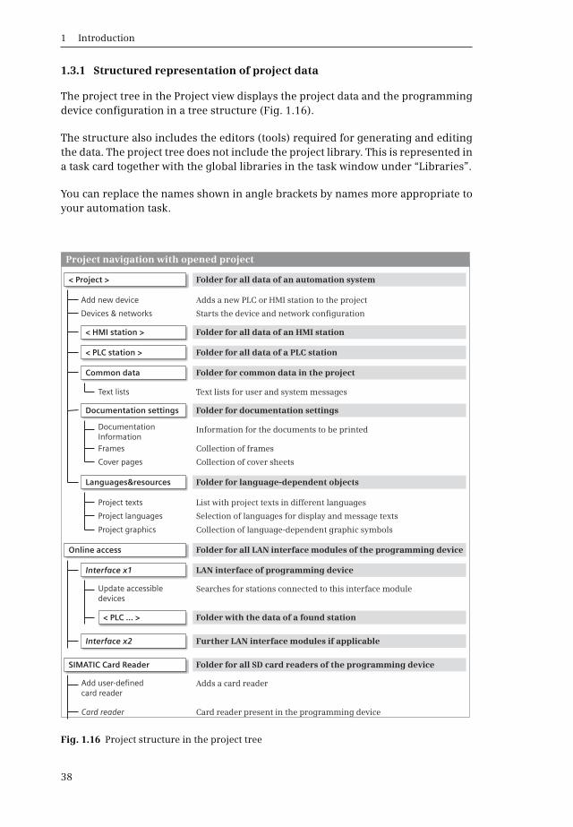
1 Introduction
38
1.3.1 Structured representation of project data
The project tree in the Project view displays the project data and the programmingdevice configuration in a tree structure (Fig. 1.16).
The structure also includes the editors (tools) required for generating and editingthe data. The project tree does not include the project library. This is represented ina task card together with the global libraries in the task window under “Libraries”.
You can replace the names shown in angle brackets by names more appropriate toyour automation task.
Fig. 1.16 Project structure in the project tree
< Project >
Online access
SIMATIC Card Reader
< HMI station >
Interface x1
< PLC station >
Common data
Interface x2
< PLC ... >
Languages&resources
Documentation settings
Add new device
Text lists
Project texts
Documentation Information
Project languages
Frames
Project graphics
Cover pages
Devices & networks
Update accessible devices
Add user-defined card reader
Card reader
Adds a new PLC or HMI station to the project
Folder with the data of a found station
Text lists for user and system messages
List with project texts in different languages
Information for the documents to be printed
Selection of languages for display and message texts
Collection of frames
Collection of language-dependent graphic symbols
Collection of cover sheets
Starts the device and network configuration
Searches for stations connected to this interface module
Adds a card reader
Card reader present in the programming device
Folder for all data of an automation system
Folder for all LAN interface modules of the programming device
Folder for all SD card readers of the programming device
Folder for all data of an HMI station
LAN interface of programming device
Folder for all data of a PLC station
Folder for common data in the project
Further LAN interface modules if applicable
Folder for language-dependent objects
Folder for documentation settings
Project navigation with opened project

1.3 Editing a SIMATIC project
39
1.3.2 Project data and editors for a PLC station
If you add a PLC station (an S7-1200 controller) to the project, STEP 7 creates thecorresponding structure in the project data (Fig. 1.17). A PLC or HMI station isalways required for editing in a project so that STEP 7 can create the data structuresrequired for the PLC programming or HMI configuration. If you wish to write a userprogram without previously selecting a specific CPU, you can select an “unspecifiedCPU” from the hardware catalog and replace it later with a “real” CPU 1200 if nec-essary.
Fig. 1.17 Structure of the project data for a PLC station
< PLC_12xxC >
Program blocks *)
Watch and force tables *)
PLC data types *)
Local modules
Technology objects
External source files *)
PLC tags *)
< Technology object_1 >
<Source file_1>
Device configuration
Add new block
Add new watch table
Add new data type
PLC_DataType_1
Add new object
Add new external file
Show all tags
Add new tag table
Default tag table [n]
Tag table_1 [m]
Online & diagnostics
< Block_1 >
Force table
< Watch table_1 >
Text lists
Program info
Starts the editor for the device configuration
Creates a new block and opens it
Main program (organization block OB 1)
Self-created block
Creates a new watch table and opens it
Creates a new PLC data type
Self-created PLC data type
Table with the forced tags
Self-created watch table
Station-specific texts for user and system alarms
Program structure, assignment list, memory utilization
Creates a new technology object and opens it
Imports a new source file
Displays the tags of all (sub-)tables
Adds a new tag table
Permanently available tag table with n tags
Self-created tag table with m tags
Starts the editor for the online connection and diagnostics
Folder for all data of a PLC station (name can be freely-selected)
Folder for all blocks of the user program
Folder for the force table and all watch tables
Folder for all PLC data types
Folder for the local modules of the PLC station
Folder for all technology objects
Folder for external source files (SCL)
Folder for all PLC tags (“symbol table”)
Self-created technology object
Imported source file
Data structure of a PLC station
*) Sub-groups can be generated
Main [OB 1]
1 Introduction
40
The user program which controls the machine or process is located in the Programblocks folder. The program comprises blocks (separate program components)which are either stored directly in the Program blocks folder or – if there is a largenumber – in subfolders which you can create and configure yourself. The “Main”block (the name is the symbol for the block and can be changed) is the organizationblock OB 1 and is created automatically. The processing sequence of the blocks isdefined in the user program by “block calls” and is displayed by opening the Pro-gram information object under Call structure.
The Technology objects folder contains the configuration data for the motion con-trol objects (axes) and control loop objects (PID controllers).
SCL source files can be saved in the External sources files folder.
The PLC tags folder contains the assignment of the absolute address to the symbolicaddress of global tags that are valid throughout the PLC station (inputs, outputs,and bit memories).
The PLC data types folder contains user-defined, structured data types.
The force table and all created watch tables can be found in the Watch and forcetables folder. A watch table is used during testing of the user program. It containstags whose current value can be monitored and also changed during runtime. Theforce tables can be used to set tags to fixed values that cannot be changed by theprogram.
The program information shows the program structure (sequence and dependen-cies of the block calls), the assignment list for inputs, outputs and bit memories,and the memory usage.
Message texts are stored under Text lists. In the case of the user-defined text list, youcan specify the value ranges which trigger the messages and the associated texts;with a system-defined text list, the contents are specified by STEP 7. Text lists creat-ed under a PLC station contain station-specific texts, those created under a projectcontain cross-station texts.
The Local modules folder contains all configured modules of the PLC station. Open-ing a module initiates device configuration. The module properties are displayed inthe inspector window.
You start configuration of a station using the Device configuration editor which islocated in the first position in the project structure. There is no correspondingfolder for the data of the device configuration in the project tree. The configurationdata is located “behind” the Device configuration editor.
Online & diagnostics starts the editor for the online connection and online func-tions. For example, you can use a (software) control panel to control the operatingmodes of the CPU, to set the CPU's IP address and time, or read the CPU's diagnosticsbuffer.

1.3 Editing a SIMATIC project
41
1.3.3 Creating and editing a project
Creating a new project
You can create a new project in the Portal view if you click in the Start portal onCreate new project. Assign a name to the project and set a path in which the projectis to be saved. After clicking the Create button, any project which is open is closed,the new project is created, and the next steps displayed in the Start portal for selec-tion:
b Configure a deviceSTEP 7 changes to the Devices & networks portal in which you can insert a newCPU 1200 (a PLC station) into the project and open it for editing.
b Write PLC programSTEP 7 changes to the PLC programming portal in which you can edit the “Main”block (organization block OB 1) or insert a new block and open it for editing. APLC station must first have been added to the project.
b Configure an HMI screenSTEP 7 changes to the Visualization portal in which you can create a new HMI sta-tion or configure an already existing one. From this portal you start configura-tion of the process images, editing of HMI tags and messages, and the simulator.
b Open the project viewSTEP 7 changes to the Project view in which you can carry out the next steps(insert and configure PLC stations, insert and program blocks, or insert and con-figure HMI stations).
In the project tree you can create a new project using the Project > New menu com-mand. Assign a name to the project in the dialog window, set the path in which theproject is to be saved, and click on the “Create” button.
Editing an existing project
You can open an existing project in either the Portal view or the Project view. Eitheractivate Open existing project in the Portal view or Project > Open in the Project view.Select the desired project from the list of projects last used. Any project which isopen is closed, and the selected project is opened.
During editing in the Project view, you can save the entered project data using theProject > Save or Project > Save as menu command. You can close the project usingProject > Close – following confirmation of whether changes are to be saved – with-out exiting STEP 7.
You can delete a (closed) project from the hard disk – following confirmation –using Project > Delete.
Compiling and downloading project data
Before project data can be downloaded to a station, it must be made readable for theprocessor: it must be “compiled”. The project data is compiled station-by-station.
1 Introduction
42
The scope of the compilation can be varied depending on the type of station. For ex-ample, the command from the Compile > Software pop-up menu only compilesthose software components which have been changed since the last compilation.
Printing project data
The project data can be printed in the form of a circuit manual. You can use thedocumentation function to set the layout of the printout. Under Document settingsin the project tree, you adapt the existing template or create a new template, forexample in the sizes A3 or A4 in portrait or landscape format. You complete the textfields under Document information (e.g. the title block). You can also position newtext fields or graphic symbols in the layout.
By means of the print preview or print output, you can specify the output with orwithout cover page and as compact (abbreviated) or complete.
Converting a project from STEP 7 V10.5 to STEP V11
To convert a project created with STEP 7 V10.5, start STEP 7 V11 and select Project >Open from the main menu. In the dialog window, click on the Browse button andselect the desired project from the file directory. In the open project folder, selectthe file <Project_name>.ap10 and click the Open button. Confirm the conversionmessages with OK. The project is converted to Version V11, saved under the name<Project_name>_<STEP7-Version>, and opened. You then compile every station andclear any displayed faults and warnings.
1.3.4 Creating and editing libraries
Libraries are used to save reusable program components. These could include sta-tions, blocks, PLC tag tables, process images or picture elements, for example. Aproject library and global libraries are available. The libraries are displayed in atask card of the task window.
A project library which you can fill with objects is automatically created when youcreate a project. You can structure the contents of the project library using folders.A project library is always opened, saved, and closed together with the project.
Components which can be used in multiple projects are saved in global libraries.There are global system libraries which are supplied with STEP 7, and global userlibraries which you create yourself. A global library is opened, saved, and closed in-dependent of the project. If you wish to use a global library simultaneously withother users, the library must be opened as read-only.

2.1 S7-1200 station components
43
2 SIMATIC S7-1200 automation system
2.1 S7-1200 station components
A complete programmable controller including all I/O modules is referred to as a“station”. This also includes distributed I/O modules connected to the CPU via a bussystem. An S7-1200 station comprises at least the CPU. Depending on the version,it has digital and analog input/output channels and can be fitted with additionalinput/output channels using a signal board (SB).
Depending on the type of CPU, up to eight signal modules can be plugged in whichexpand the station by digital and analog input/output channels. A two-tier design ispossible using a 2-meter long extension cable.
The programming device is connected over Industrial Ethernet. Industrial Ethernetcan also be used to connect further SIMATIC stations or HMI devices to the CPU. Upto three communication modules take over the connection to additional bus sys-tems or to a point-to-point link.
Integral technological functions for measuring and counting tasks, closed-loop con-trol, and motion control allow the CPU 1200 to be used in many complex machinecontrols.
The SIMATIC Memory Card can be used to download configuration data, as an exter-nal load memory, or for a firmware update.
Fig. 2.1 S7-1200 station with CPU S7-1214, two SMs (right) and one CM (left)
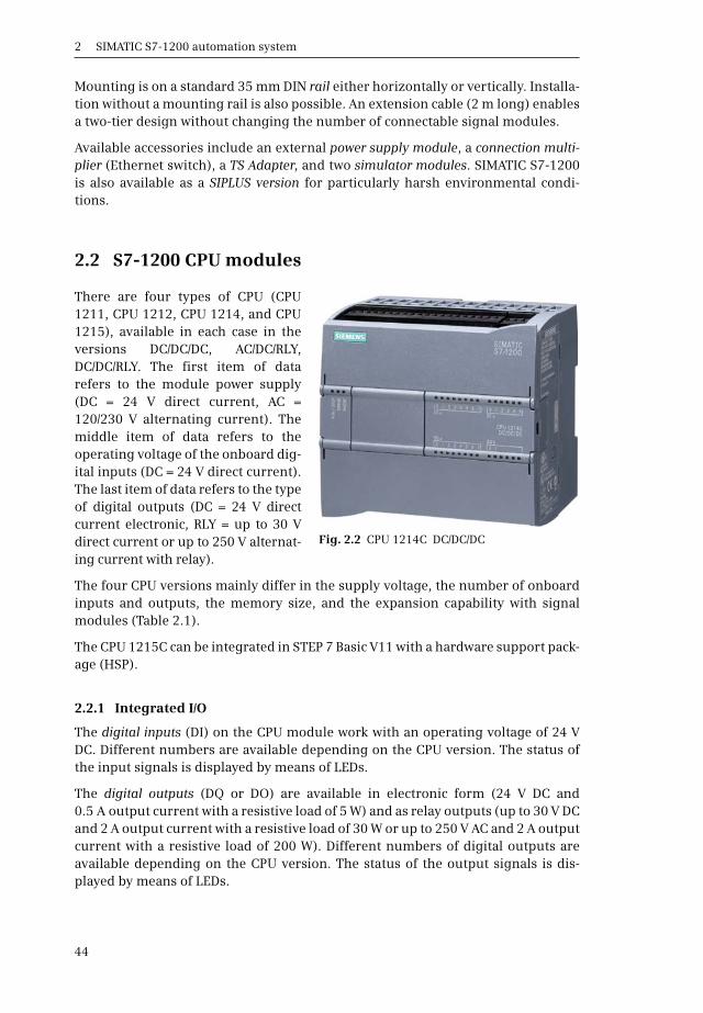
2 SIMATIC S7-1200 automation system
44
Mounting is on a standard 35 mm DIN rail either horizontally or vertically. Installa-tion without a mounting rail is also possible. An extension cable (2 m long) enablesa two-tier design without changing the number of connectable signal modules.
Available accessories include an external power supply module, a connection multi-plier (Ethernet switch), a TS Adapter, and two simulator modules. SIMATIC S7-1200is also available as a SIPLUS version for particularly harsh environmental condi-tions.
2.2 S7-1200 CPU modules
There are four types of CPU (CPU1211, CPU 1212, CPU 1214, and CPU1215), available in each case in theversions DC/DC/DC, AC/DC/RLY,DC/DC/RLY. The first item of datarefers to the module power supply(DC = 24 V direct current, AC =120/230 V alternating current). Themiddle item of data refers to theoperating voltage of the onboard dig-ital inputs (DC = 24 V direct current).The last item of data refers to the typeof digital outputs (DC = 24 V directcurrent electronic, RLY = up to 30 Vdirect current or up to 250 V alternat-ing current with relay).
The four CPU versions mainly differ in the supply voltage, the number of onboardinputs and outputs, the memory size, and the expansion capability with signalmodules (Table 2.1).
The CPU 1215C can be integrated in STEP 7 Basic V11 with a hardware support pack-age (HSP).
2.2.1 Integrated I/O
The digital inputs (DI) on the CPU module work with an operating voltage of 24 VDC. Different numbers are available depending on the CPU version. The status ofthe input signals is displayed by means of LEDs.
The digital outputs (DQ or DO) are available in electronic form (24 V DC and0.5 A output current with a resistive load of 5 W) and as relay outputs (up to 30 V DCand 2 A output current with a resistive load of 30 W or up to 250 V AC and 2 A outputcurrent with a resistive load of 200 W). Different numbers of digital outputs areavailable depending on the CPU version. The status of the output signals is dis-played by means of LEDs.
Fig. 2.2 CPU 1214C DC/DC/DC

2.2 S7-1200 CPU modules
45
Table 2.1 Selected data of a CPU 1200 with Firmware V3.0
CPU 1211C CPU 1212C CPU 1214C CPU 1215C
User memoryInternal load memory *)RAMRetentive memory
1 MB30 KB10 KB
1 MB50 KB10 KB
4 MB75 KB10 KB
4 MB100 KB10 KB
Integrated I/OsDigital inputs (DI)Digital outputs (DO)
6 DI, 24 V DC4 DO, 24 V DC or relay
8 DI, 24 V DC6 DO, 24 V DC or relay
14 DI, 24 V DC10 DO, 24 V DC or relay
14 DI, 24 V DC10 DO, 24 V DC or relay
Analog inputs (AI)Analog outputs (AO)
2 AI (10 bit)–
2 AI (10 bit)–
2 AI (10 bit)–
2 AI (10 bit)2 AO (10 bit)
Process images 1024 bytes inputs, 1024 bytes outputs
Bit memory 4096 bytes 8192 bytes
Expansion with A board (SB, CB, BB) Signal modules (SM) Communication modules (CM)
1None
3
12
3
18
3
18
3
High-speed counteras single-phase counter with integrated I/O
with standard SB with high-speed SB
3 with 100 kHz
2 with 30 kHz2 with 200 kHz
3 with 100 kHz1 with 30 kHz2 with 30 kHz2 with 200 kHz
3 with 100 kHz3 with 30 kHz––
3 with 100 kHz3 with 30 kHz––
as A/B counter with integrated I/O
with standard SB with high-speed SB
3 with 80 kHz
2 with 20 kHz2 with 160 kHz
3 with 80 kHz1 with 20 kHz2 with 20 kHz2 with 160 kHz
3 with 80 kHz3 with 20 kHz––
3 with 80 kHz3 with 20 kHz––
Pulse generators with integrated I/O with standard SB with high-speed SB
4 100 kHz 20 kHz 200 kHz
Pulse outputs **)Inputs for pulse catch
46
48
414
414
Real-time clock buffer Typically 10 days, can be increased up to one year with a battery board
PROFINET connection 1 2 with switch
Temporary local data / nesting depthStartup + main programInterrupt/error processing
16 KB / 16 levels4 KB / 4 levels
Execution time for binary functionsfor digital functionsfor floating-point functions
0.085 µs / instruction1.7 µs / instruction2.3 µs / instruction
*) Expandable up to SD card size**) A digital signal board is required for CPU versions with relay outputs
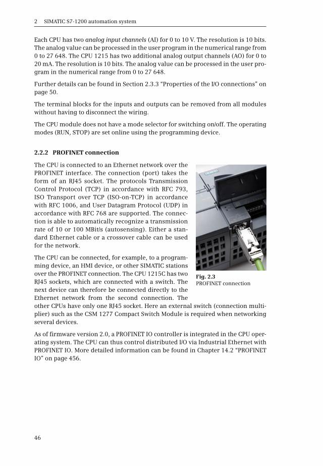
2 SIMATIC S7-1200 automation system
46
Each CPU has two analog input channels (AI) for 0 to 10 V. The resolution is 10 bits.The analog value can be processed in the user program in the numerical range from0 to 27 648. The CPU 1215 has two additional analog output channels (AO) for 0 to20 mA. The resolution is 10 bits. The analog value can be processed in the user pro-gram in the numerical range from 0 to 27 648.
Further details can be found in Section 2.3.3 “Properties of the I/O connections” onpage 50.
The terminal blocks for the inputs and outputs can be removed from all moduleswithout having to disconnect the wiring.
The CPU module does not have a mode selector for switching on/off. The operatingmodes (RUN, STOP) are set online using the programming device.
2.2.2 PROFINET connection
The CPU is connected to an Ethernet network over thePROFINET interface. The connection (port) takes theform of an RJ45 socket. The protocols TransmissionControl Protocol (TCP) in accordance with RFC 793,ISO Transport over TCP (ISO-on-TCP) in accordancewith RFC 1006, and User Datagram Protocol (UDP) inaccordance with RFC 768 are supported. The connec-tion is able to automatically recognize a transmissionrate of 10 or 100 MBit/s (autosensing). Either a stan-dard Ethernet cable or a crossover cable can be usedfor the network.
The CPU can be connected, for example, to a program-ming device, an HMI device, or other SIMATIC stationsover the PROFINET connection. The CPU 1215C has twoRJ45 sockets, which are connected with a switch. Thenext device can therefore be connected directly to theEthernet network from the second connection. Theother CPUs have only one RJ45 socket. Here an external switch (connection multi-plier) such as the CSM 1277 Compact Switch Module is required when networkingseveral devices.
As of firmware version 2.0, a PROFINET IO controller is integrated in the CPU oper-ating system. The CPU can thus control distributed I/O via Industrial Ethernet withPROFINET IO. More detailed information can be found in Chapter 14.2 “PROFINETIO” on page 456.
Fig. 2.3 PROFINET connection
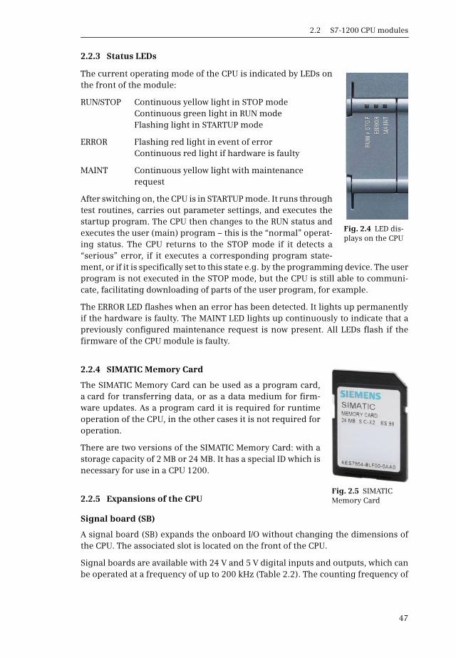
2.2 S7-1200 CPU modules
47
2.2.3 Status LEDs
The current operating mode of the CPU is indicated by LEDs onthe front of the module:
RUN/STOP Continuous yellow light in STOP modeContinuous green light in RUN modeFlashing light in STARTUP mode
ERROR Flashing red light in event of errorContinuous red light if hardware is faulty
MAINT Continuous yellow light with maintenance request
After switching on, the CPU is in STARTUP mode. It runs throughtest routines, carries out parameter settings, and executes thestartup program. The CPU then changes to the RUN status andexecutes the user (main) program – this is the “normal” operat-ing status. The CPU returns to the STOP mode if it detects a“serious” error, if it executes a corresponding program state-ment, or if it is specifically set to this state e.g. by the programming device. The userprogram is not executed in the STOP mode, but the CPU is still able to communi-cate, facilitating downloading of parts of the user program, for example.
The ERROR LED flashes when an error has been detected. It lights up permanentlyif the hardware is faulty. The MAINT LED lights up continuously to indicate that apreviously configured maintenance request is now present. All LEDs flash if thefirmware of the CPU module is faulty.
2.2.4 SIMATIC Memory Card
The SIMATIC Memory Card can be used as a program card,a card for transferring data, or as a data medium for firm-ware updates. As a program card it is required for runtimeoperation of the CPU, in the other cases it is not required foroperation.
There are two versions of the SIMATIC Memory Card: with astorage capacity of 2 MB or 24 MB. It has a special ID which isnecessary for use in a CPU 1200.
2.2.5 Expansions of the CPU
Signal board (SB)
A signal board (SB) expands the onboard I/O without changing the dimensions ofthe CPU. The associated slot is located on the front of the CPU.
Signal boards are available with 24 V and 5 V digital inputs and outputs, which canbe operated at a frequency of up to 200 kHz (Table 2.2). The counting frequency of
Fig. 2.4 LED dis-plays on the CPU
Fig. 2.5 SIMATIC Memory Card
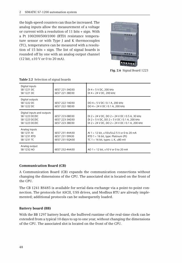
2 SIMATIC S7-1200 automation system
48
the high-speed counters can thus be increased. Theanalog inputs allow the measurement of a voltageor current with a resolution of 11 bits + sign. Witha Pt 100/200/500/1000 (RTD) resistance tempera-ture sensor or with Type J and K thermocouples(TC), temperatures can be measured with a resolu-tion of 15 bits + sign. The list of signal boards isrounded off by one with an analog output channel(12 bit, ±10 V or 0 to 20 mA).
Communication Board (CB)
A Communication Board (CB) expands the communication connections withoutchanging the dimensions of the CPU. The associated slot is located on the front ofthe CPU.
The CB 1241 RS485 is available for serial data exchange via a point-to-point con-nection. The protocols for ASCII, USS drives, and Modbus RTU are already imple-mented; additional protocols can be subsequently loaded.
Battery board (BB)
With the BB 1297 battery board, the buffered runtime of the real-time clock can beextended from a typical 10 days to up to one year, without changing the dimensionsof the CPU. The associated slot is located on the front of the CPU.
Table 2.2 Selection of signal boards
Digital inputsSB 1221 DCSB 1221 DC
6ES7 221-3AD306ES7 221-3BD30
DI 4 5 V DC, 200 kHzDI 4 24 V DC, 200 kHz
Digital outputsSB 1222 DCSB 1222 DC
6ES7 222-1AD306ES7 222-1BD30
DO 4 5 V DC / 0.1 A, 200 kHzDO 4 24 V DC / 0.1 A, 200 kHz
Digital inputs and outputsSB 1223 DC/DCSB 1223 DC/DCSB 1223 DC/DC
6ES7 223-0BD306ES7 223-3AD306ES7 223-3BD30
DI 2 24 V DC, DO 2 24 V DC / 0.5 A, 30 kHzDI 2 5 V DC, DO 2 5 V DC / 0.1 A, 200 kHzDI 2 24 V DC, DO 2 24 V DC / 0.1 A, 200 kHz
Analog inputsSB 1231 AISB 1231 RTDSB 1231 TC
6ES7 231-4HA306ES7 231-5PA306ES7 231-5QA30
AI 1 12 bit, ±10/±5/±2.5 V or 0 to 20 mARTD 1 16 bit, type: Platinum (Pt)TC 1 16 bit, types: J, K, ±80 mV
Analog outputSB 1232 AO 6ES7 232-4HA30 AO 1 12 bit, ±10 V or 0 to 20 mA
Fig. 2.6 Signal Board 1223

2.3 Signal modules (SM)
49
A commercially available CR1025 battery (not included) is used for voltage buffer-ing. The maintenance LED on the board indicates when it is necessary to change thebutton cell.
2.3 Signal modules (SM)
Signal modules are input/output modules which extendthe integrated I/O. Depending on the CPU version, eithernone, two or eight modules can be plugged onto theright of the CPU.
A two-tier design is possible using a 2-meter long exten-sion cable. But the number of modules which can beused is not changed as a result.
2.3.1 Digital I/O modules
Digital modules are signal converters for binary processsignals. The CPU can use input modules to scan operat-ing modes of the machine or plant, and output modulesfor intervention.
Input modules convert external signals of 24 V DC intosignals with an internal level. Output modules convertthe internal signal level into 24 V DC (electronic outputs) or are designed as relayoutputs. Using direct current, a relay can switch maximum 30 W, while with alter-nating current it can switch 200 W. There are signal modules with one or two bytescorresponding to 8 or 16 signals (Table 2.3).
Table 2.3 Selection of digital I/O modules
Digital inputsSM 1221 DCSM 1221 DC
6ES7 221-1BF306ES7 221-1BH30
DI 8 24VDCDI 16 24VDC
Digital outputsSM 1222 DCSM 1222 DCSM 1222 RLYSM 1222 RLYSM 1222 RLY
6ES7 222-1BF306ES7 222-1BH306ES7 222-1HF306ES7 222-1HH306ES7 222 1XF30
DO 8 24VDC / 0.5 ADO 16 24VDC / 0.5 ADO 8 relay 30 V DC, 250 V AC / 2 ADO 16 relay 30 V DC, 250 V AC / 2 ADO 8 relay 30 V DC, 250 V AC / 2 A (change-over contact)
Digital inputs/outputsSM 1223 DC/DCSM 1223 DC/DCSM 1223 DC/RLYSM 1223 DC/RLYSM 1223 AC/RLY
6ES7 223-1BH306ES7 223-1BL306ES7 223-1PH306ES7 223-1PL306ES7 223-1QH30
DI 8 24VDC, DO 8 24VDC / 0.5 ADI 16 24VDC, DO 16 24VDC / 0.5 ADI 8 24VDC, DO 8 relay 30VDC, 250 V AC / 2 ADI 16 24VDC, DO 16 relay 30VDC, 250 V AC / 2 ADI 8 125/250 V AC, DO 8 relay 30 V DC, 250 V AC / 2 A
Fig. 2.7 SM 1221 DI16 signal module

2 SIMATIC S7-1200 automation system
50
2.3.2 Analog input/output modules
Analog modules are signal transducers for analog pro-cess signals. The CPU can use these modules to processanalog variables when these have been converted by an-alog input modules into digital values. The CPU can alsocontinuously supply actuators with analog setpointswhich have been generated from the specified digitalvalues by analog output modules.
One “channel” is occupied on the module by each analogvalue (e.g. measured value or setpoint). Analog modulesare available with 2, 4 or 8 channels corresponding to 4,8 or 16 bytes (Table 2.4). A digitized analog value is rep-resented internally as a 16-bit fixed-point number (datatype INT). Analog modules can output diagnostic dataconcerning the module status or when limit values arereached.
2.3.3 Properties of the I/O connections
Digital input modules convert the external signal voltage (24 V DC or 125/230 VAC) into the internal signal level. The connected sensor must be within the permis-sible voltage range and provide the required input current with the signal status “1”so that the module can switch reliably.
The input signals are filtered in addition, i.e. interferences on the lines are sup-pressed and glitches eliminated. The filtering results in the input signals being de-layed. The input delay can be set. A compromise must be found here between inter-ference resistance (long delay) and fast signal recording (short delay).
Depending on the design, a digital input channel on the CPU module can trigger aprocess interrupt when there is a change in signal status, or be activated as a
Table 2.4 Selection of analog I/O modules
Analog inputsSM 1231 AISM 1231 AISM 1231 AISM 1231 RTDSM 1231 RTDSM 1231 TCSM 1231 TC
6ES7 231-4HD306ES7 231-4HF306ES7 231 5ND306ES7 231-5PD306ES7 231-5PF306ES7 231-5QD306ES7 231-5QF30
AI 4 13 bit, ±10/±5/±2.5 V or 0 to 20 mAAI 8 13 bit, ±10/±5/±2.5 V or 0 to 20 mAAI 4 16 bit, ±10/±5/±2.5/±1.25 V or 0 to 20/4 to 20 mARTD 4 16 bit, 0 to 150/300/600 ; (Pt, Ni, Cu)RTD 8 16 bit, 0 to 150/300/600 ; (Pt, Ni, Cu)TC 4 16 bit, ± 80 mV; types J, K, T, E, R, S, N, C, TXK/XK(L)TC 8 16 bit, ± 80 mV; types J, K, T, E, R, S, N, C, TXK/XK(L)
Analog outputsSM 1232 AOSM 1232 AO
6ES7 232-4HB306ES7 232-4HD30
AO 2 14 bit, ±10 V or 0 to 20 mAAO 4 14 bit, ±10 V or 0 to 20 mA
Analog inputs/outputsSM 1234 AI/AO 6ES7 234-4HE30 AI 4 13 bit, ±10/±5/±2.5 V or 0 to 20 mA,
AO 2 14 bit, ±10 V or 0 to 20 mA
Fig. 2.8 SM 1234 AI/AO signal module

2.3 Signal modules (SM)
51
“pulse pickup”. The latter case means that a signal pulse is detected on such an in-put channel which is shorter than the program execution time (cycle time).
Some of the input channels on the CPU module can be used as high-speed inputswhich control the integral high-speed counter (HSC). Frequencies are possible upto 100 kHz (onboard on CPU module) or up to 200 kHz (on the signal board).
Digital output modules enable the CPU to intervene in the controlled process.They are signal transducers which convert the internal signal statuses into the volt-ages and currents used in the process. The digital output modules contain a datamemory which receives the signals sent to the module and passes them on to anamplifier. The latter then provides the required switching capacity.
When selecting the digital modules it is necessary to take into consideration the op-erating frequency (the operating delay), the load rating per channel, the total loadrating, and – with electronic output channels – the residual current. It is not per-missible to fall below the residual current with a signal status “0” since otherwisethe controlled device will no longer respond to a switch-off signal.
The digital output modules are disabled when in the STOP and STARTUP statuses.In this case they deliver either a configured substitute value, e.g. signal status “0”or retain the last set value.
Some of the electronic output channels on the CPU module can be controlled as“pulse outputs” by the integral pulse generators (pulse train output PTO or pulse-width modulation PWM). Frequencies are possible up to 100 kHz (on the CPU) or upto 200 kHz (on the signal board). The pulse generators are also used by the technol-ogy object Axis.
Analog input modules convert analog variables occurring in the process into adigital value by means of an integration procedure. The measuring ranges ±10 V,±5 V, ±2.5 V, ±1.25 V, and 0 to 20 mA or 4 to 20 mA correspond with a resolution of12 bits + sign in the internal representation to a numerical value from von –27 648to +27 648. In addition, there is overshoot or undershoot range and the overflow orunderflow. Overflow and underflow can trigger a diagnostics event.
Depending on the interference voltage suppression for 400, 60, 50 or 10 Hz, the re-sponse times without smoothing are 4, 18, 22 or 100 ms. The measured values canbe smoothed by digital filtering. Smoothing of the analog signal can be set to“strong” (over 32 cycles), “medium” (16 cycles), “weak” (4 cycles) or “none” (1 cycle).
Analog output modules convert the internal digital values into the analog vari-ables required in the process. In the voltage range ±10 V the resolution is 14 bitswith a rated range from –27 648 to +27 648. The permissible load impedance is 1000 . In the current range from 0 to 20 mA the resolution is 13 bits with a ratedrange from 0 to 27 648. The permissible load impedance in this case is 600 . Theanalog output modules are disabled when in the STOP and STARTUP statuses. Inthis case they deliver either a configured substitute value or retain the last setvalue.

2 SIMATIC S7-1200 automation system
52
2.4 Communication modules (CM)
The communication modules (CM) support the CPU incommunication tasks. They establish the physical con-nection to a communication partner, take over estab-lishment of the connection and data transport on this,and provide the required communications services forthe operating system of the CPU and the user program.
The communication modules are plugged onto theCPU from the left, seen from the front. Operation of upto three communication modules is possible for allCPUs (Table 2.5).
2.4.1 Point-to-point communication
The CM 1241 communication modules allow fast serial data transfer via a point-to-point connection. The modules are available in two designs, depending on thephysical transmission properties: with RS232 interface and with RS422/485 inter-face. There are standard protocols for point-to-point communication (ASCII), Mod-bus communication, and the universal serial interface (USS drive protocol).
The point-to-point communication is suitable for connecting, for example, print-ers, modems, or barcode readers to the programmable controller.
2.4.2 PROFIBUS DP
The CM 1243-5 communication module connects an S7-1200 station to PROFIBUSDP as DPV1 master according to IEC 61158. The module can control up to 16PROFIBUS DP slaves. Transmission rates of up to 12 Mbit/s are supported. The CM1243-5 communication module also allows a programming device or an operatorstation to be connected to the S7-1200 station. Data can be exchanged with other S7stations via the S7 communication using the system functions GET and PUT.
Table 2.5 Communication modules with functions and properties
CM 1241 RS232CM 1241 RS422/485
6ES7 241-1AH306ES7 241-1CH31
Point-to-point connection via RS 232Point-to-point connection via RS 422/485
CM 1242 PROFIBUSCM 1243 PROFIBUS
6GK7 242-5DX306GK7 243-5DX30
PROFIBUS DP slavePROFIBUS DP master
CM 1243 AS-iDCM 1271 AS-i
3RK7 243-2AA303RK7 271-1AA30
AS-Interface masterAS-i data decoupling module
CP 1242 GPRS 6GK7 242-7KX30 Connection to a GSM/GPRS radio network
Fig. 2.9 CM 1241 RS485 communication module
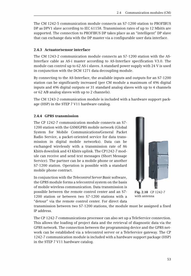
2.4 Communication modules (CM)
53
The CM 1242-5 communication module connects an S7-1200 station to PROFIBUSDP as DPV1 slave according to IEC 61158. Transmission rates of up to 12 Mbit/s aresupported. The connection to PROFIBUS DP takes place as an “intelligent” DP slavethat can exchange data with the DP master via a configurable user data interface.
2.4.3 Actuator/sensor interface
The CM 1243-2 communication module connects an S7-1200 station with the AS-Interface cable as AS-i master according to AS-Interface specification V3.0. Themodule can control up to 62 AS-i slaves. A standard power supply with 24 V is usedin conjunction with the DCM 1271 data decoupling module.
By connecting to the AS-Interface, the available inputs and outputs for an S7-1200station can be significantly increased (per CM module a maximum of 496 digitalinputs and 496 digital outputs or 31 standard analog slaves with up to 4 channelsor 62 A/B analog slaves with up to 2 channels).
The CM 1243-2 communication module is included with a hardware support pack-age (HSP) in the STEP 7 V11 hardware catalog.
2.4.4 GPRS transmission
The CP 1242-7 communication module connects an S7-1200 station with the GSM/GPRS mobile network (GlobalSystem for Mobile Communications/General PacketRadio Service, a packet-oriented service for data trans-mission in digital mobile networks). Data can beexchanged wirelessly with a transmission rate of 86Kbit/s downlink and 43 Kbit/s uplink. The CP1242-7 mod-ule can receive and send text messages (Short MessageService). The partner can be a mobile phone or anotherS7-1200 station. Operation is possible with a standardmobile phone contract.
In conjunction with the Telecontrol Server Basic software,the GPRS module forms a telecontrol system on the basisof mobile wireless communication. Data transmission ispossible between the remote control center and an S7-1200 station or between two S7-1200 stations with a“detour” via the remote control center. For direct datatransmission between two S7-1200 stations, the module must be assigned a fixedIP address.
The CP 1242-7 communications processor can also set up a TeleService connection.This allows the loading of project data and the retrieval of diagnostic data via theGPRS network. The connection between the programming device and the GPRS net-work can be established via a telecontrol server or a TeleService gateway. The CP1242-7 communication module is included with a hardware support package (HSP)in the STEP 7 V11 hardware catalog.
Fig. 2.10 CP 1242-7 with antenna

2 SIMATIC S7-1200 automation system
54
2.5 Further modules
2.5.1 Compact switch module (CSM)
The connection multiplier CSM 1277 unmanaged allowssimple design of an Ethernet network. It includesfour RJ45 sockets with which an S7-1200 station can beconnected to other devices over Industrial Ethernet,for example to other programmable controllers or toHMI stations.
The connection multiplexer is designed for 10/100 MBit/s.It automatically detects the data transfer rate (autosens-ing) and can be used with standard or crossover cables(autocrossover function).
Status LEDs indicate the existing power supply, the portstatus, and the current data traffic. The interface multi-plier does not require configuration.
2.5.2 Power module (PM)
The power supply for the CPU module is either120/230 V AC with 50/60 Hz or 24 V DC. The CPUderives the required internal voltages from thisvoltage.
If the onboard power supply is insufficient, theexternal PM 1207 power supply can be used.The input voltage is 120/230 V AC with a currentconsumption of 1.2/0.7 A. 24 V DC with 2.5 A isavailable at the output.
A status LED on the front indicates that the 24 Voutput voltage is present. The PM 1207 does notrequire configuration.
2.5.3 TS Adapter IE Basic
With TeleService, remote servicing of SIMATICS7 automation systems or HMIdevices is possible using the programming device over a fixed line or wireless net-work. TeleService extends the connection from the programming device via thetelephone network to the programmable controllers. The functions to beperformed, such as programming, are completed using the same tools and func-tionality as if the job was being done locally.
The TS Adapter IE Basic consists of the basic unit and a TS module with the modemor an interface for connecting to an external modem. The basic unit has an Ethernetinterface for connecting to a programming device or programmable controller. Theavailable TS modules are listed in the Table 2.6. The TS-Adapter IE Basic is parame-terized with TeleService in the TIA Portal.
Fig. 2.11 CSM 1277 com-pact switch module
Fig. 2.12 PM 1207 power module
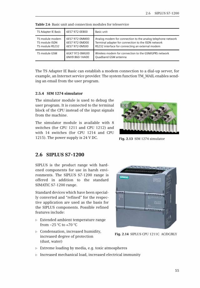
2.6 SIPLUS S7-1200
55
The TS Adapter IE Basic can establish a modem connection to a dial-up server, forexample, an Internet service provider. The system function TM_MAIL enables send-ing an email from the user program.
2.5.4 SIM 1274 simulator
The simulator module is used to debug theuser program. It is connected to the terminalblock of the CPU instead of the input signalsfrom the machine.
The simulator module is available with 8switches (for CPU 1211 and CPU 1212) andwith 14 switches (for CPU 1214 and CPU1215). The power supply is 24 V DC.
2.6 SIPLUS S7-1200
SIPLUS is the product range with hard-ened components for use in harsh envi-ronments. The SIPLUS S7-1200 range isoffered in addition to the standardSIMATIC S7-1200 range.
Standard devices which have been special-ly converted and “refined” for the respec-tive application are used as the basis forthe SIPLUS components. Possible refinedfeatures include:
b Extended ambient temperature range from –25 °C to +70 °C
b Condensation, increased humidity, increased degree of protection (dust, water)
b Extreme loading by media, e.g. toxic atmospheres
b Increased mechanical load, increased electrical immunity
Table 2.6 Basic unit and connection modules for teleservice
TS Adapter IE Basic 6ES7 972-0EB00 Basic unit
TS module modemTS module ISDNTS module RS232
6ES7 972-0MM006ES7 972-0MD006ES7 972-0MS00
Analog modem for connection to the analog telephone networkTerminal adapter for connection to the ISDN networkRS232 interface for connecting an external modem
TS module GSM 6GK7 972-0MG006NH9 860-1AA00
Wireless modem for connection to the GSM/GPRS networkQuadband GSM antenna
Fig. 2.13 SIM 1274 simulator
Fig. 2.14 SIPLUS CPU 1211C AC/DC/RLY
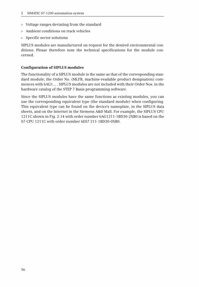
2 SIMATIC S7-1200 automation system
56
b Voltage ranges deviating from the standard
b Ambient conditions on track vehicles
b Specific sector solutions
SIPLUS modules are manufactured on request for the desired environmental con-ditions. Please therefore note the technical specifications for the module con-cerned.
Configuration of SIPLUS modules
The functionality of a SIPLUS module is the same as that of the corresponding stan-dard module; the Order No. (MLFB, machine-readable product designation) com-mences with 6AG1… . SIPLUS modules are not included with their Order Nos. in thehardware catalog of the STEP 7 Basis programming software.
Since the SIPLUS modules have the same functions as existing modules, you canuse the corresponding equivalent type (the standard module) when configuring.This equivalent type can be found on the device's nameplate, in the SIPLUS datasheets, and on the Internet in the Siemens A&D Mall. For example, the SIPLUS CPU1211C shown in Fig. 2.14 with order number 6AG1211-1BD30-2XB0 is based on theS7-CPU 1211C with order number 6ES7 211-1BD30-0XB0.

3.1 Introduction
57
3 Device configuration
3.1 Introduction
Device configuration entails planning the hardware design of your automation sys-tem. Configuration is carried out offline without a connection to the CPU. You canuse this tool to add PLC stations to a project and equip these with modules whichyou then address and parameterize. You also use this tool to carry out the network-ing of PLC stations or the creation of distributed I/O stations.
This chapter primarily describes the configuration of an individual PLC stationwith a CPU 1200 controller and provides an overview of the networking options.Configuration of the distributed I/O is described in Chapters 14.2 “PROFINET IO” onpage 456 and 14.3 “PROFIBUS DP” on page 462.
Start
You can start the device configuration in the Portal view when setting up a newproject if the Open device view checkbox is activated following addition of a CPU.When opening an existing project, start the device configuration by selecting Con-figure a device.
In the Project view, you can start the device configuration in the project tree by dou-ble-clicking on the Devices & networks editor under the project or on the Device con-figuration editor under the PLC station.
The Device view tab shows the occupation of the station rack. You configure the sta-tion in this view. The Network view tab shows the networking between multiple sta-tions. In this view you can add further subnets and stations, and configure theirnetworking (described in Chapter 3.4 “Configuring the network” on page 67). Inthe Topology view tab you configure the geographic arrangement of the Ethernetnetwork.
Working in the Device view
The device configuration shows a rack with the current modules. If several PLCsare present in the project, select the one you wish to edit in the toolbar of theworking window. You can now drag new modules with the mouse from the hard-ware catalog to the rack, or remove existing ones. In the inspector window you canset the properties of the selected module such as the technological functions ofthe CPU or the addresses of the input/output modules.
3 Device configuration
58
Working in the Network view
The Network view shows the stations present in the project and their networking.With the Network button activated, you connect two devices into a network byselecting an interface in a station and dragging it with the mouse to another sta-tion. A subnet is then created automatically. You can connect a station to an existingsubnet by dragging the interface with the mouse to the subnet. With the Connec-tions button activated, you define a connection by selecting a subnet and then thetype of connection from the drop-down list; alternatively, the type of connection isdetermined during programming of the communication functions, for examplewith open user communication.
You set the properties of the selected objects in the inspector window, e.g. the lineconfiguration and the bus parameters, when networking with PROFIBUS.
Working in the Topology view
The Topology view shows the networking between the stations on the Ethernet bussystem. The connections between the device ports are shown. The connections canbe created, changed, or deleted.
In online mode, the Topology view shows the differences between the reference andactual topologies. A topology present online can be adopted offline as configurationinformation.
Save, compile and download
You save the entered data on the hard disk by saving the complete project (usingthe Project > Save command in the main menu). In order to download the configu-ration data to a CPU module, it must first be compiled in a form understandable tothe CPU (using Edit > Compile). Any errors occurring during compilation are indi-cated in the inspector window under Info. Only error-free (consistent) compilationscan be downloaded to the CPU module using Online > Download to device.
Working area of the device configuration
The device configuration shows the project in the Project view. Fig. 3.1 shows theworking area of the device configuration without project tree.
Three views are available in the Working window:
b The Device view shows the current configuration of the PLC station. The config-uration is shown as a graphic in the top part of the window, and as a table in thebottom part.
b In the Network view you can see – if more than one station is present in theproject – the connections between the stations, also as a graphic in the top partof the window and with the existing stations and their interconnections as a tablein the bottom part.

3.1 Introduction
59
You can use the Topology view to display and configure the port connections withan Ethernet network as a graphic in the top part of the window and as a table in thebottom part.
In all cases, you can “fold shut” the bottom part of the working window.
The Inspector window is positioned below the working window. In the Propertiestab, this shows the properties of the object selected in the working window. The Infotab contains general information on the configuration session and the compilation,and the cross-reference list. The Diagnostics tab shows the operating mode of thestations and the message display.
The Hardware catalog is available on the right in the task window. It shows allhardware components which can be configured with the current version of STEP 7.If you select a component in the lowest level of the hardware catalog, a briefdescription of the most important properties is shown in the information area ofthe hardware catalog.
You can change the size of all windows. You can close all windows except the work-ing window, thus providing more space for the working area. The working windowcan also be maximized and displayed as a separate window.
Fig. 3.1 Example of working area of device configuration (Device view)
3 Device configuration
60
Expanding the hardware catalog
If you want to configure a PROFIBUS DP slave that does not appear in the hardwarecatalog, you must install the GSD file provided by the manufacturer. A GSD file(General Station Description file) contains all the PROFIBUS DP slave properties astext with keywords. If you want to configure a PROFINET IO device that does notappear in the hardware catalog, you must install the GSDML file provided by themanufacturer. This is an XML file containing all properties of a PROFINET IO deviceas GSDML (General Station Description Markup Language).
To subsequently install GSD and GSDML files, select the command Options > Installgeneral station description file (GSD) from the main menu. Enter the source path inthe subsequent dialog, and select the file to be installed.
If, after the publication date of STEP 7, new components such as modules come onthe market, these components can be added later to the hardware catalog withhardware support packages (HSP).
To subsequently install support packages, select the command Options > SupportPackages from the main menu. The Detailed information window displays theinstalled products and components as well as operating system information. UnderInstallation of Support Packages, you can select whether you wish to download theupdate from the Internet or add existing support packages from the file system.
3.2 Configuring a station
“Configuring” is understood to be the addition of a station to the project or, with aPLC station, the arranging of the modules in a rack and the fitting of modules withsubmodules.
3.2.1 Adding a PLC station
When creating a new project, you normally add a PLC station at the same time.You can add further PLC and HMI stations in both the Portal view and the Projectview. In the Portal view, you can add a new station in the Devices & networks portalusing the Add new device command. In the Project view, double-click on Add newdevice in the project tree.
Select the desired CPU in the selection window, and assign it a meaningful name.Before clicking on the OK button, make sure that the Open device view check box isactivated in the window at the bottom left.
You have now configured a rack with a CPU module inserted in slot 1. All slots pos-sible for a CPU 1200 are shown on the right of this. The number of slots depends onthe selected CPU. You can open the display to the left of the CPU and thus expandthe rack for inserting communication modules.
3.3 Assigning module parameters
61
3.2.2 Arranging modules
If not already done, start the Device configuration editor in the project tree under-neath the PLC station by double-clicking. To insert a further module, select it in thehardware catalog (the symbol of the module in the lowest catalog level). You arethen provided with a description of the selected module in the information windowof the hardware catalog. The permissible slots in the rack are displayed. Position thenew module by double-clicking on the module symbol or by dragging it with themouse to the subrack. You can position a signal board directly on the CPU modulein the same manner.
You can either delete an inserted module again (remove it from the rack) or replaceit by a different, equivalent one.
3.2.3 Adding an HMI station
Using the Add new device command you can add an HMI station to the project eitherin the Devices & networks portal or in the project tree. Select the desired HMI devicein the selection window, and assign it a meaningful name. Before clicking on the OKbutton, make sure that the Use device wizard check box is activated in the windowat the bottom left if you wish for guidance when starting the configuration. The fur-ther procedure is described in Chapter 4.1.3 “Operand area bit memory” on page82.
3.3 Assigning module parameters
“Parameterization” is understood to be the setting of module properties. These in-clude, for example, setting addresses, enabling interrupts, or defining communica-tion properties.
Module parameterization is carried out for a selected module in the inspector win-dow in the Properties tab. Select the properties group on the left side, and set thevalues in interactive mode on the right. You can stop the setting of properties at anytime and continue later. Only a portion of the total parameters described below canbe assigned to individual modules.
3.3.1 Parameterization of CPU properties
The CPU's operating system operates with the default settings for program execu-tion. You can change these default settings in the hardware configuration duringparameterization of the CPU and match them to your specific requirements. Subse-quent modification is possible at any time.
When starting up, the CPU adopts the settings deviating from the default settingsin STARTUP mode. These settings then apply to further operation.
To parameterize the CPU properties, select the CPU in the working window of thedevice configuration. If the project contains several stations, select the desired sta-tion in the menu bar of the working window.

3 Device configuration
62
You set the name of the PLC station in the General section. Catalog informationabout the CPU is also shown.
In the PROFINET interface section under Ethernet addresses, you set the connec-tion to an Ethernet subnet and define the IP address and the subnet mask. For moreinformation on the format of the IP address, refer to Section “IP address and subnetmask” on page 73. Under Advanced you can parameterize the real-time propertiesof the PROFINET IO communication and the port interconnection (networking ofthe connection).
The parameterization of the digital and analog inputs/outputs is described in3.3.2 “Addressing input and output signals” on page 64.
A high-speed counter (HSC) can count at a frequency of up to 200 kHz when usingan appropriate signal board, and thus much faster than a software counter. Youmust activate the high-speed counter before you can use it. A high-speed counterrequires defined inputs which are then no longer available for other purposes. Fur-ther information on the application and parameterization of high-speed counterscan be found in Chapter 17.1.1 “High-speed counter (HSC)” on page 548.
The pulse generators provide pulses of up to 200 kHz when using an appropriatesignal board. A pulse generator has two modes of operation: PTO (pulse train out-put) and PWM (pulse-width modulation). Pulses are output via a special onboardoutput. Further information on the application and parameterization of pulse gen-erators can be found in Chapter 17.1.2 “Pulse generator” on page 554.
You can set the startup characteristics of the CPU under Startup. This is where youdetermine how the CPU module is to react when the power supply is switched on:
b No startup (CPU remains in STOP mode)
b Warm restart – RUN (the CPU executes the user program)
b Warm restart – operating mode prior to POWER OFF (either STOP or RUN)
The duration for module parameterization for the distributed I/O is monitoredduring a startup. You can set the monitoring time here. A module is considered tobe absent if the monitoring time for it expires. Further information on the CPUstartup can be found in Chapter 5.1.2 “STARTUP mode” on page 118.
In the Cycle section, you set the scan cycle monitoring time with which the process-ing of the main program is monitored. If the cycle monitoring time is exceeded, thisis reported and can lead to the STOP mode. Furthermore, you can activate a fixedminimum cycle time, i.e. the next (cyclic) execution of the main program is onlystarted after this time has elapsed. Further details can be found in Chapter 5.6.3“Cycle time” on page 144.
In the Communication load section you define the time share for communication.In addition to execution of the user program, the CPU also carries out communica-tion tasks, for example data transmission to another PLC station or downloading ofblocks from a programming device. This communication requires time, some ofwhich has to be added to the execution time of the main program. Specification ofthe communication load can be used to control influencing of the cycle time to a

3.3 Assigning module parameters
63
certain extent. The time available for communication is entered as a percentage inthe Communication load parameter. The cycle time is then extended by the factor100 / (100 – communication load).
System and clock memory are operands controlled by the operating system whichcan be queried in the user program. For example, there is a bit memory which indi-cates the occurrence of a diagnostics event, and also a bit memory which changesits signal status at a frequency of 2 Hz. During parameterization of the CPU youactivate the system memories and/or the clock memories and assign addresses tothem. Further information on bit memories in general and on system and clockmemories can be found in Chapter 4.1.3 “Operand area bit memory” on page 82.
In the Web server section you can activate the Web server and set its properties.Further details can be found in Chapter 17.4 “Web server” on page 567.
In the Time of day section you set the time zone for the integral real-time clock andactivate the daylight-saving time setting (difference between daylight-saving andstandard time, start and end of daylight-saving time).
In the Protection section you can protect the program in the CPU from unautho-rized access. Here you select whether access protection is to be switched on, andwhether this is to be just write protection or combined read/write protection. Assigna password if the read or write protection is activated. Anyone in possession of thepassword has unlimited access to the CPU.
The Connection resources section shows the distribution of available connectionsto the programming device and other networked stations.
Fig. 3.2 Example of the address overview of a CPU 1200
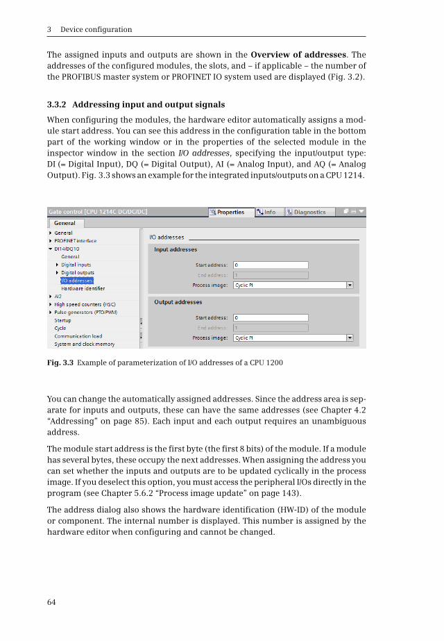
3 Device configuration
64
The assigned inputs and outputs are shown in the Overview of addresses. Theaddresses of the configured modules, the slots, and – if applicable – the number ofthe PROFIBUS master system or PROFINET IO system used are displayed (Fig. 3.2).
3.3.2 Addressing input and output signals
When configuring the modules, the hardware editor automatically assigns a mod-ule start address. You can see this address in the configuration table in the bottompart of the working window or in the properties of the selected module in theinspector window in the section I/O addresses, specifying the input/output type:DI (= Digital Input), DQ (= Digital Output), AI (= Analog Input), and AQ (= AnalogOutput). Fig. 3.3 shows an example for the integrated inputs/outputs on a CPU 1214.
You can change the automatically assigned addresses. Since the address area is sep-arate for inputs and outputs, these can have the same addresses (see Chapter 4.2“Addressing” on page 85). Each input and each output requires an unambiguousaddress.
The module start address is the first byte (the first 8 bits) of the module. If a modulehas several bytes, these occupy the next addresses. When assigning the address youcan set whether the inputs and outputs are to be updated cyclically in the processimage. If you deselect this option, you must access the peripheral I/Os directly in theprogram (see Chapter 5.6.2 “Process image update” on page 143).
The address dialog also shows the hardware identification (HW-ID) of the moduleor component. The internal number is displayed. This number is assigned by thehardware editor when configuring and cannot be changed.
Fig. 3.3 Example of parameterization of I/O addresses of a CPU 1200
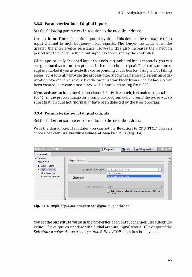
3.3 Assigning module parameters
65
3.3.3 Parameterization of digital inputs
Set the following parameters in addition to the module address:
Use the input filter to set the input delay time. This defines the resistance of aninput channel to high-frequency noise signals. The longer the delay time, thegreater the interference resistance. However, this also increases the detectionperiod until a change in the input signal is recognized by the controller.
With appropriately designed input channels, e.g. onboard input channels, you canassign a hardware interrupt to each change in input signal. The hardware inter-rupt is enabled if you activate the corresponding check box for rising and/or fallingedges. Subsequently provide the process interrupt with a name and assign an orga-nization block to it. You can select the organization block from a list if it has alreadybeen created, or create a new block with a number starting from 200.
If you activate an integrated input channel for Pulse catch, it remains at signal sta-tus “1” in the process image for a complete program cycle, even if the pulse was soshort that it would not “normally” have been detected by the user program.
3.3.4 Parameterization of digital outputs
Set the following parameters in addition to the module address:
With the digital output modules you can set the Reaction to CPU STOP. You canchoose between Use substitute value and Keep last value (Fig. 3.4).
You set the Substitute value in the properties of an output channel. The substitutevalue “0” is output as standard with digital outputs. Signal status “1” is output if theSubstitute a value of 1 on a change from RUN to STOP check box is activated.
Fig. 3.4 Example of parameterization of a digital output channel

3 Device configuration
66
3.3.5 Parameterization of analog inputs
Set the following parameters in addition to the module address:
In Module diagnostics you can activate monitoring of the power supply so that adiagnostics interrupt is generated in the event of a failure.
Use Noise reduction to set the integration time. Because they frequently have alow signal level, analog signals can be “noisy” due to the line frequency. By select-ing an integration time which differs from the line frequency, crosstalk of the linefrequency is reduced (Fig. 3.5).
For the Measurement type you can set Voltage with the ranges ±2.5 V, ±5 V and±10 V or Current (0 to 20 mA). With smoothing in he steps None (1 cycle),Weak (4 cycles), Medium (16 cycles) and Strong (32 cycles) you can prevent excessivevariation of the recorded analog signal.
In Channel diagnostics you can activate the Enable overflow diagnostics andEnable underflow diagnostics check boxes to trigger a diagnostics interrupt whenthe measured value exceeds or falls below the standard range.
3.3.6 Parameterization of analog outputs
Set the following parameters in addition to the module address:
In Module diagnostics you can activate monitoring of the power supply so that adiagnostics interrupt is generated in the event of a failure.
With the analog output modules you can set the Reaction to CPU STOP. You canchoose between Use substitute value and Keep last value.
Fig. 3.5 Example of parameterization of an analog input channel
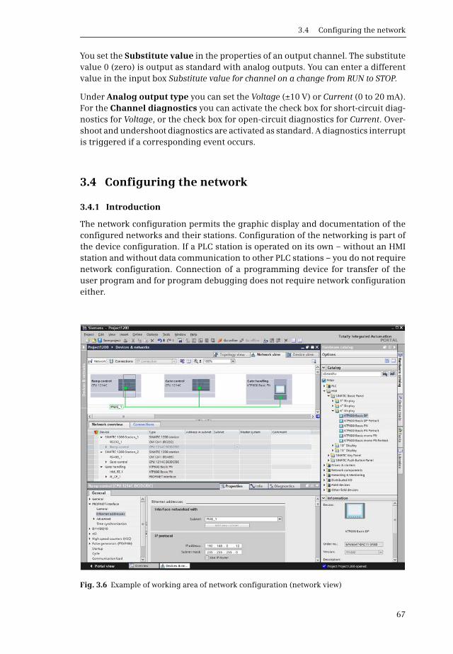
3.4 Configuring the network
67
You set the Substitute value in the properties of an output channel. The substitutevalue 0 (zero) is output as standard with analog outputs. You can enter a differentvalue in the input box Substitute value for channel on a change from RUN to STOP.
Under Analog output type you can set the Voltage (±10 V) or Current (0 to 20 mA).For the Channel diagnostics you can activate the check box for short-circuit diag-nostics for Voltage, or the check box for open-circuit diagnostics for Current. Over-shoot and undershoot diagnostics are activated as standard. A diagnostics interruptis triggered if a corresponding event occurs.
3.4 Configuring the network
3.4.1 Introduction
The network configuration permits the graphic display and documentation of theconfigured networks and their stations. Configuration of the networking is part ofthe device configuration. If a PLC station is operated on its own – without an HMIstation and without data communication to other PLC stations – you do not requirenetwork configuration. Connection of a programming device for transfer of theuser program and for program debugging does not require network configurationeither.
Fig. 3.6 Example of working area of network configuration (network view)
3 Device configuration
68
You can access the network configuration with the project opened in the Portal viewvia Devices & networks and Configure networks or in the Project view with the Devices& networks editor, which is positioned in the project tree underneath the project. Inthe working window of the device configuration, change to the Network view tab(Fig. 3.6).
In the top part of the working window, the Network view graphically displays allPLC, PC, and HMI stations present in the project as well as the networking, providedthis has already been configured during device configuration. The bottom part ofthe working window contains the Network overview, Connections and I/O communi-cation tabs. You can drag further stations with the mouse from the hardware cata-log into the working area and thus add them to the project. The inspector windowshows the properties of the selected object.
3.4.2 Networking stations
“Networking” of stations corresponds to the wiring of modules with communica-tion capability, i.e. a mechanical connection is established. A logical connection isadditionally required in order to transfer data on the cable. The logical connectiondefines the transmission parameters between the modules.
The working window of the hardware editor shows the existing stations with themodules with communication capability. The interfaces for the PROFIBUS,PROFINET, and AS-Interface subnets are highlighted. Communication modulesthat may be present are arranged on the left next to the CPU.
Adding a station in the network configuration
In the hardware catalog under PLC > SIMATIC S7-1200 > CPU > [folder: CPU 12xx…]> [CPU], select the desired CPU and drag it with the mouse into the working area.The graphic shows the CPU as a representative for the complete PLC station withthe existing bus interfaces.
If you drag the CPU to an existing subnet and if the CPU has an interface matchingthe subnet, the interface is directly connected to the subnet when adding.
Adding a communication module in the network configuration
In the hardware catalog under PLC > SIMATIC S7-1200 > Communication modules >[folder: Subnet] > [folder: Modules] > [Module], select the desired communicationmodule and drag it with the mouse into the station graphic on the working area.The module is shown with the existing bus interfaces in the PLC station next to theCPU.
Adding a subnet
Select the desired bus interface in the station graphic and then select the Add sub-net command from the shortcut menu. A subnet corresponding to the bus interfaceis added.
3.4 Configuring the network
69
Networking a station
To network stations, click on the Network button in the toolbar of the working win-dow.
If a subnet has not yet been created, select the bus interface in one of the stationsand drag it to a bus interface of the other station which matches the subnet. Thesubnet is then added; the interfaces are connected by a colored line.
If the matching subnet is already present, select the bus interface in the station anddrag it to the subnet. The interface is connected to the subnet by a colored line.
Properties of the Ethernet network
The network configuration shows the Ethernet connections between several sta-tions as a linear bus connection: all stations are hanging quasi on one line. Actually,an Ethernet connection is a point-to-point connection between the stations: eachstation is connected to exactly one partner station. The PROFINET interface of a CPU1215 has two ports which are connected together by an integrated switch. A linearnetwork can thus quasi be set up.
Modules without this integrated switch must be networked together via an external“distributor” with several connections. You can find these devices in the hardwarecatalog under Network components > IE switches > [Group] > [Device type] > [Device].
In the S7-1200 automation system, a CSM 1277 Ethernet switch is available withfour ports and in S7-1200 design. The switch is not displayed in the network viewsince it does not require any parameters. In the topology view, if all ports areconnected individually, the switch can be found in the hardware catalog under Net-work components > IE switches > Compact switch modules > CSM 1277 unmanaged >[Module].
Disconnecting a module from the subnet or assigning it to a different subnet
If you wish to disconnect a module from the subnet, select the bus interface andthen the Disconnect from subnet command in the shortcut menu. If all moduleshave been disconnected from a subnet, it is shown as an isolated subnet at the topleft in the working area.
If you wish to assign a module to a new subnet, select the bus interface and then theAssign to a new subnet command in the shortcut menu. If several suitable subnetsare available, select the appropriate one from the displayed list.
3.4.3 Node addresses in a subnet
Each module – each “node” – connected to a subnet requires an unambiguousaddress on the subnet (the “node address”) with which the module can beaddressed within the subnet. When assigning node addresses, attention must bepaid to the particular properties of the associated subnet.
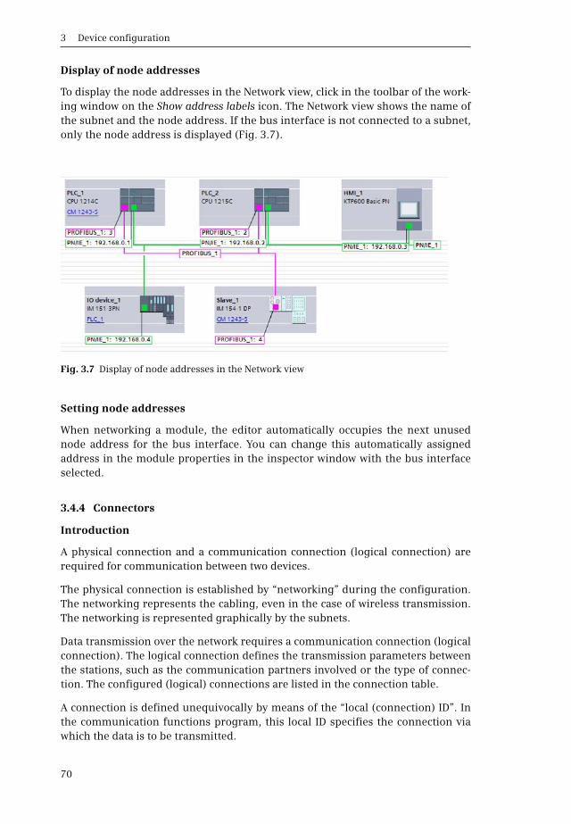
3 Device configuration
70
Display of node addresses
To display the node addresses in the Network view, click in the toolbar of the work-ing window on the Show address labels icon. The Network view shows the name ofthe subnet and the node address. If the bus interface is not connected to a subnet,only the node address is displayed (Fig. 3.7).
Setting node addresses
When networking a module, the editor automatically occupies the next unusednode address for the bus interface. You can change this automatically assignedaddress in the module properties in the inspector window with the bus interfaceselected.
3.4.4 Connectors
Introduction
A physical connection and a communication connection (logical connection) arerequired for communication between two devices.
The physical connection is established by “networking” during the configuration.The networking represents the cabling, even in the case of wireless transmission.The networking is represented graphically by the subnets.
Data transmission over the network requires a communication connection (logicalconnection). The logical connection defines the transmission parameters betweenthe stations, such as the communication partners involved or the type of connec-tion. The configured (logical) connections are listed in the connection table.
A connection is defined unequivocally by means of the “local (connection) ID”. Inthe communication functions program, this local ID specifies the connection viawhich the data is to be transmitted.
Fig. 3.7 Display of node addresses in the Network view
3.4 Configuring the network
71
A connection is either dynamic or static depending on the communication serviceselected. Dynamic connections are not configured whose establishing and clearingdown take place depending on events. Only one non-configured connection to acommunication partner can exist at any time.
Static connections are configured in the connection table; they are establishedduring the startup and are retained throughout the complete program execution.Several connections can be established in parallel to one communication partner.Under “Connection type” in the network configuration you can select the desiredcommunication service.
Connection types
Select the connection type depending on the subnet and the transmission protocol.In most cases this is the S7 connection. You can then exchange data between all S7devices on all subnets. The programming device also uses this connection type forprogramming the PLC and HMI stations.
You use the HMI connection for communication with an HMI station. You use theother connection types, for example, if you wish to transmit data to third-partydevices. This usually takes place by means of a communication module.
Connection resources
Every connection requires connection resources on the communication partnersinvolved for the end point of the connection and for the transition point in a com-munication module. Each CPU has a specific number of possible connections.Restrictions and rules apply to use of the connection resources. For example, notevery connection resource can be used for every connection type.
The operating system of a CPU 1200 simultaneously supports the following asyn-chronous communication connections:
b 1 connection to a programming device
b 3 connections to an HMI device (HMI station)
b 8 connections for Open User Communication
b 3 connections for the S7 communication (PUT/GET) as server
b 8 connections for the S7 communication (PUT/GET) as client
b 1 connection to the Web server (HTTP)
One connection is always reserved for a programming device, and another one foran HMI station (these cannot be used for anything else).
Configuring connections
In order to configure a connection in the network view, click on the Connections but-ton in the toolbar of the working window, and select the connection type in the adja-cent list. The devices suitable for this connection type are then displayed and high-lighted (Fig. 3.8).

3 Device configuration
72
Click with the left mouse button on a station, drag the connection line with themouse button pressed to the other station, and release the button. A connectionwith the connection name is displayed as a blue/white patterned line. Several logi-cal connections can be created on one cable. These connections are then also pres-ent in the connection table in the Connections tab in the bottom part of the workingwindow.
If you wish to determine which connections have been created in a subnet, click theConnections button and move the cursor to the subnet in the graphic display. If youclick on one of the connections listed in the tooltip window, this connection is dis-played highlighted in the Network view.
Connection properties
Under General in the Properties tab, the inspector window shows the connectionpartners, the connection path, and the node addresses. If a station has several suit-able interfaces, you can select the appropriate one from a drop-down list. You canset further connection properties in the bottom part of the Properties window, e.g.which partner is responsible for active establishment of the connection, and thelocal connection ID.
Fig. 3.8 Representation of an HMI connection in the network configuration

3.4 Configuring the network
73
3.4.5 Configuring a PROFINET subnet
To configure a PROFINET subnet, drag the PN interface of one station to the PNinterface of the other station with the mouse. A PROFINET subnet will be createdautomatically. You can also drag a PN interface to an existing PROFINET subnet.
Setting the properties of a PROFINET subnet
To set the properties, select the PROFINET subnet and then the Properties tab in theinspector window. Under General you can assign a different name to the subnet andalso change the subnet ID if appropriate.
Setting the properties of a PN interface
To set the properties, select the PN interface and then the Properties tab in theinspector window. Under General you can set a different name for the interface.Under Ethernet addresses you set the IP address and the subnet mask of the CPU.
Ethernet address (MAC address)
The MAC (Media Access Control) address is an unambiguous address assigned tothe device and defined by the manufacturer. It consists of three bytes with themanufacturer ID and three bytes with the device ID. The MAC address is usuallyprinted on the device and is assigned to the latter during the configuration – ifthis has not already been carried out in the factory. The bytes are assigned in hexa-decimal form (symbols 0 to F); the individual bytes are separated by colons. Exam-ple: 01:23:45:67:89:AB.
IP address and subnet mask
Each station on the Industrial Ethernet subnet which uses the TCP/IP protocolrequires an IP (Internet Protocol) address. SIMATIC S7 supports Version 4 of theInternet protocol (IPv4). The IP address must be unique on the subnet. The IPaddress consists of four bytes, each separated by a dot. Each byte is represented asa decimal number from 0 to 255.
Fig. 3.9 Example of the structure of an IPv4 address
IP address
Subnet address
Subnet mask
Station address
192
192
255
0
168
168
255
0
1
0
0
1
3
0
0
3
The subnet address is left-justified in the IP address and is generated from the bit-by-bit AND operation of the IP address with the subnet mask.
The bit positions of the subnet mask occupied by “1” must be positioned flush left and without gaps.
IP address and subnet mask
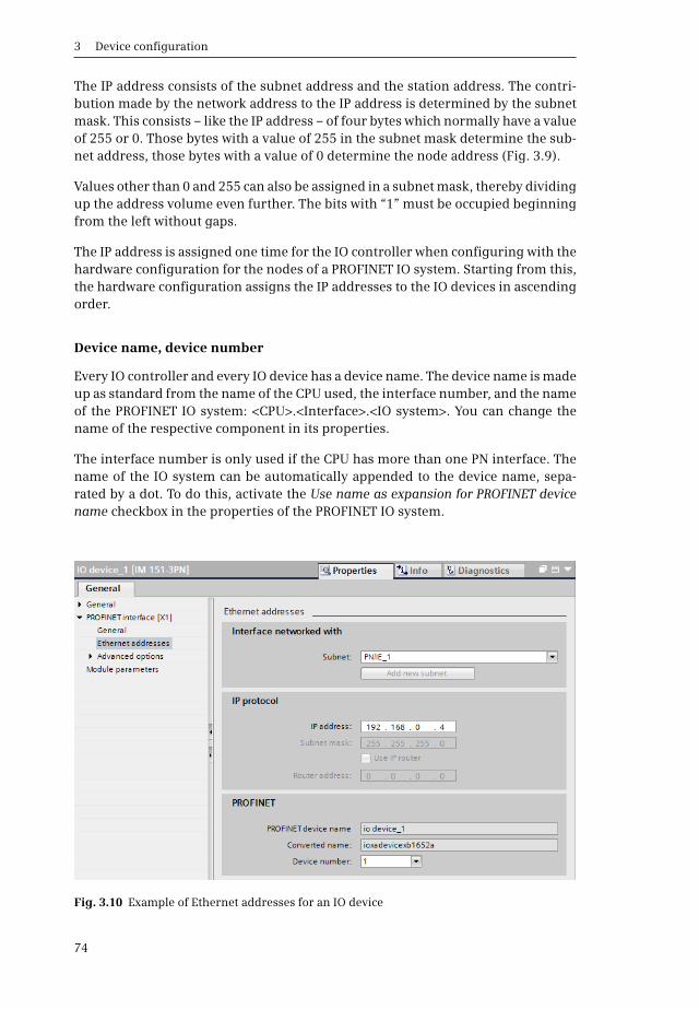
3 Device configuration
74
The IP address consists of the subnet address and the station address. The contri-bution made by the network address to the IP address is determined by the subnetmask. This consists – like the IP address – of four bytes which normally have a valueof 255 or 0. Those bytes with a value of 255 in the subnet mask determine the sub-net address, those bytes with a value of 0 determine the node address (Fig. 3.9).
Values other than 0 and 255 can also be assigned in a subnet mask, thereby dividingup the address volume even further. The bits with “1” must be occupied beginningfrom the left without gaps.
The IP address is assigned one time for the IO controller when configuring with thehardware configuration for the nodes of a PROFINET IO system. Starting from this,the hardware configuration assigns the IP addresses to the IO devices in ascendingorder.
Device name, device number
Every IO controller and every IO device has a device name. The device name is madeup as standard from the name of the CPU used, the interface number, and the nameof the PROFINET IO system: <CPU>.<Interface>.<IO system>. You can change thename of the respective component in its properties.
The interface number is only used if the CPU has more than one PN interface. Thename of the IO system can be automatically appended to the device name, sepa-rated by a dot. To do this, activate the Use name as expansion for PROFINET devicename checkbox in the properties of the PROFINET IO system.
Fig. 3.10 Example of Ethernet addresses for an IO device

3.4 Configuring the network
75
If the names used do not correspond to the conventions of IEC 61158-6-10 (namecomponents basically consisting of lower-case letters, numbers, and hyphens sep-arated by a dot), STEP 7 generates a so-called “converted” name which is then down-loaded to the device (see Fig. 3.10).
As a supplement to the device name, the hardware configuration assigns a devicenumber to each IO device which is independent of the IP address and which youcan change. Using this device number (station number) you can address the IOdevice from the user program, e.g. as a current parameter on a system block.
IP address of the router
A router establishes the connection between two subnets. If the target of a deviceconnection is in a different subnet, the IP address of the corresponding router mustalso be specified. The connections of the router belong to two different subnets, andthe IP addresses must also be selected accordingly.
Setting the interface parameters
If the parameters of the PROFINET interface have not already been set during thehardware configuration, they can be defined during the network configuration.
Prerequisite: a project with two or more stations is open, the device configurationshows the stations in the network view.
b Select the PROFINET interface, e.g. by clicking with the mouse in the graphicdisplay or on the corresponding line in the tabular device or network overview.
b In the Properties tab of the Inspector window, select the Ethernet addressessection under General.
b If the subnet has not yet been created, click on the Add new subnet button to con-nect the interface to a subnet.
b Enter the IP address and the subnet mask.
b Enter whether an IP router is used, and then the router address if applicable.
You can display the addresses of the interfaces using the Show address labels sym-bol in the toolbar of the network view.
3.4.6 Configuring a PROFIBUS subnet
A CPU 1200, together with a CM 1243-5 module as DP master and with a CM 1242-5module as DP slave, can be connected to a PROFIBUS subnet.
To configure a PROFIBUS subnet, drag the DP interface of one stationto the DP inter-face of the other station. A PROFIBUS subnet will be created automatically. You canalso drag a DP interface to an existing PROFIBUS subnet.

3 Device configuration
76
Setting the properties of a PROFIBUS subnet
To set the properties, select the PROFIBUS subnet and then the Properties tab inthe inspector window. Under General you can assign a different name to the sub-net and also change the subnet ID if appropriate. Under Network settings you setthe highest node address, the transmission speed, and the profile in this subnet.You must observe the technical specifications of the involved modules whendoing this (Fig. 3.11).
The selectable bus profiles have the following properties:
b The DP bus profile contains the optimized settings of the bus parameters for de-vices which comply with the requirements of the EN 50170 Volume 2/3, Part 8-2PROFIBUS standard, for example all SIMATIC S7 DP masters and DP slaves.
b Compared to the DP bus profile, the Standard bus profile additionally containsthe option for considering non-configured nodes during calculation of the busparameters, for example nodes from other projects.
b Select the Universal bus profile if the PROFIBUS FMS service is to be used in thePROFIBUS subnet.
b When using the User-defined bus profile, you can set the parameters of thePROFIBUS subnet yourself in the subnet properties. Correct functioning is onlyguaranteed if the bus parameters are matched to one another. You should onlychange the default values if you are familiar with how to configure the bus pro-file for PROFIBUS.
Setting the properties of a DP interface
To set the properties, select the DP interface and then the Properties tab in theinspector window. Under General you can set a different name for the interface.Under PROFIBUS address you set the node address of the CPU.
Every station on the PROFIBUS DP has a node address (station number) with whichit can be addressed unequivocally on the bus. The addresses in a PROFIBUS subnet
Fig. 3.11 Example of network settings on the PROFIBUS

3.4 Configuring the network
77
can be freely assigned in the range from 1 to 126. The node address 0 is reserved asstandard for a programming device, which can be connected temporarily to thePROFIBUS subnet for servicing purposes.
STEP 7 assigns node addresses from 2 upwards as standard in the hardware config-uration. It is recommendable to assign the addresses without gaps.
Under Operating mode – depending on the CM module – the operating mode is pre-set as DP master or DP slave and cannot be changed. The DP slave is an “intelligent”DP slave, for which the user data interface to the DP master must be configuredunder I-slave communication. Further details can be found in the Section 14.3.3“Configuring PROFIBUS DP” on page 467 of Chapter 14.3 “PROFIBUS DP”.
3.4.7 Configuring an AS-i subnet
A CPU 1200, together with the CM 1243-2 module as AS-Interface master, can beconnected to an AS-Interface subnet (Fig. 3.12).
Setting the properties of an AS-i subnet
To set the properties, select the AS-i subnet and then the Properties tab in theinspector window. Under General you can set a different name for the subnet.
Setting the properties of an AS-i master interface
To set the properties, select the AS-i interface in the master and then the Proper-ties tab in the inspector window. Under General, you can give the interfaceanother name and the connection to the AS-Interface subnet is established underAS-Interface.
Fig. 3.12 Example of an AS-i master system with CM 1243-2

3 Device configuration
78
Setting the properties of an AS-i slave interface
To set the properties, select the AS-i interface in the field device and then the Prop-erties tab in the inspector window. Under General you can set a different name forthe interface. Under AS-Interface you set the AS-i subnet used and the nodeaddress. The other settings specify operation on the AS-i subnet (see Chapter 14.4“Actuator/sensor interface” on page 473).

4.1 Operands and tags
79
4 Variables and data types
4.1 Operands and tags
4.1.1 Introduction, overview
In order to control a machine or process, signal states and numerical values areprocessed. Inputs are scanned, and their signal states linked together in accordancewith the control task; the results then control the outputs. It is similar with thenumerical values; these are selected, calculated, compared, and saved. The PLC sta-tion provides the following memory areas for these variable values (Fig. 4.1):
b Peripheral inputs are the memory areas on the input modules. They constitutethe direct interface to the controlled machine, e.g. in order to scan the settingsof control elements or sensors.
b Inputs are an image of the peripheral inputs in the CPU's system memory. Theseare normally processed by the user program when signal states of the machineare to be scanned and linked. The totality of the inputs is the process image input.
b Peripheral outputs are the memory areas on the output modules. They constitutethe direct interface to the controlled machine, e.g. in order to control displays,valves or contactors.
b Outputs are an image of the peripheral outputs in the CPU's system memory.These are normally processed by the user program if the results of the controlfunctions are to be output. The totality of the outputs is the process image out-put.
b Bit memories are a memory area in the CPU's system memory, and are used as aglobal intermediate memory preferably for binary signals.
b Data refers to memory areas in the user memory for binary signals and numeri-cal values. Data is organized in data blocks, which can either be addressed glob-ally from all parts of the user program or which locally manage the data of afunction block. They are then called static local data.
b Temporary local data refers to memory areas assigned by the CPU to a logic blockduring processing. The program can temporarily store signal states and numer-ical values in the block; these lose their validity when processing of the block hasbeen completed.
Access to the signal states and numerical values (the addressing) can be absolute orsymbolic. Absolute addressing uses operands such as %I2.5, for example, whichcomprise the operand ID (I for input in this case) and the memory address (byte 2bit 5 in this case). If a name and a data type are assigned to an operand (symbolic
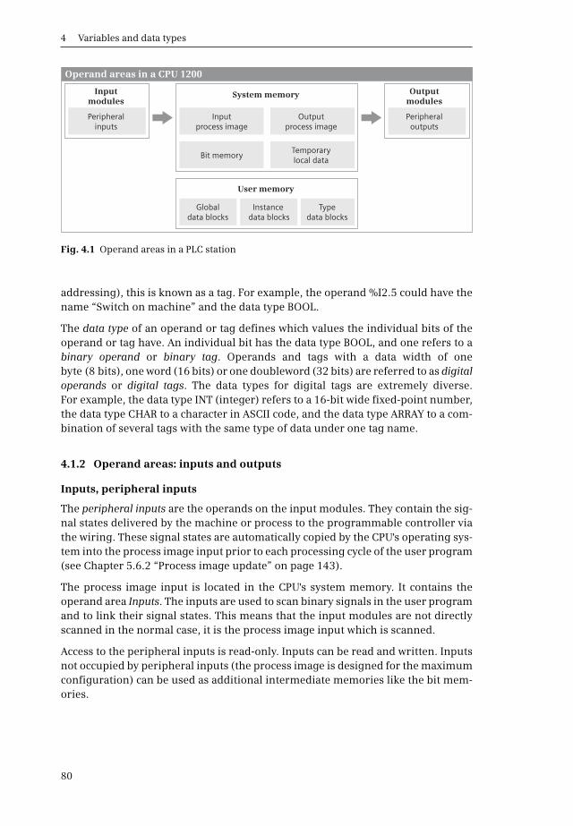
4 Variables and data types
80
addressing), this is known as a tag. For example, the operand %I2.5 could have thename “Switch on machine” and the data type BOOL.
The data type of an operand or tag defines which values the individual bits of theoperand or tag have. An individual bit has the data type BOOL, and one refers to abinary operand or binary tag. Operands and tags with a data width of onebyte (8 bits), one word (16 bits) or one doubleword (32 bits) are referred to as digitaloperands or digital tags. The data types for digital tags are extremely diverse.For example, the data type INT (integer) refers to a 16-bit wide fixed-point number,the data type CHAR to a character in ASCII code, and the data type ARRAY to a com-bination of several tags with the same type of data under one tag name.
4.1.2 Operand areas: inputs and outputs
Inputs, peripheral inputs
The peripheral inputs are the operands on the input modules. They contain the sig-nal states delivered by the machine or process to the programmable controller viathe wiring. These signal states are automatically copied by the CPU's operating sys-tem into the process image input prior to each processing cycle of the user program(see Chapter 5.6.2 “Process image update” on page 143).
The process image input is located in the CPU's system memory. It contains theoperand area Inputs. The inputs are used to scan binary signals in the user programand to link their signal states. This means that the input modules are not directlyscanned in the normal case, it is the process image input which is scanned.
Access to the peripheral inputs is read-only. Inputs can be read and written. Inputsnot occupied by peripheral inputs (the process image is designed for the maximumconfiguration) can be used as additional intermediate memories like the bit mem-ories.
Fig. 4.1 Operand areas in a PLC station
Temporarylocal data
Outputprocess image
Peripheraloutputs
Inputprocess image
Globaldata blocks
Instance data blocks
Typedata blocks
Peripheralinputs
System memory
User memory
Inputmodules
Outputmodules
Bit memory
Operand areas in a CPU 1200
4.1 Operands and tags
81
Outputs, peripheral outputs
The peripheral outputs are the operands on the output modules. They contain thesignal states with which the machine or process is controlled via the wiring. TheCPU's operating system automatically transfers the signal states of the processimage output to the peripheral outputs prior to each processing cycle of the userprogram (see Chapter 5.6.2 “Process image update” on page 143).
The process image output is located in the CPU's system memory. It contains theoperand area Outputs. The outputs are used to save the results of the control func-tions in the user program and to output these to the machine. This means that theoutput modules are not directly written in the normal case, it is the process imageoutput which is written.
Outputs can be read and written. Outputs not occupied by peripheral outputs(the process image is designed for the maximum configuration) can be used as ad-ditional intermediate memories like the bit memories.
Access to the peripheral outputs is write-only. Writing of the peripheral outputs isautomatically tracked by the output process image, and therefore there is no differ-ence in the signal states of the outputs and the peripheral outputs with the sameaddress.
User data area
With SIMATIC S7, every module can have two data areas: A user data area contain-ing input and output data, and a system data area to transfer datasets with diagnos-tic and parameter assignment data.
When the modules are addressed it is irrelevant whether they are located in centralracks or are used as distributed I/O. All modules are arranged equally in the (logi-cal) address volume.
The user data properties of a module depend on the module type. These are digitalor analog I/O signals for signal modules or, for example, control and status infor-mation for communication modules. The amount of user data is module-specific.There are modules which occupy one, two, or more bytes in this area. Occupationalways commences at the relative byte 0. The (logical) address of the relative byte 0is the module start address, which is defined by the hardware configuration.
The user data represent the peripheral operand area, divided into peripheral inputsand peripheral outputs depending on the transfer direction. If the user data is pres-ent in the area of the process images, the CPU automatically takes over dataexchange when updating the process images.
Consistent user data areas
Data consistency means that data is handled together. Transfer of the data blockmust not be interrupted, and the data source and destination must not be changedduring the transfer either. A CPU 1200 receives the data consistency for tags withall elementary data types and system data types. This means a read or write opera-
4 Variables and data types
82
tion for a tag with one of these data types cannot be interrupted.
For example, if in the main program a write operation is presently occurring andan alarm is triggered that interrupts the main program, the CPU finishes the com-plete write operation in the main program before the interrupt routine is started.
For a data block consisting of several tags, the interrupt routine can interrupt thetransmission of the data block after each tag. Simultaneous access from the mainprogram and the interrupt routine can thus destroy the consistency of the data. Thesystem functions DIS_AIRT before and EN_AIRT after the transfer of the data blockin the main program can be used to delay starting the interrupt routine until afterthe data block is transferred. With an ARRAY data field, you can also use the systemfunction UMOVE_BLK.
A CPU 1200 supports a data consistency of 64 bytes for data transfer via PROFINETIO and PROFIBUS DP. If a data field with more than 64 bytes should be transferredconsistently, use the system functions DPRD_DAT and DPWR_DAT.
Note that the “normal” updating of process images can be interrupted followingeach transmitted doubleword.
Diagnostic and parameter data are always transferred consistently in data records,for example diagnostic data with RALRM or parameter data transferred to and frommodules with RDREC and WRREC.
4.1.3 Operand area bit memory
The bit memories are, as it were, the “auxiliary contactors” of the controller.They mainly serve to save binary signal states. They can be treated like outputs, butare not connected “to the outside”. The bit memories are located in the CPU's sys-tem memory; they are thus always available.
The bit memories are used if intermediate results are to be valid beyond blocklimits and are to be processed in several blocks.
Bit memories can be read and written without limitation.
Retentive bit memories
Some of the bit memories can be set “retentive”, i.e. this part retains its signal stateeven when deenergized. Retentivity always starts at memory byte 0 and ends at theset upper limit. You can set the retentivity in the PLC tag table or in the assignmentlist. Further information can be found in the Chapter 5.1.4 “Retentive behavior ofoperands” on page 121.
System memory bits
A CPU 1200 makes a memory byte available whose signal state is controlled by theCPU's operating system. Fig. 4.2 shows the structure of this system memory byte.You define the number of the system memory byte when assigning the CPU param-eters. The tags with default identifiers are entered in the PLC tag table when the sys-
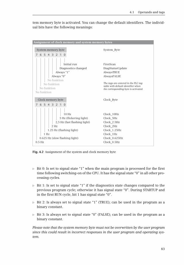
4.1 Operands and tags
83
tem memory byte is activated. You can change the default identifiers. The individ-ual bits have the following meanings:
b Bit 0: Is set to signal state “1” when the main program is processed for the firsttime following switching-on of the CPU. It has the signal state “0” in all other pro-cessing cycles.
b Bit 1: Is set to signal state “1” if the diagnostics state changes compared to theprevious program cycle; otherwise it has signal state “0”. During STARTUP andin the first RUN cycle, bit 1 has signal state “0”.
b Bit 2: Is always set to signal state “1” (TRUE); can be used in the program as abinary constant.
b Bit 3: Is always set to signal state “0” (FALSE); can be used in the program as abinary constant.
Please note that the system memory byte must not be overwritten by the user programsince this could result in incorrect responses in the user program and operating sys-tem.
Fig. 4.2 Assignment of the system and clock memory byte
Clock memory byte Clock_Byte
0.625 Hz (slow flashing light) Clock_0.625Hz0.5 Hz Clock_0.5Hz
1 Hz Clock_1Hz1.25 Hz (flashing light) Clock_1.25Hz
2 Hz Clock_2Hz2,5 Hz (fast flashing light) Clock_2.5Hz
5 Hz (flickering light) Clock_5Hz10 Hz Clock_10Hz
System memory byte System_Byte
No funktionNo funktion
No funktionNo funktion
Always “0” AlwaysFALSEAlways “1” AlwaysTRUE
Diagnostics changed DiagStatusUpdateInitial run FirstScan
7 6 5 4 3 2 1 0
7 6 5 4 3 2 1 0
Assignment of clock memory and system memory bytes
The tags are entered in the PLC tag table with default identifier when the corresponding byte is activated.

4 Variables and data types
84
Clock memory bits
Many processes in the PLC require a periodic signal. These can be implemented us-ing timer functions (clock generator), cyclic interrupts (time-based program execu-tion) or in a particularly simple manner with clock memory bits.
Clock memory bits are memories whose signal state changes periodically with apulse-to-pause ratio of 1:1. The clock memory bits are combined in one byte whoseindividual bits correspond to fixed frequencies (Fig. 4.2). You define the number ofthe clock memory byte when assigning the CPU parameters. The tags with defaultidentifiers are entered in the PLC tag table when the clock memory byte is activated.You can change the default identifiers.
Note that the clock memories are updated asynchronous to processing of the mainprogram. The clock memories are also updated in the startup program.
Please note that the clock memory byte must not be overwritten by the user programsince this could result in incorrect responses in the user program and operating sys-tem.
4.1.4 Operand area data
The operand area Data is organized in data blocks which are present in the usermemory. Data blocks are available in three versions:
b Global data blocks have a data structure which is defined when configuring thedata block.
b Instance data blocks are derived from function blocks. The data structure of aninstance data block is defined in the function block. An instance data block con-tains the values of the block parameters and static local data for calling the func-tion block, for an “instance”. The instance data is local data for the program inthe function block.
b Type data blocks are derived from data types. The data structure of a type datablock is based on a PLC data type or system data type.
Data blocks are global objects which can be addressed in absolute mode using theirnumber, or symbolically using a name. The name of the data block must be uniqueon the CPU. The data tags (data operands) within a data block are local data; theyare declared when creating the data block (global data blocks), the function block(instance data blocks), or the data type (type data blocks). The name of a data tagmust be unique in the data block. In association with the data block, a data tag hasthe characteristic of a global tag.
Data tags can basically be read and written without limitation; limitations may existwith certain (system) data types. The data tags of a data block with the activatedattribute Data block read-only in device cannot be overwritten by the program.
The data present in data blocks can be retentive, i.e. it retains its value even whendeenergized. Further information can be found in the Chapter 5.1.4 “Retentivebehavior of operands” on page 121.
4.2 Addressing
85
4.1.5 Operand area temporary local data
Temporary local data includes operands present in the local data stack (L stack) inthe CPU's system memory. Temporary local data is available in each logic block. Itserves as a buffer for results that are produced during block processing. Its contentsare lost at the end of block processing. The data cannot be accessed by other blocks.
Within the block, the temporary local data can be read and written without limita-tions. Temporary local data cannot be preallocated with a defined value. In order touse temporary local data for meaningful purposes, it must be written before beingread. Temporary local data is addressed symbolically.
The CPUʼs operating system provides 16 KB of temporary local data for block pro-cessing in the startup and in the main program, and 4 KB each for processing of aninterrupt program and the error program. When certain organization blocks arecalled, the operating system transfers start information in the temporary localdata. This start information is displayed in the block interface as input parameters.
The number of temporary local data required by a block can be seen in the callstructure of the user program. With the project open, select the Program blocksfolder in the project tree, and then select the Call structure command from theshortcut menu. The occupied temporary local data is displayed in the call path andper block in the table which is then output.
4.2 Addressing
4.2.1 Signal path
By wiring the machine or plant you define which signals are connected to the PLCstation, and where (Fig. 4.3). An input signal, e.g. the signal from pushbutton+HP01-S10 with the significance “Switch on motor”, is connected to a specific termi-nal on an input module. You configure the slot in which the module is inserted inthe hardware configuration using STEP 7. You use the hardware configuration toset the module start address, from which the addresses of the module channels arederived. This address on the module is simultaneously the address in the processimage. This (logical) address is used to address the signals in the user program.
The CPU automatically copies the signal from the input module into the processimage input every time before cyclic program processing is started, where it isthen addressed as the operand “Input” (e.g. %I5.2). The expression “%I5.2” is theabsolute address.
You can now give this input a name in that you assign a name corresponding to thesignificance of this input signal (e.g. “Switch on motor”) to the absolute address inthe PLC tag table. The expression “Switch on motor” is the symbolic address.
The same applies analogously to the output signals. In the hardware configura-tion you define the slot for the output module and also the module start address.This is then also the address in the process image output. You can also assign aname to this address in the PLC tag table.

4 Variables and data types
86
4.2.2 Absolute addressing of an operand
During absolute addressing, a signal state or a numerical value is addresseddirectly using the address in the operand area. The operand, for example %I2.5,contains the operand ID, the byte address and – with binary operands – the bitaddress separated by a dot. The operand ID contains the operand area and specifi-cation of the operand width (Table 4.1). An absolute address is displayed with a pre-ceding percent sign (%).
Data operands can only be addressed in absolute mode if the Optimized block accessblock attribute is not activated in the data block.
The bits in a byte are counted from right to left, starting with zero. Counting isstarted from the beginning for each byte. Each operand area is organized in bytes.The bytes are counted commencing at the start of the area with zero. With an oper-and of byte width, the number of the byte is specified as the byte address; with anoperand of word width, the number of the least significant byte; and with an oper-and of doubleword width, the least significant byte number in the doubleword.This principle is explained in Fig. 4.4 using the memory bytes MB 24 to MB 27 asexample.
4.2.3 Absolute addressing of an operand area
A block parameter with the VARIANT parameter type can also be supplied with anabsolutely addressed operand area. A pointer is used here containing the operandarea, the start address, the data type, and the number of components (Fig. 4.5).
Fig. 4.3 Signal path from sensor to process image
+HP01-S10
System memory
7 6 5 4 3 2 1 0
Byte 4
Byte 5
Absolute addressing
Process image input
00
77
00
77
Byte 4Relative byte 0
Bit
(Byte 5)Relative byte 1
Peripheral inputs
Input terminals
Input module
Module start address
Slot address
Signal path from the sensor to the process image
The address in the process image is derived from the module start address. In the example, the absolute address of the input signal is: %I5.2.
The slot address identifies a specific module in the station. It contains the numbers of the rack and the number of the slot.
The module start address identifies the module in the “logical” address area of the station. It represents the lowest byte of the module.
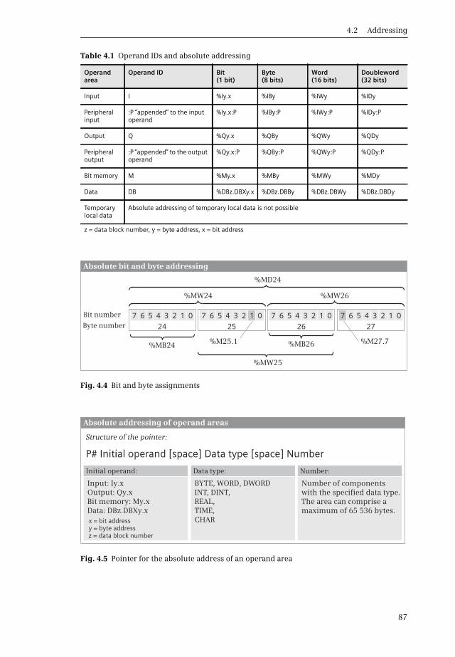
4.2 Addressing
87
Table 4.1 Operand IDs and absolute addressing
Operand area
Operand ID Bit(1 bit)
Byte(8 bits)
Word(16 bits)
Doubleword(32 bits)
Input I %Iy.x %IBy %IWy %IDy
Peripheral input
:P “appended” to the input operand
%Iy.x:P %IBy:P %IWy:P %IDy:P
Output Q %Qy.x %QBy %QWy %QDy
Peripheral output
:P “appended” to the output operand
%Qy.x:P %QBy:P %QWy:P %QDy:P
Bit memory M %My.x %MBy %MWy %MDy
Data DB %DBz.DBXy.x %DBz.DBBy %DBz.DBWy %DBz.DBDy
Temporary local data
Absolute addressing of temporary local data is not possible
z = data block number, y = byte address, x = bit address
Fig. 4.4 Bit and byte assignments
Fig. 4.5 Pointer for the absolute address of an operand area
%MW24
%MD24
%MW26
%MB24
%MW25
%MB26%M25.1 %M27.7
24 25 26 27Byte number
Bit number
Absolute bit and byte addressing
7 6 5 4 3 2 1 0 7 6 5 4 3 2 1 0 7 6 5 4 3 2 1 0 7 6 5 4 3 2 1 0
Input: Iy.xOutput: Qy.xBit memory: My.xData: DBz.DBXy.x
BYTE, WORD, DWORDINT, DINT,REAL,TIME,CHAR
Absolute addressing of operand areas
P# Initial operand [space] data type [space] numberP# Initial operand [space] data type [space] number
Initial operand: Data type: Number:
x = bit addressy = byte addressz = data block number
Structure of the pointer:
Number of components with the specified data type. The area can comprise a maximum of 65 536 bytes.
P# Initial operand [space] Data type [space] Number

4 Variables and data types
88
The start address must be a bit address. The permissible data types are an intersec-tion between the data types of a CPU 1200 and a CPU 300/400, because the pointeris derived from the ANY pointer of a CPU 300/400. The number defines the size ofthe area; it corresponds to the number of components with the specified data type.
Examples: The pointer P#M100.0 DWORD 4 comprises an area of four doublewords,beginning with the memory byte MB 100, and with a size of 16 bytes. The pointerP#DB10.DBX0.0 INT 16 comprises an area of 16 INT tags within data block DB 10,beginning with data byte DB 0, and with a size of 32 bytes.
If a data area is addressed in absolute mode, the Optimized block access block attri-bute must not be activated in the data block. The use of an absolutely addressedoperand area makes sense if there is no tag defined for this area.
4.2.4 Symbolic addressing
During symbolic addressing, an operand is assigned an alphanumeric ID (name,symbol) and a data type. This is called a tag. For example, the operand %I2.5 couldhave the name “Switch on machine” and the data type BOOL. The tag “Switch onmachine” can then be used in the program instead of the operand %I2.5.
Tag names can be made up of letters, digits, and special characters (except doublequotes). No distinction is made between upper and lower case when checking thename.
Symbolic addressing of global tags
Global tags can be addressed by any block in the entire program. They are declaredin the PLC tag table, and have a unique name within the user program. Global tagsare located in the following operand areas: inputs, peripheral inputs, outputs,peripheral outputs, and bit memories.
Global tags must not have a name which has already been assigned to a constant,PLC data type or block. The program editor indicates the name of a global tag inquotation marks.
Symbolic addressing of block-local tags
Block-local tags are declared within a block in the interface definition. They have aunique name within the block. The same tag name can be used in another blockwith another meaning. The operand areas of the block-local tags are
b the temporary local data in the system memory for all logic blocks,
b the block parameters for functions (FC) and function blocks (FB),
b the static local data in the instance data block for function blocks (FB), and
b the data operands for data blocks (DB).
The program editor indicates the name of a block-local tag with a preceding num-ber sign (#). If the name includes special characters, it is additionally indicated inquotation marks.

4.2 Addressing
89
Symbolic addressing of data tags
A data tag is always addressed together with the data block in which it is located.The data tag is thus given the characteristic of a global tag. An example: The tagname “Switch on motor” can be present in both data blocks “Motor 1” and “Motor2”. The address “Motor 1”.“Switch on motor” addresses a different tag than theaddress “Motor 2”.“Switch on motor”. The general symbolic address of a data tag is:“Data block name”.Tag name. All data tags can thus be addressed, even those in aninstance data block.
If the instance data of a function block must be addressed, i.e. the block parametersand static local data, only the tag name, along with a numerical prefix, is specified:#Local data. For a function block, the instance data are local tags. Further details onstatic local data can be found in the Section “Static local data” on page 136.
4.2.5 Addressing a tag part
It is possible to address an area within a tag. This area can be a bit, byte, or word.
With the block attribute IEC check active, the tag must have data type BYTE, WORD,or DWORD; if the IEC check block attribute is deactivated, this can also be a fixed-point data type (USINT, UINT, UDINT, SINT, INT, DINT).
To address a bit in a tag, program tag name. x<bit number>, for a byte, program tagname.b<byte number>, and for a word, program tag name.w<word number>. Thenumbering begins with zero in each case and must remain within the tag length.
Example: A tag with the name Temperature and data type INT is stored in the datablock Store. The highest-value bit (the sign bit of data type INT) is addressed with“Store”.Temperature.x15.
4.2.6 Addressing constants
A constant is a fixed numerical value. The notation for a directly entered constantand the value range depend on the required data type (see Table 4.4 on page 96).Constants in floating-point format can be entered in exponential format (e.g.+1.234567E+02) or in decimal format (e.g. -123.4567).
Globally valid constants can be assigned a name in the PLC tag table in the User con-stants tab. Letters, digits, and special characters – except double quotes – are per-missible for the name. All elementary data types are permissible.
The name of a constant is unique on the CPU. A name with which a PLC tag, PLC datatype, or block has already been identified cannot be assigned to a constant. No dis-tinction is made between upper and lower case when checking the name. The pro-gram editor represents a symbolically addressed constant in quotation marks.
4.2.7 Indirect addressing
Indirect addressing allows you to address operands whose address is only deter-mined during runtime. You can thus, for example, let program parts be processedseveral times in a loop and use a different operand each time.

4 Variables and data types
90
Since with indirect addressing the addresses are only calculated during runtime,the danger exists that memory areas can be overwritten unintentionally. The auto-mation system could then react in an unexpected manner! Therefore be extremelycareful when using indirect addressing!
Indirect addressing of field components
The index of a field component can be a tag whose value is only specified at runtimeand which can be changed. Fixed-point data types are permitted as data type of theindex tags (SINT, INT, DINT, USINT, UINT, and UDINT). The value of the index tagsmay range only within the defined limits of the field tags.
Example: If MeasuredValues is the name of an ARRAY tag and Index is the name ofan INT tag, a field component can be addressed with #MeasuredValues[#Index].
Examples of the indirect addressing of a data field can be found in the Chapters7.6.1 “Jump functions in the ladder logic” on page 242, 8.6.1 “Jump functions in thefunction block diagram” on page 280, and 9.6.3 “Control statements” in Section“FOR statement” on page 311.
Indirect addressing with PEEK and POKE (SCL)
PEEK and POKE address a value in an operand area whose address (memory loca-tion) can be set during runtime. PEEK reads the value of an operand, POKE writes avalue to an operand. POKE_BLK transfers an indirectly addressed operand area(Fig. 4.6).
The operand areas addressed with PEEK and POKE are inputs, outputs, memorybits, and data blocks. The parameter AREA with the data type BYTE defines the oper-and area together with the parameter DBNUMBER (Table 4.2). The byte address is atthe parameter BYTEOFFSET. For a binary operand, the bit number is added at theparameter BITOFFSET. DBNUMBER, BYTEOFFSET, and BITOFFSET have data typeDINT. In the framework of the implicit data type conversion, these parameters canalso be supplied with tags that have other fixed-point data types.
PEEK reads the value of a digital operand and makes it available as a function value.The preallocated data type is BYTE; it is used to read one byte. If two bytes shouldbe read, note the instruction PEEK_WORD; for four bytes, PEEK_DWORD.
PEEK_BOOL reads the value of a binary operand and makes it available as a functionvalue.
POKE writes the value specified at the parameter VALUE with data type BYTE,WORD, or DWORD (corresponding to one, two, or four bytes) to the specified oper-and area.
POKE_BOOL writes the value (data type BOOL) specified at the parameter VALUE tothe specified binary operand.
POKE_BLK transfers a source operand area, defined with the parameters AREA_SRC,DBNUMBER_SRC, and BYTEOFFSET_SRC, to a operand area defined with the param-
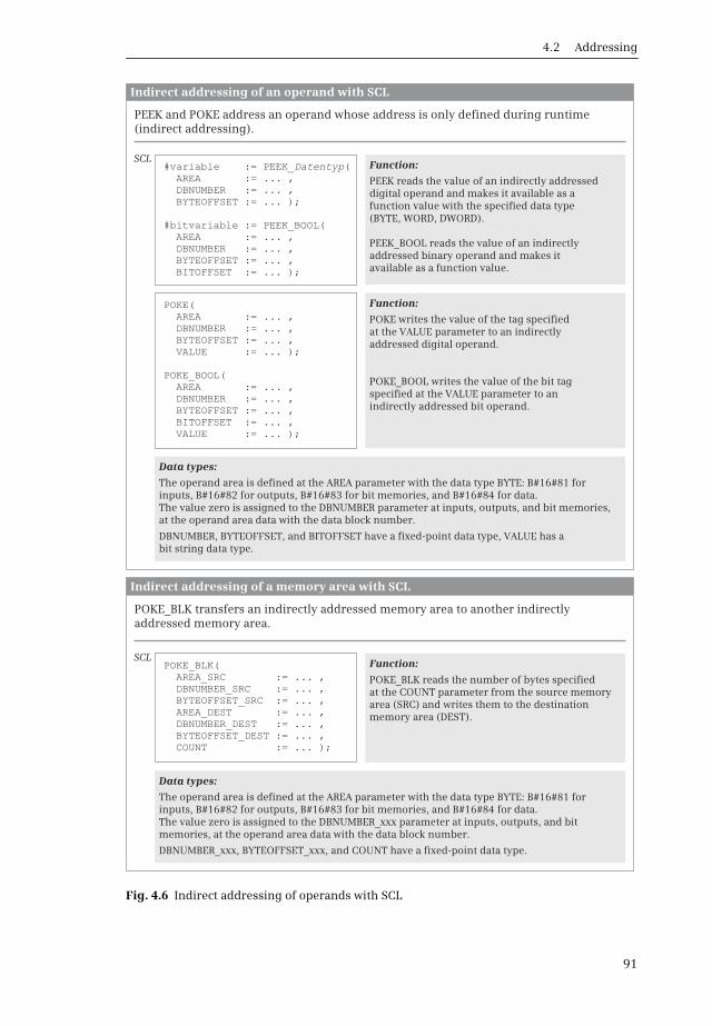
4.2 Addressing
91
Fig. 4.6 Indirect addressing of operands with SCL
Indirect addressing of an operand with SCL
Indirect addressing of a memory area with SCL
SCL
SCL
Function:
Function:
Function:
Data types:
The operand area is defined at the AREA parameter with the data type BYTE: B#16#81 for inputs, B#16#82 for outputs, B#16#83 for bit memories, and B#16#84 for data.
Data types:
The operand area is defined at the AREA parameter with the data type BYTE: B#16#81 for inputs, B#16#82 for outputs, B#16#83 for bit memories, and B#16#84 for data.
#variable := PEEK (AREA := ,
_Datentyp...
DBNUMBER := ... ,BYTEOFFSET := ... );
#bitvariable := PEEK_BOOL(AREA := ,DBNUMBER := ... ,BYTEOFFSET := ... ,BITOFFSET := ... );
...
POKE_BLK(AREA_SRC := ,...DBNUMBER_SRC := ... ,BYTEOFFSET_SRC := ... ,AREA_DEST := ,DBNUMBER_DEST := ... ,BYTEOFFSET_DEST := ... ,COUNT := ... );
...
POKE(AREA := ,...DBNUMBER := ... ,BYTEOFFSET := ... ,VALUE := ... );
POKE_BOOL(AREA := ,DBNUMBER := ... ,BYTEOFFSET := ... ,BITOFFSET := ... ,VALUE := ... );
...
PEEK and POKE address an operand whose address is only defined during runtime (indirect addressing).
PEEK reads the value of an indirectly addressed digital operand and makes it available as a function value with the specified data type (BYTE, WORD, DWORD).
PEEK_BOOL reads the value of an indirectly addressed binary operand and makes it available as a function value.
POKE writes the value of the tag specified at the VALUE parameter to an indirectly addressed digital operand.
POKE_BOOL writes the value of the bit tag specified at the VALUE parameter to an indirectly addressed bit operand.
The value zero is assigned to the DBNUMBER parameter at inputs, outputs, and bit memories, at the operand area data with the data block number.
DBNUMBER, BYTEOFFSET, and BITOFFSET have a fixed-point data type, VALUE has a bit string data type.
POKE_BLK transfers an indirectly addressed memory area to another indirectly addressed memory area.
POKE_BLK reads the number of bytes specified at the COUNT parameter from the source memory area (SRC) and writes them to the destination memory area (DEST).
The value zero is assigned to the DBNUMBER_xxx parameter at inputs, outputs, and bit memories, at the operand area data with the data block number.
DBNUMBER_xxx, BYTEOFFSET_xxx, and COUNT have a fixed-point data type.

4 Variables and data types
92
eters AREA_DEST, DBNUMBER_DEST, and BYTEOFFSET_DEST. The number of bytestransferred is specified in the COUNT parameter.
Example: The values in a bit memory address area should be deleted. The memoryrange begins at the address #M_adr and is #M_anz bytes long. Both tags aredeclared with the INT data type.
FOR #i := #M_adr TO #M_adr + #M_anz - 1 DO POKE(area := 16#83, dbnumber := 0, byteOffset := #i, value := 16#00);END_FOR;
The tag #i with data type INT is used as a loop-control tag in the FOR statement andcontains the address of the memory byte that will now be overwritten with 16#00.
4.3 General information on data types
4.3.1 Overview of data types
Data types define the properties of tags, basically the representation of the contentsand the permissible ranges. STEP 7 provides predefined data types. The data typesare globally available and can be used in any block. A distinction is made between:
b Elementary data types which are predefined and can have a width of up to onelong word (64 bits)
b Structured data types, comprising a combination of elementary data types
b Parameter types for transfer of block parameters to functions and function blocks
b PLC data types whose structure is defined by the user,
b System data types with a fixed structure and defined in STEP 7, and
b Hardware data types defined by the hardware configuration
When linking tags, e.g. when comparing or adding, or when supplying blockparameters, the tags involved must have the same or a comparable data type. Theblock attribute IEC check governs the test for a comparable data type: If it is acti-vated, the test is stricter. The block attribute Optimized block access can also play a
Table 4.2 Assignment of the AREA and DBNUMBER parameters
Operand area Assignment of the AREA parameter
Assignment of the DBNUMBER parameter
Inputs B#16#81 0
Outputs B#16#82 0
Bit memory B#16#83 0
Data B#16#84 Data block number
4.3 General information on data types
93
role in the application of data types. Further details can be found in the section“Attributes” on page 129 of Chapter 5.3.2 “Editing block properties”.
The data types of tags can be converted. This may happen automatically with theimplicit data type conversion or with functions for (explicit) data type conversion(see Chapter 11.6 “Conversion functions (Conversion of data type)” on page 376).
4.3.2 Implicit data type conversion
The implicit data type conversion occurs automatically when a function is executedif the data types of the involved tags are compatible. It always applies duringimplicit data type conversion that the bit length of the source data type must notexceed that of the destination data type. For example, a tag with data formatDWORD (source data type) cannot be applied to a block parameter which expectsdata type WORD (destination data type). The programmed bit length must agreewith the expected bit length for an in-out parameter. The scope of implicit data typeconversion depends on the block attribute IEC check (see Table 4.3).
For LAD and FBD, the implicit conversion from a smaller data width to a larger datawidth is indicated with a gray symbol at the function inputs and outputs. Toimprove clarity, implicit data type conversion can also be programmed with SCL.The statement is Source data type_TO_Destination data type, for example
#var_word := BYTE_TO_WORD(#var_byte);
Where an implicit conversion is possible, the bit pattern of the source tags is trans-ferred unchanged and right-justified to the target tag. Any free bit positions are filledwith zeros. For a possible implicit conversion to a floating-point data type, the formatis transformed (from “–1” to “–1.0”).
4.3.3 Overlaying tags (data type views)
A tag can be “overlaid” by a further data type. It is then possible to address the con-tents of tags completely or partially using various data types.
You overlay a tag with a further data type using the keyword AT. You can overlayseveral data type definitions over a tag which are differentiated by different names.A default setting with fixed values (initialization) is not possible.
Example: You declare an input parameter in the block interface with Station as thename and STRING[12] as the data type. You can overlay this input parameter withan additional STRUCT data type with the name Length and the components maximaland actual, each with the data type USINT (Fig. 4.7). You can now address the cur-rent length of the tags #Station with #Length.actual in the block program.
You can only program the overlaying with further data types in the interface of logicblocks. In addition, the block attribute Optimized block access must be deactivated.The memory requirements of the overlaying data type definition must not begreater than the “original” tag (the new data type must “fit” into the tag).
You use a overlaying data type definition like any other tag, but only locally in theblock. In the example, the calling block writes a string into the input parameter

4 Variables and data types
94
Table 4.3 Implicit data type conversion
to
from BO
OL
BY
TE
WO
RD
DW
OR
D
USI
NT
UIN
T
UD
INT
SIN
T
INT
DIN
T
REA
L
LREA
L
TIM
E
TOD
DA
TE
DTL
CH
AR
STR
ING
BOOL
BYTE x x O O O KF O O O
WORD x O O KF O O
DWORD O KF O O
USINT O O O x x x x x x
UINT O O x x x x O
UDINT O x O
SINT KF x x x x
INT S KF x x x
DINT S S KF x O
REAL x
LREAL
TIME O O
TOD O O
DATE O O
DTL
CHAR O x
STRING
Implicit data type conversion is possible: X Independent of attribute IEC checkO With deactivated attribute IEC checkKF only with LAD and FBD with deactivated attribute IEC checkS only with SCL with deactivated attribute IEC check
Fig. 4.7 Example of declaration of a “overlaid” data type
4.4 Elementary data types
95
#Station; the superimposing data type definition as a USINT structure is not acces-sible to it.
No overlaying with data types is possible for an organization block, because theOptimized block access attribute is always active.
Only the tags in the temporary local data can be overlaid with additional data typesin an FC block.
In a function block, the tags with additional data types can be overlaid in all decla-ration subsections of the block interface. If the in-out parameter has an elementarydata type, overlaying is only possible with an elementary data type. If the in-outparameter has a structured data type, overlaying is only possible with a structureddata type.
4.4 Elementary data types
Elementary data types have a width of 1, 8, 16, 32, or 64 bits (Table 4.4). The datatypes BCD16 and BCD 32 are not data types in the closer sense – they cannot beassigned to a tag; they are only relevant to data type conversion.
4.4.1 Bit-serial data types BOOL, BYTE, WORD and DWORD
A tag with data type BOOL represents a bit value (e.g. input %I1.0). The tag can havethe value “0” or “1”, or FALSE or TRUE (Fig. 4.8).
A tag with data type BYTE occupies 8 bits. The individual bits have no significance.The notation for constants is 16#00 to 16#FF.
A tag with data type WORD occupies 16 bits. The individual bits have no positionalsignificance. The notation for constants is 16#0000 to 16#FFFF. A constant of wordwidth can also be written as a 16-bit binary number (2#0000_…_0000 to2#1111_…_1111) or as a 28-bit unsigned decimal number B#(0,0) to B#(255,255).
A tag with data type DWORD occupies 32 bits. The individual bits have no positionalsignificance. The notation for constants is 16#0000_0000 to 16#FFFF_FFFF. A con-stant of doubleword width can also be written as a 32-bit binary number(2#0000_..._0000 to 2#1111_..._1111) or as a 48-bit unsigned decimal numberB#(0,0,0,0) to B#(255,255,255,255).
4.4.2 BCD-coded numbers BCD16 and BCD32
BCD-coded numbers do not have their own data type. For a BCD number, use thedata type WORD or DWORD and enter only the numbers 0 to 9 or 0 and F for the signin hexadecimal form (16#xxxx or 16#xxxx_xxxx) (Fig. 4.9).
BCD-code numbers are used, for example, in association with the conversion func-tions. The sign of a BCD-coded number is located in the left-justified (highest) de-cade. Thus one decade is lost for the number range.
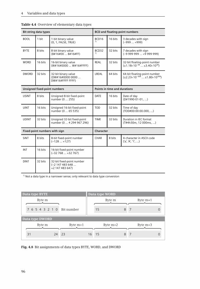
4 Variables and data types
96
Table 4.4 Overview of elementary data types
Bit string data types BCD and floating-point numbers
BOOL 1 bit 1-bit binary value(0, 1, FALSE, TRUE)
BCD16 1)
16 bits 3 decades with sign (–999 … +999)
BYTE 8 bits 8-bit binary value(B#16#00 … B#16#FF)
BCD32 1)
32 bits 7 decades with sign (–9 999 999 … +9 999 999)
WORD 16 bits 16-bit binary value(W#16#0000 … W#16#FFFF)
REAL 32 bits 32-bit floating-point number (±1.1810–38 … ±3.401038)
DWORD 32 bits 32-bit binary value(DW#16#0000 0000 …DW#16#FFFF FFFF)
LREAL 64 bits 64-bit floating-point number (±2.2310–308 … ±1.8010308)
Unsigned fixed-point numbers Points in time and durations
USINT 8 bits Unsigned 8-bit fixed-point number (0 … 255)
DATE 16 bits Date of day(D#1990-01-01, …)
UINT 16 bits Unsigned 16-bit fixed-point number (0 … 65 535)
TOD 32 bits Time of day(TOD#00:00:00.000, …)
UDINT 32 bits Unsigned 32-bit fixed-point number (0 … 4 294 967 296)
TIME 32 bits Duration in IEC format(T#4h30m, 12 000ms, …)
Fixed-point numbers with sign Character
SINT 8 bits 8-bit fixed-point number (–128 … +127)
CHAR 8 bits A character in ASCII code(’a’, ’A’, ’1’, …)
INT 16 bits 16-bit fixed-point number (–32 768 … +32 767)
DINT 32 bits 32-bit fixed-point number (–2 147 483 648 …+2 147 483 647)
1) Not a data type in a narrower sense; only relevant to data type conversion
Fig. 4.8 Bit assignments of data types BYTE, WORD, and DWORD
7 6 5 4 3 2 1 0 7
723
15
1531
0
016
8
824
Byte m
Byte mByte m
Bit number
Byte m+1
Byte m+1
Byte m+2 Byte m+3
Data type DWORD
Data type WORDData type BYTE
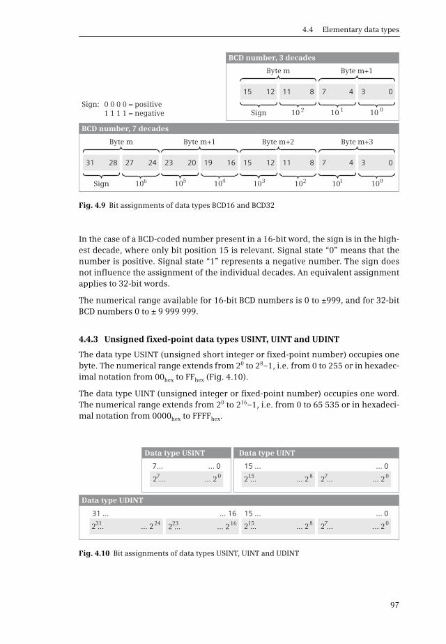
4.4 Elementary data types
97
In the case of a BCD-coded number present in a 16-bit word, the sign is in the high-est decade, where only bit position 15 is relevant. Signal state “0” means that thenumber is positive. Signal state “1” represents a negative number. The sign doesnot influence the assignment of the individual decades. An equivalent assignmentapplies to 32-bit words.
The numerical range available for 16-bit BCD numbers is 0 to ±999, and for 32-bitBCD numbers 0 to ± 9 999 999.
4.4.3 Unsigned fixed-point data types USINT, UINT and UDINT
The data type USINT (unsigned short integer or fixed-point number) occupies onebyte. The numerical range extends from 20 to 28–1, i.e. from 0 to 255 or in hexadec-imal notation from 00hex to FFhex (Fig. 4.10).
The data type UINT (unsigned integer or fixed-point number) occupies one word.The numerical range extends from 20 to 216–1, i.e. from 0 to 65 535 or in hexadeci-mal notation from 0000hex to FFFFhex.
Fig. 4.9 Bit assignments of data types BCD16 and BCD32
Fig. 4.10 Bit assignments of data types USINT, UINT and UDINT
Byte m
Byte m
Byte m+1
Byte m+1
Byte m+2 Byte m+3
10Sign
Sign: 0 0 0 0 = positive1 1 1 1 = negative Sign
10
10
10
10
10
10
10 10 10 01234
0
5
1
6
2
7
7
15
15
2331 3
3
11
11
1927 4
4
12
12
2028 0
0
8
8
1624
BCD number, 3 decades
BCD number, 7 decades
31 ... 15 ...
15 ...7...
... 16 ... 0
... 0... 0
Data type UDINT
Data type UINTData type USINT
2 ...
2 ...2 ...
... 2
... 2... 2
7
77
0
00
2 ...
2 ...
... 2
... 2
15
15
8
8
2 ... ... 223 162 ... ... 231 24
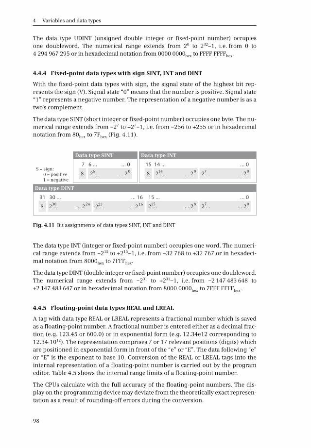
4 Variables and data types
98
The data type UDINT (unsigned double integer or fixed-point number) occupiesone doubleword. The numerical range extends from 20 to 232–1, i.e. from 0 to4 294 967 295 or in hexadecimal notation from 0000 0000hex to FFFF FFFFhex.
4.4.4 Fixed-point data types with sign SINT, INT and DINT
With the fixed-point data types with sign, the signal state of the highest bit rep-resents the sign (V). Signal state “0” means that the number is positive. Signal state“1” represents a negative number. The representation of a negative number is as atwo's complement.
The data type SINT (short integer or fixed-point number) occupies one byte. The nu-merical range extends from –27 to +27–1, i.e. from –256 to +255 or in hexadecimalnotation from 80hex to 7Fhex (Fig. 4.11).
The data type INT (integer or fixed-point number) occupies one word. The numeri-cal range extends from –215 to +215–1, i.e. from –32 768 to +32 767 or in hexadeci-mal notation from 8000hex to 7FFFhex.
The data type DINT (double integer or fixed-point number) occupies one doubleword.The numerical range extends from –231 to +231–1, i.e. from –2 147 483 648 to+2 147 483 647 or in hexadecimal notation from 8000 0000hex to 7FFF FFFFhex.
4.4.5 Floating-point data types REAL and LREAL
A tag with data type REAL or LREAL represents a fractional number which is savedas a floating-point number. A fractional number is entered either as a decimal frac-tion (e.g. 123.45 or 600.0) or in exponential form (e.g. 12.34e12 corresponding to12.34·1012). The representation comprises 7 or 17 relevant positions (digits) whichare positioned in exponential form in front of the “e” or “E”. The data following “e”or “E” is the exponent to base 10. Conversion of the REAL or LREAL tags into theinternal representation of a floating-point number is carried out by the programeditor. Table 4.5 shows the internal range limits of a floating-point number.
The CPUs calculate with the full accuracy of the floating-point numbers. The dis-play on the programming device may deviate from the theoretically exact represen-tation as a result of rounding-off errors during the conversion.
Fig. 4.11 Bit assignments of data types SINT, INT and DINT
31 30 ... 15 ...
15 14 ...7 6 ...
... 16 ... 0
... 0... 0
Data type DINT
Data type INTData type SINT
2 ...
2 ...2 ...S S
S ... 2
... 2... 2
7
76
0
00
2 ...
2 ...
... 2
... 2
15
14
8
8
2 ... ... 223 162 ... ... 230 24
S = sign:0 = positive1 = negative

4.4 Elementary data types
99
Data type REAL
The valid range of values of a REAL tag (normalized 32-bit floating-point number)is between the limits:
–3,402 823 10+38 to –1.175 494 10–38
±0+1.175 494 10–38 to +3.402 823 10+38
A tag with data type REAL consists internally of three components: the sign, the8-bit exponent to base 2, and the 23-bit mantissa. The sign can have the values “0”(positive) or “1” (negative). The exponent is saved increased by a constant (bias,+127) so that it has a range of values from 0 to 255. The mantissa represents thefractional part. The whole number part of the mantissa is not stored, because it isalways equal to 1 within the valid range of values (Fig. 4.12).
Table 4.5 Internal range limits of a floating-point number
Sign Exponent with REAL
Exponent with LREAL
Mantissa Meaning
0 255 2047 Not equal to 0 Not a valid floating-point number (+NaN, Not a Number)
0 255 2047 0 +Inf, Infinity
0 1 … 254 1 … 2046 Any Positive, normalized floating-point number
0 0 0 Not equal to 0 Positive, denormalized floating-point number
0 0 0 0 + Zero
1 0 0 0 – Zero
1 0 0 Not equal to 0 Negative, denormalized floating-point number
1 1 … 254 1 … 2046 Any Negative, normalized floating-point number
1 255 2047 0 – Inf, Infinity
1 255 2047 Not equal to 0 Not a valid floating-point number (–NaN, Not a Number)
Fig. 4.12 Bit assignments of data types REAL and LREAL
31 30 ...
63 62 ...
S = sign of mantissa
... 23
... 52
Data type REAL
Data type LREAL
Exponent
Exponent
Mantissa
Mantissa
2 ...
2 ...
S
S
... 2
... 2
7
10
0
0
22 ...
51 ...
... 0
... 0
2 ...
2 ...
2
2
... 2
... 2
–2
–2
–1
–1
–23
–52
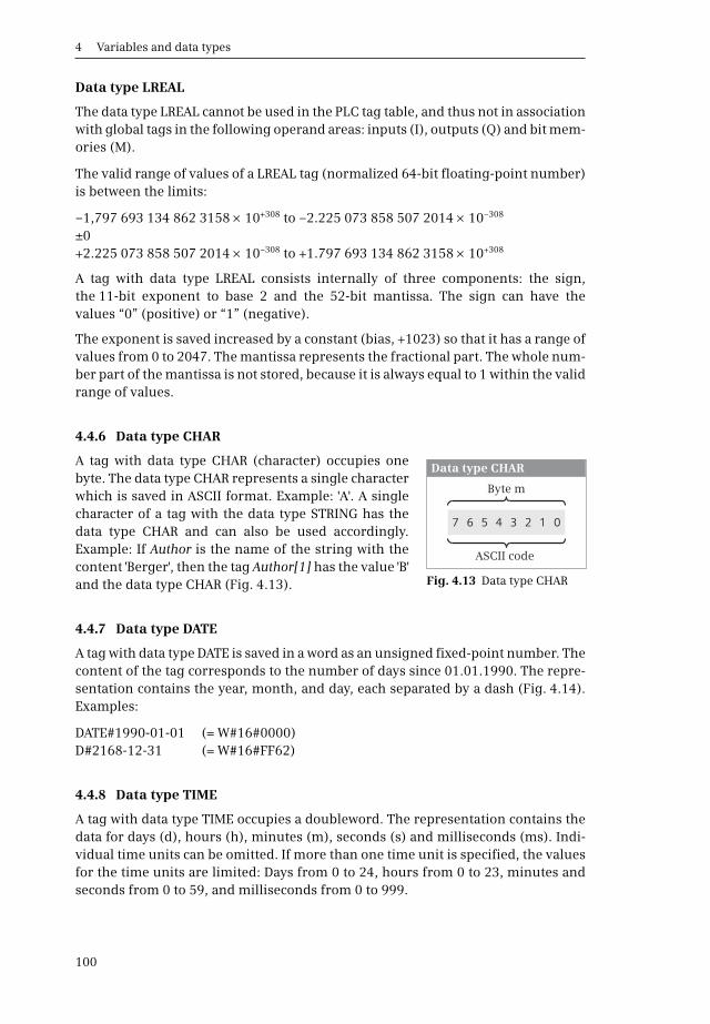
4 Variables and data types
100
Data type LREAL
The data type LREAL cannot be used in the PLC tag table, and thus not in associationwith global tags in the following operand areas: inputs (I), outputs (Q) and bit mem-ories (M).
The valid range of values of a LREAL tag (normalized 64-bit floating-point number)is between the limits:
–1,797 693 134 862 3158 10+308 to –2.225 073 858 507 2014 10–308
±0+2.225 073 858 507 2014 10–308 to +1.797 693 134 862 3158 10+308
A tag with data type LREAL consists internally of three components: the sign,the 11-bit exponent to base 2 and the 52-bit mantissa. The sign can have thevalues “0” (positive) or “1” (negative).
The exponent is saved increased by a constant (bias, +1023) so that it has a range ofvalues from 0 to 2047. The mantissa represents the fractional part. The whole num-ber part of the mantissa is not stored, because it is always equal to 1 within the validrange of values.
4.4.6 Data type CHAR
A tag with data type CHAR (character) occupies onebyte. The data type CHAR represents a single characterwhich is saved in ASCII format. Example: 'A'. A singlecharacter of a tag with the data type STRING has thedata type CHAR and can also be used accordingly.Example: If Author is the name of the string with thecontent 'Berger', then the tag Author[1] has the value 'B'and the data type CHAR (Fig. 4.13).
4.4.7 Data type DATE
A tag with data type DATE is saved in a word as an unsigned fixed-point number. Thecontent of the tag corresponds to the number of days since 01.01.1990. The repre-sentation contains the year, month, and day, each separated by a dash (Fig. 4.14).Examples:
DATE#1990-01-01 (= W#16#0000)D#2168-12-31 (= W#16#FF62)
4.4.8 Data type TIME
A tag with data type TIME occupies a doubleword. The representation contains thedata for days (d), hours (h), minutes (m), seconds (s) and milliseconds (ms). Indi-vidual time units can be omitted. If more than one time unit is specified, the valuesfor the time units are limited: Days from 0 to 24, hours from 0 to 23, minutes andseconds from 0 to 59, and milliseconds from 0 to 999.
Fig. 4.13 Data type CHAR
7 6 5 4 3 2 1 0
Byte m
ASCII code
Data type CHAR

4.5 Structured data types
101
The content of the tag is interpreted as milliseconds (ms) and saved as a 32-bitfixed-point number with sign. The range of values extends from TIME#–24d20h31m23s648ms (T#–24d20h31m23s648ms) to TIME#24d20h31m23s647ms (T#24d20h31m23s647ms).
4.4.9 TIME_OF_DAY (TOD) data type
A tag with data type TIME_OF_DAY occupies a doubleword. It contains the numberof milliseconds since the beginning of the day (0:00) as an unsigned fixed-pointnumber. The representation contains the data for hours, minutes, and seconds,each separated by a colon. The specification of milliseconds, which follows the sec-onds and is separated by a dot, can be omitted (Fig. 4.14). Examples:
TIME_OF_DAY#00:00:00 (= DW#16#0000_0000)TOD#23:59:59.999 (= DW#16#0526_5BFF)
4.5 Structured data types
Structured data types consist of a combination of elementary data types under onename (Table 4.6). These data types can only be used locally in the interface of logicblocks and in data blocks; they are not approved for the following operand areas:inputs (I), outputs (Q), and bit memories (M) in the PLC tag table.
4.5.1 Data type DTL
The data type DTL (date and time long) contains the date (year, month, day, week-day) and the time (hour, minute, second, nanosecond). Saving in the memory com-mences at a word limit (at a byte with even address).
Fig. 4.14 Bit assignment of data types DATE, TIME, and TIME_OF_DAY (TOD)
31 30 ...
31 ...
15 ...
15 ...
... 16
... 16
... 0
... 0
Data type TIME
Data type TIME_OF_DAY (TOD)
2 ...
2 ...
V ... 2
... 2
7
7
0
0
2 ...
2 ...
... 2
... 2
15
15
8
8
2 ...
2 ...
... 2
... 2
23
23
16
16
2 ...
2 ...
... 2
... 2
30
31
24
24
S = Sign: 0 = positive1 = negative
15 ... ... 0
2 ... ... 27 02 ... ... 215 8
Data type DATE

4 Variables and data types
102
The components of the data type DTL can also be addressed individually(Fig. 4.15). Example: In a data block “Warehouse”, a DTL tag with the name Removalis declared. If you wish to scan the weekday, use the component name “Ware-house”.Removal.WEEKDAY.
4.5.2 Data type STRING
The data type STRING represents a string consisting of two bytes for the length dataand up to 254 bytes for the characters in ASCII code. Saving in the memory com-
Table 4.6 Overview of structured data types
Data type Length Description, example
DTL 12 bytes Date and timeExample: DTL#2009-10-01-11:55:0:0 (October 1, 2009, five to twelve)
STRING 2+n bytes A string with n characters.Examples: 'Hans', 'Motor switched off'
ARRAY Variable A combination of several equivalent data types.Example: The tag Setpoint has the data type ARRAY[132] of INT.
The individual components are then:Setpoint[1]; Setpoint[2]; … ; Setpoint[32]
STRUCT Variable A combination of several different data types.Example: The tag Valve has the data type STRUCT.
It can then contain the components:Valve.Switch_on; Valve.Switch_off; Valve.Fault; etc.
Fig. 4.15 Structure of data type DTL
Byte
Byte n+5
Byte n+2
1970 to 2554
1 to 12
1 to 311 = Sunday to7 = Saturday
0 to 23
0 to 59
0 to 59
0 to 999 999 999
RangeData typeComponentAssignmentAddress
Byte n+1
Byte n+6
Byte n+3
Byte n+7
Byte n+4
Byte n+8
Byte n+10
Byte n+9
Byte n+11
UINTYEAR
USINTMONTH
USINTDAY
USINTWEEKDAY
USINTHOUR
USINTMINUTE
USINTSECOND
UDINTNANOSECOND
n = even
n1)
1)
Data type DTL
Month
Day
Weekday
Minutes
Hours
Seconds
Year
Nanoseconds
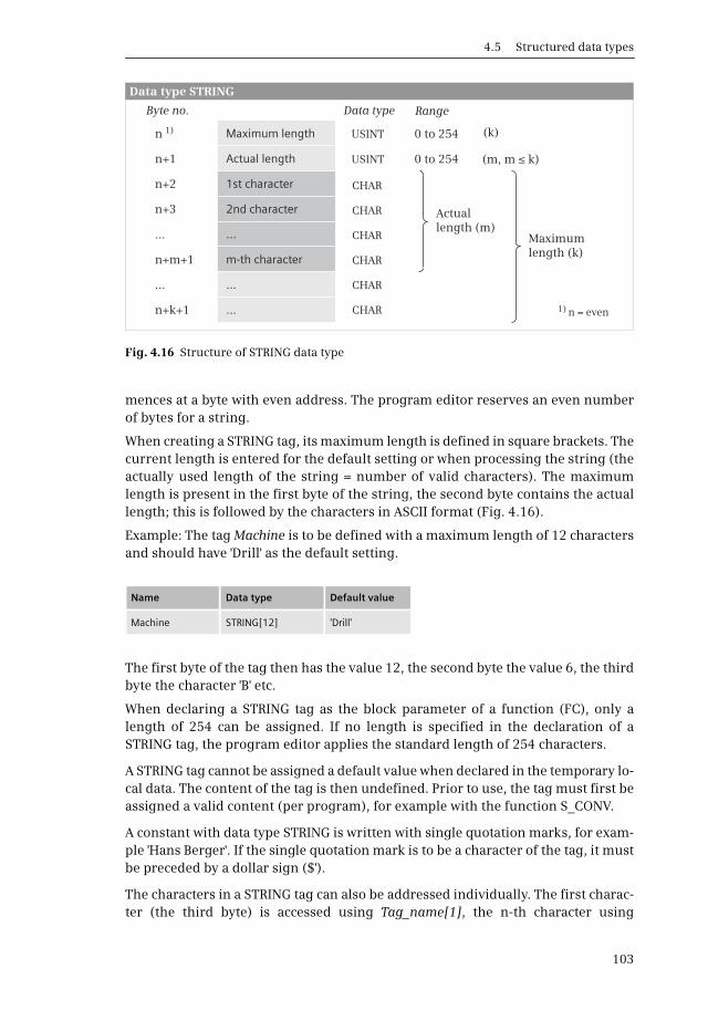
4.5 Structured data types
103
mences at a byte with even address. The program editor reserves an even numberof bytes for a string.
When creating a STRING tag, its maximum length is defined in square brackets. Thecurrent length is entered for the default setting or when processing the string (theactually used length of the string = number of valid characters). The maximumlength is present in the first byte of the string, the second byte contains the actuallength; this is followed by the characters in ASCII format (Fig. 4.16).
Example: The tag Machine is to be defined with a maximum length of 12 charactersand should have 'Drill' as the default setting.
The first byte of the tag then has the value 12, the second byte the value 6, the thirdbyte the character 'B' etc.
When declaring a STRING tag as the block parameter of a function (FC), only alength of 254 can be assigned. If no length is specified in the declaration of aSTRING tag, the program editor applies the standard length of 254 characters.
A STRING tag cannot be assigned a default value when declared in the temporary lo-cal data. The content of the tag is then undefined. Prior to use, the tag must first beassigned a valid content (per program), for example with the function S_CONV.
A constant with data type STRING is written with single quotation marks, for exam-ple 'Hans Berger'. If the single quotation mark is to be a character of the tag, it mustbe preceded by a dollar sign ($').
The characters in a STRING tag can also be addressed individually. The first charac-ter (the third byte) is accessed using Tag_name[1], the n-th character using
Fig. 4.16 Structure of STRING data type
Name Data type Default value
Machine STRING[12] 'Drill'
n
n+1
n+2
n+3
...
n+m+1
...
n+k+1
(k)
(m, m ≤ k)
Actual length (m)
Maximum length (k)
Maximum length
Actual length
1st character
2nd character
...
m-th character
...
...
Data type STRING
n = even 1)
1) 0 to 254
0 to 254
RangeData type
USINT
USINT
CHAR
CHAR
CHAR
CHAR
CHAR
CHAR
Byte no.

4 Variables and data types
104
Tag_name[n]. The individual components have the data type CHAR. In the above ex-ample, the tag Machine[3] has the character 'h'.
Special functions are available for processing STRING tags, for example to separatea partial string or to combine two STRING tags into a single one (see Chapter 11.9“Processing of strings (Data type STRING)” on page 398).
4.5.3 Data type ARRAY
The data type ARRAY represents a data structure comprising a fixed number of com-ponents with the same data type Fig. 4.17). For the components, all data typesexcept ARRAY are permissible.
A tag with data type ARRAY commences at a word limit (at a byte with even address).Components with data type BOOL commence in the least significant bit; compo-nents with data type BYTE and CHAR in the right byte. The individual componentsare listed consecutively. The program editor reserves an even number of bytes for afield tag.
The data type ARRAY can have up to 65 536 components. When creating an ARRAYtag, the number range of the components is specified in square brackets, and thedata type following the keyword OF. The number range extends from –32 768 to32 767. The lower range value must be smaller than the upper value.
Example: A tag with the name Measured_value is to have 16 components of datatype INT which are numbered commencing with 1.
The components of an ARRAY tag can also be addressed individually, and can behandled like tags with the same data type. For example, the component Mea-sured_value[10] on a block parameter can be created with the data type INT.Addressing with a variable index is also possible: Measured_value[#var_index] (seeChapter 4.2.7 “Indirect addressing” Section “Indirect addressing of field compo-nents” on page 90).
4.5.4 Data type STRUCT
The STRUCT data type represents a data structure comprising a fixed number ofcomponents with different data types (Fig. 4.18). For the individual components, alldata types are permissible.
A tag with data type STRUCT commences at a word limit (at a byte with even ad-dress), followed by the components in the declared sequence. Components with the
Name Data type Start value
Measured_value ARRAY[1..16] OF INT
Measured_value[1] INT 0
Measured_value[2] INT 0
...
Measured_value[16] INT 0
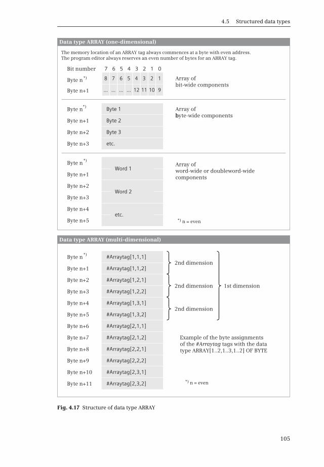
4.5 Structured data types
105
Fig. 4.17 Structure of data type ARRAY
Byte n
Byte n
Byte n
Bit number
Byte n+1
Byte n+1
Byte n+1
Byte n+2
Byte n+2
Byte n+3
Byte n+3
Byte n+4
Byte n+5
7 6 5 4 3 2 1 0
Array of bit-wide components
Array of byte-wide componentsb
Array of word-wide or doubleword-wide components
n = even
*)
*)
*)
*)
8
...
7
...
6
...
5
...
4
12
3
11
2
10
1
9
Byte 1
Byte 2
Byte 3
etc.
Word 1
Word 2
etc.
Byte n+4
Byte n
Byte n+5
Byte n+1
Byte n+6
Byte n+2
Byte n+7
Byte n+3
Byte n+8
Byte n+10
Byte n+9
Byte n+11
1st dimension2nd dimension
2nd dimension
n = even
*)
*)
Data type ARRAY (multi-dimensional)
#Arraytag[1,1,1]
#Arraytag[1,1,2]
#Arraytag[1,2,1]
#Arraytag[1,2,2]
#Arraytag[1,3,1]
#Arraytag[1,3,2]
#Arraytag[2,1,1]
#Arraytag[2,1,2]
#Arraytag[2,2,1]
#Arraytag[2,2,2]
#Arraytag[2,3,1]
#Arraytag[2,3,2]
Data type ARRAY (one-dimensional)
2nd dimension
Example of the byte assignments of the #Arraytag tags with the data type ARRAY[1..2,1..3,1..2] OF BYTE
The memory location of an ARRAY tag always commences at a byte with even address. The program editor always reserves an even number of bytes for an ARRAY tag.
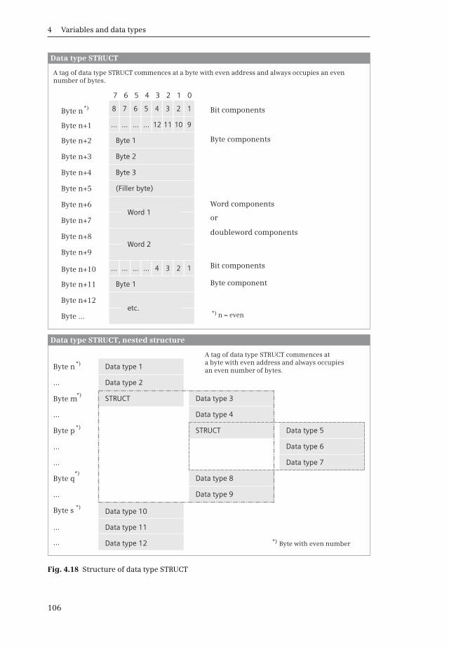
4 Variables and data types
106
Fig. 4.18 Structure of data type STRUCT
Byte n+6
Byte n+2
Byte n+11
Byte n
Byte n+7
Byte n+3
Byte n+1
Byte n+10
Byte n+8
Byte n+4
Byte n+9
Byte n+5
Byte n+12
Byte ...
7 6 5 4 3 2 1 0
Bit components
Bit components
Byte component
Byte components
Word components
or
doubleword components
n = even
*)
*)
8
...
...
7
...
...
6
...
...
5
...
...
4
12
4
3
11
3
2
10
2
1
9
1
Byte 1
Byte 1
Byte 2
Byte 3
(Filler byte)
Word 1
Word 2
etc.
Data type STRUCT
…
Byte m
…
Byte n
Byte q
…
…
…
…
Byte p
Byte s
…
*)
*)
*)
*)
*) STRUCT
STRUCT
Data type 7
Data type 1
Data type 3
Data type 8
Data type 10
Data type 12
Data type 5
Data type 2
Data type 4
Data type 9
Data type 11
Data type 6
Data type STRUCT, nested structure
Byte with even number*)
A tag of data type STRUCT commences at a byte with even address and always occupies an even number of bytes.
A tag of data type STRUCT commences at a byte with even address and always occupies an even number of bytes.

4.6 Parameter types
107
data type BOOL commence in the least significant bit of the next vacant byte, com-ponents with the data type BYTE or CHAR in the next vacant byte. Components withother data types commence at a word limit. The program editor reserves an evennumber of bytes for a STRUCT tag.
When declaring a STRUCT tag, the tag name with the STRUCT data type is specifiedfirst, followed underneath by the individual components with their own data type.
Example: A tag with the name Fan is to comprise four components: “Switch on fan”(BOOL), “Switch off fan” (BOOL), “Speed” (INT) and “Delay” (TIME).
A component of a STRUCT tag can also be addressed individually by positioning thename of the structure, separated by a dot, in front of the component name.A STRUCT component can be handled like a tag with the same data type. For exam-ple, the component Fan.Speed on a block parameter can be created with the datatype INT.
4.6 Parameter types
The parameter types are additional data types for block parameters. The parametertypes comprise, for example, the data types for the transfer of IEC timer functionsand IEC counter functions, the transfer of any tags, and the data type for the func-tion value of a function. PLC data types, system data types, and hardware data typescan be used for the block parameters.
4.6.1 Parameter types for IEC timer functions
The following data types are available for the transfer of IEC timer functions to theblock interface:
Name Data type Start value
Fan STRUCT
Switch on fan BOOL false
Switch off fan BOOL false
Speed INT 0
Delay TIME T#0ms
Timer function Data type of the duration IEC data type
Pulse generation TIME TP_TIME
ON delay TIME TON_TIME
OFF delay TIME TOF_TIME
Accumulating ON delay TIME TONR_TIME

4 Variables and data types
108
The structure of the data types corresponds to the structure of the system data typeIEC_TIMER (see Chapter 4.8.1 “IEC_TIMER system data type” on page 110).
The data types can be used in the declaration sections Input (input parameters),InOut (in-out parameters), and Static (static local data). If an IEC timer function istransferred as input parameter, its components can only be scanned. You supply ablock parameter with the data type of an IEC timer function with the name of theinstance data, either with the data block if the call is created as a single instance, orwith the instance name if the call is created as a local instance in a function block.
The data types for IEC timer functions can also be used in PLC data types.
4.6.2 Parameter types for IEC counter functions
Depending on the counter type and the data type of the count value, there are thefollowing data types for the transfer of IEC counter functions to the block interface:
The structure of the data types corresponds to the structure of the system data typeIEC_xCOUNTER (see Chapter 4.8.2 “IEC_COUNTER system data type” on page 112).
The data types can be used in the declaration sections Input (input parameters),InOut (in-out parameters), and Static (static local data). If an IEC counter functionis transferred as input parameter, its components can only be scanned. You supplya block parameter with the data type of an IEC counter function with the name ofthe instance data, either with the data block if the call is created as a single instance,or with the instance name if the call is created as a local instance in a function block.
The data types for IEC counter functions can also be used in PLC data types.
4.6.3 Parameter type VARIANT
A block parameter with data type VARIANT contains a pointer to a tag or a data area.Tags of all data types are approved for a block parameter of type VARIANT. The tags(operands or data types) which can be connected to the block parameter or whichare meaningful are defined by the program within the called block.
Counter type Data type of the count value
IEC data type
Up counter SINTINTDINT
CTU_SINTCTU_INTCTU_DINT
Down counter SINTINTDINT
CTD_SINTCTD_INTCTD_DINT
Up/down counter SINTINTDINT
CTUD_SINTCTUD_INTCTUD_DINT
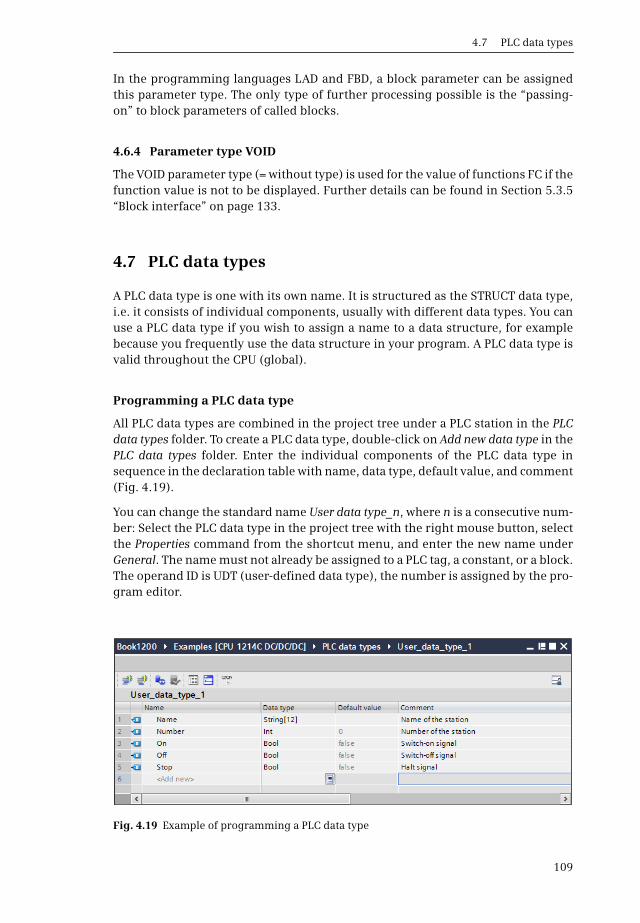
4.7 PLC data types
109
In the programming languages LAD and FBD, a block parameter can be assignedthis parameter type. The only type of further processing possible is the “passing-on” to block parameters of called blocks.
4.6.4 Parameter type VOID
The VOID parameter type (= without type) is used for the value of functions FC if thefunction value is not to be displayed. Further details can be found in Section 5.3.5“Block interface” on page 133.
4.7 PLC data types
A PLC data type is one with its own name. It is structured as the STRUCT data type,i.e. it consists of individual components, usually with different data types. You canuse a PLC data type if you wish to assign a name to a data structure, for examplebecause you frequently use the data structure in your program. A PLC data type isvalid throughout the CPU (global).
Programming a PLC data type
All PLC data types are combined in the project tree under a PLC station in the PLCdata types folder. To create a PLC data type, double-click on Add new data type in thePLC data types folder. Enter the individual components of the PLC data type insequence in the declaration table with name, data type, default value, and comment(Fig. 4.19).
You can change the standard name User data type_n, where n is a consecutive num-ber: Select the PLC data type in the project tree with the right mouse button, selectthe Properties command from the shortcut menu, and enter the new name underGeneral. The name must not already be assigned to a PLC tag, a constant, or a block.The operand ID is UDT (user-defined data type), the number is assigned by the pro-gram editor.
Fig. 4.19 Example of programming a PLC data type

4 Variables and data types
110
Using a PLC data type
A PLC data type can be assigned to any tag which is present in a global data blockor in the interface of a logic block. The default setting for the PLC data type canbe changed. You then address the individual components of the tag using#var_name.comp_name (Fig. 4.20).
With a PLC data type as the basis, you can also generate a data block: In the projecttree, double-click on Add new block in the Program blocks folder. Click on the Datablock button in the Add new block window, and select the PLC data type from theType drop-down list. The data structure of this type data block is then defined bythe PLC data type and can no longer be changed. The default setting is importedby the PLC data type and can be changed.
4.8 System data types
System data types (SDT) are predefined data types which – like the data typeSTRUCT – consist of a fixed number of components each with different elementarydata types. System data types are delivered together with STEP 7 and cannot bemodified.
The system data types can only be used together with certain functions or state-ments. Table 4.7 shows a selection of system data types.
4.8.1 IEC_TIMER system data type
The instance data of an IEC timer function is structured according to the systemdata type IEC_TIMER. If you use the instructions TP, TON, TOF, or TONR, theprogram editor – depending on the specification Single instance or Multi-instance –
Fig. 4.20 Example of application of a PLC data type
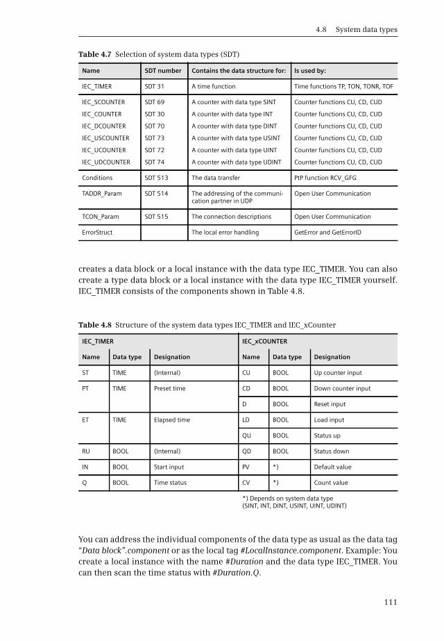
4.8 System data types
111
creates a data block or a local instance with the data type IEC_TIMER. You can alsocreate a type data block or a local instance with the data type IEC_TIMER yourself.IEC_TIMER consists of the components shown in Table 4.8.
You can address the individual components of the data type as usual as the data tag“Data block”.component or as the local tag #LocalInstance.component. Example: Youcreate a local instance with the name #Duration and the data type IEC_TIMER. Youcan then scan the time status with #Duration.Q.
Table 4.7 Selection of system data types (SDT)
Name SDT number Contains the data structure for: Is used by:
IEC_TIMER SDT 31 A time function Time functions TP, TON, TONR, TOF
IEC_SCOUNTER SDT 69 A counter with data type SINT Counter functions CU, CD, CUD
IEC_COUNTER SDT 30 A counter with data type INT Counter functions CU, CD, CUD
IEC_DCOUNTER SDT 70 A counter with data type DINT Counter functions CU, CD, CUD
IEC_USCOUNTER SDT 73 A counter with data type USINT Counter functions CU, CD, CUD
IEC_UCOUNTER SDT 72 A counter with data type UINT Counter functions CU, CD, CUD
IEC_UDCOUNTER SDT 74 A counter with data type UDINT Counter functions CU, CD, CUD
Conditions SDT 513 The data transfer PtP function RCV_GFG
TADDR_Param SDT 514 The addressing of the communi-cation partner in UDP
Open User Communication
TCON_Param SDT 515 The connection descriptions Open User Communication
ErrorStruct The local error handling GetError and GetErrorID
Table 4.8 Structure of the system data types IEC_TIMER and IEC_xCounter
IEC_TIMER IEC_xCOUNTER
Name Data type Designation Name Data type Designation
ST TIME (Internal) CU BOOL Up counter input
PT TIME Preset time CD BOOL Down counter input
D BOOL Reset input
ET TIME Elapsed time LD BOOL Load input
QU BOOL Status up
RU BOOL (Internal) QD BOOL Status down
IN BOOL Start input PV *) Default value
Q BOOL Time status CV *) Count value
*) Depends on system data type (SINT, INT, DINT, USINT, UINT, UDINT)

4 Variables and data types
112
4.8.2 IEC_COUNTER system data type
The instance data of an IEC counter function is structured depending on thedata type of the counter value according to the system data types C_SCOUNTER(SINT data type), IEC_COUNTER (INT), IEC_DCOUNTER (DINT), IEC_US_COUNTER(USINT), IEC_UCOUNTER (UINT), and IEC_UDCOUNTER (UDINT).
If you use one of the statements CTU, CTD, or CTUD, the program editor – depend-ing on the specification Single instance or Multi-instance – creates a data block or alocal instance with the data type IEC_xCOUNTER. You can also create a type datablock or a local instance with the data type IEC_xCOUNTER yourself. IEC_xCOUNTERconsists of the components shown in Table 4.8.
You can address the individual components of the data type as usual as the data tag“Data block”.component or as the local tag #LocalInstance.component. Example: Youcreate a local instance with the name Number and the data type IEC_COUNTER. Youcan then scan the count value with #Number.CV.
4.8.3 TCON_Param data type
The data type TCON_Param contains the structure of the connection data either forthe communication connection to the partner device (TCP native and ISO-on-TCPprotocols) or for the connection to the communication access point of the localoperating system (UDP protocol). You require a data block with this structure foreach connection (Table 4.9).
4.8.4 TADDR_Param data type
The data type TADDR_Param contains the structure of the remote partner's addressinformation when using the UDP protocol. With this data structure you configure adata area in a data block which contains the addresses of the receiver stations andparameterize this data area at the ADDR parameter of the send block TUSEND. Atthe receive block TURCV you parameterize a data area with this structure at theADDR parameter which accommodates the addresses of the transmitting station(Table 4.10).
4.8.5 Data type ErrorStruct
The data type ErrorStruct is a data structure with predefined assignment. The datatype is used by the functions for error evaluation GetError and GetErrorID. Infor-mation concerning errors is output with this structure (Table 4.11). A tag with datatype ErrorStruct commences at a word limit (at a byte with even address).
Additional information is output depending on the assignment of the structurecomponent MODE (Table 4.12). When declaring an ErrorStruct tag, the data type isselected from the drop-down list. The components can also be addressed individu-ally: Tag_name.Component_name.

4.8 System data types
113
Table 4.9 Structure of data type TCON_Param
Byte Parameter Data type Description
0 and 1 block_length WORD Length of TCON_PAR (fixed at 64 bytes)
2 and 3 id WORD Connection ID
4 connection_type BYTE Protocol variantB#16#11: TCPB#16#12: ISO-on-TCPB#16#13: TCP (compatibility mode)
With UDP: B#16#13
5 active_est BOOL Type of connection establishmentFALSE: Passive connection establishmentTRUE: Active connection establishment
With UDP: FALSE
6 local_device_id BYTE Communication module ID
7 local_tsap_id_len BYTE Length of parameter local_tsap_id
8 rem_subnet_id_len BYTE B#16#00
9 rem_staddr_len BYTE Length of parameter rem_staddr
With UDP: B#16#00
10 rem_tsap_id_len BYTE Length of parameter rem_tsap_id
With UDP: B#16#00
11 next_staddr_len BYTE Length of parameter next_staddr
With UDP: B#16#00
12to27 local_tsap_id ARRAY [1..16] OF BYTE Depending on connection:local port number or local TSAP ID
With UDP: local port number
28to33 rem_subnet_id ARRAY [1..6] OF BYTE B#16#00
34to39 rem_staddr ARRAY [1..6] OF BYTE IP address of remote partner
With UDP: B#16#00
40to55 rem_tsap_id ARRAY [1..16] OF BYTE Depending on connection:remote port number or remote TSAP ID
With UDP: B#16#00
56to61 rem_staddr ARRAY [1..6] OF BYTE CP slot
With UDP: B#16#00
62 and 63 spare WORD W#16#0000
Table 4.10 Structure of data type TADDR_Param
Byte Parameter Data type Description
0to3 rem_ip_addr ARRAY [1..4] OF BYTE IP address of remote partner
4 and 5 rem_port_nr ARRAY [1..2] OF BYTE Port no. of remote partner
6 and 7 spare ARRAY [1..2] OF BYTE B#16#00

4 Variables and data types
114
Table 4.11 Structure of ErrorStruct data type
Name Data type Note, assignment
ERROR_ID WORD Error ID (see text)
FLAGS BYTE 16#00
REACTION BYTE Reactions to error16#00: none, no writing (write error)16#01: replace, read a zero (read error)16#02: skip statement (system error)
CODE_ADDRESS CREF
BLOCK_TYPE BYTE Type of block in which the error occurred16#01: OB, 16#02: FC, 16#03: FB
CODE_BLOCK_NUMBER UINT Number of block in which the error occurred
OFFSET UDINT Internal memory address at which the error occurred
MODE BYTE Assignment for the significance of the supplied data (A) to (E) (see text)
OPERAND_NUMBER UINT Internal operand number of operation
POINTER_NUMBER_LOCATION UINT Internal pointer address of operation (A) (see text)
SLOT_NUMBER_SCOPE UINT Internal address in memory (B) (see text)
DATA_ADDRESS NREF
AREA BYTE Addressed memory area on occurrence of error (C) (see text)
DB_NUMBER UINT Number of data block on occurrence of error, otherwise zero (D) (see text)
OFFSET UDINT Bit offset on occurrence of error (E) (see text)
Table 4.12 Information output depending on access type MODE
MODE (A) (B) (C) (D) (I)
16#00 – – – – –
16#01 – – – – OFFSET
16#02 – – AREA – –
16#03 LOCATION SCOPE – NUMBER –
16#04 – – AREA – OFFSET
16#05 – – AREA DB_NUMBER OFFSET
16#06 POINTER_NUMBER_LOCATION
SLOT_NUMBER_SCOPE
AREA DB_NUMBER OFFSET
16#07 POINTER_NUMBER_LOCATION
SLOT_NUMBER_SCOPE
AREA DB_NUMBER OFFSET
Memory area Assignment of AREA component
System memory (temporary local data)
16#40…4E, 16#86, 16#87, 16#8E, 16#8F, 16#C0…CE
Process image input (I) 16#81
Process image output (Q) 16#82
Bit memory (M) 16#83
Data operand (DB) 16#84, 16#85, 16#8A, 16#8B

4.9 Hardware data types
115
The assignment of the ERROR_ID and handling of the error evaluation is describedin Section 5.8.4 “Local error handling” on page 169.
4.8.6 TimeTransformationRule data type
The data type TimeTransformationRule contains the correction values for settingthe local time on the CPU (see Chapter 5.6.6 “Time” on page 148). It is requiredin conjunction with the SET_TIMEZONE function to calculate the local time fromthe module time (time data of the real-time clock) and to make the switchbetween daylight saving and standard time (Table 4.13).
4.9 Hardware data types
Hardware data types refer to all those which can accept the constants in the defaulttag table in the System constants tab. These constants are used to address hardwareand software objects in the program. The data type and the value are predefined,the name can be changed in the object properties.
Fig. 4.21 shows the System constants tab with a selection of hardware data types.
Table 4.13 Data structure for TimeTransformationRule
Byte Name Data type Note
0 Bias INT Correction value for the time zone to UTC in minutes
2 DaylightBias INT Correction value daylight saving/standard time in minutes
Beginning of daylight saving time :
4 DaylightStartMonth USINT Month
5 DaylightStartWeek USINT Week ( 1 = first in month)
6 DaylightStartWeekday USINT Weekday (1 = Sunday)
7 DaylightStartHour USINT Hour
8 DaylightStartMinute USINT Minute
Beginning of standard time :
9 StandardStartMonth USINT Month
10 StandardStartWeek USINT Week ( 1 = first in month)
11 StandardStartWeekday USINT Weekday (1 = Sunday)
12 StandardStartHour USINT Hour
13 StandardStartMinute USINT Minute
14 TimeZoneName STRING[80] Name of time zone, e.g. ’(GMT +01:00) Amsterdam, Berlin, Bern, Rome, ...’
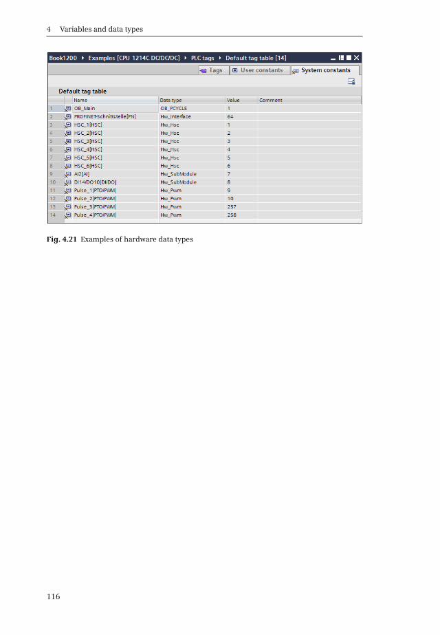
4 Variables and data types
116
Fig. 4.21 Examples of hardware data types
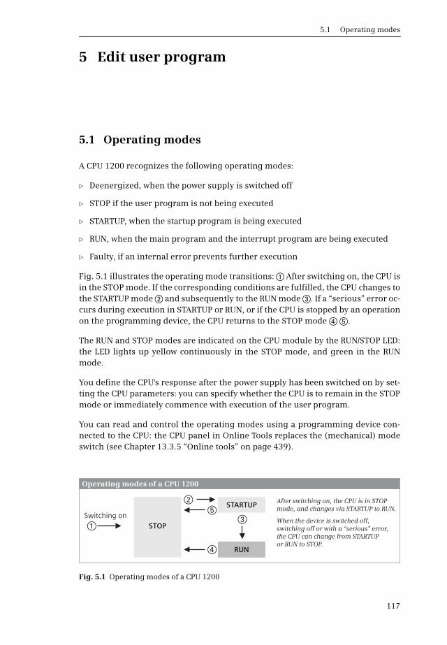
5.1 Operating modes
117
5 Edit user program
5.1 Operating modes
A CPU 1200 recognizes the following operating modes:
b Deenergized, when the power supply is switched off
b STOP if the user program is not being executed
b STARTUP, when the startup program is being executed
b RUN, when the main program and the interrupt program are being executed
b Faulty, if an internal error prevents further execution
Fig. 5.1 illustrates the operating mode transitions: a After switching on, the CPU isin the STOP mode. If the corresponding conditions are fulfilled, the CPU changes tothe STARTUP mode s and subsequently to the RUN mode d. If a “serious” error oc-curs during execution in STARTUP or RUN, or if the CPU is stopped by an operationon the programming device, the CPU returns to the STOP mode f g.
The RUN and STOP modes are indicated on the CPU module by the RUN/STOP LED:the LED lights up yellow continuously in the STOP mode, and green in the RUNmode.
You define the CPU's response after the power supply has been switched on by set-ting the CPU parameters: you can specify whether the CPU is to remain in the STOPmode or immediately commence with execution of the user program.
You can read and control the operating modes using a programming device con-nected to the CPU: the CPU panel in Online Tools replaces the (mechanical) modeswitch (see Chapter 13.3.5 “Online tools” on page 439).
Fig. 5.1 Operating modes of a CPU 1200
STOP
STARTUP
RUN
Switching onWhen the device is switched off, switching off or with a “serious” error, the CPU can change from STARTUP or RUN to STOP.
After switching on, the CPU is in STOP mode, and changes via STARTUP to RUN.
Operating modes of a CPU 1200

5 Edit user program
118
5.1.1 STOP mode
The STOP mode is reached:
b When the CPU is switched on
b If a “serious” error occurs
b If the STP system function is executed
b If a stop request arrives from the programming device
The CPU enters the cause of the STOP operating mode into the diagnostics buffer.In this operating mode, you can also read out the CPU information using a pro-gramming device in order to find the reason for the stop.
The user program is not executed in STOP mode. The CPU takes over the device set-tings – either the values you have set with the hardware configuration when param-eterizing the CPU, or the standard settings – and sets the connected modules to theparameterized initial state.
In the STOP mode, the CPU can passively execute one-way communication if, forexample, data is requested or sent by another CPU via S7 communication. The real-time clock continues to run in the STOP mode.
You can parameterize the CPU in the STOP operating mode, for example set the IPaddress, transfer or modify the user program, and you can also carry out a memoryreset for the CPU.
Disabling of output modules
All output modules are disabled when in the STOP and STARTUP operating modes(OD or BASP signal, output disable or disable command output). Disabled outputmodules output a zero signal or – if configured accordingly – a substitute value.
Although writing to the modules influences the signal memories on them, it doesnot switch the signal states “to the outside” to the module terminals. The outputmodules are only enabled when the RUN operating mode is reached.
In the STOP operating mode, you can cancel disabling of the output modules fortesting purposes (see Chapter 13.4.9 “Enable peripheral outputs and “Modify now””on page 451).
5.1.2 STARTUP mode
Before the CPU changes from the STOP mode to the RUN mode, it runs through theSTARTUP mode. In the STARTUP mode, the CPU initializes itself and the modulescontrolled by it. If the CPU detects an error in the STARTUP mode, e.g. if an invalidmemory card is inserted, it returns to the STOP mode.
You can define the startup response when parameterizing the CPU with the deviceconfiguration. With the CPU module selected in the Properties tab of the Inspectorwindow, click on Startup and select:

5.1 Operating modes
119
b No startup (stay in STOP mode)When the CPU is switched on, it remains in the STOP mode without executing the startup program.
b Warm restart – RUNAfter switching on, the CPU executes a warm restart. The values of the non-retentive tags are deleted. The startup program is then executed once before the CPU in the RUN mode cyclically executes the main program.
b Warm restart – mode prior to POWER OFFAfter the system has been switched on, the CPU starts the mode in which it was present prior to switching off (STOP or warm restart and RUN).
Warm restart
With a warm restart, the CPU sets itself and the modules to the configured basicstate. It deletes the non-retentive data in the system memory (inputs, outputs, bitmemories) and sets the non-retentive data tags to the start values from the loadmemory. The data set as retentive (bit memories, data tags) is retained.
CPU activities in STARTUP mode
In the STARTUP mode, the CPU first deletes the input process image and disablesthe peripheral outputs (Fig. 5.2). The signal states on the output modules are setduring this process according to their parameterization: retain last value or outputparameterized substitute value.
Startup organization blocks are called once if present. The input process image isupdated following execution of the startup program, and disabling of the peripher-al outputs is canceled.
No Open User Communication is carried out during the startup. The high-speedcounters (HSC), the pulse generators, and the point-to-point connections of theCM modules are not processed. The CPU updates the real-time clock.
If a restart is aborted by a power supply failure, for example, it is then re-executedfrom the beginning when the CPU is switched on again.
Further information on user program processing in the STARTUP state can befound in Chapter 5.5 “Start-up routine” on page 142.
5.1.3 RUN mode
The RUN mode is reached from the STARTUP mode. In the RUN mode, the PLC sta-tion controls the machine or process.
The following activities are executed cyclically by the CPU (see also Fig. 5.2):
b Transmission of output process image to the output modules
b Updating of input process image
b Execution of main program
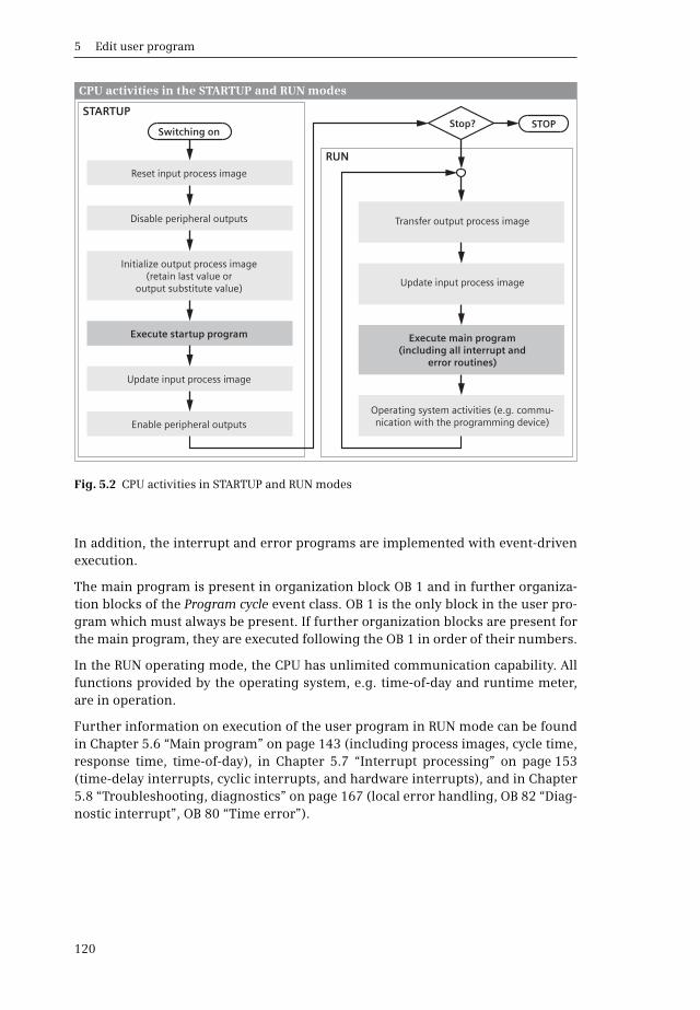
5 Edit user program
120
In addition, the interrupt and error programs are implemented with event-drivenexecution.
The main program is present in organization block OB 1 and in further organiza-tion blocks of the Program cycle event class. OB 1 is the only block in the user pro-gram which must always be present. If further organization blocks are present forthe main program, they are executed following the OB 1 in order of their numbers.
In the RUN operating mode, the CPU has unlimited communication capability. Allfunctions provided by the operating system, e.g. time-of-day and runtime meter,are in operation.
Further information on execution of the user program in RUN mode can be foundin Chapter 5.6 “Main program” on page 143 (including process images, cycle time,response time, time-of-day), in Chapter 5.7 “Interrupt processing” on page 153(time-delay interrupts, cyclic interrupts, and hardware interrupts), and in Chapter5.8 “Troubleshooting, diagnostics” on page 167 (local error handling, OB 82 “Diag-nostic interrupt”, OB 80 “Time error”).
Fig. 5.2 CPU activities in STARTUP and RUN modes
RUN
STARTUP
Switching onSTOPStop?
Operating system activities (e.g. commu-nication with the programming device)
Reset input process image
Update input process image
Disable peripheral outputs Transfer output process image
Enable peripheral outputs
Update input process image
Initialize output process image(retain last value or
output substitute value)
Execute startup program Execute main program(including all interrupt and
error routines)
CPU activities in the STARTUP and RUN modes
5.1 Operating modes
121
5.1.4 Retentive behavior of operands
A memory area is retentive if its contents are retained even when the power supplyis switched off, as well as on a transition from STOP to RUN following power-up. Theretentive memory of a CPU 1200 comprises 10 KB. It can accommodate bit memo-ries and data tags.
Retentivity settings for bit memories
You set the retentive memory area for the bit memories in the PLC tag table or inthe assignment list. Click on the Retain symbol in the toolbar of the working win-dow, and enter the number of retentive bytes. The retentive area starts at memorybyte 0 and ends at byte no. (number – 1). If a bit memory declaration is presentwithin this range, it is assigned a tick or the retentivity symbol in the “Retain” col-umn. A tag occupying more than one byte must not exceed the limit between theretentive and non-retentive ranges.
Retentivity settings for global data tags
If the Optimized block access attribute is activated in the global or type data block,individual tags can be defined as retentive. In the case of a tag with a structureddata type, only the complete tag can be set to retentive. If the attribute is not acti-vated, the retentive setting applies to the entire data block.
Retentivity settings for tags in function blocks
If the Optimized block access attribute is activated in a function block, the retentiv-ity of individual tags can be set in the interface area. Select the settings for each tagfrom a drop-down list:
b Non-retentiveThe tag in the instance data block is always non-retentive.
b RetentiveThe tag in the instance data block is always retentive.
b Set in IDBThe retentivity setting for the tag can be made in the instance data bock. The standard setting is “Non-retentive”.
For a tag with a structured data type, the retentivity setting applies for the wholetag.
If the attribute Optimized block access is not activated, the setting can be made inthe instance data block, but only for the complete data block. The Optimized blockaccess property of the function block is “bequeathed” to the associated instancedata blocks.

5 Edit user program
122
5.2 Creating a user program
5.2.1 Program draft
You define the structure of the user program already during the draft phase byadaptation to technological and functional conditions; this is important for pro-gram creation, testing, and commissioning. In order to achieve effective program-ming, it is therefore necessary to pay particular attention to the program structure.
Analysis of a complex automation task means division of it into smaller tasks orfunctions based on the structure of the process to be controlled. You define the in-dividual tasks by determining the function and then defining the interface signalsto the process or to other individual tasks. You can adopt this structuring of individ-ual tasks in your program. This means that the structure of your program corre-sponds to the structure of the automation task.
A structured user program is easier to configure and program section by section,and means that more than one person can carry out the work in the case of verylarge user programs. Last but not least, program testing, servicing, and mainte-nance are simplified by this division.
With a linear program structure, the entire user program is present in one singleblock – a good solution for small programs. The individual control functions areprogram parts within this block, and are executed in succession. A block with LADor FBD program is divided into so-called networks, each of which accommodatesone or more current paths or complete logic operations. STEP 7 numbers all net-works in succession. During editing and testing, you can directly reference eachnetwork using its number.
The networks are executed in order of their numbering, but can also be bypasseddepending on conditions. The program can be debugged in sections using jump in-structions temporarily inserted during commissioning.
A modular program structure is used if the task is very extensive, if you wish torepeatedly use program functions, or if complex tasks exist. Structuring meansdividing the program into sections (blocks) with self-contained functions or a func-tional correlation, and exchanging as few signals as possible with other blocks. Ifyou assign a specific (technological) function to each program section, manageableblocks are achieved with simple interfaces to other blocks.
Fig. 5.3 shows a comparison between the principles of linear and modular programstructuring using a simple example. With the linear program structure, the individ-ual control functions are written in succession into a block. In the modular pro-gram structure, each control function is present in a block which is called by a“higher” block. Further blocks can be called in turn in the called blocks.
Blocks can also be used repeatedly. Let us assume that the control of motors 1 to 3has the same function, only the input and output signals and the control operationsare different. A Motor block can then be called three times with different signals(parameters) and control the motors independent of one another.

5.2 Creating a user program
123
5.2.2 Program execution
The complete program of a CPU comprises the operating system and the user pro-gram.
The operating system is the totality of all statements and declarations of internaloperating functions (e.g. saving of data in event of power failure, activation of pri-ority classes etc.). The operating system is a fixed part of the CPU which you cannotmodify. However, you can reload the operating system from a memory card, e.g. fora program update.
The user program is the totality of all statements and declarations programmed byyou for signal processing by means of which the plant (process) to be controlled isinfluenced in accordance with the control task.
Fig. 5.3 Comparison between linear and modular program structures
Operating modes
Block callcommand
Operating modes
Control motor 1
Control motor 1
Control motor 2
Control motor 3
Control valve 1Control valve 1
Control valve 2Control valve 2
Display control Display control
Error evaluation Error evaluation
Data transfer Data transfer
Linearprogram structure
Main program Main program
Valve control
Motor control
Modular program structure
Control motor 2
Control motor 3
Linear and modular program structures

5 Edit user program
124
Program execution modes
The user program consists of program sections which are executed by the CPU forspecific events. These events can be, for example, the starting up of the automationsystem, an interrupt, or detection of a program error (Fig. 5.4). The programsassigned to the events are divided into priority classes which define the sequenceof program execution if several events occur simultaneously and thus the interruptcapability hierarchy.
The main program, which is executed cyclically by the CPU, has the lowest execu-tion priority. All other events can interrupt the main program following each state-ment; the CPU then executes the associated interrupt or error program and subse-quently returns to execution of the main program.
A specific organization block (OB) is assigned to each event. The organizationblocks represent the event classes in the user program. If an event occurs, the CPUcalls the associated organization block. An organization block is part of the userprogram which you can program yourself. There are organization blocks withpermanently assigned number and organization blocks with a freely assignablenumber.
Fig. 5.4 Program execution modes of a SIMATIC user program
Cycle start
Switching on
<Interrupt> Interruption
Interruption<Error>
Operating system
STARTUP mode
RUN mode
Startup program
Interrupt program
Error program
Main program
Control program
Program execution modes of the control program

5.3 Programming blocks
125
Program execution commences in the CPU with the startup program. A startupcan be triggered by switching on the power supply or by an operator input on a con-nected programming device. The startup program is optional. If you wish to createa startup program, use organization block OB 100. You can assign further user or-ganization blocks to the startup program. These are then executed in order of theirOB number following OB 100. Following execution of the startup program, theCPU commences with execution of the main program.
The main program is present as standard in organization block OB 1 which isalways executed by the CPU. The start of the program is identical to that of the firststatement in OB 1. You can assign further organization blocks to the cyclically exe-cuted main program. These user organization blocks are then executed in order oftheir OB number following OB 1. The main program represents the totality of allcyclically executed organization blocks.
Following execution of the main program, the CPU branches to the operating sys-tem and, following execution of various operating system functions (e.g. updateprocess images), calls OB 1 again and the user organization blocks assigned to themain program.
The events which can interrupt the main program are interrupts and errors.Interrupts come from the controlled plant (hardware interrupts), from the CPU(time-delay interrupts and cyclic interrupts), or from the modules (diagnostics in-terrupts). The errors include time error events.
The organization block OB 80 is used for processing a time error event; for the diag-nostic interrupt, there is the organization block OB 82. You can set the number ofthe other interrupt organization blocks yourself.
5.2.3 Nesting depth
The main program and the startup program have a maximum nesting depth of 16;an interrupt-controlled program has a nesting depth of 4. This means that begin-ning with an organization block (nesting depth 1), you can call another 15 or 3blocks arranged “horizontally” (nested). If more blocks are called, the CPU gener-ates a program execution error. The nesting depth is not changed if several blocksare called in succession (linear block calls).
5.3 Programming blocks
5.3.1 Block types
You can divide your program into individual sections as required. The STEP 7 pro-gramming languages support this program breakdown by providing the requiredstatements. The individual program sections should be program parts that are self-contained, each with a technological or functional correlation. These program parts

5 Edit user program
126
are called “blocks”. A block is a part of the user program that is defined by its func-tion, structure or application.
User blocks
In the case of comprehensive and complex programs, it is recommend and some-times necessary to “structure” (divide) the program in individual blocks. You canselect different types of block depending on the application:
b Organization blocks OBThe organization blocks represent the interface between operating system anduser program. The CPU's operating system calls the organization blocks whenspecific events occur, e.g. in the event of hardware or cyclic interrupts. The mainprogram is in organization block OB 1 by default. There are organization blockswith a fixed number and a specific assignment to events and organization blockswith one freely selectable assignment to events and freely selectable number.When calling, some organization blocks make so-called start information avail-able that can be evaluated in the user program.
b Function blocks FBA function block is part of the user program whose call can be programmed us-ing block parameters. A function block has a tag memory which is located in adata block. This data block is permanently assigned to the function block or, tobe more precise, to the function block call. It is possible to assign a different datablock (with the same data structure, but containing different values) to eachfunction block call. Such a permanently assigned data block is called an instancedata block, and the combination of function block call and instance data block isreferred to as a call instance, or “instance” for short. If a function block is calledas a single instance, a separate instance data block is assigned to the call. Whencalled as a local instance, the data is stored in the instance data block of the call-ing function block.
b Functions FCThe blocks referred to as “functions” are used to program frequently recurringautomation functions. The calls can be parameterized. Functions do not store in-formation, and have no assigned data block.
b Data blocks DBData blocks contain data of the user program. A data block can be generated as aglobal data block, as an instance data block, or as a type data block. With a globaldata block, you program the data tags directly in the data block. With an instancedata block, the programming of the assigned function block determines the datatags present in the data block, and a type data block has the structure of a PLCdata type.
The number of organization blocks and the block number are partially defined bythe operating system. You can freely assign the numbers of the freely assignableorganization blocks and the other blocks within the permissible ranges (OB from123 to 65 535, FC and FB from 0 to 65 535, DB from 1 to 65 535).
5.3 Programming blocks
127
For our small program structure example (Fig. 5.3 on page 123) we can nowroughly assign the block types to the individual control functions: the main pro-gram is present in organization block OB 1, either completely with the linear pro-gram structure or as block calls with the modular program structure. The individ-ual control functions are either present in functions FC if they need not save theirown data, or in function blocks FB when saving their own data.
The motors could be controlled by a function block Motor which is called with dif-ferent parameter assignments for the individual motors. The same applies to con-trol of the valves.
Finally, a global data block which is not assigned to a function block can collect thedata produced during program execution. The block Data transmission then con-tains the program which transfers the data to another controller.
System blocks
System blocks are components of the operating system. They can contain programs(system functions SFC or system function blocks SFB) or data (system data blocksSDB). System blocks make a number of important system functions accessible toyou, such as manipulating the internal CPU clock, or communications functions.Some of the functions offered under the extended statements in the program ele-ments catalog are system functions or system function blocks.
You can call system functions and system function blocks, but you cannot modifythem or program them yourself. The blocks themselves do not require space in theuser memory; only the block call and the instance data blocks of the system func-tion blocks are in the user memory.
System data blocks contain information on such things as the configuration of theautomation system or the parameterization of the modules. These blocks are gen-erated and managed by STEP 7 itself. You determine the contents of the system datablocks, for example, when you configure a station. As a rule, system data blocks arelocated in the load memory. You cannot access the contents of system data blocks.
The system blocks also include the technological function blocks (FBT). For exam-ple, the technological object Axis is implemented as a technological functionblock. The blocks themselves do not require space in the user memory; only theblock call and the instance data block of a technological function block are in theuser memory.
Standard blocks
In addition to the functions and function blocks you create yourself, off-the-shelfblocks are also available from Siemens. These so-called standard blocks can be pro-vided on a data medium or are delivered together with STEP 7, as extended state-ments or in the global libraries, for example. You cannot view or edit the range ofstandard blocks. Standard blocks behave like user blocks: they require space in theuser memory.

5 Edit user program
128
Standard blocks also share the number range with the user blocks. If a standardblock is added to the user program by means of an extended statement, for exam-ple, the number of the standard block can no longer be occupied by a user block. Ifa user block is already present with the number of the standard block which you addto the user program, the number of the standard block is initially retained. Thestandard block is then assigned a different, unused number during the next com-pilation.
5.3.2 Editing block properties
To display and change the block properties, select the block in the project tree andthen the Properties command in the shortcut menu. Fig. 5.5 shows examples of theblock properties: the General section of a hardware interrupt organization block,and the Information section of a function block.
The General section contains the Name of the block. The block name must beunique within the program and must not already have been assigned to anotherblock, a PLC tag, a constant, or a PLC data type. The name can contain letters, dig-its, and special characters (but not quotation marks). No distinction is madebetween upper and lower case when checking the name. The Type is determinedwhen creating the block. The number is the block number within the block type.The programming language is LAD, FBD, or SLC for blocks with programs, or DB fordata blocks.
Fig. 5.5 Block properties: OB tab “General” and FB tab “Information”
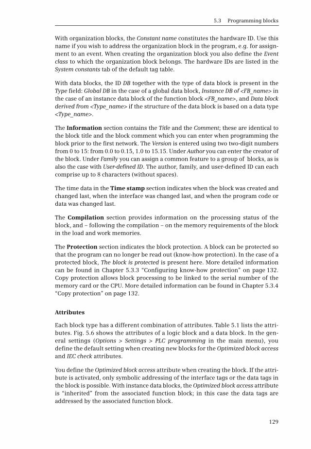
5.3 Programming blocks
129
With organization blocks, the Constant name constitutes the hardware ID. Use thisname if you wish to address the organization block in the program, e.g. for assign-ment to an event. When creating the organization block you also define the Eventclass to which the organization block belongs. The hardware IDs are listed in theSystem constants tab of the default tag table.
With data blocks, the ID DB together with the type of data block is present in theType field: Global DB in the case of a global data block, Instance DB of <FB_name> inthe case of an instance data block of the function block <FB_name>, and Data blockderived from <Type_name> if the structure of the data block is based on a data type<Type_name>.
The Information section contains the Title and the Comment; these are identical tothe block title and the block comment which you can enter when programming theblock prior to the first network. The Version is entered using two two-digit numbersfrom 0 to 15: from 0.0 to 0.15, 1.0 to 15.15. Under Author you can enter the creator ofthe block. Under Family you can assign a common feature to a group of blocks, as isalso the case with User-defined ID. The author, family, and user-defined ID can eachcomprise up to 8 characters (without spaces).
The time data in the Time stamp section indicates when the block was created andchanged last, when the interface was changed last, and when the program code ordata was changed last.
The Compilation section provides information on the processing status of theblock, and – following the compilation – on the memory requirements of the blockin the load and work memories.
The Protection section indicates the block protection. A block can be protected sothat the program can no longer be read out (know-how protection). In the case of aprotected block, The block is protected is present here. More detailed informationcan be found in Chapter 5.3.3 “Configuring know-how protection” on page 132.Copy protection allows block processing to be linked to the serial number of thememory card or the CPU. More detailed information can be found in Chapter 5.3.4“Copy protection” on page 132.
Attributes
Each block type has a different combination of attributes. Table 5.1 lists the attri-butes. Fig. 5.6 shows the attributes of a logic block and a data block. In the gen-eral settings (Options > Settings > PLC programming in the main menu), youdefine the default setting when creating new blocks for the Optimized block accessand IEC check attributes.
You define the Optimized block access attribute when creating the block. If the attri-bute is activated, only symbolic addressing of the interface tags or the data tags inthe block is possible. With instance data blocks, the Optimized block access attributeis “inherited” from the associated function block; in this case the data tags areaddressed by the associated function block.

5 Edit user program
130
The Optimized block access attribute results in “optimized” storage of the tags: thetags are not stored in the declaration sequence but are “packed together”, i.e. bitand byte tags are combined when possible in 16-bit packages. The Optimized blockaccess attribute also has effects on the retentivity setting of the data variables: withthe attribute activated, individual variables can be set as retentive (in the associ-ated function block for instance data blocks), but only the complete block can be setwhen the attribute is not activated.
The IEC check attribute indicates how strict the data type test is to be in the logicblock. With the attribute not activated, it is usually sufficient if the variables usedhave the data width required for execution of the function or instruction; with theattribute activated, the data types of the variables must correspond to the requireddata types.
Table 5.1 Block attributes
Attribute In block Meaning with attribute activated
Optimized block access OB, 1)FB, FC, DB
The block parameters and local data or data tags can only be symbolically addressed; the retentivity can be set for individ-ual tags; the data type LREAL can be used.
IEC check OB, FB, FC With comparison and arithmetic statements, the data types of the tags must agree.
Handle errors within block OB, FB, FC One of the functions GetError or GetErrorID is programmed in the block; the system response to an error in the block is sus-pended.
Only store in load memory Global and type DBs
The data block is not transferred to the work memory (for future extensions).
Data block write-protected in the device
Global and type DBs
The values of the data tags cannot be overwritten by means of a program.
1) The attribute is always activated for an organization block
Fig. 5.6 Block properties: attributes of code and data blocks
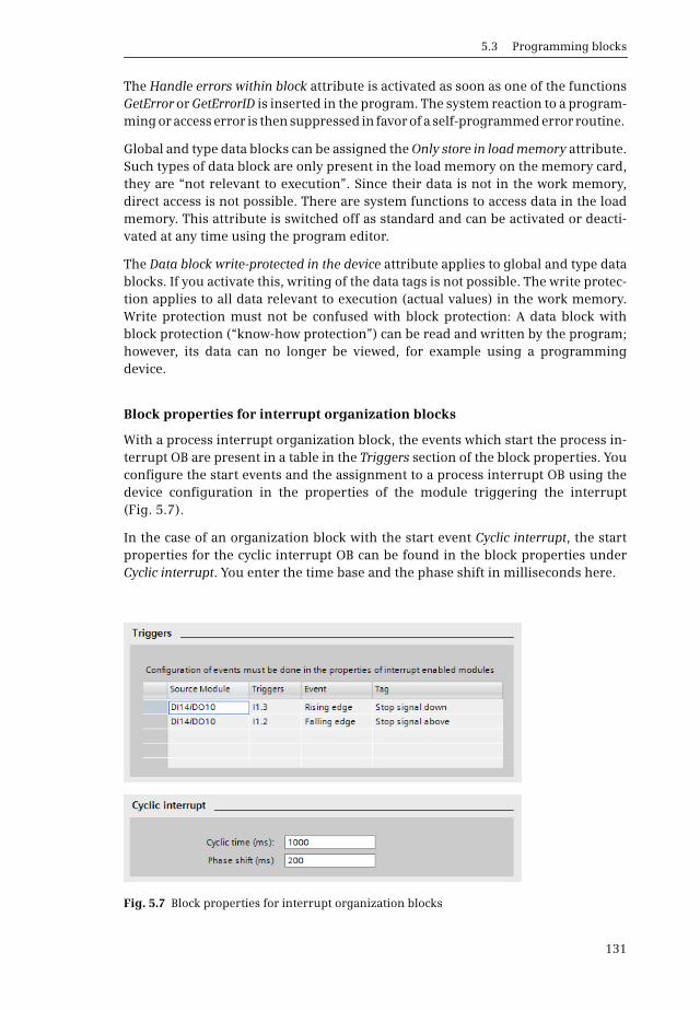
5.3 Programming blocks
131
The Handle errors within block attribute is activated as soon as one of the functionsGetError or GetErrorID is inserted in the program. The system reaction to a program-ming or access error is then suppressed in favor of a self-programmed error routine.
Global and type data blocks can be assigned the Only store in load memory attribute.Such types of data block are only present in the load memory on the memory card,they are “not relevant to execution”. Since their data is not in the work memory,direct access is not possible. There are system functions to access data in the loadmemory. This attribute is switched off as standard and can be activated or deacti-vated at any time using the program editor.
The Data block write-protected in the device attribute applies to global and type datablocks. If you activate this, writing of the data tags is not possible. The write protec-tion applies to all data relevant to execution (actual values) in the work memory.Write protection must not be confused with block protection: A data block withblock protection (“know-how protection”) can be read and written by the program;however, its data can no longer be viewed, for example using a programmingdevice.
Block properties for interrupt organization blocks
With a process interrupt organization block, the events which start the process in-terrupt OB are present in a table in the Triggers section of the block properties. Youconfigure the start events and the assignment to a process interrupt OB using thedevice configuration in the properties of the module triggering the interrupt(Fig. 5.7).
In the case of an organization block with the start event Cyclic interrupt, the startproperties for the cyclic interrupt OB can be found in the block properties underCyclic interrupt. You enter the time base and the phase shift in milliseconds here.
Fig. 5.7 Block properties for interrupt organization blocks

5 Edit user program
132
5.3.3 Configuring know-how protection
With the know-how protection for a block you can prevent a program or its datafrom being read out or modified. A protected block is identified in the project treeby a padlock icon. It is still possible to read the following from a block provided withknow-how protection:
b Block properties
b The parameters of the block interface
b Program structure
b Global tags (listed in the cross-reference list without specification of the position of use)
The following actions are still possible:
b Modify name and number in the block properties (necessary for copying and pasting the block)
b Copy and paste block where the know-how protection is also copied
b Delete, compile, and download block
b Call block (FB or FC) in the program of another block
b Compare online and offline versions of the block (comparison only of non-protected data).
To edit the know-how protection, select the block in the project tree under Programblocks, and then select Edit > Know-how protection in the main menu. To configurethe know-how protection, click the Define button, enter a password, confirm thepassword, and close the dialog with OK. To change the password, click the Changebutton, enter the old and new passwords, confirm the new password, and close thedialog with OK. To cancel the know-how protection, deactivate the Hide code (know-how protection) checkbox, enter the password, and close the dialog with OK.
You can also apply the know-how protection to several blocks simultaneously ifthese have the same password. If a function block is protected, the protection is“inherited” by the instance data block when calling as a single instance.
Note: If the password is lost, no further access to the block is possible. You can onlycancel the know-how protection of a block in its offline version. If you download acompiled block to the CPU, the recovery information is lost. A protected block whichyou have uploaded from the CPU cannot be opened, not even with the correct pass-word.
5.3.4 Copy protection
If a block has copy protection, processing of the block is dependent on a specificCPU or memory card. So that the copy protection cannot be removed, the blockmust then be provided with the know-how protection.
When the copy protection is being set up, the know-how protection for the blockmust be switched off. To set up the copy protection, select the block in the project

5.3 Programming blocks
133
tree, select Properties from the shortcut menu and then Protection. In the Copy pro-tection area, you can choose:
b No bindingNo copy protection is set or a set copy protection is canceled.
b Bind to serial number of the memory cardThe block can only be executed if the memory card has the specified serial number.
b Bind to serial number of the CPUThe block can only be executed if the CPU has the specified serial number.
To enter the serial number, the options Serial number is inserted when downloadingto a device or a memory card and Enter serial number are available with an input fieldfor the serial number.
5.3.5 Block interface
Components of the block interface
The block interface contains the declarations of the local tags that are used solelywithin the block. With the organization blocks (OB), these are – if present – the startinformation and the temporary local data. With function blocks (FB) and functions(FC), these are the block parameters which, when the block is called, provide the
Table 5.2 Declaration sections in the block interface
Section Data type Type, function Included in
Input E, Z, V, P, S, H
STRING[ ]STRING
Input parametersmay only be read in the program of the block
Data type STRING of any lengthData type STRING with the standard length of 254 characters
FC, FB and some OBs
FBFC
Output E, Z, P, (V)
STRING[ ]STRING
Output parametersmay only be written in the program of the blockData type STRING of any lengthData type STRING with the standard length of 254 characters
FC and FB
FBFC
InOut E, Z, P, V, S
STRING
In/out parametersmay be read and written in the program of the blockData type STRING with the standard length of 254 characters
FC and FB
FC and FB
Temp E, Z, P, STRING
Temporary local datais only valid during the current block processing
FC, FB and OB
Static E, Z, P, S Static local datais saved in the instance data block, and remains valid following block processing
FB
Return E, DTL, STRING, P, (V), VOID
Function valueOutput parameters with the return value of the function (not relevant to LAD and FBD)
FC
E = elementary data type, Z = structured data type (except STRING), P = PLC data typeV = parameter type VARIANT, (V) parameter type VARIANT only in functions FC S = system data type, H = hardware data type;FC = function, FB = function block, OB = organization block
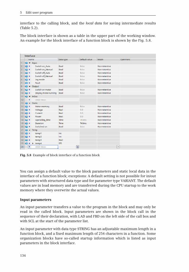
5 Edit user program
134
interface to the calling block, and the local data for saving intermediate results(Table 5.2).
The block interface is shown as a table in the upper part of the working window.An example for the block interface of a function block is shown by the Fig. 5.8.
You can assign a default value to the block parameters and static local data in theinterface of a function block; exceptions: A default setting is not possible for in/outparameters with structured data type and for parameter type VARIANT. The defaultvalues are in load memory and are transferred during the CPU startup to the workmemory where they overwrite the actual values.
Input parameters
An input parameter transfers a value to the program in the block and may only beread in the called block. Input parameters are shown in the block call in thesequence of their declaration, with LAD and FBD on the left side of the call box andwith SCL at the start of the parameter list.
An input parameter with data type STRING has an adjustable maximum length in afunction block, and a fixed maximum length of 254 characters in a function. Someorganization blocks have so-called startup information which is listed as inputparameters in the block interface.
Fig. 5.8 Example of block interface of a function block
5.3 Programming blocks
135
Output parameters
An output parameter transfers a value to the calling block and may only be writtenin the called block. Output parameters are shown in the block call in the sequenceof their declaration, with LAD and FBD on the right side of the call box and with SCLfollowing the input parameters in the parameter list.
An output parameter with data type STRING has an adjustable maximum length ina function block, and a fixed maximum length of 254 characters in a function.
Caution: Output parameters which cannot be assigned a default value must be writ-ten in the block during each block processing. This applies, for example, to all out-put parameters for a function (FC) and thus also to the function value. Note: Set andreset statements do not execute an action if the result of the logic operation = “0”,and therefore do not write to an output parameter!
In/out parameters
An in/out parameter transfers a value to the program in the block and can return itto the calling block, usually with a changed content. An in/out parameter can beread and written in the called block. In/out parameters are shown in the block callin the sequence of their declaration, with LAD and FBD on the left side of the callbox under the input parameters and with SCL at the end of the parameter list.
An in/out parameter with data type STRING has a fixed maximum length of 254characters.
Function value
The function value for functions is an output parameter which is handled in a spe-cial manner. It has the name Ret_Val with the declaration RETURN and the data typeVOID (= no type) as standard. The function value is used with the text-based pro-gramming language SCL (Structured Control Language). It is possible here to linkself-written functions in formulae (in expressions). The function value then corre-sponds to the value used for calculation in the formula.
With LAD and FBD you can ignore the function value in the interface description. Itis not indicated at the call box if the data type VOID is set. You can also assign a dif-ferent name and a different data type to the function value, and this is then dis-played as the first output parameter. In the program of the called block, you thentreat the function value in the same way as an output parameter.
Temporary local data
Temporary local data is stored in the system memory of the CPU. This data isaddressed symbolically and is only available during block processing. It is not dis-played on the call box or in the parameter list of the call statement. Further infor-mation can be found in Chapter 4.1.5 “Operand area temporary local data” onpage 85.

5 Edit user program
136
Static local data
The static local data is stored in the instance data of the called function block. It canbe read and written in the program of the called block. Static local data is addressedsymbolically. It retains its value until written again. It is not displayed on the callbox or in the parameter list of the call statement.
The static local data is usually only processed in the function block itself. However,since the static local data is saved in a data block, you can access it at any time liketags in a global data block using “Data block name”.tag name.
The static local data is normally accessed symbolically. Absolute addressing is onlypossible if the Optimized block access attribute is not activated in the function block– and thus also in the derived instance data block – and if you address the data oper-ands in the instance data block like the data operands of a global data block: using%Data block number.Data operand address, e.g. %DB12.DBW0.
5.3.6 Programming block parameters
By means of block parameters you enable parameterization of the processing spec-ification (the block function) present in a block.
Fig. 5.9 Example of programming with block parameters
Adder
Number_1
Number_2
Result
INT
Name : AdderAdder : FCNumber : 12
Declaration
Number_1
Number_2
Result
Program (LAD, FBD)
Program (SCL)
Interface
Block properties
Program
Parameters
Block type,
name
Number_3
Name Data type
Number_3
Input INT
INT
INT
INT
Input
Input
Output
Sum INTTemp
#Number_1
#Number_2
ADDINT
ADDINT
#Sum
#Sum
#Number_3 #Result
Use of block parameters
#Result :=
Inputparameters
(data type INT)
Outputparameters
(data type INT)
#Number_1 + #Number_2 + #Number_3;
In the block program, the block parameters are called formal parameters. They are used like tags which have the same data type. The number sign (#) in front of thename identifies the formal parameters and the other tags of the block interface as (block-)local tags.
5.4 Calling blocks
137
The example shows an adder with three summands which can be used repeatedlyin the user program with different tags. The tags are transferred as block parame-ters – in our example, three input parameters and one output parameter. Since theadder need not permanently save values internally, a function FC is suitable as theblock type (Fig. 5.9).
The values to be transferred are declared as input parameters in the Input sectionwith name and data type, the calculated value as an output parameter in the Outputsection, also with name and data type. If the program is written in LAD or FBD in theblock, another tag is required as intermediate memory. This is declared in the Tempsection, since its value is not required outside the block. A tag for intermediate stor-age is not required with an SCL program.
The program in the block can be written in the language with which the block func-tion is best mapped, independent of the programming language with which theblock is subsequently called. The block parameters used in the block program arecalled formal parameters. They are handled like tags which have the same data type.They are the placeholders for the current tags used later at runtime.
The “Adder” function can then be called repeatedly in the user program. Differentvalues are transferred to the adder at the block parameters with each call. Thesevalues can be constants, operands, or tags; they are referred to as actual parame-ters. During runtime, the control processor replaces the formal parameters by theactual parameters. Section “Example of a block call” on page 138 shows how theadder block programmed here is called and supplied with current tags.
A timer or counter function can also be transferred to the program in the block witha block parameter. If the timer or counter function is transferred as an input param-eter, the function status can be scanned. If the timer or counter function should becontrolled, it must be transferred as an in-out parameter.
5.4 Calling blocks
5.4.1 General information on calling logic blocks
If blocks are to be processed, they must be called in the program first. The organi-zation blocks which are started by the operating system when certain events occurare an exception.
With FBD and LAD, the call functions are boxes with an enable input EN and anenable output ENO. A block call dependent on the result of logic operation can beimplemented using the enable input EN. The enable output ENO can be used to sig-nal a malfunction determined in the block to the calling block. In SCL, the enableinput EN and the enable output ENO are implicitly available parameters that youcan add to the first or last position in the parameter list if needed.
The call box or call function shows all block parameters which were declared whenthe block was created. If you subsequently change the block interface of the calledblock, you must update the changes in the block call otherwise the program editor

5 Edit user program
138
will signal an “Interface conflict”. Finding and eliminating an interface conflict isdescribed in Chapter 6.6.5 “Consistency check” on page 206.
A prerequisite for calling a block is that it exists; at least its interface must be pro-grammed. You call a block by selecting it under Program blocks in the project treeand dragging it into the program of an opened block using the mouse.
If you drag a block directly from a library into an opened block, it is copied into theProgram blocks folder. If it is a system or standard block, it is saved in the Programblocks > System blocks > Program resources folder.
The call functions are described in detail in Chapter 12.3 “Calling of code blocks”on page 413.
Example of a block call
Chapter 5.3.6 “Programming block parameters” on page 136 shows how a block (anFC function) is programmed with a block parameter. You can now call the “adder”function in your program and transfer the values with which the block should workto the block parameters. These values can be constants, operands or tags; they arereferred to as actual parameters (Fig. 5.10).
During runtime, the control processor replaces the formal parameters by the actualparameters. When calling the “Adder” block in the example, the contents of the tags“Value_1”, “Value_2”, and “Value_3” are added together and the result stored in the“Sum” tag.
Fig. 5.10 Example of a block call with block parameters
“Measured value_2”
“Measured value_3” “Sum”
Blockparameters
Example of a block call
Adder
Number_1
Number_2
Number_3
Call in LAD or FBD
Call in SCL
"Adder" (Number_1 := "Measured value_1",Number_2 := "Measured value_2",Number_3 := "Measured value_3",Result => "Sum");
During the block call, the block parameters are supplied with tags with which the program in the block is to work. These tags are called actual parameters.
During runtime, the actual para-meters (the current tags) are used instead of the formal parameters (“placeholders”) used in the block.
The “Adder” block can now be called multiple times in the user program with different actual parameters.
Result
Actualparameter
Blockparameters
Actualparameters
“Measured value_1”
Actualparameter

5.4 Calling blocks
139
Note: The tag #Sum, which was used in the “Adder” block, is a local tag and saved inthe temporary local data. The tag “Sum”, which supplies the block call, is a globaltag, for example a flag word. “Sum” as a global tag (PLC tag) only appears once inthe CPU. #Sum as a local tag can be used with different significance in each block.
The “Adder” block can now be called multiple times in the user program, each timewith a different parameter assignment. The created program is processed multipletimes with various tags.
5.4.2 Calling a function (FC)
When calling a function, all block parameters must be supplied with actual oper-ands, i.e. you must connect operands or tags to all block inputs and outputs. ForLAD and FBD, connect the enable input EN and the enable output ENO as needed;for SCL only the use of ENO is allowed for an FC function.
Supplying the block parameters
You can use tags from the inputs, outputs, bit memories, and data operand rangeson all block parameters. Constants and peripheral inputs are only permissible forinput parameters, peripheral outputs only for output parameters.
The data type of the actual parameter must correspond to the data type of the blockparameter. The data types must agree exactly if the IEC check attribute is activatedin the calling block, otherwise matching widths of the tag or operand are usuallysufficient. The program editor uses implicit data type conversion if it is possiblewithout data loss.
Any maximum length of an actual parameter is possible for a block parameter withdata type STRING. Note that an actual parameter with data type STRING which hasbeen declared in the temporary local data cannot be assigned a default value andtherefore has any content. It must be provided with meaningful values before beingused as an actual parameter.
You supply a block parameter with the data type of a timer or counter function withthe instance data of a timer or counter function. This can be the instance datablock of the function call or the in-out parameter with the data type of the timer orcounter function.
Tags of all data types are allowed on a block parameter of VARIANT parameter type,including operand areas addressed with a pointer (Chapter 4.2.3 “Absolute address-ing of an operand area” on page 86). An entire data block can only be an actualparameter if is derived from a PLC data type or a system data type (type data block).The tags (operands or data types) which can be connected to the block parametersor which are meaningful are defined by the program within the called block.
Using a function value of a function (FC)
The function value of a function has no effect when declared with data type VOID. Ifthe function value has another data type, it is handled in the block program like an

5 Edit user program
140
output parameter. The program editor then replaces the name of the function valuein the block program with the block name.
When calling the block, the function value is represented as the first output param-eter in LAD and FBD – provided it does not have data type VOID. SCL handles a func-tion with function value like a tag with the data type of the function value. Fig. 5.11shows an example: The function “Adder2” adds three numbers and returns the totalas a function value with data type INT. The total can be directly processed further inan expression.
5.4.3 Calling a function block (FB)
When calling a function block, you are requested to specify the storage location oftheinstance data. This is the data, with which the function block works internally:the block parameters and the static local data.
Specify a data block if the call takes place in an organization block or a function. Thecall then takes place as a “single instance”, and the data block is the instance datablock for this call. If you call the function block as a single instance for a secondtime, enter a different data block as the instance data block. This then contains thedata for the second call. Assign a separate data block to each call of a function blockas single instance.
When calling a function block in another function block, you can choose the follow-ing: You can call the function block as a “single instance” or as a “local instance”(“multi-instance”). With a single instance, the call is assigned a separate data blockas instance data block. When calling a local instance, the called function blockstores its instance data in the instance data block of the calling function block. You
Fig. 5.11 Use of the function value with SCL
Example for use of the function value
Block interface
Block call in an expression
Number_2
Number_3
Result
Number_1
Name
Return
Input
Declaration
INT
INT
INT
INT
Data type
"Sum" := "Adder2" (Number_1 := "Measurement_1",Number_2 := "Measurement_2",Number_3 := "Measurement_3") + "Correction value";
In the “Adder2” function, the function value is declared in the block interface in the Return section, in the example with the name Result and data type INT.
The block interface of the called block containsthe three input parameters and the function value asresult of the addition of the three input parameters. The program in the “Adder2” block can be written in any programming language. The function valueis handled like an output parameter."
The “Adder2” function can now be used in an expression in the programming language SCL. The function is handled like a tag which has the data type of the function value.

5.4 Calling blocks
141
then specify the name with which the local instance can be addressed in the staticlocal data of the calling function block. You can repeatedly call a function block asa local instance using different names in each case.
Supplying the block parameters
The block parameters of a function block are located in the instance data. Thereforenot all block parameters have to be supplied when calling the function block. If thesupply is omitted, the function block works with the “old” values from its last callor with the default settings. An exception are block parameters with data type VARI-ANT and in-out parameters with structured data type; these must be supplied sothat a valid pointer can be entered in the instance data. You can supply the ENenable input and ENO enable output as required.
You can use tags from the inputs, outputs, and bit memories operand areas for allblock parameters. Constants and peripheral inputs are only permissible for inputparameters, peripheral outputs only for output parameters.
The data type of the actual parameter must correspond to the data type of the blockparameter. The data types must agree exactly if the IEC check attribute is activatedin the calling block, otherwise matching widths of the data type or operand are usu-ally sufficient. The program editor uses implicit data type conversion if it is possiblewithout data loss.
An input or output parameter of a function block with data type STRING can only besupplied with STRING tags whose maximum length corresponds to that of the blockparameter. Any maximum length of the STRING tag is possible on an in/out param-eter. Note that an actual parameter with data type STRING which has been declaredin the temporary local data cannot be assigned a default value and therefore hasany content. It must be provided with meaningful values before being used as anactual parameter.
You supply a block parameter with the data type of a timer or counter function withthe instance data of a timer or counter function. This can be the instance datablock of the function call, the name of the local instance, or an in-out parameterwith the data type of the timer or counter function.
Tags of all data types are allowed on a block parameter of VARIANT parameter type,including operand areas addressed with a pointer (Chapter 4.2.3 “Absolute address-ing of an operand area” on page 86). An entire data block can only be a currentparameter if is derived from a PLC data type or a system data type (type data block).The tags (operands or data types) which can be connected to the block parametersor which are meaningful are defined by the program within the called block.
“External” access to local data
The block parameters of a function block are located in a data block. If a blockparameter is saved as a value (not as a pointer), you can address it from any posi-tion in the user program like a global data tag. The address for a single instance is
5 Edit user program
142
“Data block”.Parameter name and for a local instance “Data block”.Instance name.Parameter name.
Block parameters with VARIANT data type as well as in-out parameters with struc-tured data types are saved as pointers (as a reference).
5.4.4 “Passing on” of block parameters
The “passing on” of block parameters is a special form of access and supply of blockparameters. The parameters of the calling block are “passed on” to the parametersof the called block. In this case, the formal parameter of the calling block is then theactual parameter of the called block.
It always applies here that the actual and formal parameters must be of the sametype, i.e. the associated block parameters must agree with regard to their datatypes. Note in this context that the maximum length may have to be considered withdata type STRING.
It additionally applies that you can only connect an input parameter of the callingblock to an input parameter of the called block, and an output parameter only to anoutput parameter. You can connect an in/out parameter of the calling block to alldeclaration types of the called block.
The “passing on” of block parameters also applies in the same manner to state-ments (program functions) which are represented with inputs and outputs similarto a block call. If these statements are supplied with block parameters, input (block)parameters can only be connected to function inputs, output (block) parametersonly to function outputs. In/out parameters can be connected to function inputs andfunction outputs.
5.5 Start-up routine
A CPU 1200 carries out a warm restart when started up. The activities carried outduring the warm restart are described in Chapter 5.1.2 “STARTUP mode” onpage 118.
Organization blocks for the startup program
When starting up a CPU 1200 – in the transition from STOP to RUN, for examplewhen switching on the power supply – a startup program is processed once. Thestartup program is present in organization block OB 100 and the blocks calledwithin it. The OB 100 is of hardware data type OB_STARTUP and event class Startup.You can create additional organization blocks with this event class, which are thengiven a freely choosable number of 123 or higher. The further startup organizationblocks are called and executed following the OB 100 in the order of their numbers.
A startup program is not essential. If no startup program is required, simply omitthe organization blocks with the Startup event class.
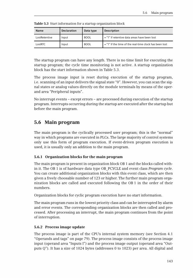
5.6 Main program
143
The startup program can have any length. There is no time limit for executing thestartup program; the cycle time monitoring is not active. A startup organizationblock has the start information shown in Table 5.3.
The process image input is reset during execution of the startup program,i.e. scanning of an input delivers the signal state “0”. However, you can scan the sig-nal states or analog values directly on the module terminals by means of the oper-and area “Peripheral inputs”.
No interrupt events – except errors – are processed during execution of the startupprogram. Interrupts occurring during the startup are executed after the startup butbefore the main program.
5.6 Main program
The main program is the cyclically processed user program; this is the “normal”way in which programs are executed in PLCs. The large majority of control systemsonly use this form of program execution. If event-driven program execution isused, it is usually only an addition to the main program.
5.6.1 Organization blocks for the main program
The main program is present in organization block OB 1 and the blocks called with-in it. The OB 1 is of hardware data type OB_PCYCLE and event class Program cycle.You can create additional organization blocks with this event class, which are thengiven a freely choosable number of 123 or higher. The further main program orga-nization blocks are called and executed following the OB 1 in the order of theirnumbers.
Organization blocks for cyclic program execution have no start information.
The main program runs in the lowest priority class and can be interrupted by alarmand error events. The corresponding organization blocks are then called and pro-cessed. After processing an interrupt, the main program continues from the pointof interruption.
5.6.2 Process image update
The process image is part of the CPU's internal system memory (see Section 4.1“Operands and tags” on page 79). The process image consists of the process imageinput (operand area “Inputs I”) and the process image output (operand area “Out-puts Q”). It has a size of 1024 bytes (addresses 0 to 1023) per area. All digital and
Table 5.3 Start information for a startup organization block
Name Declaration Data type Description
LostRetentive Input BOOL = “1” if retentive data areas have been lost
LostRTC Input BOOL = “1” if the time of the real-time clock has been lost
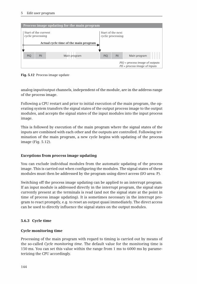
5 Edit user program
144
analog input/output channels, independent of the module, are in the address rangeof the process image.
Following a CPU restart and prior to initial execution of the main program, the op-erating system transfers the signal states of the output process image to the outputmodules, and accepts the signal states of the input modules into the input processimage.
This is followed by execution of the main program where the signal states of theinputs are combined with each other and the outputs are controlled. Following ter-mination of the main program, a new cycle begins with updating of the processimage (Fig. 5.12).
Exceptions from process image updating
You can exclude individual modules from the automatic updating of the processimage. This is carried out when configuring the modules. The signal states of thesemodules must then be addressed by the program using direct access (I/O area: P).
Switching off the process image updating can be applied to an interrupt program.If an input module is addressed directly in the interrupt program, the signal statecurrently present at the terminals is read (and not the signal state at the point intime of process image updating). It is sometimes necessary in the interrupt pro-gram to react promptly, e.g. to reset an output quasi immediately. The direct accesscan be used to directly influence the signal states on the output modules.
5.6.3 Cycle time
Cycle monitoring time
Processing of the main program with regard to timing is carried out by means ofthe so-called Cycle monitoring time. The default value for the monitoring time is150 ms. You can set this value within the range from 1 ms to 6000 ms by parame-terizing the CPU accordingly.
Fig. 5.12 Process image update
PII PIQ PIIPIQ
Start of the current cyclic processing
Start of the next cyclic processing
Actual cycle time of the main program
PIQ = process image of outputsPII = process image of inputs
Main programMain program
Process image updating for the main program
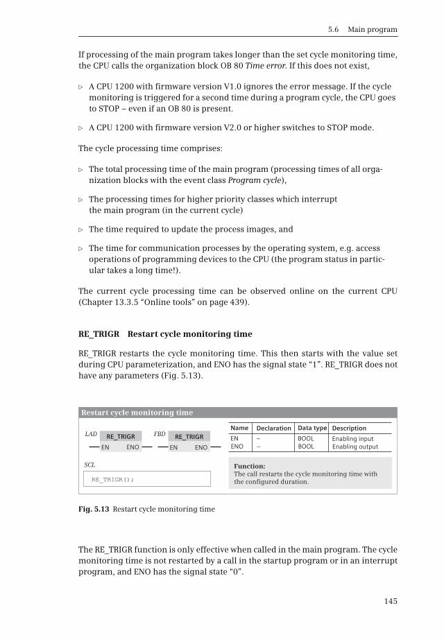
5.6 Main program
145
If processing of the main program takes longer than the set cycle monitoring time,the CPU calls the organization block OB 80 Time error. If this does not exist,
b A CPU 1200 with firmware version V1.0 ignores the error message. If the cycle monitoring is triggered for a second time during a program cycle, the CPU goes to STOP – even if an OB 80 is present.
b A CPU 1200 with firmware version V2.0 or higher switches to STOP mode.
The cycle processing time comprises:
b The total processing time of the main program (processing times of all orga-nization blocks with the event class Program cycle),
b The processing times for higher priority classes which interrupt the main program (in the current cycle)
b The time required to update the process images, and
b The time for communication processes by the operating system, e.g. access operations of programming devices to the CPU (the program status in partic-ular takes a long time!).
The current cycle processing time can be observed online on the current CPU(Chapter 13.3.5 “Online tools” on page 439).
RE_TRIGR Restart cycle monitoring time
RE_TRIGR restarts the cycle monitoring time. This then starts with the value setduring CPU parameterization, and ENO has the signal state “1”. RE_TRIGR does nothave any parameters (Fig. 5.13).
The RE_TRIGR function is only effective when called in the main program. The cyclemonitoring time is not restarted by a call in the startup program or in an interruptprogram, and ENO has the signal state “0”.
Fig. 5.13 Restart cycle monitoring time
Function:
Restart cycle monitoring time
DeclarationName
ENENO
––
BOOLBOOL
Enabling inputEnabling output
DescriptionData typeRE_TRIGR RE_TRIGR
EN ENENO ENO
LAD
SCL
FBD
RE_TRIGR();The call restarts the cycle monitoring time with the configured duration.
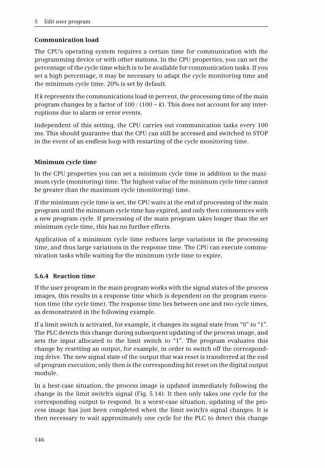
5 Edit user program
146
Communication load
The CPU's operating system requires a certain time for communication with theprogramming device or with other stations. In the CPU properties, you can set thepercentage of the cycle time which is to be available for communication tasks. If youset a high percentage, it may be necessary to adapt the cycle monitoring time andthe minimum cycle time. 20% is set by default.
If k represents the communications load in percent, the processing time of the mainprogram changes by a factor of 100 (100 – k). This does not account for any inter-ruptions due to alarm or error events.
Independent of this setting, the CPU carries out communication tasks every 100ms. This should guarantee that the CPU can still be accessed and switched to STOPin the event of an endless loop with restarting of the cycle monitoring time.
Minimum cycle time
In the CPU properties you can set a minimum cycle time in addition to the maxi-mum cycle (monitoring) time. The highest value of the minimum cycle time cannotbe greater than the maximum cycle (monitoring) time.
If the minimum cycle time is set, the CPU waits at the end of processing of the mainprogram until the minimum cycle time has expired, and only then commences witha new program cycle. If processing of the main program takes longer than the setminimum cycle time, this has no further effects.
Application of a minimum cycle time reduces large variations in the processingtime, and thus large variations in the response time. The CPU can execute commu-nication tasks while waiting for the minimum cycle time to expire.
5.6.4 Reaction time
If the user program in the main program works with the signal states of the processimages, this results in a response time which is dependent on the program execu-tion time (the cycle time). The response time lies between one and two cycle times,as demonstrated in the following example.
If a limit switch is activated, for example, it changes its signal state from “0” to “1”.The PLC detects this change during subsequent updating of the process image, andsets the input allocated to the limit switch to “1”. The program evaluates thischange by resetting an output, for example, in order to switch off the correspond-ing drive. The new signal state of the output that was reset is transferred at the endof program execution; only then is the corresponding bit reset on the digital outputmodule.
In a best-case situation, the process image is updated immediately following thechange in the limit switch's signal (Fig. 5.14). It then only takes one cycle for thecorresponding output to respond. In a worst-case situation, updating of the pro-cess image has just been completed when the limit switch's signal changes. It isthen necessary to wait approximately one cycle for the PLC to detect this change
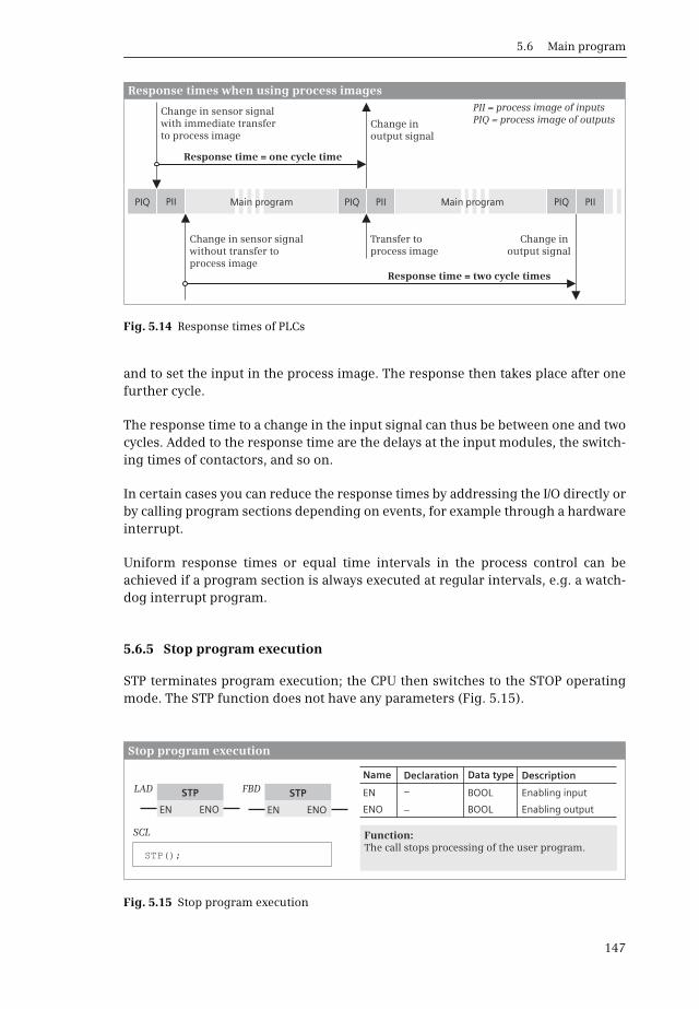
5.6 Main program
147
and to set the input in the process image. The response then takes place after onefurther cycle.
The response time to a change in the input signal can thus be between one and twocycles. Added to the response time are the delays at the input modules, the switch-ing times of contactors, and so on.
In certain cases you can reduce the response times by addressing the I/O directly orby calling program sections depending on events, for example through a hardwareinterrupt.
Uniform response times or equal time intervals in the process control can beachieved if a program section is always executed at regular intervals, e.g. a watch-dog interrupt program.
5.6.5 Stop program execution
STP terminates program execution; the CPU then switches to the STOP operatingmode. The STP function does not have any parameters (Fig. 5.15).
Fig. 5.14 Response times of PLCs
Fig. 5.15 Stop program execution
PII
PII = process image of inputsPIQ = process image of outputs
PII PIIPIQPIQ PIQ
Change in sensor signal with immediate transfer to process image
Change in sensor signal without transfer to process image
Transfer to process image
Change in output signal
Response time = one cycle time
Response times when using process images
Response time = two cycle times
Change in output signal
Main program Main program
Function:
Stop program execution
DeclarationName
EN
ENO
–
–
BOOL
BOOL
Enabling input
Enabling output
DescriptionData type
STP STP
EN ENENO ENO
LAD FBD
SCL
STP();The call stops processing of the user program.
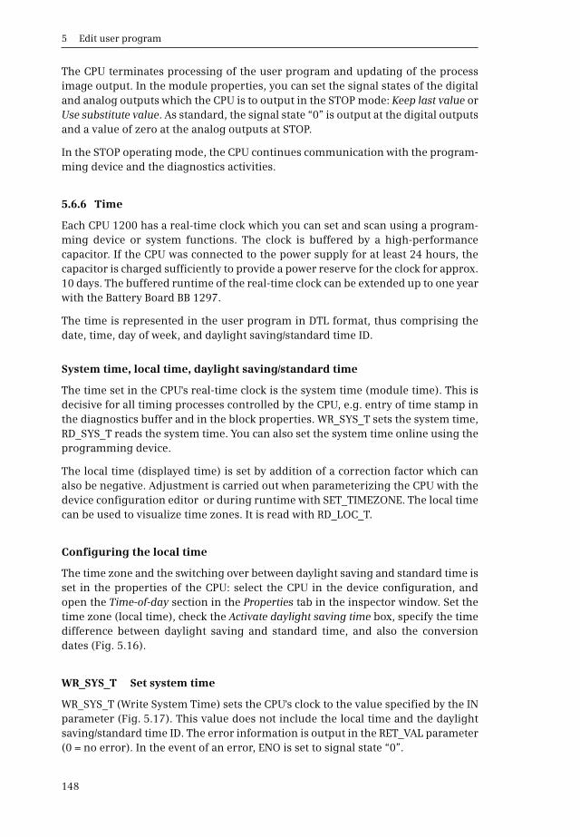
5 Edit user program
148
The CPU terminates processing of the user program and updating of the processimage output. In the module properties, you can set the signal states of the digitaland analog outputs which the CPU is to output in the STOP mode: Keep last value orUse substitute value. As standard, the signal state “0” is output at the digital outputsand a value of zero at the analog outputs at STOP.
In the STOP operating mode, the CPU continues communication with the program-ming device and the diagnostics activities.
5.6.6 Time
Each CPU 1200 has a real-time clock which you can set and scan using a program-ming device or system functions. The clock is buffered by a high-performancecapacitor. If the CPU was connected to the power supply for at least 24 hours, thecapacitor is charged sufficiently to provide a power reserve for the clock for approx.10 days. The buffered runtime of the real-time clock can be extended up to one yearwith the Battery Board BB 1297.
The time is represented in the user program in DTL format, thus comprising thedate, time, day of week, and daylight saving/standard time ID.
System time, local time, daylight saving/standard time
The time set in the CPU's real-time clock is the system time (module time). This isdecisive for all timing processes controlled by the CPU, e.g. entry of time stamp inthe diagnostics buffer and in the block properties. WR_SYS_T sets the system time,RD_SYS_T reads the system time. You can also set the system time online using theprogramming device.
The local time (displayed time) is set by addition of a correction factor which canalso be negative. Adjustment is carried out when parameterizing the CPU with thedevice configuration editor or during runtime with SET_TIMEZONE. The local timecan be used to visualize time zones. It is read with RD_LOC_T.
Configuring the local time
The time zone and the switching over between daylight saving and standard time isset in the properties of the CPU: select the CPU in the device configuration, andopen the Time-of-day section in the Properties tab in the inspector window. Set thetime zone (local time), check the Activate daylight saving time box, specify the timedifference between daylight saving and standard time, and also the conversiondates (Fig. 5.16).
WR_SYS_T Set system time
WR_SYS_T (Write System Time) sets the CPU's clock to the value specified by the INparameter (Fig. 5.17). This value does not include the local time and the daylightsaving/standard time ID. The error information is output in the RET_VAL parameter(0 = no error). In the event of an error, ENO is set to signal state “0”.
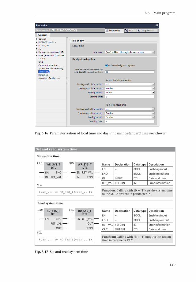
5.6 Main program
149
Fig. 5.16 Parameterization of local time and daylight saving/standard time switchover
Fig. 5.17 Set and read system time
WR_SYS_TDTL
RD_SYS_TDTL
WR_SYS_TDTL
RD_SYS_TDTL
EN
EN
EN
EN
RET_VAL
RET_VAL
OUT
RET_VAL
RET_VAL
ENO
ENO
ENO
OUT
ENO
LAD
LAD
FBD
FBD
IN IN
Declaration
Declaration
Name
Name
EN
EN
ENO
ENO
IN
RET_VAL
RET_VAL
OUT
–
–
–
–
INPUT
RETURN
RETURN
OUTPUT
BOOL
BOOL
BOOL
BOOL
DTL
INT
INT
DTL
Enabling input
Enabling input
Enabling output
Enabling output
Date and time
Error information
Error information
Date and time
Description
Description
Data type
Data type
SCL
SCL
#var_... := WR_SYS_T(#var_...);
#var_... := RD_SYS_T(#var_...);
Read system time
Set system time
Set and read system time
Function: Calling with EN = “1” sets the system time to the value present in parameter IN.
Function: Calling with EN = “1” outputs the system time in parameter OUT.
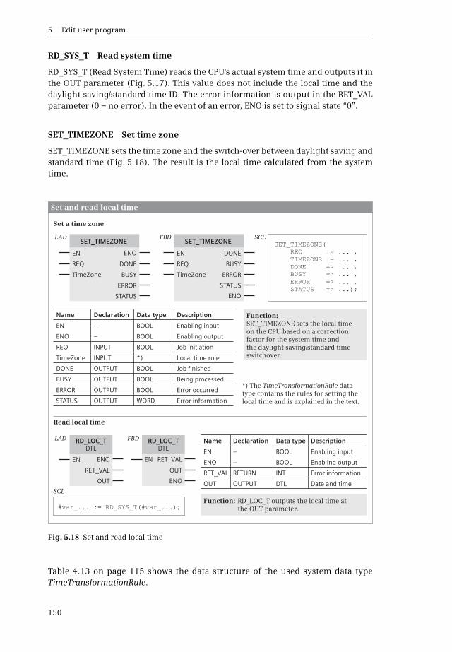
5 Edit user program
150
RD_SYS_T Read system time
RD_SYS_T (Read System Time) reads the CPU's actual system time and outputs it inthe OUT parameter (Fig. 5.17). This value does not include the local time and thedaylight saving/standard time ID. The error information is output in the RET_VALparameter (0 = no error). In the event of an error, ENO is set to signal state “0”.
SET_TIMEZONE Set time zone
SET_TIMEZONE sets the time zone and the switch-over between daylight saving andstandard time (Fig. 5.18). The result is the local time calculated from the systemtime.
Table 4.13 on page 115 shows the data structure of the used system data typeTimeTransformationRule.
Fig. 5.18 Set and read local time
RD_LOC_TDTL
SET_TIMEZONE SET_TIMEZONE
RD_LOC_TDTL
EN
EN EN
REQ REQ
TimeZone TimeZone
EN
RET_VAL
DONE
DONE
OUT
BUSY
BUSY
ERROR
ERROR
STATUS
STATUS
RET_VALENO
ENO
ENO
OUT
ENO
LAD
LAD
FBD
FBD
Set and read local time
Declaration
Declaration
Name
Name
EN
EN
ENO
ENO
RET_VAL
REQ
OUT
TimeZone
DONE
BUSY
ERROR
STATUS
–
–
–
–
RETURN
INPUT
OUTPUT
INPUT
OUTPUT
OUTPUT
OUTPUT
OUTPUT
BOOL
BOOL
BOOL
BOOL
INT
BOOL
DTL
*)
BOOL
BOOL
BOOL
WORD
Enabling input
Enabling input
Enabling output
Enabling output
Error information
Job initiation
Date and time
Local time rule
Job finished
Being processed
Error occurred
Error information
Description
Description
Data type
Data type
Function:
Function:
SCL
SCL
#var_... := RD_SYS_T(#var_...);
SET_TIMEZONE(REQ := ... ,TIMEZONE := ... ,DONE => ... ,BUSY => ... ,ERROR => ... ,STATUS => ...);
Set a time zone
SET_TIMEZONE sets the local time on the CPU based on a correction factor for the system time and the daylight saving/standard time switchover.
*) The TimeTransformationRule data type contains the rules for setting the local time and is explained in the text.
RD_LOC_T outputs the local time at the OUT parameter.
Read local time

5.6 Main program
151
RD_LOC_T Read local time
RD_LOC_T (Read Local Time) reads the CPU's current local time and outputs it in theOUT parameter (Fig. 5.18). The local time is calculated from the system time, thelocal time zone, and the daylight saving/standard time ID. The local time zone andthe daylight saving/standard time ID are set in the properties of the CPU in thedevice configuration editor. The error information is output in the RET_VAL param-eter (0 = no error). In the event of an error, ENO is set to signal state “0”.
Calculating with date and time
You can link the date and time together using further system functions, for exam-ple to generate the difference between two times of day or to add a duration to aspecific point in time. The system functions available are described in the Chapter11.4 “Arithmetic functions for time values” on page 369.
Setting the time on the CPU module online
You can read and set the system time (module time) on the CPU online using theprogramming device. To do this, open the project and start the Online & diagnosticseditor under the PLC station in the project tree. To establish the online mode, clickin the toolbar of the Project view on the Go online symbol or on the Go online buttonin the Online access section of the diagnostics window.
Select the Set time of day command in the Functions section of the diagnostics win-dow. The current time of the programming device is then displayed. For the moduletime (system time on the CPU), you can either select the programming device time,or you can set a separate system time on the CPU module.
Time synchronization
The CPU module time can be synchronized over Ethernet. A time server is requiredwhich synchronizes the time of further stations in the network using the NTP pro-cedure.
Activate the time synchronization in the properties of the PROFINET interface usingthe hardware configuration. To do this, select the PROFINET interface in the deviceconfiguration, and select the Time synchronization command in the properties inthe Inspector window. Check the Enable time-of-day synchronization using NTPmode box, enter the IP addresses of the servers involved, and select the updating in-terval.
5.6.7 Runtime meter
An runtime meter counts the hours while running. You can use the runtime meter,for example, to record the CPU runtime or to determine the operating hours of con-nected devices.
A CPU 1200 has 10 runtime meters with a value range of 32 bits (231–1 hours). Anruntime meter also stops when the CPU is at STOP; if the CPU restarts, the runtime
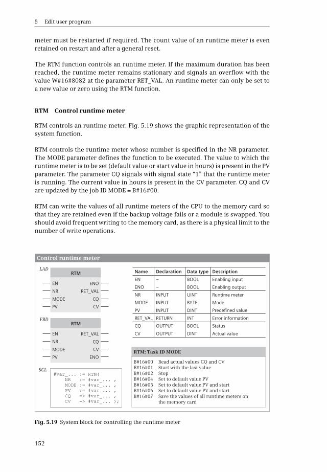
5 Edit user program
152
meter must be restarted if required. The count value of an runtime meter is evenretained on restart and after a general reset.
The RTM function controls an runtime meter. If the maximum duration has beenreached, the runtime meter remains stationary and signals an overflow with thevalue W#16#8082 at the parameter RET_VAL. An runtime meter can only be set toa new value or zero using the RTM function.
RTM Control runtime meter
RTM controls an runtime meter. Fig. 5.19 shows the graphic representation of thesystem function.
RTM controls the runtime meter whose number is specified in the NR parameter.The MODE parameter defines the function to be executed. The value to which theruntime meter is to be set (default value or start value in hours) is present in the PVparameter. The parameter CQ signals with signal state “1” that the runtime meteris running. The current value in hours is present in the CV parameter. CQ and CVare updated by the job ID MODE = B#16#00.
RTM can write the values of all runtime meters of the CPU to the memory card sothat they are retained even if the backup voltage fails or a module is swapped. Youshould avoid frequent writing to the memory card, as there is a physical limit to thenumber of write operations.
Fig. 5.19 System block for controlling the runtime meter
RTM
RTM
Control runtime meter
NR
NR
EN
EN
MODE
MODE
PV
PV
RET_VAL
RET_VAL
ENO
ENO
CV
CV
CQ
CQ
B#16#00 Read actual values CQ and CVB#16#01 Start with the last valueB#16#02 StopB#16#04 Set to default value PVB#16#05 Set to default value PV and startB#16#06 Set to default value PV and startB#16#07
RTM: Task ID MODE
LAD
FBD
DeclarationName
EN
ENO
NR
PV
CQ
MODE
RET_VAL
CV
–
–
INPUT
INPUT
OUTPUT
INPUT
RETURN
OUTPUT
BOOL
BOOL
UINT
DINT
BOOL
BYTE
INT
DINT
Enabling input
Enabling output
Predefined value
Status
Mode
Error information
Actual value
DescriptionData type
SCL#var_... := RTM(
NR := #var_... ,MODE := ... ,PV := ... ,CQ => ... ,CV => ... );
#var_#var_#var_#var_
Runtime meter
Save the values of all runtime meters on the memory card
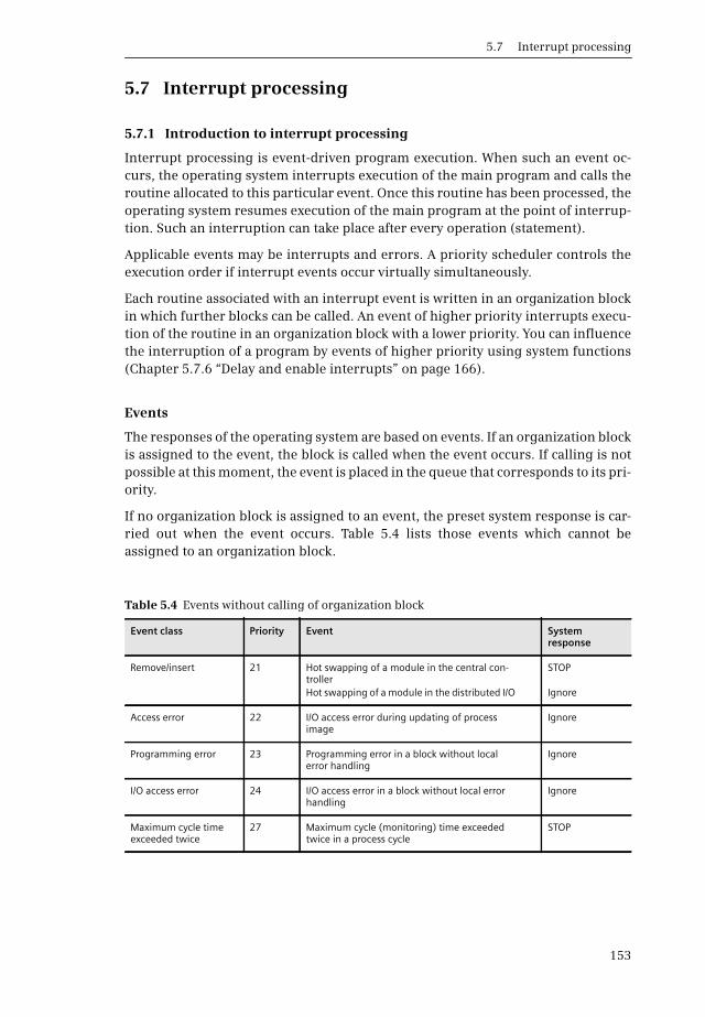
5.7 Interrupt processing
153
5.7 Interrupt processing
5.7.1 Introduction to interrupt processing
Interrupt processing is event-driven program execution. When such an event oc-curs, the operating system interrupts execution of the main program and calls theroutine allocated to this particular event. Once this routine has been processed, theoperating system resumes execution of the main program at the point of interrup-tion. Such an interruption can take place after every operation (statement).
Applicable events may be interrupts and errors. A priority scheduler controls theexecution order if interrupt events occur virtually simultaneously.
Each routine associated with an interrupt event is written in an organization blockin which further blocks can be called. An event of higher priority interrupts execu-tion of the routine in an organization block with a lower priority. You can influencethe interruption of a program by events of higher priority using system functions(Chapter 5.7.6 “Delay and enable interrupts” on page 166).
Events
The responses of the operating system are based on events. If an organization blockis assigned to the event, the block is called when the event occurs. If calling is notpossible at this moment, the event is placed in the queue that corresponds to its pri-ority.
If no organization block is assigned to an event, the preset system response is car-ried out when the event occurs. Table 5.4 lists those events which cannot beassigned to an organization block.
Table 5.4 Events without calling of organization block
Event class Priority Event System response
Remove/insert 21 Hot swapping of a module in the central con-trollerHot swapping of a module in the distributed I/O
STOP
Ignore
Access error 22 I/O access error during updating of process image
Ignore
Programming error 23 Programming error in a block without local error handling
Ignore
I/O access error 24 I/O access error in a block without local error handling
Ignore
Maximum cycle time exceeded twice
27 Maximum cycle (monitoring) time exceeded twice in a process cycle
STOP
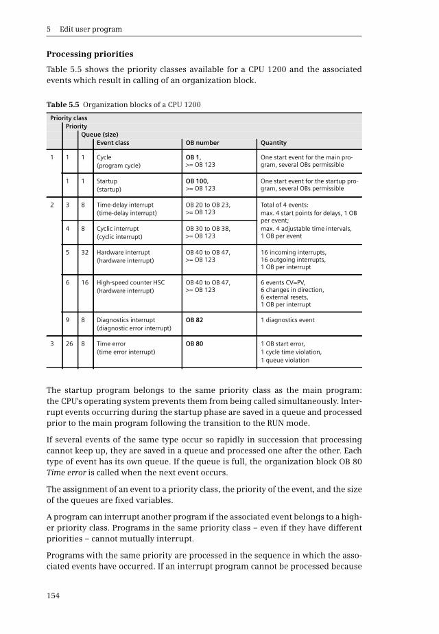
5 Edit user program
154
Processing priorities
Table 5.5 shows the priority classes available for a CPU 1200 and the associatedevents which result in calling of an organization block.
The startup program belongs to the same priority class as the main program:the CPU's operating system prevents them from being called simultaneously. Inter-rupt events occurring during the startup phase are saved in a queue and processedprior to the main program following the transition to the RUN mode.
If several events of the same type occur so rapidly in succession that processingcannot keep up, they are saved in a queue and processed one after the other. Eachtype of event has its own queue. If the queue is full, the organization block OB 80Time error is called when the next event occurs.
The assignment of an event to a priority class, the priority of the event, and the sizeof the queues are fixed variables.
A program can interrupt another program if the associated event belongs to a high-er priority class. Programs in the same priority class – even if they have differentpriorities – cannot mutually interrupt.
Programs with the same priority are processed in the sequence in which the asso-ciated events have occurred. If an interrupt program cannot be processed because
Table 5.5 Organization blocks of a CPU 1200
Priority classPriority
Queue (size)Event class OB number Quantity
1 1 1 Cycle(program cycle)
OB 1, >= OB 123
One start event for the main pro-gram, several OBs permissible
1 1 Startup(startup)
OB 100, >= OB 123
One start event for the startup pro-gram, several OBs permissible
2 3 8 Time-delay interrupt(time-delay interrupt)
OB 20 to OB 23, >= OB 123
Total of 4 events:max. 4 start points for delays, 1 OB per event;max. 4 adjustable time intervals, 1 OB per event
4 8 Cyclic interrupt(cyclic interrupt)
OB 30 to OB 38, >= OB 123
5 32 Hardware interrupt(hardware interrupt)
OB 40 to OB 47, >= OB 123
16 incoming interrupts, 16 outgoing interrupts, 1 OB per interrupt
6 16 High-speed counter HSC(hardware interrupt)
OB 40 to OB 47, >= OB 123
6 events CV=PV,6 changes in direction,6 external resets,1 OB per interrupt
9 8 Diagnostics interrupt (diagnostic error interrupt)
OB 82 1 diagnostics event
3 26 8 Time error(time error interrupt)
OB 80 1 OB start error, 1 cycle time violation,1 queue violation
5.7 Interrupt processing
155
a program of higher priority is currently being processed, the event is entered intothe queue. The associated program is then processed when the program of higherpriority has been completed, and if no other event of higher priority is present.
The main program has the lowest processing priority. Only one interrupt organiza-tion block can be processed at a time, which can then be interrupted by the organi-zation block OB 80 Time error.
Types of interrupt
The CPU 1200 provides the following interrupt events (interrupts):
b Time-delay interruptAn interrupt generated when a certain period of time has passed; a system function defines the time at which this period begins
b Cyclic interruptAn interrupt generated by the operating system at periodic intervals
b Hardware interruptAn interrupt from a module, either via an input derived from a process signal or generated on the module itself (e.g. by a high-speed counter HSC).
Other interrupt events are the time error (Section 5.8.3 “Time error OB 80” onpage 168) and the diagnostics interrupt (Section 5.8.6 “Diagnostics interrupt OB 82”on page 176).
Current signal states
In an interrupt routine it is sometimes necessary to work with the current signalstates of the I/O modules and not with the signal states of the inputs that were up-dated at the start of the main program. The fetched signal states are then writtendirectly to the I/O without waiting until the output process image has been updatedat the end of the main program.
The operand area I/O permits direct access to the signal states on the module termi-nals (Section 4.1 “Operands and tags” on page 79). Note that the signal states on themodule terminals change asynchronous to the cyclic program execution. It is there-fore recommendable to maintain a strict separation between the main programand the interrupt routine.
5.7.2 Time-delay interrupts
A time-delay interrupt implements a delay time independent of the timer functionsand asynchronous to cyclic program execution. With a CPU 1200, the organizationblocks OB 20 to OB 23 and OB 123 and higher are set aside for processing a time-delay interrupt.
Such an organization block is assigned to event class Time-delay interrupt. It is ofhardware data type OB_Delay. The System constants tab of the default tag table liststhe names and values of the constants. The name of the constant can be changed inthe block properties.

5 Edit user program
156
Using a time-delay interrupt
A time-delay interrupt is started by calling the system function SRT_DINT; thissystem function also passes on the delay interval and the delay organizationblock. When the delay interval has expired, the corresponding organization blockis called.
The time between calling SRT_DINT and starting the organization block is a maxi-mum of one millisecond less than the configured delay time providing that nointerrupt events delay the call.
You can also use the CAN_DINT function to cancel execution of a time-delay inter-rupt that has not yet started. The associated organization block is then no longercalled.
Calling of a time-delay interrupt OB can be delayed or enabled using the DIS_AIRTand EN_AIRT functions.
You must not use more than a total of four time-delay interrupt and cyclic interruptorganization blocks in your program.
Time-delay interrupt organization blocks do not have any startup information.
Behavior during startup
During a startup, the operating system deletes all settings you have programmedfor time-delay interrupts.
You can start a time-delay interrupt in the startup program by calling SRT_DINT.Following expiry of the delay time, the CPU must be in the RUN operating mode inorder to process the corresponding organization block. If this is not the case, theCPU waits with the OB call until the startup has been completed and then calls thetime-delay interrupt OB before the first statement in the main program.
Configuring time-delay interrupts
Configuration of the time-delay interrupts is carried out in two steps:
b First create a user organization block for a time-delay interrupt.
b Then program the SRT_DINT function and possibly the CAN_DINT and QRY_DINT functions and assign the number of the time-delay interrupt OB to the OB_NR parameter.
To create an organization block for a time-delay interrupt, open the project in theProject view. In the project tree, double-click on Add new block under Programblocks. Click on Organization block (OB) in the Add new block window, and then onthe start event Time delay interrupt. Assign a meaningful name to the OB, define theprogramming language, and select Manual if the OB is to have a number different
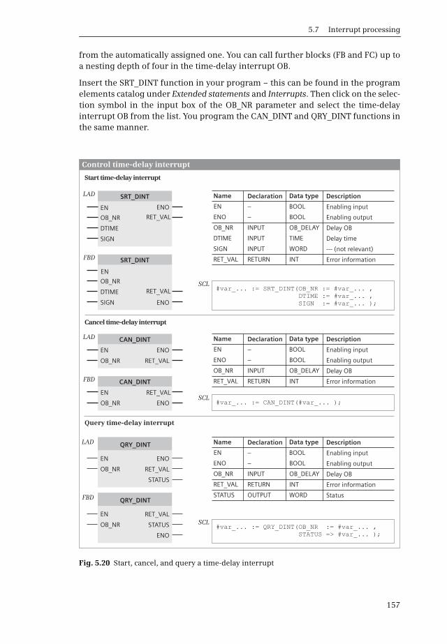
5.7 Interrupt processing
157
from the automatically assigned one. You can call further blocks (FB and FC) up toa nesting depth of four in the time-delay interrupt OB.
Insert the SRT_DINT function in your program – this can be found in the programelements catalog under Extended statements and Interrupts. Then click on the selec-tion symbol in the input box of the OB_NR parameter and select the time-delayinterrupt OB from the list. You program the CAN_DINT and QRY_DINT functions inthe same manner.
Fig. 5.20 Start, cancel, and query a time-delay interrupt
Declaration
Declaration
Declaration
Name
Name
Name
EN
EN
EN
ENO
ENO
ENO
OB_NR
OB_NR
OB_NR
DTIME
SIGN
RET_VAL
RET_VAL
RET_VAL
STATUS
–
–
–
–
–
–
INPUT
INPUT
INPUT
INPUT
INPUT
RETURN
RETURN
RETURN
OUTPUT
BOOL
BOOL
BOOL
BOOL
BOOL
BOOL
OB_DELAY
OB_DELAY
OB_DELAY
TIME
WORD
INT
INT
INT
WORD
Enabling input
Enabling input
Enabling input
Enabling output
Enabling output
Enabling output
Delay OB
Delay OB
Delay OB
Delay time
--- (not relevant)
Error information
Error information
Error information
Status
Description
Description
Description
Data type
Data type
Data type
Control time-delay interrupt
SRT_DINT
CAN_DINT
SRT_DINT
CAN_DINT
EN
EN
EN
EN
ENO
ENO
ENO
ENO
LAD
LAD
FBD
FBD
RET_VAL
RET_VAL
RET_VAL
RET_VAL
OB_NR
OB_NR
OB_NR
OB_NR
DTIME
DTIME
SIGN
SIGN
QRY_DINT
QRY_DINT
Start time-delay interrupt
Cancel time-delay interrupt
Query time-delay interrupt
EN
EN
OB_NR
OB_NR
ENO
RET_VAL
RET_VAL
STATUS
STATUS
ENO
LAD
FBD
SCL
SCL
SCL
#var_... := SRT_DINT(OB_NR := #var_... ,DTIME := #var_... ,SIGN := #var_... );
#var_... := CAN_DINT(#var_... );
#var_... := QRY_DINT(OB_NR := #var_... ,STATUS => #var_... );
5 Edit user program
158
System functions for editing a time-delay interrupt
You can control a time-delay interrupt using the following functions:
b SRT_DINT Start time-delay interrupt
b CAN_DINT Cancel time-delay interrupt
b QRY_DINT Querying the status of a time-delay interrupt
Calling of these functions is shown in Fig. 5.20. You can also connect a constant ora tag of data type WORD or INT to the OB_NR parameter if the IEC check attribute isnot activated.
SRT_DINT Start time-delay interrupt
SRT_DINT starts a time-delay interrupt. The function call is simultaneously the starttime for the parameterized period. Once the delay time has expired, the CPU callsthe parameterized OB. You can set the delay time in intervals of 1 ms. The accuracyof the delay time is also 1 ms.
The SIGN parameter has no significance with a CPU 1200, but it must neverthelessbe supplied. You can assign it a constant value of zero (0), for example.
Note that processing of a time-delay interrupt OB may be delayed if organizationblocks of higher priority are being processed when the OB is called. The call is alsodelayed by use of the DIS_AINT function.
You can overwrite a current delay time by a new value by calling SRT_DINT again.The new delay time then commences when the function is called.
CAN_DINT Cancel time-delay interrupt
CAN_DINT cancels a started time-delay interrupt. The organization block selectedby the OB_NR parameter is not called in this case.
QRY_DINT Querying the status of a time-delay interrupt
QRY_DINT queries the status of a time-delay interrupt. The time-delay interrupt isspecified with the parameter OB_NR. The STATUS parameter contains the desiredinformation and the individual bits have the significance shown in Table 5.6.
Error response
If the time-delay interrupt OB is not present in the user program when called, theoperating system signals a program execution error which can be processed usingthe GET_ERR_ID and GET_ERROR functions.
If the delay time has expired and the associated OB is still being processed, the oper-ating system calls OB 80 Time error. The error is ignored if OB 80 is not present.
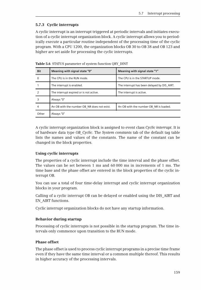
5.7 Interrupt processing
159
5.7.3 Cyclic interrupts
A cyclic interrupt is an interrupt triggered at periodic intervals and initiates execu-tion of a cyclic interrupt organization block. A cyclic interrupt allows you to period-ically execute a particular routine independent of the processing time of the cyclicprogram. With a CPU 1200, the organization blocks OB 30 to OB 38 and OB 123 andhigher are set aside for processing the cyclic interrupts.
A cyclic interrupt organization block is assigned to event class Cyclic interrupt. It isof hardware data type OB_Cyclic. The System constants tab of the default tag tablelists the names and values of the constants. The name of the constant can bechanged in the block properties.
Using cyclic interrupts
The properties of a cyclic interrupt include the time interval and the phase offset.The values can be set between 1 ms and 60 000 ms in increments of 1 ms. Thetime base and the phase offset are entered in the block properties of the cyclic in-terrupt OB.
You can use a total of four time-delay interrupt and cyclic interrupt organizationblocks in your program.
Calling of a cyclic interrupt OB can be delayed or enabled using the DIS_AIRT andEN_AIRT functions.
Cyclic interrupt organization blocks do not have any startup information.
Behavior during startup
Processing of cyclic interrupts is not possible in the startup program. The time in-tervals only commence upon transition to the RUN mode.
Phase offset
The phase offset is used to process cyclic interrupt programs in a precise time frameeven if they have the same time interval or a common multiple thereof. This resultsin higher accuracy of the processing intervals.
Table 5.6 STATUS parameter of system function QRY_DINT
Bit Meaning with signal state “0” Meaning with signal state “1”
0 The CPU is in the RUN mode. The CPU is in the STARTUP mode.
1 The interrupt is enabled. The interrupt has been delayed by DIS_AIRT.
2 The interrupt expired or is not active. The interrupt is active.
3 Always “0”
4 An OB with the number OB_NR does not exist. An OB with the number OB_NR is loaded.
Other Always “0”
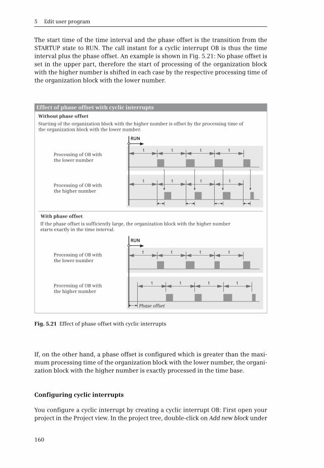
5 Edit user program
160
The start time of the time interval and the phase offset is the transition from theSTARTUP state to RUN. The call instant for a cyclic interrupt OB is thus the timeinterval plus the phase offset. An example is shown in Fig. 5.21: No phase offset isset in the upper part, therefore the start of processing of the organization blockwith the higher number is shifted in each case by the respective processing time ofthe organization block with the lower number.
If, on the other hand, a phase offset is configured which is greater than the maxi-mum processing time of the organization block with the lower number, the organi-zation block with the higher number is exactly processed in the time base.
Configuring cyclic interrupts
You configure a cyclic interrupt by creating a cyclic interrupt OB: First open yourproject in the Project view. In the project tree, double-click on Add new block under
Fig. 5.21 Effect of phase offset with cyclic interrupts
t
t tt t
t
t
t
t
t
t
t
tt t t
Phase offset
RUN
RUN
Without phase offset
With phase offset
Effect of phase offset with cyclic interrupts
Starting of the organization block with the higher number is offset by the processing time of the organization block with the lower number.
If the phase offset is sufficiently large, the organization block with the higher number starts exactly in the time interval.
Processing of OB with the lower number
Processing of OB with the higher number
Processing of OB with the lower number
Processing of OB with the higher number

5.7 Interrupt processing
161
Program blocks. Click on Organization block (OB) in the Add new block window, andthen on Cyclic interrupt.
Assign a meaningful name to the OB, define the programming language, and selectManual if the OB is to have a number different from the automatically assigned one.
You can call further blocks (FB and FC) up to a nesting depth of four in the cyclicinterrupt OB.
The time base and the phase offset are entered in the block properties. With thecyclic interrupt OB open, click Cyclic interrupt in the Inspector window underProperties and enter the time base and phase offset in milliseconds.
System functions for editing a cyclic interrupt
You can set and query the parameters for processing a cyclic interrupt with the fol-lowing functions:
b SET_CINT Set cyclic interrupt parameters
b QRY_CINT Query cyclic interrupt parameters
Calling of these functions is shown in Fig. 5.22. You can also connect a constant ora tag of data type WORD or INT to the OB_NR parameter if the IEC check attribute isnot activated.
SET_CINT Set cyclic interrupt parameters
SET_CINT sets the parameters for a cyclic interrupt. These are the interval withwhich the cyclic interrupt is triggered, and the phase offset. Enter the time intervalin microseconds at the CYCLE parameter. If the time interval is zero, the cyclic inter-rupt organization block specified in parameter OB_NR is not called. The phase off-set at parameter PHASE is also specified in microseconds.
QRY_CINT Query cyclic interrupt parameters
QRY_CINT reads the parameters of the cyclic interrupt organization block specifiedat parameter OB_NR and outputs them to the parameters CYCLE (time interval) andPHASE (phase offset). The operating mode of the selected cyclic interrupt organiza-tion block is output at parameter STATUS (Table 5.7).
Error response
If the cyclic interrupt OB is not present in the user program when called, the oper-ating system signals a program execution error which can be processed using theGET_ERR_ID and GET_ERROR functions.
The processing time of a cyclic interrupt organization block must be significantlyshorter than its time frame. If the associated cyclic interrupt is repeated during anongoing cyclic interrupt OB, the operating system calls OB 80 Time error. The erroris ignored if OB 80 is not present.

5 Edit user program
162
Fig. 5.22 Set and query cyclic interrupt parameters
Table 5.7 STATUS parameter of system function QRY_CINT
Bit Meaning with signal state “0” Meaning with signal state “1”
0 The CPU is in the RUN mode. The CPU is in the STARTUP mode.
1 The interrupt is enabled. The interrupt has been delayed by DIS_AIRT.
2 The interrupt expired or is not active. The interrupt is active.
3 Always “0”
4 An OB with the number OB_NR does not exist. An OB with the number OB_NR is loaded.
Other Always “0”
Declaration
Declaration
Name
Name
EN
EN
ENO
ENO
OB_NR
OB_NR
CYCLE
PHASE
RET_VAL
RET_VAL
CYCLE
PHASE
STATUS
–
–
–
–
INPUT
INPUT
INPUT
INPUT
RETURN
RETURN
OUTPUT
OUTPUT
OUTPUT
BOOL
BOOL
BOOL
BOOL
OB_CYCLE
OB_CYCLE
UDINT
UDINT
INT
INT
UDINT
UDINT
WORD
Enabling input
Enabling input
Enabling output
Enabling output
Cyclic-interrupt OB
Delay OB
Time interval (µs)
Phase offset
Error information
Error information
Time interval (µs)
Phase offset
Status
Description
Description
Data type
Data type
Set and query parameters for processing a cyclic interrupt
SET_CINT
SET_CINT
EN
EN
ENO
ENO
LAD
FBD
RET_VAL
RET_VAL
OB_NR
OB_NR
CYCLE
CYCLE
PHASE
PHASE
QRY_DINT
QRY_DINT
EN
EN
OB_NR
OB_NR
ENO
RET_VAL
RET_VAL
CYCLE
PHASE
STATUS
CYCLE
PHASE
STATUS
ENO
LAD
FBD
SCL
SCL
#var_... := SET_CINT(OB_NR := #var_... ,CYCLE := #var_... ,PHASE := #var_... );
#var_... := QRY_CINT(OB_NR := #var_... ,CYCLE => #var_... ,PHASE => #var_... ,STATUS => #var_... );
Set parameters
Query parameters
5.7 Interrupt processing
163
5.7.4 Process interrupts
A hardware interrupt summarizes events in the controlled process or a module andresponds immediately with a corresponding program. With a CPU 1200, the orga-nization blocks OB 40 to OB 47 and OB 123 and higher are set aside for processinga cyclic interrupt.
A hardware interrupt organization block is assigned to event class Hardwareinterrupt. It is of hardware data type OB_HWINT. The System constants tab of the de-fault tag table lists the names and values of the constants. The name of the constantcan be changed in the block properties.
You can use up to 50 independent process interrupt OBs. Only one hardware inter-rupt OB can be assigned to a hardware interrupt event, but several events can be as-signed to one hardware interrupt OB.
Triggering a hardware interrupt
Possible sources of hardware interrupt events are:
b All onboard digital input channels of the CPU module
b Plus the digital input channels on the signal board and
b The signals of a high-speed counter HSC (CV = PV, change in counting direction, and external reset)
Triggering of a hardware interrupt is initially disabled by default. You can enablethe processing of a process interrupt when parameterizing using the device config-uration editor. With the digital input channels you can select whether the hardwareinterrupt is to be triggered by an incoming event, an outgoing event, or by both.
If, during processing of a hardware interrupt OB, an event occurs on the same chan-nel of the same module which would again trigger the freshly processed hardwareinterrupt, this process interrupt is lost. A new hardware interrupt is only detectedwhen processing of the old hardware interrupt has been completed. If the event towhich the same process interrupt OB is assigned occurs on a different channel ofthe same module or on a different module, the operating system starts the organi-zation block again following processing of the process interrupt OB.
Using the hardware interrupt
Hardware interrupt OBs are only called in the RUN mode.
Hardware interrupt organization blocks do not have any startup information.
At runtime, the assignment between a hardware interrupt event and an organiza-tion block can be made or removed.
Calling of a hardware interrupt OB can be delayed or enabled using the DIS_AIRTand EN_AIRT functions.

5 Edit user program
164
Behavior during startup
The modules do not generate hardware interrupt events in STARTUP mode. Inter-rupt handling commences with the transition to the RUN operating mode. Hard-ware interrupts present during the transition are lost.
Activate hardware interrupt event
If an onboard input of the CPU module is to trigger a hardware interrupt, start thedevice configuration editor, select the CPU module, and change in the Inspectorwindow to the Properties tab. In the Digital inputs section, select the associated chan-nel and activate the hardware interrupt.
If a digital input on the signal board is to trigger a hardware interrupt, select thesignal board, and change in the Inspector window to the Properties tab. UnderDigital inputs in the DIx/DOx section, select the associated channel and activate theprocess interrupt.
If a high-speed counter is to trigger a hardware interrupt, select the CPU module,and change in the Inspector window to the Properties tab. Select the associatedcounter in the High-speed counters (HSC) section, activate it under General, and setthe counter function. Under Event configuration, you can activate the hardware in-terrupt.
When activating the hardware interrupt, you can assign a name to the event andcreate the associated process interrupt OB: Open the Hardware interrupt input boxand select the hardware interrupt OB in the window (if it has already been created),or create a new one using Add object.
Hardware interrupt organization block
Open a project in the Project view. In the project tree, double-click on Add new blockunder Program blocks. Select Organization block (OB) and the associated event classHardware interrupt. Assign a meaningful name to the organization block, andchange the programming language and the number of the block if necessary.
Error response
If the hardware interrupt OB is not present in the user program when called, theoperating system signals a program execution error which can be processed usingthe GET_ERR_ID and GET_ERROR functions.
5.7.5 Assigning interrupts during runtime
With the following functions you can assign an organization block to an interruptevent during runtime and cancel the assignment again:
b ATTACH Assign organization block to the interrupt event
b DETACH Remove organization block from the interrupt event
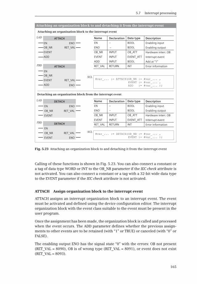
5.7 Interrupt processing
165
Calling of these functions is shown in Fig. 5.23. You can also connect a constant ora tag of data type WORD or INT to the OB_NR parameter if the IEC check attribute isnot activated. You can also connect a constant or a tag with a 32-bit wide data typeto the EVENT parameter if the IEC check attribute is not activated.
ATTACH Assign organization block to the interrupt event
ATTACH assigns an interrupt organization block to an interrupt event. The eventmust be activated and defined using the device configuration editor. The interruptorganization block with the event class suitable to the event must be present in theuser program.
Once the assignment has been made, the organization block is called and processedwhen the event occurs. The ADD parameter defines whether the previous assign-ments to other events are to be retained (with “1” or TRUE) or canceled (with “0” orFALSE).
The enabling output ENO has the signal state “0” with the errors: OB not present(RET_VAL = 8090), OB is of wrong type (RET_VAL = 8091), or event does not exist(RET_VAL = 8093).
Fig. 5.23 Attaching an organization block to and detaching it from the interrupt event
Declaration
Declaration
Name
Name
EN
EN
ENO
ENO
OB_NR
OB_NR
EVENT
ADD
RET_VAL
EVENT
RET_VAL
–
–
–
–
INPUT
INPUT
INPUT
INPUT
RETURN
INPUT
RETURN
BOOL
BOOL
BOOL
BOOL
OB_ATT
OB_ATT
EVENT_ATT
BOOL
INT
EVENT_ATT
INT
Enabling input
Enabling input
Enabling output
Enabling output
Hardware interr. OB
Hardware interr. OB
Interrupt event
Add at “1”
Error information
Interrupt event
Error information
Description
Description
Data type
Data type
Attaching an organization block to and detaching it from the interrupt event
ATTACH
DETACH
ATTACH
DETACH
EN
EN
EN
EN
ENO
ENO
ENO
RET_VAL
ENO
LAD
LAD
FBD
FBD
RET_VAL
RET_VAL
RET_VAL
OB_NR
OB_NR
EVENT
OB_NR
OB_NR
EVENT
EVENT
EVENT
ADD
ADD
SCL
SCL
#var_... := ATTACH(OB_NR := #var_... ,EVENT := #var_... ,ADD := #var_... );
#var_... := DETACH(OB_NR := #var_... ,EVENT := #var_... );
Attaching an organization block to the interrupt event
Detaching an organization block from the interrupt event

5 Edit user program
166
DETACH Remove organization block from the interrupt event
DETACH removes the assignment of an interrupt event to an interrupt organizationblock.
If an event is specified in the EVENT parameter, the assignment of this event is can-celed. If the EVENT parameter is “0”, all assignments to the OB present on parame-ter OB_NR are canceled.
If the requested assignment does not exist, the enabling output ENO has the signalstate “0” and a value of 1 is output in the RET_VAL parameter. Further errors are:OB not present (RET_VAL = 8090), OB is of wrong type (RET_VAL = 8091), or eventdoes not exist (RET_VAL = 8093).
5.7.6 Delay and enable interrupts
The following program functions are available for delaying and enabling inter-rupts:
b DIS_AIRT Delay interrupt events
b EN_AIRT Enable delayed interrupt events
Calling of these functions is shown in Fig. 5.24.
DIS_AIRT Delay interrupt events
Following calling of the DIS_AIRT function, the program in the current organiza-tion block (in the current priority class) is not interrupted by an interrupt event ofhigher priority should this occur. The interrupts are processed with a delay, i.e. the
Fig. 5.24 Delay and enable interrupt events
Delay and enable interrupt events
Declaration
Declaration
Name
Name
EN
EN
ENO
ENO
RET_VAL
RET_VAL
–
–
–
–
RETURN
RETURN
BOOL
BOOL
BOOL
BOOL
INT
INT
Enabling input
Enabling input
Enabling output
Enabling output
Number of calls
Number of calls
Description
Description
Data type
Data type
DIS_AIRT
EN_AIRT
DIS_AIRT
EN_AIRT
EN
EN
EN
EN
ENO
ENO
RET_VAL
RET_VAL
RET_VAL
RET_VAL
ENO
ENO
LAD
LAD
FBD
FBD
SCL
SCL
#var_... := DIS_AIRT();
#var_... := EN_AIRT();
Delay interrupt events
Enable interrupt events

5.8 Troubleshooting, diagnostics
167
operating system saves the interrupt events occurring during the delay and onlyprocesses them when the delay has been canceled. No interrupts are lost.
The delay in processing is retained until the end of processing of the current orga-nization block or until the EN_AIRT function is called.
You can call several DIS_AIRT functions in succession. The RET_VAL parameter indi-cates the (new) number of calls. You must then call EN_AIRT exactly as often asDIS_AIRT so that the processing of all interrupts is enabled again.
EN_AIRT Enable delayed interrupt events
The EN_AIRT function enables processing of the interrupts again which have beendelayed with DIS_AIRT. You must call EN_AIRT exactly as often as you previouslycalled DIS_AIRT in the current organization block or in the blocks called within thisorganization block.
The RET_VAL parameter indicates the (still remaining) number of effective delays.If RET_VAL is equal to 0, processing of all interrupts has been enabled again.
5.8 Troubleshooting, diagnostics
5.8.1 Causes of errors and responses
The CPU can detect and signal errors in the program execution.These errors include:
b Errors in arithmetic operations (overflow, invalid floating-point number)
b Errors when calling blocks (block does not exist or is still being processed,program execution error)
b Errors when addressing the peripheral inputs and outputs (access errors)
In the event of “serious” errors, e.g. cycle monitoring time expired twice in a pro-gram cycle, the CPU directly enters the STOP mode.
Errors which are module-based are signaled by the diagnostics function. This canbe carried out via the ERROR LED on the front of the CPU, via an entry in the diag-nostics buffer, or by starting the diagnostics interrupt (see Chapter 13.3 “Hardwarediagnostics” on page 436).
Error handling in general
The occurrence of an error can be signaled by the following responses:
b The ENO output of a program function is set to “0” if the function has been executed incorrectly or not at all.
b The operating system starts the standard error handling, e.g. with a “fatal” error it enters the STOP mode or calls organization block OB 80 Time error.
b The operating system relinquishes the standard error handling and applies the (block) local error handling instead.

5 Edit user program
168
5.8.2 Error display with the ENO output
System functions for which an error can occur during processing and callable logicblocks (functions, function blocks) have an enable output ENO, with which the errorin the calling program can be reported. An error is present if the ENO output has sig-nal state “0” or is FALSE.
For LAD and FBD, the ENO output is represented as an output parameter at the callbox. For SCL, the ENO output is not represented by default. If you want to use it, addscanning of the ENO output to the last position in the parameter list. You can scanthe ENO output in the calling block and respond to the error (Chapter 12.4 “EN/ENOmechanism” on page 417).
In a self-written block, transfer an error message to the ENO output with a blockend function (Chapter 12.2 “Block end function” on page 412). Examples ofdetected errors in the user program are diagnostics alarms, e.g. wire break at ananalog input, or malfunction of the controlled machine, e.g. the simultaneousassignment of two conflicting limit switches.
5.8.3 Time error OB 80
The operating system calls the organization block OB 80 Time error when one ofthe following events occurs:
b Cycle monitoring time exceeded
b OB request error: the requested organization block is still being processed (possible with time-delay and cyclic interrupts) or an organization block is requested too frequently within a given priority class (queue overflow)
b An interrupt is lost due to interrupt overload.
The time error organization block is assigned to event class Time error interrupt. Itis of hardware data type OB_TIMEERROR. The System constants tab of the default tagtable lists the name and value of the constant. The name of the constant can bechanged in the block properties.
Only one time error organization block can be programmed.
The error is ignored if OB 80 is not present when a time error occurs.
Start information
Table 5.8 shows the start information for OB 80. The tags in the start informationare transferred to the Input section of the block interface and are present in the tem-porary local data.

5.8 Troubleshooting, diagnostics
169
5.8.4 Local error handling
You can program local error handling in organization blocks (OB), functionblocks (FB) and functions (FC). This only applies to the corresponding block. Thelocal error handling is neither accepted by the calling block nor passed on to thecalled block. If the local error handling is not programmed, the system settingsapply when an error occurs (ignore error or STOP).
The default responses are as follows with the local error handling active:
b With a write error: the error is ignored, and program execution is continued.
b With a read error: the substitute value “0” or zero is read, and program executionis continued.
b With an execution error: execution of the faulty statement (function) is aborted,and program execution is continued with the next statement.
Local error handling is automatically activated by inserting the GET_ERROR orGET_ERROR_ID statement in the block, and indicated in the block properties by theHandle errors within block attribute (cannot be edited).
Evaluating program errors
Two functions are available for the evaluation of errors in the case of local errorhandling in the block (Fig. 5.25):
b GET_ERR_ID (read program error number) provides the error number (identifi-cation) when a program execution error occurs.
b GET_ERROR (read program error information) provides the corresponding in-formation in a predefined data structure when a program execution error oc-curs.
In the event of a program execution error, the CPU enters the error into the diag-nostics buffer as standard, and goes to STOP. If the GET_ERROR or GET_ERR_IDfunction is programmed in the block, there is neither an entry into the diagnosticsbuffer nor a change to STOP. Instead of this, the error is signaled by means ofGET_ERROR or GET_ERR_ID.
The error may have occurred at any position between starting of the block andcalling of GET_ERROR or GET_ERR_ID. Therefore, in the case of a single call of
Table 5.8 Start information for OB 80
Variable Data type Description
fault_id BYTE Error IDB#01: Maximum cycle time exceededB#02: Called OB is still executingB#07: Queue overflowB#09: Interrupt loss due to high interrupt load
csg_OBnr OB_ANY Number of OB being processed at time of error
csg_prio UINT Priority of OB being processed at time of error

5 Edit user program
170
GET_ERROR or GET_ERR_ID, the call is preferably positioned in the last network ofthe monitored block.
GET_ERROR and GET_ERR_ID can also be called more than once. Calling of GET_ERROR or GET_ERR_ID reinitiates error recording. The next call of GET_ERROR orGET_ERR_ID outputs the first error following the previous call of GET_ERROR orGET_ERR_ID. The sequence of the errors is not saved.
GET_ERR_ID Read program error number
In the event of a program execution error, the GER_ERR_ID function provides theerror identification in the ID parameter (Table 5.9). The function is executed if ENhas the signal state “1”. No error has been detected if ENO has the signal state “0”(FALSE), an error ID is present if the signal state at ENO is “1” (TRUE).
GET_ERROR Read program error information
In the event of a program execution error, the GER_ERROR function provides theerror information in the ERROR parameter in data type ErrorStruct. The data typeErrorStruct has the structure shown in Section 4.8.5 “Data type ErrorStruct” onpage 112. The function is executed if EN has the signal state “1”. No error has beendetected if ENO has the signal state “0” (FALSE), error information is present if thesignal state at ENO is “1” (TRUE).
Error priority
The first detected error is output when calling GET_ERROR or GET_ERR_ID. If sev-eral errors occur simultaneously when processing a statement (function) they are
Fig. 5.25 Functions for local error handling
Local error handling
Declaration
Declaration
Name
Name
EN
EN
ENO
ENO
ID
ERROR
–
–
–
–
OUTPUT
OUTPUT
BOOL
BOOL
BOOL
BOOL
WORD
ErrorStruct
Enabling input
Enabling input
Enabling output
Enabling output
Error number
Error information
Description
Description
Data type
Data type
GetErrorID
GetError
GetErrorID
GetError
EN
EN
EN
EN
ENO
ENO
ID
ERROR
ID
ERROR
ENO
ENO
LAD
LAD
FBD
FBD
Read program error number
Read program error information
SCL
SCL
#var_... := GET_ERR_ID();
#var_... := GET_ERROR();
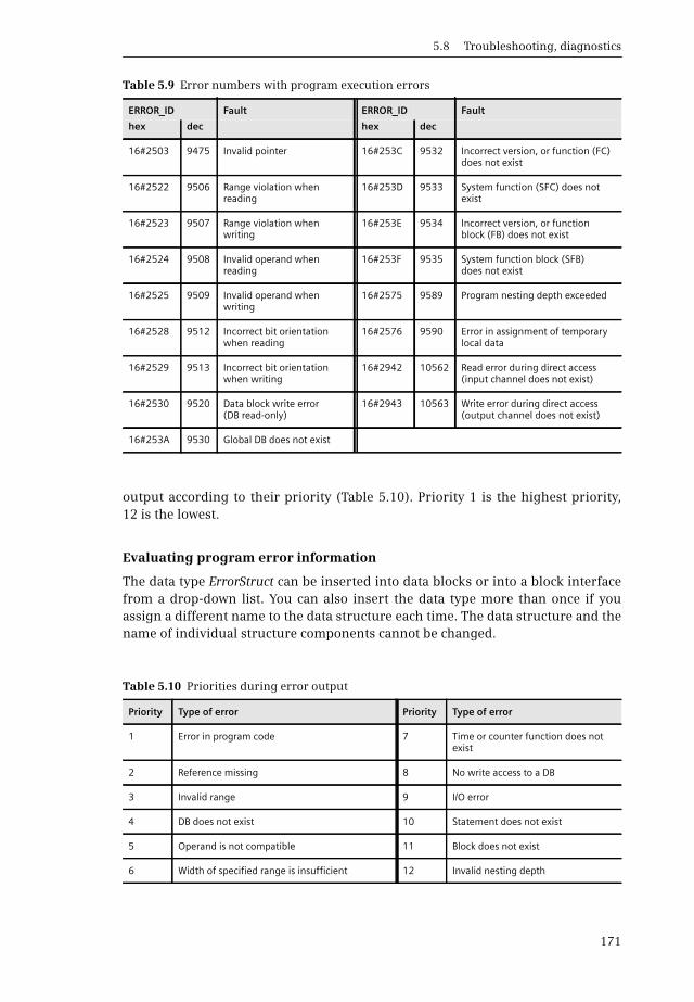
5.8 Troubleshooting, diagnostics
171
output according to their priority (Table 5.10). Priority 1 is the highest priority,12 is the lowest.
Evaluating program error information
The data type ErrorStruct can be inserted into data blocks or into a block interfacefrom a drop-down list. You can also insert the data type more than once if youassign a different name to the data structure each time. The data structure and thename of individual structure components cannot be changed.
Table 5.9 Error numbers with program execution errors
ERROR_ID Fault ERROR_ID Fault
hex dec hex dec
16#2503 9475 Invalid pointer 16#253C 9532 Incorrect version, or function (FC) does not exist
16#2522 9506 Range violation whenreading
16#253D 9533 System function (SFC) does not exist
16#2523 9507 Range violation when writing
16#253E 9534 Incorrect version, or function block (FB) does not exist
16#2524 9508 Invalid operand when reading
16#253F 9535 System function block (SFB) does not exist
16#2525 9509 Invalid operand when writing
16#2575 9589 Program nesting depth exceeded
16#2528 9512 Incorrect bit orientation when reading
16#2576 9590 Error in assignment of temporary local data
16#2529 9513 Incorrect bit orientation when writing
16#2942 10562 Read error during direct access (input channel does not exist)
16#2530 9520 Data block write error (DB read-only)
16#2943 10563 Write error during direct access (output channel does not exist)
16#253A 9530 Global DB does not exist
Table 5.10 Priorities during error output
Priority Type of error Priority Type of error
1 Error in program code 7 Time or counter function does not exist
2 Reference missing 8 No write access to a DB
3 Invalid range 9 I/O error
4 DB does not exist 10 Statement does not exist
5 Operand is not compatible 11 Block does not exist
6 Width of specified range is insufficient 12 Invalid nesting depth
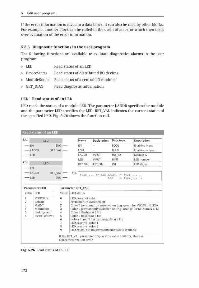
5 Edit user program
172
If the error information is saved in a data block, it can also be read by other blocks.For example, another block can be called in the event of an error which then takesover evaluation of the error information.
5.8.5 Diagnostic functions in the user program
The following functions are available to evaluate diagnostics alarms in the userprogram:
b LED Read status of an LED
b DeviceStates Read status of distributed I/O devices
b ModuleStates Read status of a central I/O modules
b GET_DIAG Read diagnostic information
LED Read status of an LED
LED reads the status of a module LED. The parameter LADDR specifies the moduleand the parameter LED specifies the LED. RET_VAL indicates the current status ofthe specified LED. Fig. 5.26 shows the function call.
Fig. 5.26 Read status of an LED
DeclarationName
EN
ENO
LADDR
LED
RET_VAL
–
–
INPUT
INPUT
RETURN
BOOL
BOOL
HW_IO
UINT
INT
Enabling input
Enabling output
Module ID
LED number
LED status
DescriptionData typeLED
Parameter LED Parameter RET_VAL
LED
EN
LADDR
LED
EN
LADDR
LED
ENO
RET_VAL
RET_VAL
ENO
LAD
FBD
Read status of an LED
SCL#var_... := LED(LADDR := #var_... ,
LED := #var_... );
Value LED
STOP/RUN2 ERROR1
3 MAINT4 redundant5 Link (green)6 Rx/Tx (yellow)
Value LED status
0 LED does not exist1 Permanently switched off
3Color 1 flashes at 2 Hz
56 Colors 1 and 2 flash alternately at 2 Hz7 LED is active, color 18 LED is active, color 29 LED exists, but no status information is available
If the RET_VAL parameter displays the value 16#80xx, there is a parameterization error.
Color 2 flashes at 2 Hz
Color 1 permanently switched on (e.g. green for STOP/RUN LED)
4
2Color 2 permanently switched on (e.g. orange for STOP/RUN LED)
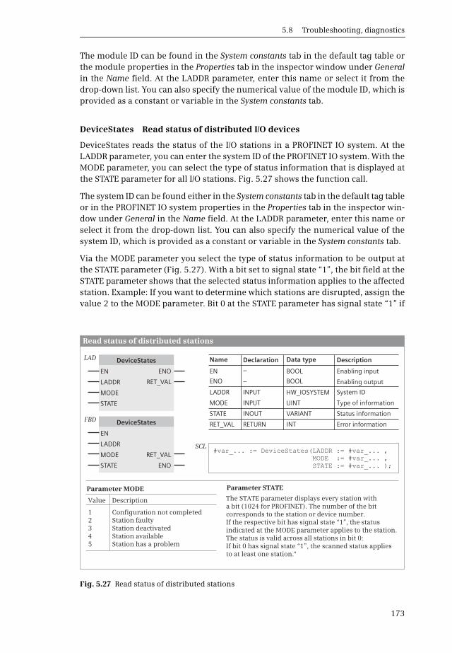
5.8 Troubleshooting, diagnostics
173
The module ID can be found in the System constants tab in the default tag table orthe module properties in the Properties tab in the inspector window under Generalin the Name field. At the LADDR parameter, enter this name or select it from thedrop-down list. You can also specify the numerical value of the module ID, which isprovided as a constant or variable in the System constants tab.
DeviceStates Read status of distributed I/O devices
DeviceStates reads the status of the I/O stations in a PROFINET IO system. At theLADDR parameter, you can enter the system ID of the PROFINET IO system. With theMODE parameter, you can select the type of status information that is displayed atthe STATE parameter for all I/O stations. Fig. 5.27 shows the function call.
The system ID can be found either in the System constants tab in the default tag tableor in the PROFINET IO system properties in the Properties tab in the inspector win-dow under General in the Name field. At the LADDR parameter, enter this name orselect it from the drop-down list. You can also specify the numerical value of thesystem ID, which is provided as a constant or variable in the System constants tab.
Via the MODE parameter you select the type of status information to be output atthe STATE parameter (Fig. 5.27). With a bit set to signal state “1”, the bit field at theSTATE parameter shows that the selected status information applies to the affectedstation. Example: If you want to determine which stations are disrupted, assign thevalue 2 to the MODE parameter. Bit 0 at the STATE parameter has signal state “1” if
Fig. 5.27 Read status of distributed stations
DeclarationName
EN
ENO
LADDR
MODE
STATE
RET_VAL
–
–
INPUT
INPUT
INOUT
RETURN
BOOL
BOOL
HW_IOSYSTEM
UINT
VARIANT
INT
Enabling input
Enabling output
System ID
Type of information
Status information
Error information
DescriptionData typeDeviceStates
DeviceStates
EN
LADDR
MODE
STATE
EN
LADDR
MODE
STATE
ENO
RET_VAL
RET_VAL
ENO
LAD
FBD
Read status of distributed stations
SCL#var_... := DeviceStates(LADDR := #var_... ,
MODE := #var_... ,STATE := #var_... );
Parameter MODE Parameter STATE
Value Description
1 Configuration not completed2 Station faulty3 Station deactivated4 Station available5 Station has a problem
The STATE parameter displays every station with a bit (1024 for PROFINET). The number of the bit corresponds to the station or device number. If the respective bit has signal state “1”, the status indicated at the MODE parameter applies to the station. The status is valid across all stations in bit 0: If bit 0 has signal state “1”, the scanned status applies to at least one station."
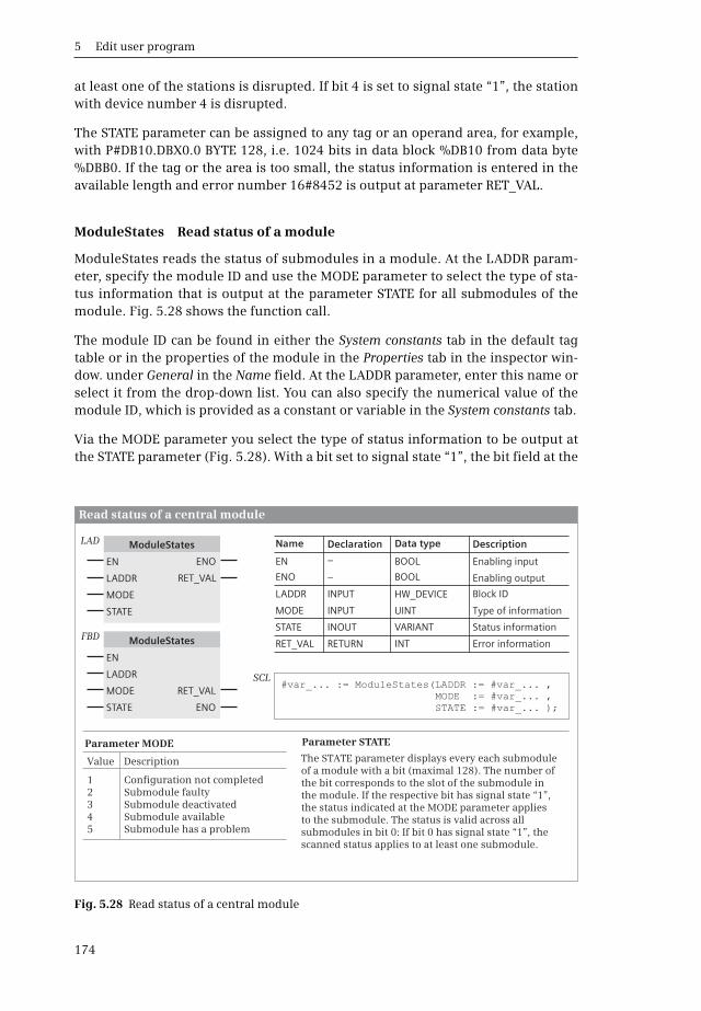
5 Edit user program
174
at least one of the stations is disrupted. If bit 4 is set to signal state “1”, the stationwith device number 4 is disrupted.
The STATE parameter can be assigned to any tag or an operand area, for example,with P#DB10.DBX0.0 BYTE 128, i.e. 1024 bits in data block %DB10 from data byte%DBB0. If the tag or the area is too small, the status information is entered in theavailable length and error number 16#8452 is output at parameter RET_VAL.
ModuleStates Read status of a module
ModuleStates reads the status of submodules in a module. At the LADDR param-eter, specify the module ID and use the MODE parameter to select the type of sta-tus information that is output at the parameter STATE for all submodules of themodule. Fig. 5.28 shows the function call.
The module ID can be found in either the System constants tab in the default tagtable or in the properties of the module in the Properties tab in the inspector win-dow. under General in the Name field. At the LADDR parameter, enter this name orselect it from the drop-down list. You can also specify the numerical value of themodule ID, which is provided as a constant or variable in the System constants tab.
Via the MODE parameter you select the type of status information to be output atthe STATE parameter (Fig. 5.28). With a bit set to signal state “1”, the bit field at the
Fig. 5.28 Read status of a central module
DeclarationName
EN
ENO
LADDR
MODE
STATE
RET_VAL
–
–
INPUT
INPUT
INOUT
RETURN
BOOL
BOOL
HW_DEVICE
UINT
VARIANT
INT
Enabling input
Enabling output
Block ID
Type of information
Status information
Error information
DescriptionData typeModuleStates
ModuleStates
EN
LADDR
MODE
STATE
EN
LADDR
MODE
STATE
ENO
RET_VAL
RET_VAL
ENO
LAD
FBD
SCL#var_... := ModuleStates(LADDR := #var_... ,
MODE := #var_... ,STATE := #var_... );
Parameter MODE Parameter STATE
Value Description
1 Configuration not completed2 Submodule faulty345
Submodule deactivatedSubmodule availableSubmodule has a problem
The STATE parameter displays every each submodule of a module with a bit (maximal 128). The number of the bit corresponds to the slot of the submodule in the module. If the respective bit has signal state “1”, the status indicated at the MODE parameter applies to the submodule. The status is valid across all submodules in bit 0: If bit 0 has signal state “1”, the scanned status applies to at least one submodule.
Read status of a central module
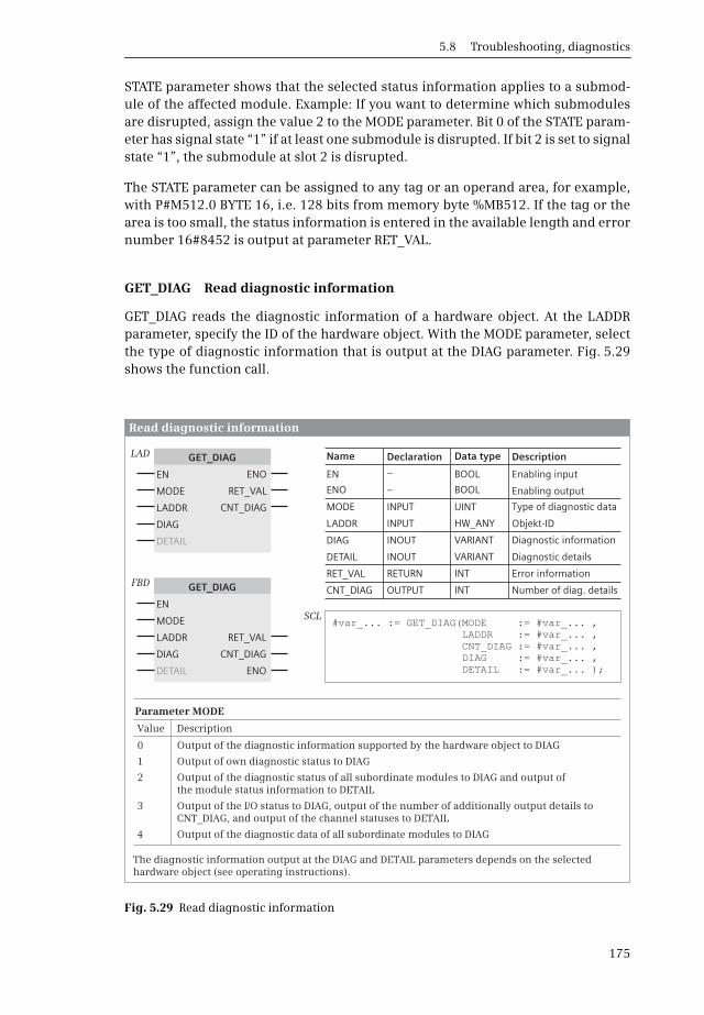
5.8 Troubleshooting, diagnostics
175
STATE parameter shows that the selected status information applies to a submod-ule of the affected module. Example: If you want to determine which submodulesare disrupted, assign the value 2 to the MODE parameter. Bit 0 of the STATE param-eter has signal state “1” if at least one submodule is disrupted. If bit 2 is set to signalstate “1”, the submodule at slot 2 is disrupted.
The STATE parameter can be assigned to any tag or an operand area, for example,with P#M512.0 BYTE 16, i.e. 128 bits from memory byte %MB512. If the tag or thearea is too small, the status information is entered in the available length and errornumber 16#8452 is output at parameter RET_VAL.
GET_DIAG Read diagnostic information
GET_DIAG reads the diagnostic information of a hardware object. At the LADDRparameter, specify the ID of the hardware object. With the MODE parameter, selectthe type of diagnostic information that is output at the DIAG parameter. Fig. 5.29shows the function call.
Fig. 5.29 Read diagnostic information
Read diagnostic information
DeclarationName
EN
ENO
MODE
LADDR
DIAG
DETAIL
RET_VAL
CNT_DIAG
–
–
INPUT
INPUT
INOUT
INOUT
RETURN
OUTPUT
BOOL
BOOL
UINT
HW_ANY
VARIANT
VARIANT
INT
INT
Enabling input
Enabling output
Type of diagnostic data
Objekt-ID
Diagnostic information
Diagnostic details
Error information
Number of diag. details
DescriptionData typeGET_DIAG
GET_DIAG
EN
MODE
DIAG
LADDR
DETAIL
EN
MODE
DIAG
LADDR
DETAIL
ENO
RET_VAL
CNT_DIAG
CNT_DIAG
RET_VAL
ENO
LAD
FBD
SCL#var_... := GET_DIAG(MODE := #var_... ,
LADDR := #var_... ,CNT_DIAG := #var_... ,DIAG := #var_... ,DETAIL := #var_... );
Parameter MODE
Value Description
0 Output of the diagnostic information supported by the hardware object to DIAG
1 Output of own diagnostic status to DIAG
2 Output of the diagnostic status of all subordinate modules to DIAG and output of the module status information to DETAIL
3
4
Output of the I/O status to DIAG, output of the number of additionally output details to CNT_DIAG, and output of the channel statuses to DETAIL
Output of the diagnostic data of all subordinate modules to DIAG
The diagnostic information output at the DIAG and DETAIL parameters depends on the selected hardware object (see operating instructions).
5 Edit user program
176
The object ID can be found either in the System constants tab in the default tag tableor in the properties of the hardware object in the Properties tab in the inspector win-dow under General in the Name field. At the LADDR parameter, enter this name orselect it from the drop-down list. You can also specify the numerical value of theobject ID, which is provided as a constant or variable in the System constants tab.
Via the MODE parameter you select the type of information to be output at theDIAG parameter (Fig. 5.29). The value 0 is used to query what diagnostic informa-tion the hardware object supports. Each bit set to signal state “1” at the DIAGparameter corresponds to an assignment of the MODE parameter: If the bit 1 is set,MODE = 1 is supported. If the bit 2 is set, MODE = 2 is supported, etc. CNT_DIAG isset to value 0; DETAIL is not changed.
If MODE = 1, the diagnostic information of the selected hardware object is output atparameter DIAG. CNT_DIAG is set to value 0, DETAIL is not changed.
If MODE = 2, the diagnostic status of all the modules in the hardware object is out-put at parameter DIAG. CNT_DIAG is set to value 1, DETAIL contains module stateinformation.
If MODE = 3, the state of the inputs and outputs of the selected hardware object isoutput at parameter DIAG. CNT_DIAG is set to the number of module channelswhose status data is output at the parameter DETAIL.
If MODE = 4, the state of the inputs and outputs of all modules in the hardwareobject is output at parameter DIAG. CNT_DIAG is set to value 0, DETAIL is notchanged.
5.8.6 Diagnostics interrupt OB 82
Appropriately designed modules can detect diagnostics events, for example“No load voltage present” (I/O modules), overshoot and undershoot, wire breakand short-circuit (analog input modules). If the detection of a diagnostics event isactivated in the device configuration editor, the organization block OB 82 Diag-nostics interrupt is called when the event occurs.
The diagnostics interrupt organization block is assigned to event class Diagnosticerror interrupt. It is of hardware data type OB_DIAG. The System constants tab of thedefault tag table lists the name and value of the constant. The name of the constantcan be changed in the block properties.
You can only use one diagnostics interrupt OB in your program.
The OB 82 is processed if no other interrupt organization block is active, otherwisethe diagnostics event is entered into the queue.
When a diagnostics event occurs, it is written into the diagnostics buffer. If an OB 82is not present when a diagnostics event occurs, the CPU ignores the event.
Calling of the diagnostics interrupt OB can be delayed or enabled using theDIS_AIRT and EN_AIRT functions.
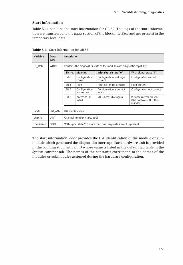
5.8 Troubleshooting, diagnostics
177
Start information
Table 5.11 contains the start information for OB 82. The tags of the start informa-tion are transferred to the Input section of the block interface and are present in thetemporary local data.
The start information laddr provides the HW identification of the module or sub-module which generated the diagnostics interrupt. Each hardware unit is providedin the configuration with an ID whose value is listed in the default tag table in theSystem constant tab. The names of the constants correspond to the names of themodules or submodules assigned during the hardware configuration.
Table 5.11 Start information for OB 82
Variable Data type
Description
IO_state WORD Contains the diagnostics state of the module with diagnostic capability
laddr HW_ANY HW identification
channel UINT Channel number (starts at 0)
multi-error BOOL With signal state “1”, more than one diagnostics event is present
Bit no. Meaning With signal state “0” With signal state “1”
Bit 0 Configuration correct
Configuration no longer correct
Configuration correct
Bit 4 Fault Fault no longer present Fault present
Bit 5 Configuration not correct
Configuration is correct again
Configuration not correct
Bit 6 Access to I/O failed
I/O is accessible again I/O access error present (the hardware ID is then in laddr)
6 Program editor
178
6 Program editor
6.1 Introduction
This chapter describes how to work with the program editor, with which the userprogram is written in the programming languages LAD, FBD, and SCL. The specialfeatures of programming in the respective programming language are described inthe Chapters 7 “Ladder logic LAD” on page 209, 8 “Function block diagram FBD” onpage 246, and 9 “Structured Control Language SCL” on page 284.
The user program consists of blocks which are saved in the project tree under a PLCstation in the Program blocks folder. Logic blocks contain the program code, anddata blocks contain the control data. When programming, a block is initially cre-ated and subsequently filled with data or a program. The programming languagesladder logic (LAD), function block diagram (FBD), and structured control language(SCL) are available for programming the control function. You can define the pro-gramming language individually for each block.
The user program works with operands and tags. Block-local tags are declaredduring programming of the blocks, global operands and tags are present in the PLCtags folder. The PLC data types folder contains user-defined data structures for tagsand data blocks.
Programming is appropriately commenced by definition of PLC tags and PLC datatypes. This is followed by the global data blocks with the already known data. Forthe logic blocks, one starts with those which are at the lowest position in the callhierarchy. The blocks in the next higher level in the hierarchy then call the blockspositioned below them. The organization blocks in the highest hierarchy level arecreated last.
The program editor makes various tools available to support you in program cre-ation and testing. The cross-reference list contains the already programmed tagsand blocks and the point in the program where they are used. The assignment listshows the current use of the inputs, outputs, and bit memories. The call and depen-dency structure shows the sequence the blocks are called.
Following completion, the user program is compiled, i.e. the program editor con-verts the data entered into a program which can be executed on the CPU.
6.2 PLC tag table
You work in the user program with operands which are e.g. inputs or outputs. Theseoperands can be addressed in absolute mode (e.g. %I1.0) or symbolic mode(e.g. “Start signal”). Symbolic addressing uses names (identifiers) instead of the ab-

6.2 PLC tag table
179
solute address. As well as the name, you define the data type of the operand. Thecombination of operand (absolute address, memory location), name, and data typeis referred to as a “tag”.
When writing the user program, a distinction is made between local and global tags.A local tag is only known in the block in which it has been defined. You can use localtags with the same name in different blocks for different purposes. A global tag isknown throughout the entire user program, and has the same meaning in allblocks. You define global tags in the PLC tag table.
Refer to Chapter 6.6.1 “Cross-reference list” on page 201 for how to create a cross-reference list of the PLC tags. Monitoring of tags using the PLC tag table is describedin Chapter 13.4.4 “Monitoring with the PLC tag table” on page 445.
6.2.1 Creating and editing the PLC tag table
When creating a PLC station, a PLC tags folder with the PLC tag table is also created.You can open the PLC tag table by double-clicking on Default tag table in the PLCtags folder. The default tag table consists of the Tags, User constants, and Systemconstants tabs.
You can create additional tag tables containing PLC tags and user constants with theAdd new tag table function. These self-created tables can be renamed and organizedin groups. A tag or a constant can only be defined in one of the tables. To obtain anoverview of all tags and constants, double-click on Show all tags in the PLC tagsfolder.
You can save an incomplete or faulty PLC tag table at any time and process it againlater. However, the tag table must be error-free to enable compilation of the userprogram.
6.2.2 Defining PLC tags
In the Tags tab, enter the name, data type, and address (operand, memory location)of the tags used. The name can contain letters, digits, and special characters (noquotation marks). It must not already have been assigned for a different PLC tag, asymbolically addressed constant, a PLC data type, or a block. No distinction is madebetween upper and lower case when checking the name.
You can add an explanatory comment to each defined tag. Table 6.1 contains theoperands and data types permissible as PLC tags. The data type defines certainproperties of the data associated with the name, basically the representation of thedata content. An overview of the data types used with a CPU 1200 and the detaileddescription can be found in Chapter 4 “Variables and data types” on page 79.
Part of the operand area Bit memory can be set to retentive, i.e. this part retains thesignal statuses and values following a power off and subsequent power on. To setthe retain area, click in the toolbar of the PLC tags table on the Retain symbol andenter the number of retentive memory bytes in the dialog which is then displayed.

6 Program editor
180
A tick in the Retain column then identifies which bit memory operands are reten-tive.
The properties of a PLC tag include the attributes
b Accessible from HMIWhen activated, an HMI station can access this tag during runtime.
b Visible in HMIWhen activated, this tag is visible by default in the selection list of an HMI station.
Fig. 6.1 shows an example of a PLC tag table.
Table 6.1 Approved operands and data types for PLC tags
Input operand
Output operand
Bit memory operand
Approved data types
Address range
Input bit I Output bit Q Memory bit M BOOL I, Q: 0.01023.7M: 0.04095.7 1)M: 0.08191.7 2)
Input byte IB Output byte QB Memory byte MB BYTE, CHAR, SINT, USINT
IB, QB: 01023MB: 04095 1)MB: 08191 2)
Input word IW Output word QW Memory word FW WORD, INT, UINT IW, QW: 01022MW: 04094 1)MW: 08190 2)
Input double word ID
Output double word QD
Memory double word MD
DWORD, DINT, UDINT, REAL, TIME
ID, QD: 01020MD: 04092 1)MD: 08188 2)
1) For CPU 1211 and CPU 1212 2) For CPU 1214 and CPU 1215
Fig. 6.1 Example of a PLC tag table

6.2 PLC tag table
181
6.2.3 Editing a PLC tag table
You can use Insert row from the shortcut menu to insert an empty line above theselected line. Add row inserts a line after the selected line. The Delete commanddeletes the selected line. You can copy selected lines and add them to the end of thelist. You can sort the lines according to the column contents by clicking the headerof the appropriate column. Sorting is in ascending order with the first click, indescending order with the second click, and the original state is reestablished fol-lowing the third click.
To fill out the table automatically, select the name of the tag to be transferred, posi-tion the cursor at the bottom right corner of the cell, and drag downward over thelines with the mouse button pressed.
If you enter the same name a second time, for example when copying lines, a con-secutive number in parentheses is appended to the name. When filling out auto-matically, this is an underscore character with a consecutive number. Doubleassignment of an address is indicated by a colored background.
You can also supplement, change or delete the PLC tags when entering the user pro-gram (described in Chapter 6.3.6 “Editing tags” on page 192).
In addition to the default tag table, which is always available, you can create furtherPLC tag tables. In doing so, you may not give a tag multiple definitions. If you dou-ble-click on Show all tags, the program editor creates an overview of the tags of allof the tag tables.
You can compare a PLC tag table with one from another project if you mark the tagtable and select the command Tools > Compare > Offline/offline.
6.2.4 Exporting and importing a PLC tag table
A PLC tag table can also be created or edited using an external editor. The externalfile is present in .xlsx format.
To export, open the PLC tag table and select the Export icon in the toolbar. Set thefile name and path in the dialog, and select the data to be exported (tags or con-stants). The contents of the opened PLC tag table are exported. To export all PLCtags, open the complete table by double-clicking on Show all tags and then selectthe Export icon.
The external file contains the PLC tags worksheet for the PLC tags and the Constantsworksheet for the symbolically addressed user constants (Table 6.2).
To import, double-click on Show all tags under the PLC station in the PLC tags folderin the project tree. Select the Import icon in the toolbar. Set the file name and pathin the dialog, and select the data to be imported (tags or constants). The contents ofthe external file are imported into the tag table, which is specified in the Path col-umn. Existing entries are identified by a consecutive number in parenthesesappended to the name and/or by an address highlighted in color.
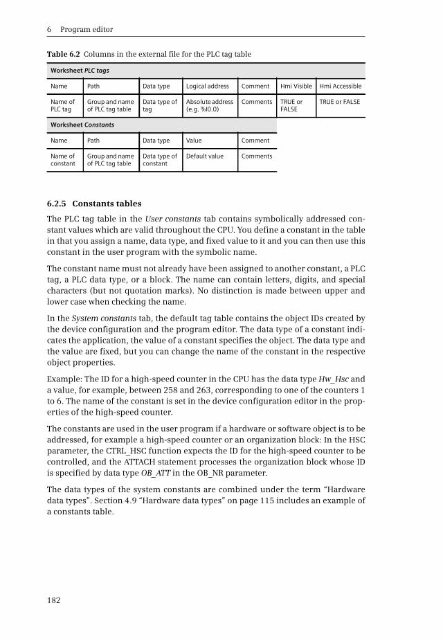
6 Program editor
182
6.2.5 Constants tables
The PLC tag table in the User constants tab contains symbolically addressed con-stant values which are valid throughout the CPU. You define a constant in the tablein that you assign a name, data type, and fixed value to it and you can then use thisconstant in the user program with the symbolic name.
The constant name must not already have been assigned to another constant, a PLCtag, a PLC data type, or a block. The name can contain letters, digits, and specialcharacters (but not quotation marks). No distinction is made between upper andlower case when checking the name.
In the System constants tab, the default tag table contains the object IDs created bythe device configuration and the program editor. The data type of a constant indi-cates the application, the value of a constant specifies the object. The data type andthe value are fixed, but you can change the name of the constant in the respectiveobject properties.
Example: The ID for a high-speed counter in the CPU has the data type Hw_Hsc anda value, for example, between 258 and 263, corresponding to one of the counters 1to 6. The name of the constant is set in the device configuration editor in the prop-erties of the high-speed counter.
The constants are used in the user program if a hardware or software object is to beaddressed, for example a high-speed counter or an organization block: In the HSCparameter, the CTRL_HSC function expects the ID for the high-speed counter to becontrolled, and the ATTACH statement processes the organization block whose IDis specified by data type OB_ATT in the OB_NR parameter.
The data types of the system constants are combined under the term “Hardwaredata types”. Section 4.9 “Hardware data types” on page 115 includes an example ofa constants table.
Table 6.2 Columns in the external file for the PLC tag table
Worksheet PLC tags
Name Path Data type Logical address Comment Hmi Visible Hmi Accessible
Name of PLC tag
Group and name of PLC tag table
Data type of tag
Absolute address (e.g. %I0.0)
Comments TRUE or FALSE
TRUE or FALSE
Worksheet Constants
Name Path Data type Value Comment
Name of constant
Group and name of PLC tag table
Data type of constant
Default value Comments
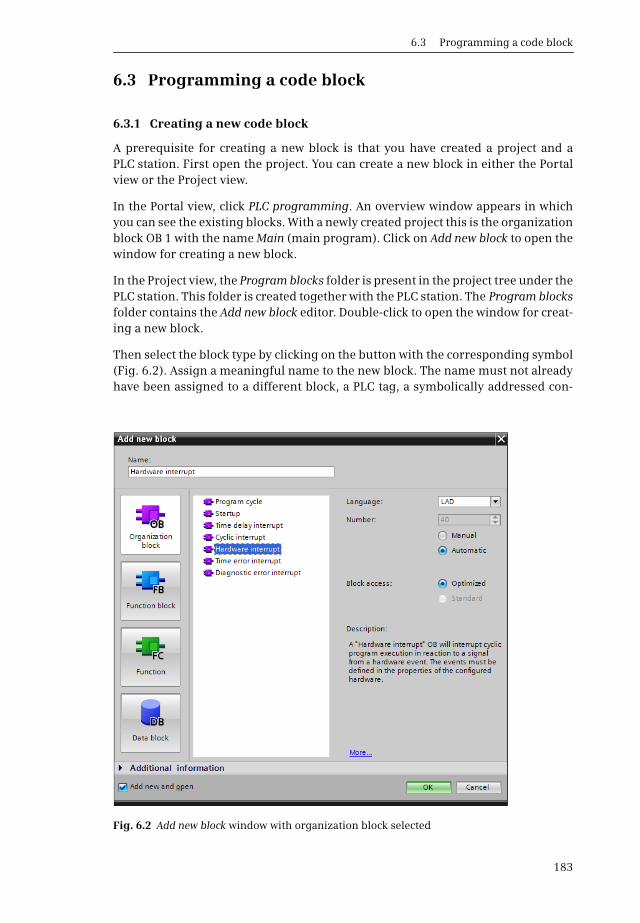
6.3 Programming a code block
183
6.3 Programming a code block
6.3.1 Creating a new code block
A prerequisite for creating a new block is that you have created a project and aPLC station. First open the project. You can create a new block in either the Portalview or the Project view.
In the Portal view, click PLC programming. An overview window appears in whichyou can see the existing blocks. With a newly created project this is the organizationblock OB 1 with the name Main (main program). Click on Add new block to open thewindow for creating a new block.
In the Project view, the Program blocks folder is present in the project tree under thePLC station. This folder is created together with the PLC station. The Program blocksfolder contains the Add new block editor. Double-click to open the window for creat-ing a new block.
Then select the block type by clicking on the button with the corresponding symbol(Fig. 6.2). Assign a meaningful name to the new block. The name must not alreadyhave been assigned to a different block, a PLC tag, a symbolically addressed con-
Fig. 6.2 Add new block window with organization block selected

6 Program editor
184
stant, and a PLC data type. The name can contain letters, digits, and special charac-ters (but not quotation marks). No distinction is made between upper and lower casewhen checking the name.
Then select the programming language for the block. With automatic assignmentof the block numbers, the lowest free number for the type of block is displayed ineach case. If you select the Manual option, you can enter a different number. TheOptimized option activates the Optimized block access attribute and has effects onaddressing, the retentivity, and the data types of the tags used in the block. Activa-tion of the check box is recommended.
You must assign an event class to an organization block, i.e. you specify the type oforganization block. Select the event class from the displayed list. Depending on theevent class, the block number is either fixed or freely-selectable. You can createmultiple organization blocks with different numbers for some event classes (seeChapter 5.7.1 “Introduction to interrupt processing” on page 153).
You set the default setting when creating a new block in the main menu in the Proj-ect view using the Options > Settings command in the PLC programming section.Under General and Default setting for new blocks, you can set the preselection for IECcheck and Optimized block access.
If the Add new and open checkbox is activated in the Add new block window, the pro-gram editor is started and programming of the newly created block can begin.
6.3.2 Working area of program editor for code blocks
The program editor is automatically started when a block is opened. Open a blockby double-clicking on its symbol: this can be found in the Portal view in the over-view window of the PLC programming, and in the Project view in the Programblocks folder under the PLC station in the project tree.
You can adapt the properties of the program editor according to your requirementsusing the Options > Settings command in the main menu. Select the PLC program-ming section, and set the font size, layout and width of the operand field underLAD/FBD.
The program editor displays the opened block with interface and program in theworking window (Fig. 6.3). Prior to programming, the block properties are presentin the inspector window; during programming, the properties of the selected oredited object are present here. The task window contains the program elements cat-alog in the Statements task card.
The working window of the program editor shows the following details:
b The toolbarcontains the symbols for the programming menu commands (e.g. Insert net-work, Delete network, Go to next error, etc.). The meaning of the symbols is dis-played if you hold the mouse pointer over the symbol. Currently non-selectableicons are grayed out.

6.3 Programming a code block
185
b The interfaceshows the block interface with the block parameters and the block-local tags.
b The favorites barprovides the favorite program elements (instructions), which can also be foundin the Favorites section of the program elements catalog. You can activate anddeactivate the display in the editor: Click with the right mouse button in thefavorites catalog or favorites bar and activate or deactivate Display favorites ineditor. To add a instruction to the favorites, select the instruction in the programelements catalog and drag and drop it with the mouse into the favorites catalogor favorites bar. To remove a instruction from the favorites, click with the rightmouse button and then select Remove instruction.
b The block windowcontains the block program. Enter the control function of the block here.
Fig. 6.3 Example of the program editor's working window in ladder logic
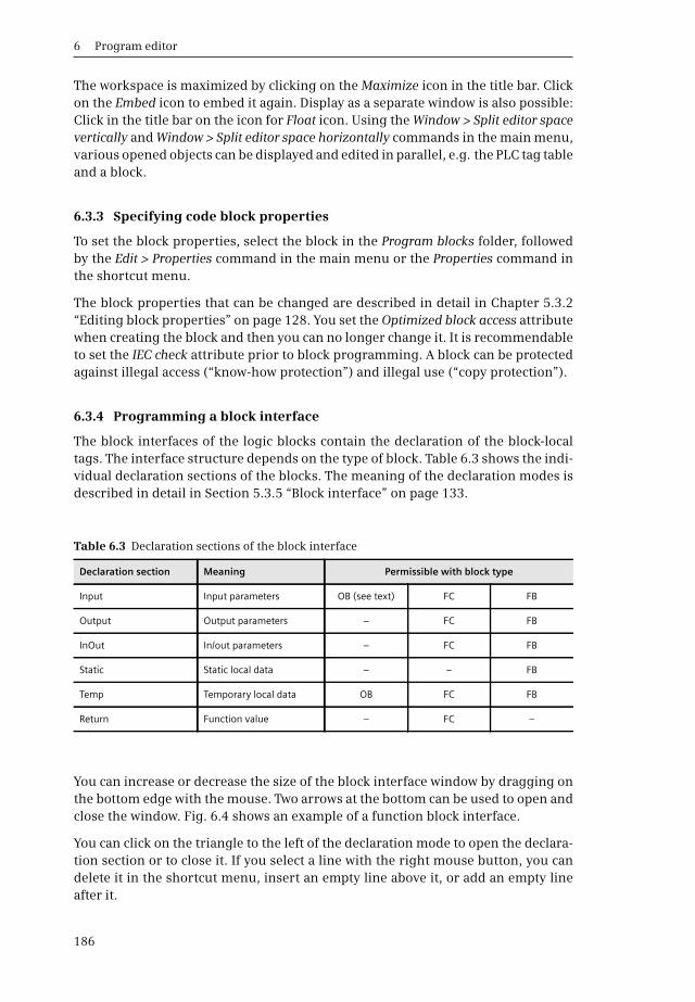
6 Program editor
186
The workspace is maximized by clicking on the Maximize icon in the title bar. Clickon the Embed icon to embed it again. Display as a separate window is also possible:Click in the title bar on the icon for Float icon. Using the Window > Split editor spacevertically and Window > Split editor space horizontally commands in the main menu,various opened objects can be displayed and edited in parallel, e.g. the PLC tag tableand a block.
6.3.3 Specifying code block properties
To set the block properties, select the block in the Program blocks folder, followedby the Edit > Properties command in the main menu or the Properties command inthe shortcut menu.
The block properties that can be changed are described in detail in Chapter 5.3.2“Editing block properties” on page 128. You set the Optimized block access attributewhen creating the block and then you can no longer change it. It is recommendableto set the IEC check attribute prior to block programming. A block can be protectedagainst illegal access (“know-how protection”) and illegal use (“copy protection”).
6.3.4 Programming a block interface
The block interfaces of the logic blocks contain the declaration of the block-localtags. The interface structure depends on the type of block. Table 6.3 shows the indi-vidual declaration sections of the blocks. The meaning of the declaration modes isdescribed in detail in Section 5.3.5 “Block interface” on page 133.
You can increase or decrease the size of the block interface window by dragging onthe bottom edge with the mouse. Two arrows at the bottom can be used to open andclose the window. Fig. 6.4 shows an example of a function block interface.
You can click on the triangle to the left of the declaration mode to open the declara-tion section or to close it. If you select a line with the right mouse button, you candelete it in the shortcut menu, insert an empty line above it, or add an empty lineafter it.
Table 6.3 Declaration sections of the block interface
Declaration section Meaning Permissible with block type
Input Input parameters OB (see text) FC FB
Output Output parameters – FC FB
InOut In/out parameters – FC FB
Static Static local data – – FB
Temp Temporary local data OB FC FB
Return Function value – FC –

6.3 Programming a code block
187
The name can contain letters, digits, and special characters (but not quotationmarks). No distinction is made between upper and lower case when checking thename. A drop-down list shows the currently permissible data types. You can use thecomment to describe the purpose of the respective tag.
The Default value column is displayed for a function block (FB). You can enter adefault value here which is saved in the instance data block. The Retain column isdisplayed in the interface of function blocks if the Optimized block access attributeis activated in the block. Here you can set the retentivity for individual tag values(Non-retentive, Retentive, Set in IDB). If Optimized block access is not activated, theretentivity can only be set in the instance data block, and only for the completeinterface.
Neither a default value nor the retentivity can be set for the temporary local data.
The organization blocks OB 80 Time error, OB 82 Diagnostics interrupt, and OB 100Startup program as well as all other organization blocks of event class Startup pro-vide start information for the user program. Although this start information islocated in the CPU's system memory like the temporary local data, it is shown in thedeclaration section Input.
In the case of a function (FC), the function value with the name Ret_Val and datatype VOID is displayed in the interface in the Return section. The function value hasno significance when programming with ladder logic and function block diagram.
Fig. 6.4 Example of function block interface

6 Program editor
188
The data type VOID prevents the display in the call box. If you specify a differentdata type here, the function value is treated like the first output parameter. Usingthe SCL programming language, you can integrate a function in an expressioninstead of a tag with the data type of the function value (see Section “Using a func-tion value of a function (FC)” on page 139).
For logic blocks with deactivated Optimized block access attribute, tags in the blockinterface can be overlaid with other data types (see Chapter 4.3.3 “Overlaying tags(data type views)” on page 93).
6.3.5 Programming control functions
Working with networks
A network is part of a logic block which, in the case of the LAD and FBD program-ming languages, contains a complete current path or a complete logic operation.No networks are possible with SCL.
The program editor automatically numbers the networks starting from 1. You canassign a title and a comment to each network. When editing, you can directly selectany network from the main menu using the Edit > Go to > Network / line command.
The networks can be opened or closed. To do this, select Network with the rightmouse button and then select the Collapse or Expand command from the shortcutmenu, or click in the toolbar of the working window on the Close all networks orOpen all networks icon.
When programming the last network in each case, an empty network is automati-cally appended. To program a new network, select the Insert > Network commandfrom the shortcut menu. The editor then adds an empty network after the currentlyselected network.
You can show or hide the network comments using the Network comments on/officon in the toolbar or the View > Display with > Network comments command in themain menu.
Following each network, the tags used in the network can be shown with name,address, and comment. You can show or hide the tag information using the Taginformation on/off icon in the toolbar or the View > Display with > Tag informationcommand in the main menu.
The network comments and tag information view can be set for all blocks withthe command Options > Settings in the main menu under the group PLC Program-ming > View by activating the relevant option With comments and/or With tag in-formation.

6.3 Programming a code block
189
Program elements catalog
All program elements permissible for the respective programming language (con-tacts, coils, boxes, statements, etc.) can be found in the program elements catalogin the task window. The program elements catalog is divided into the followinggroups
b Favorites (frequently required program elements)
b Basic instructions (basic functions)
b Extended instructions (functions implemented by system blocks)
b Technology (technological functions, e.g. for PID controllers or high-speed counters)
b Communication (communication functions for data transmission and for communication modules).
You can combine a selection of frequently used program elements in the Favoritescatalog and display them in the favorites bar of the program editor to allow rapidselection.
General procedure when programming
To enter the program code, position the program elements in the desired arrange-ment and subsequently supply them with tags or enter the statement lines. Theprogram editor immediately checks your inputs and indicates faulty entries.
You can interrupt block programming at any time – even if the program is stillincomplete or faulty – and continue later. You can store a block by saving the com-plete project using the Project > Save command from the main menu.
You can save the structure of the windows and tables using the Save window settingsicon in the top right corner of the working window. This structure is reestablishedthe next time the working window is opened.
Programming a control function with ladder diagram (LAD)
To program the control function in LAD, select a program element in the catalogand drag it with the mouse into the open network under the network comment. Thefirst program element is positioned automatically. With the next program element,small boxes indicate where the new program element may be positioned and – ingreen – where it is positioned when you “drop” it.
In the ladder logic, the binary logic operations are implemented by series and par-allel connections (Fig. 6.5). With the ladder logic, the Q or ENO output is positionedin the display at the top edge of the box in order to be able to “hang” the box intothe current path. The structure of an LAD current path is described in Chapter 7“Ladder logic LAD” on page 209.
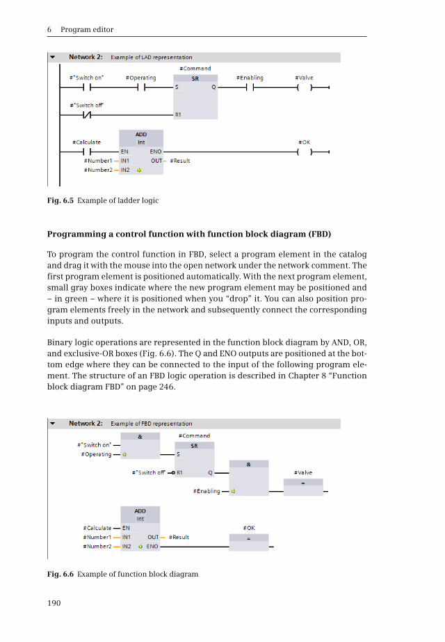
6 Program editor
190
Programming a control function with function block diagram (FBD)
To program the control function in FBD, select a program element in the catalogand drag it with the mouse into the open network under the network comment. Thefirst program element is positioned automatically. With the next program element,small gray boxes indicate where the new program element may be positioned and– in green – where it is positioned when you “drop” it. You can also position pro-gram elements freely in the network and subsequently connect the correspondinginputs and outputs.
Binary logic operations are represented in the function block diagram by AND, OR,and exclusive-OR boxes (Fig. 6.6). The Q and ENO outputs are positioned at the bot-tom edge where they can be connected to the input of the following program ele-ment. The structure of an FBD logic operation is described in Chapter 8 “Functionblock diagram FBD” on page 246.
Fig. 6.5 Example of ladder logic
Fig. 6.6 Example of function block diagram
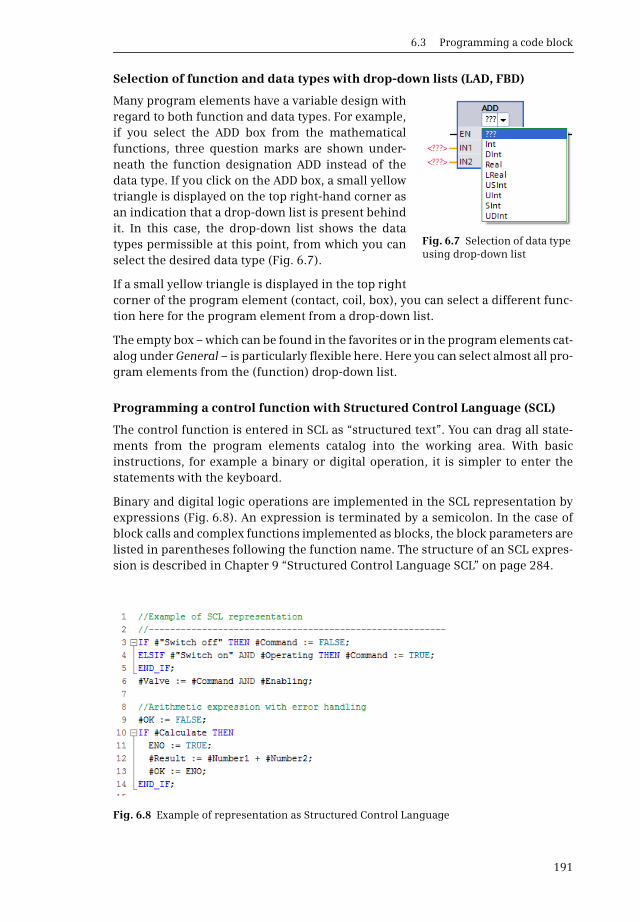
6.3 Programming a code block
191
Selection of function and data types with drop-down lists (LAD, FBD)
Many program elements have a variable design withregard to both function and data types. For example,if you select the ADD box from the mathematicalfunctions, three question marks are shown under-neath the function designation ADD instead of thedata type. If you click on the ADD box, a small yellowtriangle is displayed on the top right-hand corner asan indication that a drop-down list is present behindit. In this case, the drop-down list shows the datatypes permissible at this point, from which you canselect the desired data type (Fig. 6.7).
If a small yellow triangle is displayed in the top rightcorner of the program element (contact, coil, box), you can select a different func-tion here for the program element from a drop-down list.
The empty box – which can be found in the favorites or in the program elements cat-alog under General – is particularly flexible here. Here you can select almost all pro-gram elements from the (function) drop-down list.
Programming a control function with Structured Control Language (SCL)
The control function is entered in SCL as “structured text”. You can drag all state-ments from the program elements catalog into the working area. With basicinstructions, for example a binary or digital operation, it is simpler to enter thestatements with the keyboard.
Binary and digital logic operations are implemented in the SCL representation byexpressions (Fig. 6.8). An expression is terminated by a semicolon. In the case ofblock calls and complex functions implemented as blocks, the block parameters arelisted in parentheses following the function name. The structure of an SCL expres-sion is described in Chapter 9 “Structured Control Language SCL” on page 284.
Fig. 6.8 Example of representation as Structured Control Language
Fig. 6.7 Selection of data type using drop-down list
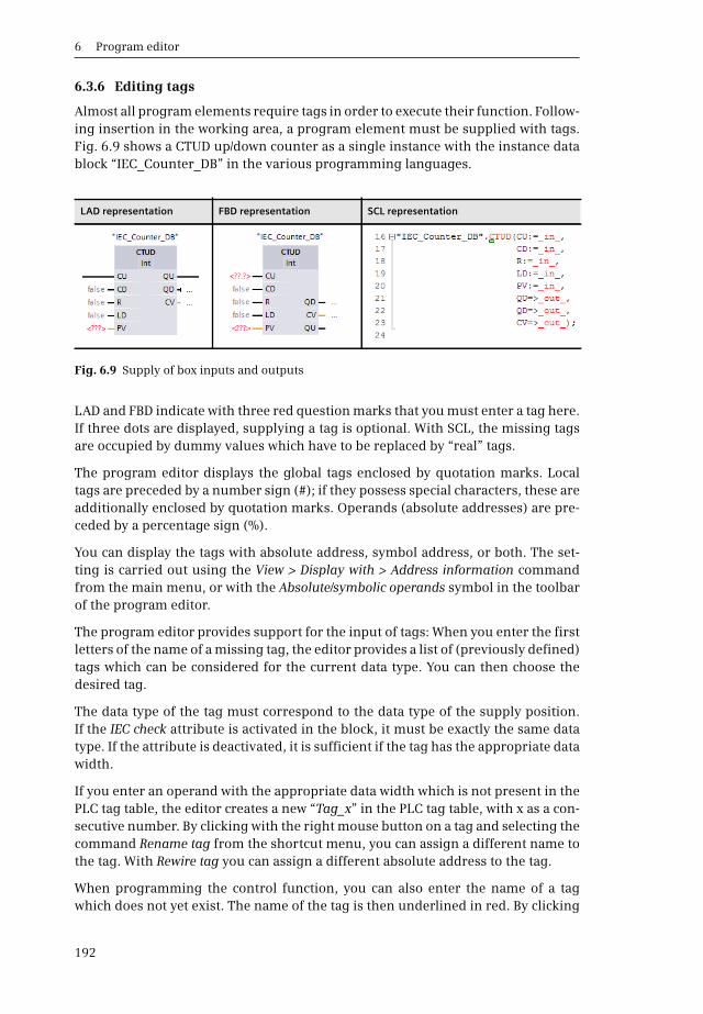
6 Program editor
192
6.3.6 Editing tags
Almost all program elements require tags in order to execute their function. Follow-ing insertion in the working area, a program element must be supplied with tags.Fig. 6.9 shows a CTUD up/down counter as a single instance with the instance datablock “IEC_Counter_DB” in the various programming languages.
LAD and FBD indicate with three red question marks that you must enter a tag here.If three dots are displayed, supplying a tag is optional. With SCL, the missing tagsare occupied by dummy values which have to be replaced by “real” tags.
The program editor displays the global tags enclosed by quotation marks. Localtags are preceded by a number sign (#); if they possess special characters, these areadditionally enclosed by quotation marks. Operands (absolute addresses) are pre-ceded by a percentage sign (%).
You can display the tags with absolute address, symbol address, or both. The set-ting is carried out using the View > Display with > Address information commandfrom the main menu, or with the Absolute/symbolic operands symbol in the toolbarof the program editor.
The program editor provides support for the input of tags: When you enter the firstletters of the name of a missing tag, the editor provides a list of (previously defined)tags which can be considered for the current data type. You can then choose thedesired tag.
The data type of the tag must correspond to the data type of the supply position.If the IEC check attribute is activated in the block, it must be exactly the same datatype. If the attribute is deactivated, it is sufficient if the tag has the appropriate datawidth.
If you enter an operand with the appropriate data width which is not present in thePLC tag table, the editor creates a new “Tag_x” in the PLC tag table, with x as a con-secutive number. By clicking with the right mouse button on a tag and selecting thecommand Rename tag from the shortcut menu, you can assign a different name tothe tag. With Rewire tag you can assign a different absolute address to the tag.
When programming the control function, you can also enter the name of a tagwhich does not yet exist. The name of the tag is then underlined in red. By clicking
LAD representation FBD representation SCL representation
Fig. 6.9 Supply of box inputs and outputs
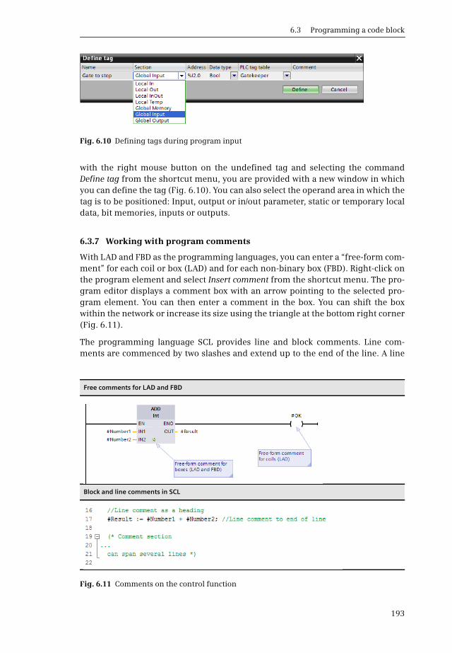
6.3 Programming a code block
193
with the right mouse button on the undefined tag and selecting the commandDefine tag from the shortcut menu, you are provided with a new window in whichyou can define the tag (Fig. 6.10). You can also select the operand area in which thetag is to be positioned: Input, output or in/out parameter, static or temporary localdata, bit memories, inputs or outputs.
6.3.7 Working with program comments
With LAD and FBD as the programming languages, you can enter a “free-form com-ment” for each coil or box (LAD) and for each non-binary box (FBD). Right-click onthe program element and select Insert comment from the shortcut menu. The pro-gram editor displays a comment box with an arrow pointing to the selected pro-gram element. You can then enter a comment in the box. You can shift the boxwithin the network or increase its size using the triangle at the bottom right corner(Fig. 6.11).
The programming language SCL provides line and block comments. Line com-ments are commenced by two slashes and extend up to the end of the line. A line
Fig. 6.10 Defining tags during program input
Free comments for LAD and FBD
Block and line comments in SCL
Fig. 6.11 Comments on the control function

6 Program editor
194
comment can also stand alone in a line, for example as a heading. A block commentis starts with left parenthesis and asterisk and ends with a asterisk and right paren-thesis. Example: (* This is a block comment *). It can extend over several lines.
In SCL, you can eliminate the comment in a code line by positioning the cursor inthe code line and clicking the Disable code icon in the toolbar of the working win-dow. Two slashes are then placed at the beginning of the code line. You can reversethe procedure using the Enable code icon.
6.4 Programming a data block
6.4.1 Creating a new data block
It is only possible to create a new data block if a project and a PLC station have firstbeen created. First open the project. You can create a new data block in either thePortal view or the Project view.
In the Portal view, click PLC programming and subsequently Add new block. In theProject view, double-click on Add new block in the Program blocks folder. In the win-dow for creating a new block, select the symbol for Data block.
Data blocks must be assigned a type:
b A global data block contains the tags which you specify when programming thedata block. You can design the contents and structure of the data block asdesired.
b An instance data block contains the block parameters and static local data of afunction block (FB). The data structure is specified when programming the blockinterface. For instance data blocks for system functions, the structure is alreadyspecified and cannot be changed.
b A data block with assigned data type (“type data block”) contains the tags with thestructure of a PLC data type or a system data type. The data structure is definedduring programming of the PLC data type or is specified by the system data type.
The Type drop-down list shows the blocks and data types which have already beenprogrammed and are thus currently available for use. Select the entry from the listwith which you wish to structure the data block to be created. Select the Global DBentry for a data block whose content you wish to structure as desired.
Assign a meaningful name to the new block. The name must not already have beenassigned to a different block, a PLC tag, a symbolically addressed constant, or a PLCdata type. The name can contain letters, digits, and special characters (but not quo-tation marks). No distinction is made between upper and lower case when checkingthe name.
The language for data blocks is always DB. With the automatic assignment of theblock numbers, the lowest free number for the type of block is displayed in eachcase; if you select Manual, you can enter a different number. You set the Optimizedfor block access option here for a global data block. In the case of an instance data
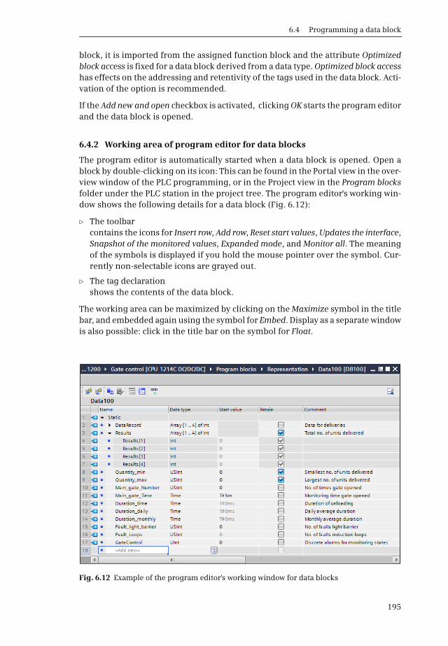
6.4 Programming a data block
195
block, it is imported from the assigned function block and the attribute Optimizedblock access is fixed for a data block derived from a data type. Optimized block accesshas effects on the addressing and retentivity of the tags used in the data block. Acti-vation of the option is recommended.
If the Add new and open checkbox is activated, clicking OK starts the program editorand the data block is opened.
6.4.2 Working area of program editor for data blocks
The program editor is automatically started when a data block is opened. Open ablock by double-clicking on its icon: This can be found in the Portal view in the over-view window of the PLC programming, or in the Project view in the Program blocksfolder under the PLC station in the project tree. The program editor's working win-dow shows the following details for a data block (Fig. 6.12):
b The toolbarcontains the icons for Insert row, Add row, Reset start values, Updates the interface,Snapshot of the monitored values, Expanded mode, and Monitor all. The meaningof the symbols is displayed if you hold the mouse pointer over the symbol. Cur-rently non-selectable icons are grayed out.
b The tag declarationshows the contents of the data block.
The working area can be maximized by clicking on the Maximize symbol in the titlebar, and embedded again using the symbol for Embed. Display as a separate windowis also possible: click in the title bar on the symbol for Float.
Fig. 6.12 Example of the program editor's working window for data blocks

6 Program editor
196
You can save the structure of the windows and tables using the Save windows set-tings icon in the top right corner of the working window. This structure is reestab-lished the next time the working window is opened.
6.4.3 Defining properties for data blocks
To set the block properties, select the block in the Program blocks folder, followedby the Edit > Properties command in the main menu or the Properties command inthe shortcut menu. The block properties that can be changed are described in detailin Chapter 5.3.2 “Editing block properties” on page 128. A data block can be pro-tected against illegal access (“know-how protection”) or illegal use (“copy protec-tion”). You can only set the Optimized block access attribute for a global data blockwhen creating a block; afterwards, it can no longer be changed.
6.4.4 Declaring data tags
The declaration table shows the following columns depending on the block proper-ties and the editing environment:
b Name: The name can contain letters, digits, and special characters (but not quo-tation marks). No distinction is made between upper and lower case when check-ing the name. The name is block-local, and therefore the name can also be usedin other blocks for different tags. In association with the data block whose nameapplies throughout the CPU (“globally”), a data tag becomes a “global” tag appli-cable throughout the CPU.
b Data type: Select the data type of the tag from a drop-down list, or enter itdirectly.
b Offset: The offset indicates the relative address of the tag with respect to the startof the data block or the start of a data structure. The column is only shown if theOptimized block access attribute is not activated in the data block. The offset isshown after the data block has been compiled.
b Default value: The default value is the value which is automatically assigned to anew tag depending on the data type. Example: With the data type DATE, thedefault value is DATE#1990-01-01. If the data block is based on a data type (typedata block) or a function block (instance data block), the tag value defined in thedata type or in the function block is present in the Default value column.
b Start value: The Start value column lists the individual default values of the tagsfor this data block. The default value is used if a start value is not entered. Thestart value is the value with which the data block is loaded into the CPU's workmemory. With an instance data block, it is then possible to commence each call(each instance) with different start values.
b Snapshot: The Snapshot column shows the “frozen” monitoring values fromthe work memory at the time of the snapshot.
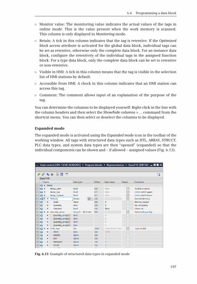
6.4 Programming a data block
197
b Monitor value: The monitoring value indicates the actual values of the tags inonline mode. This is the value present when the work memory is scanned.This column is only displayed in Monitoring mode.
b Retain: A tick in this column indicates that the tag is retentive. If the Optimizedblock access attribute is activated for the global data block, individual tags canbe set as retentive, otherwise only the complete data block. For an instance datablock, configure the retentivity of the individual tags in the assigned functionblock. For a type data block, only the complete data block can be set to retentiveor non-retentive.
b Visible in HMI: A tick in this column means that the tag is visible in the selectionlist of HMI stations by default.
b Accessible from HMI: A check in this column indicates that an HMI station canaccess this tag.
b Comment: The comment allows input of an explanation of the purpose of thetag.
You can determine the columns to be displayed yourself: Right-click in the line withthe column headers and then select the Show/hide columns > ... command from theshortcut menu. You can then select or deselect the columns to be displayed.
Expanded mode
The expanded mode is activated using the Expanded mode icon in the toolbar of theworking window. All tags with structured data types such as DTL, ARRAY, STRUCT,PLC data types, and system data types are then “opened” (expanded) so that theindividual components can be shown and – if allowed – assigned values (Fig. 6.13).
Fig. 6.13 Example of structured data types in expanded mode
6 Program editor
198
6.4.5 Entering data tags in global data blocks
With a global data block, you enter the data tags directly in the block. In the Namecolumn you specify the name of the tag. Following input of the name, select the datatype from a drop-down list, enter a start value if applicable, and use a comment toexplain the purpose of the tag.
With the STRING data type, enter the maximum length of the string in square brack-ets. If this data is missing, the standard length of 254 characters is used.
With the ARRAY data type, you must enter the range limits and the component datatype. For example, the information in the drop-down list Array [lo .. hi] of type couldthen result in Array [1 .. 12] of Real. If you click on the triangle to the left of the tagname, the components are displayed, and you can assign individual start values tothem as default values.
Select the STRUCT data type from the drop-down list and, in the line under the tagname, enter the name of the first component, its data type, possibly a default set-ting, and a comment. The next line contains the second component, etc.
When programming a tag with PLC data type, select the PLC data type from thedrop-down list. If you click on the triangle to the left of the tag name, the compo-nents are displayed, and you can assign individual start values to them as defaultvalues.
When programming a tag with a system data type whose structure is defined bySTEP 7, such as ErrorStruct or IEC_TIMER, you cannot change the structure and canonly carry out a default setting for individual components where permissible.
6.5 Compiling blocks
Compilation generates a program code which can execute in the CPU. A compila-tion process is always triggered prior to downloading the user program to the PLCstation. Only blocks which have been compiled without errors can be downloaded.
It is recommendable to also trigger compilation while generating the user programto enable a quick response to any programming errors.
6.5.1 Starting the compilation
You start the compilation using a command from the shortcut menu.
b To compile a block opened in the program editor, click with the right mouse but-ton on the white background of the working area and select the Compile com-mand.
b To compile a block listed in the call structure or in the dependency structure,click with the right mouse button on the block and select the Compile command.
b To start the compilation process for the selected block, click with the right mousebutton on the block in the Program blocks folder in the project tree followed bythe Compile > Software command.

6.5 Compiling blocks
199
b You can also select several blocks in the Program blocks folder and compile themtogether using the Compile > Software command from the shortcut menu.
b You can compile the entire user program by selecting the Program blocks folderfollowed by Compile > … from the shortcut menu. You then have the choicebetween … Software (compile program changes since last compilation only) and… Software (rebuild all blocks) (compilation of entire program).
b If you select the PLC station folder and then Compile > … from the shortcut menu,you can select between
– … All (complete compilation of all project information relevant to execution)
– … Hardware configuration (compilation of device and network configuration)
– … Software (compilation of program changes since last compilation only) and
– … Software (rebuild all blocks) (compilation of entire user program)
The result of the compilation is displayed in the inspector window in the Info tabunder Compile (Fig. 6.14). Any warnings which have been detected do not preventcontinuation of the compilation. Any errors which have been detected are displayedin the result of the compilation, and end the compilation.
6.5.2 Compiling SCL blocks
You can set the attributes for compilation in the properties of SCL blocks. The set-ting for all newly created blocks is specified in the main menu under Options > Set-tings and PLC programming > SCL > Compile.
The activatable attributes are:
b Create extended status informationpermits monitoring of all tags in a block.
Fig. 6.14 Example of compilation information in the inspector window
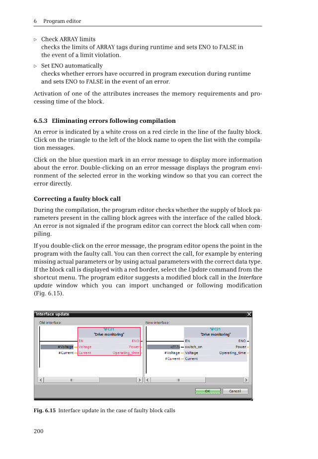
6 Program editor
200
b Check ARRAY limitschecks the limits of ARRAY tags during runtime and sets ENO to FALSE in the event of a limit violation.
b Set ENO automaticallychecks whether errors have occurred in program execution during runtime and sets ENO to FALSE in the event of an error.
Activation of one of the attributes increases the memory requirements and pro-cessing time of the block.
6.5.3 Eliminating errors following compilation
An error is indicated by a white cross on a red circle in the line of the faulty block.Click on the triangle to the left of the block name to open the list with the compila-tion messages.
Click on the blue question mark in an error message to display more informationabout the error. Double-clicking on an error message displays the program envi-ronment of the selected error in the working window so that you can correct theerror directly.
Correcting a faulty block call
During the compilation, the program editor checks whether the supply of block pa-rameters present in the calling block agrees with the interface of the called block.An error is not signaled if the program editor can correct the block call when com-piling.
If you double-click on the error message, the program editor opens the point in theprogram with the faulty call. You can then correct the call, for example by enteringmissing actual parameters or by using actual parameters with the correct data type.If the block call is displayed with a red border, select the Update command from theshortcut menu. The program editor suggests a modified block call in the Interfaceupdate window which you can import unchanged or following modification(Fig. 6.15).
Fig. 6.15 Interface update in the case of faulty block calls
6.6 Program information
201
Not all block parameters have to be supplied for a function block call. If such a blockparameter is added subsequently, the compilation does not signal an error – thesupply simply remains open. Even if the assignment of the static local data ischanged, a new instance data block is generated during the compilation, and an er-ror message is not produced. If the instance data block for compilation is missing,a new data block with the next free number is simply generated, also without an er-ror message.
Under Options > Settings and PLC programming > General > Compilation, you canselect the option Delete actual parameters on interface update. The result is that anactual parameter is deleted when compiling or updating the interface if the associ-ated block parameter has been deleted. An error message is then not output.
How you can nevertheless find the call of a block with a subsequently modified in-terface in the program is shown in Section 6.6.5 “Consistency check” on page 206.
6.6 Program information
The following program information supports you during programming and pro-gram debugging:
b Cross-references
b Assignment list (inputs, outputs and bit memories)
b Call and dependency structures
b Resources
You can start the individual tools at any time during program creation, either in themain menu using the Tools > … command or in the project tree by double-clickingProgram info under a PLC station. Following commissioning, the program informa-tion can be part of the project documentation.
6.6.1 Cross-reference list
The cross-reference list indicates the use of tags, hardware constants, and blocks inthe user program. It provides an overview of
b Which objects have been used
b At which position in the program they have been used, and
b the context in which they were used, e.g. whether there is read or write access to a tag .
You can create cross-references from any data object of a station: select the station,a folder under the station, or one or more objects in a folder, e.g. one or moreblocks or PLC tags, and then select the Cross-reference list command from the short-cut menu or the Tools > Cross-references command from the main menu. The cross-reference list is available in two views: Used by and Uses.
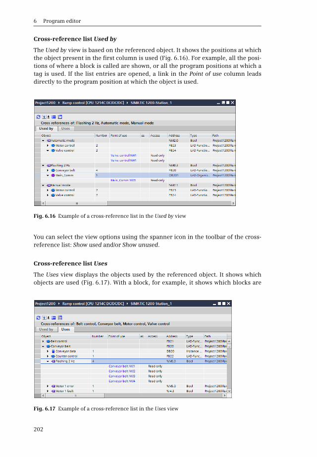
6 Program editor
202
Cross-reference list Used by
The Used by view is based on the referenced object. It shows the positions at whichthe object present in the first column is used (Fig. 6.16). For example, all the posi-tions of where a block is called are shown, or all the program positions at which atag is used. If the list entries are opened, a link in the Point of use column leadsdirectly to the program position at which the object is used.
You can select the view options using the spanner icon in the toolbar of the cross-reference list: Show used and/or Show unused.
Cross-reference list Uses
The Uses view displays the objects used by the referenced object. It shows whichobjects are used (Fig. 6.17). With a block, for example, it shows which blocks are
Fig. 6.16 Example of a cross-reference list in the Used by view
Fig. 6.17 Example of a cross-reference list in the Uses view

6.6 Program information
203
called within it and which tags are used within it. If the list entries are opened, a linkin the Location column leads directly to the program position at which the associ-ated object is used.
You can select the view options using the spanner icon in the toolbar of the cross-reference list: Show defined and/or Show not undefined.
Display of cross-references in the inspector window
Select an object, e.g. a block in the project tree or a tag in the working window, andthen select the Cross-reference information command in the shortcut menu. Theinspector window – under Cross-references in the Info tab – shows the program posi-tions at which the selected object has been used. If the cross-reference list is openin the inspector window, the use of the selected object is displayed directly.
6.6.2 Assignment list
The assignment list shows the assignment of the operand areas: inputs (I), outputs(Q) and bit memories (M). Peripheral inputs (I:P) which are used are shown underthe input address, peripheral outputs (Q:P) which are used are shown under theoutput address. The use of operands as bit, byte, word or doubleword operands ortags is displayed.
You can display the assignment list for individual blocks or for the entire program:Select the blocks, the Program blocks folder or the folder of the PLC station, andthen select Assignment list from the shortcut menu or Tools > Assignment list in themain menu (Fig. 6.18).
Fig. 6.18 Example of an assignment list
6 Program editor
204
Display of input/output assignment
A yellow background for inputs and outputs indicates that the address is not usedby the hardware or that no hardware has been configured for this address. If youadditionally address a bit in a byte, word or double word operand, the entry has agray background. You can use the View options symbol in the toolbar of the assign-ment list to select whether the used addresses and/or the free hardware addressesare to be displayed.
Display of bit memory assignment
The view option must be set to Used addresses in order to display the bit memoryassignment. With the bit memories, symbols are used for the operands to indicatethose which are set as clock and system memories, and up to which address the bitmemories are retentive. You can switch the retentivity display on and off using thecorresponding symbol in the toolbar. You can set the retentive range for the bitmemories using the Retain symbol.
Filter
You can filter the display of the assignment list using the Filter symbol in the tool-bar. You specify which addresses (operands) you wish to view: to select the operandarea, activate the associated check box. You can select all addresses as the filter area(with an asterisk: *), a section of the address area using a hyphen (e.g. 0-100),an individual address (e.g. 101), or several areas separated by a semicolon (e.g. 0-100; 120-124; 160).
If you wish to repeatedly use the particular settings of a filter, assign a name to it inthe drop-down list of the filter dialog. You can then use this name to recall the filtersettings from the drop-down list in the toolbar of the assignment list. You can alsodelete filter names again.
6.6.3 Call structure
The call structure describes the call hierarchy of the blocks. To display the call struc-ture, select the PLC station or Program blocks folder for the entire program or forindividual blocks and then select Call structure from the shortcut menu or Tools >Call structure from the main menu.
The call structure shows the used blocks and the logic blocks called from theseblocks or the data blocks used in them (Fig. 6.19). The blocks that are not called inthe user program are present in the first level (color highlighted) – in the finishedprogram, these should only be the organization blocks.
Starting with the call structure, you can display the cross-reference information oropen a block for processing with the program editor. The consistency test for theblock calls is described in Chapter 6.6.5 “Consistency check” on page 206.
You can set the view options using the View options icon in the toolbar: Show con-flicts only then displays the call paths in which conflicts have been detected, e.g.

6.6 Program information
205
interface conflicts, recursive calls, or non-existent block calls. Group multiple callstogether displays several calls of a block or data block access operations in a singleline, and specifies the number of calls in a separate column.
For compiled blocks, the memory requirements for temporary local data of a blockand in the path are displayed.
6.6.4 Dependency structure
The dependency structure shows the dependencies of each block. To display thedependency structure, first select the PLC station or Program blocks folder for theentire program or for individual blocks, and then select Tools > Dependency struc-ture from the main menu.
For each logic block the dependency structure shows the block from which it iscalled, and for each data block the logic block in which it is used (Fig. 6.20).
From the dependency structure, you can display the cross-reference information oropen a block for processing with the program editor. The consistency test for theblock calls is described in the next Chapter 6.6.5 “Consistency check”.
You can set the view options using the View options icon in the toolbar: Show con-flicts only then displays the call paths in which conflicts have been detected, e.g.interface conflicts, recursive calls, or non-existent block calls. Group multiple callstogether displays several calls of a block or data block access operations in a singleline, and specifies the number of calls in a separate column.
Fig. 6.19 Example of call structure

6 Program editor
206
6.6.5 Consistency check
Clicking on the Consistency check icon in the toolbar of the call structure or depen-dency structure displays block calls with an “interface conflict”. These are blockcalls whose interface is subsequently changed, such as by assigning another datatype to a block parameter or by adding a block parameter.
Blocks which have not yet been compiled following a modification are displayedwith a red border. In order to compile individual blocks in the call or dependencystructure, select Compile in the shortcut menu.
If interface conflicts cannot be eliminated by a repeated compilation, they must behandled manually. The link in the Details column leads to the faulty block call.
Open the calling block, select the block call identified as faulty, and select theUpdate command from the shortcut menu. When updating the block call, the pro-gram editor shows what the updated block call will look like in the Interface updatewindow (for an example, see Fig. 6.15 on page 200). You can then carry out correc-tions and supplements in this window, for example if a new block parameter hasbeen added.
6.6.6 CPU resources
Resources shows the assignment of the user memory and of the existing input/out-put modules. To display resources, first select the PLC station, Program blocks folderor individual blocks, and then select the Resources command from the shortcutmenu or Tools > Resources from the main menu.
Fig. 6.20 Example of dependency structure
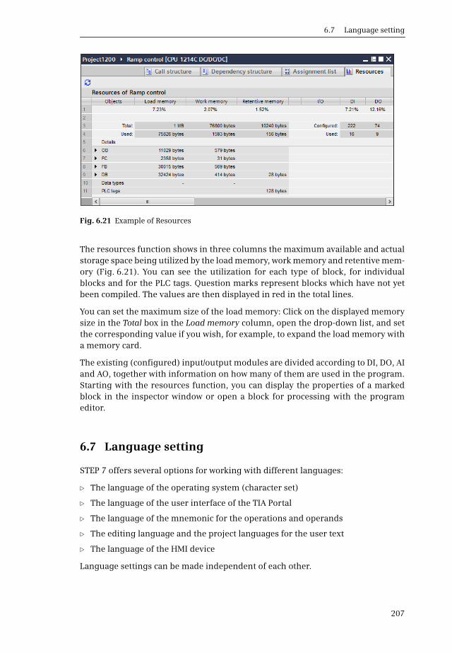
6.7 Language setting
207
The resources function shows in three columns the maximum available and actualstorage space being utilized by the load memory, work memory and retentive mem-ory (Fig. 6.21). You can see the utilization for each type of block, for individualblocks and for the PLC tags. Question marks represent blocks which have not yetbeen compiled. The values are then displayed in red in the total lines.
You can set the maximum size of the load memory: Click on the displayed memorysize in the Total box in the Load memory column, open the drop-down list, and setthe corresponding value if you wish, for example, to expand the load memory witha memory card.
The existing (configured) input/output modules are divided according to DI, DO, AIand AO, together with information on how many of them are used in the program.Starting with the resources function, you can display the properties of a markedblock in the inspector window or open a block for processing with the programeditor.
6.7 Language setting
STEP 7 offers several options for working with different languages:
b The language of the operating system (character set)
b The language of the user interface of the TIA Portal
b The language of the mnemonic for the operations and operands
b The editing language and the project languages for the user text
b The language of the HMI device
Language settings can be made independent of each other.
Fig. 6.21 Example of Resources

6 Program editor
208
Language settings in the operating system
If you are working with a multilingual version of the operating system (MUI ver-sion), set the desired character set using the Windows Control Panel.
The language of the user interface and mnemonic
STEP 7 Basic is operated with the language of the user interface. This comprises, forexample, the menu names and the error messages of the TIA Portal. You can set thislanguage in the Project view in the main menu using Options > Settings in the Gen-eral section. The languages installed with STEP 7 are offered for selection underUser interface language. You also set the programming mnemonics in this tab,i.e. the language in which the program editor uses the operands and operations.For example, with the German setting, “E” stands for “Eingang”, and with the Inter-national setting, “I” stands for “Input”.
Editing language
The user texts are entered in the editing language. These are, for example, com-ments on PLC tags or the program. The editing language is independent of the lan-guage of the user interface. You select the editing language in the project treeunder Languages & Resources > Project languages from the Editing language drop-down list.
Project languages
The text entered in the editing language can be translated into various project lan-guages and displayed. You specify the available project languages in the project treeunder Languages & Resources > Project languages. All entered user texts can befound in the project tree under Languages & Resources > Project texts in the Usertexts tab. The entered texts in of the editing language and the selected project lan-guages are shown. You can enter text directly or edit it here. The displayed texts areoriented on a reference language that you specify under Languages & Resources >Project languages in the Reference languages drop-down list. You can also export thetexts for translation and reimport the translated texts.
To display the translated user texts in configuration and programming, select thedesired project language as editing language.
Language of the HMI station (HMI project language)
The HMI station can be provided with a multilingual user interface. You set the lan-guages available at runtime in the project tree under the HMI station and Runtimesettings. The project languages set under Languages & Resources > Project lan-guages can be selected.
If during runtime you wish to switch over to another language available on the HMIstation, an operator-accessible object, e.g. a button, must have been linked to thelanguage switchover during configuration. Following selection, the new languageis applied immediately. When the HMI station is switched on, the language that wasactive last is always set.

7.1 Introduction
209
7 Ladder logic LAD
7.1 Introduction
This chapter describes programming with ladder logic (LAD); it uses examples toshow how the program functions are represented in LAD. You can find a descriptionof the individual functions, e.g. comparison functions, in Chapter 10 “Basic func-tions” on page 328.
Use of the program and symbol editor, which generally applies to all programminglanguages, is described in Chapter 6 “Program editor” on page 178.
LAD is used to program the contents of blocks (the user program). What blocks are,and how they are created, is described in Chapters 5.3 “Programming blocks” onpage 125 and 6.3 “Programming a code block” on page 183.
7.1.1 Programming with LAD in general
You use LAD to program the control function of the programmable controller – theuser program or control program. The user program is organized in different typesof blocks. A block is divided into sections referred to as “networks”. Each networkcontains at least one current path that may also have an extremely complex struc-ture. Each network is terminated by at least one coil or box.
Fig. 7.1 shows the structure of a block with the LAD program. Located at the begin-ning of the program is the block title, comprising the block heading and block com-ment. Heading and comment are optional. These are followed by the first networkwith its number, heading, and comment. Heading and comment are also optionalfor the networks. The first network shows a current path as an example with seriesand parallel connection of contacts, a memory function within the current path,and two coils as termination of the current path. The second network shows theprocessing of boxes, which can be arranged in series or parallel. A block is not ter-minated by a special network or function, you simply finish the program input.
The LAD editor establishes a network in accordance with the principle of the“main current path”: this is the highest branch which commences directly on theleft-hand power rail and must be terminated by a coil or box. All LAD elements canbe positioned within it.
An LAD element must not be “short-circuited” by an “empty” parallel branch, and“current” must not flow from right to left through a program element. A parallelbranch which does not end “open” must be closed for the branch on which it wasopened.
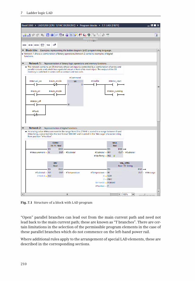
7 Ladder logic LAD
210
“Open” parallel branches can lead out from the main current path and need notlead back to the main current path; these are known as “T branches”. There are cer-tain limitations in the selection of the permissible program elements in the case ofthese parallel branches which do not commence on the left-hand power rail.
Where additional rules apply to the arrangement of special LAD elements, these aredescribed in the corresponding sections.
Fig. 7.1 Structure of a block with LAD program
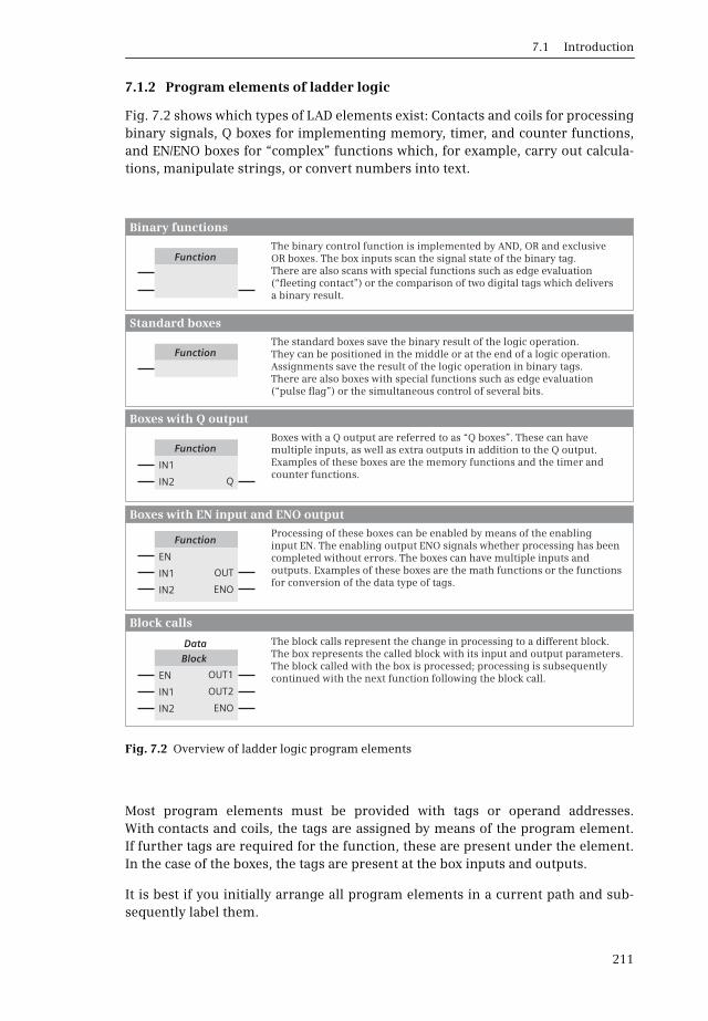
7.1 Introduction
211
7.1.2 Program elements of ladder logic
Fig. 7.2 shows which types of LAD elements exist: Contacts and coils for processingbinary signals, Q boxes for implementing memory, timer, and counter functions,and EN/ENO boxes for “complex” functions which, for example, carry out calcula-tions, manipulate strings, or convert numbers into text.
Most program elements must be provided with tags or operand addresses.With contacts and coils, the tags are assigned by means of the program element.If further tags are required for the function, these are present under the element.In the case of the boxes, the tags are present at the box inputs and outputs.
It is best if you initially arrange all program elements in a current path and sub-sequently label them.
Fig. 7.2 Overview of ladder logic program elements
The binary control function is implemented by AND, OR and exclusive OR boxes. The box inputs scan the signal state of the binary tag. There are also scans with special functions such as edge evaluation (“fleeting contact”) or the comparison of two digital tags which delivers a binary result.
The standard boxes save the binary result of the logic operation. They can be positioned in the middle or at the end of a logic operation. Assignments save the result of the logic operation in binary tags. There are also boxes with special functions such as edge evaluation (“pulse flag”) or the simultaneous control of several bits.
Boxes with a Q output are referred to as “Q boxes”. These can have multiple inputs, as well as extra outputs in addition to the Q output. Examples of these boxes are the memory functions and the timer and counter functions.
Processing of these boxes can be enabled by means of the enabling input EN. The enabling output ENO signals whether processing has been completed without errors. The boxes can have multiple inputs and outputs. Examples of these boxes are the math functions or the functions for conversion of the data type of tags.
The block calls represent the change in processing to a different block. The box represents the called block with its input and output parameters. The block called with the box is processed; processing is subsequently continued with the next function following the block call.
Function
Function
Function
Function
Block
Q
OUT
OUT1
ENO
OUT2
ENO
IN1
EN
EN
IN2
IN2
IN2
IN1
IN1
Data
Binary functions
Standard boxes
Boxes with Q output
Boxes with EN input and ENO output
Block calls

7 Ladder logic LAD
212
7.2 Programming with contacts
In the case of contacts you scan the binary tags, e. g. inputs, and link the scannedsignal states by arranging the contacts in series or parallel. You use an NO or NCcontact to define the influence of the scanned signal state on the logic operation.Further functions for contacts are negation of the signal flow, edge evaluation for abinary tag, validity checking of floating-point numbers, and the comparison func-tion (Fig. 7.3).
7.2.1 NO and NC contacts
An NO or NC contact is used to scan the signal state of a binary tag. An NO contactpasses on the scanned signal state directly to the logic operation, an NC contact firstnegates the signal state.
Normally open contact
If the signal state of a binary tag is scanned using an NO contact, the scanned statedirectly influences the signal flow in the logic operation.
The example in Fig. 7.4 shows the sensor S1 on the left-hand side which is connect-ed to input %I1.0 and is scanned by means of an NO contact. If the sensor S1 is open,the input %I1.0 has the signal state “0” and and no current flows through theNO contact. Contactor K1 controlled by output %Q4.0 does not pull up.
If sensor S1 is then activated, input %I1.0 has the signal state “1”. Current flowsfrom the left-hand power rail through the NO contact into the coil, and contactor K1connected to output %Q4.0 pulls up.
Fig. 7.3 Overview of contacts available with LAD
Normally open (NO) contact
NOT contact
Normally closed (NC) contact
Scan for “valid”
Comparison function
Scan for “invalid”
NOT
Floating-point tag Floating-point tagOK NOT_OK
Binary tag Binary tagP N
Edge trigger flag Edge trigger flag
FunctionData type
Digital tag 1
Digital tag 2
Contacts
Positive edge of a binary tag
Binary tag Binary tag
Negative edge of a binary tag

7.2 Programming with contacts
213
Normally closed contact
If the signal state of a binary tag is scanned using an NC contact, the contact passeson the negated result of the scan to the signal flow in the logic operation.
In the example in Fig. 7.4 (right-hand side), current flows through the NC contactif the scanned sensor S2 is not closed (input %I1.1 has the signal state “0”).The current also flows into the coil and triggers the contactor K2 at output %Q4.1.
If sensor S2 is then activated, “1” is present at the input %I1.1 and the NC contactopens. The current flow is interrupted, and contactor K2 drops out.
7.2.2 Consideration of sensor type in ladder logic
If you scan a sensor in your program, you must take into consideration whether itis an NO or NC contact. Depending on the type of sensor, different signal states arepresent at the corresponding input when the sensor is activated: “1” with an NOcontact and “0” with an NC contact. It is not possible for the CPU to determinewhether an NC or NO contact is connected to an input. It can only recognize the sig-nal state “1” or “0”.
Fig. 7.4 Principle of operation of NO and NC contacts
S1 S2
C1 C2C1 C2
S1 S2
%I1.0 %I1. 1%Q4.0 %Q4.1%Q4.0 %Q4.1%I1. 0 %I1.1
“0”
“1”“1”
“1”“1”
“0”“0”
“0”
Principle of operation of a NC contact Principle of operation of a NO contact
Sensor activated
Sensor activated
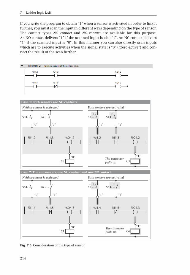
7 Ladder logic LAD
214
If you write the program to obtain “1” when a sensor is activated in order to link itfurther, you must scan the input in different ways depending on the type of sensor.The contact types NO contact and NC contact are available for this purpose.An NO contact delivers “1” if the scanned input is also “1”. An NC contact delivers“1” if the scanned input is “0”. In this manner you can also directly scan inputswhich are to execute activities when the signal state is “0” (“zero-active”) and con-nect the result of the scan further.
Fig. 7.5 Consideration of the type of sensor
Neither sensor is activated
Neither sensor is activated
Both sensors are activated
Both sensors are activated
The contactor pulls up
The contactor pulls up
S3
S5
S3
S5
S4
S6
S4
S6
C3
C4
C3
C4
%I1.2
%I1.4
%I1.2
%I1.4
%I1.3
%I1.5
%I1.3
%I1.5
%Q4.2
%Q4.3
%Q4.2
%Q4.3
“0”
“0”
“0” “1”
“1”
“1”
“1”“1”
“1”
“1”
“0”
“0”
Case 1: Both sensors are NO contacts
Case 2: The sensors are one NO contact and one NC contact

7.2 Programming with contacts
215
The example in Fig. 7.5 on page 214 shows the programming dependent on thetype of sensor. In the first case, two NO contacts are connected to the programmablecontroller, in the second case one NO contact and one NC contact. In both cases, acontactor connected to an output is to pull up when both sensors are activated.When an NO contactor is activated, the signal state at the input is “1” and is scannedby an NO contact so that current can flow when the sensor is activated. If both NOcontacts are activated, current flows through the current path into the coil, and thecontactor pulls up.
When activating an NC contact, the signal state at the input is “0”. To allow currentto flow following activation, an NC contact must be used for the scan. Therefore inthe second case one NO contact and one NC contact must be connected in series inorder for the contactor to pull up when both sensors are activated.
7.2.3 Series connection of contacts
With a series connection, two or more contacts are positioned one behind the other.Current flows through a series connection when all contacts are closed.
Fig. 7.6 shows an example of a series connection: If in the upper current path alltags have signal state “1”, all NO contacts are closed and the tag “Coil 1” is set to sig-nal state “1”. In all other cases, “Coil 1” is reset to signal state “0”.
In the current path underneath this, the tag “Coil 2” is set to signal state “1” if“Contact 4” has the signal state “1” and “Contact 5” the signal state “0”.
7.2.4 Parallel connection of contacts
A parallel connection means that two or more contacts are positioned underneatheach other. Current flows through a parallel connection when one of the contacts isclosed.
Fig. 7.7 shows an example of a parallel connection: if none of the tags has the signalstate “1” in the top current path, all NO contacts are open and the tag “Coil 3” hasthe signal state “0”. In all other cases, “Coil 3” is set to signal state “1”.
In the current path underneath this, the tag “Coil 4” has the signal state “0” if thetag “Contact 4” has the signal state “0” and the tag “Contact 5” the signal state “1”.
Fig. 7.6 Series connection of contacts

7 Ladder logic LAD
216
With LAD you can also program a branch in the middle of a current path, such asthe top current path in . The result is a parallel branch which does not commenceon the left-hand power rail. A parallel connection with an “open” termination is re-ferred to as a “T branch” (see Chapter 7.2.6 “T branch, open parallel branch in theladder logic” on page 217). In both cases, use of LAD program elements is limited;reference to this is made in the corresponding sections.
7.2.5 Mixed series and parallel connections
You can combine series and parallel connections, e.g. arrange several series con-nections in parallel or several parallel connections in series. You can also connectseries or parallel connections together even if they have a complex structure.
Parallel connection of series connections
Instead of contacts you can also arrange series connections underneath each other.Fig. 7.8 shows two examples. The tag “Coil 5” is set to signal state “1” if “Contact 1”
Fig. 7.7 Parallel connection of contacts
Fig. 7.8 Parallel connection of series connections
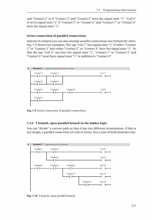
7.2 Programming with contacts
217
and “Contact 2” or if “Contact 3” and “Contact 4” have the signal state “1”. “Coil 6”is set to signal state “1” if “Contact 5” or “Contact 6” and “Contact 7” or “Contact 0”have the signal state “1”.
Series connection of parallel connections
Instead of contacts you can also arrange parallel connections one behind the other.Fig. 7.9 shows two examples. The tag “Coil 7” has signal state “1” if either “Contact1” or “Contact 3” and either “Contact 2” or “Contact 4” have the signal state “1”. Sothat the tag “Coil 0” can have the signal state “1”, “Contact 7” or “Contact 5” and“Contact 6” must have signal state “1” in addition to “Contact 0”.
7.2.6 T branch, open parallel branch in the ladder logic
You can “divide” a current path so that it has two different terminations. If this isnot simply a parallel connection of coils or boxes, but a case of both branches hav-
Fig. 7.9 Series connection of parallel connections
Fig. 7.10 T branch, open parallel branch

7 Ladder logic LAD
218
ing different logic operations, this is referred to as a “T branch” or an “open” paral-lel branch.
Fig. 7.10 shows a simple T branch in the top current path. “Coil 8” can be switchedon by the tag “Contact 2”, and “Coil 9” by the tag “Contact 3”. A prerequisite in bothcases is that the tag “Contact 1” has the signal state “1”.
Series and parallel contact connections can be programmed following a T branch.A further T branch can also be opened within a T branch. However, you cannot enterlogic operations which lead from the left-hand power rail to a T branch.
7.2.7 Negating result of logic operation in the ladder logic
The NOT contact negates the result of the logic operation (the “current flow”). Youcan use this contact to negate the result of a series connection, for example. InFig. 7.11, “Coil 13” only has a signal state “0” if both “Contact 1” and “Contact 2”have the signal state “1”.
In the bottom current path, a NOT contact is positioned following a parallel connec-tion. In this case, “Coil 14” is only set to signal state “1” if both tags “Contact 3” and“Contact 4” have the signal state “0”.
You can position the NOT contact like a standard contact in a branch which com-mences on the left-hand power rail. Positioning following a T branch is also permis-sible. Positioning of the NOT contact is not permissible in a parallel branch whichcommences in the middle of the current path. The NOT contact can also be used tonegate the result of the logic operation (the “current flow”) at box inputs andoutputs.
7.2.8 Edge evaluation of a binary tag in ladder logic
The edge contact has the signal state “1” for one processing cycle if the signal stateof the binary tags positioned above it changes from “0” to “1” (P contact, risingedge) or from “1” to “0” (N contact, falling edge). It responds like a “fleeting con-tact”. This “pulse” is linked to the result of the logic operation present prior to thecontact.
Fig. 7.11 Example of NOT contact
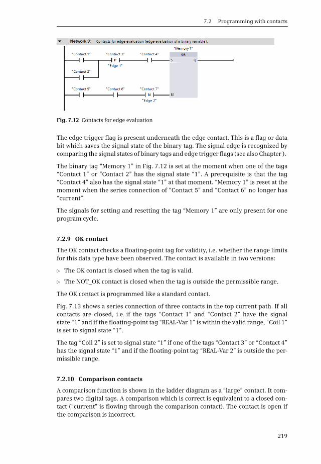
7.2 Programming with contacts
219
The edge trigger flag is present underneath the edge contact. This is a flag or databit which saves the signal state of the binary tag. The signal edge is recognized bycomparing the signal states of binary tags and edge trigger flags (see also Chapter ).
The binary tag “Memory 1” in Fig. 7.12 is set at the moment when one of the tags“Contact 1” or “Contact 2” has the signal state “1”. A prerequisite is that the tag“Contact 4” also has the signal state “1” at that moment. “Memory 1” is reset at themoment when the series connection of “Contact 5” and “Contact 6” no longer has“current”.
The signals for setting and resetting the tag “Memory 1” are only present for oneprogram cycle.
7.2.9 OK contact
The OK contact checks a floating-point tag for validity, i.e. whether the range limitsfor this data type have been observed. The contact is available in two versions:
b The OK contact is closed when the tag is valid.
b The NOT_OK contact is closed when the tag is outside the permissible range.
The OK contact is programmed like a standard contact.
Fig. 7.13 shows a series connection of three contacts in the top current path. If allcontacts are closed, i.e. if the tags “Contact 1” and “Contact 2” have the signalstate “1” and if the floating-point tag “REAL-Var 1” is within the valid range, “Coil 1”is set to signal state “1”.
The tag “Coil 2” is set to signal state “1” if one of the tags “Contact 3” or “Contact 4”has the signal state “1” and if the floating-point tag “REAL-Var 2” is outside the per-missible range.
7.2.10 Comparison contacts
A comparison function is shown in the ladder diagram as a “large” contact. It com-pares two digital tags. A comparison which is correct is equivalent to a closed con-tact (“current” is flowing through the comparison contact). The contact is open ifthe comparison is incorrect.
Fig. 7.12 Contacts for edge evaluation

7 Ladder logic LAD
220
Comparison functions are available for equal to, not equal to, greater than, greaterthan or equal to, less than, and less than or equal to. The comparison is carried outin accordance with the data type of the digital tags involved (for description, seeChapter 11.1 “Transfer functions” on page 356).
The comparison contact can be programmed wherever a standard contact can alsobe positioned. If comparison contacts are connected in series, both comparisonsmust be fulfilled so that current flows in the current path. If comparison contactsare connected in parallel, it is sufficient for one of the comparisons to be fulfilled sothat current flows in the parallel connection.
The tag “Coil 3” in Fig. 7.14 is set to signal state “1” if the floating-point tags“REAL-Var 1” and “REAL-Var 2” have the same numerical value. “Coil 4” is set to “1”if the value of “REAL-Var 1” is greater than 125.75 or if the value of “REAL-Var 2” isless than 12.5·103 and if, in both cases, the values of the tags “INT-Var 1” and “INT-Var 2” are not the same.
In addition there is the range comparison which is represented as a box. The box ispositioned like a standard contact in the current path, with the input and outputunnamed.
Fig. 7.13 OK and NOT_OK contacts
Fig. 7.14 Comparison of contacts

7.3 Programming with coils
221
7.3 Programming with coils
Coils control binary tags such as outputs or bit memories. A simple coil sets the bi-nary tag when current flows into the coil, and resets it when current no longerflows. The reverse is true for a negated coil.
There are coils with additional names and special functionalities, such as the setand reset coils or the coils for pulse generation during evaluation of signal edges.Coils can also be used to set and reset bit fields, start and reset timer functions, exe-cute jumps in the program, and to terminate blocks (Fig. 7.15). The jump functionsand the block end function are described in Chapter 7.6 “Functions for programflow control (LAD)” on page 241.
Fig. 7.15 Overview of coils available with LAD
Negated coil
Reset coil
Binary tag
Binary tag
Binary tag
Binary tag
Simple coil
Set coil
Jump with “1”
Conditional block end
Start time
Reset timeSpecify duration
FKT: TP Pulse timeTON ON delayTOF OFF delayTONR Accumulate time
Jump with “0”Jump destination
Binary tag
Jump destinationJMP
RET
JMPN
SET_BF
FKT
RT
RESET_BF
PT
Pulse onpositive edge
Pulse onnegative edge
Binary tag Binary tag
S
P
R
NEdge trigger flag Edge trigger flag
Binary tag
Timer function
Timer function
Binary tag
Timer function
Number
Duration
Number
Duration
Coils
Multiple setting Multiple resetting
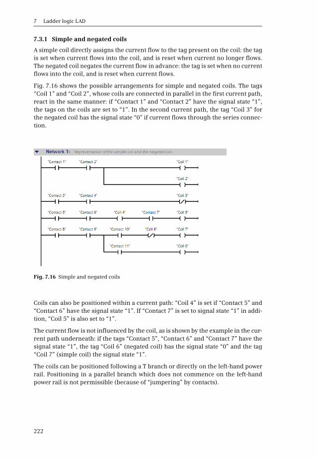
7 Ladder logic LAD
222
7.3.1 Simple and negated coils
A simple coil directly assigns the current flow to the tag present on the coil: the tagis set when current flows into the coil, and is reset when current no longer flows.The negated coil negates the current flow in advance: the tag is set when no currentflows into the coil, and is reset when current flows.
Fig. 7.16 shows the possible arrangements for simple and negated coils. The tags“Coil 1” and “Coil 2”, whose coils are connected in parallel in the first current path,react in the same manner: if “Contact 1” and “Contact 2” have the signal state “1”,the tags on the coils are set to “1”. In the second current path, the tag “Coil 3” forthe negated coil has the signal state “0” if current flows through the series connec-tion.
Coils can also be positioned within a current path: “Coil 4” is set if “Contact 5” and“Contact 6” have the signal state “1”. If “Contact 7” is set to signal state “1” in addi-tion, “Coil 5” is also set to “1”.
The current flow is not influenced by the coil, as is shown by the example in the cur-rent path underneath: if the tags “Contact 5”, “Contact 6” and “Contact 7” have thesignal state “1”, the tag “Coil 6” (negated coil) has the signal state “0” and the tag“Coil 7” (simple coil) the signal state “1”.
The coils can be positioned following a T branch or directly on the left-hand powerrail. Positioning in a parallel branch which does not commence on the left-handpower rail is not permissible (because of “jumpering” by contacts).
Fig. 7.16 Simple and negated coils
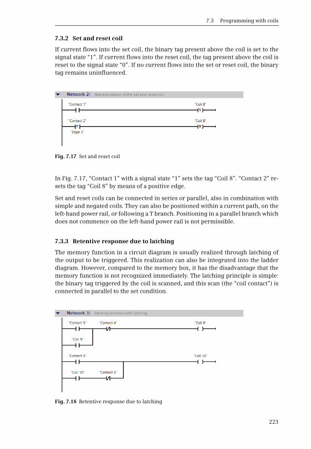
7.3 Programming with coils
223
7.3.2 Set and reset coil
If current flows into the set coil, the binary tag present above the coil is set to thesignal state “1”. If current flows into the reset coil, the tag present above the coil isreset to the signal state “0”. If no current flows into the set or reset coil, the binarytag remains uninfluenced.
In Fig. 7.17, “Contact 1” with a signal state “1” sets the tag “Coil 8”. “Contact 2” re-sets the tag “Coil 8” by means of a positive edge.
Set and reset coils can be connected in series or parallel, also in combination withsimple and negated coils. They can also be positioned within a current path, on theleft-hand power rail, or following a T branch. Positioning in a parallel branch whichdoes not commence on the left-hand power rail is not permissible.
7.3.3 Retentive response due to latching
The memory function in a circuit diagram is usually realized through latching ofthe output to be triggered. This realization can also be integrated into the ladderdiagram. However, compared to the memory box, it has the disadvantage that thememory function is not recognized immediately. The latching principle is simple:the binary tag triggered by the coil is scanned, and this scan (the “coil contact”) isconnected in parallel to the set condition.
Fig. 7.17 Set and reset coil
Fig. 7.18 Retentive response due to latching
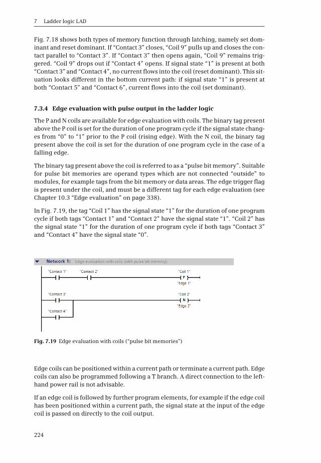
7 Ladder logic LAD
224
Fig. 7.18 shows both types of memory function through latching, namely set dom-inant and reset dominant. If “Contact 3” closes, “Coil 9” pulls up and closes the con-tact parallel to “Contact 3”. If “Contact 3” then opens again, “Coil 9” remains trig-gered. “Coil 9” drops out if “Contact 4” opens. If signal state “1” is present at both“Contact 3” and “Contact 4”, no current flows into the coil (reset dominant). This sit-uation looks different in the bottom current path: if signal state “1” is present atboth “Contact 5” and “Contact 6”, current flows into the coil (set dominant).
7.3.4 Edge evaluation with pulse output in the ladder logic
The P and N coils are available for edge evaluation with coils. The binary tag presentabove the P coil is set for the duration of one program cycle if the signal state chang-es from “0” to “1” prior to the P coil (rising edge). With the N coil, the binary tagpresent above the coil is set for the duration of one program cycle in the case of afalling edge.
The binary tag present above the coil is referred to as a “pulse bit memory”. Suitablefor pulse bit memories are operand types which are not connected “outside” tomodules, for example tags from the bit memory or data areas. The edge trigger flagis present under the coil, and must be a different tag for each edge evaluation (seeChapter 10.3 “Edge evaluation” on page 338).
In Fig. 7.19, the tag “Coil 1” has the signal state “1” for the duration of one programcycle if both tags “Contact 1” and “Contact 2” have the signal state “1”. “Coil 2” hasthe signal state “1” for the duration of one program cycle if both tags “Contact 3”and “Contact 4” have the signal state “0”.
Edge coils can be positioned within a current path or terminate a current path. Edgecoils can also be programmed following a T branch. A direct connection to the left-hand power rail is not advisable.
If an edge coil is followed by further program elements, for example if the edge coilhas been positioned within a current path, the signal state at the input of the edgecoil is passed on directly to the coil output.
Fig. 7.19 Edge evaluation with coils (“pulse bit memories”)
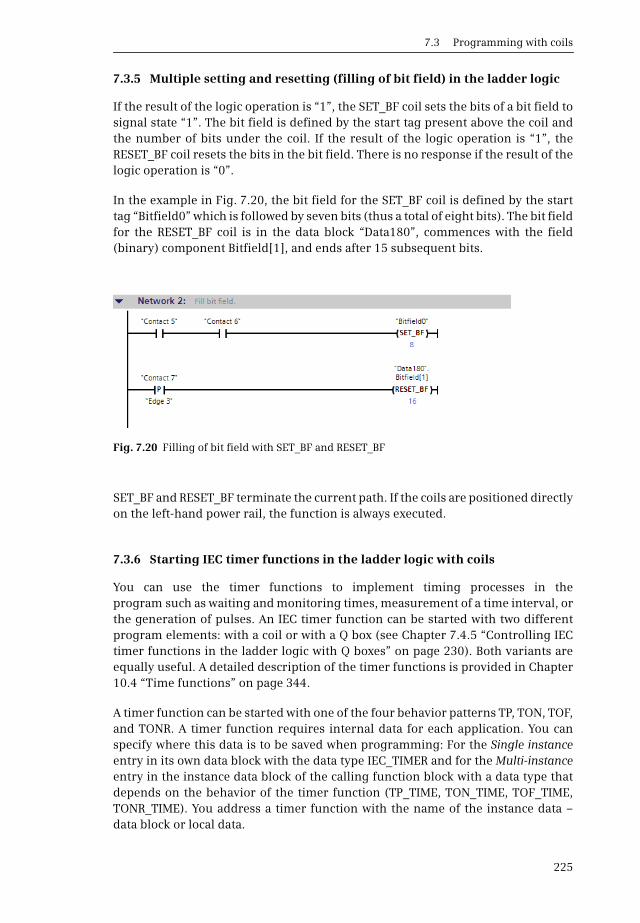
7.3 Programming with coils
225
7.3.5 Multiple setting and resetting (filling of bit field) in the ladder logic
If the result of the logic operation is “1”, the SET_BF coil sets the bits of a bit field tosignal state “1”. The bit field is defined by the start tag present above the coil andthe number of bits under the coil. If the result of the logic operation is “1”, theRESET_BF coil resets the bits in the bit field. There is no response if the result of thelogic operation is “0”.
In the example in Fig. 7.20, the bit field for the SET_BF coil is defined by the starttag “Bitfield0” which is followed by seven bits (thus a total of eight bits). The bit fieldfor the RESET_BF coil is in the data block “Data180”, commences with the field(binary) component Bitfield[1], and ends after 15 subsequent bits.
SET_BF and RESET_BF terminate the current path. If the coils are positioned directlyon the left-hand power rail, the function is always executed.
7.3.6 Starting IEC timer functions in the ladder logic with coils
You can use the timer functions to implement timing processes in theprogram such as waiting and monitoring times, measurement of a time interval, orthe generation of pulses. An IEC timer function can be started with two differentprogram elements: with a coil or with a Q box (see Chapter 7.4.5 “Controlling IECtimer functions in the ladder logic with Q boxes” on page 230). Both variants areequally useful. A detailed description of the timer functions is provided in Chapter10.4 “Time functions” on page 344.
A timer function can be started with one of the four behavior patterns TP, TON, TOF,and TONR. A timer function requires internal data for each application. You canspecify where this data is to be saved when programming: For the Single instanceentry in its own data block with the data type IEC_TIMER and for the Multi-instanceentry in the instance data block of the calling function block with a data type thatdepends on the behavior of the timer function (TP_TIME, TON_TIME, TOF_TIME,TONR_TIME). You address a timer function with the name of the instance data –data block or local data.
Fig. 7.20 Filling of bit field with SET_BF and RESET_BF
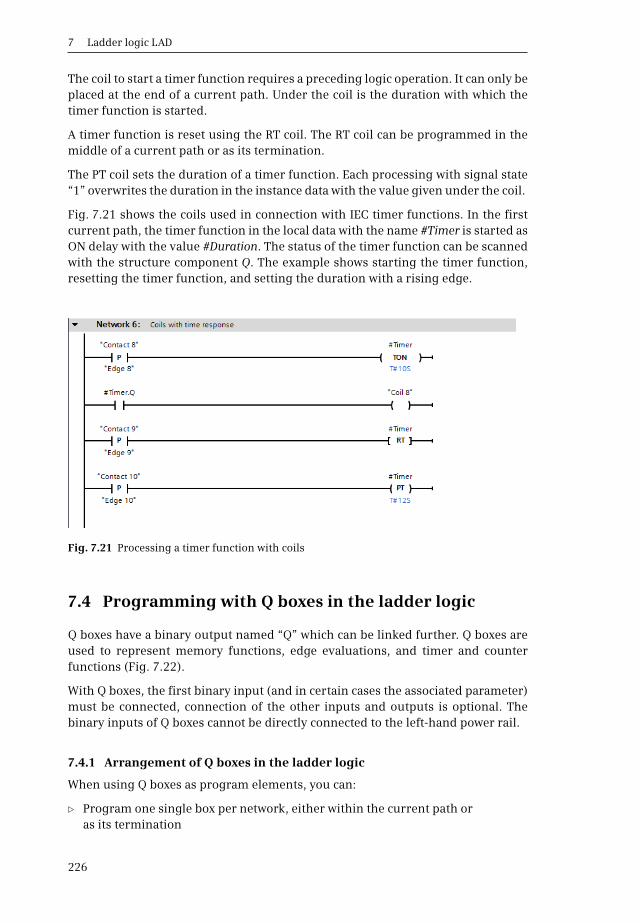
7 Ladder logic LAD
226
The coil to start a timer function requires a preceding logic operation. It can only beplaced at the end of a current path. Under the coil is the duration with which thetimer function is started.
A timer function is reset using the RT coil. The RT coil can be programmed in themiddle of a current path or as its termination.
The PT coil sets the duration of a timer function. Each processing with signal state“1” overwrites the duration in the instance data with the value given under the coil.
Fig. 7.21 shows the coils used in connection with IEC timer functions. In the firstcurrent path, the timer function in the local data with the name #Timer is started asON delay with the value #Duration. The status of the timer function can be scannedwith the structure component Q. The example shows starting the timer function,resetting the timer function, and setting the duration with a rising edge.
7.4 Programming with Q boxes in the ladder logic
Q boxes have a binary output named “Q” which can be linked further. Q boxes areused to represent memory functions, edge evaluations, and timer and counterfunctions (Fig. 7.22).
With Q boxes, the first binary input (and in certain cases the associated parameter)must be connected, connection of the other inputs and outputs is optional. Thebinary inputs of Q boxes cannot be directly connected to the left-hand power rail.
7.4.1 Arrangement of Q boxes in the ladder logic
When using Q boxes as program elements, you can:
b Program one single box per network, either within the current path or as its termination
Fig. 7.21 Processing a timer function with coils

7.4 Programming with Q boxes in the ladder logic
227
b Arrange boxes in series by connecting the Q output of one box to a binary input of the following box, and
b Position boxes following T branches and in branches which commence on the left-hand power rail
The circuits shown in Fig. 7.23 for the positioning of Q boxes use the memory boxwith two binary inputs as an example. This enables the possible positioning of all Qboxes to be shown.
7.4.2 Memory boxes in the ladder logic
There are two versions of the memory function as box: as SR box (reset dominant)and as RS box (set dominant). In addition to the difference in the function name, thetwo boxes also differ in the positioning of the set and reset inputs.
The binary tag named above the memory box is set when the set input has signalstate “1” and the reset input signal state “0”. The binary tag is reset when “1” ispresent at the reset input and “0” at the set input. Signal state “0” at both inputs hasno influence on memory functions. If signal state “1” is present simultaneously atboth inputs, the two memory functions respond differently: the SR memory func-tion is reset, the RS memory function is set.
If both tags “Contact 1” and “Contact 2” in Fig. 7.24 have the same signal state “1”,“Memory 1” is reset (box input R1 is dominant). If both “Contact 3” and “Contact 4”have the same signal state “1”, “Memory 2” is set (box input S1 is dominant).
Fig. 7.22 Overview of Q boxes available with LAD
RS memory boxSR memory box
Evaluation with falling edge
Evaluation with rising edge
Timer functions TP, TON, TOF and TONRCounter functions CTU, CTD, CTUD
Represented as local instance or with own data block
Binary variable Binary variable
SR RS
S R
R1 S1
Q Q
Edge trigger flag Edge trigger flag
P_TRIG N_TRIG
CLK CLKQ Q
FunctionFunction
#Instance
ININ
...
...
...
...
...
...
...
...
“Instance”
Boxes with Q outputs

7 Ladder logic LAD
228
Fig. 7.23 Positioning of Q boxes using example of SR memory function
Fig. 7.24 Memory boxes SR and RS
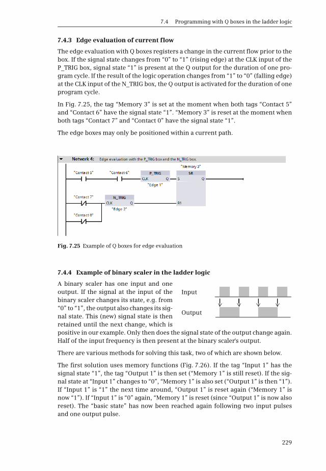
7.4 Programming with Q boxes in the ladder logic
229
7.4.3 Edge evaluation of current flow
The edge evaluation with Q boxes registers a change in the current flow prior to thebox. If the signal state changes from “0” to “1” (rising edge) at the CLK input of theP_TRIG box, signal state “1” is present at the Q output for the duration of one pro-gram cycle. If the result of the logic operation changes from “1” to “0” (falling edge)at the CLK input of the N_TRIG box, the Q output is activated for the duration of oneprogram cycle.
In Fig. 7.25, the tag “Memory 3” is set at the moment when both tags “Contact 5”and “Contact 6” have the signal state “1”. “Memory 3” is reset at the moment whenboth tags “Contact 7” and “Contact 0” have the signal state “1”.
The edge boxes may only be positioned within a current path.
7.4.4 Example of binary scaler in the ladder logic
A binary scaler has one input and oneoutput. If the signal at the input of thebinary scaler changes its state, e.g. from“0” to “1”, the output also changes its sig-nal state. This (new) signal state is thenretained until the next change, which ispositive in our example. Only then does the signal state of the output change again.Half of the input frequency is then present at the binary scaler's output.
There are various methods for solving this task, two of which are shown below.
The first solution uses memory functions (Fig. 7.26). If the tag “Input 1” has thesignal state “1”, the tag “Output 1” is then set (“Memory 1” is still reset). If the sig-nal state at “Input 1” changes to “0”, “Memory 1” is also set (“Output 1” is then “1”).If “Input 1” is “1” the next time around, “Output 1” is reset again (“Memory 1” isnow “1”). If “Input 1” is “0” again, “Memory 1” is reset (since “Output 1” is now alsoreset). The “basic state” has now been reached again following two input pulsesand one output pulse.
Fig. 7.25 Example of Q boxes for edge evaluation
Input
Output

7 Ladder logic LAD
230
The second solution uses the latching principle common to circuit diagrams(Network 4). The operating principle is the same as with the first solution, but thereset condition – as usual with latching – is “zero-active”.
7.4.5 Controlling IEC timer functions in the ladder logic with Q boxes
You can use the timer functions to implement timing processes in theprogram such as waiting and monitoring times, measurement of a time interval, orthe generation of pulses. An IEC timer function can be started with two differentprogram elements: a coil or a Q box (see Chapter 7.3.6 “Starting IEC timer functionsin the ladder logic with coils” on page 225). Both variants are equally useful. A de-tailed description of the timer functions is provided in Chapter 10.4 “Time func-tions” on page 344.
A timer function can be started with one of the four behavior patterns TP, TON, TOF,and TONR. A timer function requires internal data for each application. You canspecify where this data is to be saved when programming: For the Single instanceentry in its own data block with the data type IEC_TIMER and for the Multi-instanceentry in the instance data block of the calling function block with a data type thatdepends on the behavior of the timer function (TP_TIME, TON_TIME, TOF_TIME,
Fig. 7.26 Examples of binary scalers in ladder logic

7.4 Programming with Q boxes in the ladder logic
231
TONR_TIME). You address a timer function with the name of the instance data –data block or local data.
The top timer function “Timer 1” in Fig. 7.27 saves its data as a local instance withthe name #“Timer 1” in the calling function block. This function is started with“Contact 1” and “Duration 1”. The tag “Coil 1” has the signal state “1” for as long asdefined by the tag “Duration 1”.
The bottom timer function “Timer 2” saves its data in a separate data block“Timer 2”. This function is started with “Contact 2” and “Duration 2”. After expiryof the duration, the tag “Coil 2” has signal state “1”.
The name of the local instance (#“Timer 1”) and the name of the data block(“Timer 2”) address the respective timer functions. Component Q of the datastructure supplies the status of the timer function.
7.4.6 Controlling IEC counter functions in the ladder logic with Q boxes
You can use the IEC counter functions to execute counting tasks directly using thecontrol processor. The counter functions can count up and down; the numericalrange depends on the data type of the preset value. The data types USINT, UINT,UDINT, SINT, INT and DINT are available.
The counting frequency of the counter functions depends on the execution time ofthe user program. In order to count, the CPU must recognize a change in the signalstate of the input pulse, i.e. the input pulse and the pause must be present for atleast one program cycle. The longer the program execution time, the lower thecounting frequency. A detailed description of the counter functions is provided inChapter 10.5 “Counter functions” on page 349.
Fig. 7.27 Examples of timer functions

7 Ladder logic LAD
232
A counter function can be controlled with one of the three behavior patterns CTU,CTD, and CTUD. A counter function requires internal data for each application. Youcan specify where this data is to be saved when programming: by specifying Singleinstance for storage in a separate data block, and by specifying Multi-instance forstorage in the instance data block of the calling function block.
The data type of a counter function is based on the data type of the count value. If,for example, an up-counter (CTU) with a DINT count value is programmed as a sin-gle instance, the data type IEC_DCOUNTER is taken as a basis for the data block (seeChapter 4.8.2 “IEC_COUNTER system data type” on page 112); as a local instance,the counter function has the data type CTU_DINT (see Chapter 4.6.2 “Parametertypes for IEC counter functions” on page 108). You address the counter functionwith the name of the instance data – data block or local data.
The top counter function “Counter 1” in Fig. 7.28 saves its data as a local instancein the calling function block. The current count value “Count value 1” is set by“Contact 4” to zero. “Contact 3” increments the current count value by one unit witheach positive edge. If the count value reaches the default value “Preset value 1” andthen exceeds it, the tag “Coil 3” at output Q is set.
The second counter in the example is an up/down counter. “Contact 7” sets the cur-rent count value to zero, “Contact 8” loads the default value “Preset value 2” as thecurrent count value. “Contact 5” increments the count value by one unit with eachpositive signal change, “Contact 6” decrements the count value by one unit witheach positive signal change.
Fig. 7.28 Examples of counter functions

7.5 Programming with EN/ENO boxes in the ladder logic
233
The QU output has the signal state “1” if the actual count value at the CV output isequal to or greater than the default value at the PV input. The QD output has the sig-nal state “1” if the actual count value is zero or less than zero.
The upper QU output can be further connected directly. In the example, it is used tocontrol the tag “Coil 4”. The QD output cannot be supplied, but can be scanned indi-rectly via the corresponding component QD of the counter structure. (For the QUoutput, this would be the component QU.)
The name of the local instance (#“Counter 1”) and the name of the data block(“Counter 2”) address the respective counter function. In the example, “Counter 2”has its own data block, and the QD output is scanned as usual in LAD with a contactnamed “Counter 2”.QD. The result of the scan can be connected further,e.g. assigned directly to a coil.
7.5 Programming with EN/ENO boxes in the ladder logic
EN/ENO boxes have an enabling input EN and an enabling output ENO. The enablinginput can be used to suppress processing of the box. If an error occurs while the boxis being processed, this is displayed at the enabling output.
Fig. 7.29 Overview of boxes with enable input EN and enable output ENO
MOVE
SHR
CONV
T_CONV S_CONV
EXPT
CONCAT
ADD
XOR
EN
EN
EN
EN EN
EN
EN
EN
EN
IN
IN
N
IN
IN IN
IN1
IN1
IN2
IN2
IN1
IN1
IN2
IN2
ENO
ENO
ENO
ENO ENO
ENO
ENO
ENO
ENO
OUT1
OUT
OUT2
OUT
OUT OUT
OUT
OUT
OUT
OUT
Transfer functionse.g. transfer
Shift functions e.g. shift to right
Conversion functions for time values
Conversion functions for strings
Logic functions e.g. digital logic operation XOR
Mathematical functions e.g. exponentiate
String functions e.g. concatenate
Boxes with EN input and ENO output
Arithmetic functions e.g. add
Conversion functions for numerical values
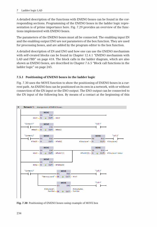
7 Ladder logic LAD
234
A detailed description of the functions with EN/ENO boxes can be found in the cor-responding sections. Programming of the EN/ENO boxes in the ladder logic repre-sentation is of prime importance here. Fig. 7.29 provides an overview of the func-tions implemented with EN/ENO boxes.
The parameters of the EN/ENO boxes must all be connected. The enabling input ENand the enabling output ENO are not parameters of the box function. They are usedfor processing boxes, and are added by the program editor to the box function.
A detailed description of EN and ENO and how one can use the EN/ENO mechanismwith self-created blocks can be found in Chapter 12.4.1 “EN/ENO mechanism withLAD and FBD” on page 418. The block calls in the ladder diagram, which are alsoshown as EN/ENO boxes, are described in Chapter 7.6.5 “Block call functions in theladder logic” on page 245.
7.5.1 Positioning of EN/ENO boxes in the ladder logic
Fig. 7.30 uses the MOVE function to show the positioning of EN/ENO boxes in a cur-rent path. An EN/ENO box can be positioned on its own in a network, with or withoutconnection of the EN input or the ENO output. The ENO output can be connected tothe EN input of the following box. By means of a contact at the beginning of this
Fig. 7.30 Positioning of EN/ENO boxes using example of MOVE box

7.5 Programming with EN/ENO boxes in the ladder logic
235
“main current path” it is possible to switch processing of the entire current path onand off. The signal state of the ENO output of the last box indicates by means of a“1” that the complete sequence has been processed without errors.
The ENO output of a box can be connected in parallel with the ENO output of a dif-ferent box if the boxes are present in separate current paths which commence onthe left-hand power rail. “Current” then flows in the subsequent path if one of thetwo boxes has completed the processing without errors.
If an EN/ENO box is positioned in a T branch, its ENO output can no longer be re-turned to the path at which the T branch commences.
7.5.2 Transfer functions in the ladder logic
Boxes with the following transfer functions are available in the programminglanguage LAD:
b Copy an operand or tag (MOVE)
b Read (FieldRead) and write (FieldWrite) a field component with variable index
b Copy a data area (MOVE_BLK) and copy a data area without interruption (UMOVE_BLK)
b Fill a data area (FILL_BLK) and fill a data area without interruption (UFILL_BLK)
b Exchange the bytes within a tag (SWAP)
A detailed description of the transfer functions is provided in Chapter 11.1 “Trans-fer functions” on page 356.
Fig. 7.31 shows an example of the programming of transfer functions. If the tag“Contact 1” changes the signal state from “0” to “1”, the MOVE and FILL_BLK boxeswill be executed.
The MOVE box copies the content of tag #Int1 to tag #Field1[1]. #Field1[1] is a com-ponent of the tag #Field1 with the same data type as the tag #Int1.
Fig. 7.31 Example of the transfer functions in the ladder logic
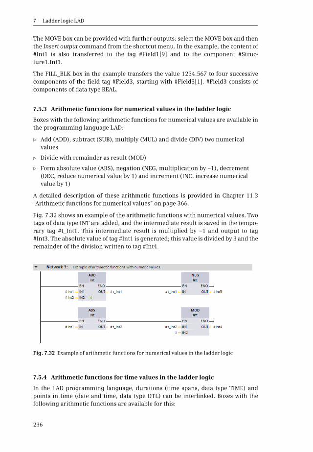
7 Ladder logic LAD
236
The MOVE box can be provided with further outputs: select the MOVE box and thenthe Insert output command from the shortcut menu. In the example, the content of#Int1 is also transferred to the tag #Field1[9] and to the component #Struc-ture1.Int1.
The FILL_BLK box in the example transfers the value 1234.567 to four successivecomponents of the field tag #Field3, starting with #Field3[1]. #Field3 consists ofcomponents of data type REAL.
7.5.3 Arithmetic functions for numerical values in the ladder logic
Boxes with the following arithmetic functions for numerical values are available inthe programming language LAD:
b Add (ADD), subtract (SUB), multiply (MUL) and divide (DIV) two numerical values
b Divide with remainder as result (MOD)
b Form absolute value (ABS), negation (NEG, multiplication by –1), decrement (DEC, reduce numerical value by 1) and increment (INC, increase numerical value by 1)
A detailed description of these arithmetic functions is provided in Chapter 11.3“Arithmetic functions for numerical values” on page 366.
Fig. 7.32 shows an example of the arithmetic functions with numerical values. Twotags of data type INT are added, and the intermediate result is saved in the tempo-rary tag #t_Int1. This intermediate result is multiplied by –1 and output to tag#Int3. The absolute value of tag #Int1 is generated; this value is divided by 3 and theremainder of the division written to tag #Int4.
7.5.4 Arithmetic functions for time values in the ladder logic
In the LAD programming language, durations (time spans, data type TIME) andpoints in time (date and time, data type DTL) can be interlinked. Boxes with thefollowing arithmetic functions are available for this:
Fig. 7.32 Example of arithmetic functions for numerical values in the ladder logic
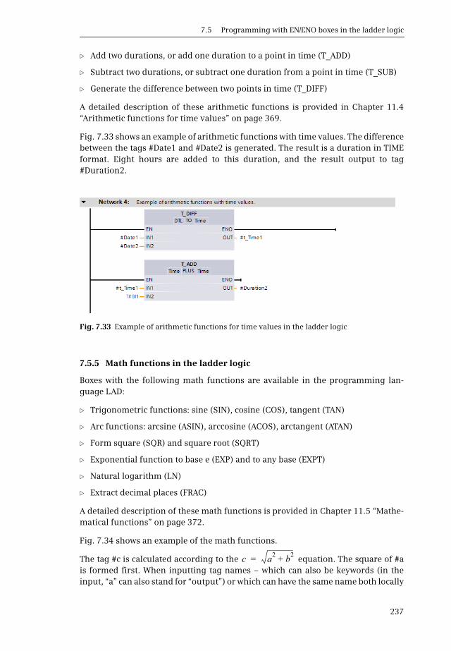
7.5 Programming with EN/ENO boxes in the ladder logic
237
b Add two durations, or add one duration to a point in time (T_ADD)
b Subtract two durations, or subtract one duration from a point in time (T_SUB)
b Generate the difference between two points in time (T_DIFF)
A detailed description of these arithmetic functions is provided in Chapter 11.4“Arithmetic functions for time values” on page 369.
Fig. 7.33 shows an example of arithmetic functions with time values. The differencebetween the tags #Date1 and #Date2 is generated. The result is a duration in TIMEformat. Eight hours are added to this duration, and the result output to tag#Duration2.
7.5.5 Math functions in the ladder logic
Boxes with the following math functions are available in the programming lan-guage LAD:
b Trigonometric functions: sine (SIN), cosine (COS), tangent (TAN)
b Arc functions: arcsine (ASIN), arccosine (ACOS), arctangent (ATAN)
b Form square (SQR) and square root (SQRT)
b Exponential function to base e (EXP) and to any base (EXPT)
b Natural logarithm (LN)
b Extract decimal places (FRAC)
A detailed description of these math functions is provided in Chapter 11.5 “Mathe-matical functions” on page 372.
Fig. 7.34 shows an example of the math functions.
The tag #c is calculated according to the equation. The square of #ais formed first. When inputting tag names – which can also be keywords (in theinput, “a” can also stand for “output”) or which can have the same name both locally
Fig. 7.33 Example of arithmetic functions for time values in the ladder logic
c a2 b2+=

7 Ladder logic LAD
238
and globally – the tag must be labeled accordingly: for a local tag with a precedingnumber sign (#), for a global tag with the name in quotation marks, and for an oper-and with a preceding percent sign (%).
In the example, the squares of #a and #b are stored temporarily and added. #t_Real1is used again for the buffer. The result of the square root extraction is saved in thetag #c.
7.5.6 Conversion functions in the ladder logic
Boxes with the following conversion functions are available in the programminglanguage LAD:
b CONV (conversion of BYTE, WORD, DWORD, SINT, INT, DINT, USINT,UINT, UDINT, REAL, LREAL, BCD16, BCD32)
b ROUND, FLOOR, CEIL, TRUNC (conversion of REAL, LREAL into SINT, INT,DINT, USINT, UINT, UDINT, REAL, LREAL)
b SCALE_X, NORM_X (scaling and standardization)
b T_CONV (conversion of TIME into DINT and vice versa)
b S_CONV, STRG_VAL, VAL_STRG (conversion of SINT, INT, DINT, USINT,UINT, UDINT, REAL into STRING and vice versa)
A detailed description of the conversion functions is provided in Chapter 11.6 “Con-version functions (Conversion of data type)” on page 376.
Fig. 7.35 shows an example of the conversion functions.
The conversion function CONV is used to convert a 7-digit BCD number into a DINTformat number and subsequently into REAL format (tag #t_Real2). The value of#t_Real2 is divided by 107 and converted into a fixed-point number between the lim-its of –150 and +250.
Fig. 7.34 Example of math functions in the ladder logic
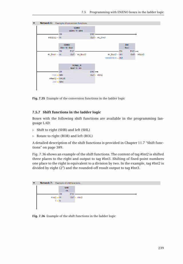
7.5 Programming with EN/ENO boxes in the ladder logic
239
7.5.7 Shift functions in the ladder logic
Boxes with the following shift functions are available in the programming lan-guage LAD:
b Shift to right (SHR) and left (SHL)
b Rotate to right (ROR) and left (ROL)
A detailed description of the shift functions is provided in Chapter 11.7 “Shift func-tions” on page 389.
Fig. 7.36 shows an example of the shift functions. The content of tag #Int2 is shiftedthree places to the right and output to tag #Int3. Shifting of fixed-point numbersone place to the right is equivalent to a division by two. In the example, tag #Int2 isdivided by eight (23) and the rounded-off result output to tag #Int3.
Fig. 7.35 Example of the conversion functions in the ladder logic
Fig. 7.36 Example of the shift functions in the ladder logic
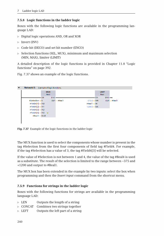
7 Ladder logic LAD
240
7.5.8 Logic functions in the ladder logic
Boxes with the following logic functions are available in the programming lan-guage LAD:
b Digital logic operations AND, OR and XOR
b Invert (INV)
b Code bit (DECO) and set bit number (ENCO)
b Selection functions (SEL, MUX), minimum and maximum selection (MIN, MAX), limiter (LIMIT)
A detailed description of the logic functions is provided in Chapter 11.8 “Logicfunctions” on page 392.
Fig. 7.37 shows an example of the logic functions.
The MUX function is used to select the components whose number is present in thetag #Selection from the first four components of field tag #Field4. For example,if the tag #Selection has a value of 3, the tag #Field4[3] will be selected.
If the value of #Selection is not between 1 and 4, the value of the tag #Real4 is usedas a substitute. The result of the selection is limited to the range between –375 and+1200 and output to #Real1.
The MUX box has been extended in the example by two inputs: select the box whenprogramming and then the Insert input command from the shortcut menu.
7.5.9 Functions for strings in the ladder logic
Boxes with the following functions for strings are available in the programminglanguage LAD:
b LEN Outputs the length of a stringb CONCAT Combines two strings togetherb LEFT Outputs the left part of a string
Fig. 7.37 Example of the logic functions in the ladder logic
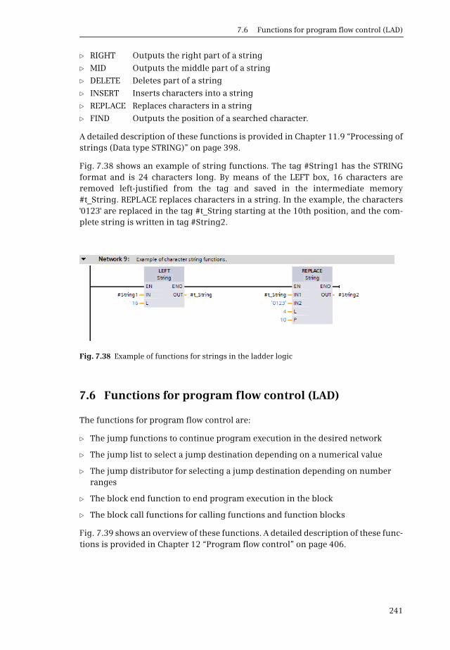
7.6 Functions for program flow control (LAD)
241
b RIGHT Outputs the right part of a string
b MID Outputs the middle part of a string
b DELETE Deletes part of a string
b INSERT Inserts characters into a string
b REPLACE Replaces characters in a string
b FIND Outputs the position of a searched character.
A detailed description of these functions is provided in Chapter 11.9 “Processing ofstrings (Data type STRING)” on page 398.
Fig. 7.38 shows an example of string functions. The tag #String1 has the STRINGformat and is 24 characters long. By means of the LEFT box, 16 characters areremoved left-justified from the tag and saved in the intermediate memory#t_String. REPLACE replaces characters in a string. In the example, the characters'0123' are replaced in the tag #t_String starting at the 10th position, and the com-plete string is written in tag #String2.
7.6 Functions for program flow control (LAD)
The functions for program flow control are:
b The jump functions to continue program execution in the desired network
b The jump list to select a jump destination depending on a numerical value
b The jump distributor for selecting a jump destination depending on number ranges
b The block end function to end program execution in the block
b The block call functions for calling functions and function blocks
Fig. 7.39 shows an overview of these functions. A detailed description of these func-tions is provided in Chapter 12 “Program flow control” on page 406.
Fig. 7.38 Example of functions for strings in the ladder logic
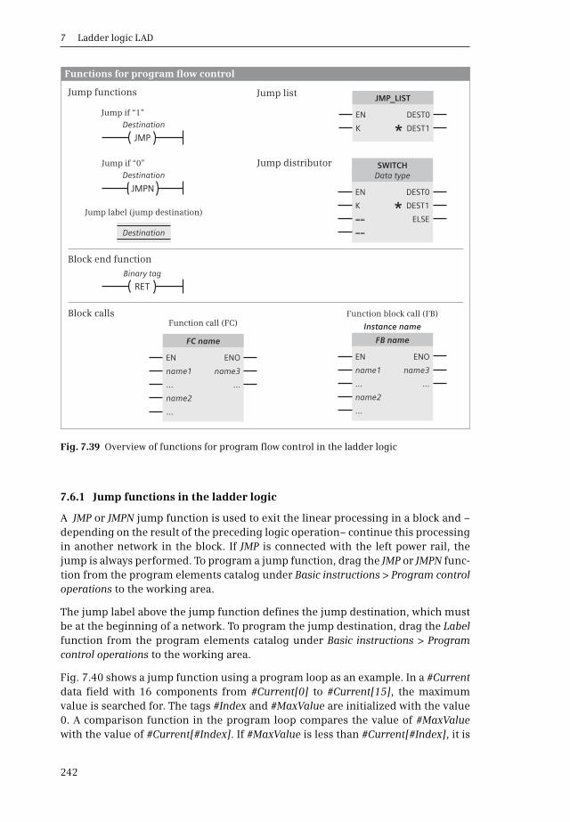
7 Ladder logic LAD
242
7.6.1 Jump functions in the ladder logic
A JMP or JMPN jump function is used to exit the linear processing in a block and –depending on the result of the preceding logic operation– continue this processingin another network in the block. If JMP is connected with the left power rail, thejump is always performed. To program a jump function, drag the JMP or JMPN func-tion from the program elements catalog under Basic instructions > Program controloperations to the working area.
The jump label above the jump function defines the jump destination, which mustbe at the beginning of a network. To program the jump destination, drag the Labelfunction from the program elements catalog under Basic instructions > Programcontrol operations to the working area.
Fig. 7.40 shows a jump function using a program loop as an example. In a #Currentdata field with 16 components from #Current[0] to #Current[15], the maximumvalue is searched for. The tags #Index and #MaxValue are initialized with the value0. A comparison function in the program loop compares the value of #MaxValuewith the value of #Current[#Index]. If #MaxValue is less than #Current[#Index], it is
Fig. 7.39 Overview of functions for program flow control in the ladder logic
Jump functions Jump list
Jump distributor
Block callsFunction call (FC)
Function block call (FB)
Block end function
Functions for program flow control
FC name
JMP_LIST
SWITCHData type
EN
EN
EN
name1
K
K
==
==
...
name2
...
name3
DEST1
DEST1
ELSE
...
ENO
DEST0
DEST0
Instance name
FB name
EN
name1
...
name2
...
name3
...
ENO
RETBinary tag
Jump if “1”
Jump if “0”
Jump label (jump destination)
JMP
JMPN
Destination
Destination
Destination
*
*
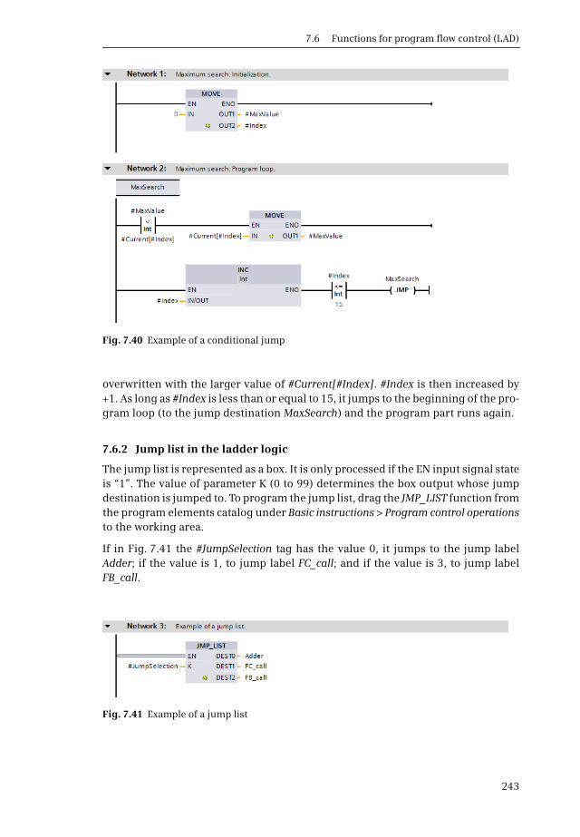
7.6 Functions for program flow control (LAD)
243
overwritten with the larger value of #Current[#Index]. #Index is then increased by+1. As long as #Index is less than or equal to 15, it jumps to the beginning of the pro-gram loop (to the jump destination MaxSearch) and the program part runs again.
7.6.2 Jump list in the ladder logic
The jump list is represented as a box. It is only processed if the EN input signal stateis “1”. The value of parameter K (0 to 99) determines the box output whose jumpdestination is jumped to. To program the jump list, drag the JMP_LIST function fromthe program elements catalog under Basic instructions > Program control operationsto the working area.
If in Fig. 7.41 the #JumpSelection tag has the value 0, it jumps to the jump labelAdder; if the value is 1, to jump label FC_call; and if the value is 3, to jump labelFB_call.
Fig. 7.40 Example of a conditional jump
Fig. 7.41 Example of a jump list
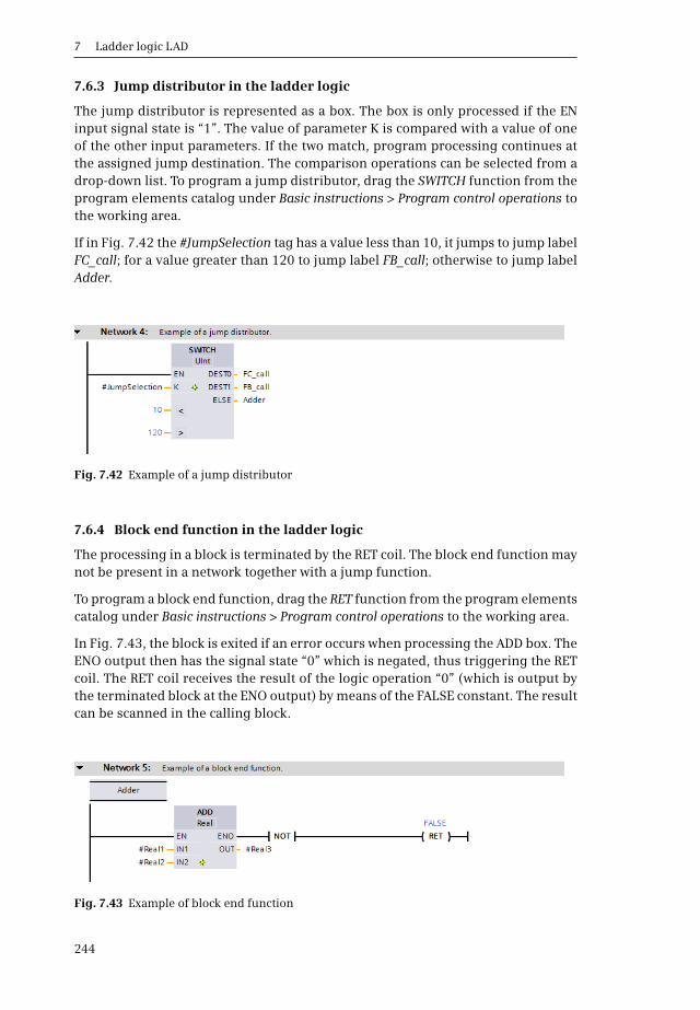
7 Ladder logic LAD
244
7.6.3 Jump distributor in the ladder logic
The jump distributor is represented as a box. The box is only processed if the ENinput signal state is “1”. The value of parameter K is compared with a value of oneof the other input parameters. If the two match, program processing continues atthe assigned jump destination. The comparison operations can be selected from adrop-down list. To program a jump distributor, drag the SWITCH function from theprogram elements catalog under Basic instructions > Program control operations tothe working area.
If in Fig. 7.42 the #JumpSelection tag has a value less than 10, it jumps to jump labelFC_call; for a value greater than 120 to jump label FB_call; otherwise to jump labelAdder.
7.6.4 Block end function in the ladder logic
The processing in a block is terminated by the RET coil. The block end function maynot be present in a network together with a jump function.
To program a block end function, drag the RET function from the program elementscatalog under Basic instructions > Program control operations to the working area.
In Fig. 7.43, the block is exited if an error occurs when processing the ADD box. TheENO output then has the signal state “0” which is negated, thus triggering the RETcoil. The RET coil receives the result of the logic operation “0” (which is output bythe terminated block at the ENO output) by means of the FALSE constant. The resultcan be scanned in the calling block.
Fig. 7.42 Example of a jump distributor
Fig. 7.43 Example of block end function

7.6 Functions for program flow control (LAD)
245
7.6.5 Block call functions in the ladder logic
Calling of blocks is represented by EN/ENO boxes. With functions (FC), the blockname is present quasi as a function name in the box; with function blocks, theinstance name (the name of the instance data block or of the local instance) is addi-tionally present above the box.
A block call is programmed by opening the Program blocks folder in the project treeand dragging the desired block to the working area.
In the example in Fig. 7.44, if the signal state is “1” on the “Input 2” tag, the function“Adder_2” is called. In the event of an error in the function “Adder_2” (the ENO out-put then has signal state “0”), the tag #AddError is also set to signal state “0”. Theprogram processing is then ended in the block and #AddError is specified as returntag. This means that if the processing in the block “Adder_2” is faulty, the ENO out-put of the ended block is set to signal state “0”.
In the example in Fig. 7.45 , the “Totalizer” function block is called. Its instance datais present in the data block “Totalizer_DB”.
Fig. 7.44 Example of calling a function (FC)
Fig. 7.45 Example of calling a function block

8 Function block diagram FBD
246
8 Function block diagram FBD
8.1 Introduction
This chapter describes programming with function block diagram (FBD); it usesexamples to show how the program functions are represented in FBD. You can finda description of the individual functions, e.g. comparison functions, in Chapter 10“Basic functions” on page 328.
Use of the program and symbol editor, which generally applies to all programminglanguages is described in Chapter 6 “Program editor” on page 178.
FBD is used to program the contents of blocks (the user program). What blocks are,and how they are created, is described in Chapters 5.3 “Programming blocks” onpage 125 and 6.3 “Programming a code block” on page 183.
8.1.1 Programming with function block diagram in general
You use FBD to program the control function of the programmable controller – theuser program or control program. The user program is organized in different typesof blocks. A block is divided into sections referred to as “networks”. Each networkcontains at least one logic operation, which can also have an extremely complexstructure. Each network is terminated by at least one box.
Fig. 8.1 shows the structure of a block with the FBD program. Located at the begin-ning of the program is the block title, comprising the block heading and block com-ment. Heading and comment are optional. These are followed by the first networkwith its number, heading, and comment. Heading and comment are also optionalfor the networks. The first network shows a logic operation as example with ANDand OR boxes, a memory function within the logic operation, and two assignmentsas termination of the logic operation. The second network shows the processing ofEN/ENO boxes. Three of these are arranged in series, one box is on its own in thenetwork. A block is not terminated by a special network or function, you simply fin-ish the program input.
The program editor constructs an FBD network from left to right: position the firstprogram element underneath the network comment, and insert further programelements at its output. The boxes with binary logic operations can be provided withfurther inputs. Box outputs cannot be directly connected to each other.
A logic operation must always be terminated, for example by an assignment.The assignment controls a binary tag using the result of the logic operation.
“Open” parallel branches can lead out from the top logic operation and not be“wired back” to the top logic operation; these are known as “T branches”. In these
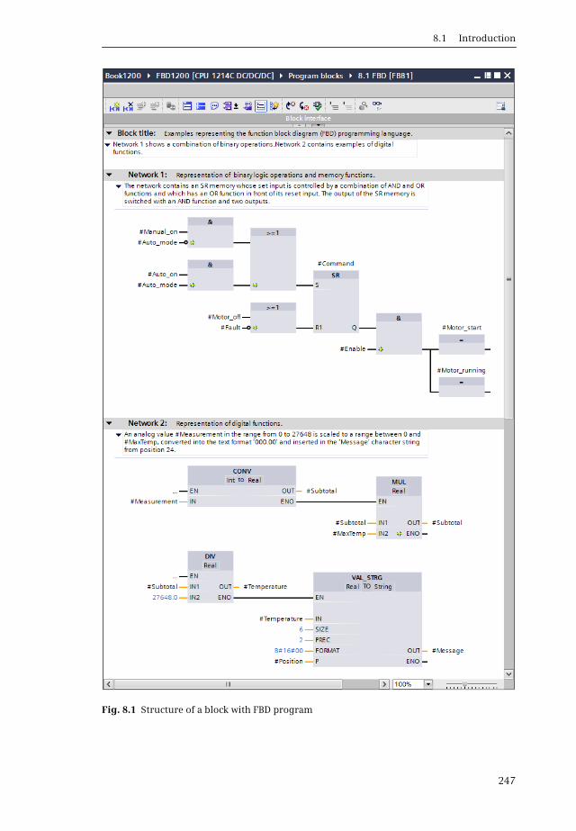
8.1 Introduction
247
Fig. 8.1 Structure of a block with FBD program
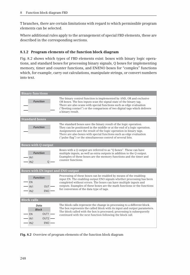
8 Function block diagram FBD
248
T branches, there are certain limitations with regard to which permissible programelements can be selected.
Where additional rules apply to the arrangement of special FBD elements, these aredescribed in the corresponding sections.
8.1.2 Program elements of the function block diagram
Fig. 8.2 shows which types of FBD elements exist: boxes with binary logic opera-tions, and standard boxes for processing binary signals, Q boxes for implementingmemory, timer and counter functions, and EN/ENO boxes for “complex” functionswhich, for example, carry out calculations, manipulate strings, or convert numbersinto text.
Fig. 8.2 Overview of program elements of the function block diagram
The binary control function is implemented by AND, OR and exclusive OR boxes. The box inputs scan the signal state of the binary tag. There are also scans with special functions such as edge evaluation (“fleeting contact”) or the comparison of two digital tags which delivers a binary result.
The standard boxes save the binary result of the logic operation. They can be positioned in the middle or at the end of a logic operation. Assignments save the result of the logic operation in binary tags. There are also boxes with special functions such as edge evaluation (“pulse flag”) or the simultaneous control of several bits.
Boxes with a Q output are referred to as “Q boxes”. These can have multiple inputs, as well as extra outputs in addition to the Q output. Examples of these boxes are the memory functions and the timer and counter functions.
Processing of these boxes can be enabled by means of the enabling input EN. The enabling output ENO signals whether processing has been completed without errors. The boxes can have multiple inputs and outputs. Examples of these boxes are the math functions or the functions for conversion of the data type of tags.
The block calls represent the change in processing to a different block. The box represents the called block with its input and output parameters. The block called with the box is processed; processing is subsequently continued with the next function following the block call.
Function
Function
Function
Function
Block
Q
OUT
OUT1
ENO
OUT2
ENO
IN1
EN
EN
IN2
IN2
IN2
IN1
IN1
Data
Binary functions
Standard boxes
Boxes with Q output
Boxes with EN input and ENO output
Block calls

8.2 Programming of binary logic operations (FBD)
249
Most program elements must be provided with tags or operand addresses at thebox inputs and outputs. It is best if you initially position all program elements in alogic operation and subsequently label them.
8.2 Programming of binary logic operations (FBD)
The binary logic operations are carried out in the function block diagram using theAND, OR, and exclusive OR boxes. The binary tags for the logic operation can bescanned for signal state “1” or “0”. The binary results of other boxes can also beincluded, e.g. the evaluation of a signal edge, the validity checking of floating-pointnumbers, or the comparison of two digital tags (Fig. 8.3).
Fig. 8.3 Overview of binary logic operations in the function block diagram
Binary tags
Binary tag Binary tag
Binary tags
AND function OR function Exclusive OR function
Scan for “loating-point value OK” Scan for “Floating-point value not OK”
Comparison function
Floating-point tag Floating-point tag
Positive edge of a binary tag Negative edge of a binary tag
Scan for signal state “1” Scan for signal state “0”
Edge trigger flag Edge trigger flag
Digital tag 1 Digital tag 2
Binary logic operations
& >=1 X
Data typeFunction
Function Function
P
OK
N
NOT_OK

8 Function block diagram FBD
250
8.2.1 Scanning for signal states “1” and “0”
The binary functions scan the binary tags at the function inputs before they link thesignal states together. The scan can be made for signal state “1” or “0”. When scan-ning for signal state “1”, the function input leads directly to the box. You can recog-nize the scanning for signal state “0” by means of the negation circle at the input ofthe function.
Scanning for signal state “1” delivers a result “1” if the scanned binary tag has thestatus “1”, and a result “0” if the status is “0”. Scanning for signal state “0” negatesthe result, i.e. the result of the scan is now “1” if the status of the scanned binary tagis “0”. The binary functions link the result of the scan, in other words the resultwhich is present “directly” on the box. Using these two possibilities for scanning bi-nary tags, you can handle connected NO and NC contacts in the same functionalmanner.
Example: Fig. 8.4 shows a sensor connected to the programmable controller whichis scanned for signal state “1” (left-hand side) and for signal state “0” (right-handside). The result of the scan is connected directly to a contactor.
When scanning for signal state “1” (left-hand side), the result of the scan is equal tothe signal state of the sensor: if sensor S1 is open, input %I1.0 has the signal state“0” and the logic operation is not fulfilled. Contactor K1 controlled by output %Q4.0
Fig. 8.4 Scanning for signal states “1” and “0”
S1 S2
C1 C2C1 C2
S1 S2
%I1.0 %I1.1
%Q4.0 %Q4.1%Q4.0 %Q4.1
%I1.0 %I1.1
“0”
“1”“1”
“1”“1”
“0”“0”
“0”
Scan for signal state “1” Scan for signal state “0”
Sensor activated
Sensor activated
& & & &
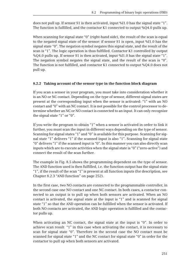
8.2 Programming of binary logic operations (FBD)
251
does not pull up. If sensor S1 is then activated, input %I1.0 has the signal state “1”.The function is fulfilled, and the contactor K1 connected to output %Q4.0 pulls up.
When scanning for signal state “0” (right-hand side), the result of the scan is equalto the negated signal state of the sensor: if sensor S1 is open, input %I1.0 has thesignal state “0”. The negation symbol negates this signal state, and the result of thescan is “1”. The logic operation is thus fulfilled. Contactor K1 controlled by output%Q4.0 pulls up. If sensor S1 is then activated, input %I1.0 has the signal state “1”.The negation symbol negates the signal state, and the result of the scan is “0”.The function is not fulfilled, and contactor K1 connected to output %Q4.0 does notpull up.
8.2.2 Taking account of the sensor type in the function block diagram
If you scan a sensor in your program, you must take into consideration whether itis an NO or NC contact. Depending on the type of sensor, different signal states arepresent at the corresponding input when the sensor is activated: “1” with an NOcontact and “0” with an NC contact. It is not possible for the control processor to de-termine whether an NC or NO contact is connected to an input. It can only recognizethe signal state “1” or “0”.
If you write the program to obtain “1” when a sensor is activated in order to link itfurther, you must scan the input in different ways depending on the type of sensor.Scanning for signal states “1” and “0” is available for this purpose. Scanning for sig-nal state “1” delivers “1” if the scanned input is also “1”. Scanning for signal state“0” delivers “1” if the scanned input is “0”. In this manner you can also directly scaninputs which are to execute activities when the signal state is “0” (“zero-active”) andconnect the result of the scan further.
The example in Fig. 8.5 shows the programming dependent on the type of sensor.The AND function used is then fulfilled, i.e. the function output has the signal state“1”, if the result of the scan “1” is present at all function inputs (for description, seeChapter 8.2.3 “AND function” on page 252).
In the first case, two NO contacts are connected to the programmable controller, inthe second case one NO contact and one NC contact. In both cases, a contactor con-nected to an output is to pull up when both sensors are activated. When an NOcontact is activated, the signal state at the input is “1” and is scanned for signalstate “1” so that the AND operation can be fulfilled when the sensor is activated. Ifboth NO contacts are activated, the AND logic operation is fulfilled and the contac-tor pulls up.
When activating an NC contact, the signal state at the input is “0”. In order toachieve scan result “1” in this case when activating the contact, it is necessary toscan for signal state “0”. Therefore in the second case the NO contact must bescanned for signal state “1” and the NC contact for signal state “0” in order for thecontactor to pull up when both sensors are activated.
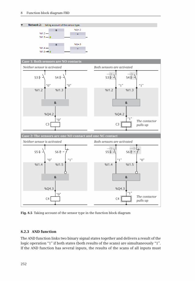
8 Function block diagram FBD
252
8.2.3 AND function
The AND function links two binary signal states together and delivers a result of thelogic operation “1” if both states (both results of the scans) are simultaneously “1”.If the AND function has several inputs, the results of the scans of all inputs must
Fig. 8.5 Taking account of the sensor type in the function block diagram
Neither sensor is activated
Neither sensor is activated
Both sensors are activated
Both sensors are activated
The contactor pulls up
The contactor pulls up
S3
S5
S3
S5
S4
S6
S4
S6
C3
C4
C3
C4
%I1.2
%I1.4
%I1.2
%I1.4
%I1.3
%I1.5
%I1.3
%I1.5
%Q4.2
%Q4.3
%Q4.2
%Q4.3
“0”
“0” “0”
“0” “1”
“1”
“1”
“1”
“1”
“1”
“0”
“0”
Case 1: Both sensors are NO contacts
Case 2: The sensors are one NO contact and one NC contact
&
&
&
&
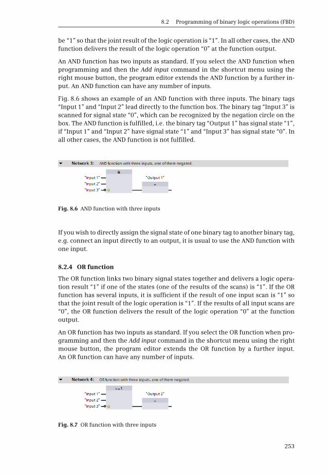
8.2 Programming of binary logic operations (FBD)
253
be “1” so that the joint result of the logic operation is “1”. In all other cases, the ANDfunction delivers the result of the logic operation “0” at the function output.
An AND function has two inputs as standard. If you select the AND function whenprogramming and then the Add input command in the shortcut menu using theright mouse button, the program editor extends the AND function by a further in-put. An AND function can have any number of inputs.
Fig. 8.6 shows an example of an AND function with three inputs. The binary tags“Input 1” and “Input 2” lead directly to the function box. The binary tag “Input 3” isscanned for signal state “0”, which can be recognized by the negation circle on thebox. The AND function is fulfilled, i.e. the binary tag “Output 1” has signal state “1”,if “Input 1” and “Input 2” have signal state “1” and “Input 3” has signal state “0”. Inall other cases, the AND function is not fulfilled.
If you wish to directly assign the signal state of one binary tag to another binary tag,e.g. connect an input directly to an output, it is usual to use the AND function withone input.
8.2.4 OR function
The OR function links two binary signal states together and delivers a logic opera-tion result “1” if one of the states (one of the results of the scans) is “1”. If the ORfunction has several inputs, it is sufficient if the result of one input scan is “1” sothat the joint result of the logic operation is “1”. If the results of all input scans are“0”, the OR function delivers the result of the logic operation “0” at the functionoutput.
An OR function has two inputs as standard. If you select the OR function when pro-gramming and then the Add input command in the shortcut menu using the rightmouse button, the program editor extends the OR function by a further input.An OR function can have any number of inputs.
Fig. 8.6 AND function with three inputs
Fig. 8.7 OR function with three inputs

8 Function block diagram FBD
254
Fig. 8.7 shows an example of an OR function with three inputs. The binary tags“Input 1” and “Input 2” lead directly to the function box. The binary tag “Input 3” isscanned for signal state “0”, which can be recognized by the negation circle on thebox. The OR function is not fulfilled, i.e. the binary tag “Output 2” has signal state“0”, if “Input 1” and “Input 2” have signal state “0” and “Input 3” has signal state “1”.In all other cases, the OR function is fulfilled.
8.2.5 Exclusive OR function
The exclusive OR function (non-equivalence function) links two binary signal statestogether and delivers a logic operation result “1” if the two states (both results ofthe scans) differ. It delivers a result of the logic operation “0” if the two states (bothresults of the scans) are the same.
You can also program an exclusive OR function with more than two inputs; the ex-clusive OR function is then fulfilled if an odd number of function inputs deliversscan result “1”.
An exclusive OR function has two inputs as standard. If you select the exclusiveOR function when programming and then the Add input command in the shortcutmenu using the right mouse button, the program editor extends the exclusiveOR function by a further input. An exclusive OR function can have any number ofinputs.
Fig. 8.8 shows an example of an exclusive OR function with two inputs. The binarytags “Input 1” and “Input 2” lead directly to the function box. The exclusive OR func-tion is fulfilled, i.e. the binary tag “Output 3” has signal state “1”, if “Input 1” and“Input 2” have different signal states. If the signal states of “Input 1” and “Input 2”are the same, the exclusive OR function is not fulfilled.
8.2.6 Mixed binary logic operations
You can combine binary functions with each other, e.g. several AND functions leadto an OR function or two OR functions lead to an exclusive OR function. Examplesare shown in Fig. 8.9.
With which signal combination in Fig. 8.9 is the binary tag “Output 4” set to signalstate “1”? Firstly, “Input 5” and “Input 6” must have different signal states if theAND function at the end of the logic operation is to be fulfilled. The other conditionis that either “Input 1” and “Input 2” both have signal state “1” or that “Input 3” and“Input 4” have different signal states.
Fig. 8.8 Exclusive OR function with two inputs
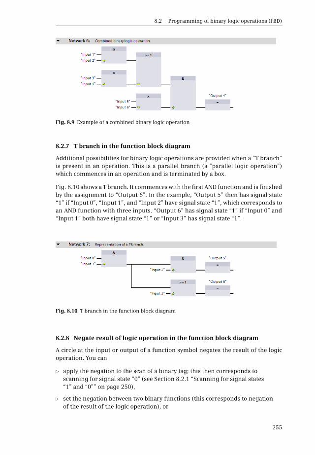
8.2 Programming of binary logic operations (FBD)
255
8.2.7 T branch in the function block diagram
Additional possibilities for binary logic operations are provided when a “T branch”is present in an operation. This is a parallel branch (a “parallel logic operation”)which commences in an operation and is terminated by a box.
Fig. 8.10 shows a T branch. It commences with the first AND function and is finishedby the assignment to “Output 6”. In the example, “Output 5” then has signal state“1” if “Input 0”, “Input 1”, and “Input 2” have signal state “1”, which corresponds toan AND function with three inputs. “Output 6” has signal state “1” if “Input 0” and“Input 1” both have signal state “1” or “Input 3” has signal state “1”.
8.2.8 Negate result of logic operation in the function block diagram
A circle at the input or output of a function symbol negates the result of the logicoperation. You can
b apply the negation to the scan of a binary tag; this then corresponds to scanning for signal state “0” (see Section 8.2.1 “Scanning for signal states “1” and “0”” on page 250),
b set the negation between two binary functions (this corresponds to negation of the result of the logic operation), or
Fig. 8.9 Example of a combined binary logic operation
Fig. 8.10 T branch in the function block diagram

8 Function block diagram FBD
256
b position the negation at the output of a binary function (e.g. if you wish to set a binary tag and the logic operation is not fulfilled, i.e. the result of the logic operation = “0”).
Program the negation using the Invert RLO program element from the favorites ofthe program editor or from the program elements catalog under General. You candrag the Invert RLO element to an input or output of a box using the mouse, or selectthe input or output and click on Invert RLO. If you wish to cancel a negation, dragInvert RLO over again, or select the negation and click on Invert RLO.
Fig. 8.11 shows three examples of the negation of a function output. A NAND func-tion is an AND function with negated output: the output only has signal state “0” ifthe scan result “1” is present at all inputs. A NOR function is an OR function withnegated output: the output only has signal state “1” if neither of the inputs has thescan result “1”. An exclusive OR function with a negated output is also referred toas an inclusive OR function (equivalence function): The output only has signal state“1” if the scan results are the same for both inputs. If more than two inputs are pres-ent, an even number of inputs must have the scan result “1” so that the inclusive ORfunction is fulfilled.
8.2.9 Edge evaluation of binary tags in the function block diagram
The edge evaluation of a binary tag has the signal state “1” for one processing cycleif the signal state of the binary tag named above it changes from “0” to “1” (P box,rising edge) or from “1” to “0” (N box, falling edge). It responds like a “fleetingcontact”. This “pulse” can be linked further.
The edge trigger flag is named underneath the edge box. This is a flag or data bitwhich saves the signal state of the binary tag. The signal edge is recognized by com-paring the signal states of binary tags and edge trigger flags (see also Chapter 10.3“Edge evaluation” on page 338).
Fig. 8.11 Negating the result of the logic operation, example of a negated function output
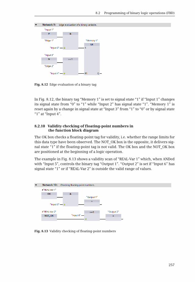
8.2 Programming of binary logic operations (FBD)
257
In Fig. 8.12, the binary tag “Memory 1” is set to signal state “1” if “Input 1” changesits signal state from “0” to “1” while “Input 2” has signal state “1”. “Memory 1” isreset again by a change in signal state at “Input 3” from “1” to “0” or by signal state“1” at “Input 4”.
8.2.10 Validity checking of floating-point numbers in the function block diagram
The OK box checks a floating-point tag for validity, i.e. whether the range limits forthis data type have been observed. The NOT_OK box is the opposite, it delivers sig-nal state “1” if the floating-point tag is not valid. The OK box and the NOT_OK boxare positioned at the beginning of a logic operation.
The example in Fig. 8.13 shows a validity scan of “REAL-Var 1” which, when ANDedwith “Input 5”, controls the binary tag “Output 1”. “Output 2” is set if “Input 6” hassignal state “1” or if “REAL-Var 2” is outside the valid range of values.
Fig. 8.12 Edge evaluation of a binary tag
Fig. 8.13 Validity checking of floating-point numbers
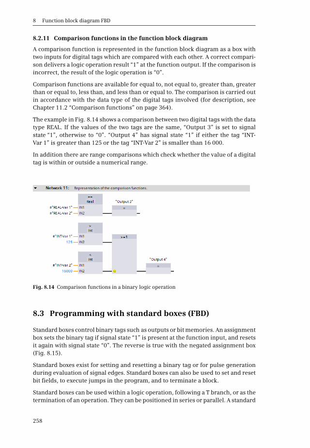
8 Function block diagram FBD
258
8.2.11 Comparison functions in the function block diagram
A comparison function is represented in the function block diagram as a box withtwo inputs for digital tags which are compared with each other. A correct compari-son delivers a logic operation result “1” at the function output. If the comparison isincorrect, the result of the logic operation is “0”.
Comparison functions are available for equal to, not equal to, greater than, greaterthan or equal to, less than, and less than or equal to. The comparison is carried outin accordance with the data type of the digital tags involved (for description, seeChapter 11.2 “Comparison functions” on page 364).
The example in Fig. 8.14 shows a comparison between two digital tags with the datatype REAL. If the values of the two tags are the same, “Output 3” is set to signalstate “1”, otherwise to “0”. “Output 4” has signal state “1” if either the tag “INT-Var 1” is greater than 125 or the tag “INT-Var 2” is smaller than 16 000.
In addition there are range comparisons which check whether the value of a digitaltag is within or outside a numerical range.
8.3 Programming with standard boxes (FBD)
Standard boxes control binary tags such as outputs or bit memories. An assignmentbox sets the binary tag if signal state “1” is present at the function input, and resetsit again with signal state “0”. The reverse is true with the negated assignment box(Fig. 8.15).
Standard boxes exist for setting and resetting a binary tag or for pulse generationduring evaluation of signal edges. Standard boxes can also be used to set and resetbit fields, to execute jumps in the program, and to terminate a block.
Standard boxes can be used within a logic operation, following a T branch, or as thetermination of an operation. They can be positioned in series or parallel. A standard
Fig. 8.14 Comparison functions in a binary logic operation
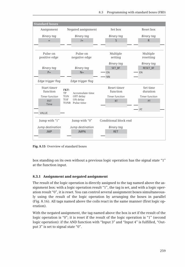
8.3 Programming with standard boxes (FBD)
259
box standing on its own without a previous logic operation has the signal state “1”at the function input.
8.3.1 Assignment and negated assignment
The result of the logic operation is directly assigned to the tag named above the as-signment box: with a logic operation result “1”, the tag is set, and with a logic oper-ation result “0”, it is reset. You can control several assignment boxes simultaneous-ly using the result of the logic operation by arranging the boxes in parallel(Fig. 8.16). All tags named above the coils react in the same manner (first logic op-eration).
With the negated assignment, the tag named above the box is set if the result of thelogic operation is “0”; it is reset if the result of the logic operation is “1” (secondlogic operation): if the AND function with “Input 3” and “Input 4” is fulfilled, “Out-put 3” is set to signal state “0”.
Fig. 8.15 Overview of standard boxes
Start timerfunction
Reset timerfunction
Set timeduration
Timer function Timer function Timer function
Standard boxes
FKTTime
RT PT
VALUEPT
FKT:TP Accumulate timeTON OFF delayTOF ON delayTONR Pulse time
Negated assignment Reset box
Binary tag Binary tagBinary tag Binary tag
Assignment Set box
= S/= R
Pulse onpositive edge
Pulse onnegative edge
Binary tag Binary tag
Edge trigger flag Edge trigger flag
P= N=
Multiplesetting
Multipleresetting
Binary tag Binary tagSET_BF RESET_BF
EN EN
NN
Jump with “1” Jump with “0”
Jump destination Jump destinationJMP JMPN
Conditional block end
Binary tagRET
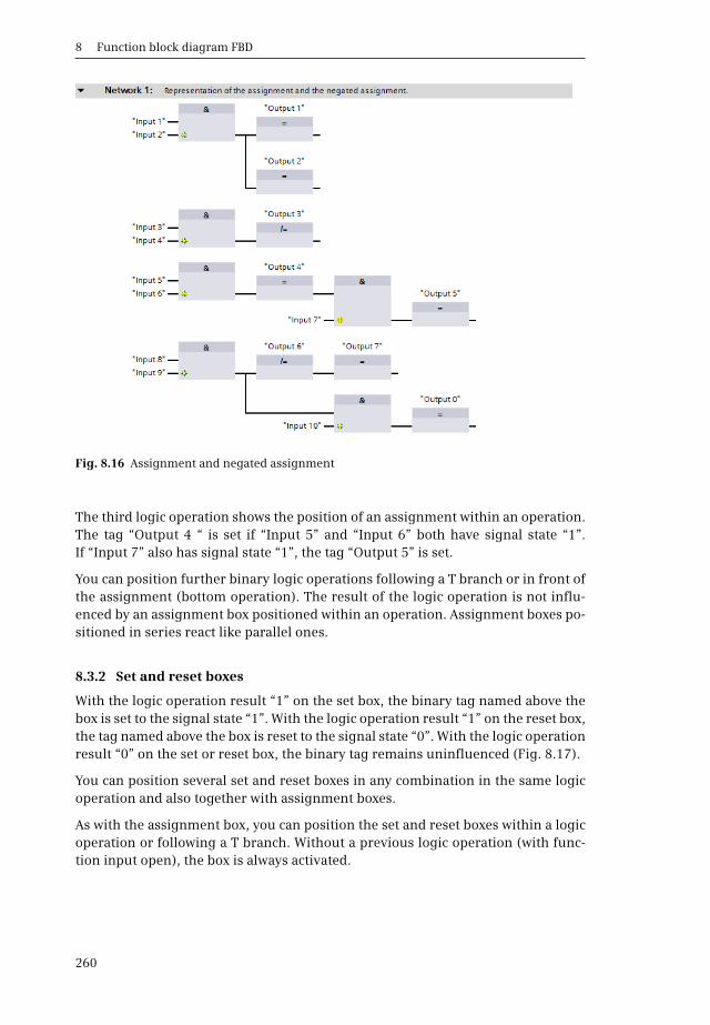
8 Function block diagram FBD
260
The third logic operation shows the position of an assignment within an operation.The tag “Output 4 “ is set if “Input 5” and “Input 6” both have signal state “1”.If “Input 7” also has signal state “1”, the tag “Output 5” is set.
You can position further binary logic operations following a T branch or in front ofthe assignment (bottom operation). The result of the logic operation is not influ-enced by an assignment box positioned within an operation. Assignment boxes po-sitioned in series react like parallel ones.
8.3.2 Set and reset boxes
With the logic operation result “1” on the set box, the binary tag named above thebox is set to the signal state “1”. With the logic operation result “1” on the reset box,the tag named above the box is reset to the signal state “0”. With the logic operationresult “0” on the set or reset box, the binary tag remains uninfluenced (Fig. 8.17).
You can position several set and reset boxes in any combination in the same logicoperation and also together with assignment boxes.
As with the assignment box, you can position the set and reset boxes within a logicoperation or following a T branch. Without a previous logic operation (with func-tion input open), the box is always activated.
Fig. 8.16 Assignment and negated assignment

8.3 Programming with standard boxes (FBD)
261
8.3.3 Edge evaluation with pulse output in the function block diagram
The P= and N= boxes are available for edge evaluation with pulse output. The binarytag named above the P= box is set for the duration of one program cycle if the logicoperation result of the previous operation changes from signal state “0” to “1” (ris-ing edge).
With the N= box, the binary tag named above the box is set for the duration of oneprogram cycle with a falling edge of the previous operation (change in logic opera-tion result from “1” to “0”) (Fig. 8.18).
The binary tag named above the box is referred to as a “Pulse bit memory”. Suitablefor pulse bit memories are operand types which are not connected “outside” tomodules, for example tags from the bit memory or data areas. The edge trigger flagis named under the box, and must be a different tag for each edge evaluation (seeChapter 10.3 “Edge evaluation” on page 338).
The edge boxes can be positioned within a logic operation or terminate an opera-tion. Edge boxes can also be programmed following a T branch.
Fig. 8.17 Set and reset boxes
Fig. 8.18 Edge evaluation of logic operation result (with “pulse bit memory”)

8 Function block diagram FBD
262
8.3.4 Multiple setting and resetting (filling of bit field) in the function block diagram
With the logic operation result “1” at the EN input, the SET_BF box sets a bit field tosignal state “1”. The bit field is defined by the start tag named above the box and thenumber of bits at the function input N. With the logic operation result “1”, theRESET_BF box resets the bits in the bit field.
There is no response if the result of the logic operation at the EN input is “0”. If theSET_BF and RESET_BF boxes do not have a previous operation, they are always exe-cuted.
In the example in Fig. 8.19, the bit field for the SET_BF box is defined by the starttag “Bitfield0” which is followed by seven bits (thus a total of eight bits). The bit fieldfor the RESET_BF box is in the data block “Data80”, commences with the field(binary) component Bitfield[1], and ends after 15 subsequent bits.
8.3.5 Starting IEC timer functions in the function block diagram with standard boxes
You can use the timer functions to implement timing processes in theprogram such as waiting and monitoring times, measurement of a time interval, orthe generation of pulses. An IEC timer function can be started with two differentprogram elements: with a standard box or with a Q box (see Chapter 8.4.5 “Control-ling IEC timer functions in the function block diagram with Q boxes” on page 267).Both variants are equally useful. A detailed description of the timer functions isprovided in Chapter 10.4 “Time functions” on page 344.
A timer function can be started with one of the four behavior patterns TP, TON, TOF,and TONR. A timer function requires internal data for each application. You canspecify where this data is to be saved when programming: For the Single instanceentry in its own data block with the data type IEC_TIMER and for the Multi-instance
Fig. 8.19 Filling of bit field with SET_BF and RESET_BF
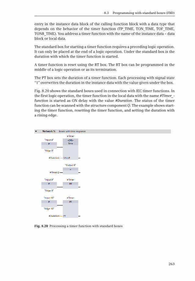
8.3 Programming with standard boxes (FBD)
263
entry in the instance data block of the calling function block with a data type thatdepends on the behavior of the timer function (TP_TIME, TON_TIME, TOF_TIME,TONR_TIME). You address a timer function with the name of the instance data – datablock or local data.
The standard box for starting a timer function requires a preceding logic operation.It can only be placed at the end of a logic operation. Under the standard box is theduration with which the timer function is started.
A timer function is reset using the RT box. The RT box can be programmed in themiddle of a logic operation or as its termination.
The PT box sets the duration of a timer function. Each processing with signal state“1” overwrites the duration in the instance data with the value given under the box.
Fig. 8.20 shows the standard boxes used in connection with IEC timer functions. Inthe first logic operation, the timer function in the local data with the name #Timer_-function is started as ON delay with the value #Duration. The status of the timerfunction can be scanned with the structure component Q. The example shows start-ing the timer function, resetting the timer function, and setting the duration witha rising edge.
Fig. 8.20 Processing a timer function with standard boxes
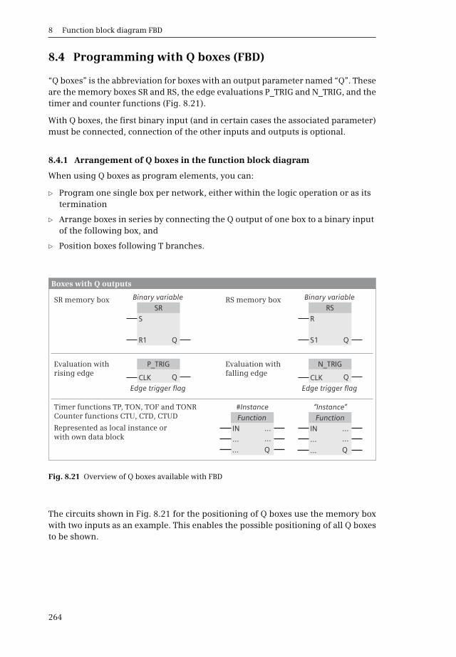
8 Function block diagram FBD
264
8.4 Programming with Q boxes (FBD)
“Q boxes” is the abbreviation for boxes with an output parameter named “Q”. Theseare the memory boxes SR and RS, the edge evaluations P_TRIG and N_TRIG, and thetimer and counter functions (Fig. 8.21).
With Q boxes, the first binary input (and in certain cases the associated parameter)must be connected, connection of the other inputs and outputs is optional.
8.4.1 Arrangement of Q boxes in the function block diagram
When using Q boxes as program elements, you can:
b Program one single box per network, either within the logic operation or as its termination
b Arrange boxes in series by connecting the Q output of one box to a binary input of the following box, and
b Position boxes following T branches.
The circuits shown in Fig. 8.21 for the positioning of Q boxes use the memory boxwith two inputs as an example. This enables the possible positioning of all Q boxesto be shown.
Fig. 8.21 Overview of Q boxes available with FBD
RS memory boxSR memory box
Evaluation with falling edge
Evaluation with rising edge
Timer functions TP, TON, TOF and TONRCounter functions CTU, CTD, CTUD
Represented as local instance or with own data block
Binary variable Binary variable
SR RS
S R
R1 S1
Edge trigger flag Edge trigger flag
P_TRIG N_TRIG
CLK CLKQ
Q Q
Q
FunctionFunction#Instance
ININ
...
...
...
...
......
...
Q
...
Q
“Instance”
Boxes with Q outputs
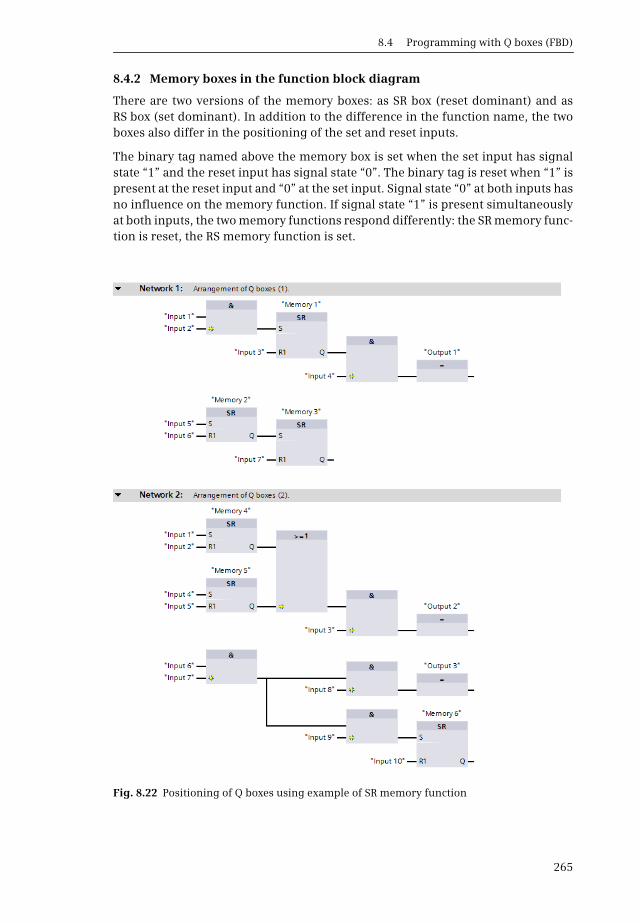
8.4 Programming with Q boxes (FBD)
265
8.4.2 Memory boxes in the function block diagram
There are two versions of the memory boxes: as SR box (reset dominant) and asRS box (set dominant). In addition to the difference in the function name, the twoboxes also differ in the positioning of the set and reset inputs.
The binary tag named above the memory box is set when the set input has signalstate “1” and the reset input has signal state “0”. The binary tag is reset when “1” ispresent at the reset input and “0” at the set input. Signal state “0” at both inputs hasno influence on the memory function. If signal state “1” is present simultaneouslyat both inputs, the two memory functions respond differently: the SR memory func-tion is reset, the RS memory function is set.
Fig. 8.22 Positioning of Q boxes using example of SR memory function
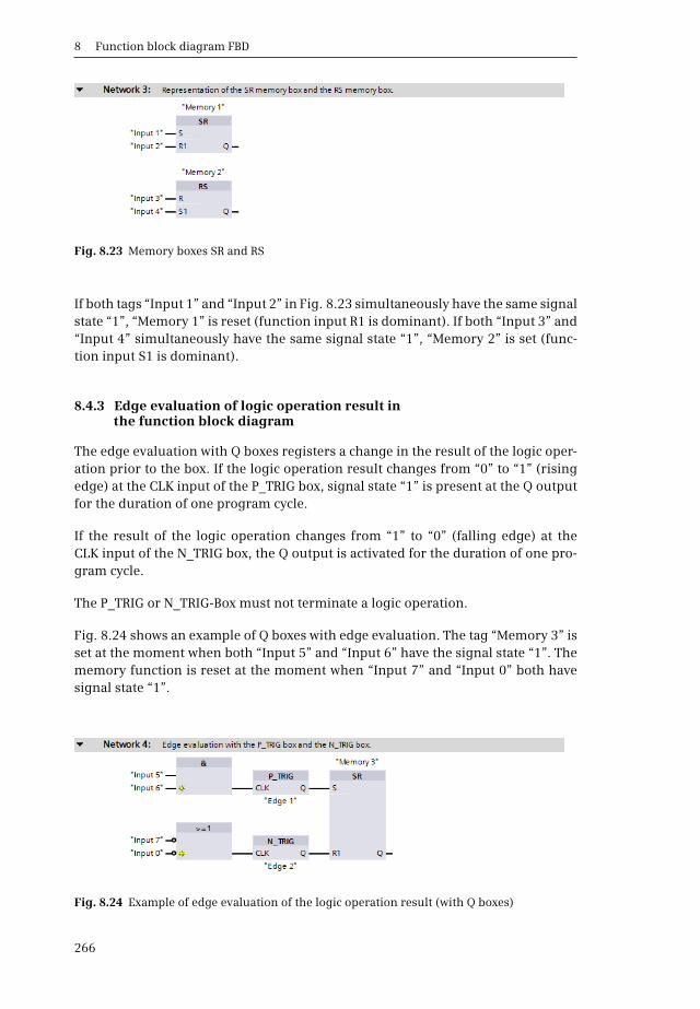
8 Function block diagram FBD
266
If both tags “Input 1” and “Input 2” in Fig. 8.23 simultaneously have the same signalstate “1”, “Memory 1” is reset (function input R1 is dominant). If both “Input 3” and“Input 4” simultaneously have the same signal state “1”, “Memory 2” is set (func-tion input S1 is dominant).
8.4.3 Edge evaluation of logic operation result in the function block diagram
The edge evaluation with Q boxes registers a change in the result of the logic oper-ation prior to the box. If the logic operation result changes from “0” to “1” (risingedge) at the CLK input of the P_TRIG box, signal state “1” is present at the Q outputfor the duration of one program cycle.
If the result of the logic operation changes from “1” to “0” (falling edge) at theCLK input of the N_TRIG box, the Q output is activated for the duration of one pro-gram cycle.
The P_TRIG or N_TRIG-Box must not terminate a logic operation.
Fig. 8.24 shows an example of Q boxes with edge evaluation. The tag “Memory 3” isset at the moment when both “Input 5” and “Input 6” have the signal state “1”. Thememory function is reset at the moment when “Input 7” and “Input 0” both havesignal state “1”.
Fig. 8.23 Memory boxes SR and RS
Fig. 8.24 Example of edge evaluation of the logic operation result (with Q boxes)
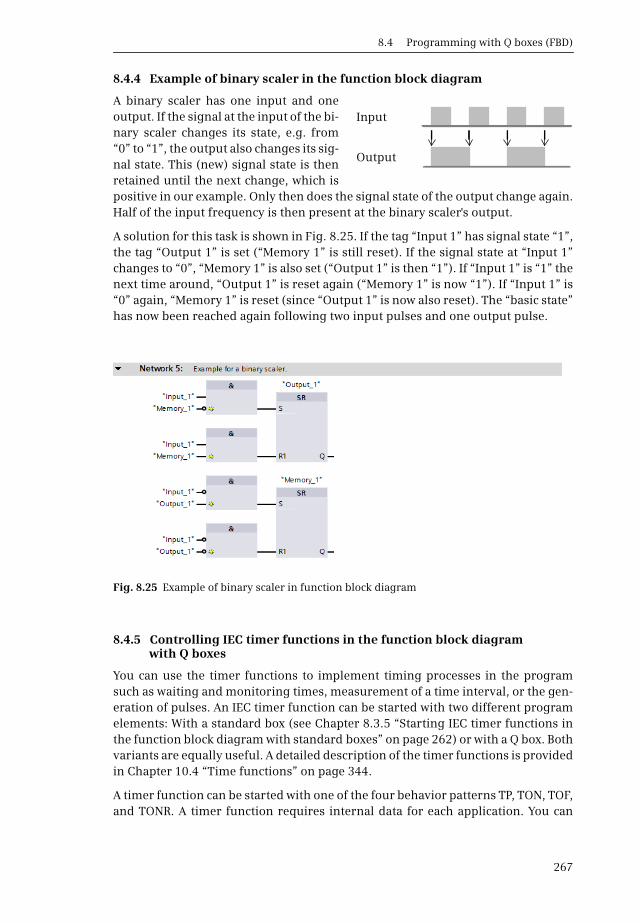
8.4 Programming with Q boxes (FBD)
267
8.4.4 Example of binary scaler in the function block diagram
A binary scaler has one input and oneoutput. If the signal at the input of the bi-nary scaler changes its state, e.g. from“0” to “1”, the output also changes its sig-nal state. This (new) signal state is thenretained until the next change, which ispositive in our example. Only then does the signal state of the output change again.Half of the input frequency is then present at the binary scaler's output.
A solution for this task is shown in Fig. 8.25. If the tag “Input 1” has signal state “1”,the tag “Output 1” is set (“Memory 1” is still reset). If the signal state at “Input 1”changes to “0”, “Memory 1” is also set (“Output 1” is then “1”). If “Input 1” is “1” thenext time around, “Output 1” is reset again (“Memory 1” is now “1”). If “Input 1” is“0” again, “Memory 1” is reset (since “Output 1” is now also reset). The “basic state”has now been reached again following two input pulses and one output pulse.
8.4.5 Controlling IEC timer functions in the function block diagram with Q boxes
You can use the timer functions to implement timing processes in the programsuch as waiting and monitoring times, measurement of a time interval, or the gen-eration of pulses. An IEC timer function can be started with two different programelements: With a standard box (see Chapter 8.3.5 “Starting IEC timer functions inthe function block diagram with standard boxes” on page 262) or with a Q box. Bothvariants are equally useful. A detailed description of the timer functions is providedin Chapter 10.4 “Time functions” on page 344.
A timer function can be started with one of the four behavior patterns TP, TON, TOF,and TONR. A timer function requires internal data for each application. You can
Fig. 8.25 Example of binary scaler in function block diagram
Input
Output
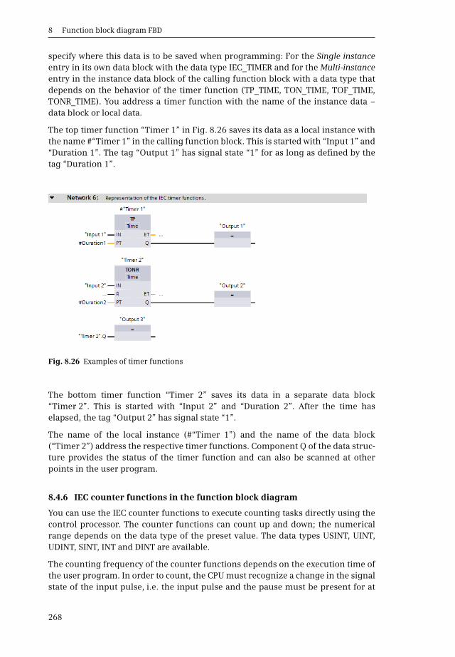
8 Function block diagram FBD
268
specify where this data is to be saved when programming: For the Single instanceentry in its own data block with the data type IEC_TIMER and for the Multi-instanceentry in the instance data block of the calling function block with a data type thatdepends on the behavior of the timer function (TP_TIME, TON_TIME, TOF_TIME,TONR_TIME). You address a timer function with the name of the instance data –data block or local data.
The top timer function “Timer 1” in Fig. 8.26 saves its data as a local instance withthe name #“Timer 1” in the calling function block. This is started with “Input 1” and“Duration 1”. The tag “Output 1” has signal state “1” for as long as defined by thetag “Duration 1”.
The bottom timer function “Timer 2” saves its data in a separate data block“Timer 2”. This is started with “Input 2” and “Duration 2”. After the time haselapsed, the tag “Output 2” has signal state “1”.
The name of the local instance (#“Timer 1”) and the name of the data block(“Timer 2”) address the respective timer functions. Component Q of the data struc-ture provides the status of the timer function and can also be scanned at otherpoints in the user program.
8.4.6 IEC counter functions in the function block diagram
You can use the IEC counter functions to execute counting tasks directly using thecontrol processor. The counter functions can count up and down; the numericalrange depends on the data type of the preset value. The data types USINT, UINT,UDINT, SINT, INT and DINT are available.
The counting frequency of the counter functions depends on the execution time ofthe user program. In order to count, the CPU must recognize a change in the signalstate of the input pulse, i.e. the input pulse and the pause must be present for at
Fig. 8.26 Examples of timer functions
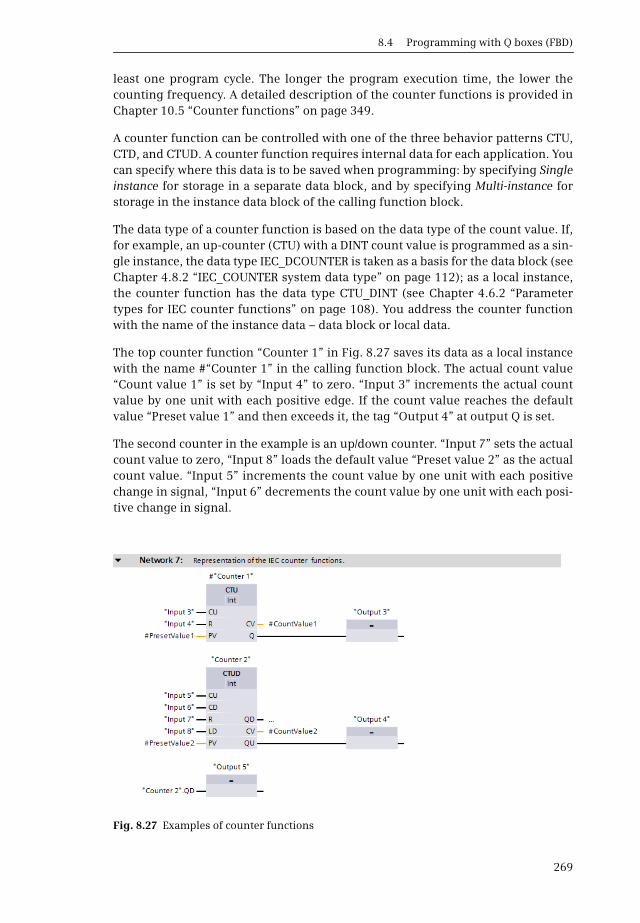
8.4 Programming with Q boxes (FBD)
269
least one program cycle. The longer the program execution time, the lower thecounting frequency. A detailed description of the counter functions is provided inChapter 10.5 “Counter functions” on page 349.
A counter function can be controlled with one of the three behavior patterns CTU,CTD, and CTUD. A counter function requires internal data for each application. Youcan specify where this data is to be saved when programming: by specifying Singleinstance for storage in a separate data block, and by specifying Multi-instance forstorage in the instance data block of the calling function block.
The data type of a counter function is based on the data type of the count value. If,for example, an up-counter (CTU) with a DINT count value is programmed as a sin-gle instance, the data type IEC_DCOUNTER is taken as a basis for the data block (seeChapter 4.8.2 “IEC_COUNTER system data type” on page 112); as a local instance,the counter function has the data type CTU_DINT (see Chapter 4.6.2 “Parametertypes for IEC counter functions” on page 108). You address the counter functionwith the name of the instance data – data block or local data.
The top counter function “Counter 1” in Fig. 8.27 saves its data as a local instancewith the name #“Counter 1” in the calling function block. The actual count value“Count value 1” is set by “Input 4” to zero. “Input 3” increments the actual countvalue by one unit with each positive edge. If the count value reaches the defaultvalue “Preset value 1” and then exceeds it, the tag “Output 4” at output Q is set.
The second counter in the example is an up/down counter. “Input 7” sets the actualcount value to zero, “Input 8” loads the default value “Preset value 2” as the actualcount value. “Input 5” increments the count value by one unit with each positivechange in signal, “Input 6” decrements the count value by one unit with each posi-tive change in signal.
Fig. 8.27 Examples of counter functions

8 Function block diagram FBD
270
The QU output has the signal state “1” if the actual count value at the CV output isequal to or greater than the default value at the PV input. The QD output has the sig-nal state “1” if the actual count value is zero or less than zero.
The lower QU output can be further connected directly. In the example, it is used tocontrol the tag “Output 5”. The QD output cannot be supplied, but can be scannedindirectly via the corresponding component QD of the counter structure. (For theQU output, this would be the component QU.)
The name of the local instance (#“Counter 1”) and the name of the data block(“Counter 2”) address the respective counter function. In the example, “Counter 2”has its own data block, and the QD output is scanned with the name “Counter 2”.QD.The result of the query can be connected further, e.g. to control an assignment.
8.5 Programming with EN/ENO boxes (FBD)
EN/ENO boxes have an enabling input EN and an enabling output ENO. The enablinginput can be used to suppress processing of the box. If an error occurs while the boxis being processed, this is displayed at the enabling output.
A detailed description of the functions with EN/ENO boxes can be found in the cor-responding sections. Programming of the EN/ENO boxes in the function block dia-gram is the primary focus here. Fig. 8.28 provides an overview of the functions im-plemented with EN/ENO boxes.
The parameters of the EN/ENO boxes must all be connected. The enabling input ENand the enabling output ENO are not parameters of the box function. They are usedfor processing boxes, and are added by the program editor to the box function.
A detailed description of EN and ENO and how the EN/ENO mechanism can be usedwith self-created blocks can be found in Chapter 12.4.1 “EN/ENO mechanism withLAD and FBD” on page 418.
The block calls in the function block diagram which are also shown as EN/ENO boxesare described in Chapter 8.6.5 “Block call functions in the function block diagram”on page 282.
8.5.1 Positioning of EN/ENO boxes in the function block diagram
Fig. 8.29 uses the MOVE function to show the positioning of EN/ENO boxes in a logicoperation. An EN/ENO box can be positioned on its own in a network, with or with-out connection of the EN input or the ENO output.
The ENO output can be connected to the EN input of the following box. A binary tagat the EN input of the first box can be used to switch processing of the complete boxseries on and off. The ENO output of the last box indicates by means of signal state“1” that the complete sequence has been executed without errors.
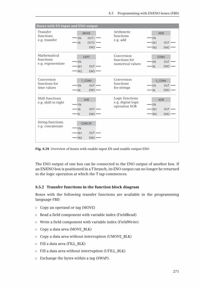
8.5 Programming with EN/ENO boxes (FBD)
271
The ENO output of one box can be connected to the ENO output of another box. Ifan EN/ENO box is positioned in a T branch, its ENO output can no longer be returnedto the logic operation at which the T tap commences.
8.5.2 Transfer functions in the function block diagram
Boxes with the following transfer functions are available in the programminglanguage FBD:
b Copy an operand or tag (MOVE)
b Read a field component with variable index (FieldRead)
b Write a field component with variable index (FieldWrite)
b Copy a data area (MOVE_BLK)
b Copy a data area without interruption (UMOVE_BLK)
b Fill a data area (FILL_BLK)
b Fill a data area without interruption (UFILL_BLK)
b Exchange the bytes within a tag (SWAP).
Fig. 8.28 Overview of boxes with enable input EN and enable output ENO
MOVE
SHR
CONV
T_CONV S_CONV
EXPT
CONCAT
ADD
XOR
EN
EN
EN
EN EN
EN
EN
EN
EN
IN
IN
N
IN
IN IN
IN1
IN1
IN2
IN2
IN1
IN1
IN2
IN2
OUT1
ENO
OUT
OUT OUT
ENO
ENO
ENO
ENO
OUT2
OUT
ENO
ENO
ENO ENO
OUT
OUT
OUT
OUT
Transfer functionse.g. transfer
Shift functions e.g. shift to right
Conversion functions for numerical values
Conversion functions for time values
Conversion functions for strings
Arithmetic functions e.g. add
Logic functions e.g. digital logic operation XOR
Mathematical functions e.g. exponentiate
String functions e.g. concatenate
Boxes with EN input and ENO output
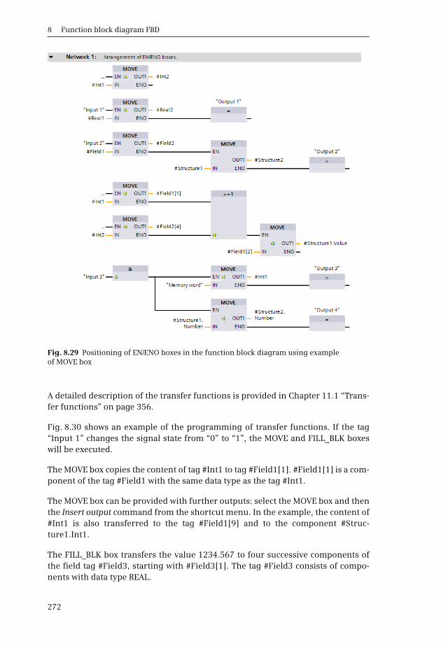
8 Function block diagram FBD
272
A detailed description of the transfer functions is provided in Chapter 11.1 “Trans-fer functions” on page 356.
Fig. 8.30 shows an example of the programming of transfer functions. If the tag“Input 1” changes the signal state from “0” to “1”, the MOVE and FILL_BLK boxeswill be executed.
The MOVE box copies the content of tag #Int1 to tag #Field1[1]. #Field1[1] is a com-ponent of the tag #Field1 with the same data type as the tag #Int1.
The MOVE box can be provided with further outputs: select the MOVE box and thenthe Insert output command from the shortcut menu. In the example, the content of#Int1 is also transferred to the tag #Field1[9] and to the component #Struc-ture1.Int1.
The FILL_BLK box transfers the value 1234.567 to four successive components ofthe field tag #Field3, starting with #Field3[1]. The tag #Field3 consists of compo-nents with data type REAL.
Fig. 8.29 Positioning of EN/ENO boxes in the function block diagram using example of MOVE box
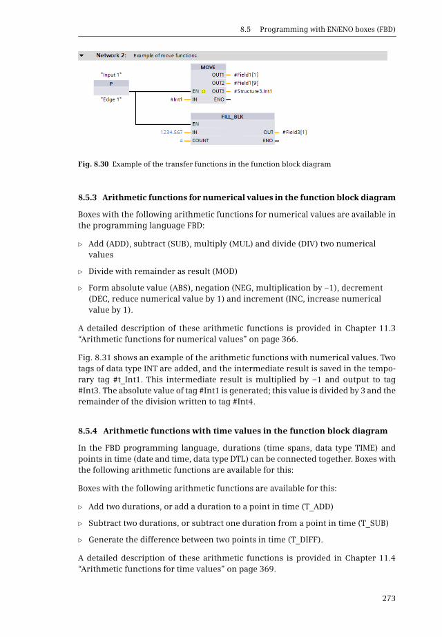
8.5 Programming with EN/ENO boxes (FBD)
273
8.5.3 Arithmetic functions for numerical values in the function block diagram
Boxes with the following arithmetic functions for numerical values are available inthe programming language FBD:
b Add (ADD), subtract (SUB), multiply (MUL) and divide (DIV) two numerical values
b Divide with remainder as result (MOD)
b Form absolute value (ABS), negation (NEG, multiplication by –1), decrement (DEC, reduce numerical value by 1) and increment (INC, increase numerical value by 1).
A detailed description of these arithmetic functions is provided in Chapter 11.3“Arithmetic functions for numerical values” on page 366.
Fig. 8.31 shows an example of the arithmetic functions with numerical values. Twotags of data type INT are added, and the intermediate result is saved in the tempo-rary tag #t_Int1. This intermediate result is multiplied by –1 and output to tag#Int3. The absolute value of tag #Int1 is generated; this value is divided by 3 and theremainder of the division written to tag #Int4.
8.5.4 Arithmetic functions with time values in the function block diagram
In the FBD programming language, durations (time spans, data type TIME) andpoints in time (date and time, data type DTL) can be connected together. Boxes withthe following arithmetic functions are available for this:
Boxes with the following arithmetic functions are available for this:
b Add two durations, or add a duration to a point in time (T_ADD)
b Subtract two durations, or subtract one duration from a point in time (T_SUB)
b Generate the difference between two points in time (T_DIFF).
A detailed description of these arithmetic functions is provided in Chapter 11.4“Arithmetic functions for time values” on page 369.
Fig. 8.30 Example of the transfer functions in the function block diagram
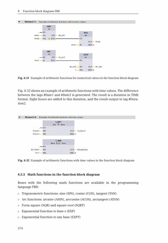
8 Function block diagram FBD
274
Fig. 8.32 shows an example of arithmetic functions with time values. The differencebetween the tags #Date1 and #Date2 is generated. The result is a duration in TIMEformat. Eight hours are added to this duration, and the result output to tag #Dura-tion2.
8.5.5 Math functions in the function block diagram
Boxes with the following math functions are available in the programminglanguage FBD:
b Trigonometric functions: sine (SIN), cosine (COS), tangent (TAN)
b Arc functions: arcsine (ASIN), arccosine (ACOS), arctangent (ATAN)
b Form square (SQR) and square root (SQRT)
b Exponential function to base e (EXP)
b Exponential function to any base (EXPT)
Fig. 8.31 Example of arithmetic functions for numerical values in the function block diagram
Fig. 8.32 Example of arithmetic functions with time values in the function block diagram

8.5 Programming with EN/ENO boxes (FBD)
275
b Natural logarithm (LN)
b Extract decimal places (FRAC)
A detailed description of these math functions is provided in Chapter 11.5 “Mathe-matical functions” on page 372.
Fig. 8.33 shows an example of the math functions.
The tag #c is calculated according to the equation. The square of #ais formed first. When inputting tag names – which can also be keywords (in theinput, “a” can also stand for “output”) or which can have the same name both locallyand globally – the tag must be labeled accordingly: for a local tag with a precedingnumber sign (#), for a global tag with the name in quotation marks, and for an oper-and (absolute address) with a preceding percent sign (%).
In the example, the squares of #a and #b are stored temporarily and added. #t_Real1is used again for the buffer. The result of the square root extraction is saved in thetag #c.
8.5.6 Conversion functions in the function block diagram
Boxes with the following conversion functions are available in the programminglanguage FBD:
b CONV (conversion of BYTE, WORD, DWORD, SINT, INT, DINT, USINT,UINT, UDINT, REAL, LREAL, BCD16, BCD32)
b ROUND, FLOOR, CEIL, TRUNC (conversion of REAL, LREAL into SINT,INT, DINT, USINT, UINT, UDINT, REAL, LREAL)
b SCALE_X, NORM_X (scaling and standardization)
b T_CONV (conversion of TIME into DINT and vice versa)
b S_CONV, STRG_VAL, VAL_STRG (conversion of SINT, INT, DINT, USINT,UINT, UDINT, REAL into STRING and vice versa)
Fig. 8.33 Example of math functions in the function block diagram
c a2 b2+=

8 Function block diagram FBD
276
A detailed description of the conversion functions is provided in Chapter 11.6 “Con-version functions (Conversion of data type)” on page 376.
Fig. 8.34 shows an example of the conversion functions.
The conversion function CONV is used to convert a 7-digit BCD number into a DINTformat number and subsequently into REAL format (tag #Real2). The value of#Real2 is divided by 107 and converted into a fixed-point number between the limitsof –150 and +250.
8.5.7 Shift functions in the function block diagram
Boxes with the following shift functions are available in the programminglanguage FBD:
b Shift to right (SHR) and left (SHL)
b Rotate to right (ROR) and left (ROL)
A detailed description of the shift functions is provided in Chapter 11.7 “Shift func-tions” on page 389.
Fig. 8.34 Example of conversion functions in the function block diagram
Fig. 8.35 Example of shift functions in the function block diagram

8.5 Programming with EN/ENO boxes (FBD)
277
Fig. 8.35 shows an example of the shift functions. The content of tag #Int2 is shiftedthree places to the right and output to tag #Int3. Shifting of fixed-point numbersone place to the right is equivalent to a division by two. In the example, tag #Int2 isdivided by eight (23) and the rounded-off result output to tag #Int3.
8.5.8 Logic functions in the function block diagram
Boxes with the following logic functions are available in the programminglanguage FBD:
b Digital logic operations AND, OR and XOR
b Invert (INV)
b Code bit (DECO) and set bit number (ENCO)
b Selection functions (SEL, MUX), minimum and maximum selection (MIN, MAX), limiter (LIMIT)
A detailed description of the logic functions is provided in Chapter 11.7 “Shift func-tions” on page 389.
Fig. 8.36 shows an example of the logic functions.
The MUX function is used to select the components whose number is present in thetag #Selection from the first four components of field tag #Field4. If, for example,the tag #Selection has a value of 3, the tag #Field4[3] will be selected.
If the value of #Selection is not between 1 and 4, the value of the tag #Real4 is usedas a substitute. The result of the selection is limited to the range between –375 and+1200 and output to #Real1.
The MUX box has been extended in the example by two inputs: select the box whenprogramming and then the Insert input command from the shortcut menu.
Fig. 8.36 Example of logic functions in the function block diagram
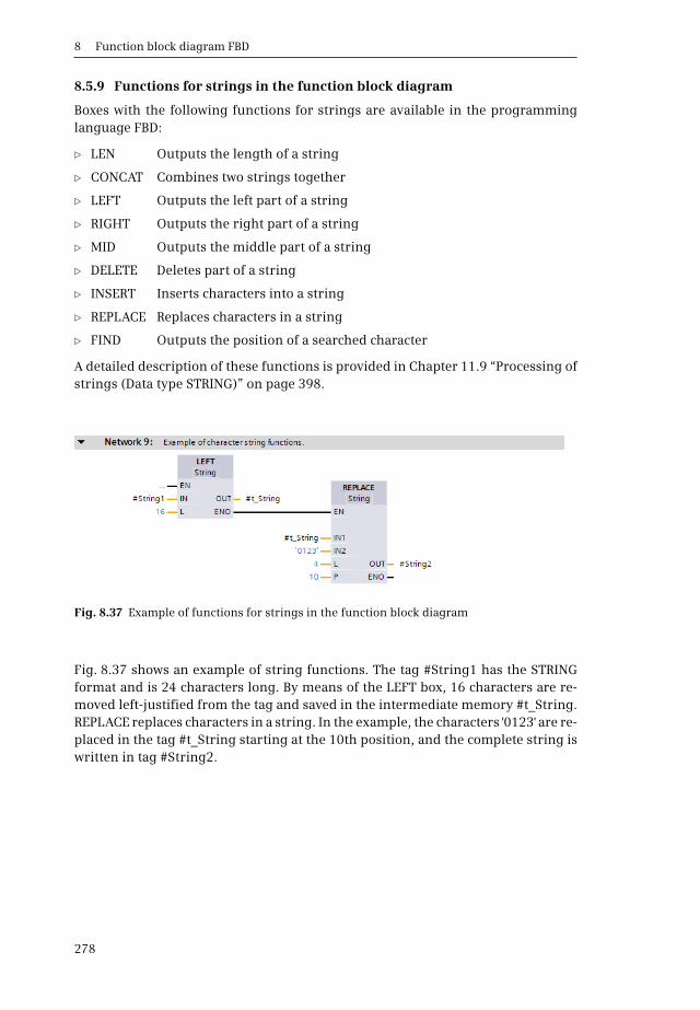
8 Function block diagram FBD
278
8.5.9 Functions for strings in the function block diagram
Boxes with the following functions for strings are available in the programminglanguage FBD:
b LEN Outputs the length of a string
b CONCAT Combines two strings together
b LEFT Outputs the left part of a string
b RIGHT Outputs the right part of a string
b MID Outputs the middle part of a string
b DELETE Deletes part of a string
b INSERT Inserts characters into a string
b REPLACE Replaces characters in a string
b FIND Outputs the position of a searched character
A detailed description of these functions is provided in Chapter 11.9 “Processing ofstrings (Data type STRING)” on page 398.
Fig. 8.37 shows an example of string functions. The tag #String1 has the STRINGformat and is 24 characters long. By means of the LEFT box, 16 characters are re-moved left-justified from the tag and saved in the intermediate memory #t_String.REPLACE replaces characters in a string. In the example, the characters '0123' are re-placed in the tag #t_String starting at the 10th position, and the complete string iswritten in tag #String2.
Fig. 8.37 Example of functions for strings in the function block diagram
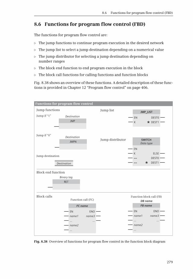
8.6 Functions for program flow control (FBD)
279
8.6 Functions for program flow control (FBD)
The functions for program flow control are:
b The jump functions to continue program execution in the desired network
b The jump list to select a jump destination depending on a numerical value
b The jump distributor for selecting a jump destination depending on number ranges
b The block end function to end program execution in the block
b The block call functions for calling functions and function blocks
Fig. 8.38 shows an overview of these functions. A detailed description of these func-tions is provided in Chapter 12 “Program flow control” on page 406.
Fig. 8.38 Overview of functions for program flow control in the function block diagram
JMP
JMPN
RET
Binary tag
Destination
DestinationSWITCH
Data type
EN
K
==
== DEST1
ELSE
DEST0
*
Jump functions Jump list
Jump distributor
Block callsFunction call (FC)
Function block call (FB)
Block end function
Functions for program flow control
FC name
JMP_LIST
EN
EN
name1
K
...
name2
...
name3
DEST1
...
ENO
DEST0
DB name
FB name
EN
name1
...
name2
...
name3
...
ENO
Jump if “0”
Jump if “1”
Jump destination
Destination
*

8 Function block diagram FBD
280
8.6.1 Jump functions in the function block diagram
A JMP or JMPN jump function is used to exit the linear processing in a block and –depending on the result of preceding logic operation – continue this processing inanother network in the block. If there is no preceding logic operation for JMP, thejump function is always performed. To program a jump function, drag the JMP orJMPN function from the program elements catalog under Basic instructions > Pro-gram control operations to the working area.
The jump label above the jump function defines the jump destination, which mustbe at the beginning of a network. To program the jump destination, drag the Labelfunction from the program elements catalog under Basic instructions > Programcontrol operations to the working area.
Fig. 8.39 shows a jump function using a program loop as an example. In a #Currentdata field with 16 components from #Current[0] to #Current[15], the maximumvalue is searched for. The tags #Index and #MaxValue are initialized with the value0. A comparison function in the program loop compares the value of #MaxValuewith the value of #Current[#Index]. If #MaxValue is less than #Current[#Index], it isoverwritten with the larger value of #Current[#Index]. #Index is then increased by+1. As long as #Index is less than or equal to 15, it jumps to the beginning of the pro-gram loop (to the jump destination MaxSearch) and the program part runs again.
Fig. 8.39 Example of a program loop with conditional jump
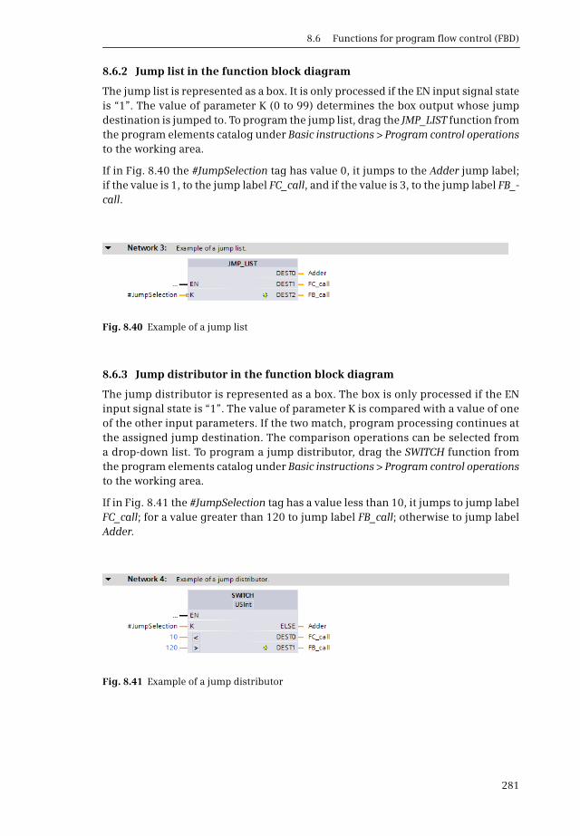
8.6 Functions for program flow control (FBD)
281
8.6.2 Jump list in the function block diagram
The jump list is represented as a box. It is only processed if the EN input signal stateis “1”. The value of parameter K (0 to 99) determines the box output whose jumpdestination is jumped to. To program the jump list, drag the JMP_LIST function fromthe program elements catalog under Basic instructions > Program control operationsto the working area.
If in Fig. 8.40 the #JumpSelection tag has value 0, it jumps to the Adder jump label;if the value is 1, to the jump label FC_call, and if the value is 3, to the jump label FB_-call.
8.6.3 Jump distributor in the function block diagram
The jump distributor is represented as a box. The box is only processed if the ENinput signal state is “1”. The value of parameter K is compared with a value of oneof the other input parameters. If the two match, program processing continues atthe assigned jump destination. The comparison operations can be selected froma drop-down list. To program a jump distributor, drag the SWITCH function fromthe program elements catalog under Basic instructions > Program control operationsto the working area.
If in Fig. 8.41 the #JumpSelection tag has a value less than 10, it jumps to jump labelFC_call; for a value greater than 120 to jump label FB_call; otherwise to jump labelAdder.
Fig. 8.40 Example of a jump list
Fig. 8.41 Example of a jump distributor
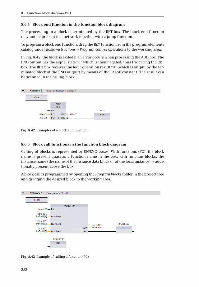
8 Function block diagram FBD
282
8.6.4 Block end function in the function block diagram
The processing in a block is terminated by the RET box. The block end functionmay not be present in a network together with a jump function.
To program a block end function, drag the RET function from the program elementscatalog under Basic instructions > Program control operations to the working area.
In Fig. 8.42, the block is exited if an error occurs when processing the ADD box. TheENO output has the signal state “0” which is then negated, thus triggering the RETbox. The RET box receives the logic operation result “0” (which is output by the ter-minated block at the ENO output) by means of the FALSE constant. The result canbe scanned in the calling block.
8.6.5 Block call functions in the function block diagram
Calling of blocks is represented by EN/ENO boxes. With functions (FC), the blockname is present quasi as a function name in the box; with function blocks, theinstance name (the name of the instance data block or of the local instance) is addi-tionally present above the box.
A block call is programmed by opening the Program blocks folder in the project treeand dragging the desired block to the working area.
Fig. 8.42 Examples of a block end function
Fig. 8.43 Example of calling a function (FC)
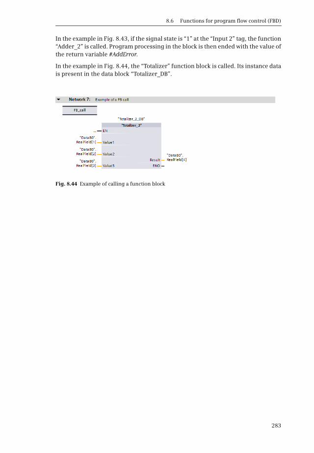
8.6 Functions for program flow control (FBD)
283
In the example in Fig. 8.43, if the signal state is “1” at the “Input 2” tag, the function“Adder_2” is called. Program processing in the block is then ended with the value ofthe return variable #AddError.
In the example in Fig. 8.44, the “Totalizer” function block is called. Its instance datais present in the data block “Totalizer_DB”.
Fig. 8.44 Example of calling a function block
9 Structured Control Language SCL
284
9 Structured Control Language SCL
9.1 Introduction to programming with SCL
This chapter describes programming with Structured Control Language (SCL); ituses examples to show how the program functions are represented in SCL. You canfind a description of the individual functions, e.g. comparison functions, in Chap-ters 10 “Basic functions” on page 328, 11 “Digital functions” on page 355, and 12“Program flow control” on page 406.
Use of the program and symbol editor, which generally applies to all programminglanguages, is described in Chapter 6 “Program editor” on page 178.
SCL is used to program the contents of blocks. What blocks are, and how they arecreated, is described in Chapters 5.3.1 “Block types” on page 125 and 6.3 “Program-ming a code block” on page 183.
9.1.1 Programming with SCL in general
You use SCL to program the control function of the programmable controller – theuser program or control program. The user program is organized in different typesof blocks.
Fig. 9.1 shows the SCL program for a FIFO register. With a rising edge at #Write, thisblock writes the value present at the #Input parameter into a FIFO register. With arising edge at #Read, the value at #Output is output again. The values are read outin the order in which they were written into the register (FIFO, first in first out). Theregister can be emptied using #Delete. The two displays #Full and #Empty show thestatus of the register (#Full and #Empty are each set following writing or reading).The block works with a write pointer and a read pointer.
The program editor constructs an SCL program line by line. You commence with thefirst statement in the first line. Each SCL statement is concluded by a semicolon.You can write several statements in one line, or one statement can occupy severallines.
You can make the SCL program clearer and easier to read by using comments andempty lines. Comments and empty lines have no influence on the function of theSCL program.
Line comments commence with two slashes and terminate at the end of the line.Block comments commence with left parenthesis and asterisk, can extend over sev-eral lines, and terminate with asterisk and right parenthesis.
In order to program an SCL statement, use the keyboard to enter the statements ina line of the input field. Dragging the statement with the mouse from the program

9.1 Introduction to programming with SCL
285
elements catalog is of advantage with SCL if you import functions with a parameterlist into your program. To call self-created blocks, drag the blocks from the Programblocks folder in the project tree into a line.
Fig. 9.1 Example of a block with SCL program

9 Structured Control Language SCL
286
9.1.2 SCL statements and operators
The SCL program consists of a sequence of individual STL statements. Fig. 9.2shows which types of SCL statements exist.
The simplest case with a Value assignment is that the content of a tag is transferredto another tag. Control statements guide program execution, for example with pro-gram loops. Block calls are used to continue program execution in the called block.
Operators
An expression represents a value. It can comprise a single address (a single tag) orseveral addresses (tags) which are linked by operators.
Example: “a + b” is an expression; “a” and “b” are addresses, “+” is the operator.
The sequence of logic operations is defined by the priority of the operators and canbe controlled by parentheses. Mixing of expressions is permissible providing thedata types generated during calculation of the expression permit this.
SCL provides the operators specified in Table 9.1. Operators of equal priority areprocessed from the left to the right.
Table 9.1 Operators with SCL
Operation Name Operator Priority
Parentheses Left parenthesis, right parenthesis (, ) 1
Arithmetic Power ** 2
Unary plus, unary minus (sign) +, – 3
Multiplication, division *, /, DIV, MOD 4
Addition, subtraction +, – 5
Comparison Less than, less than-equal to, greater than, greater than-equal to
<, <=, >, >= 6
Equal to, not equal to =, <> 7
Binary logic operation Negation (unary) NOT 3
AND logic operation AND, & 8
Exclusive OR XOR 9
OR logic operation OR 10
Assignment Assignment := 11
“Unary” means that this operator has a fixed assignment to an address
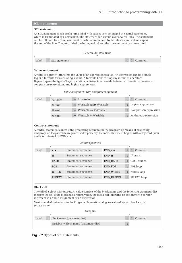
9.1 Introduction to programming with SCL
287
Fig. 9.2 Types of SCL statements
Label
Label
Label
Label
SCL statement
Variable
xxx
IF
CASE
FOR
WHILE
REPEAT
#Result
#Result
#Result
Statement sequence
Block name (parameter list)
Statement sequence
Variable := Block name (parameter list)
Statement sequence
Statement sequence
Statement sequence
Statement sequence
Expression
END_xxx
END_IF
END_CASE
END_FOR
END_WHILE
END_REPEAT
#Variable #VariableAND
#Variable #Variable>=
#Variable #Variable+
:=
:=
:=
:=
;
;
;
;
;
;
;
;
;
;
;
;
;
//
//
//
//
:
:
:
:
General SCL statement
Value assignment with assignment operator
Block call
Logical expression
IF branch
CASE branch
FOR loop
WHILE loop
REPEAT loop
Comparison expression
Arithmetic expression
Comment
Comment
Comment
Comment
SCL statement
Value assignment
Control statement
Block call
SCL statements
An SCL statement consists of a jump label with subsequent colon and the actual statement, which is terminated by a semicolon. The statement can extend over several lines. The statement can be followed by a (line) comment, which is commenced by two slashes and extends up to the end of the line. The jump label (including colon) and the line comment can be omitted.
A value assignment transfers the value of an expression to a tag. An expression can be a single tag or a formula for calculating a value. A formula links the tags by means of operators. Depending on the type of logic operation, a distinction is made between arithmetic expressions,comparison expressions, and logical expressions.
A control statement controls the processing sequence in the program by means of branching and program loops which are processed repeatedly. A control statement begins with a keyword (xxx) and is terminated by END_xxx.
The call of a block without return value consists of the block name and the following parameter list in parentheses. If the block has a return value, the block call following an assignment operator is present in a value assignment or an expression.
Most extended statements in the Program Elements catalog are calls of system blocks with return value.
Control statement

9 Structured Control Language SCL
288
Expressions
An expression is a formula for calculating a value and consists of addresses (tags)and operators. In the simplest case, an expression is an address, a tag, or a constant.A sign or a negation can also be included.
An expression can consist of addresses that are linked together by operators.Expressions can also be linked by operators. Expression can therefore have a verycomplex structure. Parentheses can be used to control the processing sequence inan expression.
The result of an expression can be assigned to a tag or a block parameter or used asa condition in a control statement.
Expressions are distinguished according to the type of logic operation into arithme-tic expressions, comparison expressions, and logic expressions.
9.2 Programming binary logic operations with SCL
The binary logic operations are executed in SCL with logic expressions in conjunc-tion with binary tags or expressions which deliver a binary result. The binary oper-ations can be “nested” using parentheses and thus influence the processing se-quence (Table 9.2).
9.2.1 Scanning for signal states “1” and “0”
The scanning of a binary operand in SCL is always the direct scanning of the statusof the binary operand. This corresponds to scanning for signal state “1”. If scanningfor signal state “0” is required for the program function, one uses the NOT operatorin order to negate the result of scan. NOT can also be used to negate the result ofbinary expressions.
Fig. 9.3 shows a sensor connected to the programmable controller which is scannedfor signal state “1” (left-hand side) and for signal state “0” (right-hand side). Theresult of the scan is connected directly to a contactor.
Table 9.2 Binary logic operations with SCL
Operation Operand Function
&
AND
OR
XOR
Binary operand or binary expression
Binary operand or binary expression
Binary operand or binary expression
Binary operand or binary expression
Scan for signal state “1” and combination according to AND logic operation
Scan for signal state “1” and combination according to AND logic operation
Scan for signal state “1” and combination according to OR logic operation
Scan for signal state “1” and combination according to exclusive OR logic operation
NOT – Negation of result of logic operation
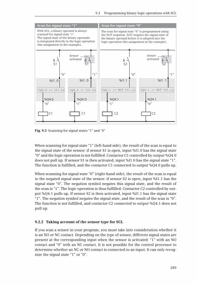
9.2 Programming binary logic operations with SCL
289
When scanning for signal state “1” (left-hand side), the result of the scan is equal tothe signal state of the sensor: if sensor S1 is open, input %I1.0 has the signal state“0” and the logic operation is not fulfilled. Contactor C1 controlled by output %Q4.0does not pull up. If sensor S1 is then activated, input %I1.0 has the signal state “1”.The function is fulfilled, and the contactor C1 connected to output %Q4.0 pulls up.
When scanning for signal state “0” (right-hand side), the result of the scan is equalto the negated signal state of the sensor: if sensor S2 is open, input %I1.1 has thesignal state “0”. The negation symbol negates this signal state, and the result ofthe scan is “1”. The logic operation is thus fulfilled. Contactor C2 controlled by out-put %Q4.1 pulls up. If sensor S2 is then activated, input %I1.1 has the signal state“1”. The negation symbol negates the signal state, and the result of the scan is “0”.The function is not fulfilled, and contactor C2 connected to output %Q4.1 does notpull up.
9.2.2 Taking account of the sensor type for SCL
If you scan a sensor in your program, you must take into consideration whether itis an NO or NC contact. Depending on the type of sensor, different signal states arepresent at the corresponding input when the sensor is activated: “1” with an NOcontact and “0” with an NC contact. It is not possible for the control processor todetermine whether an NC or NO contact is connected to an input. It can only recog-nize the signal state “1” or “0”.
Fig. 9.3 Scanning for signal states “1” and “0”
S1 S2
C1 C2C1 C2
S1 S2
%I1. 0 %I1. 1
%Q4.0 %Q4.1%Q4.0 %Q4.1
%I1. 0 %I1.1
“0”
“1”“1”
“1”“1”
“0”“0”
“0”
Scan for signal state “1” Scan for signal state “0”
Sensor activated
Sensor activated
%Q4.1 := NOT %I1.1; %Q4.1 := NOT %I1.1;%Q4.0 := %I1.0; %Q4.0 := %I1.0;
With SCL, a binary operand is always scanned for signal state “1”. The signal state of the binary operands is integrated directly in the logic operation (the assignment in the example).
The scan for signal state “0” is programmed using the NOT negation. NOT negates the signal state of the binary operand before it is adopted into the logic operation (the assignment in the example).

9 Structured Control Language SCL
290
If you write the program to obtain “1” when a sensor is activated in order to link itfurther, you must scan the input in different ways depending on the type of sensor.The negation NOT is available for this purpose. Direct scanning delivers “1” if thescanned input is also “1”. Together with the NOT negation, the scan then delivers“1” if the scanned input is “0”. In this manner you can also directly scan inputswhich are to execute activities when the signal state is “0” (“zero-active”) and con-nect the result of the scan further.
The example in Fig. 9.4 shows the programming dependent on the type of sensor.The AND function used is then fulfilled, i.e. the function result has signal state “1”
Fig. 9.4 Taking account of the sensor type for SCL
Neither sensor is activated
Neither sensor is activated
Both sensor is activated
Both sensor is activated
The contactor pulls up
S3
S5
S3
S5
S4
S6
S4
S6
C3
C4
C3
C4
%I1.2
%I1.4
%I1.2
%I1.4
%I1.3
%I1.5
%I1.3
%I1.5
%Q4.2
%Q4.3
%Q4.2
%Q4.3
“0”
“0” “0”
“0” “1”
“1”
“1”
“1”
“1”
“1”
“0”
“0”
Case 1: Both sensors are NO contacts
Case 2: The sensors are one NO contact and one NC contact
%Q4.3 := %I1.4 AND NOT %I1.5;%Q4.3 := %I1.4 AND NOT %I1.5;
%Q4.3 := %I1.4 AND %I1.5; %Q4.3 := %I1.4 AND %I1.5;
When actuated, an NO contact returns signal state “1”. If both sensors are actuated, both inputs have signal state “1” and a scan result of “1” for a direct scan. The AND function is thus fulfilled and the contactor at the output picks up."
The contactor pulls up
When actuated, an NC contact returns signal state “0”. If both sensors are actuated, the NO contact at the input has signal state “1” and the NC contact has signal state “0”. In order to get signal state “1” when the NC contact is actuated, the scan result must be negated. Then, if both sensors are actuated,the AND function is fulfilled and the contactor at the output picks up."
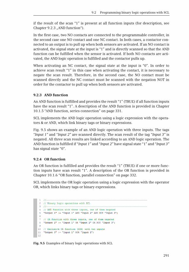
9.2 Programming binary logic operations with SCL
291
if the result of the scan “1” is present at all function inputs (for description, seeChapter 9.2.3 „AND function“).
In the first case, two NO contacts are connected to the programmable controller, inthe second case one NO contact and one NC contact. In both cases, a contactor con-nected to an output is to pull up when both sensors are activated. If an NO contact isactivated, the signal state at the input is “1” and is directly scanned so that the ANDfunction can be fulfilled when the sensor is activated. If both NO contacts are acti-vated, the AND logic operation is fulfilled and the contactor pulls up.
When activating an NC contact, the signal state at the input is “0”. In order toachieve scan result “1” in this case when activating the contact, it is necessary tonegate the scan result. Therefore, in the second case, the NO contact must bescanned directly and the NC contact must be scanned with the negation NOT inorder for the contactor to pull up when both sensors are activated.
9.2.3 AND function
An AND function is fulfilled and provides the result “1” (TRUE) if all function inputshave the scan result “1”. A description of the AND function is provided in Chapter10.1.5 “AND function, series connection” on page 331.
SCL implements the AND logic operation using a logic expression with the opera-tors & or AND, which link binary tags or binary expressions.
Fig. 9.5 shows an example of an AND logic operation with three inputs. The tags“Input 1” and “Input 2” are scanned directly. The scan result of the tag “Input 3” isnegated. All three scan results are linked according to an AND logic operation. TheAND function is fulfilled if “Input 1” and “Input 2” have signal state “1” and “Input 3”has signal state “0”.
9.2.4 OR function
An OR function is fulfilled and provides the result “1” (TRUE) if one or more func-tion inputs have scan result “1”. A description of the OR function is provided inChapter 10.1.6 “OR function, parallel connection” on page 332.
SCL implements the OR logic operation using a logic expression with the operatorOR, which links binary tags or binary expressions.
Fig. 9.5 Examples of binary logic operations with SCL

9 Structured Control Language SCL
292
Fig. 9.5 shows an example of an OR logic operation with three inputs. The tags“Input 1” and “Input 2” are scanned directly. The scan result of the tag “Input 3” isnegated. All three scan results are linked according to an OR logic operation. TheOR function is fulfilled if “Input 1” or “Input 2” has signal state “1” or “Input 3” hassignal state “0”.
9.2.5 Exclusive OR function
An exclusive OR function (antivalence function) is fulfilled and provides the result“1” (TRUE) if an odd number of function inputs have scan result “1”. A descriptionof the exclusive OR function is provided in Chapter 10.1.7 “Exclusive OR function,non-equivalence function” on page 333.
SCL implements the exclusive OR logic operation using a logic expression with theoperator XOR, which links binary tags or binary expressions.
Fig. 9.5 shows an example of an exclusive OR logic operation with two inputs. Thetags “Input 1” and “Input 2” are scanned directly. The scan results are linked accord-ing to an exclusive OR logic operation. The exclusive OR function is fulfilled (it sup-plies the value TRUE) if the signal states at “Input 1” and “Input 2” are different.
9.2.6 Combined binary logic operations
The AND, OR, and exclusive OR functions can be freely combined with one another.With SCL the operators have the following priority regarding execution: AND or &are executed before XOR, followed by OR. NOT is executed before the logic opera-tion operators.
Logic operations such as the ORing of AND functions do not require parentheses, asshown in the top example in Fig. 9.6. The first AND function is fulfilled if “Input 1”and “Input 2” have signal state “1”; the second AND function is fulfilled if “Input 3”and “Input 4” have signal state “1”. The tag “Output 4” is set if the first AND functionis fulfilled, or if the second AND function is fulfilled, or if both are fulfilled.
Fig. 9.6 Examples of combined binary logic operations with SCL

9.2 Programming binary logic operations with SCL
293
This logic operation does not require parentheses since the AND function is pro-cessed “before” the OR function because of its higher priority. The processing pri-ority can be influenced using parentheses. The expressions in the parentheses areprocessed first as it were. Parentheses can be nested.
Logic operations such as the ANDing of OR functions require parentheses, as shownin the following example in Fig. 9.6. The first OR function is fulfilled if “Input 1”, or“Input 2”, or both tags have signal state “1”; the second OR function is fulfilled if“Input 3”, or “Input 4”, or both tags have signal state “1”. Both OR functions are pres-ent in parentheses and their results of logic operation are linked according to anAND logic operation. The “Output 5” tag is set if both OR functions are fulfilled. Thelogic operation of exclusive OR functions according to an OR logic operation (lastexample in Fig. 9.6) also does not require parentheses. However, parentheses canbe used for reasons of clarity.
9.2.7 Negating the result of logic operation
The NOT operator negates the result of logic operation at any position in an logicoperation. Using the NOT operator it is possible in a simple manner to obtain:
b a NAND function (negated AND function, is fulfilled if at least one input has the result of scan “0”),
b a NOR function (negated OR function, is fulfilled if all inputs have the result of scan “0”), and
b an inclusive OR function (equivalence function, negated exclusive OR function, is fulfilled if an even number of inputs has the result of scan “1”).
Fig. 9.7 shows the negation of binary functions. The functions are present in paren-theses since they have a lower processing priority than NOT. First the result of thebinary function is generated in parentheses and then it is negated and assigned tothe output tag.
Fig. 9.7 Examples of the negation of binary functions

9 Structured Control Language SCL
294
9.3 Programming memory functions with SCL
The memory functions control binary tags such as outputs or bit memories. SCL hasvalue assignment as a memory function, which directly imports the result of logicoperation of the expression. The set and reset functions, which are only performedif the result of logic operation is “1”, can be emulated.
9.3.1 Value assignment of a binary tag
The value assignment assigns the result of logic operation of the expression to theright of the assignment operator to the binary tag on the left. The response of theassignment is described in Chapter 10.2.2 “Simple and negated coil, assignment”on page 334.
An example of a (binary) value assignment is shown in Fig. 9.8. Here, if the logicoperation is fulfilled and both tags “Input 1” and “Input 2” have the same signal sta-tus, the tag “Output 1” is set to signal state “1”, and if the logical operation is notfulfilled, to signal state “0”. If an assignment should be carried out negated, use thenegation NOT to negate the signal state of the expression.
9.3.2 Setting and resetting
With SCL, the setting and resetting on signal state “1” can be emulated, for examplewith a simple IF branch.
In Fig. 9.8, the tag “Output 3” is set to signal state “1” (value TRUE) if the AND logicoperation from “Input 3” and “Input 4” is fulfilled (supplies the value TRUE). If theAND logic operation is not fulfilled (if it has the value FALSE), “Output 3” is notaffected. Resetting of “Output 3” is carried out in a similar manner: If the expression“Input 5” OR “Input 6” is fulfilled (supplies the value TRUE), “Output 3” is set to sig-nal state “0” (FALSE). An expression which is not fulfilled does not influence “Output3”. Resetting is programmed following setting and is therefore “dominant”. If bothconditions are fulfilled, “Output 3” is reset or remains reset.
Fig. 9.8 Assigning, setting, and resetting with SCL
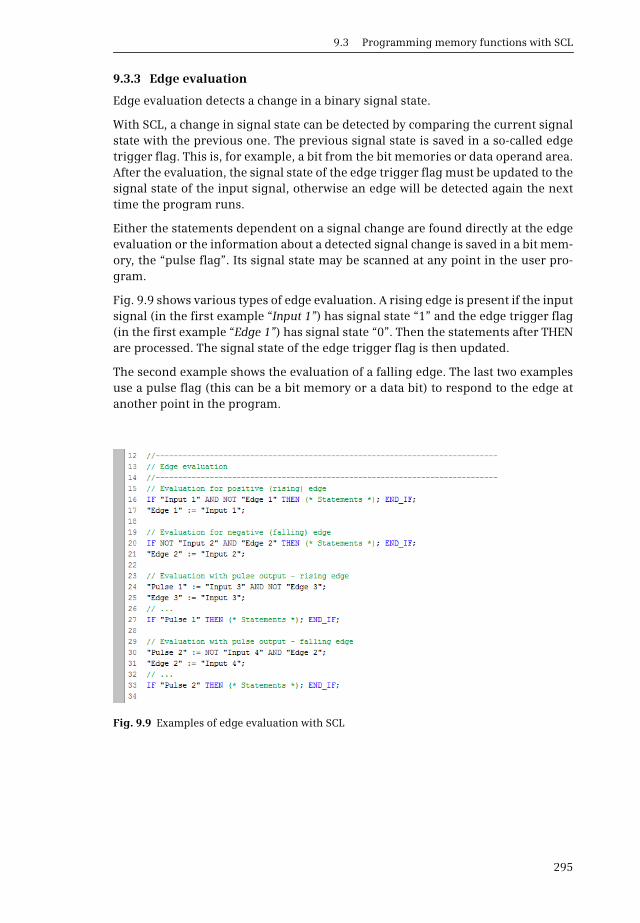
9.3 Programming memory functions with SCL
295
9.3.3 Edge evaluation
Edge evaluation detects a change in a binary signal state.
With SCL, a change in signal state can be detected by comparing the current signalstate with the previous one. The previous signal state is saved in a so-called edgetrigger flag. This is, for example, a bit from the bit memories or data operand area.After the evaluation, the signal state of the edge trigger flag must be updated to thesignal state of the input signal, otherwise an edge will be detected again the nexttime the program runs.
Either the statements dependent on a signal change are found directly at the edgeevaluation or the information about a detected signal change is saved in a bit mem-ory, the “pulse flag”. Its signal state may be scanned at any point in the user pro-gram.
Fig. 9.9 shows various types of edge evaluation. A rising edge is present if the inputsignal (in the first example “Input 1”) has signal state “1” and the edge trigger flag(in the first example “Edge 1”) has signal state “0”. Then the statements after THENare processed. The signal state of the edge trigger flag is then updated.
The second example shows the evaluation of a falling edge. The last two examplesuse a pulse flag (this can be a bit memory or a data bit) to respond to the edge atanother point in the program.
Fig. 9.9 Examples of edge evaluation with SCL
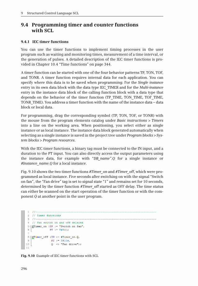
9 Structured Control Language SCL
296
9.4 Programming timer and counter functions with SCL
9.4.1 IEC timer functions
You can use the timer functions to implement timing processes in the userprogram such as waiting and monitoring times, measurement of a time interval, orthe generation of pulses. A detailed description of the IEC timer functions is pro-vided in Chapter 10.4 “Time functions” on page 344.
A timer function can be started with one of the four behavior patterns TP, TON, TOF,and TONR. A timer function requires internal data for each application. You canspecify where this data is to be saved when programming: For the Single instanceentry in its own data block with the data type IEC_TIMER and for the Multi-instanceentry in the instance data block of the calling function block with a data type thatdepends on the behavior of the timer function (TP_TIME, TON_TIME, TOF_TIME,TONR_TIME). You address a timer function with the name of the instance data – datablock or local data.
For programming, drag the corresponding symbol (TP, TON, TOF, or TONR) withthe mouse from the program elements catalog under Basic instructions > Timersinto a line on the working area. When positioning, you select either as singleinstance or as local instance. The instance data block generated automatically whenselecting as a single instance is saved in the project tree under Program blocks > Sys-tem blocks > Program resources.
With the IEC timer functions, a binary tag must be connected to the IN input, and aduration to the PT input. You can also directly access the output parameters usingthe instance data, for example with “DB_name”.Q for a single instance or#Instance_name.Q for a local instance.
Fig. 9.10 shows the two timer functions #Timer_on and #Timer_off, which were pro-grammed as local instance. Five seconds after switching on with the signal “Switchon fan”, the “Fan drive” tag is set to signal state “1” and remains set for 10 seconds,determined by the timer function #Timer_off started as OFF delay. The time statuscan either be scanned on the start operation of the timer function or with the com-ponent Q at another point in the user program.
Fig. 9.10 Example of IEC timer functions with SCL
9.4 Programming timer and counter functions with SCL
297
9.4.2 IEC counter functions
A counter function implements counting processes in the user program. A counterfunction can count up and down; the numerical range depends on the data type ofthe preset value. The data types USINT, UINT, UDINT, SINT, INT and DINT are avail-able.
The counting frequency of a counter function depends on the execution time of theuser program. In order to count, the CPU must recognize a change in the signalstate of the input pulse, i.e. the input pulse and the pause must be present for atleast one program cycle. The longer the program execution time, the lower thecounting frequency. A detailed description of the counter functions is provided inChapter 10.5 “Counter functions” on page 349.
A counter function can be controlled with one of the three behavior patterns CTU,CTD, and CTUD. A counter function requires internal data for each application. Youcan specify where this data is to be saved when programming: by specifying Singleinstance for storage in a separate data block, and by specifying Multi-instance forstorage in the instance data block of the calling function block.
The data type of a counter function is based on the data type of the count value. If,for example, an up-counter (CTU) with a DINT count value is programmed as a sin-gle instance, the data type IEC_DCOUNTER is taken as a basis for the data block (seeChapter 4.8.2 “IEC_COUNTER system data type” on page 112); as a local instance,the counter function has the data type CTU_DINT (see Chapter 4.6.2 “Parametertypes for IEC counter functions” on page 108). You address the counter functionwith the name of the instance data – data block or local data.
For programming, drag the corresponding symbol (CTU, CTD, or CTUD) with themouse from the program elements catalog under Basic instructions > Counters intoa line on the working area. When positioning, you select either as single instance oras local instance. The instance data block generated automatically when selectingas a single instance is saved in the project tree under Program blocks > System blocks> Program resources.
The data type of the counter function is set with a click on the instance name (thegreen box). With the IEC counter functions, a binary tag must be connected to atleast one counter input (CU or CD). Connection of the other function inputs and out-puts is optional. You can also directly access the output parameters using theinstance data, for example with “DB_name”.QD for a single instance or#Instance_name.QD for a local instance.
Fig. 9.11 shows the counter function #Lock_counter, which is called as a localinstance. It has saved its data in the instance data block of the calling function block.A component of the counter can be addressed globally with the name of theinstance and the component name, for example #LockCounter.CV. The exampleshows the passages through a lock, either forward or backward.

9 Structured Control Language SCL
298
9.5 Programming digital functions with SCL
The digital functions process digital values mainly with the data types for fixed-point and floating-point numbers.
The “simple” digital functions are implemented with SCL through the value assign-ment of an expression. When linking two values, the type of digital functiondepends on the operator used: comparison expression (comparison functions),arithmetic expression (arithmetic and mathematical functions), or logic expres-sion (e.g. word logic operations). The functions for data type conversion (conver-sion functions) and for shifting and rotating are available for manipulating just onevalue.
9.5.1 Transfer function, value assignment of a digital tag
The “simple” transfer function corresponds with SCL to the value assignment.
Both sides of the value assignment must have a “tolerable” data type that is eitherautomatically adapted (see Chapter 4.3.2 “Implicit data type conversion” on page
Fig. 9.11 Example of a counter function with SCL
Fig. 9.12 Examples of transfer and conversion functions with SCL
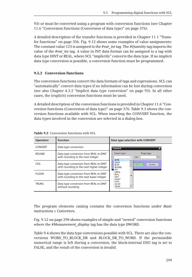
9.5 Programming digital functions with SCL
299
93) or must be converted using a program with conversion functions (see Chapter11.6 “Conversion functions (Conversion of data type)” on page 376).
A detailed description of the transfer functions is provided in Chapter 11.1 “Trans-fer functions” on page 356. Fig. 9.12 shows some examples of value assignments:The constant value 123 is assigned to the #var_int tag. The #Quantity tag imports thevalue of the #var_int tag. A value in INT data format can be assigned to a tag withdata type DINT or REAL, where SCL “implicitly” converts the data type. If no implicitdata type conversion is possible, a conversion function must be programmed.
9.5.2 Conversion functions
The conversion functions convert the data formats of tags and expressions. SCL can“automatically” convert data types if no information can be lost during conversion(see also Chapter 4.3.2 “Implicit data type conversion” on page 93). In all othercases, the (explicit) conversion functions must be used.
A detailed description of the conversion functions is provided in Chapter 11.6 “Con-version functions (Conversion of data type)” on page 376. Table 9.3 shows the con-version functions available with SCL. When inserting the CONVERT function, thedata types involved in the conversion are selected in a dialog box.
The program elements catalog contains the conversion functions under Basicinstructions > Converters.
Fig. 9.12 on page 298 shows examples of simple and “nested” conversion functionswhere the #Measurement_display tag has the data type DWORD.
Table 9.4 shows the data type conversions possible with SCL. There are also the con-versions WORD_TO_BLOCK_DB and BLOCK_DB_TO_WORD. If the permissiblenumerical range is left during a conversion, the block-internal ENO tag is set toFALSE, and the result of the conversion is invalid.
Table 9.3 Conversion functions with SCL
Operation Function Data type selection with CONVERT
CONVERT Data type conversion
ROUND Data type conversion from REAL to DINT with rounding to the next integer
CEIL Data type conversion from REAL to DINT with rounding to the next higher integer
FLOOR Data type conversion from REAL to DINT with rounding to the next lower integer
TRUNC Data type conversion from REAL to DINT without rounding

9 Structured Control Language SCL
300
9.5.3 Comparison functions
A comparison function is implemented with a comparison expression in SCL.
A comparison expression compares the values of two tags or expressions using acomparison operator. The comparison result has the data type BOOL and can belinked further like a Boolean tag. The comparison result has signal state TRUE if thecomparison is fulfilled, otherwise FALSE. The comparison function is described inChapter 11.2 “Comparison functions” on page 364. Table 9.5 shows the comparisonoperators available with SCL.
Table 9.4 Data type conversion with SCL
to
from BO
OL
BY
TE
WO
RD
DW
OR
D
USI
NT
UIN
T
UD
INT
SIN
T
INT
DIN
T
REA
L
LREA
L
TIM
E
TOD
DA
TE
DTL
CH
AR
STR
ING
BC
D1
6
BC
D3
2
BOOL x x x W W W W W W
BYTE x x x x x x x x x T T T x
WORD x x x x x x x x x T T T x
DWORD x x x x x x x x x x T T
USINT x x x x x x x x x x x x S
UINT x x x x x x x x x x x T T T x S
UDINT x x x x x x x x x x x T x S
SINT x x x x x x x x x x x T x S
INT x x x x x x x x x x x T x S x
DINT x x x x x x x x x x x T T T x S x
REAL x x x x x x x x S
LREAL x x x x x x x x S
TIME T T T
TOD T T T
DATE T T T T T T T T
DTL T T
CHAR x x x x x x x x x S
STRING S S S S S S S S S
BCD16 x
BCD32 x
Data type conversion is possible:X With CONVERTS with S_CONV T with T_CONVW By programmed conversions (example: BOOL_TO_INT)
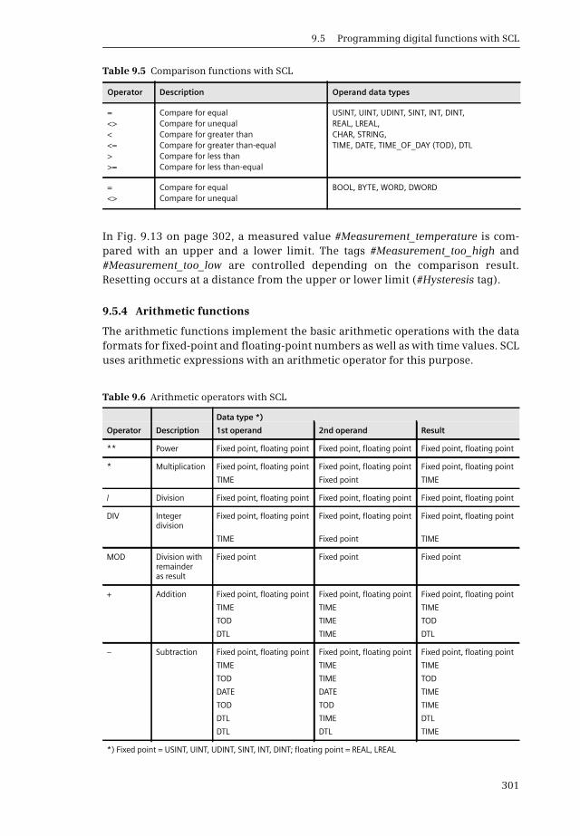
9.5 Programming digital functions with SCL
301
In Fig. 9.13 on page 302, a measured value #Measurement_temperature is com-pared with an upper and a lower limit. The tags #Measurement_too_high and#Measurement_too_low are controlled depending on the comparison result.Resetting occurs at a distance from the upper or lower limit (#Hysteresis tag).
9.5.4 Arithmetic functions
The arithmetic functions implement the basic arithmetic operations with the dataformats for fixed-point and floating-point numbers as well as with time values. SCLuses arithmetic expressions with an arithmetic operator for this purpose.
Table 9.5 Comparison functions with SCL
Operator Description Operand data types
=<><<=>>=
Compare for equalCompare for unequalCompare for greater thanCompare for greater than-equalCompare for less thanCompare for less than-equal
USINT, UINT, UDINT, SINT, INT, DINT, REAL, LREAL, CHAR, STRING, TIME, DATE, TIME_OF_DAY (TOD), DTL
=<>
Compare for equalCompare for unequal
BOOL, BYTE, WORD, DWORD
Table 9.6 Arithmetic operators with SCL
Data type *)
Operator Description 1st operand 2nd operand Result
** Power Fixed point, floating point Fixed point, floating point Fixed point, floating point
* Multiplication Fixed point, floating point Fixed point, floating point Fixed point, floating point
TIME Fixed point TIME
/ Division Fixed point, floating point Fixed point, floating point Fixed point, floating point
DIV Integer division
Fixed point, floating point Fixed point, floating point Fixed point, floating point
TIME Fixed point TIME
MOD Division with remainder as result
Fixed point Fixed point Fixed point
+ Addition Fixed point, floating point Fixed point, floating point Fixed point, floating point
TIME TIME TIME
TOD TIME TOD
DTL TIME DTL
– Subtraction Fixed point, floating point Fixed point, floating point Fixed point, floating point
TIME TIME TIME
TOD TIME TOD
DATE DATE TIME
TOD TOD TIME
DTL TIME DTL
DTL DTL TIME
*) Fixed point = USINT, UINT, UDINT, SINT, INT, DINT; floating point = REAL, LREAL

9 Structured Control Language SCL
302
You can find a detailed description of these arithmetic functions in Chapters 11.3“Arithmetic functions for numerical values” on page 366 and 11.4 “Arithmetic func-tions for time values” on page 369. Table 9.6 shows the arithmetic operators avail-able with SCL with the allowed data types.
The tags or expressions linked to an arithmetic function can have fixed-point, float-ing-point or time value data types. If different data types can be matched in the con-text of implicit data type conversion (see Chapter 4.3.2 “Implicit data type conver-sion” on page 93), a programmed function for (explicit) data type conversion can bedispensed with. The result of an arithmetic function has the “most powerful” of theinvolved data types. If, for example, you link an INT or DINT tag with a REAL tag, theresult is of data type REAL.
In the case of a division, the second operand must not be zero.
In Fig. 9.13, the upper limit of a measured value is monitored under the header“Comparison expressions”. A hysteresis is introduced to ensure that the #Measure-ment_too_high and #Measurement_too_low messages do not “pulsate” when themeasurement changes rapidly around the upper or lower limit. The messages areonly canceled when the measured value has dropped again below the upper limitor risen again above the upper limit by the magnitude of the hysteresis.
There are several calculation examples under the heading “Arithmetic expres-sions”: the calculation of reactive electric power, the volume calculation of a ball,one of the solutions of a quadratic equation, and the formation of an arithmeticmean value.
Fig. 9.13 Examples of comparison expressions, arithmetic and logical expressions
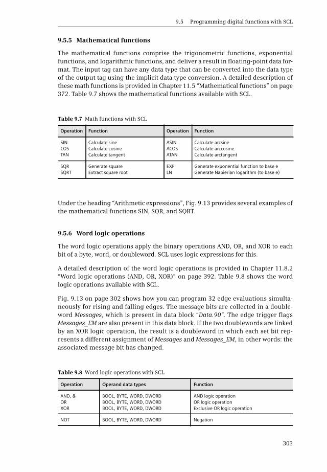
9.5 Programming digital functions with SCL
303
9.5.5 Mathematical functions
The mathematical functions comprise the trigonometric functions, exponentialfunctions, and logarithmic functions, and deliver a result in floating-point data for-mat. The input tag can have any data type that can be converted into the data typeof the output tag using the implicit data type conversion. A detailed description ofthese math functions is provided in Chapter 11.5 “Mathematical functions” on page372. Table 9.7 shows the mathematical functions available with SCL.
Under the heading “Arithmetic expressions”, Fig. 9.13 provides several examples ofthe mathematical functions SIN, SQR, and SQRT.
9.5.6 Word logic operations
The word logic operations apply the binary operations AND, OR, and XOR to eachbit of a byte, word, or doubleword. SCL uses logic expressions for this.
A detailed description of the word logic operations is provided in Chapter 11.8.2“Word logic operations (AND, OR, XOR)” on page 392. Table 9.8 shows the wordlogic operations available with SCL.
Fig. 9.13 on page 302 shows how you can program 32 edge evaluations simulta-neously for rising and falling edges. The message bits are collected in a double-word Messages, which is present in data block “Data.90”. The edge trigger flagsMessages_EM are also present in this data block. If the two doublewords are linkedby an XOR logic operation, the result is a doubleword in which each set bit rep-resents a different assignment of Messages and Messages_EM, in other words: theassociated message bit has changed.
Table 9.7 Math functions with SCL
Operation Function Operation Function
SINCOSTAN
Calculate sineCalculate cosineCalculate tangent
ASINACOSATAN
Calculate arcsineCalculate arccosineCalculate arctangent
SQRSQRT
Generate squareExtract square root
EXPLN
Generate exponential function to base eGenerate Napierian logarithm (to base e)
Table 9.8 Word logic operations with SCL
Operation Operand data types Function
AND, &ORXOR
BOOL, BYTE, WORD, DWORDBOOL, BYTE, WORD, DWORDBOOL, BYTE, WORD, DWORD
AND logic operationOR logic operationExclusive OR logic operation
NOT BOOL, BYTE, WORD, DWORD Negation
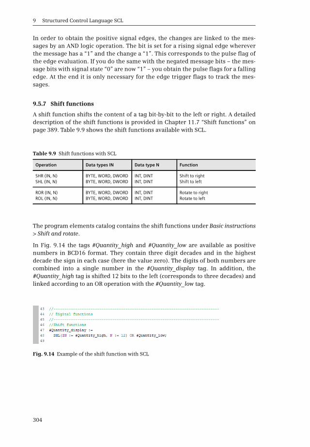
9 Structured Control Language SCL
304
In order to obtain the positive signal edges, the changes are linked to the mes-sages by an AND logic operation. The bit is set for a rising signal edge whereverthe message has a “1” and the change a “1”. This corresponds to the pulse flag ofthe edge evaluation. If you do the same with the negated message bits – the mes-sage bits with signal state “0” are now “1” – you obtain the pulse flags for a fallingedge. At the end it is only necessary for the edge trigger flags to track the mes-sages.
9.5.7 Shift functions
A shift function shifts the content of a tag bit-by-bit to the left or right. A detaileddescription of the shift functions is provided in Chapter 11.7 “Shift functions” onpage 389. Table 9.9 shows the shift functions available with SCL.
The program elements catalog contains the shift functions under Basic instructions> Shift and rotate.
In Fig. 9.14 the tags #Quantity_high and #Quantity_low are available as positivenumbers in BCD16 format. They contain three digit decades and in the highestdecade the sign in each case (here the value zero). The digits of both numbers arecombined into a single number in the #Quantity_display tag. In addition, the#Quantity_high tag is shifted 12 bits to the left (corresponds to three decades) andlinked according to an OR operation with the #Quantity_low tag.
Table 9.9 Shift functions with SCL
Operation Data types IN Data type N Function
SHR (IN, N)SHL (IN, N)
BYTE, WORD, DWORDBYTE, WORD, DWORD
INT, DINTINT, DINT
Shift to rightShift to left
ROR (IN, N)ROL (IN, N)
BYTE, WORD, DWORDBYTE, WORD, DWORD
INT, DINTINT, DINT
Rotate to rightRotate to left
Fig. 9.14 Example of the shift function with SCL
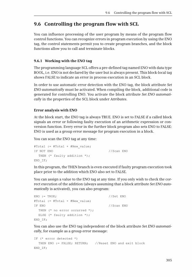
9.6 Controlling the program flow with SCL
305
9.6 Controlling the program flow with SCL
You can influence processing of the user program by means of the program flowcontrol functions. You can recognize errors in program execution by using the ENOtag, the control statements permit you to create program branches, and the blockfunctions allow you to call and terminate blocks.
9.6.1 Working with the ENO tag
The programming language SCL offers a pre-defined tag named ENO with data typeBOOL, i.e. ENO is not declared by the user but is always present. This block-local tagshows FALSE to indicate an error in process execution in an SCL block.
In order to use automatic error detection with the ENO tag, the block attribute SetENO automatically must be activated. When compiling the block, additional code isgenerated for controlling ENO. You activate the block attribute Set ENO automati-cally in the properties of the SCL block under Attributes.
Error analysis with ENO
At the block start, the ENO tag is always TRUE. ENO is set to FALSE if a called blocksignals an error or following faulty execution of an arithmetic expression or con-version function. Every error in the further block program also sets ENO to FALSE:ENO is used as a group error message for program execution in a block.
You can scan the ENO tag at any time:
#Total := #Total + #New_value;
IF NOT ENO //Scan ENO
THEN (* faulty addition *);
END_IF;
In this program, the THEN branch is even executed if faulty program execution tookplace prior to the addition which ENO also set to FALSE.
You can assign a value to the ENO tag at any time. If you only wish to check the cor-rect execution of the addition (always assuming that a block attribute Set ENO auto-matically is activated), you can also program:
ENO := TRUE; //Set ENO
#Total := #Total + #New_value;
IF ENO //Scan ENO
THEN (* no error occurred *);
ELSE (* faulty addition *);
END_IF;
You can also use the ENO tag independent of the block attribute Set ENO automati-cally, for example as a group error message:
IF (* error detected *)
THEN ENO := FALSE; RETURN; //Reset ENO and exit block
END_IF;

9 Structured Control Language SCL
306
When exiting the block, the value of the ENO tag is automatically assigned to theenable output ENO of the block.
Error evaluation following a block call
A block call can control the ENO tag via the enable output ENO. If the enable outputis FALSE (this is the case if an error has occurred in the called block or if the ENO taghas been set to FALSE in the called block by the user), the “block-local” ENO tag isalso set to FALSE in the current block.
"Block" (In1 := ..., In2 := ...);
IF NOT ENO THEN (* an error has occurred up to here *);
END_IF;
An error signaled by the called block – as well as previous errors – sets the “block-local” ENO tag to FALSE. If you wish to scan an error signal by the called block inde-pendent of a previous error, use the enable output ENO:
"Block" (In1 := ..., In2 := ..., ENO => #OK);
IF NOT #OK THEN (* error in block *); END_IF;
The “block-local” ENO tag is not set to FALSE if the called block has not been pro-cessed via the enable input EN (with EN equal to FALSE).
9.6.2 EN/ENO mechanism with SCL
The EN/ENO mechanism is based on the enable input EN and enable output ENO. ENand ENO are implicitly defined parameters with a block call. EN is permissible forfunction blocks (FB), ENO for all block types (even system blocks) which can becalled. EN and ENO are not displayed by the program editor in the offered template.
EN is the first parameter in the parameter list, ENO the last. Use of these parametersis optional. If you do not require these parameters, simply omit them.
The EN/ENO mechanism is only supported in SCL if the block attribute Set ENO auto-matically is activated.
Enable input EN
You can control the calling of a block using the enable input EN. If EN is TRUE or notused, the called block is processed. If EN is FALSE, the called block is not processed.You use the enable input EN in the parameter list like an input parameter:
"Block"(EN := #Enable, In1 := ..., In2 := ...);
(* "Block" is only processed if #Enable = TRUE *)
You can use the enable input to implement a conditional block call, which depends onthe value of a binary tag or binary expression.
Enable output ENO
You can scan the error status of the block using the enable output ENO. If ENO isTRUE, processing has been carried out correctly. If FALSE, the ENO output signals

9.6 Controlling the program flow with SCL
307
that an error is present in the block. You can scan the state of the ENO output in theparameter list using a tag:
"Block" (In1 := ..., In2 := ..., ENO => #OK);
(* With error-free processing, #OK has the value TRUE *)
If the called block signals an error, this is transferred to the block-local ENO tag:
"Block" (In1 := ..., In2 := ..., ENO => #OK);
#No_error := ENO;
IF NOT #OK THEN (* error in block *); END_IF;
IF NOT #No error THEN (* group error message *); END_IF;
The #OK tag is FALSE if block processing was faulty. The #No_error tag is FALSE ifblock processing was faulty or if an error was already present prior to the block call.
If a function block with EN = FALSE is not processed, this has no influence on the“block-local” ENO tag. However, the ENO output is set to FALSE.
"Block"(EN := #Enable, ... , ENO => #OK);
#No_error := ENO;
If the #Enable tag is FALSE, the #OK tag is FALSE and the #No_error tag remainsuninfluenced at its “old” value.
If you wish to use the EN/ENO mechanism to switch more block calls “in series”, youcan program it as follows:
"Block1"(EN := #Enable, ... , ENO => #OK);
"Block2"(EN := #OK, ... );
“Block2” is not processed if #Enable is FALSE or if an error has occurred in “Block1”.
Fig. 9.15 provides a summary of how the enable output ENO and the ENO tag arecontrolled with a block call.
9.6.3 Control statements
The control statements control program branches and loops depending on a condi-tion. The following control statements are used with SCL:
b IF Program branch depending on BOOL value
b CASE Program branch depending on INT value
b FOR Program loop with a loop-control tag
b WHILE Program loop with a feasibility condition
b REPEAT Program loop with an abort condition
b CONTINUE Abort current loop
b EXIT Leave the program loop
Note: Make sure when using program loops that the cycle monitoring time is notexceeded.
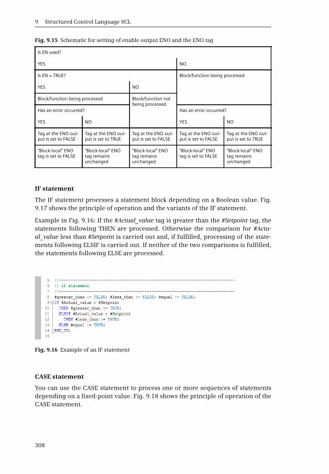
9 Structured Control Language SCL
308
IF statement
The IF statement processes a statement block depending on a Boolean value. Fig.9.17 shows the principle of operation and the variants of the IF statement.
Example in Fig. 9.16: If the #Actual_value tag is greater than the #Setpoint tag, thestatements following THEN are processed. Otherwise the comparison for #Actu-al_value less than #Setpoint is carried out and, if fulfilled, processing of the state-ments following ELSIF is carried out. If neither of the two comparisons is fulfilled,the statements following ELSE are processed.
CASE statement
You can use the CASE statement to process one or more sequences of statementsdepending on a fixed-point value. Fig. 9.18 shows the principle of operation of theCASE statement.
Fig. 9.15 Schematic for setting of enable output ENO and the ENO tag
Is EN used?
YES NO
Is EN = TRUE? Block/function being processed
YES NO
Block/function being processed Block/function not being processed
Has an error occurred? Has an error occurred?
YES NO YES NO
Tag at the ENO out-put is set to FALSE
Tag at the ENO out-put is set to TRUE
Tag at the ENO out-put is set to FALSE
Tag at the ENO out-put is set to FALSE
Tag at the ENO out-put is set to TRUE
“Block-local” ENO tag is set to FALSE
“Block-local” ENO tag remains unchanged
“Block-local” ENO tag remains unchanged
“Block-local” ENO tag is set to FALSE
“Block-local” ENO tag remains unchanged
Fig. 9.16 Example of an IF statement
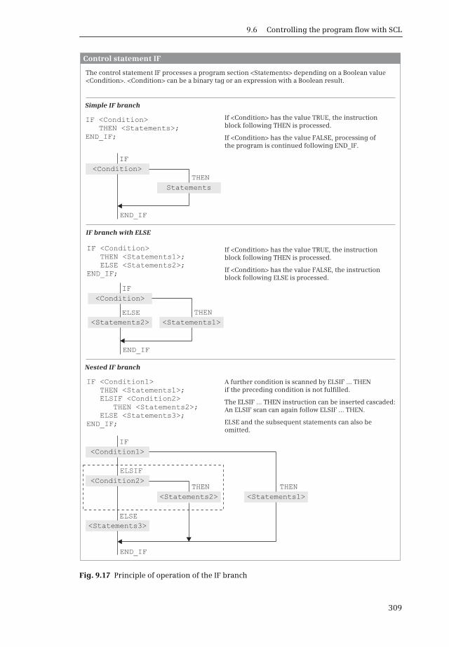
9.6 Controlling the program flow with SCL
309
Fig. 9.17 Principle of operation of the IF branch
Simple IF branch
Nested IF branch
Control statement IF
IF <Condition>THEN <Statements>;
END_IF;
IF <Condition>THEN <Statements1>;ELSE <Statements2>;
END_IF;
IF <Condition1>THEN <Statements1>;ELSIF <Condition2>
THEN <Statements2>;ELSE <Statements3>;
END_IF;
IF
IF
IF
ELSIF
END_IF
END_IF
END_IF
Statements
<Statements1>
<Statements1><Statements2>
<Statements2>
<Statements3>
<Condition>
<Condition>
<Condition1>
<Condition2>
THEN
THEN
THENTHEN
ELSE
ELSE
The control statement IF processes a program section <Statements> depending on a Boolean value <Condition>. <Condition> can be a binary tag or an expression with a Boolean result.
If <Condition> has the value TRUE, the instruction block following THEN is processed.
If <Condition> has the value FALSE, processing of the program is continued following END_IF.
IF branch with ELSE
If <Condition> has the value TRUE, the instruction block following THEN is processed.
If <Condition> has the value FALSE, the instruction block following ELSE is processed.
A further condition is scanned by ELSIF … THEN if the preceding condition is not fulfilled.
The ELSIF … THEN instruction can be inserted cascaded: An ELSIF scan can again follow ELSIF … THEN.
ELSE and the subsequent statements can also be omitted.
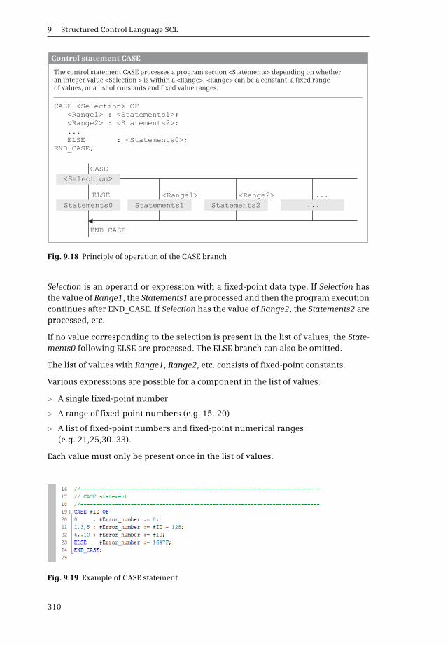
9 Structured Control Language SCL
310
Selection is an operand or expression with a fixed-point data type. If Selection hasthe value of Range1, the Statements1 are processed and then the program executioncontinues after END_CASE. If Selection has the value of Range2, the Statements2 areprocessed, etc.
If no value corresponding to the selection is present in the list of values, the State-ments0 following ELSE are processed. The ELSE branch can also be omitted.
The list of values with Range1, Range2, etc. consists of fixed-point constants.
Various expressions are possible for a component in the list of values:
b A single fixed-point number
b A range of fixed-point numbers (e.g. 15..20)
b A list of fixed-point numbers and fixed-point numerical ranges (e.g. 21,25,30..33).
Each value must only be present once in the list of values.
Fig. 9.18 Principle of operation of the CASE branch
Fig. 9.19 Example of CASE statement
Control statement CASE
CASE <Selection> OF
...ELSE : <Statements0>;
END_CASE;
<Range2> : <Statements2>;
CASE
END_CASE
Statements1Statements0 Statements2 ...
<Selection>
<Range1>ELSE <Range2> ...
The control statement CASE processes a program section <Statements> depending on whether an integer value <Selection > is within a <Range>. <Range> can be a constant, a fixed range of values, or a list of constants and fixed value ranges.
<Range1> : <Statements1>;
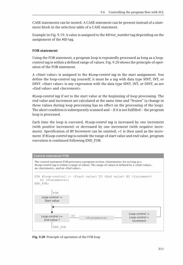
9.6 Controlling the program flow with SCL
311
CASE statements can be nested. A CASE statement can be present instead of a state-ment block in the selection table of a CASE statement.
Example in Fig. 9.19: A value is assigned to the #Error_number tag depending on theassignment of the #ID tag.
FOR statement
Using the FOR statement, a program loop is repeatedly processed as long as a loop-control tag is within a defined range of values. Fig. 9.20 shows the principle of oper-ation of the FOR statement.
A <Start value> is assigned to the #Loop-control tag in the start assignment. Youdefine the loop-control tag yourself; it must be a tag with data type SINT, INT, orDINT. <Start value> is any expression with the data type SINT, INT, or DINT, as are<End value> and <Increment>.
#Loop-control tag if set to the start value at the beginning of loop processing. Theend value and increment are calculated at the same time and “frozen” (a change inthese values during loop processing has no effect on the processing of the loop).The abort condition is subsequently scanned and – if it is not fulfilled – the programloop is processed.
Each time the loop is executed, #Loop-control tag is increased by one increment(with positive increment) or decreased by one increment (with negative incre-ment). Specification of BY Increment can be omitted; +1 is then used as the incre-ment. If #Loop-control tag is outside the range of start value and end value, programexecution is continued following END_FOR.
Fig. 9.20 Principle of operation of the FOR loop
Control statement FOR
DO <Statements>;END_FOR;
FOR
END_FOR
<Statements>
Loop-control :=Start value
Loop-control <=End value ?
Loop-control :=Loop-control +
Increment
DO
The control statement FOR processes a program section <Statements> for as long as a #Loop-control tag is within a range of values. The range of values is defined by a <Start value>,an <Increment>, and an <End value>.
FOR #Loop-control := <Start value> TO <End value> BY <Increment>

9 Structured Control Language SCL
312
The last execution of the loop is carried out with the end value or with the value<End value> minus <Increment> if the end value is not reached exactly. Followinga completely executed program loop, the loop-control tag has the value of the lastloop plus <Increment>.
FOR loops can be nested: Further FOR loops with other loop-control tags can be pro-grammed within the FOR loop. The current program execution can be aborted inthe FOR loop using CONTINUE; EXIT terminates the complete FOR loop processing.
Example in Fig. 9.21: In a #Current data field with 16 components, the maximumvalue is searched for. In the FOR loop, the index tag #Index runs through the values1 to 16. On each cycle, a field component #Current[#Index] is compared with thealready saved value #MaxValue. If #MaxValue is smaller, the value of the component#Current[#Index] is imported.
WHILE statement
The WHILE statement is used to repeatedly process a program loop for as long as afeasibility condition is fulfilled. Fig. 9.22 shows the principle of operation of theWHILE statement.
<Condition> is an operand or expression with data type BOOL. The statements fol-lowing DO are repeatedly processed for as long as <Condition> is TRUE.
Fig. 9.21 Example of the FOR statement
Fig. 9.22 Principle of operation of the WHILE loop
Control statement WHILE
WHILE <Condition>DO <Statements>;
END_WHILE;
WHILE
DO
END_WHILE
StatementsCondition ?
The control statement WHILE processes a program section <Statements> for as long as a <Condition> is fulfilled. <Condition> is a binary tag or an expression with binary result.
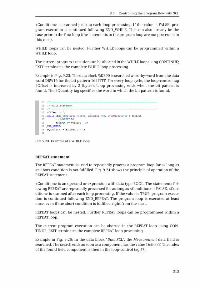
9.6 Controlling the program flow with SCL
313
<Condition> is scanned prior to each loop processing. If the value is FALSE, pro-gram execution is continued following END_WHILE. This can also already be thecase prior to the first loop (the statements in the program loop are not processed inthis case).
WHILE loops can be nested: Further WHILE loops can be programmed within aWHILE loop.
The current program execution can be aborted in the WHILE loop using CONTINUE;EXIT terminates the complete WHILE loop processing.
Example in Fig. 9.23: The data block %DB90 is searched word-by-word from the dataword DBW16 for the bit pattern 16#FFFF. For every loop cycle, the loop-control tag#Offset is increased by 2 (bytes). Loop processing ends when the bit pattern isfound. The #Quantity tag specifies the word in which the bit pattern is found.
REPEAT statement
The REPEAT statement is used to repeatedly process a program loop for as long asan abort condition is not fulfilled. Fig. 9.24 shows the principle of operation of theREPEAT statement.
<Condition> is an operand or expression with data type BOOL. The statements fol-lowing REPEAT are repeatedly processed for as long as <Condition> is FALSE. <Con-dition> is scanned after each loop processing. If the value is TRUE, program execu-tion is continued following END_REPEAT. The program loop is executed at leastonce, even if the abort condition is fulfilled right from the start.
REPEAT loops can be nested: Further REPEAT loops can be programmed within aREPEAT loop.
The current program execution can be aborted in the REPEAT loop using CON-TINUE; EXIT terminates the complete REPEAT loop processing.
Example in Fig. 9.25: In the data block “Data.SCL”, the Measurement data field issearched. The search ends as soon as a component has the value 16#FFFF. The indexof the found field component is then in the loop-control tag #k.
Fig. 9.23 Example of a WHILE loop
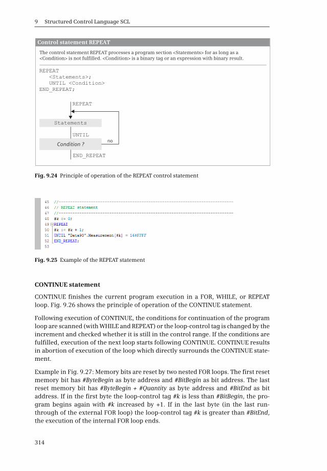
9 Structured Control Language SCL
314
CONTINUE statement
CONTINUE finishes the current program execution in a FOR, WHILE, or REPEATloop. Fig. 9.26 shows the principle of operation of the CONTINUE statement.
Following execution of CONTINUE, the conditions for continuation of the programloop are scanned (with WHILE and REPEAT) or the loop-control tag is changed by theincrement and checked whether it is still in the control range. If the conditions arefulfilled, execution of the next loop starts following CONTINUE. CONTINUE resultsin abortion of execution of the loop which directly surrounds the CONTINUE state-ment.
Example in Fig. 9.27: Memory bits are reset by two nested FOR loops. The first resetmemory bit has #ByteBegin as byte address and #BitBegin as bit address. The lastreset memory bit has #ByteBegin + #Quantity as byte address and #BitEnd as bitaddress. If in the first byte the loop-control tag #k is less than #BitBegin, the pro-gram begins again with #k increased by +1. If in the last byte (in the last run-through of the external FOR loop) the loop-control tag #k is greater than #BitEnd,the execution of the internal FOR loop ends.
Fig. 9.24 Principle of operation of the REPEAT control statement
Fig. 9.25 Example of the REPEAT statement
Control statement REPEAT
REPEAT<Statements>;UNTIL <Condition>
END_REPEAT;
REPEAT
no
END_REPEAT
UNTIL
Statements
Condition ?
The control statement REPEAT processes a program section <Statements> for as long as a<Condition> is not fulfilled. <Condition> is a binary tag or an expression with binary result.
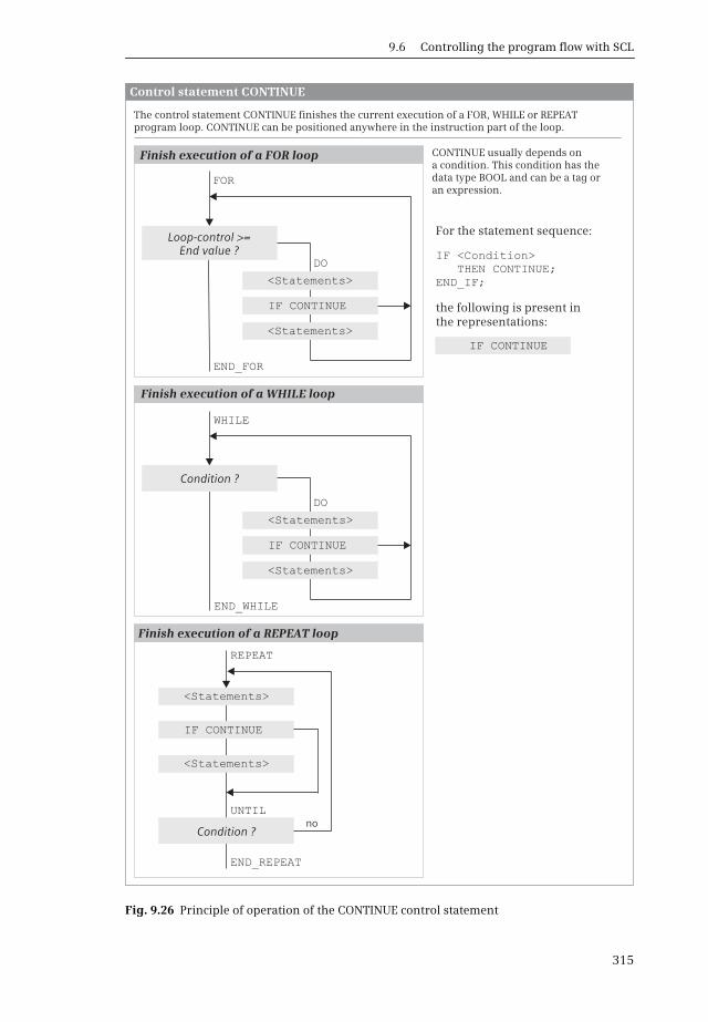
9.6 Controlling the program flow with SCL
315
Fig. 9.26 Principle of operation of the CONTINUE control statement
Control statement CONTINUE
IF <Condition>THEN CONTINUE;
END_IF;
REPEAT
no
END_REPEAT
UNTIL
<Statements>
IF CONTINUE
IF CONTINUE
IF CONTINUE
IF CONTINUE
<Statements>
Condition ?
Finish execution of a REPEAT loop
Finish execution of a FOR loop
Finish execution of a WHILE loop
WHILE
END_WHILE
FOR
END_FOR
<Statements>
<Statements>
<Statements>
<Statements>
Loop-control >=End value ?
Condition ?
DO
DO
For the statement sequence:
the following is present in the representations:
The control statement CONTINUE finishes the current execution of a FOR, WHILE or REPEAT program loop. CONTINUE can be positioned anywhere in the instruction part of the loop.
CONTINUE usually depends on a condition. This condition has the data type BOOL and can be a tag or an expression.

9 Structured Control Language SCL
316
EXIT statement
EXIT leaves a FOR, WHILE, or REPEAT loop at any position independent of condi-tions. Loop processing is aborted immediately and the program following END_-FOR, END_WHILE, or END_REPEAT is processed. Fig. 9.28 shows the principle ofoperation of the EXIT statement.
EXIT results in leaving of the loop which directly surrounds the EXIT statement. Anexample is shown in Fig. 9.27.
9.6.4 Block functions
The block functions call and terminate blocks. A detailed description of the blockfunctions is provided in Chapter 12.3 “Calling of code blocks” on page 413. Fig. 9.29shows examples of the block functions with SCL.
When calling, an SFC system function is treated like an FC function and an SFB sys-tem block is treated like an FB function block. The ENO enable output can be addedas the last parameter to the block parameter list. The application of the enableinput EN is only allowed with function blocks (FB).
Terminate block with RETURN
The RETURN statement terminates processing in the current block. The programelements catalog contains RETURN under Basic instructions > Program control oper-ations.
Example in Fig. 9.29: The block is left if the ENO tag signals an error (is then FALSE).
Call FC block without function value
When calling an FC function, the name of the function is followed by the parameterlist in parentheses. All parameters must be supplied. In Fig. 9.29, the “Adder” func-tion call is used as an example.
Fig. 9.27 Example of the CONTINUE and the EXIT statement
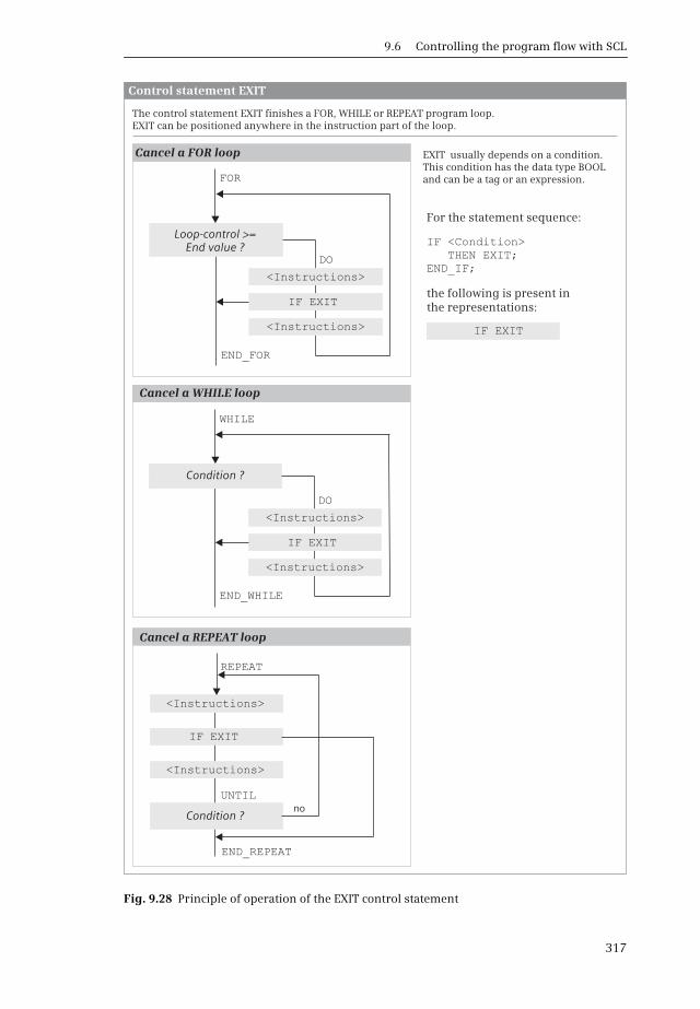
9.6 Controlling the program flow with SCL
317
Fig. 9.28 Principle of operation of the EXIT control statement
Control statement EXIT
REPEAT
no
END_REPEAT
UNTIL
IF EXIT
IF EXIT
IF EXIT
Cancel a REPEAT loop
Cancel a FOR loop
Cancel a WHILE loop
WHILE
END_WHILE
FOR
END_FOR
Condition ?
Condition ?
DO
DO
IF <Condition>THEN EXIT;
END_IF;
IF EXIT
For the statement sequence:
the following is present in the representations:
The control statement EXIT finishes a FOR, WHILE or REPEAT program loop.EXIT can be positioned anywhere in the instruction part of the loop.
<Instructions>
<Instructions>
Loop-control >=End value ?
<Instructions>
<Instructions>
<Instructions>
<Instructions>
EXIT usually depends on a condition. This condition has the data type BOOL and can be a tag or an expression.
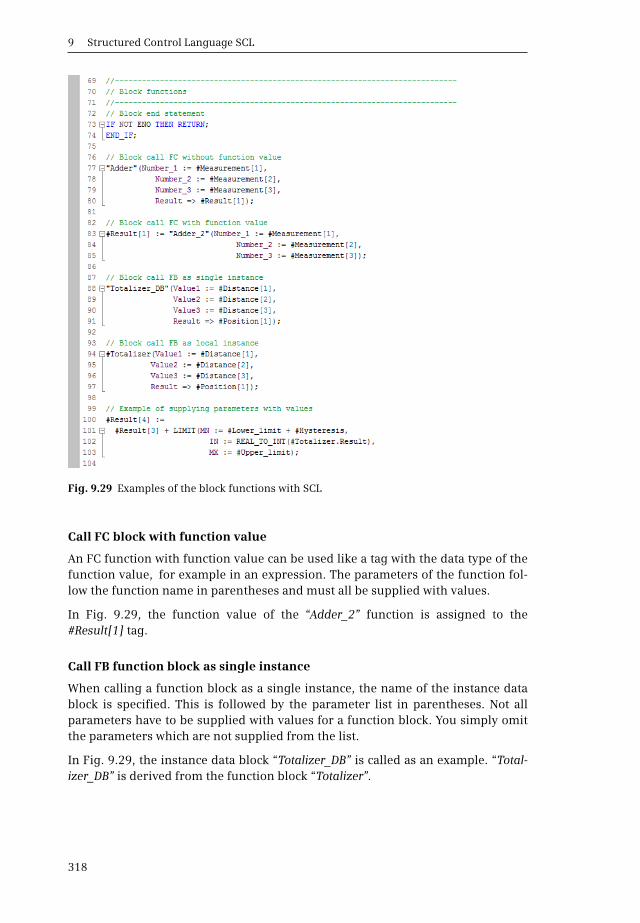
9 Structured Control Language SCL
318
Call FC block with function value
An FC function with function value can be used like a tag with the data type of thefunction value, for example in an expression. The parameters of the function fol-low the function name in parentheses and must all be supplied with values.
In Fig. 9.29, the function value of the “Adder_2” function is assigned to the#Result[1] tag.
Call FB function block as single instance
When calling a function block as a single instance, the name of the instance datablock is specified. This is followed by the parameter list in parentheses. Not allparameters have to be supplied with values for a function block. You simply omitthe parameters which are not supplied from the list.
In Fig. 9.29, the instance data block “Totalizer_DB” is called as an example. “Total-izer_DB” is derived from the function block “Totalizer”.
Fig. 9.29 Examples of the block functions with SCL
9.7 Working with source files
319
Call FB function block as local instance
When calling a function block as local instance, the instance name is followed by theparameter list in parentheses. Not all parameters have to be supplied with valuesfor a function block. You simply omit the parameters which are not supplied fromthe list.
In Fig. 9.29, the local instance #Totalizer is called as an example. #Totalizer isderived from the function block “Totalizer” and is in the instance data block of thecalling function block.
Supplying the block parameters
The input parameters on blocks and functions can be constants, tags, and expres-sions.
In the last example in Fig. 9.29, the #Result[4] tag is assigned a total made up of the#Result[3] tag and the function value (return value) of the standard functionLIMIT. In this case a function with a function value is used within an arithmeticexpression.
The value to be limited by LIMIT is the output parameter of the local instance#Totalizer from the example above this one. It is addressed by #Totalizer.Result andhas the data type REAL. A conversion from REAL to INT must therefore still takeplace at the IN parameter which expects the data type INT. The total of #Lower_limitand #Hysteresis is output as the minimum at the MN parameter.
Additional information about supplying blocks and functions based on blocks withparameters can be found in Chapter 5.4 “Calling blocks” on page 137.
9.7 Working with source files
Blocks with the programming language SCL can be programmed as a text file out-side the TIA Portal. Any text editor which generates ASCII-coded text can be used forthis. Blocks which can be edited further with STEP 7 are generated from these textfiles – referred to as “source files” or “program sources” – by importing into the TIAPortal and subsequent compilation. Blocks programmed with SCL in the TIA Portalcan also be saved as text files.
9.7.1 General procedure
A source file can be generated in two different ways: You write the source file com-pletely using a text editor, or you take a block as template and generate a sourcefile by exporting the block. Following editing with the text editor, you import theexternal source file into the TIA Portal and generate the blocks contained in thesource file by compiling. You can then edit these further using the program editorof STEP 7.

9 Structured Control Language SCL
320
Generating a source file by exporting
In the project tree, select the block(s) from which you wish to generate a source filein the Program blocks folder and select the Copy as text command from the shortcutmenu. The program editor writes the source text into the Windows clipboard.
Open the text editor of your choice – such as the Notepad program in Windows –and paste the content of the clipboard into it. Save the SCL source file with theextension .scl. Files with this extension can be imported as external source filesinto the TIA Portal.
Generating a source file with a text editor
In order to program a block, you must use keywords in a specific sequence in thesource file. The program of each block consists of the block header with specifica-tion of the block type and properties. With logic blocks, this is followed by the dec-laration of the interface and the actual program. With data blocks and PLC datatypes you specify the data operands or data types after the block header.
If the source file contains blocks which are called in the source file or if data oper-ands are accessed, you should observe a specific sequence in the source file. Theblocks or data operands should be located before the position of use in the sourcefile. You can also call blocks in the source file which are present in the Programblocks folder or use system blocks and functions from the program elements cata-log.
A source file can contain several blocks and these can be logic or data blocks as wellas PLC data types. You export and import PLC tags separate from the source file (seeChapter 6.2.4 “Exporting and importing a PLC tag table” on page 181). The follow-ing chapters describe how to program blocks in a source file.
Importing an external source file
To import an external source file, open the External source files folder in the projecttree and double-click on Add new external file. In the dialog box, navigate to thestorage location, select the source file and import it by clicking the Open button.
The source file is saved in the External source files folder.
Editing an external source file in the TIA Portal
As preparation for editing an external source file in the TIA Portal, you must linkthe file extension .scl to a text editor. To do this, open the Windows Explorer, navi-gate to the source file, and select the Properties dialog from the shortcut menu ofthe source file. In the General tab, click on Change in the File type area. Under Openwith, select the editor which you wish to link to the file extension .scl.
You can then edit the source file using the linked editor by double-clicking on it inthe External source files folder.
9.7 Working with source files
321
Generating the blocks of an external source file
To transfer the blocks from the source file to the Program blocks folder, select asource file in the External source files folder and then the Generate blocks commandfrom the shortcut menu. Acknowledge the message which may appear informingthat existing blocks will be overwritten. The generated blocks are imported intothe Program blocks folder. The result of the generation is shown by STEP 7 in theinspector window in the Info > Compile tab. Note that these messages refer to thesource file.
It is recommendable to compile the blocks imported from the source file prior tofurther processing in the TIA Portal.
9.7.2 Programming a logic block in the source file
Table 9.10 shows which keywords you require for block programming and thesequence in which the keywords are used.
Block header and block properties
Programming a logic block commences with the keyword for the block type andwith the specification of the block name in quotation marks. On import, the blockis assigned the first free number of the block type. This can be changed in theblock properties after import.
An organization block has the name of the event class (e.g. “Cyclic interrupt”, seeTable 5.5 on page 154). On import, the organization block is then assigned the firstfree number of the event class (e.g. 30 for event class “Cyclic interrupt”). Only oneorganization block can be imported to a source file per event class.
In the case of functions, you specify the data type of the function value followingthe addressing; example: FUNCTION “FC_name” : INT. If the function does not havea function value, the data type is called VOID.
The block title and the block commentary are entered in the block properties underGeneral > Information.
The data for the block properties is optional. You simply omit the surplus datatogether with the keywords.
You activate the block attribute Optimized block access by specifying {S7_Opti-mized_Access := ’TRUE’}.
The keyword KNOW_HOW_PROTECT protects the block from unwanted access. Youcan no longer cancel this protection, in contrast to block protection with passwordin the TIA Portal.
Block interface
The block interface contains the definition of the block parameters and block-localtags. You cannot program every declaration section in every block (see Table 9.10).If you do not use a declaration section, omit it including the keywords.
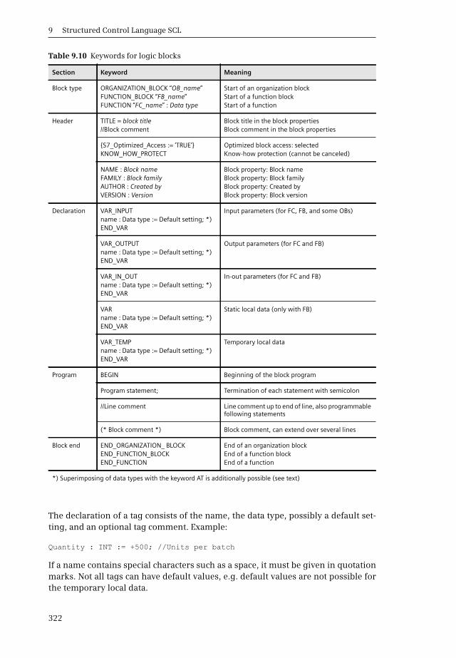
9 Structured Control Language SCL
322
The declaration of a tag consists of the name, the data type, possibly a default set-ting, and an optional tag comment. Example:
Quantity : INT := +500; //Units per batch
If a name contains special characters such as a space, it must be given in quotationmarks. Not all tags can have default values, e.g. default values are not possible forthe temporary local data.
Table 9.10 Keywords for logic blocks
Section Keyword Meaning
Block type ORGANIZATION_BLOCK “OB_name”FUNCTION_BLOCK “FB_name”FUNCTION “FC_name” : Data type
Start of an organization blockStart of a function blockStart of a function
Header TITLE = block title//Block comment
Block title in the block propertiesBlock comment in the block properties
{S7_Optimized_Access := ’TRUE’}KNOW_HOW_PROTECT
Optimized block access: selectedKnow-how protection (cannot be canceled)
NAME : Block nameFAMILY : Block familyAUTHOR : Created byVERSION : Version
Block property: Block nameBlock property: Block familyBlock property: Created byBlock property: Block version
Declaration VAR_INPUTname : Data type := Default setting; *)END_VAR
Input parameters (for FC, FB, and some OBs)
VAR_OUTPUTname : Data type := Default setting; *)END_VAR
Output parameters (for FC and FB)
VAR_IN_OUTname : Data type := Default setting; *)END_VAR
In-out parameters (for FC and FB)
VARname : Data type := Default setting; *)END_VAR
Static local data (only with FB)
VAR_TEMPname : Data type := Default setting; *)END_VAR
Temporary local data
Program BEGIN Beginning of the block program
Program statement; Termination of each statement with semicolon
//Line comment Line comment up to end of line, also programmable following statements
(* Block comment *) Block comment, can extend over several lines
Block end END_ORGANIZATION_ BLOCKEND_FUNCTION_BLOCKEND_FUNCTION
End of an organization blockEnd of a function blockEnd of a function
*) Superimposing of data types with the keyword AT is additionally possible (see text)

9.7 Working with source files
323
The sequence of individual declaration sections is defined as shown in Table 9.10.The sequence within a declaration section is optional. If you combine tags with datatype BOOL and also combine byte-wide tags with data types BYTE and CHAR, youcan minimize the memory requirements for blocks with non-optimized blockaccess.
The superimposition of data types with the keyword AT is programmed directlyafter the declaration of the tags to be overlaid. The schema is as follows: var_newAT var_old : new_data type. Example:
VAR_INPUT Date : DTL; Byte array AT date : ARRAY [1..12] OF BYTE;END_VAR
You can now address the total tag in the program of the block using #Date or indi-vidual components such as the day using #Byte array[3]. Data type superimpositionis possible for blocks with non-optimized block access and is described in Chapter4.3.3 “Overlaying tags (data type views)” on page 93.
Program section
The program section of a logic block starts with the keyword BEGIN and ends withthe keyword for the block end.
No distinction is made between upper and lower case when compiling. The syntaxof an SCL statement is described in Chapter 9.1.2 “SCL statements and operators”on page 286. You can enter one or more spaces or tabulators between operation andoperand. To achieve a clearer layout of the source text, for example to increase leg-ibility, you can enter any spaces and/or tabs between the words.
You must conclude every statement by a semicolon. You can also program severalstatements per line, each separated by a semicolon. Following the semicolon youcan specify a statement comment, separated by two slashes; this extends up to theend of the line.
A line comment commences with two slashes at the start of the line. It extends upto the end of the line. A block comment is started by a round left parenthesis andasterisk and finished by an asterisk and round right parenthesis. A block commentcan extend over several lines.
If the source file contains blocks which are called in the source file or if data oper-ands are accessed, you should observe a specific sequence in the source file. Theblocks or data operands should be located before the position of use in the sourcefile.
When calling a block, you enter the block parameters in round parentheses, eachseparated by a comma. Make sure that the transferred block parameters are listedin the same order as they have been declared in the called block. The same appliesto functions with parameter list from the program elements catalog.
Fig. 9.30 shows an example of an SCL source file for a function block with the asso-ciated instance data block.

9 Structured Control Language SCL
324
FUNCTION_BLOCK FIFOTITLE=Intermediate memory for 4 values
AUTHOR : BergerFAMILY : Book1200NAME : FIFO_SCLVERSION : 01.00
//Example of a function blockVAR_INPUT Import : BOOL := FALSE; //Import with positive edge Input value : REAL := 0.0; //Input in data format REALEND_VAR
VAR_OUTPUT Output value : REAL := 0.0; //Output in data format REALEND_VAR
VAR Value1 : REAL := 0.0; //First saved REAL value Value2 : REAL := 0.0; //Second value Value3 : REAL := 0.0; //Third value Value4 : REAL := 0.0; //Fourth value Edge trigger flag : BOOL := FALSE;//Edge trigger flag for importingEND_VAR
BEGIN//Control is implemented with positive edge on #Import// IF #Import = TRUE AND #Edge trigger flag = FALSE THEN#Output value := #Value4;#Value4 := #Value3; //Transfer starting with the last value#Value3 := #Value2;#Value2 := #Value1;#Value1 := #Input value;END_IF;
#Edge trigger flag := #Import; //Update edge trigger flag
END_FUNCTION_BLOCK
DATA_BLOCK DB_FIFOTITLE = Instance data block for "FIFO"//Example of an instance data block
AUTHOR : BergerFAMILY : Book1200NAME : FIFO_DatVERSION : 01.00
"FIFO" //Instance for the FB "FIFO"
BEGIN Value1 := 1.0; //Individual default setting Value2 := 1.0; //of selected valuesEND_DATA_BLOCK
Fig. 9.30 Example of an SCL source file

9.7 Working with source files
325
9.7.3 Programming a data block in the source file
Table 9.11 shows which keywords you require for block programming and thesequence in which the keywords are used.
Block header and block properties
A data block commences with the keyword DATA_BLOCK and with specification ofthe block name in quotation marks. On import, the first free data block number isassigned. It can be changed later in the block properties.
The block title and the block commentary are entered in the block properties underGeneral > Information.
The data for the block properties is optional. You simply omit the surplus datatogether with the keywords.
You activate the block attribute Optimized block access by specifying {S7_Opti-mized_Access := ’TRUE’}.
The keyword KNOW_HOW_PROTECT protects the block from unwanted access. Youcan no longer cancel this protection, in contrast to block protection with passwordin the TIA Portal.
Table 9.11 Keywords for data blocks
Section Keyword Meaning
Block type DATA_BLOCK “DB_name” Start of a data block
Header TITLE = block title//Block comment
Block titleBlock comment
{S7_Optimized_Access := ’TRUE’}KNOW_HOW_PROTECTUNLINKEDREAD_ONLY
Optimized block access: selectedKnow-how protection (cannot be canceled)Block attribute: not executableBlock attribute: read-only
NAME : Block nameFAMILY : Block familyAUTHOR : Created byVERSION : Version
Block property: Block nameBlock property: Block familyBlock property: Created byBlock property: Block version
Declaration STRUCTname : Data type := Default setting;END_STRUCT
for a global data block
Data type_name alternatively for a type data block
FB_name alternatively for an instance data block
Initialization BEGINname := Default setting; Assignment with individual initial values
Block end END_DATA_BLOCK End of a data block

9 Structured Control Language SCL
326
With the keyword UNLINKED, the Only store in load memory attribute is activated.In this way, the data block is not loaded to the work memory.
The keyword READ_ONLY activates the Data block write-protected in device attribute.If this attribute is activated for a data block, a program can only read from this datablock.
Block interface
The block interface contains the declaration of the data operands. With a globaldata block, you program the data operand here, with a type data block, you specifythe assigned PLC data type, and with an instance data block, you assign the associ-ated function block.
The declaration of a tag in a global data block consists of the name, the data type,possibly a default setting, and an optional tag comment. Example:
Quantity : INT := +500; //Units per batch
The tag order can be random. If you combine tags with data type BOOL and alsocombine byte-wide tags with data types BYTE and CHAR, you can minimize thememory requirements for a block with non-optimized block access.
The declaration in a type data block consists only of the specification of theassigned PLC or system data type, e.g. IEC_COUNTER. Data blocks derived from asystem data type are stored in the project tree under Program blocks > System blocks> Program resources.
The declaration in an instance data block consists only of the specification of theassigned function block.
Default setting with start values
The initialization part starts with BEGIN and ends with END_DATA_BLOCK. Youmust specify these keywords even if you do not assign default values to the tags inthe initialization part.
By assigning default values to the start values, it is possible to assign individual val-ues to each application (each instance) in the case of type and instance data blocks.
If you do not specify a start value for a data operand, the value from the block inter-face is used: The default value is retained for a global data block and the defaultvalue in the PLC data type or in the function block then applies to a type or instancedata block.
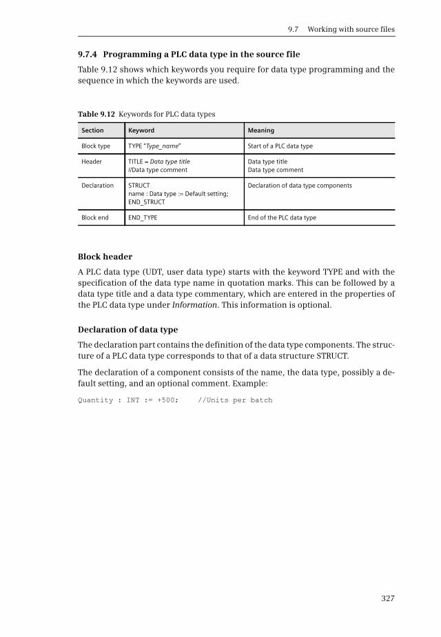
9.7 Working with source files
327
9.7.4 Programming a PLC data type in the source file
Table 9.12 shows which keywords you require for data type programming and thesequence in which the keywords are used.
Block header
A PLC data type (UDT, user data type) starts with the keyword TYPE and with thespecification of the data type name in quotation marks. This can be followed by adata type title and a data type commentary, which are entered in the properties ofthe PLC data type under Information. This information is optional.
Declaration of data type
The declaration part contains the definition of the data type components. The struc-ture of a PLC data type corresponds to that of a data structure STRUCT.
The declaration of a component consists of the name, the data type, possibly a de-fault setting, and an optional comment. Example:
Quantity : INT := +500; //Units per batch
Table 9.12 Keywords for PLC data types
Section Keyword Meaning
Block type TYPE “Type_name” Start of a PLC data type
Header TITLE = Data type title//Data type comment
Data type titleData type comment
Declaration STRUCTname : Data type := Default setting;END_STRUCT
Declaration of data type components
Block end END_TYPE End of the PLC data type
10 Basic functions
328
10 Basic functions
This chapter describes the basic functions largely independent of the programminglanguage selected. Binary logic operations are an exception, since the differencesbetween the programming languages are greatest with these functions. The Chap-ters 7 “Ladder logic LAD” on page 209, 8 “Function block diagram FBD” on page 246,and 9 “Structured Control Language SCL” on page 284 describe how you can pro-gram the functions using the individual programming languages and what specialfeatures exist.
10.1 Binary logic operations
10.1.1 Introduction
Binary logic operations link the signal states of binary tags in accordance with AND,OR, and exclusive OR. In the LAD programming language, they are implemented bythe series and parallel connection of contacts, in FBD by the corresponding functionboxes, and in SCL by logical expressions.
Binary logic operations can be used together with all binary tags. Addressing of thebinary tags can be absolute or symbolic. A binary tag has the data type BOOL andcan have signal state “1” or “0”. In SCL, the designations TRUE and FALSE are com-mon.
The result of a binary logic operation can be processed further as follows:
b Control of a binary tag with a binary memory function, e.g. with a simple coil (LAD) or an assignment (FBD, SCL).
b Control of program execution with a conditional jump or a conditional block call (EN input).
b Supply of a binary function input or a binary block parameter.
Binary logic operations can be combined together so that, for example, the outputof one logic operation can lead to the input of the next one, or series connectionscan be connected in parallel. Possible combinations are described for LAD in Chap-ter 7.2.5 “Mixed series and parallel connections” on page 216, for FBD in Chapter8.2.6 “Mixed binary logic operations” on page 254, and for SCL in Chapter 9.2.6“Combined binary logic operations” on page 292.

10.1 Binary logic operations
329
10.1.2 Scanning for signal states “1” and “0”, result of the scan
Before the signal state of a binary tag is linked, the binary tag is set to either signalstate “1” or scanned for signal state “0” and a scan result is formed. Only the scanresult will be linked. The result of logic operation (RLO) is formed from all linkedscan results. LAD uses the NC contact to scan for signal state “0”, FBD uses the nega-tion circle at the function inputs, and SCL uses the negation NOT (Fig. 10.1).
There are signal transmitters, e.g. pushbuttons, which when actuated issue signalstate “1” (pushbuttons with NO function) or signal state “0” (pushbuttons with NCfunction). The scans for signal states “1” and “0” can be used to take into accountthis difference in creating the program. Further information can be found for LADin Chapter 7.2.2 “Consideration of sensor type in ladder logic” on page 213, forFBD in Chapter 8.2.2 “Taking account of the sensor type in the function block dia-gram” on page 251, and for SCL in Chapter 9.2.1 “Scanning for signal states “1”and “0”” on page 288.
10.1.3 Negating the result of the logic operation, NOT contact
Ladder logic
The NOT contact negates the “current flow” within a current path. If the currentpath has “current” prior to the NOT contact, no more “current” flows following theNOT contact and vice versa (Fig. 10.2).
Fig. 10.1 Scanning for signal state “1” (NO contact) an “0” (NC contact)
LADNO contactNC contact
FBD
SCLScanning for signal states “1” and “0”
Binary tag
Binary tag
... Binary tag ... ... NOT Binary tag ...
Binary tag
Function
Scan signal state
“0”
“0”
“0” “1”
“1”
“1”Binary tag
Tag, function Signal state
Scanning for signal states “1” and “0”
If the binary tag is 1, the NO contact is closed or when scanned for “1”, the scan result is “1”.If the binary tag is “0”, the NC contact is closed or when scanned for “0”, the scan result is “1”.
NO contact, scanning for “1”NC contact, scanning for “0”
Binary tag
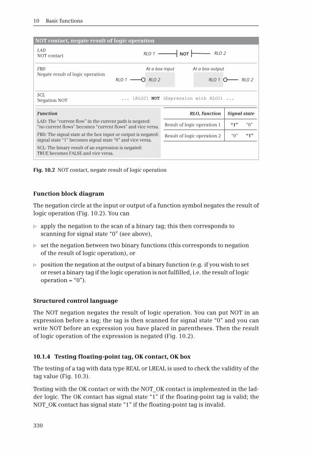
10 Basic functions
330
Function block diagram
The negation circle at the input or output of a function symbol negates the result oflogic operation (Fig. 10.2). You can
b apply the negation to the scan of a binary tag; this then corresponds to scanning for signal state “0” (see above),
b set the negation between two binary functions (this corresponds to negation of the result of logic operation), or
b position the negation at the output of a binary function (e.g. if you wish to set or reset a binary tag if the logic operation is not fulfilled, i.e. the result of logic operation = “0”).
Structured control language
The NOT negation negates the result of logic operation. You can put NOT in anexpression before a tag; the tag is then scanned for signal state “0” and you canwrite NOT before an expression you have placed in parentheses. Then the resultof logic operation of the expression is negated (Fig. 10.2).
10.1.4 Testing floating-point tag, OK contact, OK box
The testing of a tag with data type REAL or LREAL is used to check the validity of thetag value (Fig. 10.3).
Testing with the OK contact or with the NOT_OK contact is implemented in the lad-der logic. The OK contact has signal state “1” if the floating-point tag is valid; theNOT_OK contact has signal state “1” if the floating-point tag is invalid.
Fig. 10.2 NOT contact, negate result of logic operation
LADNOT contact
SCLNegation NOT
FBDNegate result of logic operation
Function
At a box input At a box output
NOTRLO 1
RLO 1RLO 1 RLO 2RLO 2
RLO 2
NOT contact, negate result of logic operation
“0”
“0” “1”
“1”Result of logic operation 1
Result of logic operation 2
RLO, function Signal state
... [ ] (Expression with RLO1) ...RLO2 NOT
LAD: The “current flow” in the current path is negated: “no current flows” becomes “current flows” and vice versa.
FBD: The signal state at the box input or output is negated: signal state “1” becomes signal state “0” and vice versa.
SCL: The binary result of an expression is negated: TRUE becomes FALSE and vice versa.
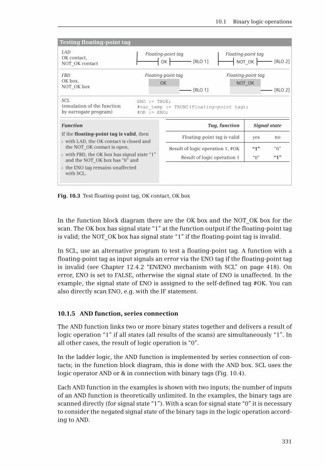
10.1 Binary logic operations
331
In the function block diagram there are the OK box and the NOT_OK box for thescan. The OK box has signal state “1” at the function output if the floating-point tagis valid; the NOT_OK box has signal state “1” if the floating-point tag is invalid.
In SCL, use an alternative program to test a floating-point tag. A function with afloating-point tag as input signals an error via the ENO tag if the floating-point tagis invalid (see Chapter 12.4.2 “EN/ENO mechanism with SCL” on page 418). Onerror, ENO is set to FALSE, otherwise the signal state of ENO is unaffected. In theexample, the signal state of ENO is assigned to the self-defined tag #OK. You canalso directly scan ENO, e.g. with the IF statement.
10.1.5 AND function, series connection
The AND function links two or more binary states together and delivers a result oflogic operation “1” if all states (all results of the scans) are simultaneously “1”. Inall other cases, the result of logic operation is “0”.
In the ladder logic, the AND function is implemented by series connection of con-tacts; in the function block diagram, this is done with the AND box. SCL uses thelogic operator AND or & in connection with binary tags (Fig. 10.4).
Each AND function in the examples is shown with two inputs; the number of inputsof an AND function is theoretically unlimited. In the examples, the binary tags arescanned directly (for signal state “1”). With a scan for signal state “0” it is necessaryto consider the negated signal state of the binary tags in the logic operation accord-ing to AND.
Fig. 10.3 Test floating-point tag, OK contact, OK box
Floating-point tag
Floating-point tag Floating-point tag
Testing floating-point tag
LADOK contact,NOT_OK contact
SCL
FBDOK box,NOT_OK box
Function
OK NOT_OK
OK
[RLO 1]
[RLO 1] [RLO 2]
[RLO 2]
NOT_OK
yes
“0”
“0” “1”
“1”
noFloating-point tag is valid
Tag, function Signal state
n
n
n
ENO := TRUE;#var_temp := TRUNC( );#OK := ENO;
Floating-point tag
Floating-point tag
(emulation of the function by surrogate program)
Result of logic operation 1, #OK
Result of logic operation 1
If the floating-point tag is valid, then
with LAD, the OK contact is closed and the NOT_OK contact is open,
with FBD, the OK box has signal state “1” and the NOT_OK box has “0” and
the ENO tag remains unaffected with SCL.
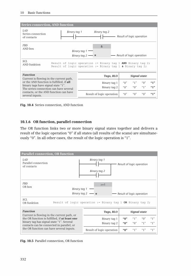
10 Basic functions
332
10.1.6 OR function, parallel connection
The OR function links two or more binary signal states together and delivers aresult of the logic operation “0” if all states (all results of the scans) are simultane-ously “0”. In all other cases, the result of the logic operation is “1”.
Fig. 10.4 Series connection, AND function
Fig. 10.5 Parallel connection, OR function
LADSeries connection of contacts
Binary tag 1 Binary tag 2
“0”
“0”
“0”
“0” “0” “0”
“0”
“1”
“1” “1”
“1”
“1”
Binary tag 1
Result of logic operation
Result of logic operation
Result of logic operation
&FBDAND box
SCLAND funktion
Function Signal state
Series connection, AND function
Result of logic operation := Binary tag 1 AND Binary tag 2;
*Binary tag 2
Current is flowing in the current path, or the AND function is fulfilled, if all binary tags have signal state “1”. The series connection can have several contacts, or the AND function can have several inputs.
Result of logic operation := Binary tag 1 & Binary tag 2;
Tags, RLO
Binary tag 1
Binary tag 2
LAD Parallel connection of contacts
Binary tag 1
Binary tag 2
Binary tag 1
Binary tag 2 Result of logic operation
Result of logic operation
>=1FBDOR box
Function
“0”
“0”
“0”
“0” “1” “1”
“0”
“1”
“1” “1”
“1”
“1”
Result of logic operation
Signal stateTags, RLO
Binary tag 1
Binary tag 2
Parallel connection, OR function
SCLOR funktion
*
Current is flowing in the current path, or the OR function is fulfilled, if at least one binary tag has signal state “1”. Several contacts can be connected in parallel, or the OR function can have several inputs.
Result of logic operation := Binary tag 1 OR Binary tag 2;
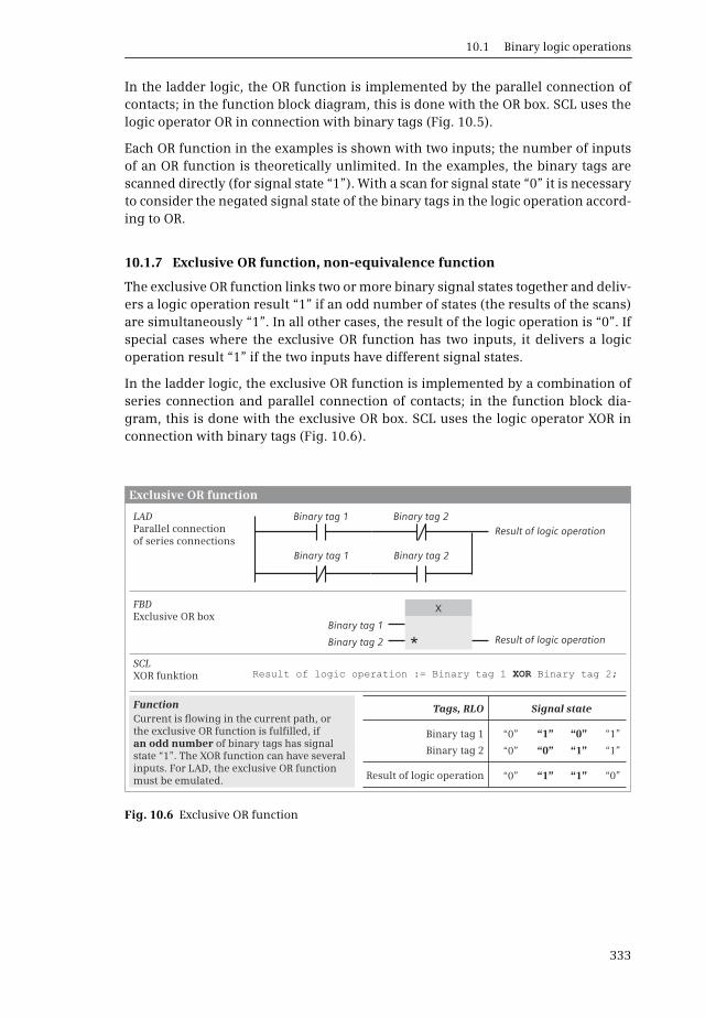
10.1 Binary logic operations
333
In the ladder logic, the OR function is implemented by the parallel connection ofcontacts; in the function block diagram, this is done with the OR box. SCL uses thelogic operator OR in connection with binary tags (Fig. 10.5).
Each OR function in the examples is shown with two inputs; the number of inputsof an OR function is theoretically unlimited. In the examples, the binary tags arescanned directly (for signal state “1”). With a scan for signal state “0” it is necessaryto consider the negated signal state of the binary tags in the logic operation accord-ing to OR.
10.1.7 Exclusive OR function, non-equivalence function
The exclusive OR function links two or more binary signal states together and deliv-ers a logic operation result “1” if an odd number of states (the results of the scans)are simultaneously “1”. In all other cases, the result of the logic operation is “0”. Ifspecial cases where the exclusive OR function has two inputs, it delivers a logicoperation result “1” if the two inputs have different signal states.
In the ladder logic, the exclusive OR function is implemented by a combination ofseries connection and parallel connection of contacts; in the function block dia-gram, this is done with the exclusive OR box. SCL uses the logic operator XOR inconnection with binary tags (Fig. 10.6).
Fig. 10.6 Exclusive OR function
LAD
Result of logic operation
Result of logic operation
XFBDExclusive OR box
Function
Exclusive OR function
*SCLXOR funktion
Binary tag 1
Binary tag 2
Parallel connection of series connections
Binary tag 2Binary tag 1
Binary tag 2Binary tag 1
Current is flowing in the current path, or the exclusive OR function is fulfilled, if an odd number of binary tags has signal state “1”. The XOR function can have several inputs. For LAD, the exclusive OR function must be emulated.
“0”
“0”
“0”
“0” “1” “1”
“0”
“1”
“1” “1”
“0”
“1”
Result of logic operation
Signal stateTags, RLO
Binary tag 1
Binary tag 2
Result of logic operation := Binary tag 1 XOR Binary tag 2;
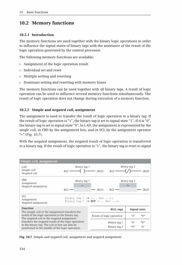
10 Basic functions
334
10.2 Memory functions
10.2.1 Introduction
The memory functions are used together with the binary logic operations in orderto influence the signal states of binary tags with the assistance of the result of thelogic operation generated by the control processor.
The following memory functions are available:
b Assignment of the logic operation result
b Individual set and reset
b Multiple setting and resetting
b Dominant setting and resetting with memory boxes
The memory functions can be used together with all binary tags. A result of logicoperation can be used to influence several memory functions simultaneously. Theresult of logic operation does not change during execution of a memory function.
10.2.2 Simple and negated coil, assignment
The assignment is used to transfer the result of logic operation to a binary tag. Ifthe result of logic operation is “1”, the binary tag is set to signal state “1”; if it is “0”,the binary tag is set to signal state “0”. In LAD, the assignment is represented by thesingle coil, in FBD by the assignment box, and in SCL by the assignment operator“=” (Fig. 10.7).
With the negated assignment, the negated result of logic operation is transferredto a binary tag. If the result of logic operation is “1”, the binary tag is reset to signal
Fig. 10.7 Simple and negated coil, assignment and negated assignment
LADSimple coilNegated coil
RLO
RLO
RLO
RLO (RLO)(RLO)
(RLO)(RLO)
= I=
FBDAssignmentNegated assignment
SCLAssignmentNegated assignment
Function
“0”
“0”
“0” “1”
“1”
“1”
Signal state
Simple coil, assignment
The simple coil or the assignment transfers the result of the logic operation to the binary tag. The negated coil or the negated assignment transfers the negated result of the logic operation to the binary tag. The coil or box can also be positioned in the middle of the logic operation.
Binary tag 1Binary tag 1
(... ...);:= RLO(... ...);:= NOT RLO
Binary tag 1
Binary tag 1 Binary tag 2
Binary tag 2
Binary tag 1
RLO, tags
Binary tag 2
Result of logic operation

10.2 Memory functions
335
state “0”; if it is “0”, the binary tag is set to signal state “1”. The negated assignmentis represented in LAD by the negated coil, and in FBD by the negated assignmentbox. SCL uses the negation NOT to negate a result of logic operation.
In LAD and FBD, the assignment does not influence the result of logic operation sothat a logic operation can also be continued after the assignment function.
10.2.3 Single set and reset
Single setting sets a binary tag to signal state “1” if the result of logic operation is“1”. The binary tag is not influenced if the result of logic operation is “0”; it remainsset if it was set, and remains reset if it was reset. The individual setting is repre-sented in LAD by the set coil, and in FBD by the set box. In SCL, the set function canbe emulated with an IF statement (Fig. 10.8).
Single resetting sets a binary tag to signal state “0” if the result of logic operationis “1”. The binary tag is not influenced if the result of logic operation is “0”; itremains set if it was set, and remains reset if it was reset. The individual resettingis represented in LAD by the reset coil, and in FBD by the reset box. In SCL, the resetfunction can be emulated with an IF statement.
Individual setting and resetting does not affect the result of logic operation in LADand FBD so that a logic operation can be continued even after the set and reset func-tion.
To make the programming clearer, you should always use the single set and resetfunction in pairs for a specific binary tag, and only once each. You should also avoidcontrolling this binary tag in addition by an assignment.
Fig. 10.8 Single setting and resetting
“0”
“0” “1”
“1”
S R
Function
LADS coil,R coil
FBDS box,R box
SCL
Signal state
Single setting and resetting
If the result of the logic operation is “1”, the tag for the S coil or S box is set, and the tag for the R coil or R box is reset. A logic operation result “0” has no effect. The coil or box can also be positioned in the middle of the logic operation.
RLO
RLO
RLO
RLO (RLO)(RLO)
(RLO)(RLO)
S R
IF [RLO] THENBinary tag 1 Binary tag 2:= TRUE;
END_IF;
IF [RLO] THEN:= FALSE;
END_IF;
Binary tag 1
Binary tag 1 Binary tag 2
Binary tag 2
Binary tag 1
RLO, tags
Binary tag 2
Result of logic operation
Unchanged
Unchanged
Nachbildung mitder IF-Anweisung
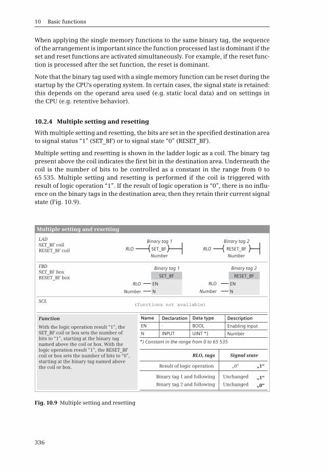
10 Basic functions
336
When applying the single memory functions to the same binary tag, the sequenceof the arrangement is important since the function processed last is dominant if theset and reset functions are activated simultaneously. For example, if the reset func-tion is processed after the set function, the reset is dominant.
Note that the binary tag used with a single memory function can be reset during thestartup by the CPU's operating system. In certain cases, the signal state is retained:this depends on the operand area used (e.g. static local data) and on settings inthe CPU (e.g. retentive behavior).
10.2.4 Multiple setting and resetting
With multiple setting and resetting, the bits are set in the specified destination areato signal status “1” (SET_BF) or to signal state “0” (RESET_BF).
Multiple setting and resetting is shown in the ladder logic as a coil. The binary tagpresent above the coil indicates the first bit in the destination area. Underneath thecoil is the number of bits to be controlled as a constant in the range from 0 to65 535. Multiple setting and resetting is performed if the coil is triggered withresult of logic operation “1”. If the result of logic operation is “0”, there is no influ-ence on the binary tags in the destination area; then they retain their current signalstate (Fig. 10.9).
Fig. 10.9 Multiple setting and resetting
LADSET_BF coilRESET_BF coil
Number Number
Number Number
SET_BF RESET_BFRLO
RLO RLO
RLO
Multiple setting and resetting
With the logic operation result “1”, the SET_BF coil or box sets the number of bits to “1”, starting at the binary tag named above the coil or box. With the logic operation result “1”, the RESET_BF coil or box sets the number of bits to “0”, starting at the binary tag named above the coil or box.
FBDSET_BF boxRESET_BF box
SCL
Function
SET_BF
EN
N N
DeclarationName
EN
N
-
INPUT
*) Constant in the range from 0 to 65 535
BOOL
UINT *)
Enabling input
Number
DescriptionData type
Result of logic operation
„0“
„0“ „1“
„1“
Signal state
RESET_BF
EN
Binary tag 1 Binary tag 2
Binary tag 1 Binary tag 2
(functions not available)
RLO, tags
Binary tag 1 and following
Binary tag 2 and following
Unchanged
Unchanged
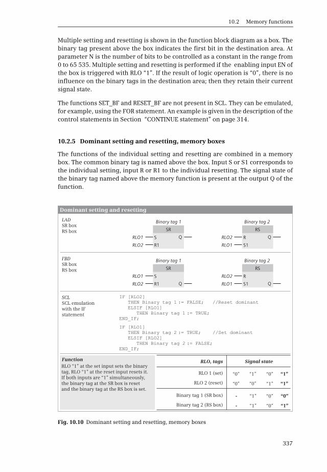
10.2 Memory functions
337
Multiple setting and resetting is shown in the function block diagram as a box. Thebinary tag present above the box indicates the first bit in the destination area. Atparameter N is the number of bits to be controlled as a constant in the range from0 to 65 535. Multiple setting and resetting is performed if the enabling input EN ofthe box is triggered with RLO “1”. If the result of logic operation is “0”, there is noinfluence on the binary tags in the destination area; then they retain their currentsignal state.
The functions SET_BF and RESET_BF are not present in SCL. They can be emulated,for example, using the FOR statement. An example is given in the description of thecontrol statements in Section “CONTINUE statement” on page 314.
10.2.5 Dominant setting and resetting, memory boxes
The functions of the individual setting and resetting are combined in a memorybox. The common binary tag is named above the box. Input S or S1 corresponds tothe individual setting, input R or R1 to the individual resetting. The signal state ofthe binary tag named above the memory function is present at the output Q of thefunction.
Fig. 10.10 Dominant setting and resetting, memory boxes
LADSR boxRS box
FBDSR boxRS box
SCLSCL emulation with the IF statement
Function
Binary tag 1 (SR box)
RLO, tags
Binary tag 2 (RS box)
RLO 1 (set)
RLO 2 (reset)
RLO1
RLO1
RLO2
RLO2
RLO2
RLO2
RLO1
RLO1
Signal state
SR
SR
RS
RS
S
S
R
R
R1
R1
S1
S1
Q
Q
Q
Q
Dominant setting and resetting
IF [RLO2]THEN Binary tag 1 := FALSE; //Reset dominantELSIF [RLO1]
THEN Binary tag 1 := TRUE;END_IF;
IF [RLO1]THEN Binary tag 2 := TRUE; //Set dominantELSIF [RLO2]
THEN Binary tag 2 := FALSE;END_IF;
RLO “1” at the set input sets the binary tag, RLO “1” at the reset input resets it. If both inputs are “1” simultaneously, the binary tag at the SR box is reset and the binary tag at the RS box is set.
Binary tag 1
Binary tag 1
Binary tag 2
Binary tag 2
- “0”
“1” “1”
“0” “0”
“0” “1”
“1” “1”
“0” “1”
- “0”
“1” “0”
10 Basic functions
338
There are two versions of the memory function: as SR box (reset dominant) and asRS box (set dominant). In addition to the difference in labeling, the two boxes alsodiffer in the positioning of the set and reset inputs (Fig. 10.10).
A memory function (or, to be more precise: the binary tag named above the memo-ry box), is set when the set input has signal state “1” and the reset input signalstate “0”. A memory function is reset when “1” is present at the reset input and “0”at the set input. Signal state “0” at both inputs has no influence on a memory func-tion. If signal state “1” is present simultaneously at both inputs, the two memoryfunctions respond differently: the SR memory function is reset, the RS memoryfunction is set.
With SCL, the dominant memory function can be emulated, for example, by anassignment together with an IF statement.
Note that the binary tag used with a memory function can be reset during the start-up by the CPU's operating system. In certain cases, the signal state of a memory boxis retained: this depends on the operand area used (e.g. static local data) and on set-tings in the CPU (e.g. retentive behavior).
10.3 Edge evaluation
10.3.1 Functional principle of an edge evaluation
An edge evaluation records the change in a signal state, i.e. the signal edge.A positive (rising) edge is present if the signal changes from state “0” to state “1”.The reverse case is a negative (falling) edge.
The equivalent of an edge evaluation in a circuit diagram is a fleeting contact. If thefleeting contact outputs a pulse when the relay is switched on, this corresponds tothe rising edge. A pulse of the fleeting contact when switching off corresponds to afalling edge.
The detection of a signal edge – the change in a signal state – is implemented in theprogram. When processing an edge evaluation, the CPU compares the currentresult of logic operation, e.g. the result of scan of an input, with a saved result oflogic operation. If the two signal states are different, a signal edge is present.
The saved result of the logic operation (RLO) is in a so-called “edge memory bit”(it need not necessarily be a bit memory). It must be a binary tag whose signal stateis available again during the next processing of the edge evaluation (in the nextprogram cycle) and which you do not use at any further point in the program. Suit-able binary tags are memory bits, data bits in global data blocks, and static local da-ta bits in function blocks.
These edge memory bits save the “old” RLO, namely the result of the logic operationwith which the CPU last processed the edge evaluation. If a signal edge is then pres-ent, i.e. if the current RLO is different from the signal state of the edge memory bit,the CPU tracks the signal state of the edge memory bit by assigning it to the RLO
10.3 Edge evaluation
339
which is now current. During the next processing of the edge evaluation (usually inthe next program cycle), the signal state of the edge memory bit is equal to the cur-rent RLO (if this has not changed again in the meantime), and the CPU no longerrecognizes an edge.
A recognized edge is indicated by the RLO following the edge evaluation. If the CPUrecognizes a signal edge, it sets the RLO following the edge evaluation to “1” (“cur-rent” is then flowing). If a signal edge is not present, the RLO is equal to “0”.
Signal state “1” following an edge evaluation therefore means “ Edge detected”. Sig-nal state “1” is only present briefly, usually for only one processing cycle. Since theCPU does not detect an edge during the next processing of the edge evaluation(if the “Input RLO” of the edge evaluation does not change), it sets the RLO to “0”again following the edge evaluation.
You can directly process the RLO following an edge evaluation, e.g. link using bina-ry logic operations, save in a memory function, or assign to a binary tag (a so-called“pulse flag”). A pulse flag is used if the RLO of the edge evaluation is to be also pro-cessed at another position in the program; it is quasi the intermediate memory fora detected edge (the fleeting contact in the circuit diagram). Suitable binary tags forthe pulse flag are memory bits, data bits in global data blocks, and temporary andstatic local data bits.
Also take note of the response of edge evaluation when switching on the CPU. If anedge should not be detected, the RLO prior to edge evaluation and the signal stateof the edge trigger flag must be the same when switching on. It may be necessary –depending on the desired response and the operand area used – to appropriatelyset or reset the edge trigger flag during the startup.
Principle of operation of the positive edge (Fig. 10.11): a In the initial state, the sig-nal being monitored for an edge, the edge trigger flag, and the pulse flag have sig-nal state “0”. s The edge signal then changes its state from “0” to “1”. The signalstate of the edge trigger flag is initially still “0” so that a rising edge is detected andthe pulse flag is set to “1”. The edge trigger flag is updated to signal state “1”. d Thenext processing cycle does not show a change in the signal state or edge signal(comparison with signal state of edge trigger flag). The pulse flag is reset to “0”. fNo changes take place in the next processing cycles. g If the edge signal is reset tostate “0” again, the edge trigger flag is also updated and the initial state is reached.The pulse flag was therefore only set to “1” for one processing cycle.
Functional principle of the negative edge: a In the initial state, the edge signal, theedge memory bit, and the pulse flag have the signal state “0”. s The edge thenchanges its signal state from “0” to “1”. This change is saved in the edge memory bitwhich is also set to “1”. The pulse flag remains “0” since a falling edge is not present.d There is no change in the next processing cycles. f The edge signal then changesfrom “1” to “0”. The edge memory bit initially still has signal state “1” so that a fall-ing edge is detected. The pulse flag is set to “1”, and the edge memory bit trackedto “0”. g The pulse flag is reset to “0” again. The pulse flag was therefore only setto “1” for the duration of one processing cycle.
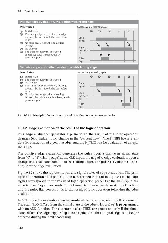
10 Basic functions
340
10.3.2 Edge evaluation of the result of the logic operation
This edge evaluation generates a pulse when the result of the logic operationchanges (with ladder logic: change in the “current flow”). The P_TRIG box is avail-able for evaluation of a positive edge, and the N_TRIG box for evaluation of a nega-tive edge.
The positive edge evaluation generates the pulse upon a change in signal statefrom “0” to “1” (rising edge) at the CLK input, the negative edge evaluation upon achange in signal state from “1” to “0” (falling edge). The pulse is available at the Qoutput of the edge evaluation.
Fig. 10.12 shows the representation and signal states of edge evaluation. The prin-ciple of operation of edge evaluation is described in detail in Fig. 10.11: The edgesignal corresponds to the result of logic operation present at the CLK input, theedge trigger flag corresponds to the binary tag named underneath the function,and the pulse flag corresponds to the result of logic operation following the edgeevaluation.
In SCL, the edge evaluation can be emulated, for example, with the IF statement.The scan “RLO differs from the signal state of the edge trigger flag” is programmedwith an AND function. The statements after THEN are processed only if the signalstates differ. The edge trigger flag is then updated so that a signal edge is no longerdetected during the next processing.
Fig. 10.11 Principle of operation of an edge evaluation in successive cycles
Edge signal
Edge signal
Edge memory bit
Edge memory bit
Pulse flag
Pulse flag
Positive edge evaluation, evaluation with rising edge
Negative edge evaluation, evaluation with falling edge
Description
Description Successive processing cycles
Successive processing cycles
Initial stateThe rising edge is detected, the edge memory bit is tracked, the pulse flag is setNo edge any longer, the pulse flag is resetNo changeThe edge memory bit is tracked, the initial state is subsequently present again
Initial stateThe edge memory bit is trackedNo changeThe falling edge is detected, the edge memory bit is tracked, the pulse flag is setNo edge any longer, the pulse flag is reset, the initial state is subsequently present again

10.3 Edge evaluation
341
10.3.3 Edge evaluation of a binary tag
The edge evaluation of a binary tag is represented in the ladder logic as a contact,above which the scanned binary tag and below which the edge trigger flag arenamed. The pulse of the edge evaluation (quasi the signal state of the pulse flag) isconnected in series with the result of logic operation of the preceding logic opera-tion. A positive, rising edge is detected by the P contact and a negative, falling edgeby the N contact.
In the function block diagram, the binary tag is named above the edge evaluationbox, and the edge memory bit below it. The Q output corresponds to the pulse flag.A positive, rising edge is detected by the P box, and a negative, falling edge by theN box.
In SCL, the edge evaluation can be emulated, for example, with the IF statement.The scan “The signal states of the binary tag and edge trigger flag are different” isprogrammed with an AND function. The statements after THEN are processed only
Fig. 10.12 Edge evaluation of result of logic operation (of the “current flow”)
LAD, FBDP_TRIG-Box
LAD, FBDN_TRIG-Box
SCLSCL emulation with the IF statement
Positive (rising) edge
Negative (falling) edge
Edge memory bit 1
Edge memory bit 2
RLO1
RLO3
RLO2
RLO4
P_TRIG
N_TRIG
CLK
CLK
Q
Q
a
a
s
s
d
d
f
f
g
g
RLO1
RLO3
Processing cycles
Processing cycles
Edge memory bit 1
Edge memory bit 2
RLO2
RLO4
Function
Edge evaluation of result of logic operation (of “current flow”)
IF [RLO1] AND NOT Edge trigger flag1THEN
END_IF;Edge trigger flag1 := [RLO1];
IF NOT [RLO3] AND Edge trigger flag2THEN
END_IF;Edge trigger flag2 := [RLO3];
“0”
“0”
“1”
“1”
“1”
“0”
“0”
“0”
“1”
“0”
“0”
“1”
“0”
“0”
“1”
“1”
“1”
“0”
“0”“
“0”
“0”
“0”
“0”
“0”
“0”
“0”
“0”
“0”
“0”
“0”
//positive edge
//update edge trigger flag
//negative edge
//update edge trigger flag
(*...instructions [corresponds to RLO2]...*);
(*...instructions [corresponds to RLO4]...*);
P_TRIG: If a positive signal edge is detected at the CLK input, the Q output has signal state “1” for the duration of one cycle (in processing cycle s in the table).
N_TRIG: If a negative signal edge is detected at the CLK input, the Q output has signal state “1” for the duration of one cycle (in processing cycle d in the table).
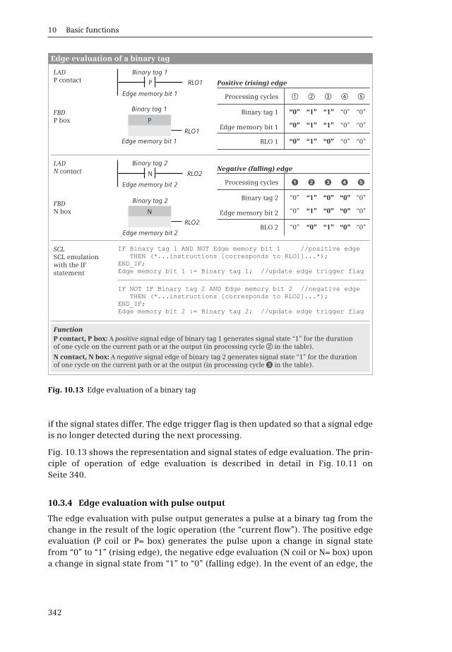
10 Basic functions
342
if the signal states differ. The edge trigger flag is then updated so that a signal edgeis no longer detected during the next processing.
Fig. 10.13 shows the representation and signal states of edge evaluation. The prin-ciple of operation of edge evaluation is described in detail in Fig. 10.11 onSeite 340.
10.3.4 Edge evaluation with pulse output
The edge evaluation with pulse output generates a pulse at a binary tag from thechange in the result of the logic operation (the “current flow”). The positive edgeevaluation (P coil or P= box) generates the pulse upon a change in signal statefrom “0” to “1” (rising edge), the negative edge evaluation (N coil or N= box) upona change in signal state from “1” to “0” (falling edge). In the event of an edge, the
Fig. 10.13 Edge evaluation of a binary tag
P
N
RLO1
RLO2
LADP contact
LADN contact
SCL
P boxFBD
N boxFBD
Positive (rising) edge
Negative (falling) edge
RLO1
RLO2
P
N
Function
Edge evaluation of a binary tag
//positive edge
END_IF;Edge memory bit 1 := Binary tag 1; //update edge trigger flag
//negative edge
END_IF;//update edge trigger flag
Binary tag 1
Edge memory bit 1
Binary tag 1
Edge memory bit 1
Binary tag 2
Edge memory bit 2
Binary tag 2
Edge memory bit 2
SCL emulation with the IF statement
“0”
“1”
“1”
“0” “1” “0”
“0”
“1”
“1” “0” “0”
“0” “0”
“0” “0”Binary tag 1
Processing cycles
Edge memory bit 1
RLO 1
“0”
“1”
“0”
“0” “0” “1”
“0”
“1”
“0” “0” “0”
“0” “0”
“0” “0”Binary tag 2
Processing cycles
Edge memory bit 2
RLO 2
P contact, P box: A positive signal edge of binary tag 1 generates signal state “1” for the duration of one cycle on the current path or at the output (in processing cycle s in the table).
N contact, N box: A negative signal edge of binary tag 2 generates signal state “1” for the duration of one cycle on the current path or at the output (in processing cycle d in the table).
IF Binary tag 1 AND NOT Edge memory bit 1THEN (*...instructions [corresponds to RLO1]...*);
IF NOT IF Binary tag 2 AND Edge memory bit 2THEN (*...instructions [corresponds to RLO2]...*);
Edge memory bit 2 := Binary tag 2;

10.3 Edge evaluation
343
binary tag has signal state “1” for the duration of one processing cycle. The resultof the logic operation following the contact or at the output of the box corre-sponds to the result of the logic operation prior to the contact or box – it is simply“passed on”.
In SCL the pulse flag is set to signal state “1” if the result of logic operation and thesignal state of the edge trigger flag are different. The edge trigger flag is thenupdated so that a signal edge is no longer detected during the next processing andthe pulse flag is reset to signal state “0”.
The function of the edge evaluation is shown in Fig. 10.14; the description corre-sponds to that in Fig. 10.12 on Seite 341. Here, the edge signal corresponds to theresult of preceding logic operation (the “current flow”).
Fig. 10.14 Edge evaluation with pulse output
SCL
Function
Edge evaluation with pulse output
//update edge trigger flag
//update edge trigger flag
LADP coil
LADN coil
FBDP=-Box
FBDN=-box
Edge memory bit 1
Edge memory bit 2
RLO1
RLO2
Pulse flag 1
Pulse flag 2
P
N
Positive (rising) edge
Negative (falling) edge
Edge memory bit 1
Edge memory bit 2
Pulse flag 1
Pulse flag 2
RLO1
RLO2
(RLO1)
(RLO2)
(RLO1)
(RLO2)
P=
N=
“0”
“0”
“1”
“1”
“1”
“0”
“0”
“0”
“1”
“0”
“0”
“1”
“0”
“0”
“1”
“1”
“1”
“0”
“0”
“0”
“0”
“0”
“0”
“0”
“0”
“0”
“0”
“0”
“0”
“0”
RLO 1
RLO 2
Processing cycles
Processing cycles
Edge memory bit 1
Edge memory bit 2
Pulse flag 1
Pulse flag 2
Emulation with the IF statement
P coil, P=-box: If a positive signal edge occurs (RLO 1) in front of the P coil or at the input of the P=-box, pulse flag 1 has signal state “1” for the duration of one cycle (in processing cycle in the table). After the P-coil or P=-box, there is the same RLO as before the coil or box (RLO 1).
s
N coil, N=-box: If a negative signal edge occurs (RLO 2) in front of the N coil or at the input of the N=-box, pulse flag 1 has signal state “1” for the duration of one cycle (in processing cycle in the table). After the N-coil or N=-box, there is the same RLO as before the coil or box (RLO 2).
d
//The pulse flag is set with positive edge.
//The pulse flag is set with negative edge.
Pulse flag 1 := [RLO1] AND NOT Edge memory bit 1;Edge memory bit 1 := [RLO1];//During the next cycle the pulse flag will be reset.
//During the next cycle the pulse flag will be reset.
Pulse flag 2 := NOT [RLO2] AND Edge memory bit 2;Edge memory bit 2 := [RLO2];

10 Basic functions
344
10.4 Time functions
10.4.1 Introduction
The timer functions implement timing processes in the user program such as wait-ing and monitoring times, measurement of a time interval, or the generation ofpulses. The following timer functions are available:
b TP Pulse generation
b TON ON delay
b TOF OFF delay
b TONR Accumulating ON delay
Fig. 10.15 shows the statements in connection with the timer functions.
A time function is a statement with its own data. When programming a time func-tion, you specify the data block in which the data is to be saved. If you select theSingle instance button, it must be a different data block each time. If you program atime function in a function block, you can also select Multi-instance. The data of thetime function is then saved as a local instance in the instance data block of the func-tion block.
The data structure of a timer function is mapped in the system data type (SDT)IEC_TIMER. The individual components of the data structure is shown in Section4.8.1 “IEC_TIMER system data type” on page 110.
The data from several timer functions can be stored in an instance data block underdifferent names. This reduces the number of required data blocks. You can also takeadvantage of this when calling timer functions in FC and OB blocks: In a global datablock, you create a tag with the data type IEC_TIMER for each call of a timer functionand cancel the Call options dialog when programming the timer function. Instead,you specify the tag name for the storage location of the instance data. Example: Ifin the data block “Timer data” you create a Pulse tag with data type IEC_TIMER, youcan specify the instance name “Timer_Data”.Pulse when calling the timer function.
When calling a timer function TP, TON, TOF, or TONR, you must supply the startinput IN and the defined duration PT (preset time) with tags. Supplying of the timerstatus Q and the elapsed time value ET is optional. You can scan the time status likea binary tag at any point in the user program with Instance_Name.Q.
LAD and FBD know statements that only start a timer function, reset a timer func-tion (RT, Reset Timer), and set a new duration (PT, Preset Timer).
The time functions run in the STARTUP and RUN modes.
Note that the instance data of a timer function is only updated if you call one of thestatements TP, TON, TOF, and TONR or on direct access to the structure compo-nents Q (time status) and ET (current time value). Thus it may happen that thescans of the time status or the current time value deliver different values at two dif-ferent points in the program. You can avoid different values in a program cycle if
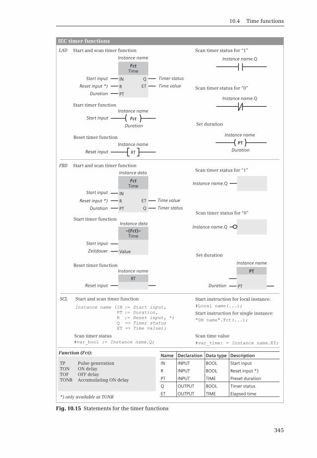
10.4 Time functions
345
Fig. 10.15 Statements for the timer functions
Name Declaration Data type Description
IN INPUT BOOL Start input
R INPUT BOOL Reset input *)
PT INPUT TIME
Q OUTPUT BOOL Timer status
ET OUTPUT TIME Elapsed time
IEC timer functions
Start and scan timer function
Start timer function
Start and scan timer function
Start timer function
Reset timer function
Reset timer function
Start and scan timer function Start instruction for local instance:
Start instruction for single instance:
#Local name(...);
"DB name".Fct(...);
Scan timer status for “1”
Scan timer status for “0”
Set duration
Scan timer status Scan time value
Set duration
SCL
Function (Fct):
Reset input Duration
Instance name
Instance name.Q
Instance name
Instance name.Q
PT
PT
LAD
FBD
IN
IN
R
PT
R
PT
Q
ET
ET
Q
Instance data
FctTime
Instance name
Instance name
Instance name
Duration
Reset input *)
Duration
Reset input *)
Duration
Zeitdauer
Start input
Start input
Start input
Timer status
Time value
Timer status
Time value
Reset input Duration
Fct
PT
Start input
Instance data
–( )–
Value
TP Pulse generationTON ON delayTOF OFF delayTONR Accumulating ON delay
Instance name (INPT
QET
#var_time: = Instance name.ET;
RT
RT
Instance name
Scan timer status for “1”
Scan timer status for “0”
Instance name.Q
Instance name.Q
RTimer statusTime value);
Start input,Duration,Reset input, *)
=>=>
:=:=:=
#var_bool := Instance name.Q;
Preset duration
*) only available at TONR
FctTime
FctTime
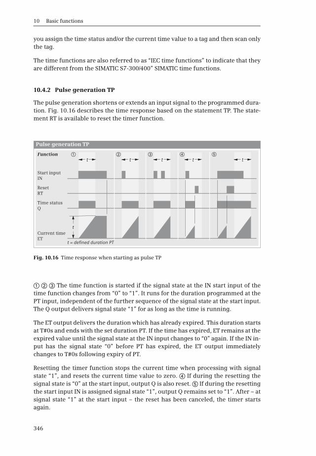
10 Basic functions
346
you assign the time status and/or the current time value to a tag and then scan onlythe tag.
The time functions are also referred to as “IEC time functions” to indicate that theyare different from the SIMATIC S7-300/400” SIMATIC time functions.
10.4.2 Pulse generation TP
The pulse generation shortens or extends an input signal to the programmed dura-tion. Fig. 10.16 describes the time response based on the statement TP. The state-ment RT is available to reset the timer function.
a s d The time function is started if the signal state at the IN start input of thetime function changes from “0” to “1”. It runs for the duration programmed at thePT input, independent of the further sequence of the signal state at the start input.The Q output delivers signal state “1” for as long as the time is running.
The ET output delivers the duration which has already expired. This duration startsat T#0s and ends with the set duration PT. If the time has expired, ET remains at theexpired value until the signal state at the IN input changes to “0” again. If the IN in-put has the signal state “0” before PT has expired, the ET output immediatelychanges to T#0s following expiry of PT.
Resetting the timer function stops the current time when processing with signalstate “1”, and resets the current time value to zero. f If during the resetting thesignal state is “0” at the start input, output Q is also reset. g If during the resettingthe start input IN is assigned signal state “1”, output Q remains set to “1”. After – atsignal state “1” at the start input – the reset has been canceled, the timer startsagain.
Fig. 10.16 Time response when starting as pulse TP
Pulse generation TP
t = defined duration PT
Time statusQ
Current timeET
Start inputIN
t t t tta s d f g
ResetRT
Function
t
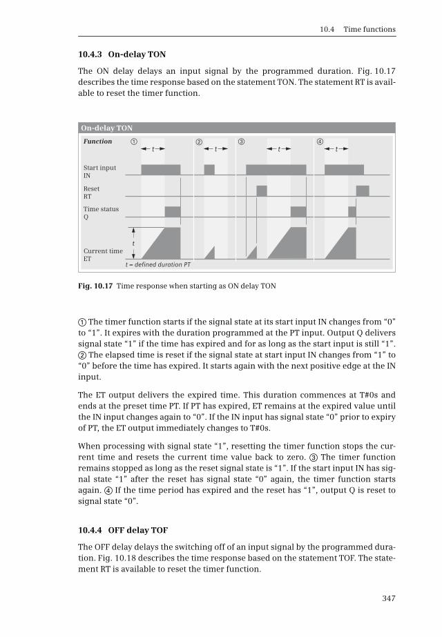
10.4 Time functions
347
10.4.3 On-delay TON
The ON delay delays an input signal by the programmed duration. Fig. 10.17describes the time response based on the statement TON. The statement RT is avail-able to reset the timer function.
a The timer function starts if the signal state at its start input IN changes from “0”to “1”. It expires with the duration programmed at the PT input. Output Q deliverssignal state “1” if the time has expired and for as long as the start input is still “1”.s The elapsed time is reset if the signal state at start input IN changes from “1” to“0” before the time has expired. It starts again with the next positive edge at the INinput.
The ET output delivers the expired time. This duration commences at T#0s andends at the preset time PT. If PT has expired, ET remains at the expired value untilthe IN input changes again to “0”. If the IN input has signal state “0” prior to expiryof PT, the ET output immediately changes to T#0s.
When processing with signal state “1”, resetting the timer function stops the cur-rent time and resets the current time value back to zero. d The timer functionremains stopped as long as the reset signal state is “1”. If the start input IN has sig-nal state “1” after the reset has signal state “0” again, the timer function startsagain. f If the time period has expired and the reset has “1”, output Q is reset tosignal state “0”.
10.4.4 OFF delay TOF
The OFF delay delays the switching off of an input signal by the programmed dura-tion. Fig. 10.18 describes the time response based on the statement TOF. The state-ment RT is available to reset the timer function.
Fig. 10.17 Time response when starting as ON delay TON
On-delay TON
t = defined duration PT
Time statusQ
Start inputIN
t t tta s d f
Current timeET
Function
ResetRT
t
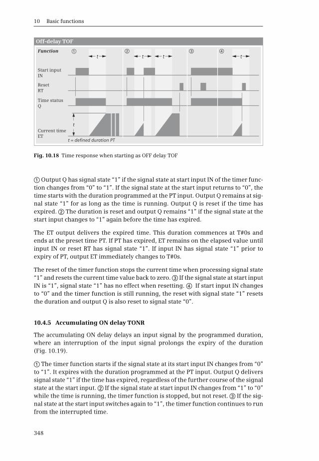
10 Basic functions
348
a Output Q has signal state “1” if the signal state at start input IN of the timer func-tion changes from “0” to “1”. If the signal state at the start input returns to “0”, thetime starts with the duration programmed at the PT input. Output Q remains at sig-nal state “1” for as long as the time is running. Output Q is reset if the time hasexpired. s The duration is reset and output Q remains “1” if the signal state at thestart input changes to “1” again before the time has expired.
The ET output delivers the expired time. This duration commences at T#0s andends at the preset time PT. If PT has expired, ET remains on the elapsed value untilinput IN or reset RT has signal state “1”. If input IN has signal state “1” prior toexpiry of PT, output ET immediately changes to T#0s.
The reset of the timer function stops the current time when processing signal state“1” and resets the current time value back to zero. d If the signal state at start inputIN is “1”, signal state “1” has no effect when resetting. f If start input IN changesto “0” and the timer function is still running, the reset with signal state “1” resetsthe duration and output Q is also reset to signal state “0”.
10.4.5 Accumulating ON delay TONR
The accumulating ON delay delays an input signal by the programmed duration,where an interruption of the input signal prolongs the expiry of the duration(Fig. 10.19).
a The timer function starts if the signal state at its start input IN changes from “0”to “1”. It expires with the duration programmed at the PT input. Output Q deliverssignal state “1” if the time has expired, regardless of the further course of the signalstate at the start input. s If the signal state at start input IN changes from “1” to “0”while the time is running, the timer function is stopped, but not reset. d If the sig-nal state at the start input switches again to “1”, the timer function continues to runfrom the interrupted time.
Fig. 10.18 Time response when starting as OFF delay TOF
Off-delay TOF
Time statusQ
Start inputIN
t tt ta s d f
t = defined duration PT
Current timeET
ResetRT
Function
t
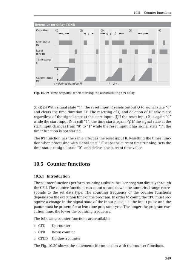
10.5 Counter functions
349
a s d With signal state “1”, the reset input R resets output Q to signal state “0”and clears the time duration ET. The resetting of Q and deletion of ET take placeregardless of the signal state at the start input. fIf the reset input R is again “0”while the start input IN is still “1”, the time starts again. g If the signal state at thestart input changes from “0” to “1” while the reset input R has signal state “1”, thetimer function is not started.
The RT function has the same effect as the reset input R. Resetting the timer func-tion when processing with signal state “1” stops the current time running, sets thetime status to signal state “0”, and deletes the current time value.
10.5 Counter functions
10.5.1 Introduction
The counter functions perform counting tasks in the user program directly throughthe CPU. The counter functions can count up and down; the numerical range corre-sponds to the set data type. The counting frequency of the counter functionsdepends on the execution time of the program. In order to count, the CPU must rec-ognize a change in the signal state of the input pulse, i.e. the input pulse and thepause must be present for at least one program cycle. The longer the program exe-cution time, the lower the counting frequency.
The following counter functions are available:
b CTU Up counter
b CTD Down counter
b CTUD Up-down counter
The Fig. 10.20 shows the statements in connection with the counter functions.
Fig. 10.19 Time response when starting the accumulating ON delay
Retentive on-delay TONR
ResetR or RT
Time statusQ
Start inputIN
Functiont t t2
t1 + t2 = t
t1 ta gs d f
t = defined duration PT
Current timeET
t
+
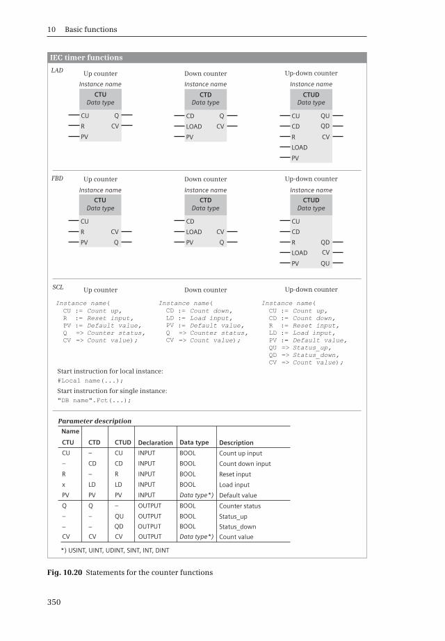
10 Basic functions
350
Fig. 10.20 Statements for the counter functions
IEC timer functions
Up counter Down counter Up-down counter
Up counter Down counter Up-down counter
Up counter Down counter Up-down counter
SCL
LAD
FBD
Instance name(CUCDRLDPVQU
CVQD
Instance name(CDLDPVQCV
Instance name(CURPVQCV
Counter status,Count value);
Count up,Reset input,Default value,
=>=>
:=:=:=
DeclarationCTUDCTDCTU
Name
CU–CU
CDCD–
R–R
LDLDx
PV
–
PVPV
QU
Q
–
–
Q
–
– QD
CVCVCV
INPUT
INPUT
INPUT
INPUT
INPUT
OUTPUT
OUTPUT
OUTPUT
OUTPUT
BOOL
BOOL
BOOL
BOOL
Data type*)
BOOL
BOOL
BOOL
Data type*)
Count up input
Count down input
Reset input
Load input
Default value
Status_up
Counter status
Status_down
Count value
DescriptionData type
CTUD
CTUD
CU
CU
R
R
PV
PV
CD
CD
LOAD
LOAD
QU
QD
CV
QU
QD
CV
*) USINT, UINT, UDINT, SINT, INT, DINT
CTUData type
CTU
CU
CU
R
R
PV
PV
Q
CV
CV
Q
Instance name
Instance name
Instance name
Instance name
Instance name
Instance name
CTD
CTD
CD
CD
LOAD
LOAD
PV
PV
Q
CV
CV
Q
Parameter description
Data type
Data type
Data type
Data type
Data type
Counter status,Count value);
Count down,Load input,Default value,
=>=>
:=:=:=
Start instruction for local instance:
Start instruction for single instance:
#Local name(...);
"DB name".Fct(...);
Count up,Count down,Reset input,
:=:=:=
Status_down,Count value);
Load input,Default value,
=>=>
:=:=
Status_up,=>
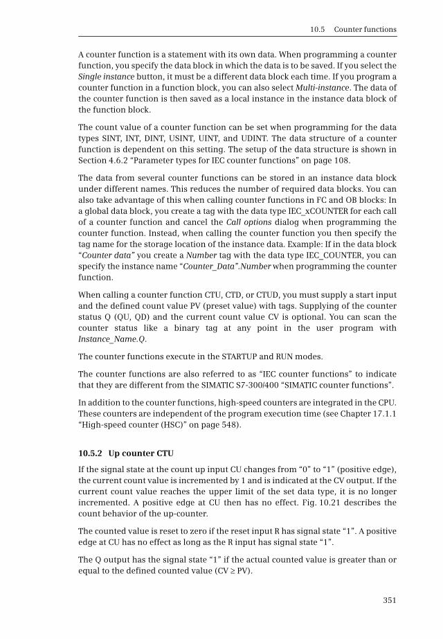
10.5 Counter functions
351
A counter function is a statement with its own data. When programming a counterfunction, you specify the data block in which the data is to be saved. If you select theSingle instance button, it must be a different data block each time. If you program acounter function in a function block, you can also select Multi-instance. The data ofthe counter function is then saved as a local instance in the instance data block ofthe function block.
The count value of a counter function can be set when programming for the datatypes SINT, INT, DINT, USINT, UINT, and UDINT. The data structure of a counterfunction is dependent on this setting. The setup of the data structure is shown inSection 4.6.2 “Parameter types for IEC counter functions” on page 108.
The data from several counter functions can be stored in an instance data blockunder different names. This reduces the number of required data blocks. You canalso take advantage of this when calling counter functions in FC and OB blocks: Ina global data block, you create a tag with the data type IEC_xCOUNTER for each callof a counter function and cancel the Call options dialog when programming thecounter function. Instead, when calling the counter function you then specify thetag name for the storage location of the instance data. Example: If in the data block“Counter data” you create a Number tag with the data type IEC_COUNTER, you canspecify the instance name “Counter_Data”.Number when programming the counterfunction.
When calling a counter function CTU, CTD, or CTUD, you must supply a start inputand the defined count value PV (preset value) with tags. Supplying of the counterstatus Q (QU, QD) and the current count value CV is optional. You can scan thecounter status like a binary tag at any point in the user program withInstance_Name.Q.
The counter functions execute in the STARTUP and RUN modes.
The counter functions are also referred to as “IEC counter functions” to indicatethat they are different from the SIMATIC S7-300/400 “SIMATIC counter functions”.
In addition to the counter functions, high-speed counters are integrated in the CPU.These counters are independent of the program execution time (see Chapter 17.1.1“High-speed counter (HSC)” on page 548).
10.5.2 Up counter CTU
If the signal state at the count up input CU changes from “0” to “1” (positive edge),the current count value is incremented by 1 and is indicated at the CV output. If thecurrent count value reaches the upper limit of the set data type, it is no longerincremented. A positive edge at CU then has no effect. Fig. 10.21 describes thecount behavior of the up-counter.
The counted value is reset to zero if the reset input R has signal state “1”. A positiveedge at CU has no effect as long as the R input has signal state “1”.
The Q output has the signal state “1” if the actual counted value is greater than orequal to the defined counted value (CV PV).
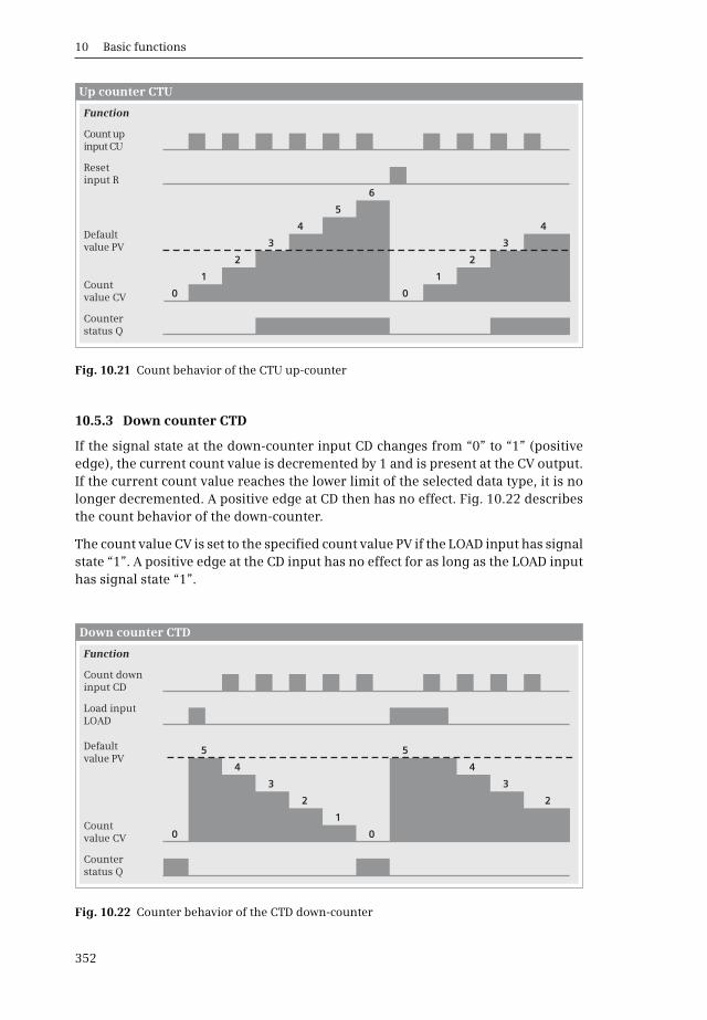
10 Basic functions
352
10.5.3 Down counter CTD
If the signal state at the down-counter input CD changes from “0” to “1” (positiveedge), the current count value is decremented by 1 and is present at the CV output.If the current count value reaches the lower limit of the selected data type, it is nolonger decremented. A positive edge at CD then has no effect. Fig. 10.22 describesthe count behavior of the down-counter.
The count value CV is set to the specified count value PV if the LOAD input has signalstate “1”. A positive edge at the CD input has no effect for as long as the LOAD inputhas signal state “1”.
Fig. 10.21 Count behavior of the CTU up-counter
Fig. 10.22 Counter behavior of the CTD down-counter
Up counter CTU
Function
Count up input CU
Reset input R
Count value CV
Default value PV
Counter status Q
0
1
2
3
4
5
6
0
1
2
3
4
Down counter CTD
Function
Count down input CD
Load inputLOAD
Count value CV
Default value PV
Counter status Q
0
1
2
3
4
5
0
5
2
3
4
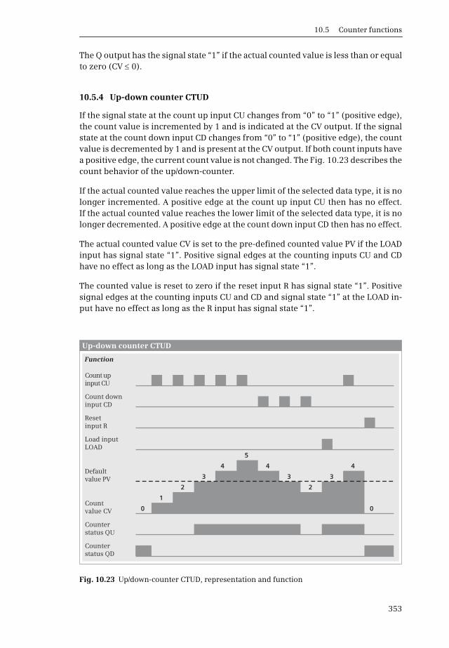
10.5 Counter functions
353
The Q output has the signal state “1” if the actual counted value is less than or equalto zero (CV 0).
10.5.4 Up-down counter CTUD
If the signal state at the count up input CU changes from “0” to “1” (positive edge),the count value is incremented by 1 and is indicated at the CV output. If the signalstate at the count down input CD changes from “0” to “1” (positive edge), the countvalue is decremented by 1 and is present at the CV output. If both count inputs havea positive edge, the current count value is not changed. The Fig. 10.23 describes thecount behavior of the up/down-counter.
If the actual counted value reaches the upper limit of the selected data type, it is nolonger incremented. A positive edge at the count up input CU then has no effect.If the actual counted value reaches the lower limit of the selected data type, it is nolonger decremented. A positive edge at the count down input CD then has no effect.
The actual counted value CV is set to the pre-defined counted value PV if the LOADinput has signal state “1”. Positive signal edges at the counting inputs CU and CDhave no effect as long as the LOAD input has signal state “1”.
The counted value is reset to zero if the reset input R has signal state “1”. Positivesignal edges at the counting inputs CU and CD and signal state “1” at the LOAD in-put have no effect as long as the R input has signal state “1”.
Fig. 10.23 Up/down-counter CTUD, representation and function
Function
Up-down counter CTUD
Count up input CU
Count down input CD
Reset input R
Load inputLOAD
Count value CV
Default value PV
Counter status QU
Counter status QD
0
1
2
3
4
5
4
3
2
3
4
0

10 Basic functions
354
The QU output has the signal state “1” if the actual counted value is greater than orequal to the defined counted value (CV PV).
The QD output has the signal state “1” if the actual counted value is less than orequal to zero (CV 0).

11 Digital functions
355
11 Digital functions
This chapter describes the digital functions which mainly link digital tags together,for example the basic arithmetic operations for the arithmetic functions. As far aspossible, the description is independent of the programming language.
The Chapters 7 “Ladder logic LAD” on page 209, 8 “Function block diagram FBD” onpage 246, and 9 “Structured Control Language SCL” on page 284 describe how youcan program the functions using the individual programming languages and whatspecial features exist.
The digital functions are implemented internally – not visible to you as the user –either by means of basic instruction sequences or by calling a system or standardblock. Therefore you can find the digital functions in the program elements catalogunder Basic instructions and Extended instructions. The following digital functionsare available with a CPU 1200:
b The transfer functions transfer the value of a (digital) tag or memory area.
b The comparison functions generate a binary result by comparing two tags.
b The arithmetic functions for numerical values link two tags with data types fixed-point and floating-point data types in accordance with the basic arithmetic operations.
b The arithmetic functions for time values link two tags with data types DTL, TOD, DATE, and TIME.
b The math functions convert the value of a tag with data type REAL or LREAL in accordance with the specified function, for example calculation with a trigono-metric function.
b The conversion functions convert the data type of a tag.
b The shift functions shift the content of a tag bit by bit to the right or left.
b The logic functions comprise, for example, the word logic operations, which link two tags bit by bit, and the selection and limiting functions.
b The functions for strings process tags with data type STRING. Two strings can be combined, for example.
b In LAD and FBD, the CALCULATE box allows a complex, user-defined logical operation with logical, arithmetic, and mathematical functions.
The “simple” digital functions are boxes in the case of LAD and FBD (with LAD, thecomparison is a contact) and arithmetic, logic and comparison expressions in thecase of SCL.

11 Digital functions
356
11.1 Transfer functions
11.1.1 Introduction
The transfer functions allow values to be exchanged between tags. The tags can alsobe overwritten with fixed values (constants). The tags – except data type BOOL – canbe of all data types; any limitations are referred to in the respective functional de-scriptions. The transfer function is executed when the EN input has signal state “1”or is unused. The ENO output has signal state “0” if the box has not been processed(EN = “0”) or if an error has occurred during box processing.
The following transfer functions are available:
b MOVE-Box, S_MOVE-BoxCopy tag content (LAD, FBD)
b Value assignmentCopy the value of a tag or of an expression (SCL)
b MOVE_BLK box Copy data area
b UMOVE_BLK boxCopy data area without interruption
b FILL_BLK box Fill the data area
b UFILL_BLK boxFill the data area without interruptions
b READ_DBL, WRIT_DBLTransfer data area from and to load memory
b SWAP box Swap bytes
The FieldRead and FieldWrite functions, which in STEP 7 V10.5 allowed field com-ponents to be addressed with a variable index, is still available in STEP 7 V11, but isno longer required. With indirect addressing of field components, there is a moreelegant way.
11.1.2 Copy tag, MOVE box for LAD and FBD
The MOVE box transfers the content of the tag at the IN parameter to the tag at theOUT1 parameter (Fig. 11.1). If there is a tag with elementary data type at parameterIN, the MOVE box can be expanded with additional outputs OUT2, OUT3, etc. usingthe command Insert output from the shortcut menu. The content of the input tag isthen transferred to all box inputs. A tag with elementary data type can also be acomponent of a structured data type.

11.1 Transfer functions
357
The tags at the parameters IN and OUT1 or OUTn can have different types of data.Which data types are allowed depends on the block attribute IEC check (Table 11.1).If the data width of the target tags is smaller than the data width of the tags atparameter IN, the higher-level bits are “cut off” and lost. If the data width of the tar-get tag is larger, the higher-level bits are filled with zeros.
The MOVE box can also transfer tags with structured data type, tags with hardwaredata type, PLC data type, system data type, and entire data blocks that are derivedfrom a data type (type data blocks). In these cases, the data types at IN and OUT1must always coincide. An extension of the box outputs (with OUT2, OUT3, etc.) isthen not possible.
11.1.3 Copy string, S_MOVE box for LAD and FBD
The S_MOVE box transfers the content of the tag at the IN parameter to the tag at theOUT parameter (Fig. 11.2). The tags are of data type STRING.
If the target tag is greater than the source tag, the source tag is transferred com-pletely to the target tag and the current length is updated.
Fig. 11.1 MOVE box, representation and function
Fig. 11.2 S_MOVE box, representation and function
DeclarationName
EN
ENO
IN
OUT1
–
–
INPUT
OUTPUT
*) see text
BOOL
BOOL
*)
*)
Enabling input
Enabling output
Source tag
First target tag
DescriptionData typeMOVE MOVE
EN EN
IN IN
ENO OUT1
OUT1 ENO
MOVE box
LAD FBD
Function:
**
The value at the IN parameter is transferred to the OUT1 parameter. If the tag at the IN parameter has an elementary data type, the number of output parameters can be increased.
DeclarationName
EN
ENO
IN
OUT
–
–
INPUT
OUTPUT
BOOL
STRING
BOOL
STRING
Source tag
Target tag
DescriptionData typeS_MOVE S_MOVE
EN EN
IN IN
ENO OUT
OUT ENO
S_MOVE box
LAD FBD
Function:The value at the IN parameter is transferred to the OUT parameter.
Enabling input
Enabling output
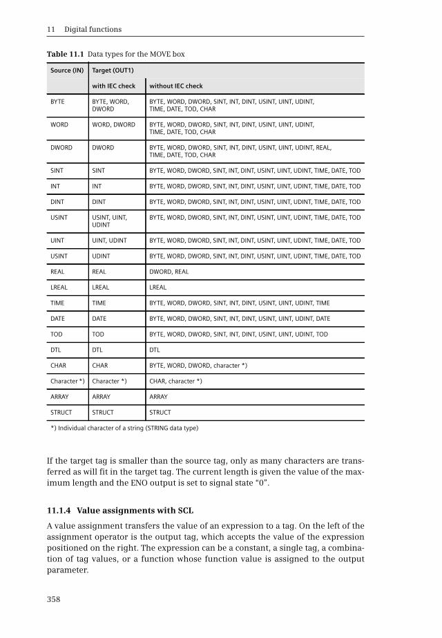
11 Digital functions
358
If the target tag is smaller than the source tag, only as many characters are trans-ferred as will fit in the target tag. The current length is given the value of the max-imum length and the ENO output is set to signal state “0”.
11.1.4 Value assignments with SCL
A value assignment transfers the value of an expression to a tag. On the left of theassignment operator is the output tag, which accepts the value of the expressionpositioned on the right. The expression can be a constant, a single tag, a combina-tion of tag values, or a function whose function value is assigned to the outputparameter.
Table 11.1 Data types for the MOVE box
Source (IN) Target (OUT1)
with IEC check without IEC check
BYTE BYTE, WORD, DWORD
BYTE, WORD, DWORD, SINT, INT, DINT, USINT, UINT, UDINT, TIME, DATE, TOD, CHAR
WORD WORD, DWORD BYTE, WORD, DWORD, SINT, INT, DINT, USINT, UINT, UDINT, TIME, DATE, TOD, CHAR
DWORD DWORD BYTE, WORD, DWORD, SINT, INT, DINT, USINT, UINT, UDINT, REAL, TIME, DATE, TOD, CHAR
SINT SINT BYTE, WORD, DWORD, SINT, INT, DINT, USINT, UINT, UDINT, TIME, DATE, TOD
INT INT BYTE, WORD, DWORD, SINT, INT, DINT, USINT, UINT, UDINT, TIME, DATE, TOD
DINT DINT BYTE, WORD, DWORD, SINT, INT, DINT, USINT, UINT, UDINT, TIME, DATE, TOD
USINT USINT, UINT, UDINT
BYTE, WORD, DWORD, SINT, INT, DINT, USINT, UINT, UDINT, TIME, DATE, TOD
UINT UINT, UDINT BYTE, WORD, DWORD, SINT, INT, DINT, USINT, UINT, UDINT, TIME, DATE, TOD
USINT UDINT BYTE, WORD, DWORD, SINT, INT, DINT, USINT, UINT, UDINT, TIME, DATE, TOD
REAL REAL DWORD, REAL
LREAL LREAL LREAL
TIME TIME BYTE, WORD, DWORD, SINT, INT, DINT, USINT, UINT, UDINT, TIME
DATE DATE BYTE, WORD, DWORD, SINT, INT, DINT, USINT, UINT, UDINT, DATE
TOD TOD BYTE, WORD, DWORD, SINT, INT, DINT, USINT, UINT, UDINT, TOD
DTL DTL DTL
CHAR CHAR BYTE, WORD, DWORD, character *)
Character *) Character *) CHAR, character *)
ARRAY ARRAY ARRAY
STRUCT STRUCT STRUCT
*) Individual character of a string (STRING data type)
11.1 Transfer functions
359
#Output_tag := #Input_tag; //Assignment of tag value
The data type of the value assignment is determined by the output tag. The datatypes on both sides of the assignment operator must be the same. Exception: Withthe IEC check block attribute deactivated, the “implicit data type conversion” isapplicable, see Chapter 4.2.3 “Absolute addressing of an operand area” on page 86.
Assignment for elementary data types
A constant value, a different tag, or an expression can be assigned to a tag or oper-and.
Absolutely addressed operands (e.g. %MW10) have one of the data types BOOL,BYTE, WORD, or DWORD. If you wish to assign a value with a different data type toan absolutely addressed operand, you can use the data type conversion or assign aname and the desired data type to the operand in the PLC tag table.
Assignment of DTL tags
Every DTL tag can be assigned another DTL tag or a DTL constant. A single compo-nent can be used like a tag with the data type of the component. Example: In the#Delivery_date tag with the DTL data type, the hour should be set:
#Delivery_date.HOUR := #Hour; //Data_type USINT
Assignment of STRING tags
Every STRING tag can be assigned another STRING tag or a STRING constant. If thesource tag is smaller than the target tag to the left of the assignment operator, allcharacters are transferred and the current length is updated. If the source tag islonger, only as many characters are transmitted as will fit in the target tag and thecurrent length is set to the maximum length.
A STRING tag can be assigned a tag with data type CHAR. Example:
#String := #Single_character;
Assignment of STRUCT tags or PLC data types
A STRUCT tag or PLC data type can only be assigned to another STRUCT tag or PLCdata type if
b the data structures agree,
b the data types of the structure components agree, and
b the names of the structure components agree.
Individual structure components can be handled like tags of the correspondingdata type, for example a structure component #Motor1.Setpoint with data type INTcan be assigned to another INT tag, or an INT value can be assigned to this struc-ture component.

11 Digital functions
360
Assignment of ARRAY tags
An ARRAY tag can only be assigned to another ARRAY tag if the data types of thearray components as well as the array limits with smallest and largest array indexagree with each other.
Individual array components can be handled like tags of the corresponding datatype. Example: If #Measured_values is a field of REAL components, and #Index is atag with the data type INT, a field component can be assigned the value of the#Width tag with data type REAL:
#Measured_values[#Index] := #Width;
11.1.5 Copy data area (MOVE_BLK, UMOVE_BLK)
MOVE_BLK and UMOVE_BLK transfer the contents of sequential components of anARRAY tag to components of another ARRAY tag. The source area is defined by thestart tag at parameter IN, and the target area by the start tag at parameter OUT. Asmany values are copied as the number specified at the COUNT parameter (Fig.11.3).
Fig. 11.3 MOVE_BLK and UMOVE_BLK box, representation and function
DeclarationName
EN
ENO
IN
COUNT
OUT
–
–
INPUT
INPUT
OUTPUT
*) see text
BOOL
BOOL
ARRAY[n] *)
*)
ARRAY[n] *)
Enabling input
Enabling output
Source tag
Number
Target tag
DescriptionData typeFunction Function
EN EN
IN IN
ENO
ENO
OUT OUT
MOVE_BLK box, UMOVE_BLK box
LAD
SCL
Funktion:
MOVE_BLKUMOVE_BLK
FBD
COUNT COUNT
Parameter IN Parameter OUT
COUNT
ARRAY tag (source) ARRAY tag (target)
Data type:
IN, OUT:
COUNT:
Function (IN := ,... COUNT := , OUT => );... ...
The contents of the source tags are trans-ferred to the ARRAY tags at the OUT para-meter into the number of components that is specified at the COUNT parameter. The component specified at the OUT para-meter is the start component for the target.
Move data areaMove data area without interruption
ARRAY[n] means a component (an element) of a tag with data type ARRAY. This component has an elementary data type.
for LAD and FBD: UINT (with activated attribute IEC check) for SCL: USINT, UINT, UDINT (with activated attribute IEC check)

11.1 Transfer functions
361
With the IEC check activated, the tags at the IN and OUT parameters must have thesame data type; if the attribute IEC check is not activated in the block, it is only nec-essary for the data widths to agree.
MOVE_BLK copies the values so that the process can be interrupted by a higher-pri-ority program (advantage: quick response time to alarms). UMOVE_BLK copieswithout interruption (advantage: transfer of consistent data areas). During transferby UMOVE_BLK, alarm events that occur are stored and processed after the transferends.
MOVE_BLK and UMOVE_BLK report an error (ENO = “0”) if a range limit is exceededduring runtime. No values are copied if an error occurs.
11.1.6 Filling the data area (FILL_BLK, UFILL_BLK)
FILL_BLK and UFILL_BLK transfer the content of a tag to sequential componentsof an ARRAY tag. The source tag is defined by parameter IN and the target area bythe start tag at parameter OUT. As many values are copied as the number specifiedat the COUNT parameter (Fig. 11.4).
Fig. 11.4 FILL_BLK and UFILL_BLK box, representation and function
DeclarationName
EN
ENO
IN
COUNT
OUT
–
–
INPUT
INPUT
OUTPUT
*) Same data width at IN and OUT
BOOL
BOOL
Data type *)
UINT
ARRAY[n] *)
DescriptionData typeFunction Function
EN EN
IN IN
ENO
ENO
OUT OUT
FILL_BLK box, UFILL_BLK box
LAD
Funktion:
FILL_BLKUFILL_BLK
FBD
COUNT COUNT
Parameter IN Parameter OUT
COUNT
Source tag
ARRAY tag (target)
SCL
Data type:
IN, OUT:
COUNT:
Function (IN := ... , COUNT := ... , OUT => ... );
Enabling input
Enabling output
Source tag
Number
Target tag
Fill data areaFill data area without interruption
The contents of the source tags are trans-ferred to the ARRAY tags at the OUT para-meter into the number of components that is specified at the COUNT parameter. The component specified at the OUT para-meter is the start component for the target.
ARRAY[n] means a component (an element) of a tag with data type ARRAY. This component has an elementary data type.
for LAD and FBD: UINT (with activated attribute IEC check) for SCL: USINT, UINT, UDINT (with activated attribute IEC check)
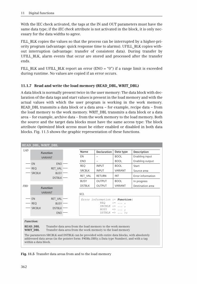
11 Digital functions
362
With the IEC check activated, the tags at the IN and OUT parameters must have thesame data type; if the IEC check attribute is not activated in the block, it is only nec-essary for the data widths to agree.
FILL_BLK copies the values so that the process can be interrupted by a higher-pri-ority program (advantage: quick response time to alarms). UFILL_BLK copies with-out interruption (advantage: transfer of consistent data). During transfer byUFILL_BLK, alarm events that occur are stored and processed after the transferends.
FILL_BLK and UFILL_BLK report an error (ENO = “0”) if a range limit is exceededduring runtime. No values are copied if an error occurs.
11.1.7 Read and write the load memory (READ_DBL, WRIT_DBL)
A data block is normally present twice in the user memory: The data block with dec-laration of the data tags and start values is present in the load memory and with theactual values with which the user program is working in the work memory.READ_DBL transmits a data block or a data area – for example, recipe data – fromthe load memory to the work memory. WRIT_DBL transmits a data block or a dataarea – for example, archive data – from the work memory to the load memory. Boththe source and the target data blocks must have the same access type: The blockattribute Optimized block access must be either enabled or disabled in both datablocks. Fig. 11.5 shows the graphic representation of these functions.
Fig. 11.5 Transfer data areas from and to the load memory
Function
VARIANT
Function
VARIANT
REQ
EN
SRCBLK
REQ
EN
SRCBLK
RET_VAL
ENO
RET_VAL
BUSY
DSTBLK
BUSY
DSTBLK
ENO
DeclarationName
EN
ENO
REQ
SRCBLK
RET_VAL
BUSY
DSTBLK
–
–
INPUT
INPUT
RETURN
OUTPUT
OUTPUT
BOOL
BOOL
BOOL
VARIANT
INT
BOOL
VARIANT
Start
Source area
Error information
In progress
Destination area
DescriptionData typeLAD
Function:
READ_DBLWRIT_DBL
Transfer data area from the load memory to the work memory
FBD
SCL
Error information...
:= (REQ := ,
Function
SRCBLK := ,BUSY => ,DSTBLK => );
...
...
...
READ_DBL, WRIT_DBL
The parameters SRCBLK and DSTBLK can be provided with entire data blocks, with absolutely addressed data areas (in the pointer form: P#DBz.DBXy.x Data type Number), and with a tag within a data block.
Transfer data area from the work memory to the load memory
Enabling input
Enabling output
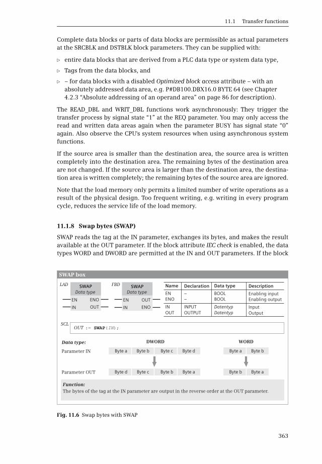
11.1 Transfer functions
363
Complete data blocks or parts of data blocks are permissible as actual parametersat the SRCBLK and DSTBLK block parameters. They can be supplied with:
b entire data blocks that are derived from a PLC data type or system data type,
b Tags from the data blocks, and
b – for data blocks with a disabled Optimized block access attribute – with an absolutely addressed data area, e.g. P#DB100.DBX16.0 BYTE 64 (see Chapter 4.2.3 “Absolute addressing of an operand area” on page 86 for description).
The READ_DBL and WRIT_DBL functions work asynchronously: They trigger thetransfer process by signal state “1” at the REQ parameter. You may only access theread and written data areas again when the parameter BUSY has signal state “0”again. Also observe the CPU's system resources when using asynchronous systemfunctions.
If the source area is smaller than the destination area, the source area is writtencompletely into the destination area. The remaining bytes of the destination areaare not changed. If the source area is larger than the destination area, the destina-tion area is written completely; the remaining bytes of the source area are ignored.
Note that the load memory only permits a limited number of write operations as aresult of the physical design. Too frequent writing, e.g. writing in every programcycle, reduces the service life of the load memory.
11.1.8 Swap bytes (SWAP)
SWAP reads the tag at the IN parameter, exchanges its bytes, and makes the resultavailable at the OUT parameter. If the block attribute IEC check is enabled, the datatypes WORD and DWORD are permitted at the IN and OUT parameters. If the block
Fig. 11.6 Swap bytes with SWAP
DeclarationName
ENENO
INOUT
––
INPUTOUTPUT
BOOLBOOL
DatentypDatentyp
DescriptionData typeSWAP SWAP
EN EN
Data type Data type
IN IN
ENO OUT
OUT ENO
SWAP box
LAD FBD
Parameter IN
Parameter OUT
Data type:
Datenbreite:
DWORD WORD
Byte c Byte a
Byte b Byte b
Byte b
Byte c
Byte a
Byte d
Byte d Byte b
Byte a Byte a
Function:The bytes of the tag at the IN parameter are output in the reverse order at the OUT parameter.
SCLOUT := (SWAP IN);
Enabling inputEnabling output
InputOutput
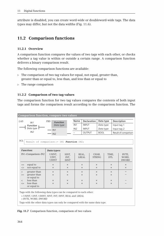
11 Digital functions
364
attribute is disabled, you can create word-wide or doubleword-wide tags. The datatypes may differ, but not the data widths (Fig. 11.6).
11.2 Comparison functions
11.2.1 Overview
A comparison function compares the values of two tags with each other, or checkswhether a tag value is within or outside a certain range. A comparison functiondelivers a binary comparison result.
The following comparison functions are available:
b The comparison of two tag values for equal, not equal, greater than, greater than or equal to, less than, and less than or equal to
b The range comparison
11.2.2 Comparison of two tag values
The comparison function for two tag values compares the contents of both inputtags and forms the comparison result according to the comparison function. The
Fig. 11.7 Comparison function, comparison of two values
DeclarationName
IN1
IN2
–
INPUT
INPUT
OUTPUT
Data type
Data type
BOOL
Input tag 1
Input tag 2
DescriptionData typeFunctionData type
IN1
LAD FBD
IN2
FunctionData type
IN1
IN2
SCL Result of comparison := IN1 IN2;Function
Comparison function, compare two values
BYTE,WORD,DWORD
Function: Data types:
USINT,UINT,UDINT
==<>
equal tonot equal to
>>=
<<=
greater than greater than or equal to less thanless than or equal to
SINT,INT,DINT
REAL,LREAL
CHAR,STRING
TIME,DTL
××
×
××
×
××
×
××
×
××
×
××
×
××
×
××
×
××
×
××
×
××
––
––
IN1 <Comparison> IN2
Tags with the following data types can be compared to each other:
> USINT, UINT, UDINT, SINT, INT, DINT, REAL and LREAL> BYTE, WORD, DWORD
Tags with the other data types can only be compared with the same data type.
Result of comparison
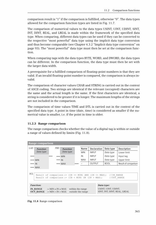
11.2 Comparison functions
365
comparison result is “1” if the comparison is fulfilled, otherwise “0”. The data typesallowed for the comparison function types are listed in Fig. 11.7.
The comparison of numerical values to the data types USINT, UINT, UDINT, SINT,INT, DINT, REAL, and LREAL is made within the framework of the specified datatype. When comparing, different data types can be used if they can be converted tothe respective “most powerful” data type using the implicit data type conversionand thus become comparable (see Chapter 4.3.2 “Implicit data type conversion” onpage 93). The “most powerful” data type must then be set at the comparison func-tion.
When comparing tags with the data types BYTE, WORD, and DWORD, the data typescan be different. In the comparison function, the data type must then be set withthe larger data width.
A prerequisite for a fulfilled comparison of floating-point numbers is that they arevalid. If an invalid floating-point number is compared, the comparison is always in-valid.
The comparison of character values CHAR and STRING is carried out in the contextof ASCII coding. Two strings are identical if the relevant (occupied) characters arethe same and the actual length is the same. If the first characters are identical, astring is considered to be greater if it is longer. The maximum lengths of the stringsare not included in the comparison.
The comparison of time values TIME and DTL is carried out in the context of thespecified data type. A point in time (date, time) is considered as smaller if the nu-merical value is smaller, i.e. if the point in time is older.
11.2.3 Range comparison
The range comparison checks whether the value of a digital tag is within or outsidea range of values defined by limits (Fig. 11.8).
Fig. 11.8 Range comparison
DeclarationName
MIN
MAX
IN
–
INPUT
INPUT
INPUT
OUTPUT
Data type
Data type
Data type
BOOL
DescriptionData type
MIN
MIN
Range comparison
IN
IN MAX
MAX
Function:
IN_RANGEOUT_RANGE
within the rangeoutside the range
:= MIN ≤ IN ≤ MAX:= MIN > IN > MAX
Data type:
USINT, UINT, UDINT,SINT, INT, DINT, REAL, LREAL
SCL Result of comparison := (IN >= MIN) AND (IN <= MAX); //IN_RANGE:= (IN < MIN) OR (IN > MAX); //OUT_RANGEResult of comparison
FunctionData type
FunctionData type
LAD FBD
Lower limit
Upper limit
Input tag
Result of comparison

11 Digital functions
366
The comparison is fulfilled (comparison result = “1”) if the digital value for thefunction IN_RANGE is within the range or if the digital value for OUT_RANGE is out-side the range. The limits (MIN, MAX) and the digital tag to be compared (IN) are atthe inputs of the box. The binary comparison result is available at the unlabeledoutput of the box.
All fixed-point and floating-point numbers are permitted as data types of the inputparameters. The data types at the input parameters can be different if they can bechanged to the “most powerful” data type with the implicit conversion and thuscompared. For different data types, the “most powerful” data type is specified in thebox.
The lower limit and upper limit may also be assigned constants. If invalid floating-point numbers are specified, the comparison is not fulfilled.
11.3 Arithmetic functions for numerical values
11.3.1 Introduction
The arithmetic functions for numerical values link two values according to thebasic arithmetical operations addition, subtraction, multiplication, and division(Fig. 11.9). The arithmetic functions include absolute value generation, changingthe sign (negation), and changing the value by 1 (decrementing, incrementing).
LAD and FBD: An arithmetic function is executed if the enable input EN is not con-nected, or if “1” is present at the enable input, or if “current” flows into the enable
Fig. 11.9 Arithmetic functions for numerical values, representation and function
EN EN
OUT OUT
ENO
ENO
Arithmetic functions for numerical values
IN1 IN1
IN2 IN2
Function:
LAD/FBD SCL
ADD + AdditionSUB – SubtractionMUL * MultiplicationDIV / DivisionMOD MOD Division with remainder as result
Data type: USINT, UINT, UDINT,SINT, INT, DINT
REAL, LREAL (not with MOD)
Name
EN
ENO
IN1
IN2
OUT
–
–
INPUT
INPUT
OUTPUT
BOOL
BOOL
Data type
Data type
Data type
SCL OUT := IN1 IN2;Function
Declaration
Enabling input
Enabling output
Input tag 1
Input tag 2
Result
DescriptionData typeData type Data typeFunction FunctionLAD FBD
If different data types are specified, the result adopts the “most powerful” data type.
11.3 Arithmetic functions for numerical values
367
input. If an error occurs during calculation, the enable output ENO is set to “0”, oth-erwise to “1”. If the execution of the function is not enabled (EN = “0”), the calcula-tion does not take place and ENO is also “0”.
SCL: The basic arithmetical operations are implemented with an arithmetic expres-sion in which two or more tags are linked. The result of an arithmetic expressioncan in turn be used in another arithmetic expression. If, during the execution of anarithmetic function, an error such as exceeding a number range occurs, the ENOtag is set to FALSE (signal state “0”).
11.3.2 Addition ADD
The ADD function interprets the values present at the IN1 and IN2 inputs as num-bers with the specified data type. It adds the two numbers, and saves the total at theOUT output. Leaving the permissible range is reported by ENO = “0”.
Floating-point addition: with an impermissible calculation (one of the input valuesis an invalid floating-point number, or you attempt to add + and -), ADD deliversan invalid value at the OUT output and sets ENO to “0”.
11.3.3 Subtraction SUB
The SUB function interprets the values present at the IN1 and IN2 inputs as num-bers with the specified data type. It subtracts the value at IN2 from the value at IN1,and saves the difference at the OUT output. Leaving the permissible range is report-ed by ENO = “0”.
Floating-point subtraction: with an impermissible calculation (one of the input val-ues is an invalid floating-point number, or you attempt to subtract + from + or - from - ), SUB delivers an invalid value at the OUT output and sets ENO to “0”.
11.3.4 Multiplication MUL
The MUL function interprets the values present at the IN1 and IN2 inputs as num-bers with the specified data type. It multiplies the two numbers, and saves the prod-uct at the OUT output. Leaving the permissible range is reported by ENO = “0”.
Floating-point multiplication: In an unauthorized calculation (one of the input val-ues is an invalid floating point number, or you try to multiply with 0), MUL sup-plies an invalid value at OUT and sets ENO to “0”.
11.3.5 Division DIV
Fixed-point division: the DIV function interprets the values present at the IN1 andIN2 inputs as numbers with the specified data type. It divides the value at input IN1(dividend) by the value at input IN2 (divisor) and delivers the quotient at theOUT output. This is the integer result of the division. The quotient is zero if the div-idend is equal to zero and the divisor is not equal to zero, or if the value of the div-

11 Digital functions
368
idend is smaller than the value of the divisor. The quotient is negative if the divisoris negative. A division by zero delivers a value of zero as the quotient, and sets ENOto “0”.
Floating-point division: the value at the IN1 parameter is divided by the value at theIN2 parameter, and the result output at the OUT parameter. With an impermissiblecalculation (one of the input values is an invalid floating-point number, or you at-tempt to divide by or 0 by 0), DIV delivers an invalid value at the OUT outputand sets ENO to “0”.
11.3.6 Division with remainder as result MOD
The MOD function interprets the values present at the IN1 and IN2 inputs as numberswith the specified data type. It divides the value at input IN1 (dividend) by the value atinput IN2 (divisor) and saves the remainder of the division at the OUT output. Theremainder refers to the remaining part of the division, and does not correspond to thedecimal positions. With a negative dividend, the remainder is also negative.
A division by zero delivers a value of zero as the remainder, and sets ENO to “0”.The MOD function does not allow tags of data type REAL or LREAL.
11.3.7 Generation of absolute value ABS
The ABS function generates the absolute value from the number at the IN parame-ter and outputs the result at the OUT parameter. With a floating-point number, thesign of the mantissa is set to “0”, even if the number is invalid.
If the allowed number range is exceeded, for example ABS(–128) for data typeSINT, or for a valid floating-point number, the ENO output has signal state “0”(Fig. 11.10).
Fig. 11.10 Absolute value generation and negation, representation and function
EN ENOUT
OUTENOENO
Generation of absolute value, negation
IN IN
Function:
ABSNEG
Generation of absolute valueNegation
Data type:
SINT, INT, DINT, REAL, LREAL
DeclarationName
EN
ENO
IN
OUT
–
–
INPUT
OUTPUT
BOOL
BOOL
Data type
Data type
DescriptionData type
SCL OUT := ABS(IN1); //Generation of absolute valueOUT := -IN; //Negation (two's complement)
Enabling input
Enabling output
Input tag
Result
LAD FBDFunctionData type
FunctionData type

11.4 Arithmetic functions for time values
369
11.3.8 Negation NEG
The NEG function reverses the sign of the number at the IN parameter and outputsthe result at the OUT parameter. The negation is equivalent to a multiplication by –1. With a floating-point number, the sign of the mantissa is changed, even if the num-ber is invalid (Fig. 11.10).
If the result is out of the valid number range, e.g .NEG(–128) for the data type SINT,the enable output ENO is set to signal state “0”.
11.3.9 Decrement DEC, increment INC
The function DEC (decrement) reduces the value at the IN/OUT parameter by 1 as ina subtraction. The function INC (increment) increases the value at the IN/OUTparameter by 1 as in an addition (Fig. 11.11).
LAD, FBD: When reaching the lowest and highest numerical value for the data type,the enable output ENO is set to signal state “0”.
SCL: If the allowed number range is exceeded, the ENO tag is set to FALSE (signalstate “0”).
11.4 Arithmetic functions for time values
11.4.1 Introduction
The arithmetic functions for time values link durations (data type TIME) and pointsin time (data type DTL) together.
An arithmetic function is executed if the enable input EN is not connected, or if “1”is present at the enable input, or if “current” flows into the enable input. If an error
Fig. 11.11 Decrementing and incrementing, representation and function
EN ENENOENO
Decrementing, incrementing
IN/OUT IN/OUT
Function:
DECINC
DecrementIncrement
Data type:
SINT, INT, DINT, USINT, UINT, UDINT
DeclarationName
ENENO
IN/OUT
––
INOUT
BOOLBOOL
Datentyp
DescriptionData type
SCL Variable Variable:= + 1; //IncrementingVariable Variable:= - 1; //Decrementing
LAD FBDFunctionData type
FunctionData type Enabling input
Enabling output
Digital tag
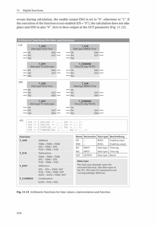
11 Digital functions
370
occurs during calculation, the enable output ENO is set to “0”, otherwise to “1”. Ifthe execution of the function is not enabled (EN = “0”), the calculation does not takeplace and ENO is also “0”. Zero is then output at the OUT parameter (Fig. 11.12).
Fig. 11.12 Arithmetic functions for time values, representation and function
Function:
Addition
TIME + TIME = TIMEDTL + TIME = DTLTOD + TIME = TOD
Subtraction
TIME – TIME = TIMEDTL TIME = DTLTOD – TIME = TOD
T_ADD
T_SUB
–
Difference
DTL – DTL = TIME / INTTOD – TOD = TIME / INTDATE – DATE = TIME / INT
Combination
DATE + TOD = DTL
T_DIFF
T_COMBINE
Data type:
EN
EN
EN
EN
EN
EN
EN
EN
ENO
ENO
ENO
ENO
ENO
ENO
ENO
ENO
OUT
OUT
OUT
OUT
OUT
OUT
OUT
OUT
Arithmetic functions for date and duration
LAD
FBD
IN1
IN1
IN1
IN1
IN1
IN1
IN1
IN1
IN2
IN2
IN2
IN2
IN2
IN2
IN2
IN2
DeclarationName
EN
ENO
IN1
IN2
OUT
–
–
INPUT
INPUT
OUTPUT
BOOL
BOOL
Data type
Data type
Data type
BeschreibungData type
T_ADDData type PLUS Time
T_ADDData type PLUS Time
T_DIFFData type Data typeTO
T_DIFFData type Data typeTO
T_SUBData type MINUS Time
T_SUBDatentyp MINUS Time
T_COMBINETime_Of_Day TO DTL
T_COMBINETime_Of_Day TO DTL
SCLOUT := T_ADD(IN1 := ... , IN2 := ... );OUT := T_SUB(IN1 := ... , IN2 := ... );OUT := T_DIFF(IN1 := ..., IN2 := ... );OUT := T_COMBINE(IN1 := ... , IN2 := ... );
Enabling input
Enabling output
Time tag
Time tag
Result
The data type depends upon the executed function. The data types at the IN1, IN2 and OUT parameters are correspondingly different.

11.4 Arithmetic functions for time values
371
The following errors can occur with an arithmetic function for time values:
b Invalid bit assignment for DTL
b Violation of permissible range of values for TIME or DTL
11.4.2 Addition T_ADD
The T_ADD function adds the values at the IN1 and IN2 parameters and applies theresult to the OUT parameter. The parameters have different data types dependingon the calculation:
b Addition of two durations TIME + TIME = TIME
b Addition of a duration to a point in time DTL + TIME = DTL
b Addition of a duration to the time of day TOD + TIME = TOD
T_ADD sets ENO to “0” when the permissible range of values is violated. The resultis limited to the permissible range.
11.4.3 Subtraction T_SUB
The T_SUB function subtracts the value at the IN2 parameter from the value at theIN1 parameter and applies the result to the OUT parameter. The parameters havedifferent data types depending on the calculation:
b Subtraction of two durations TIME – TIME = TIME
b Subtraction of a duration from a point in time DTL – TIME = DTL
b Subtraction of a duration from a time of day TOD – TIME = TOD
T_SUB sets ENO to “0” when the permissible range of values is violated. The resultis limited to the permissible range.
11.4.4 Difference T_DIFF
The function T_DIFF subtracts the value at the IN2 parameter from the value at IN1parameter and stores the result at the OUT parameter. The difference between twopoints in time (DTL, TOD, or DATE) is formed. The result is available in the data typeTIME or INT.
T_DIFF sets ENO to “0” when the permissible range of values is violated. The resultis limited to the permissible range.
11.4.5 Combine T_COMBINE
The T_COMBINE function summarizes tags together with data types DATE andTIME_OF_DAY (TOD), converts the data type to DATE_AND_TIME (DTL), and returnsthe value at the OUT parameter.
The statement does not report any errors.

11 Digital functions
372
11.5 Mathematical functions
11.5.1 Introduction
The following mathematical functions are available:
b Trigonometric functions: sine (SIN), cosine (COS), tangent (TAN)
b Arc functions: arc sine (ASIN), arc cosine (ACOS), arc tangent (ATAN)
b Generation of square (SQR) and square root (SQRT)
b Exponential function to base e (EXP) and to any base (EXPT)
b Napierian logarithm (LN)
b Extract decimal places (FRAC)
All mathematical functions process floating-point numbers.
Fig. 11.13 Mathematical functions, representation and function
EXPTDT1 DT2**
EXPTDT1 DT2**
EN
EN
EN
EN
OUT
OUT
OUTENO
ENO
ENO
OUT
ENO
Mathematical functions
Exponentiate to any base EXPT
LAD FBD
IN
IN1
IN2
IN
IN1
IN2
Function: SINCOSTAN
SineCosineTangent
ASINACOSATAN
SQR EXPSQRT LN
FRAC
Arc sineArc cosineArc tangent
Formation of square Exponential function to base eExtraction of square root Natural logarithm
Decimal places
Data type 1: REAL, LREAL
Data type 2: USINT, UINT, UDINT, SINT, INT, DINT,REAL, LREAL
Declaration
Declaration
Name
Name
EN
EN
ENO
ENO
IN
IN1
OUT
IN2
OUT
–
–
–
–
INPUT
INPUT
OUTPUT
INPUT
OUTPUT
BOOL
BOOL
BOOL
BOOL
REAL, LREAL
Data type 1
REAL, LREAL
Data type 2
Data type 1
Description
Description
Data type
Data type
Function: EXPT Exponential function to any base
SCL
SCL
OUT := (IN);Function
OUT := IN1 IN2;**
Enabling input
Enabling output
Digital tag
Result
Enabling input
Enabling output
Base
Exponent
Result
FunctionData type
FunctionData type
LAD FBD

11.5 Mathematical functions
373
A mathematical function is executed if the enabling input EN is unused or if “1” ispresent at the enabling input (“current” flows into the enabling input). If an erroroccurs during the calculation, the enabling output ENO is set to “0”, otherwise to“1”. The calculation is not carried out if it has not been enabled (EN = “0”), and ENOis also “0”.
11.5.2 Trigonometric functions SIN, COS, TAN
The trigonometric functions generate the sine (SIN), cosine (COS) or tangent (TAN)of the tag at the IN parameter and output it at the OUT parameter. An angle speci-fied in radians as a floating-point number is expected at the IN parameter.
Two units are common for the magnitude of an angle: degrees from 0° to 360° andradians from 0 to 2 (where = +3.141593e+00). Either can be converted propor-tionally. For example, the radian measure for a 90° angle is /2, i.e. +1.570796e+00.With values greater than 2 (+6.283185e+00), 2 or a multiple thereof is subtractedfrom this until the input value for the trigonometric function is less than 2.
The enabling output ENO is set to signal state “0” when an invalid floating-pointnumber, + or – is present at the IN parameter. The value of IN is then output atthe OUT parameter.
11.5.3 Arc functions ASIN, ACOS, ATAN
The arc functions generate the arc sine (ASIN), arc cosine (ACOS) or arc tangent (ATAN)of the tags the IN parameter and output the result at the OUT parameter. They are theinverted functions of the respective trigonometric function. They expect a floating-point number within a certain range at the IN input, and return an angle in radians(Table 11.2).
The signal state “0” is set at the enabling output ENO if the value at the IN parame-ter is not in the range 1 (with ASIN or ACOS) or if an invalid floating-point numberis present at the IN parameter. An invalid floating-point number is then output atthe OUT parameter.
Table 11.2 Range of arc functions
Function Permissible range Returned value
Arc sine ASIN –1 to +1 –/2 to +/2
Arc cosine ACOS –1 to +1 0 to
Arc tangent ATAN Complete range –/2 to +/2

11 Digital functions
374
11.5.4 Formation of square SQR
The SQR function forms the square of the value present at the IN input and appliesthe result to the OUT output.
The enabling output ENO is set to signal state “0” if the value at the IN parameteror the result of the calculation is an invalid floating-point number. In the first case,an invalid floating-point number is output at the OUT parameter, and in the secondcase +.
11.5.5 Extraction of square root SQRT
The SQRT function extracts the square root of the value present at the IN input andapplies the result to the OUT output.
If a value less than zero is present at the IN input, SQRT returns an invalid floating-point number. If the value at the IN input is an invalid floating-point number or ±,the invalid floating-point number or ± is output at OUT. The enabling output ENOis set to signal state “0” in both cases.
11.5.6 Exponentiate to base e EXP
The EXP function calculates the power from base e (= 2.718282e+00) and the valuepresent at the IN input, and applies the result to the OUT output.
The enabling output ENO is set to signal state “0” if the value at the IN parameteror the result of the calculation is an invalid floating-point number. In the first case,an invalid floating-point number is output at the OUT parameter, and in the secondcase +.
11.5.7 Calculation of Napierian logarithm LN
The LN function calculates the Napierian logarithm to base e (= 2.718282e+00) ofthe number present at the IN input and applies the result to the OUT output.
The enabling output ENO is set to signal state “0” if:
b The value at the IN1 parameter is zero, negative, – or a negative, invalid float-ing-point number. – is then output at the OUT parameter.
b The value at the IN1 parameter is + or a positive, invalid floating-point number.The value of IN1 is then output at the OUT parameter.
The Napierian logarithm is the inverted function of the exponential function: If y = ex, then x = ln y.
OUT IN 2=
OUT IN=
OUT eIN=
OUT IN ln=
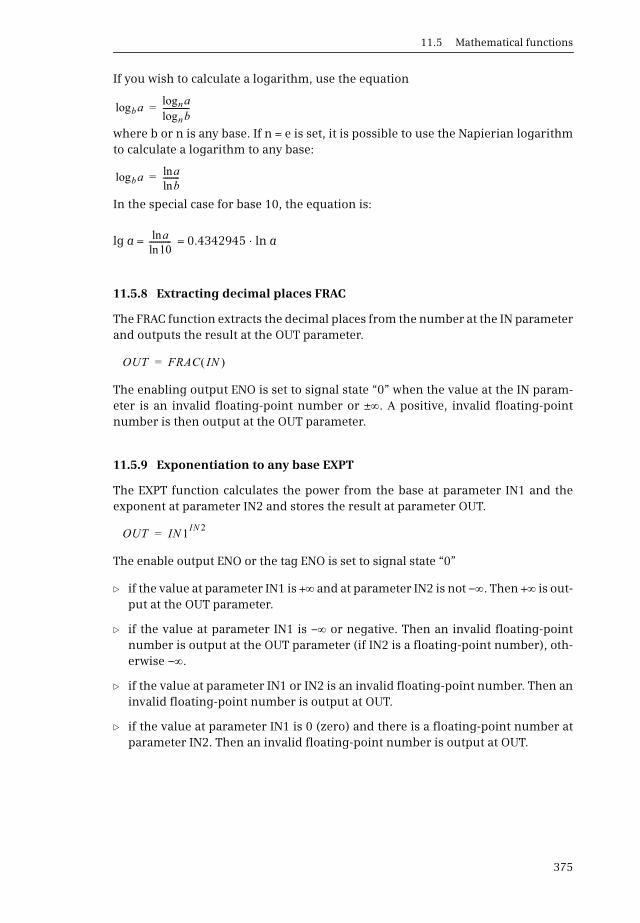
11.5 Mathematical functions
375
If you wish to calculate a logarithm, use the equation
where b or n is any base. If n = e is set, it is possible to use the Napierian logarithmto calculate a logarithm to any base:
In the special case for base 10, the equation is:
lg a = = 0.4342945 · ln a
11.5.8 Extracting decimal places FRAC
The FRAC function extracts the decimal places from the number at the IN parameterand outputs the result at the OUT parameter.
The enabling output ENO is set to signal state “0” when the value at the IN param-eter is an invalid floating-point number or ±. A positive, invalid floating-pointnumber is then output at the OUT parameter.
11.5.9 Exponentiation to any base EXPT
The EXPT function calculates the power from the base at parameter IN1 and theexponent at parameter IN2 and stores the result at parameter OUT.
The enable output ENO or the tag ENO is set to signal state “0”
b if the value at parameter IN1 is + and at parameter IN2 is not –. Then + is out-put at the OUT parameter.
b if the value at parameter IN1 is – or negative. Then an invalid floating-pointnumber is output at the OUT parameter (if IN2 is a floating-point number), oth-erwise –.
b if the value at parameter IN1 or IN2 is an invalid floating-point number. Then aninvalid floating-point number is output at OUT.
b if the value at parameter IN1 is 0 (zero) and there is a floating-point number atparameter IN2. Then an invalid floating-point number is output at OUT.
balog nalognblog
-------------=
balog alnbln
--------=
aln10ln
-----------
OUT FRAC IN =
OUT IN 1IN 2=
11 Digital functions
376
11.6 Conversion functions (Conversion of data type)
11.6.1 Introduction
If you link tags together, they must have the same data type. This also applies if youassign values or supply function or block parameters. If a tag is not available in therequired data type, the data type must be converted. The “simple” conversion func-tions are available for this.
With the “extended” conversion functions, for example, a number available inSTRING format can be converted into a number format or a character sequence intoa number sequence. The “extended” conversion functions are usually based on asystem or standard block.
The following conversion functions are available:
b CONVConversion of bit sequences (BYTE, WORD, DWORD) and numerical types (SINT, INT, DINT, USINT, UINT, UDINT, REAL, LREAL) among themselves, conversion of INT to BCD16 and vice versa, conversion of DINT to BCD32 and vice versa
b ROUND, FLOOR, CEIL, TRUNCConversion of floating-point numbers (REAL, LREAL) into floating-point and fixed-point numbers (SINT, INT, DINT, USINT, UINT, UDINT, REAL, LREAL)
b SCALE_X, NORM_XConversion (scaling) of floating-point numbers (REAL) to floating-point and fixed-point numbers (SINT, INT, DINT, USINT, UINT, UDINT, REAL) and conversion (standardization) of floating-point and fixed-point numbers (SINT, INT, DINT, USINT, UINT, UDINT, REAL) to floating-point numbers (REAL)
b T_CONVConversion of a duration (TIME) into a fixed-point number (DINT) and vice versa
b S_CONVConversion of floating-point and fixed-point numbers (SINT, INT, DINT, USINT, UINT, UDINT, REAL) into a string (STRING) and vice versa and copying of a string (STRING)
b STRG_VAL, VAL_STRGConversion of floating-point and fixed-point numbers (SINT, INT, DINT, USINT, UINT, UDINT, REAL) into a string (STRING) and vice versa with specification of notation
b Strg_TO_Chars, Chars_TO_StrgConversion of a string (STRING) to a character array (ARRAY OF CHAR) and vice versa
b ATH, HTAConversion of a character sequence in ASCII format into a number sequence in hexadecimal format, and vice versa
11.6 Conversion functions (Conversion of data type)
377
Execution of a conversion function
LAD and FBD: The conversion function is executed if the signal state “1” is presentat enable input EN (if “current” is flowing into the enable input) or if the enableinput remains unconnected. If an error occurs during conversion, the enable out-put ENO is set to “0”, otherwise to “1”. If the execution of the function is not enabled(EN = “0”), the conversion does not take place and ENO is also “0”.
SCL: If an error occurs when processing a conversion function, the tag ENO is resetto signal state “0”.
These conversion functions are “explicit” conversion functions, where the bitassignments of the tags change or where conversion errors can occur, for examplea conversion from DINT to REAL. These conversions must be programmed.“Implicit” conversion functions also exist which convert a data type without chang-ing the bit assignments and do not signal an error, for example the conversion fromBYTE to WORD. These conversions are carried out “automatically”. Further detailscan be found in Chapter 4.3.2 “Implicit data type conversion” on page 93.
11.6.2 Conversion function CONV
Conversion function CONV for fixed-point numbers and bit sequences
The conversion function CONV converts the data type of the tags at parameter IN toanother and outputs the result at the OUT parameter.
When setting BYTE, WORD or DWORD, a constant (at the IN parameter) or a tag withelementary data type can be specified which has the set data width (8, 16 or 32 bits).
The numerical value of the tag at the IN parameter is transferred right-justified to thetag at the OUT parameter. If “vacant” digits result because the data types have differ-ent lengths, they are padded with the sign. If the permissible numerical range at theOUT parameter is exceeded during the conversion, ENO is set to signal state “0”.
Conversion function CONV for BCD numbers
The conversion function CONV converts a fixed-point number at the IN parameterinto a BCD number and vice versa. The result is available at the OUT parameter.
Conversion of INT to BCD16 or of DINT to BCD32
The value at parameter IN is converted to a BCD-coded number with three (BCD16)or seven (BCD32) decades at parameter OUT. The right-justified decades representthe absolute value of the decimal number. The sign is located in the bits 12 to 15(BCD16) or 28 to 31 (BCD32). If bit 15 or 31 is set to signal state “0”, the sign is pos-itive; bit 15 or bit 31 set to signal state “1” indicates a negative sign. If the numberis too large for a conversion into a BCD number, the conversion function sets ENOto “0”. The conversion is not carried out in this case.

11 Digital functions
378
Conversion of BCD16 to INT or of BCD32 to DINT
The value at the IN parameter is converted into a fixed-point number at the OUT pa-rameter. If the number is too large for conversion to a fixed-point number with thecorresponding data type, the conversion function sets ENO to “0”. The conversionis not carried out in this case.
11.6.3 Conversion functions for floating-point numbers
The conversion function CONV converts fixed-point numbers into floating-pointnumbers and vice versa. For conversion from floating-point numbers into fixed-point numbers, there are additional features that differ in rounding behavior(Table 11.3). If an error occurs during conversion, no conversion takes place.
Fig. 11.14 Conversion function CONV, representation and function
CONVDT1 to DT2
EN EN
OUT
OUTENO
ENO
Conversion function CONV
LAD FBD
IN IN
DeclarationName
EN
ENO
IN
OUT
–
–
INPUT
OUTPUT
BOOL
BOOL
Data type 1
Data type 2
DescriptionData typeCONVDT1 to DT2
Function:
The following data type combinations are possible:
Data type conversion for from Data type DT1 to Data type DT2
BYTE, WORD, DWORD,BYTE, WORD, DWORD USINT, UINT, UDINT,
SINT, INT, DINT
USINT, UINT, UDINT,USINT, UINT, UDINT, SINT, INT, DINT,SINT, INT, DINT BYTE, WORD, DWORD,
REAL, LREAL
INT BCD16DINT BCD32BCD16 INTBCD32 DINT
USINT, UINT, UDINT,REAL, LREAL SINT, INT, DINT,
REAL, LREAL
SCL OUT := (IN);DT1_TO_DT2
Bit sequences
Fixed-point numbers
BCD numbers
Floating-point numbers
Enabling input
Enabling output
Input tag
Output tag
The conversion function CONV is used to convert data types. The content of the tag with data type DT1 at the IN parameter is converted and transferred to the tag with data type DT2 at the OUT parameter.

11.6 Conversion functions (Conversion of data type)
379
Conversion of fixed-point numbers into floating-point numbers with the CONV function
The conversion function CONV converts a fixed-point number (SINT, INT, DINT,US-INT, UINT, UDINT) at the IN parameter into a floating-point number (REAL,LREAL) and outputs the result at the OUT parameter. If the accuracy suffers duringthe conversion of DINT or UDINT into REAL, ENO is set to “0”.
Conversion of floating-point numbers into fixed-point numbers with the CONV function
The conversion function CONV converts a floating-point number at the IN parame-ter (REAL, LREAL) into a fixed-point number (SINT, INT, DINT, USINT, UDINT) andoutputs the result at the OUT parameter. During conversion figures are rounded tothe next integer. ENO is set to “0” if during conversion the allowed number range isexceeded or an invalid floating-point number is specified.
Conversion of REAL into LREAL and vice versa with the CONV function
The conversion function CONV converts a floating-point number at the IN parame-ter into a floating-point number with a different data type (REAL to LREAL or LREALto REAL) and outputs the result at the OUT parameter. ENO is set to “0” if the per-missible numerical range is violated during the conversion or if an invalid floating-point number is specified.
Conversion of REAL into fixed-point number with the CEIL function
The conversion function CEIL converts the data type REAL or LREAL of the tag atthe IN parameter into a fixed-point data type, and outputs the result at the OUT pa-rameter. During the conversion, CEIL rounds-off to the next largest integer. ENO isset to “0” if the permissible numerical range is violated during the conversion or ifan invalid floating-point number is specified.
Table 11.3 Conversion of floating-point numbers
Function Conversion
CONV Conversion from USINT, UINT, UDINT, SINT, INT or DINT to REAL or LREAL
Conversion from REAL or LREAL to USINT, UINT, UDINT, SINT, INT or DINT
CONV With rounding to the next integer (as ROUND)
CEIL With rounding to the next higher integer
FLOOR With rounding to the next smaller integer
ROUND With rounding to the next integer
TRUNC Without rounding
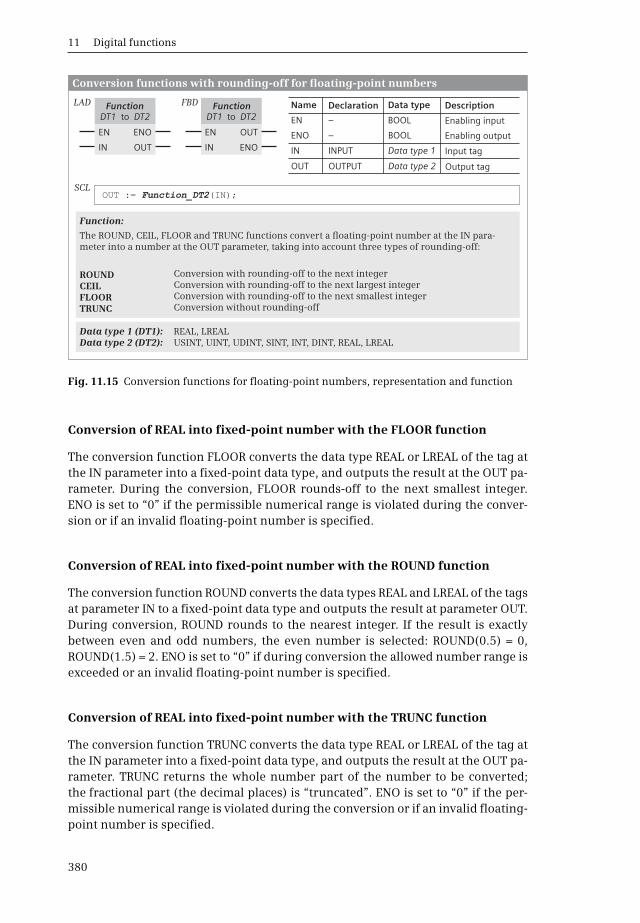
11 Digital functions
380
Conversion of REAL into fixed-point number with the FLOOR function
The conversion function FLOOR converts the data type REAL or LREAL of the tag atthe IN parameter into a fixed-point data type, and outputs the result at the OUT pa-rameter. During the conversion, FLOOR rounds-off to the next smallest integer.ENO is set to “0” if the permissible numerical range is violated during the conver-sion or if an invalid floating-point number is specified.
Conversion of REAL into fixed-point number with the ROUND function
The conversion function ROUND converts the data types REAL and LREAL of the tagsat parameter IN to a fixed-point data type and outputs the result at parameter OUT.During conversion, ROUND rounds to the nearest integer. If the result is exactlybetween even and odd numbers, the even number is selected: ROUND(0.5) = 0,ROUND(1.5) = 2. ENO is set to “0” if during conversion the allowed number range isexceeded or an invalid floating-point number is specified.
Conversion of REAL into fixed-point number with the TRUNC function
The conversion function TRUNC converts the data type REAL or LREAL of the tag atthe IN parameter into a fixed-point data type, and outputs the result at the OUT pa-rameter. TRUNC returns the whole number part of the number to be converted;the fractional part (the decimal places) is “truncated”. ENO is set to “0” if the per-missible numerical range is violated during the conversion or if an invalid floating-point number is specified.
Fig. 11.15 Conversion functions for floating-point numbers, representation and function
DT1 DT2to
EN EN
OUT
OUTENO
ENO
Conversion functions with rounding-off for floating-point numbers
IN IN
Function:
ROUNDCEILFLOORTRUNC
Data type 1 (DT1): REAL, LREALUSINT, UINT, UDINT, SINT, INT, DINT, REAL, LREAL
DeclarationName
EN
ENO
IN
OUT
–
–
INPUT
OUTPUT
BOOL
BOOL
Data type 1
Data type 2
Enabling input
Enabling output
DescriptionData typeDT1 DT2to
SCLOUT := (IN);Function_DT2
Input tag
Output tag
FunctionLAD FBD Function
The ROUND, CEIL, FLOOR and TRUNC functions convert a floating-point number at the IN para-meter into a number at the OUT parameter, taking into account three types of rounding-off:
Conversion without rounding-off
Conversion with rounding-off to the next integerConversion with rounding-off to the next largest integerConversion with rounding-off to the next smallest integer
Data type 2 (DT2):

11.6 Conversion functions (Conversion of data type)
381
Overview of rounding-off when converting floating-point into fixed-point
Table 11.4 shows the different effects of rounding when converting floating pointto fixed point using the example of the REAL data type in the range between -1 and+1.
11.6.4 Conversion functions SCALE_X and NORM_X
Scaling SCALE_X
The function SCALE_X maps the floating-point number at the VALUE parameter inthe value range of 0.0 to 1.0 to a range of values defined by the range limits at theparameters MIN and MAX. The result is output at the OUT parameter (Fig. 11.16).
Please note: The value applied at the VALUE parameter must be within the limitsof 0 and 1 (inclusive)! If this is not the case, the value at the OUT parameter may besmaller than MIN or greater than MAX. If it is still within the range permissible forthis data type, SCALE_X does not signal an error (ENO = “1”).
The function SCALE_X reports an error (ENO = “0”) if there is an invalid floating-point number at the VALUE parameter (VALUE is then written to the OUT parame-ter), if the result is outside the range of validity of the data type at the OUT param-
Table 11.4 Types of rounding for converting REAL numbers
Input value Result as fixed-point number
REAL 16# ROUND CEIL FLOOR TRUNC
1.0000001 3F80 0001 1 2 1 1
1.0 3F80 0000 1 1 1 1
0.99999995 3F7F FFFF 1 1 0 0
0.50000005 3F00 0001 1 1 0 0
0.5 3F00 0000 0 1 0 0
0.49999996 3EFF FFFF 0 1 0 0
5.877476E–39 0080 0000 0 1 0 0
0.0 0000 0000 0 0 0 0
–5.877476E–39 8080 0000 0 0 –1 0
–0.49999996 BEFF FFFF 0 0 –1 0
–0.5 BF00 0000 0 0 –1 0
–0.50000005 BF00 0001 –1 0 –1 0
–0.99999995 BF7F FFFF –1 0 –1 0
–1.0 BF80 0000 –1 –1 –1 –1
–1.0000001 BF80 0001 –1 –1 –2 –1

11 Digital functions
382
eter and the value at the MAX parameter is less than or equal to that at the MINparameter (in both cases, OUT is assigned without definition).
Normalizing NORM_X
The NORM_X function normalizes the number at the VALUE parameter to therange 0 to 1, based on a value range specified with the MIN and MAX parameters,and returns it as a REAL number at the OUT parameter (Fig. 11.16).
Please note: The value applied at the VALUE parameter must be within the limits ofMIN and MAX (inclusive)! If this is not the case, the value at the OUT parameter may
Fig. 11.16 SCALE_X and NORM_X functions, representation and function
SCALE_XREAL to DT
SCALE_XREAL to DT
EN
VALUE
EN
VALUE
OUT
OUT
ENO
ENO
Scaling SCALE_X
LAD FBD
MIN
MAX
MIN
MAX
Data type:
USINT, UINT, UDINT,SINT, INT, DINT,REAL, LREAL
DeclarationName
EN
ENO
MIN
VALUE
MAX
OUT
–
–
INPUT
INPUT
INPUT
OUTPUT
BOOL
BOOL
Data type
REAL, LREAL
Data type
Data type
DescriptionData type
OUT := VALUE (MAX – MIN) + MIN0 VALUE 1
Function:
NORM_Xto REALDT
NORM_Xto REALDT
EN
VALUE
EN
VALUE
OUT
OUT
ENO
ENO
Standardization NORM_X
LAD FBD
MIN
MAX
MIN
MAX
DeclarationName
EN
ENO
MIN
VALUE
MAX
OUT
–
–
INPUT
INPUT
INPUT
OUTPUT
BOOL
BOOL
Data type
Data type
Data type
REAL, LREAL
DescriptionData type
Data type:
USINT, UINT, UDINT,SINT, INT, DINT,REAL, LREAL
Function:
OUT := (VALUE – MIN) / (MAX MIN)–0 OUT 1
SCL
SCL
OUT := (MIN := ... , VALUE := ... , MAX := ... );SCALE_X_Data type
OUT := (MIN := ... , VALUE := ... , MAX := ... );NORM_X_Data type
Enabling input
Enabling output
Lower limit
Input tag
Upper limit
Result
The value of the tag at the VALUE parameter is converted linearly between the MIN and MAX limits, and output at the OUT parameter.
Enabling input
Enabling output
Lower limit
Input tag
Upper limit
Result
The value of the tag at the VALUE parameter is converted linearly between the MIN and MAX limits, and output at the OUT parameter.
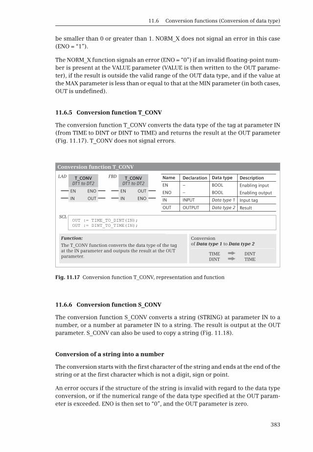
11.6 Conversion functions (Conversion of data type)
383
be smaller than 0 or greater than 1. NORM_X does not signal an error in this case(ENO = “1”).
The NORM_X function signals an error (ENO = “0”) if an invalid floating-point num-ber is present at the VALUE parameter (VALUE is then written to the OUT parame-ter), if the result is outside the valid range of the OUT data type, and if the value atthe MAX parameter is less than or equal to that at the MIN parameter (in both cases,OUT is undefined).
11.6.5 Conversion function T_CONV
The conversion function T_CONV converts the data type of the tag at parameter IN(from TIME to DINT or DINT to TIME) and returns the result at the OUT parameter(Fig. 11.17). T_CONV does not signal errors.
11.6.6 Conversion function S_CONV
The conversion function S_CONV converts a string (STRING) at parameter IN to anumber, or a number at parameter IN to a string. The result is output at the OUTparameter. S_CONV can also be used to copy a string (Fig. 11.18).
Conversion of a string into a number
The conversion starts with the first character of the string and ends at the end of thestring or at the first character which is not a digit, sign or point.
An error occurs if the structure of the string is invalid with regard to the data typeconversion, or if the numerical range of the data type specified at the OUT param-eter is exceeded. ENO is then set to “0”, and the OUT parameter is zero.
Fig. 11.17 Conversion function T_CONV, representation and function
T_CONVDT1 to DT2
T_CONVDT1 to DT2
EN EN
OUT
OUTENO
ENO
Conversion function T_CONV
LAD FBD
IN IN
DeclarationName
EN
ENO
IN
OUT
–
–
INPUT
OUTPUT
BOOL
BOOL
Data type 1
Data type 2
DescriptionData type
Function: Conversionof Data type 1 to Data type 2
TIME DINTDINT TIME
SCLOUT := TIME_TO_DINT(IN);OUT := DINT_TO_TIME(IN);
Enabling input
Enabling output
Input tag
Result
The T_CONV function converts the data type of the tag at the IN parameter and outputs the result at the OUT parameter.

11 Digital functions
384
The first character of the string may be a sign (+, –), digit (0 to 9) or space. Leadingspaces are ignored. Floating-point numbers with exponential notation are not al-lowed (“e” or “E” is not recognized as exponent identifiers). A decimal point is usedas the separator for specifying fractional numbers, and the comma as the separatorfor thousands is permissible left of the decimal point and is ignored.
Conversion of a number into a string
The output parameter must be supplied with a valid string (plausible length dataand characters). The conversion function writes the string starting at the first char-acter (third byte) and tracks the actual length in the second byte. The maximumlength entered in the first byte is not changed.
The maximum length must be sufficiently large such that the converted numberfits into the string. The minus sign must be considered in the case of signednumbers, and also the decimal point in the case of data type REAL (maximumlength >= number of digits + sign + decimal point). In the event of an error, ENO isset to “0”, and the OUT parameter is zero.
If a REAL number is present at the IN parameter which represents – or +, thecharacters 'Inf' (Infinity) are output, or the characters 'NaN' (Not a Number) in thecase of an invalid floating-point number.
Following the conversion, the first character in the string is a digit or, with negativenumbers, the sign (–). A decimal point is used as the separator with a REAL numberas the input (no exponential representation in the string).
Fig. 11.18 Conversion function S_CONV
S_CONVDT1 DT2to
S_CONVDT1 DT2to
EN EN
OUT
OUTENO
ENO
Conversion function S_CONV
LAD FBD
IN IN
DeclarationName
EN
ENO
IN
OUT
–
–
INPUT
OUTPUT
BOOL
BOOL
Data type 1
Data type 2
Enabling input
Enabling output
Digital tag
Result
DescriptionData type
Function:The S_CONV function converts a tag with data type STRING into a tag with a fixed-point or floating-point data type. S_CONV can also copy a STRING tag.OUT := S_CONV(IN)
Conversion of Data type 1: to Data type 2:
STRING USINT, UINT, UDINT, SINT, INT, DINT, REALUSINT, UINT, UDINT, SINT, INT, DINT, REAL STRINGSTRING STRING (copy)
SCLOUT := Data type 1 _TO_ Date type 2(IN);

11.6 Conversion functions (Conversion of data type)
385
Copying a string
A string at the IN parameter is copied to the OUT parameter if a tag with the datatype STRING is connected to it. If the actual length of the string at the IN parameteris greater than the maximum length of the string at the OUT parameter, copying isup to the maximum length of the tag at the OUT parameter, and ENO is set to “0”.
11.6.7 Conversion functions STRG_VAL and VAL_STRG
Conversion of a string into a number (STRG_VAL)
The string to be converted is at the IN parameter. The first character to be convertedis specified at the parameter P, the format to be converted at the parameter FOR-MAT. The conversion stops when the end of the string is reached or at the first char-acter that is not a digit (0 to 9), a sign (+, -), a point, a comma, or an “e” or “E”. Aftersuccessful conversion, the position of the last converted character is in P and theresult is in OUT. OUT must be filled in with a valid string prior to conversion (Fig.11.19).
The first character to be converted must be a digit, a sign or a space. Leading spacesare ignored. If a decimal point is used as the separator (bit 0 in FORMAT is “0”), acomma as the separator for thousands is permissible left of the decimal point andis ignored. If a decimal comma is used as the separator (German notation) a pointas the separator for thousands is permissible and is ignored.
In the event of an error, zero is output at the OUT parameter, and ENO is set to “0”.
Fig. 11.19 Conversion function STRG_VAL
STRG_VALString to DT
STRG_VALString to DT
EN
FORMAT
EN
FORMAT
OUT
OUT
ENO
ENO
LAD FBD
IN
P
IN
P
Conversion function STRG_VAL
DeclarationName
EN
IN
ENO
P
FORMAT
OUT
–
INPUT
–
IN_OUT
INPUT
OUTPUT
BOOL
STRING
BOOL
USINT, UINT
BYTE, WORD
Data type
Enabling input
String
Enabling output
Character position
Format specificat.
Result
DescriptionData type
Structure of the FORMAT parameter
Function:
The STRING tag at the IN parameter is converted into a numerical value and output at the OUT parameter. The conversion format is defined by the FORMAT parameter.
USINT, UINT, UDINT, SINT, INT, DINT, REAL, LREAL
D = decimal separator
“0” = point“1” = comma
N = notation “0” = decimal fraction“1” = exponential0
15
0
14
0
13
0
12
0
11
0
10
0
9
0
8
0
7
0
6
0
5
0
4
0
3
0
2
N
1
D
0
SCLSTRG_VAL(IN := ... , FORMAT := ... , P := ... , OUT => ... );
Data type:
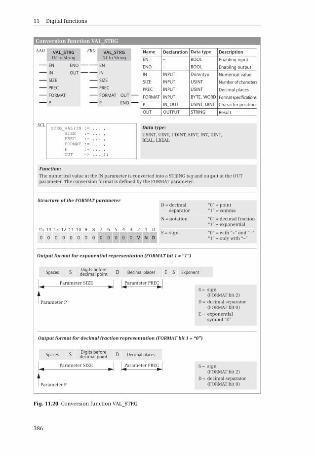
11 Digital functions
386
Fig. 11.20 Conversion function VAL_STRG
VAL_STRGDT to String
VAL_STRGDT to String
EN
SIZE
FORMAT
EN
SIZE
FORMAT
OUT
OUT
ENO
ENO
Conversion function VAL_STRG
LAD FBD
IN
PREC
P
IN
PREC
P
DeclarationName
EN
IN
ENO
SIZE
PREC
P
FORMAT
OUT
–
INPUT
–
INPUT
INPUT
IN_OUT
INPUT
OUTPUT
BOOL
Datentyp
BOOL
USINT
USINT
USINT, UINT
BYTE, WORD
STRING
DescriptionData type
Structure of the FORMAT parameter
Function:
The numerical value at the IN parameter is converted into a STRING tag and output at the OUT parameter. The conversion format is defined by the FORMAT parameter.
Data type:
USINT, UINT, UDINT, SINT, INT, DINT,REAL, LREAL
0
15
0
14
0
13
0
12
0
11
0
10
0
9
0
8
0
7
0
6
0
5
0
4
0
3
V
2
N
1
D
0
Output format for exponential representation (FORMAT bit 1 = “1”)
Output format for decimal fraction representation (FORMAT bit 1 = “0”)
SCLSTRG_VAL(IN := ... ,
SIZE := ... ,PREC := ... ,FORMAT := ... ,P := ... ,OUT => ... );
D = decimal separator
“0” = point“1” = comma
N = notation “0” = decimal fraction“1” = exponential
S = sign “0” = with “+” and “–”“1” = only with “–”
Enabling input
Numerical value
Enabling output
Number of characters
Decimal places
Character position
Format specifications
Result
E SS DSpacesDigits beforedecimal point Decimal places Exponent
Parameter SIZE
Parameter P
Parameter PREC
S DSpaces Digits beforedecimal point Decimal places
Parameter SIZE
Parameter P
Parameter PREC
S = sign (FORMAT bit 2)
D = decimal separator (FORMAT bit 0)
E = exponential symbol “E”
S = sign (FORMAT bit 2)
D = decimal separator (FORMAT bit 0)

11.6 Conversion functions (Conversion of data type)
387
Conversion of a number into a string (VAL_STRG)
The conversion function VAL_STRG converts a numerical value at the IN parameterinto a string and outputs it at the OUT parameter. OUT must be occupied by a validSTRING tag which is long enough to accommodate the converted value (Fig. 11.20).
The first converted character is written into the STRING tag at the position specifiedat the P parameter. If P is greater than the current length of the string, spaces areappended up to the P position. Following the conversion, the position of the nextcharacter in the string which has not yet been replaced is present in P.
The SIZE parameter specifies the number of digits in front of the decimal point.Leading spaces are inserted if the converted value occupies fewer digits.
The PREC parameter specifies the decimal places, even with a whole number. Exam-ple: The number 123 is converted on PREC = 1 into the string “12.3”. The maximumvalue for PREC is 7. If PREC = 0, the decimal separator and the decimal places can beomitted.
The floating point notation places an “E” before the exponent, followed by the signof the exponent and the exponent without leading zeros. The digits before the “E”are assigned as in fixed-point notation.
If an error occurs during processing of the conversion function, ENO is set to “0”.The OUT parameter then contains a value with leading spaces and with a “C” as thelast character.
11.6.8 Conversion functions STRG_TO_CHARS and CHARS_TO_STRG
The function STRG_TO_CHARS converts a string with data type STRING into anarray with data type ARRAY OF CHAR or ARRAY OF BYTE. The functionCHARS_TO_STRG converts an array with data type ARRAY OF CHAR or ARRAY OFBYTE into a string with data type STRING. In LAD and FBD, the conversion func-tions are displayed as EN/ENO boxes (Fig. 11.21).
STRG_TO_CHARS converts the string at the parameter STRG with data type STRINGinto a character sequence. The character sequence is inserted into the array at theparameter CHARS. The array comprises components with data type CHAR or BYTE.The position where the character sequence is inserted is specified by the parameterPCHARS. The parameter CNT indicates the number of inserted characters.
CHARS_TO_STRG converts a character sequence into a string with data type STRINGand outputs it at the parameter STRG. The character sequence is taken from thearray at the parameter CHARS. The parameter PCHARS specifies the position of thefirst character, while parameter CNT specifies the number of removed characters. Ifthe value is zero at parameter CNT, all characters are copied. The array has the datatype ARRAY OF CHAR or ARRAY OF BYTE. Only characters with ASCII coding areaccepted.
If an error occurs during conversion (e.g. if the target area is too small to accept thecopied characters), ENO is reset to signal state “0”.

11 Digital functions
388
Fig. 11.21 Conversion functions STRG_TO_CHARS and CHARS_TO_STRG
Conversion function STRG_TO_CHAR
Strg_TO_Chars Strg_TO_Chars
Chars_TO_Strg Chars_TO_Strg
EN EN
EN EN
pChars pChars
pChars pChars
Chars Chars
Cnt Cnt
Cnt
ENO
Strg
ENO
ENO
Cnt
ENO
Strg
LAD
LAD
FBD
FBD
Strg Strg
Chars Chars
Declaration
Declaration
Name
Name
EN
EN
Strg
Chars
ENO
ENO
pChars
pChars
Chars
Cnt
Cnt
Strg
–
–
INPUT
INPUT
–
–
INPUT
INPUT
INOUT
INPUT
OUTPUT
OUTPUT
BOOL
BOOL
BOOL
BOOL
DINT
DINT
STRING
VARIANT
VARIANT
UINT
UINT
STRING
Enabling input
Enabling input
String
Character array
Enabling output
Enabling output
Position
Position
Character array
Number
Number
String
Description
Description
Data type
Data type
Function:
Function:
SCL
SCL
Strg_TO_Chars(Strg := ... , pChars := ... , Cnt => ... , Chars := ... );
Chars_TO_Strg(Chars := ... , pChars := ... , Cnt := ... , Strg => ... );
current length
maximum length
Parameter pChars
Parameter pChars
Cnt
Cnt
Parameter Strg
Parameter Strg
Parameter Chars
Parameter Chars
The string at the STRG parameter is inserted from the position PCHARS in the character array at the CHARS parameter with the data type ARRAY OF CHAR or ARRAY OF BYTE. The CNT parameter indicates the number of inserted characters.
From the character array at the parameter CHARS with the data type ARRAY OF CHAR or ARRAY OF BYTE, CNT characters after the position PCHARS are taken, converted to a string, and output at the STRG parameter.
Conversion function CHARS_TO_STRG
Valid characters:
all characters with ASCII coding
current length
maximum length
11.7 Shift functions
389
11.6.9 Conversion functions ATH and HTA
The ATH function converts a sequence of ASCII-coded characters into a sequence ofhexadecimal numbers. The HTA function converts a sequence of hexadecimal num-bers into a sequence of ASCII-coded characters. The conversion functions are rep-resented as EN/ENO boxes in the case of LAD and FBD and as function calls with theconversion result as the function value in the case of SCL (Fig. 11.22).
Area pointers in the form of P#Data_block.Data_operand or P#Operand that point tothe first byte of the input or output data area are expected at the IN and OUT param-eters. Example: P#DB10.DBX12.0. The N parameter with data type INT specifies thenumber of characters to be converted.
ATH converts a character sequence present in ASCII code into a sequence in hexa-decimal code. Only the digits 0 to 9 and the uppercase letters A to F are permissible.An illegal character is converted to zeros. In the event of error at parameterRET_VAL, an error message is output and ENO is reset to signal state “0”.
HTA converts a character sequence present in hexadecimal code into an ASCII-coded character sequence. HTA does not report any errors.
11.7 Shift functions
11.7.1 Introduction
A shift function moves the contents of the tags at parameter IN by as many digits asparameter N specifies. The result is output at the OUT parameter (Fig. 11.23).
The shift function is executed if “1” is present at the enabling input (“current” flowsinto the EN input) or if EN is unused. ENO is then “1”. The shift is not carried out ifit has not been enabled (EN = “0”), and ENO is also “0”. A shift function does not re-port any errors.
11.7.2 Shift to right (SHR)
The SHR shift function shifts the contents of the tag present at the IN input bit bybit to the right by the number of positions specified by the shift number at the Ninput. The bit positions that become free through shifting are filled with the datatypes SINT, INT, and DINT with the signal state of the most significant bit. The mostsignificant bit contains for the data types SINT, INT and DINT the sign of the fixed-point number.
With a fixed-point number, shifting to the right corresponds to a division by a pow-er to base 2. The exponent is then the shift number. The result of such a division cor-responds to the rounded-off integer.
If the shift number = 0, the function is not executed, and the value at the IN param-eter is output at the OUT parameter; if it is larger than the data width of the tag, itis shifted by the available places.
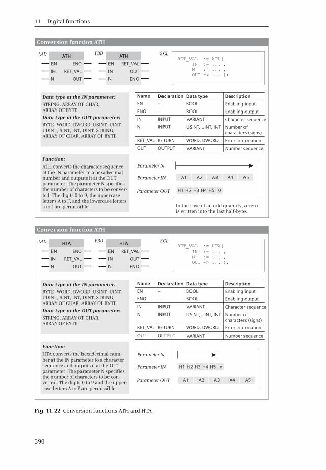
11 Digital functions
390
Fig. 11.22 Conversion functions ATH and HTA
Conversion function ATH
H1
H1
H2
H2
H3
H3
H4
H4
H5
H5
0
x
A1
A1
A2
A2
A3
A3
A4
A4
A5
A5
Parameter N
Parameter N
Parameter IN
Parameter IN
Parameter OUT
Parameter OUT
ATH
HTA
ATH
HTA
EN
EN
EN
EN
N
N
N
N
RET_VAL
RET_VAL
OUT
OUT
OUT
OUT
ENO
ENO
ENO
ENO
RET_VAL
RET_VAL
LAD
LAD
FBD
FBD
IN
IN
IN
IN
Declaration
Declaration
Name
Name
EN
EN
IN
IN
ENO
ENO
N
N
RET_VAL
RET_VAL
OUT
OUT
–
–
INPUT
INPUT
–
–
INPUT
INPUT
RETURN
RETURN
OUTPUT
OUTPUT
BOOL
BOOL
BOOL
BOOL
USINT, UINT, INT
USINT, UINT, INT
WORD, DWORD
WORD, DWORD
VARIANT
VARIANT
VARIANT
VARIANT
Character sequence
Number of characters (signs)
Error information
Number sequence
Character sequence
Number of characters (signs)
Error information
Number sequence
Description
Description
Data type
Data type
Function:
Function:
Data type at the OUT parameter:
STRING, ARRAY OF CHAR,ARRAY OF BYTE
BYTE, WORD, DWORD, USINT, UINT,UDINT, SINT, INT, DINT, STRING,ARRAY OF CHAR, ARRAY OF BYTE
BYTE, WORD, DWORD, USINT, UINT,UDINT, SINT, INT, DINT, STRING,ARRAY OF CHAR, ARRAY OF BYTE
STRING, ARRAY OF CHAR,ARRAY OF BYTE
SCL
SCL
RET_VAL := ATH(IN := ... ,N := ... ,OUT => ... );
RET_VAL := HTA(IN := ... ,N := ... ,OUT => ... );
Conversion function ATH
ATH converts the character sequence at the IN parameter to a hexadecimal number and outputs it at the OUT parameter. The parameter N specifies the number of characters to be conver-ted. The digits 0 to 9, the uppercase letters A to F, and the lowercase letters a to f are permissible. In the case of an odd quantity, a zero
is written into the last half-byte.
Data type at the IN parameter:
Data type at the IN parameter:
Data type at the OUT parameter:
Enabling input
Enabling output
Enabling input
Enabling output
HTA converts the hexadecimal num-ber at the IN parameter to a character sequence and outputs it at the OUT parameter. The parameter N specifies the number of characters to be con-verted. The digits 0 to 9 and the upper-case letters A to F are permissible.

11.7 Shift functions
391
11.7.3 Shift to left (SHL)
The shift function SHL shifts the contents of the tag at the IN input to the left,bit-y-bit, by the number of positions specified by the shift number at the N input.The bit positions which become vacant during shifting are padded with zeros.
With a fixed-point number, shifting to the left corresponds to a multiplication by apower to base 2. The exponent is then the shift number.
If the shift number = 0, the function is not executed, and the value at the IN param-eter is output at the OUT parameter; if it is larger than the data width of the tag, itis shifted by the available places.
11.7.4 Rotate to right (ROR)
The shift function ROR shifts the contents of the tag at the IN input to the right,bit-by-bit, by the number of places specified by the shift number at the N input.The bit positions which become vacant during shifting are padded with the bit po-sitions which have been shifted out.
If the shift number = 0, the function is not executed, and the value at the IN parameteris output at the OUT parameter; if it is larger than the data width of the tag, it is rotat-ed by the available places.
Fig. 11.23 Shift functions, representation and function
FunctionData type
FunctionData type
EN EN
OUT OUT
ENO
ENO
Shift functions
LAD FBD
IN
N N
IN
Function: SHRSHL
Shift to rightShift to left
Function: RORROL
Rotate to rightRotate to left
Data type: BYTE, WORD, DWORD,SINT, INT, DINT, USINT, UINT, UDINT
Data type: BYTE, WORD, DWORD
DeclarationName
EN
ENO
IN
N
OUT
–
–
INPUT
INPUT
OUTPUT
BOOL
BOOL
Data type
UINT
Data type
DescriptionData type
“0”
S
“0”
SHL
ROL
SHR
SHR
ROR
for SINT, INT, DINT:
for BYTE, WORD, DWORD, USINT, UINT, UDINT:
SCLOUT := (IN := ... , N := ... );Function
Enabling input
Enabling output
Input tag
Number
Result
11 Digital functions
392
11.7.5 Rotate to left (ROL)
The shift function ROL shifts the contents of the tag at the IN input to the left,bit-by-bit, by the number of places specified by the shift number at the N input.The bit positions which become vacant during shifting are padded with the bit po-sitions which have been shifted out.
If the shift number = 0, the function is not executed, and the value at the IN parameteris output at the OUT parameter; if it is larger than the data width of the tag, it is rotat-ed by the available places.
11.8 Logic functions
11.8.1 Introduction
The (digital) logic functions comprise the following functions:
b AND, OR, XORWord logic operations according to AND, OR, and XOR
b INVInvert
b DECO, ENCOCode bit and set bit number
b SEL, MUX, DEMUX, MIN, MAX, LIMITSelection functions, minimum and maximum selection, limiter
LAD and FBD: A logic function is performed if the enable input is “1” or if “current”is flowing into the EN input or if EN is not connected. ENO is then “1”. In the eventof error, ENO is “0”. If the execution of the function is not enabled (EN = “0”), pro-cessing does not take place and ENO is also “0”.
SCL: If the function execution is faulty, the tag ENO is set to FALSE.
11.8.2 Word logic operations (AND, OR, XOR)
The word logic operations link the values of two tags at the parameters IN1 and IN2according to AND, OR, or XOR. Depending on the data type, the logic operation isperformed byte by byte, word by word, or doubleword by doubleword. The result isoutput at the OUT parameter (Fig. 11.24).
The word logic operation generates the result bit by bit. Bit 0 of the IN1 input islinked to bit 0 of the IN2 input; the result is saved in bit 0 of the OUT output. Thesame logic operation takes place with bit 1, bit 2, etc.
AND operation
The AND logic operation links the individual bits of the value present at the IN1 in-put to the corresponding bits of the value at the IN2 input according to AND.

11.8 Logic functions
393
The individual bits in the result word OUT only have signal state “1” if the corre-sponding bits of both values to be linked have signal state “1”.
Since the bits with signal state “0” at the IN2 input also set these bits in the resultto “0”, independent of the assignments of these bits at the IN1 input, these bits arereferred to as being “masked”. This “masking” is the main field of application of the(digital) AND logic operation.
OR logic operation
The OR logic operation links the individual bits of the value present at the IN1 inputto the corresponding bits of the value at the IN2 input according to OR. The individ-ual bits in the result word OUT only have signal state “0” if the corresponding bitsof both values to be linked have signal state “0”.
Since the bits with signal state “1” at the IN2 input also set these bits in the resultto “1”, independent of the assignments of these bits at the IN1 input, these bits arereferred to as being “displayed”. This unmasking is the main field of application ofthe (digital) OR logic operation.
Exclusive OR operation
The exclusive OR logic operation links the individual bits of the value present at theIN1 input to the corresponding bits of the value at the IN2 input according toExclusive OR. The individual bits in the result word OUT only have signal state “1”if just one of the corresponding bits of the two values to be linked has signal state“1”. If a bit at the IN2 input has signal state “1”, this position in the result has theinverted signal state of the bit at the IN1 input. In the result, only those bits havesignal state “1” which have different signal states in the two tags prior to the digital
Fig. 11.24 Word logic operations, representation and function
EN EN
OUT OUT
ENO
ENO
LAD FBD
IN1
IN2 IN2
IN1
Function:ANDORXOR
AND Bit-by-bit AND operationBit-by-bit OR operationBit-by-bit exclusive OR operation
Data type:BYTE, WORD, DWORD
DeclarationName
EN
ENO
IN1
IN2
OUT
–
–
INPUT
INPUT
OUTPUT
BOOL
BOOL
Data type
Data type
Data type
DescriptionData type
Linking of individual bits:
Bit of parameter IN1Bit of parameter IN2
Result with ANDResult with ORResult with XOR
SCLOUT := IN1 IN2;Function
Enabling input
Enabling output
Input tag 1
Input tag 2
Result
“0” “0”“0” “0”
“0” “0” “0”“0”“0” “0”
“1” “1”“1”
“1”“1” “1” “1”“1” “1”
“1”
Digital logic operations AND, OR and XOR
FunctionData type
FunctionData type

11 Digital functions
394
Exclusive OR operation. The finding of the bits occupied by different signal statestogether with the negation of the signal states of individual bits is the main field ofapplication of the (digital) Exclusive OR logic operation.
11.8.3 Invert (INV)
The inversion negates the value at parameter IN bit by bit and writes it to the tag atparameter OUT. The bit-by-bit negation replaces the zeros with ones and vice versa.The function INV does not report any errors (Fig. 11.25).
11.8.4 Coding functions DECO and ENCO
The coding functions comprise the DECO functions (converting a binary numberinto a bit pattern) and ENCO (converting a bit pattern into a binary number). Fig.11.26 shows these functions.
Code bit DECO
DECO sets the bit whose number is at the IN parameter in the bit sequence tag atthe OUT parameter. All other bits are set to signal state “0”. Depending on the datatype at the OUT parameter, only some of the bits are selected in the IN parameter:3 bits (range 0 to 7) for BYTE, 4 bits (range 0 to 15) for WORD, and 5 bits (range 0 to31) for DWORD. The function DECO does not report any errors.
SCL: DECO returns the output parameter as function value. Its data type is DWORDby default. If the function value has a different data type, the data type is “attached”to the function name with an underscore. Example:
#var_byte := DECO_BYTE(#var_usint);
Fig. 11.25 Inverting, representation and function
INV INVData type Data type
EN EN
OUT
OUTENO
ENO
Invert
LAD FBD
IN IN
Function:
The inverted value of the tag at the IN parameter is output at the OUT parameter.
Data type:
BYTE, WORD, DWORD, USINT, UINT, UDINT, SINT, INT, DINT
DeclarationName
EN
ENO
IN
OUT
–
–
INPUT
OUTPUT
BOOL
BOOL
Datentyp
Datentyp
DescriptionData type
Linking of individual bits:
Bit of IN parameter
Bit of OUT parameter
SCL OUT := NOT IN;
Enabling input
Enabling output
Input tag
Result
“0”
“0”
“1”
“1“
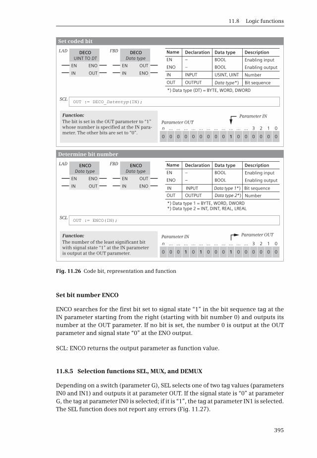
11.8 Logic functions
395
Set bit number ENCO
ENCO searches for the first bit set to signal state “1” in the bit sequence tag at theIN parameter starting from the right (starting with bit number 0) and outputs itsnumber at the OUT parameter. If no bit is set, the number 0 is output at the OUTparameter and signal state “0” at the ENO output.
SCL: ENCO returns the output parameter as function value.
11.8.5 Selection functions SEL, MUX, and DEMUX
Depending on a switch (parameter G), SEL selects one of two tag values (parametersIN0 and IN1) and outputs it at parameter OUT. If the signal state is “0” at parameterG, the tag at parameter IN0 is selected; if it is “1”, the tag at parameter IN1 is selected.The SEL function does not report any errors (Fig. 11.27).
Fig. 11.26 Code bit, representation and function
DECO
ENCO ENCO
DECO
EN
EN
EN
EN
OUT
OUT
OUT
OUT
ENO
ENO
ENO
ENO
Set coded bit
Determine bit number
LAD
LAD
FBD
FBD
IN
IN
IN
IN
Declaration
Declaration
Name
Name
EN
EN
ENO
ENO
IN
IN
OUT
OUT
–
–
–
–
INPUT
INPUT
OUTPUT
OUTPUT
BOOL
BOOL
BOOL
BOOL
USINT, UINT
Data type*)
Data type 1*)
Data type 2*)
Description
Description
Data type
Data type
UINT TO DT
Data type Data type
Data type
*)
*) Data type 1 = BYTE, WORD, DWORD*) Data type 2 = INT, DINT, REAL, LREAL
Parameter OUT
Parameter IN
Parameter IN
Parameter OUT
The bit is set in the OUT parameter to “1” whose number is specified at the IN para-meter. The other bits are set to “0”.
The number of the least significant bit with signal state “1” at the IN parameter is output at the OUT parameter.
Function:
Function:
0
0
n
n
0
0
...
...
0
0
...
...
0
1
...
...
0
0
...
...
0
1
...
...
0
0
...
...
0
0
...
...
0
0
...
...
1
1
...
...
0
0
...
...
0
0
...
...
0
0
3
3
0
0
2
2
0
0
1
1
0
0
0
0
SCL
SCL
OUT := DECO_ (IN);Datentyp
OUT := ENCO(IN);
Enabling input
Enabling output
Number
Bit sequence
Enabling input
Enabling output
Bit sequence
Number
Data type (DT) = BYTE, WORD, DWORD

11 Digital functions
396
Dependent on the value of the K parameter, MUX outputs a tags at the box inputs(parameters IN0 to INn and ELSE) at the OUT parameter. The MUX box is initiallyoffered by the program editor with a choice of two input values (IN0, IN1) and canthen be expanded to multiple values. MUX selects from these tag values (IN0 to INn)the one whose number is specified at parameter K. If K = 0, the tag at IN0 is selected;if K = 1, the tag at IN1, etc.
Fig. 11.27 Binary selection SEL, representation and function
Fig. 11.28 Multiplexing MUX, representation and function
EN EN
OUT
OUT
ENO
ENO
Binary selection SEL
LAD FBD
G
IN0
IN1
G
IN0
IN1
Data type:
USINT, UINT, UDINT, SINT, INT, DINT,REAL, LREAL,BYTE, WORD, DWORD, CHAR, TIME,
DeclarationName
EN
ENO
G
IN0
IN1
OUT
–
–
INPUT
INPUT
INPUT
OUTPUT
BOOL
BOOL
BOOL
Data type
Data type
Data type
DescriptionData type SEL SEL
Function:
SCL OUT := SEL(G := ... , IN0 := ... , IN1 := ...);
Enabling input
Enabling output
Switch
Input tag 0
Input tag 1
Result
Data type Data type
With signal state “0” at parameter G, the value at parameter IN0 is transferred to the parameter OUT, otherwise the value at parameter IN1.
EN EN
OUT
OUT
ENO
ENO
Multiple selection MUX
LAD FBD
K
IN0
IN1
ELSE ELSE
K
IN0
IN1
Data type :
USINT, UINT, UDINT, SINT, INT, DINT,REAL, LREAL,BYTE, WORD, DWORD, CHAR, TIME
DeclarationName
EN
ENO
K
IN1
IN0
ELSE
OUT
-
-
INPUT
INPUT
INPUT
INPUT
OUTPUT
BOOL
BOOL
UINT
Data type
Data type
Data type
Data type
Substitute value
Result
DescriptionData typeMUX MUX
Function:
SCL OUT := MUX(K := ... , IN1 := ... , IN2 := ... ,
* *
INELSE := ... );
Enabling input
Enabling output
Auswahl
Input tag 1
Input tag 0
Data type Data type
Depending on the assignment of parameter K, MUX transfers the value of an input parameter IN to the output parameter OUT. If the value at K is greater than the number of inputs, the value at the ELSE or INELSE parameter is transferred to the output.
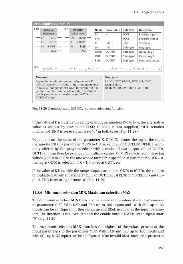
11.8 Logic functions
397
If the value of K is outside the range of input parameters IN0 to INn, the alternativevalue is output by parameter ELSE; if ELSE is not supplied, OUT remainsunchanged. ENO is set to signal state “0” in both cases (Fig. 11.28).
Dependent on the value of the parameter K, DEMUX issues the tag at the input(parameter IN) to a parameter OUT0 to OUTn, or ELSE or OUTELSE. DEMUX is ini-tially offered by the program editor with a choice of two output values (OUT0,OUT1) and can then be extended to multiple values. DEMUX selects from these tagvalues (OUT0 to OUTn) the one whose number is specified at parameter K. If K = 0,the tag at OUT0 is selected; if K = 1, the tag at OUT1, etc.
If the value of K is outside the range output parameters OUT0 to IOUTn, the value isoutput alternatively at parameter ELSE or OUTELSE ; if ELSE or OUTELSE is not sup-plied, ENO is set to signal state “0” (Fig. 11.29).
11.8.6 Minimum selection MIN, Maximum selection MAX
The minimum selection MIN transfers the lowest of the values at input parametersto parameter OUT. With LAD and FBD up to 100 inputs and with SCL up to 32inputs can be configured. If there is an invalid REAL number at the input parame-ters, the function is not executed and the enable output ENO is set to signal state“0” (Fig. 11.30).
The maximum selection MAX transfers the highest of the values present at theinput parameters to the parameter OUT. With LAD and FBD up to 100 inputs andwith SCL up to 32 inputs can be configured. If an invalid REAL number is present at
Fig. 11.29 Demultiplexing DEMUX, representation and function
EN EN
OUT0
OUT1
ELSE
ELSE
OUT1
OUT0ENO
ENO
Demultiplexing DEMUX
LAD FBD
K
IN
K
IN
Data type:
USINT, UINT, UDINT, SINT, INT, DINT,REAL, LREAL,BYTE, WORD, DWORD, CHAR, TIME
DeclarationName
EN
ENO
K
OUT0
IN
OUT1
ELSE
–
–
INPUT
OUTPUT
INPUT
OUTPUT
OUTPUT
BOOL
BOOL
UINT
Data type
Data type
Data type
Data type
DescriptionData typeDEMUX DEMUX
Function:
SCL DEMUX(K := ... , IN := ... , OUT1 => ... , OUT2 => ... , OUTELSE => ... );
**
Output tag 1
Substitute output
Enabling input
Enabling output
Selection
Output tag 0
Input tag
Data type Data type
Depending on the assignment of parameter K, DEMUX transfers the value of the input parameter IN to an output parameter OUT. If the value at K is greater than the number of outputs, the value at the IN parameter is transferred to the ELSE or OUTELSE output.

11 Digital functions
398
the input parameters, the function is not executed, and the enabling output ENO isset to signal state “0”.
11.8.7 Limiter LIMIT
The limiter LIMIT compares the value at parameter IN with the values of theparameters MIN and MAX. If the value at IN is between the limits, it is output atparameter OUT; it is less than MIN, the value is output at OUT; if it is above MAX,the value goes to MAX. The upper and lower limits can also be assigned constantvalues (Fig. 11.31).
If there is an invalid REAL number at the parameters MIN, IN, or MAX, an invalidREAL number is output and the enable output ENO is set to signal state “0”. Theenable output is also set to “0” if the value at parameter MIN is greater than thevalue at parameter MAX; the value is then output at parameter IN.
11.9 Processing of strings (Data type STRING)
A string can be processed using the following functions:
b LEN Outputs the length of a stringb CONCAT Combines two strings togetherb LEFT Outputs the left part of a stringb RIGHT Outputs the right part of a stringb MID Outputs the middle part of a stringb DELETE Deletes part of a stringb INSERT Inserts characters into a stringb REPLACE Replaces characters in a stringb FIND Outputs the position of a searched character
Fig. 11.30 Minimum and maximum selection, representation and function
EN EN
OUT
ENO
OUT
ENO
Minimum selection MIN, Maximum selection MAX
LAD FBD
IN1
IN2
IN1
IN2
Function:
MIN
MAX
Minimum selection
Maximum selection
Data type:
USINT, UINT, UDINT,SINT, INT, DINT,REAL, LREAL
DeclarationName
EN
ENO
IN1
IN2
OUT
–
–
INPUT
INPUT
OUTPUT
BOOL
BOOL
Data type
Data type
Data type
DescriptionData type
SCL OUT := (IN1 := ... , IN2 := ... );Function
* *
Enabling input
Enabling output
Input tag 1
Input tag 2
Result
FunctionData type
FunctionData type
The lowest input value is copied to the OUT output.
The highest input value is copied to the OUT output
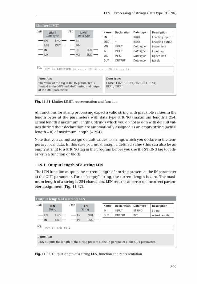
11.9 Processing of strings (Data type STRING)
399
All functions for string processing expect a valid string with plausible values in thelength bytes at the parameters with data type STRING (maximum length 254,actual length maximum length). Strings which you do not assign with default val-ues during their declaration are automatically assigned as an empty string (actuallength = 0) of maximum length (= 254).
Note that you cannot assign default values to strings which you declare in the tem-porary local data. In this case you must assign a defined value (this can also be anempty string) to a STRING tag in the program before you use the STRING tag togeth-er with a function or block.
11.9.1 Output length of a string LEN
The LEN function outputs the current length of a string present at the IN parameterat the OUT parameter. For an “empty” string, the current length is zero. The maxi-mum length of a string is 254 characters. LEN returns an error on incorrect param-eter assignment (Fig. 11.32).
Fig. 11.31 Limiter LIMIT, representation and function
Fig. 11.32 Output length of a string LEN, function and representation
EN EN
OUT
ENO
OUT
ENO
Limiter LIMIT
LAD FBD
MN
IN
MX
MN
IN
MX
Data type:
USINT, UINT, UDINT, SINT, INT, DINT,REAL, LREAL
Function:
DeclarationName
EN
ENO
MN
IN
MX
OUT
–
–
INPUT
INPUT
INPUT
OUTPUT
BOOL
BOOL
Data type
Data type
Data type
Data type
DescriptionData typeLIMITData type
LIMITData type
SCL OUT := LIMIT(MN := ... , IN := ... , MX := ... );
Enabling input
Enabling output
Lower limit
Input tag
Upper limit
Result
The value of the tag at the IN parameter is limited to the MIN and MAX limits, and output at the OUT parameter.
EN EN
OUT
ENO OUT
ENO
Output length of a string LEN
LAD FBD
IN IN
DeklarationName
IN
OUT
INPUT
OUTPUT
STRING
INT
String
Actual length
DescriptionData typeLENString
LENString
Function:
LEN outputs the length of the string present at the IN parameter at the OUT parameter.
SCL OUT := LEN(IN);
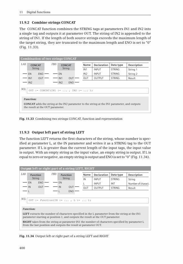
11 Digital functions
400
11.9.2 Combine strings CONCAT
The CONCAT function combines the STRING tags at parameters IN1 and IN2 intoa single tag and outputs it at parameter OUT. The string of IN2 is appended to thestring of IN1. If the length of both source strings exceeds the maximum length ofthe target string, they are truncated to the maximum length and ENO is set to “0”(Fig. 11.33).
11.9.3 Output left part of string LEFT
The function LEFT returns the first characters of the string, whose number is spec-ified at parameter L, at the IN parameter and writes it as a STRING tag to the OUTparameter. If L is greater than the current length of the input tags, the input valueis output. With an empty string as the input value, an empty string is output. If L isequal to zero or negative, an empty string is output and ENO is set to “0” (Fig. 11.34).
Fig. 11.33 Combining two strings CONCAT, function and representation
Fig. 11.34 Output left or right part of a string LEFT and RIGHT
EN EN
OUT
ENO
OUT
ENO
Combination of two strings CONCAT
LAD FBD
IN1
IN2
IN1
IN2
CONCAT CONCAT
Function:
DeclarationName
IN1
IN2
OUT
INPUT
INPUT
OUTPUT
STRING
STRING
STRING
DescriptionData type
SCL OUT := CONCAT(IN1 := ... , IN2 := ... );
String 1
String 2
Result
String String
CONCAT adds the string at the IN2 parameter to the string at the IN1 parameter, and outputs the result at the OUT parameter.
DeclarationName
IN
L
OUT
INPUT
INPUT
OUTPUT
STRING
INT
STRING
DescriptionData type
EN EN
OUT
ENO
OUT
ENO
Output left or right part of a string LEFT, RIGHTen
LAD FBD
IN
L
IN
L
Function:
SCL OUT := (IN := ... , L := ... );Function
String
Number of charact.
Result
Function FunctionString String
LEFT extracts the number of characters specified in the L parameter from the string at the IN1 parameter starting at position 1, and outputs the result at the OUT parameter.
RIGHT takes from the string at parameter IN1 the number of characters specified by parameter L from the last position and outputs the result at parameter OUT.

11.9 Processing of strings (Data type STRING)
401
11.9.4 Output right part of string RIGHT
The RIGHT function delivers the last characters (whose number is specified at theL parameter) from the string applied to the IN parameter, and writes them as aSTRING tag to the OUT parameter. If L is greater than the current length of the inputtags, the input value is output. An empty string is output if the input value is anempty string. If L is equal to zero or negative, an empty string is output and ENO isset to “0” (Fig. 11.34).
11.9.5 Output middle part of string MID
The MID function extracts a middle section of the string present at the IN parame-ter, and outputs it at the OUT parameter. The middle section starts at the positionspecified at the P parameter, and has as many characters as defined by the L param-eter (Fig. 11.35).
If the sum of P and L exceeds the current length of the input tags, a string beginningat position P and reaching to the end is output. If P is outside the current length ofIN, a blank string is output and ENO is set to “0”. If P or L is zero or negative, a blankstring is output and ENO is set to “0”.
11.9.6 Delete part of a string DELETE
The DELETE function removes part of the string at the IN parameter and outputs the“collapsed” remainder at the OUT parameter. The removed part begins at the char-acter position specified by parameter P and has as many characters as specified inparameter L (Fig. 11.36).
Fig. 11.35 Output the middle part of a string MID, function and representation
DeclarationName
IN
L
P
OUT
INPUT
INPUT
INPUT
OUTPUT
STRING
INT
INT
STRING
DescriptionData type
EN EN
OUT
ENO
OUT
ENO
Output middle section of a string MID
LAD FBD
IN
L
P
IN
L
P
MID MID
Function:
MID extracts the number of characters specified in the L parameter from the string at the IN1 parameter starting at position P, and outputs the result at the OUT parameter.
SCL OUT := MID(IN := ... , L := ... , P := ... );
Input tag
Number of charact.
Character position
Output tag
String String
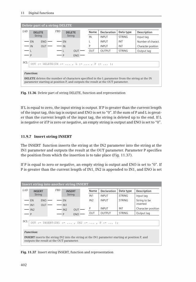
11 Digital functions
402
If L is equal to zero, the input string is output. If P is greater than the current lengthof the input tag, this tag is output and ENO is set to “0”. If the sum of P and L is great-er than the current length of the input tag, the string is deleted up to the end. If Lis negative or if P is zero or negative, an empty string is output and ENO is set to “0”.
11.9.7 Insert string INSERT
The INSERT function inserts the string at the IN2 parameter into the string at theIN1 parameter and outputs the result at the OUT parameter. Parameter P specifiesthe position from which the insertion is to take place (Fig. 11.37).
If P is equal to zero or negative, an empty string is output and ENO is set to “0”. IfP is greater than the current length of IN1, IN2 is appended to IN1, and ENO is set
Fig. 11.36 Delete part of string DELETE, function and representation
Fig. 11.37 Insert string INSERT, function and representation
DeclarationName
IN
L
P
OUT
INPUT
INPUT
INPUT
OUTPUT
STRING
INT
INT
STRING
DescriptionData type
EN EN
OUT
ENO
OUT
ENO
Delete part of a string DELETE
LAD FBD
IN
L
P
IN
L
P
DELETEString
DELETEString
Function:
DELETE deletes the number of characters specified in the L parameter from the string at the IN parameter starting at position P, and outputs the result at the OUT parameter.
SCL OUT := DELETE(IN := ... , L := ... , P := ... );
Input tag
Number of charact.
Character position
Output tag
DeclarationName
IN1
IN2
P
OUT
INPUT
INPUT
INPUT
OUTPUT
STRING
STRING
INT
STRING
DescriptionData type
EN EN
OUT
ENO
OUT
ENO
Insert string into another string INSERT
LAD FBD
IN1
IN2
P
IN1
IN2
P
INSERTString
INSERTString
Function:
INSERT inserts the string IN2 into the string at the IN1 parameter starting at position P, and outputs the result at the OUT parameter.
SCL OUT := INSERT(IN1 := ... , IN2 := ... , P := ... );
Input tag
String to be inserted
Character position
Output tag
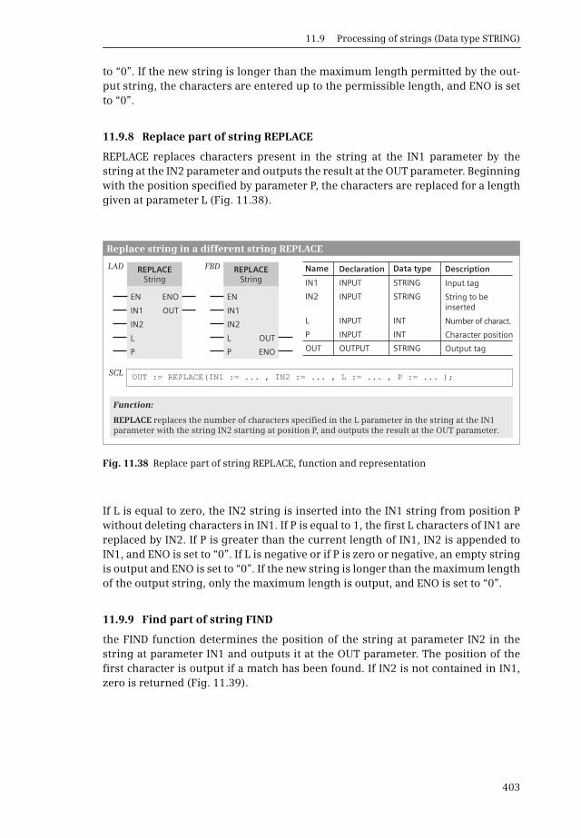
11.9 Processing of strings (Data type STRING)
403
to “0”. If the new string is longer than the maximum length permitted by the out-put string, the characters are entered up to the permissible length, and ENO is setto “0”.
11.9.8 Replace part of string REPLACE
REPLACE replaces characters present in the string at the IN1 parameter by thestring at the IN2 parameter and outputs the result at the OUT parameter. Beginningwith the position specified by parameter P, the characters are replaced for a lengthgiven at parameter L (Fig. 11.38).
If L is equal to zero, the IN2 string is inserted into the IN1 string from position Pwithout deleting characters in IN1. If P is equal to 1, the first L characters of IN1 arereplaced by IN2. If P is greater than the current length of IN1, IN2 is appended toIN1, and ENO is set to “0”. If L is negative or if P is zero or negative, an empty stringis output and ENO is set to “0”. If the new string is longer than the maximum lengthof the output string, only the maximum length is output, and ENO is set to “0”.
11.9.9 Find part of string FIND
the FIND function determines the position of the string at parameter IN2 in thestring at parameter IN1 and outputs it at the OUT parameter. The position of thefirst character is output if a match has been found. If IN2 is not contained in IN1,zero is returned (Fig. 11.39).
Fig. 11.38 Replace part of string REPLACE, function and representation
DeclarationName
IN1
IN2
L
P
OUT
INPUT
INPUT
INPUT
INPUT
OUTPUT
STRING
STRING
INT
INT
STRING
DescriptionData type
EN EN
OUT
ENO
OUT
ENO
Replace string in a different string REPLACE
LAD FBD
IN1
L
IN2
P
IN1
L
IN2
P
REPLACEString
REPLACEString
Function:
SCL OUT := REPLACE(IN1 := ... , IN2 := ... , L := ... , P := ... );
Input tag
String to be inserted
Number of charact.
Character position
Output tag
REPLACE replaces the number of characters specified in the L parameter in the string at the IN1 parameter with the string IN2 starting at position P, and outputs the result at the OUT parameter.

11 Digital functions
404
11.10 Calculating with the CALCULATE box in LAD and FBD
The CALCULATE box can link digital tags with arithmetic, mathematical, and logi-cal functions in a complex expression with each other. You define the tags to belinked as input parameters of the box and specify the data type of the expression(the output parameter). The logic operation function is specified in a dialog (Fig.11.40).
In the basic state, the box contains two inputs. The number of inputs can beincreased. The inputs are numbered without gaps. Not all inputs must be used inthe expression. If, when defining the expression, a (new) input with the next avail-able number is used, the input is automatically added. In the expression, only thetags defined as input parameters may be used.
After inserting the CALCULATE box, select the data type of the expression (the out-put parameter OUT) from a drop-down list. The input parameters will automati-cally be given the same data type. The actual operands must be of the same datatype or a data type that can be converted using implicit conversion to the data typeof the input parameter. Example: If you select data type LREAL for the expression,an actual operand with the data type REAL or LREAL can be created at an input.
In the expression, the input tags can be linked with each other according to theirdata type. The order of the linking can be controlled using brackets.
Linking of bit strings
Input parameters with the data types BYTE, WORD, and DWORD can be used in con-nection with the word logic operations AND (digital AND logic operation), OR (dig-ital OR logic operation), and XOR (digital exclusive OR logic operation). A bit stringcan be inverted with the NOT operator (one's complement formation INV). WithSWAP(), the bytes of a bit string can be replaced.
Fig. 11.39 Find part of string FIND, function and representation
EN EN
OUT
ENO
OUT
ENO
Find string in a different string FIND
LAD FBD
IN1
IN2
IN1
IN2
DeclarationName
IN1
IN2
OUT
INPUT
INPUT
OUTPUT
STRING
STRING
INT
DescriptionData typeFINDString
FINDString
Function:
FIND searches for string IN2 in the string at the IN1 parameter, and outputs its position at the OUT parameter.
SCL OUT := FIND(IN1 := ... , IN2 := ... );
Input tag
String to be found
Output tag
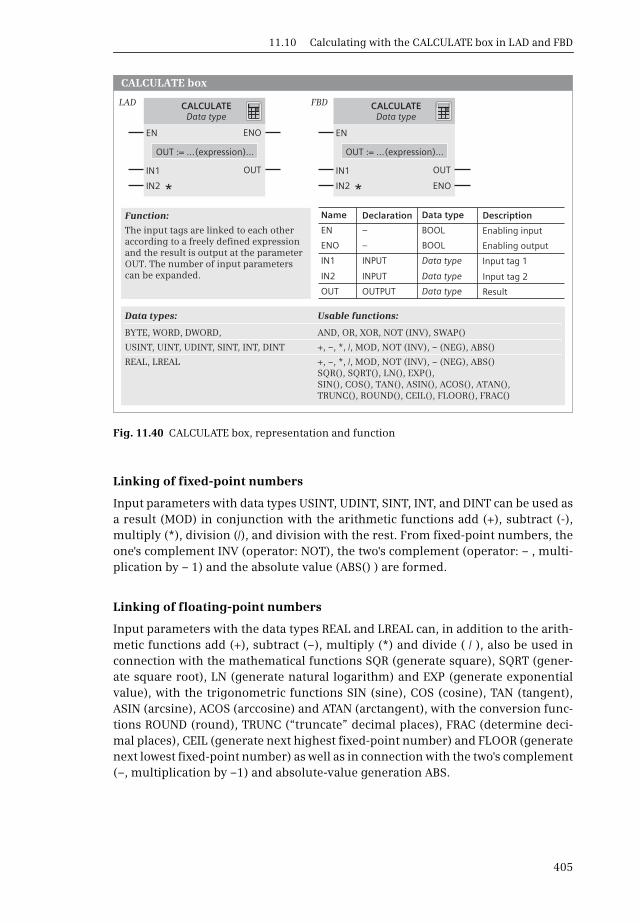
11.10 Calculating with the CALCULATE box in LAD and FBD
405
Linking of fixed-point numbers
Input parameters with data types USINT, UDINT, SINT, INT, and DINT can be used asa result (MOD) in conjunction with the arithmetic functions add (+), subtract (-),multiply (*), division (/), and division with the rest. From fixed-point numbers, theone's complement INV (operator: NOT), the two's complement (operator: – , multi-plication by – 1) and the absolute value (ABS() ) are formed.
Linking of floating-point numbers
Input parameters with the data types REAL and LREAL can, in addition to the arith-metic functions add (+), subtract (–), multiply (*) and divide ( / ), also be used inconnection with the mathematical functions SQR (generate square), SQRT (gener-ate square root), LN (generate natural logarithm) and EXP (generate exponentialvalue), with the trigonometric functions SIN (sine), COS (cosine), TAN (tangent),ASIN (arcsine), ACOS (arccosine) and ATAN (arctangent), with the conversion func-tions ROUND (round), TRUNC (“truncate” decimal places), FRAC (determine deci-mal places), CEIL (generate next highest fixed-point number) and FLOOR (generatenext lowest fixed-point number) as well as in connection with the two's complement(–, multiplication by –1) and absolute-value generation ABS.
Fig. 11.40 CALCULATE box, representation and function
DeclarationName
EN
ENO
IN1
IN2
OUT
–
–
INPUT
INPUT
OUTPUT
BOOL
BOOL
Data type
Data type
Data type
DescriptionData type
CALCULATEData type
CALCULATEData type
EN EN
IN1 IN1
IN2 IN2
ENO
ENO
OUT OUT
CALCULATE box
LAD FBD
Data types: Usable functions:
BYTE, WORD, DWORD, AND, OR, XOR, NOT (INV), SWAP()
USINT, UINT, UDINT, +, –, *, /, MOD, NOT (INV), – (NEG), ABS()
REAL, LREAL
SINT, INT, DINT
+, –, *, /, MOD, NOT (INV), – (NEG), ABS()SQR(), SQRT(), LN(), EXP(),SIN(), COS(), TAN(), ASIN(), ACOS(), ATAN(),TRUNC(), ROUND(), CEIL(), FLOOR(), FRAC()
Function:
* *
OUT := ...(expression)... OUT := ...(expression)...
The input tags are linked to each other according to a freely defined expression and the result is output at the parameter OUT. The number of input parameterscan be expanded.
Enabling input
Enabling output
Input tag 1
Input tag 2
Result
12 Program flow control
406
12 Program flow control
This chapter describes the functions for controlling program execution, indepen-dent of the programming language as far as possible. The Chapters 7 “Ladder logicLAD” on page 209, 8 “Function block diagram FBD” on page 246, and 9 “StructuredControl Language SCL” on page 284 describe how you can program the functionsusing the individual programming languages and what special features exist.
The jump functions allow program branches dependent upon or independently ofthe logic operation, a numerical value, or a comparison with a numerical value. Thecontrol statements which are only present with SCL for controlling program execu-tion are described in Chapter 9.6.3 “Control statements” on page 307.
The block functions are used to structure the user program. A block end functionprematurely terminates the processing in a block, the block call functions callanother block for processing. A block call is parameterizable and can be used mul-tiple times with different parameters. A block call can be controlled using theenable input EN and the enable output ENO.
12.1 Jump functions
12.1.1 Overview
Jump functions interrupt linear program execution in the block and continue at adifferent point in the program in the block. This point is identified by means of ajump label which you specify in the jump statement as the jump destination. Thejump function and destination must be in the same block. The jump destination orlabel must be unique within a block. It is permissible to jump to a destination frommore than one position. Both forward and backward jumps are possible with regardto the direction of program execution.
The following jump functions are available:
b Absolute jump, is always executed during processing.
b Conditional jump, is executed depending on the result of logic operation.
b Jump list, branches depending on a value
b Jump distributor, branches depending on a comparison result
Jump list and jump distributor are available in the described form for LAD and FBD.SCL uses control statements for program branches.

12.1 Jump functions
407
12.1.2 Absolute jump
An absolute jump is carried out independent of conditions. The absolute jumpinterrupts linear program execution and continues it at a the specified jump label.Fig. 12.1 shows the implementation of the jump function in the various program-ming languages.
Absolute jump function JMP (LAD and FBD)
The jump functions consist of the jump statement (coil or box) and a jump label.The jump label (jump destination) identifies the entry point in the block at whichprogram execution is continued when the jump function has been processed.
The jump function JMP is connected to the left-hand power rail or does not have apreceding logic operation. The entry point can only be positioned at the start of anetwork. Only one jump statement ore one block end function is permissible pernetwork.
Absolute jump GOTO (SCL)
The jump function GOTO interrupts the linear program execution and continues itat a different position in the block. If statements form a defined block, e.g. a pro-gram body within a program loop, the jump destination must be within this state-
Fig. 12.1 Absolute jump function JMP or GOTO
GOTO Destination ;... ;... ;
JMP
Destination
Destination
JMP
LAD
FBD
SCL
The absolute jump is executed independent of conditions during processing.
Destination
Destination
Absolute jump
If the JMP coil (jump with RLO = “1”) is connected to the left busbar, the jump function is always executed during processing.
The jump destination (jump label) is located at the beginning of the network in which the processing of the program is to be continued.
Destination: ... ;
If the input is not connected on the JMP box (jump with RLO = “1”), the jump function is always executed during processing.
The jump destination (jump label) is located at the beginning of the network in which the processing of the program is to be continued.
The GOTO statement is always executed during processing.
The jump destination (jump label) is located at the beginning of the program line in which processing is to be continued."

12 Program flow control
408
ment block if the GOTO statement is also within the statement block, and it cannotjump to this statement block “from the outside”.
A jump label must always be followed by a statement. A “dummy statement” is alsopermissible:
Label: ; //Entry with “dummy statement”
12.1.3 Conditional jump
A conditional jump is executed depending on the result of logic operation (RLO).Program execution is continued at the specified jump label with RLO = “1” or withRLO = “0” depending on the jump function. Fig. 12.2 shows the implementation ofthe conditional jump function in the various programming languages.
Fig. 12.2 Conditional jump functions JMP and JMPN
JMP
JMPN
Destination
Destination
Destination
Destination
JMP
JMPN
LAD
FBD
SCL
The conditional jump is executed depending on the result of logic operation (RLO).
(VKE)
(VKE)
(RLO)
(RLO)
Destination
Destination
IF (*RLO*) THEN GOTO Destination; END_IF;IF NOT (*RLO*) THEN GOTO Destination; END_IF;... ;... ;Destination: ... ;
Conditional jump
The JMP jump function is executed if RLO = “1” during processing. RLO = “0” has no effect.
The JMPN jump function is executed if RLO = “0” during processing. RLO = “1” has no effect.
The jump destination (jump label) is located at the beginning of the network in which the processing of the program is to be continued.
The JMP jump function is executed if RLO = “1” during processing. RLO = “0” has no effect."
The JMPN jump function is executed if RLO = “0” during processing. RLO = “1” has no effect."
The jump destination (jump label) is located at the beginning of the network in which the processing of the program is to be continued.
A jump that depends on the result of logic operation can be programmed with the IF statement.
The jump destination (the jump label) is located at the beginning of the program line in which processing is to be continued.
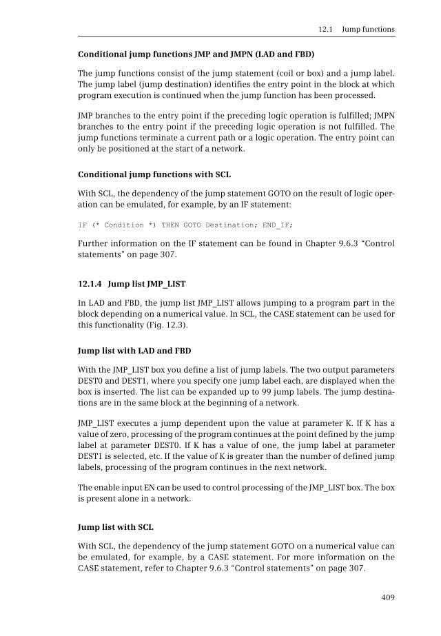
12.1 Jump functions
409
Conditional jump functions JMP and JMPN (LAD and FBD)
The jump functions consist of the jump statement (coil or box) and a jump label.The jump label (jump destination) identifies the entry point in the block at whichprogram execution is continued when the jump function has been processed.
JMP branches to the entry point if the preceding logic operation is fulfilled; JMPNbranches to the entry point if the preceding logic operation is not fulfilled. Thejump functions terminate a current path or a logic operation. The entry point canonly be positioned at the start of a network.
Conditional jump functions with SCL
With SCL, the dependency of the jump statement GOTO on the result of logic oper-ation can be emulated, for example, by an IF statement:
IF (* Condition *) THEN GOTO Destination; END_IF;
Further information on the IF statement can be found in Chapter 9.6.3 “Controlstatements” on page 307.
12.1.4 Jump list JMP_LIST
In LAD and FBD, the jump list JMP_LIST allows jumping to a program part in theblock depending on a numerical value. In SCL, the CASE statement can be used forthis functionality (Fig. 12.3).
Jump list with LAD and FBD
With the JMP_LIST box you define a list of jump labels. The two output parametersDEST0 and DEST1, where you specify one jump label each, are displayed when thebox is inserted. The list can be expanded up to 99 jump labels. The jump destina-tions are in the same block at the beginning of a network.
JMP_LIST executes a jump dependent upon the value at parameter K. If K has avalue of zero, processing of the program continues at the point defined by the jumplabel at parameter DEST0. If K has a value of one, the jump label at parameterDEST1 is selected, etc. If the value of K is greater than the number of defined jumplabels, processing of the program continues in the next network.
The enable input EN can be used to control processing of the JMP_LIST box. The boxis present alone in a network.
Jump list with SCL
With SCL, the dependency of the jump statement GOTO on a numerical value canbe emulated, for example, by a CASE statement. For more information on theCASE statement, refer to Chapter 9.6.3 “Control statements” on page 307.
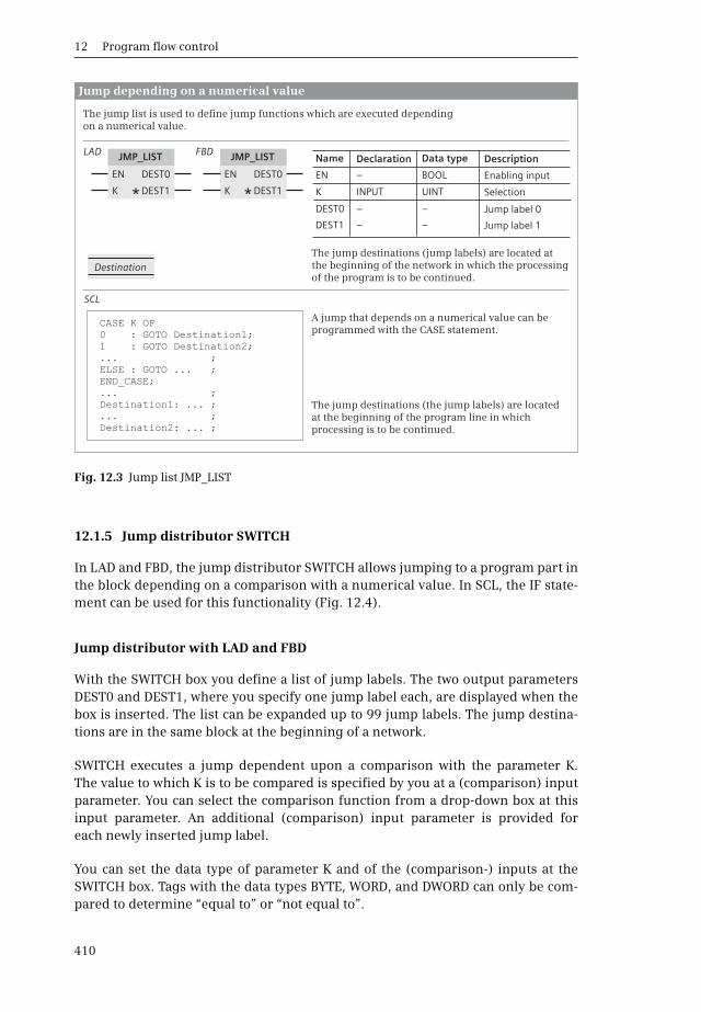
12 Program flow control
410
12.1.5 Jump distributor SWITCH
In LAD and FBD, the jump distributor SWITCH allows jumping to a program part inthe block depending on a comparison with a numerical value. In SCL, the IF state-ment can be used for this functionality (Fig. 12.4).
Jump distributor with LAD and FBD
With the SWITCH box you define a list of jump labels. The two output parametersDEST0 and DEST1, where you specify one jump label each, are displayed when thebox is inserted. The list can be expanded up to 99 jump labels. The jump destina-tions are in the same block at the beginning of a network.
SWITCH executes a jump dependent upon a comparison with the parameter K.The value to which K is to be compared is specified by you at a (comparison) inputparameter. You can select the comparison function from a drop-down box at thisinput parameter. An additional (comparison) input parameter is provided foreach newly inserted jump label.
You can set the data type of parameter K and of the (comparison-) inputs at theSWITCH box. Tags with the data types BYTE, WORD, and DWORD can only be com-pared to determine “equal to” or “not equal to”.
Fig. 12.3 Jump list JMP_LIST
Jump depending on a numerical value
LAD FBD
SCL
Destination
CASE K OF0 : GOTO Destination1;1 : GOTO Destination2;... ;ELSE : GOTO ... ;END_CASE;... ;Destination1: ... ;... ;Destination2: ... ;
EN ENDEST0 DEST0
DEST1 DEST1K K
DeclarationName
EN
K
DEST1
DEST0
–
INPUT
–
–
BOOL
UINT
–
–
Enabling input
Selection
Jump label 1
Jump label 0
DescriptionData typeJMP_LIST JMP_LIST
* *
The jump list is used to define jump functions which are executed depending on a numerical value.
The jump destinations (jump labels) are located at the beginning of the network in which the processing of the program is to be continued.
A jump that depends on a numerical value can be programmed with the CASE statement.
The jump destinations (the jump labels) are located at the beginning of the program line in which processing is to be continued.
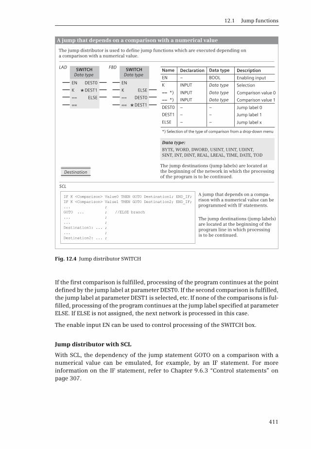
12.1 Jump functions
411
If the first comparison is fulfilled, processing of the program continues at the pointdefined by the jump label at parameter DEST0. If the second comparison is fulfilled,the jump label at parameter DEST1 is selected, etc. If none of the comparisons is ful-filled, processing of the program continues at the jump label specified at parameterELSE. If ELSE is not assigned, the next network is processed in this case.
The enable input EN can be used to control processing of the SWITCH box.
Jump distributor with SCL
With SCL, the dependency of the jump statement GOTO on a comparison with anumerical value can be emulated, for example, by an IF statement. For moreinformation on the IF statement, refer to Chapter 9.6.3 “Control statements” onpage 307.
Fig. 12.4 Jump distributor SWITCH
A jump that depends on a comparison with a numerical value
LAD FBD
SCL
Data type:
BYTE, WORD, DWORD, USINT, UINT, UDINT,SINT, INT, DINT, REAL, LREAL, TIME, DATE, TOD
Destination
IF K <Comparison> Value0 THEN GOTO Destination1; END_IF;
... ;GOTO ... ; //ELSE branch... ;... ;Destination1: ... ;... ;Destination2: ... ;
IF K <Comparison> Value1 THEN GOTO Destination2; END_IF;
EN ENDEST0
DEST0
DEST1
DEST1
ELSE
ELSEK K
== ==
== ==
DeclarationName
EN
K
== *)
DEST1
== *)
DEST0
ELSE
*) Selection of the type of comparison from a drop-down menu
–
INPUT
INPUT
–
INPUT
–
–
BOOL
Data type
Data type
–
Data type
–
–
Enabling input
Selection
Comparison value 1
Jump label 1
Comparison value 0
Jump label 0
Jump label x
DescriptionData typeSWITCHData type
SWITCHData type
*
*
The jump distributor is used to define jump functions which are executed depending on a comparison with a numerical value.
The jump destinations (jump labels) are located at the beginning of the network in which the processing of the program is to be continued.
A jump that depends on a compa-rison with a numerical value can be programmed with IF statements.
The jump destinations (jump labels) are located at the beginning of the program line in which processing is to be continued.

12 Program flow control
412
12.2 Block end function
You can use the block end function RET or RETURN to prematurely terminate pro-cessing in a block (Fig. 12.5).
Block end with LAD and FBD
The block end function is programmed as a RET coil or RET box at the end of a net-work. If the preceding logic operation has been completed, the block is left (condi-tional block end). A return is made to the previously processed block in which theblock call was present. If an organization block is terminated, a branch is made tothe operating system. If the preceding logic operation has not been completed, thenext network in the block is processed.
If the RET coil is connected to the left-hand power rail or if the RLO is fixed at “1” atthe box input or is unused, the block is always left (absolute block end). A subse-quent network can then only be processed if it has a jump label and is accessed bya jump function.
In the return tags, a signal state can be saved, which is mapped to the ENO output atthe call box (see Chapter 12.4 “EN/ENO mechanism” on page 417). To set the returntags, double-click on the RET function and select Ret from the drop-down box (RLO,corresponds to the result of logic operation), Ret True or Ret False for a constantvalue, or Ret Value for a tag. If an organization block ends with the block end func-tion, the signal state of the return tags has no meaning.
In a network with a jump function JMP or JMPN, there can be no Block end function.The block end function can be programmed multiple times in a block. The blockend function is not needed to end a block. It does not need to be programmed at theend of a block.
Fig. 12.5 Block end function RET or RETURN
Block end function
RET
RET
LAD
FBD
SCL
Function:
ENO := ... ;RETURN;.........IF <Condition> THEN RETURN;END_IF;
Exiting the block dependent upon the result of logic operation can be programmed with an IF statement.
If the RETURN statement is processed, the block is exited. The value of the ENO tag is transferred to the enable output ENO when the block is exited.
Return tag
Return tag
If the RET coil or box with signal state “1” is processed, the block is left. The signal state of the return tag is mapped when leaving the block in the enabling output ENO of the call box.

12.3 Calling of code blocks
413
Block end with SCL
With RETURN the currently processed block is exited without conditions. A condi-tional block end can be programmed using the IF statement. If an organizationblock is terminated, processing is continued in the CPU's operating system.
RETURN transfers the signal state of the ENO tag to the enable output of the exitedblock. If an organization block is exited via RETURN, the signal state of ENO has nomeaning. Programming of RETURN at the end of the block is optional.
12.3 Calling of code blocks
12.3.1 Introduction
If a logic block is to be edited, it must be “called up”. With LAD and FBD, the blockcall consists of the call box which contains the name (symbolic address) of the calledblock, the enable input EN, the enable output ENO, and the parameter list. WithSCL, the block name is specified during the block call, followed by the parameterlist. The enable input EN and the enable output ENO can be inserted into the param-eter list of a function block call.
Following processing of the call function, the CPU continues program execution inthe called block. The block is processed up to a block end function or up to its end.The CPU then returns to the calling block and continues processing of this blockafter the call function.
An organization block cannot be called; it is started by the operating systemdepending on events. If an organization block is terminated, the CPU continues towork in the operating system.
You can pass data on to the called block for processing, or accept data from thecalled block. The data is transferred by the block parameters.
You can use the enable input EN to structure the block call depending on the resultof logic operation. The called block can report faulty processing to the calling blockvia the enable output ENO. Further details can be found in Chapter 12.4 “EN/ENOmechanism” on page 417. The block properties, the design of the block interface,and the transfer of block parameters are described in Chapters 5.3 “Programmingblocks” on page 125 and 5.4 “Calling blocks” on page 137.
12.3.2 Calling a function FC
Calling a function (FC) is depicted in LAD and FBD with the call box. In SCL, it isdepicted with the block name and the parameter list (Fig. 12.6).
The prerequisite for calling a function (FC) is that the function must already be inthe user program. You program the call by dragging the block from the projecttree under Program blocks to the opened block. To call a function located in a
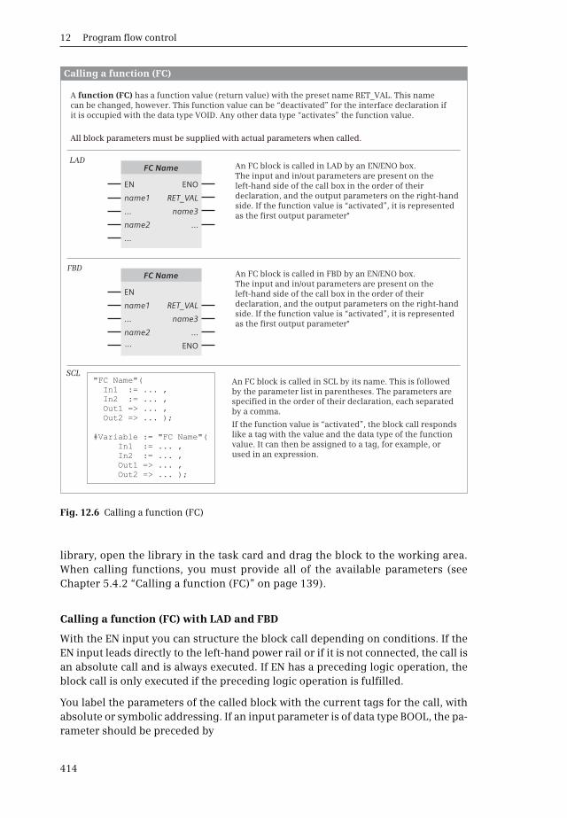
12 Program flow control
414
library, open the library in the task card and drag the block to the working area.When calling functions, you must provide all of the available parameters (seeChapter 5.4.2 “Calling a function (FC)” on page 139).
Calling a function (FC) with LAD and FBD
With the EN input you can structure the block call depending on conditions. If theEN input leads directly to the left-hand power rail or if it is not connected, the call isan absolute call and is always executed. If EN has a preceding logic operation, theblock call is only executed if the preceding logic operation is fulfilled.
You label the parameters of the called block with the current tags for the call, withabsolute or symbolic addressing. If an input parameter is of data type BOOL, the pa-rameter should be preceded by
Fig. 12.6 Calling a function (FC)
FC Name
FC Name
EN
EN
name1
name1
...
...
name2
name2
...
...
RET_VAL
name3
RET_VAL
name3
...
...
ENO
ENO
Calling a function (FC)
LAD
FBD
SCL" "FC Name (
In1 := ... ,In2 := ... ,Out1 => ... ,Out2 => ... );
#Variable := FC Name (In1 := ... ,In2 := ... ,Out1 => ... ,Out2 => ... );
" "
A function (FC) has a function value (return value) with the preset name RET_VAL. This name can be changed, however. This function value can be “deactivated” for the interface declaration if it is occupied with the data type VOID. Any other data type “activates” the function value.
All block parameters must be supplied with actual parameters when called.
An FC block is called in LAD by an EN/ENO box. The input and in/out parameters are present on the left-hand side of the call box in the order of their declaration, and the output parameters on the right-hand side. If the function value is “activated”, it is represented as the first output parameter"
An FC block is called in SCL by its name. This is followed by the parameter list in parentheses. The parameters are specified in the order of their declaration, each separated by a comma.
If the function value is “activated”, the block call responds like a tag with the value and the data type of the function value. It can then be assigned to a tag, for example, or used in an expression.
An FC block is called in FBD by an EN/ENO box. The input and in/out parameters are present on the left-hand side of the call box in the order of their declaration, and the output parameters on the right-hand side. If the function value is “activated”, it is represented as the first output parameter"

12.3 Calling of code blocks
415
b A contact or a current path (LAD) or
b A binary tag or binary logic operation (FBD).
A Boolean output parameter cannot be connected further.
The calling of functions with a function value is identical to the calling of functionswithout a function value. The function value (with the declaration RETURN and adata type not equal to VOID) is depicted as the first output parameter.
Calling a function (FC) with SCL
You call a function (FC) without a function value with your name. This is followedby the parameter list in round brackets. You must assign values to all block param-eters; the sequence is defined by the declaration.
The call of a function (FC) with function value must be handled in the SCL programlike a tag which has the data type of the function value. The call function is thenpresent in the assignment or expression instead of the function value. The call func-tion is comprised of the block name, followed by the parameter list in parentheses.
With a function (FC) you cannot use the implicitly defined enable input EN. You canprogram an FC call depending on a condition without a function value using the IFstatement. If you wish to use the implicitly defined enable output ENO, add it to theparameter list as the last parameter.
12.3.3 Calling a function block (FB)
Calling a function block (FB) is depicted in LAD and FBD with the call box. In SCL, itis depicted with the instance name and the parameter list (Fig. 12.7).
The prerequisite for calling a function block is that the function block mustalready be in the user program. You program the call by dragging the block in theproject tree from the Program blocks folder to the opened block. To call a functionblock located in a library, open the library in the task card and drag the block tothe working area. Select the type of call in the following dialog.
In the Call options dialog, click on the Single instance button if the data of the func-tion block is to be saved in a separate data block (in the instance data block). If youcall an additional function block in a function block, you can save the data of thecalled function block in the instance data block of the calling function block. In thiscase, select the Multi-instance button in the Call options dialog.
When calling a function block you only have to supply the block parameters that aresaved as pointers. The block parameters that are not supplied retain their currentvalue (see Chapter 5.4.3 “Calling a function block (FB)” on page 140).
Calling a function block with LAD and FBD
With the EN input you can structure the block call depending on conditions. If theEN input leads directly to the left-hand power rail or if it is not connected, the call is
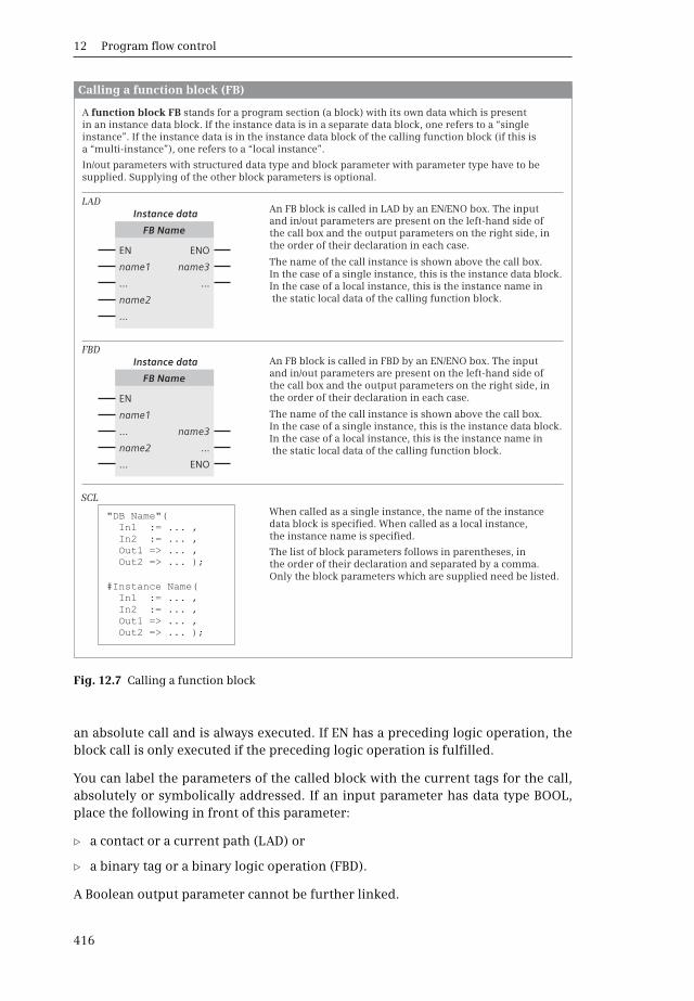
12 Program flow control
416
an absolute call and is always executed. If EN has a preceding logic operation, theblock call is only executed if the preceding logic operation is fulfilled.
You can label the parameters of the called block with the current tags for the call,absolutely or symbolically addressed. If an input parameter has data type BOOL,place the following in front of this parameter:
b a contact or a current path (LAD) or
b a binary tag or a binary logic operation (FBD).
A Boolean output parameter cannot be further linked.
Fig. 12.7 Calling a function block
Calling a function block (FB)
Instance data
Instance data
EN
EN
name1
name1
...
...
name2
name2
...
...
name3
name3
...
...
ENO
ENO
LAD
FBD
SCL
"DB Name"(In1 := ... ,In2 := ... ,Out1 => ... ,Out2 => ... );
#Instance Name(In1 := ... ,In2 := ... ,Out1 => ... ,Out2 => ... );
FB Name
FB Name
When called as a single instance, the name of the instancedata block is specified. When called as a local instance, the instance name is specified.
The list of block parameters follows in parentheses, in the order of their declaration and separated by a comma. Only the block parameters which are supplied need be listed.
The name of the call instance is shown above the call box. In the case of a single instance, this is the instance data block. In the case of a local instance, this is the instance name in the static local data of the calling function block.
An FB block is called in LAD by an EN/ENO box. The input and in/out parameters are present on the left-hand side of the call box and the output parameters on the right side, in the order of their declaration in each case.
An FB block is called in FBD by an EN/ENO box. The input and in/out parameters are present on the left-hand side of the call box and the output parameters on the right side, in the order of their declaration in each case.
The name of the call instance is shown above the call box. In the case of a single instance, this is the instance data block. In the case of a local instance, this is the instance name in the static local data of the calling function block.
A function block FB stands for a program section (a block) with its own data which is present in an instance data block. If the instance data is in a separate data block, one refers to a “single instance”. If the instance data is in the instance data block of the calling function block (if this is a “multi-instance”), one refers to a “local instance”.
In/out parameters with structured data type and block parameter with parameter type have to be supplied. Supplying of the other block parameters is optional.
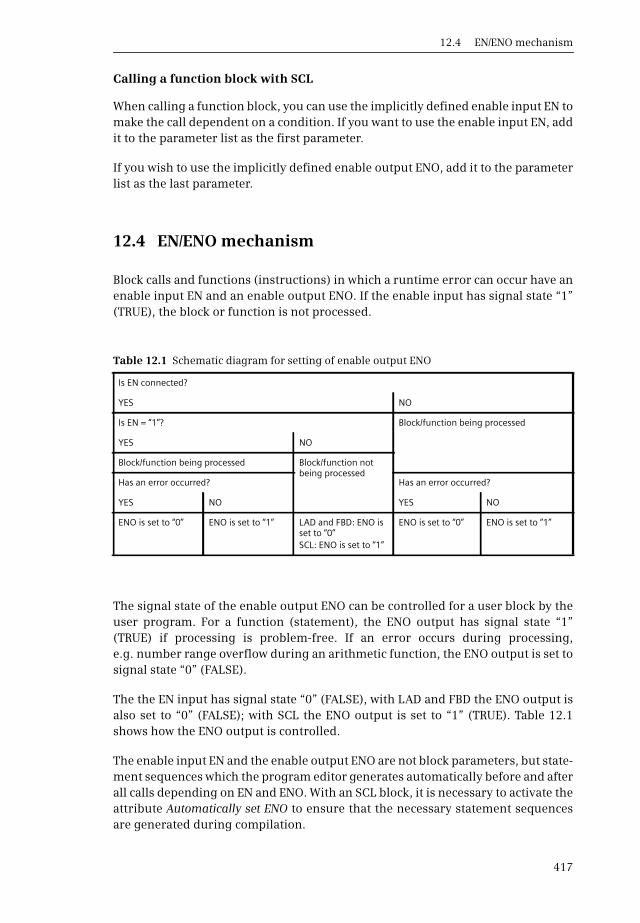
12.4 EN/ENO mechanism
417
Calling a function block with SCL
When calling a function block, you can use the implicitly defined enable input EN tomake the call dependent on a condition. If you want to use the enable input EN, addit to the parameter list as the first parameter.
If you wish to use the implicitly defined enable output ENO, add it to the parameterlist as the last parameter.
12.4 EN/ENO mechanism
Block calls and functions (instructions) in which a runtime error can occur have anenable input EN and an enable output ENO. If the enable input has signal state “1”(TRUE), the block or function is not processed.
The signal state of the enable output ENO can be controlled for a user block by theuser program. For a function (statement), the ENO output has signal state “1”(TRUE) if processing is problem-free. If an error occurs during processing,e.g. number range overflow during an arithmetic function, the ENO output is set tosignal state “0” (FALSE).
The the EN input has signal state “0” (FALSE), with LAD and FBD the ENO output isalso set to “0” (FALSE); with SCL the ENO output is set to “1” (TRUE). Table 12.1shows how the ENO output is controlled.
The enable input EN and the enable output ENO are not block parameters, but state-ment sequences which the program editor generates automatically before and afterall calls depending on EN and ENO. With an SCL block, it is necessary to activate theattribute Automatically set ENO to ensure that the necessary statement sequencesare generated during compilation.
Table 12.1 Schematic diagram for setting of enable output ENO
Is EN connected?
YES NO
Is EN = “1”? Block/function being processed
YES NO
Block/function being processed Block/function not being processed
Has an error occurred? Has an error occurred?
YES NO YES NO
ENO is set to “0” ENO is set to “1” LAD and FBD: ENO is set to “0”SCL: ENO is set to “1”
ENO is set to “0” ENO is set to “1”

12 Program flow control
418
Functions with an EN/ENO mechanism in the Statements folder in the program ele-ments catalog are the mathematical functions, moves, converters, digital logicoperations, move and rotate, all functions in the Expanded statements folder andall block calls.
12.4.1 EN/ENO mechanism with LAD and FBD
A contact or a binary tag or a preceding logic operation upstream of the enableinput EN controls the calling of the EN/ENO box. If the enable input EN is connectedto the left busbar or remains unconnected, the EN/ENO box is always processed.
You can use the properties of EN and ENO to connect several boxes into a sequence,where the enable output ENO leads to the enable input EN of the next box(Fig. 12.8). Thus, for example, the entire sequence can then be “deactivated” (nobox is processed, if the binary tag “Enable” in the example has signal state “0”) orthe rest of the sequence is no longer processed if a box reports an error.
12.4.2 EN/ENO mechanism with SCL
In SCL, the enable input EN and the enable output ENO are not included in the tem-plate of the function call or block call during programming. If you want to use theenable input EN when calling a function block, add it to the parameter list as thefirst parameter. If you would like to use the enable output ENO during a block call,insert it as the last parameter in the parameter list. Example of calling a functionblock as local instance:
#Instance_data(EN := #Enable, IN1 := ... , IN2 := ... , OUT => ... , ENO => #Error);If an error has occurred during block processing in the example, the tag #Error isset to FALSE; otherwise, it is set to TRUE. If the tag #Enable has the value FALSE inthe example, the block call is not carried out. The tag #Error is set to TRUE in thiscase.
Fig. 12.8 Series connection of ENO and EN

12.4 EN/ENO mechanism
419
12.4.3 EN/ENO for user blocks
Controlling the ENO output in LAD and FBD
With the block end function RET, you can influence the signal state of the enableoutput ENO: The release output ENO takes over the signal state of the return tag. If,for example, you want to set the enable output ENO to signal state “0” due to anerror found in the program, exit the block with RET and FALSE as the return value.
An example for this can be found in the Chapters 7.6 “Functions for program flowcontrol (LAD)” on page 241 and 8.6 “Functions for program flow control (FBD)” onpage 279.
Controlling the ENO output in SCL
When the block is exited, the enable output ENO assumes the value of the block-local tags ENO. A prerequisite is the activated attribute Automatically set ENO. ENOhas the value TRUE at the start of the block. An erroneously carried out statement,a numerical range overflow in an arithmetic function, for example, sets ENO toFALSE. If the block is now exited, the enable output ENO assumes the value FALSE.
The use of the block-local tags ENO is described in detail in Chapter 9.6.1 “Workingwith the ENO tag” on page 305.

13 Online operation, diagnostics and debugging
420
13 Online operation, diagnostics and debugging
One refers to online operation or online mode if a programming device is con-nected to a PLC or HMI station and an online connection has been established. Anonline connection is required in order to upload the user program to the CPU, totest it in the CPU during runtime, or to find hardware faults using diagnostic func-tions.
The connection between a programming device and a PLC station is made overIndustrial Ethernet. The mechanical connection (networking) and the logical con-nection (definition of the transmission protocols) are not configured. Only the net-work addresses – the addresses of the PROFINET interfaces of the two devices –must be matched to each other.
In online mode, STEP 7 Basic changes the display of the user interface: the title barsof the windows are displayed in orange. In the project tree, the objects of the sta-tions which are connected online are assigned symbols which indicate their operat-ing or diagnostics state.
You can use the online and diagnostics tools, for example, to control the operatingmode of the CPU, to set the time on the CPU, and fetch the diagnostic information,e.g. read the diagnostics buffer. The online and diagnostics tools support you introubleshooting during commissioning.
The user program which you have created offline can be transferred to the CPU inonline mode. When carried out for the first time, all configuration data and thecomplete user program are transferred, subsequently only the modified configura-tion data and program blocks. The transfer is always possible in the STOP operatingmode of the CPU. If certain prerequisites are met, it can also take place in the RUNoperating mode.
You can compare the online and offline versions of a block. Modifications to a blockare always carried out in the offline version which you then transfer to the CPU inthe STOP mode.
Two functions are available for testing the user program: the program status andthe watch tables. You use the program status to monitor the program executiondirectly on the control functions. The watch tables contain tags whose values youcan read and modify (control) during runtime or also set permanently (force).
The program editor also allows you to display the user program in a CPU without acorresponding offline project being present. If you then wish to edit the blocks, youmust first upload the online project into the offline data management.

13.1 Connecting a programming device to the PLC station
421
13.1 Connecting a programming device to the PLC station
The programming device can only exchange data with a PLC station if it isaddressed in the same subnet and has a node address which is different from thatof the PLC station. The IP addresses of the programming device and PLC stationmust therefore be identical in the part whose bits are occupied by “1” in the subnetmask, and different in the remaining part. You can find information on the struc-ture of the IP address and the subnet mask in Section “IP address and subnet mask”on page 73.
If the programming device already has an address different from that of the PLCstation, STEP 7 Basic sets a “temporary” IP address on the programming device.This temporary IP address is deleted again when Windows is shut down.
13.1.1 IP addresses of the programming device
Determining and setting network addresses using Windows tools
You can edit the network addresses of the programming device using the Networkconnections tool (Windows XP) or Network and enable center (Windows 7) in theWindows Control Panel. Open the Control Panel – for example from the Windowsdesktop via Start > Control Panel – and start the tool. Then double-click to select theLAN or WLAN connection that is used.
In the displayed status window Status of …, click on the Details button located in theGeneral or Network support tab. The currently active IP address and the subnetmask are displayed, for example. SIMATIC S7 supports the Internet protocol Version4 with the 4-byte long IPv4 address.
The connection status is displayed in the General tab. Click here on the Propertiesbutton. In the Properties of … window, select the Internet Protocol (TCP/IP) entry inthe This connection uses the following items field, and then click on the Propertiesbutton (Fig. 13.1).
In the following dialog Internet Protocol (TCP/IP) Properties you can set the IP ad-dress and subnet mask by selecting the Use the following IP address: option.
If you want to enter an additional IP address, for example for the SIMATIC project,click on the Advanced button. In the advanced settings, enter an additional IPaddress and the subnet mask in the IP Settings tab after clicking on the Add button.
Setting of access point
When installing STEP 7 Basic, the Set PG/PC interface tool is created in the WindowsControl Panel. This allows the user to check the access point to the Ethernet net-work and to reset it if necessary.
Open the Set PG/PC interface tool, for example from the Windows desktop using Start> Control Panel. The Access path tab should show S7ONLINE (STEP 7) in the Access

13 Online operation, diagnostics and debugging
422
point of application box. Select the LAN or WLAN interface module used under Inter-face Parameter Assignment Used and close the tool.
Determining IP addresses with STEP 7 Basic
If you wish to find out the IP address of the programming device (to be more pre-cise: the IP address of the interface module used) or, for example, wish to delete thetemporary IP address, proceed as follows:
Connect the interface module of the programming device to Ethernet, for exampleto a CPU. Switch on the CPU to activate the interface. The CPU can be in any operatingmode.
Start STEP 7 and change to the Project view. The virtual and physical online inter-faces of the programming device are listed in the project tree under Online access.Select the interface used and then the Properties command from the shortcutmenu. The MAC address, the fixed IP address, and the subnet mask are displayedin the properties dialog in the Configuration section under Industrial Ethernet. Allproject-specific IP addresses are listed under IE-PG access. You can delete all ofthese addresses using the Delete project-specific IP addresses button.
13.1.2 Connecting the programming device to the PLC station
Connect the LAN connection of the programming device to the PROFINET interfaceof the CPU module. You can use a standard or crossover cable since the CPU moduleis suitable for both types. Make sure that no memory card is inserted in theCPU module, and then switch on the power supply to the CPU module.
Fig. 13.1 Setting IP addresses with the Windows Control Panel
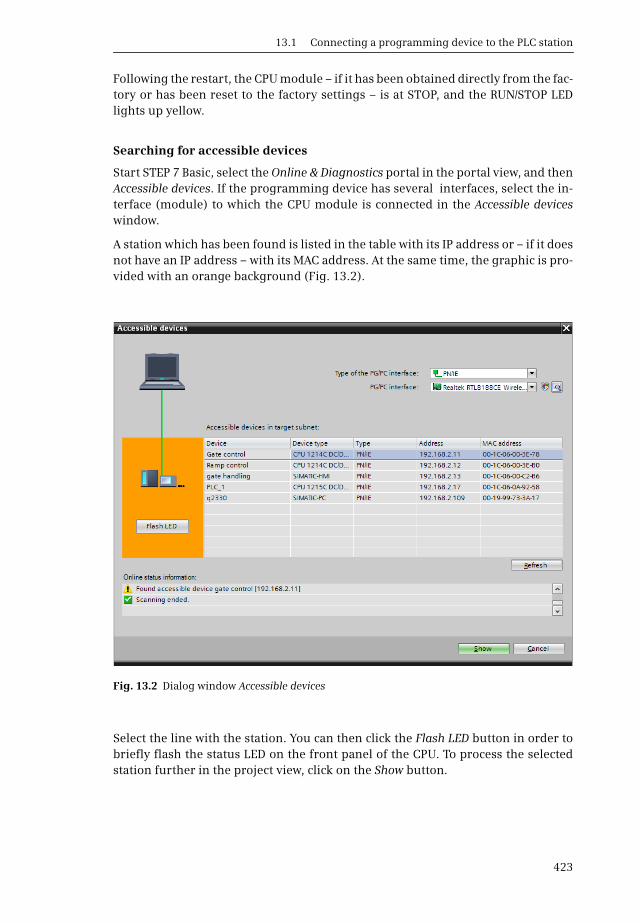
13.1 Connecting a programming device to the PLC station
423
Following the restart, the CPU module – if it has been obtained directly from the fac-tory or has been reset to the factory settings – is at STOP, and the RUN/STOP LEDlights up yellow.
Searching for accessible devices
Start STEP 7 Basic, select the Online & Diagnostics portal in the portal view, and thenAccessible devices. If the programming device has several interfaces, select the in-terface (module) to which the CPU module is connected in the Accessible deviceswindow.
A station which has been found is listed in the table with its IP address or – if it doesnot have an IP address – with its MAC address. At the same time, the graphic is pro-vided with an orange background (Fig. 13.2).
Select the line with the station. You can then click the Flash LED button in order tobriefly flash the status LED on the front panel of the CPU. To process the selectedstation further in the project view, click on the Show button.
Fig. 13.2 Dialog window Accessible devices

13 Online operation, diagnostics and debugging
424
Setting a temporary IP address on the programming device
If the network settings of the programming device do not agree with those of theCPU module, STEP 7 Basic allows you to set an appropriate, project-specific IP ad-dress on the programming device. This IP address is only present temporarily untilyou switch off the programming device or delete the address. Answer the corre-sponding dialogs with Yes or OK in order to assign an IP address. The assignedIP address is displayed in the response dialog.
STEP 7 Basic now shows the found CPU in the project view, and this is positionedwith its IP or MAC address in the Online access group under the used interface mod-ule as a new group in the project tree.
13.1.3 Assigning an IP address to the CPU module
If a CPU module is displayed with its MAC address, you can assign an IP address toit: select the PLC station and then the Online & Diagnostics command from theshortcut menu. Select the Assign IP address entry in the diagnostics window in theFunctions section. Enter the desired IP address and subnet mask, and click on theAssign IP address button. The result of the action is signaled in the Inspectorwindow in the Info tab.
13.1.4 Switching on the online mode
If you select the PLC station present under Online access in the project tree and thenOnline & Diagnostics from the shortcut menu, the online tools are displayed withthe CPU operator panel and the diagnostics window. Further details can be foundin Section 13.3 “Hardware diagnostics” on page 436.
If the project matching the online PLC station is present, open it and select thePLC station in the project tree. Select Go online from the shortcut menu, or activatethe Go online symbol in the main menu. The status of the PLC station is displayedin the Inspector window in the Diagnostics tab. Diagnostics symbols in the projecttree signal agreement between the online and offline versions of the blocks andPLC tags (see Section 13.3.6 “Further diagnostics information via the programmingdevice” on page 440).
Alternatively you can switch to online mode by selecting the Online & Diagnosticscommand in the shortcut menu with the PLC station selected. The diagnostics win-dow is then opened. Now click on the Go online button in the Online access section.
Further procedure
b How you can use the diagnostics and online tools, for example in order to startand stop the CPU or to reset to the default settings, can be found in Section 13.3“Hardware diagnostics” on page 436.
b The following Chapter 13.2 “Transferring project data” describes how you canupload a user program to the PLC station and edit the user program online.

13.2 Transferring project data
425
b Chapter 13.4 “Testing the user program” on page 441 describes how you can testa user program.
b Chapter 13.2.7 “Editing online project without offline project” on page 433 de-scribes how you can access the online project data of the CPU without the userprogram.
13.2 Transferring project data
You have configured the hardware and completed and compiled the user program.Downloading to the PLC station can be carried out in the following ways:
b Transfer via an online connection
b Transfer using a memory card as a transfer card
b Transfer using a memory card as a program card
The project data can only be downloaded when the CPU is in the STOP mode.
13.2.1 Loading project data for the first time
A CPU module without project data – for example if it has been obtained directlyfrom the factory – is in the STOP mode following connection of the power supply.In order to download the project data, connect the programming device to theCPU module, switch it on, and open the project.
Select the PLC station in the project tree and then the Download to the device > Allcommand from the shortcut menu. When loading for the first time, the dialog win-dow Advanced loading shows the IP address of the PLC station in the Configuredaccess nodes of … table. If the programming device has several interface modules,select the interface at which the PLC station is connected from the PG/PC interfacedrop-down list.
The PLC station does not have an IP address, or a different one
If the configured IP address does not agree with the IP address set in the CPU, STEP7 cannot find the device matching the configuration. This is indicated by an errormessage in the Extended download to device dialog window. In this window, activatethe Show all accessible devices check box. Browsing is then started again.
The found devices with their IP address are displayed in the Accessible devices intarget subnet table. The MAC address is displayed if a device does not have anIP address. Select the desired PLC station in this table, and click on the Load button.
If the network settings of the programming device do not match the configured IPaddress, the dialog window Assign IP address is displayed. STEP 7 then inquireswhether the programming device is to be assigned a further temporary, project-specific IP address. Acknowledge the inquiry with Yes or with OK.
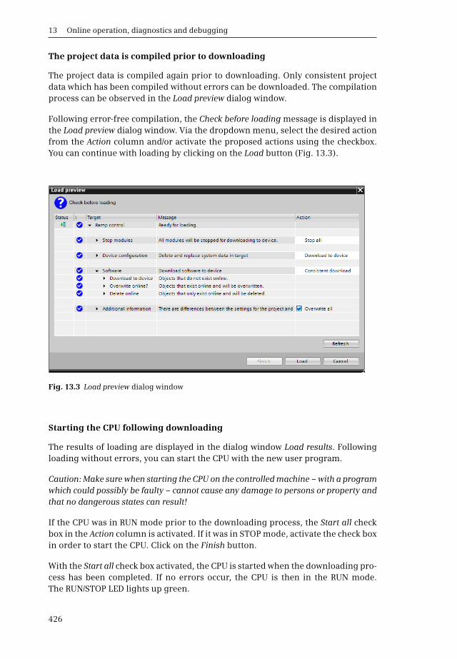
13 Online operation, diagnostics and debugging
426
The project data is compiled prior to downloading
The project data is compiled again prior to downloading. Only consistent projectdata which has been compiled without errors can be downloaded. The compilationprocess can be observed in the Load preview dialog window.
Following error-free compilation, the Check before loading message is displayed inthe Load preview dialog window. Via the dropdown menu, select the desired actionfrom the Action column and/or activate the proposed actions using the checkbox.You can continue with loading by clicking on the Load button (Fig. 13.3).
Starting the CPU following downloading
The results of loading are displayed in the dialog window Load results. Followingloading without errors, you can start the CPU with the new user program.
Caution: Make sure when starting the CPU on the controlled machine – with a programwhich could possibly be faulty – cannot cause any damage to persons or property andthat no dangerous states can result!
If the CPU was in RUN mode prior to the downloading process, the Start all checkbox in the Action column is activated. If it was in STOP mode, activate the check boxin order to start the CPU. Click on the Finish button.
With the Start all check box activated, the CPU is started when the downloading pro-cess has been completed. If no errors occur, the CPU is then in the RUN mode.The RUN/STOP LED lights up green.
Fig. 13.3 Load preview dialog window

13.2 Transferring project data
427
Switching on and testing online operation
Following loading of the project data, you can activate online mode by means of theGo online symbol in the main menu. The title bar of the active window has an orangebackground. You can open the diagnostics window using the Online & Diagnosticscommand from the shortcut menu of the selected PLC station. You can then use theonline tools, for example the CPU operator panel.
If you open a block in the project tree, you can use the Monitoring on/off symbol inthe toolbar of the working window to switch on the program status and to debugthe program. The possibilities offered by STEP 7 for program debugging are de-scribed in Section 13.4 “Testing the user program” on page 441.
13.2.2 Delta downloading of project data
When reloading project data, only the changes compared to the online project dataare loaded. It is possible to specify for the software (in the user program) whetheronly the changes are loaded or everything.
You determine with the download command which project data is to be download-ed. Select the object to be downloaded in the project tree and then the Download todevice > … command from the shortcut menu. You can:
b Select the All, Hardware configuration, Software or Software (all blocks) commands for the selected PLC station
b Select the Software or Software (all blocks) commands for the selected Program blocks folder
b Select the Software command for one or more selected blocks
The result of loading is shown in the inspector window under Info > General.
The CPU is in RUN mode
The configuration data can only be download in the STOP mode. If you select Down-load to device > … from the shortcut menu, you will be asked whether the selectedPLC station is to be set to STOP. Loading is canceled using Cancel, the CPU is set toSTOP using OK, and the loading process is continued with the compilation of theproject data.
The project data is partially up-to-date
If only the configuration data has been modified, for example, the Load preview dia-log window shows following compilation of the project data that the unmodifiedproject data is not loaded, e.g. The software is not downloaded because the online sta-tus is up-to-date. Select the desired actions and continue loading by clicking on theLoad button.

13 Online operation, diagnostics and debugging
428
Starting the CPU
If the CPU was in RUN mode prior to the downloading process, the Load results dia-log window then inquires whether the CPU is to be started (Start modules afterdownloading to device message with Start all check box activated).
Caution: Make sure when starting the CPU on the controlled machine – with a programwhich could possibly be faulty – cannot cause any damage to persons or property andthat no dangerous states can result!
Continue by clicking on the Finish button. The downloading process has been com-pleted when the RUN/STOP LED lights up permanently following short flashing.
Downloading a non-consistent program following faulty compilation
If an error is detected when compiling prior to downloading, this is signaled in theLoad preview dialog window. The component at which the error has occurred is in-dicated in the Target column under Compile (click the triangle on the left of this).It is only possible to continue the downloading process when the error has beeneliminated.
13.2.3 Error message following downloading
If the CPU does not start following loading – the RUN/STOP LED remains yellow – orif the ERROR LED flashes, the diagnostics buffer can provide information on thecause. Remaining in the STOP mode or returning to it could be the result of, forexample, a faulty I/O access in the user program. If the CPU is in RUN and the ERRORLED is flashing, there may be a difference between configured and actual hardware,for example.
Section 13.3.3 “Diagnostics buffer” on page 437 describes how the diagnostics buf-fer can support you during troubleshooting.
13.2.4 Working with the memory card
A SIMATIC Memory Card for a CPU 1200 is an SD memory card (secure digital mem-ory card) preformatted by Siemens. If you wish to delete the contents of the mem-ory card, you must only delete files or folders. Formatting the memory card makesit unusable in a CPU 1200. Please make sure that the write protection – the smallslide switch on the side of the card – is switched off if it is used in the CPU.
If you insert or remove a memory card when the CPU is in the RUN mode, the modeimmediately changes to STOP. Caution: Make sure that stopping of the CPU cannotcause any damage to persons or property and that no dangerous states can result!
Setting the type of card
You can use the memory card as a transfer card or as a program card. You can usethe transfer card as a replacement for the online connection to download a projectto the CPU; the program card replaces the internal load memory.

13.2 Transferring project data
429
To set the type of card, insert the memory card into the programming device's cardreader. In the project tree, open the SIMATIC Card Reader folder and the subordinatefolders down to the SD card (to the drive letter). Select the SD card and click on theProperties command in the shortcut menu. In the dialog window that is then dis-played, select the Program or Transfer entry from the drop-down list in the Card typefield.
Transferring project data to the memory card
Once the memory card has been set as a transfer or program card, copy the projectdata of the PLC station onto the memory card, e.g. using Copy with the PLC stationselected and Insert from the shortcut menu with the SD subsequently selected, orby dragging the PLC station to the memory card with the mouse button pressed.The project will be compiled. Following error-free compilation, the Load previewwindow is displayed; continue the downloading process with the Continue checkbox activated by clicking on the Load button. Click the Complete button to termi-nate the downloading process.
Using the memory card as a transfer card
Insert the memory card into the CPU module. If the CPU was in the RUN mode, itchanges to STOP. The MAINT LED flashes as an indication that the memory card hasto be evaluated. The memory card is evaluated following a CPU restart, e.g. whenswitching the power supply off and on again.
Following the restart, the project data is transferred from the memory card to theinternal load memory. The flashing MAINT LED signals the end of the transfer.You must remove the memory card before starting the CPU again.
You can start the CPU by switching the power supply off and on again, for example.The CPU starts with the set operating mode.
If the memory card is an empty transfer card, the internal load memory of the CPUis deleted during the transfer. A password-protected user program can be deletedin this manner if the password is unknown.
Using the memory card as a program card
Insert the memory card into the CPU module. If the CPU was in the RUN mode, itchanges to STOP. The MAINT LED flashes as an indication that the memory card hasto be evaluated. The memory card is evaluated following a CPU restart, e.g. whenswitching the power supply off and on again.
The contents of the internal load memory are deleted following the CPU restart, andthe executable data transferred from the memory card to the work memory.The CPU has the set operating mode following the restart.
The memory card must remain in the CPU module since it now contains the loadmemory. If the memory card is removed during runtime, the CPU goes to STOP andthe ERROR LED flashes.

13 Online operation, diagnostics and debugging
430
If the memory card is an empty program card, the contents of the internal loadmemory of the CPU are transferred to the memory card following a CPU restart. Fol-lowing a further CPU restart, the memory card is then used as an external loadmemory.
Fig. 13.4 Use of the memory card as transfer and program card
Project data is present on the transfer card.
Project data is present on the program card.
The transfer card is empty.
The program card is empty.
Use as transfer card
Use as program card
The project data is transferred to the memory card.
The project data is transferred to the memory card.
The data on the memory card is deleted.
The data on the memory card is deleted.
The memory card is inserted into the CPU. When switching on, the CPU imports the data into the internal load memory. The memory card can then be removed.
The memory card is inserted into the CPU. When switching on, the CPU replaces the internal load memory by the memory card. The memory card must remain inserted.
The memory card is inserted into the CPU. When switching on, the CPU deletes the data in the internal load memory (application: a password-protected program is to be deleted).
The memory card is inserted into the CPU. When switching on, the CPU copies the data from the internal load memory into the memory card. The memory card must remain inserted (as load memory).
Use of the memory card
S
S
S
S
CPU 1200
CPU 1200
CPU 1200
CPU 1200
s s
s s
ss
s s
13.2 Transferring project data
431
13.2.5 Processing blocks offline/online
Prerequisites: you have transferred the project data from the programming deviceto the CPU, the project is open, and the CPU connected online.
The program editor displays the user interface either in offline or online mode.In offline mode, the project data in the programming device is displayed; in onlinemode, the data in the CPU. You can swap between the two modes using the Go onlineand Go offline symbols in the toolbar of the project view. How to switch to onlinemode for the first time is described in Section 13.1 “Connecting a programming de-vice to the PLC station” on page 421.
Changing the CPU's configuration data
It is only possible to change the configuration data in offline mode. Switch to offlinemode, change the configuration data offline, and transfer it to the CPU. If you wishto transfer only the configuration data, select the PLC station in the project tree andthen the Download to device > Hardware configuration command from the shortcutmenu. The CPU is switched to STOP during downloading.
Changing a block in the CPU
It is only possible to change program blocks in offline mode. If you wish to changethe program of a block in the CPU during program debugging, you must switch tooffline mode, change the block in the offline data management, and then transferit to the CPU. The switch to online mode again and continue with debugging.
Online mode is switched on; the title bar of the active window has an orange back-ground, the title bars of the inactive windows are underlined in orange. Blockswhich are the same offline and online are identified by a green filled circle in theproject tree. A block is open, and you wish to change this block's program.
If you wish to carry out the changes on the online version of the block, the color ofthe title bar of the working window is changed, i.e. the program editor has automat-ically switched to the offline block which you can then change. A circle divided intwo colors in the project tree indicates that there is a difference between the offlineand online versions of the block.
Following completion of the change, transfer the modified block to the CPU: selectthe block and then the Download to device > Software command from the shortcutmenu. Follow the displayed dialog windows. The CPU must be set to STOP duringthe downloading process, and subsequently restarted.
Adding a block online
You can generate a new block in the offline data management using the Add newblock tool in the project tree, even if online mode is switched on. Program the blockoffline, and program the block call as well – if the new block is not an organizationblock – and then transfer both blocks to the CPU.

13 Online operation, diagnostics and debugging
432
Deleting a block online
You delete a block by selecting it and then the Delete command from the shortcutmenu. If the online mode is switched on and you wish to delete a block which ispresent both online and offline, the program editor inquires which of the blocks isto be deleted: the online block (Delete from device), the offline block (Delete fromproject), or both.
Before deleting a block in the CPU, you should delete its call, i.e. remove the call ofthe block to be deleted from the calling online block, otherwise the error The calledblock does not exist is signaled during runtime.
13.2.6 Comparing blocks offline/online
The compare editor enables you to compare the offline and online versions ofblocks. The comparison is possible in the STOP and RUN modes.
To start the compare editor, select the object to be compared in the project tree,e.g. the PLC station, the Program blocks folder, or individual blocks. Select the Com-pare > Offline/online command from the shortcut menu, or the command Tools >Compare > Offline/online in the main menu.
The comparison editor displays the compared objects and the comparison status inthe working window. As standard, objects which have different offline and onlineversions are displayed (Fig. 13.5). The filter icon in the toolbar can be used to switchto a display of all objects. In addition, the compared objects are also identified by acomparison symbol in the project tree.
A green filled circle indicates that the offline and online versions are identical.A blue/orange circle indicates that the object is different in the offline and onlineversions. If one half circle is not filled, the corresponding version is missing (leftside or blue represents offline, right side or orange represents online). An excla-mation mark in an orange circle indicates an object with differences in the namedfolder.
Fig. 13.5 Example of an offline/online comparison with different objects

13.2 Transferring project data
433
In the Action column, you can select the desired action from a dropdown menu,such as Download to device, if the offline version differs from the online version.Clicking on the Execute actions icon in the toolbar starts the set actions.
You can start a detailed comparison - providing the object allows it - if you select anobject with different versions and select Start detailed comparison, either in theshortcut menu or via the icon. In a successful detailed comparison, both versionsare opened at the point with the first difference and the detected difference is visi-ble in the inspection window in the Comparison result tab (Fig. 13.6).
Following elimination of the differences and execution of the appropriate down-loading action, you can start the comparison editor again using the Refresh the viewsymbol.
Note that only one offline/offline comparison or one offline/online comparison canbe carried out at a time.
13.2.7 Editing online project without offline project
You can access the project data in a CPU using the programming device even with-out offline project data.
Connect the programming device to the CPU, switch on the module and select theportal Online & Diagnostics and then Accessible nodes in the portal view. Set thePG/PC interface module if applicable. In the Accessible devices in target subnet list,select the PLC station and click on the Show button. If the programming device doesnot possess the matching network parameters, a dialog window is displayed toallow you to set these temporarily. Acknowledge with YES or OK.
Fig. 13.6 Example of a detailed comparison
13 Online operation, diagnostics and debugging
434
In the project view, the PLC station is displayed in the project tree of the interfacemodule used in the Online accesses folder. Select the PLC station and then theOnline & diagnostics editor from the shortcut menu. In online mode, you can selectthe mode using the CPU operator panel, for example, or read out the diagnosticsbuffer in the diagnostic functions.
The online blocks are present in the Program blocks folder. When you open the fold-er, STEP 7 downloads the blocks into it. A block is opened by double-clicking, andthe program in the block is displayed.
If you wish to edit or debug an online block, you must create an offline project andtransfer the online blocks to the project (see next section). Only blocks which existoffline can be newly created, modified or debugged.
13.2.8 Uploading project data from the CPU
In order to upload online project data, an offline project must be present in the pro-gramming device. If the offline project matching the online project is not available,an “empty” offline project must be created into which the online data can be loaded.
To create an “empty” project: select the Project > New command in the main menu,and assign a name to the project. Double-click in the project tree on Add new deviceand select the non-specified CPU 1200 6ES7 2XX-XXXX-XXXX from the SIMATIC PLCcatalog in the Add new device dialog window. Enter a name for the “empty” PLC sta-tion.
If you have not already done so, connect the programming device to the CPU mod-ule whose project data you wish to upload, and switch the CPU module on.
Hardware detection
When the unspecified CPU is inserted, the hardware configuration provides a linkfor determining the configuration of the connected device. If this is not alreadydone, connect the programming device to the CPU that has project data you wantto upload and switch on the CPU.
Click on the link for determining the configuration or select the “empty” PLC sta-tion in the project tree and select the command Online > Hardware detection fromthe main menu. The devices that are found are listed in the Hardware detection dia-log. Select the PLC station in the table and click on the Detect button. If the program-ming device needs a project-specific IP address, STEP 7 allows you to set up a corre-sponding address. Acknowledge the inquiry with Yes or OK. The “empty” PLC sta-tion is now filled with configuration data, which correspond to data of the con-nected CPU.
Now copy the online blocks into the offline project. To do this, open the desired PLCstation in the project tree under Online accesses and the relevant interface module,select the folder Program blocks, and select Copy from the shortcut menu. In theproject tree, go to the offline station, select the Program blocks folder, and thenselect the Paste command from the shortcut menu.
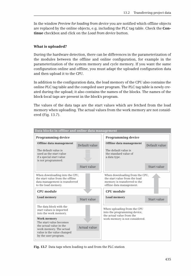
13.2 Transferring project data
435
In the window Preview for loading from device you are notified which offline objectsare replaced by the online objects, e.g. including the PLC tag table. Check the Con-tinue checkbox and click on the Load from device button.
What is uploaded?
During the hardware detection, there can be differences in the parameterization ofthe modules between the offline and online configuration, for example in theparameterization of the system memory and cycle memory. If you want the sameconfiguration online and offline, you must adapt the uploaded configuration dataand then upload it to the CPU.
In addition to the configuration data, the load memory of the CPU also contains theonline PLC tag table and the compiled user program. The PLC tag table is newly cre-ated during the upload; it also contains the names of the blocks. The names of theblock-local tags are present in the block's program.
The values of the data tags are the start values which are fetched from the loadmemory when uploading. The actual values from the work memory are not consid-ered (Fig. 13.7).
Fig. 13.7 Data tags when loading to and from the PLC station
Start value Start value
Start value Start value
Actual value
Default value Default valueOffline data management Offline data management
Programming device Programming device
CPU module CPU module
Load memory Load memory
Work memory
The default value is used as the start value if a special start value is not programmed.
The default value is the standard value of a data type.
When downloading into the CPU, the start value from the offline data management is transferred to the load memory.
When downloading from the CPU, the start value from the load memory is transferred to the offline data management.
When uploading from the CPU into the programming device, the actual value from the work memory is not considered.
The data block with the start values is imported into the work memory.
Data blocks in offline and online data management
The start value becomes the actual value in the work memory. The actual value is the value changed by the user program.

13 Online operation, diagnostics and debugging
436
You have access to the actual values in the work memory
b by directly monitoring the actual values (Chapter 13.4.5 “Monitoring of data tags” on page 446),
b with a watch table (13.4.6 “Testing with watch tables” on page 447) and
b via a program with WRIT_DBL (copying a data block with the actual values into the load memory, where the actual values then become start values).
13.3 Hardware diagnostics
The hardware diagnostics detects and signals module faults, e.g. failure of loadvoltage or open-circuit with signal modules.
The modules with diagnostics capability distinguish between parameterizable andnon-parameterizable diagnostic events. With the parameterizable diagnosticsevents, a message is only output if you enable the diagnostics in the parameter set-tings. The non-parameterizable diagnostic events are always signaled irrespectiveof the diagnostics enable.
With a diagnostics event to be signaled,
b the ERROR LED lights up on the CPU module
b the diagnostics event is sent to the CPU's operating system, and
b a diagnostics interrupt is triggered if you have enabled it in the parameter settings (in the default setting, the diagnostics interrupts are disabled).
All diagnostic events signaled to the CPU's operating system are entered in a diag-nostics buffer in the order in which they occurred with date and time (see Chapter13.3.3 “Diagnostics buffer” on page 437). In addition to the diagnostics buffer,which saves the events in chronological order, the programming device offers com-prehensive information functions which display the current module states.
13.3.1 Status displays on the modules
The status displays on the modules signal malfunctions and help to locate thefaults.
The CPU's operating system indicates malfunctions as follows:
b The ERROR LED lights up permanently.The CPU hardware is faulty.
b The ERROR LED flashes.Possible causes are an internal fault in the CPU or a configuration error (the configured hardware configuration does not agree with the actual hardware configuration).
b The RUN/STOP LED lights up yellow.The CPU does not enter RUN mode when switched on or goes to the STOP mode during RUN mode. Possible causes: Manual change in mode through the programming device, set startup type (“Startup – STOP”), STP function
13.3 Hardware diagnostics
437
in user program, system response to an execution error in the program. The events triggering the STOP mode are entered into the diagnostics buffer (see Chapter 13.3.3 “Diagnostics buffer” on page 437).
Each input/output channel of a digital module shows by means of a green status LEDwhether voltage is present at the input or output channel. This can be used, for ex-ample, to check the wiring from the sensor to the digital input channel or from thedigital output channel to the actuator.
An appropriately designed input/output channel of an analog module indicates bymeans of a green status LED that the channel has been configured and is active. Ared LED indicates a faulty analog channel or one which is not ready. For example, awire-break or short-circuit could be present. If the LED flashes red, the load voltageis missing or an I/O error is present if the diagnostics is activated.
In addition, the modules have a DIAG LED. When permanently green, this indicatesthat the module is ready. If the DIAG LED flashes green, the module is not config-ured. If the LED flashes red, a module fault exists, e.g. the load voltage is missing.
13.3.2 Diagnostics information
The diagnostics information is displayed in the work window if the programmingdevice is switched to online mode using the Online & Diagnostics command.The following diagnostics information is then available:
b General: module names, module and vendor information.
b Diagnostic status: status information of the selected module, e.g. Module exists and OK, differences between configured and existing modules.
b Cycle time: Display of preset or configured cycle (monitoring) time and minimum cycle time and – in RUN mode – the cycle time diagram and the shortest, current, and longest cycle (processing) times.
b Memory: display of utilization for the load, work and retentive memories.
b Diagnostics buffer: display of diagnostics buffer content.
If the CPU is still without a user program, it is in STOP mode. The cycle time andmemory utilization then indicate zero values.
13.3.3 Diagnostics buffer
The diagnostics buffer contains the faults detected by the CPU and the moduleswith diagnostic capability, the triggered hardware and diagnostic interrupts, andthe changes in CPU modes in the sequence of occurrence. Up to 50 entries can bestored. If more entries are present, the oldest entries are overwritten (ring bufferprinciple). If the operating voltage is switched off and on again, the last 10 entries(the most recent ones) are retained. The entries can only be erased by resetting theCPU to its factory settings (Fig. 13.8).
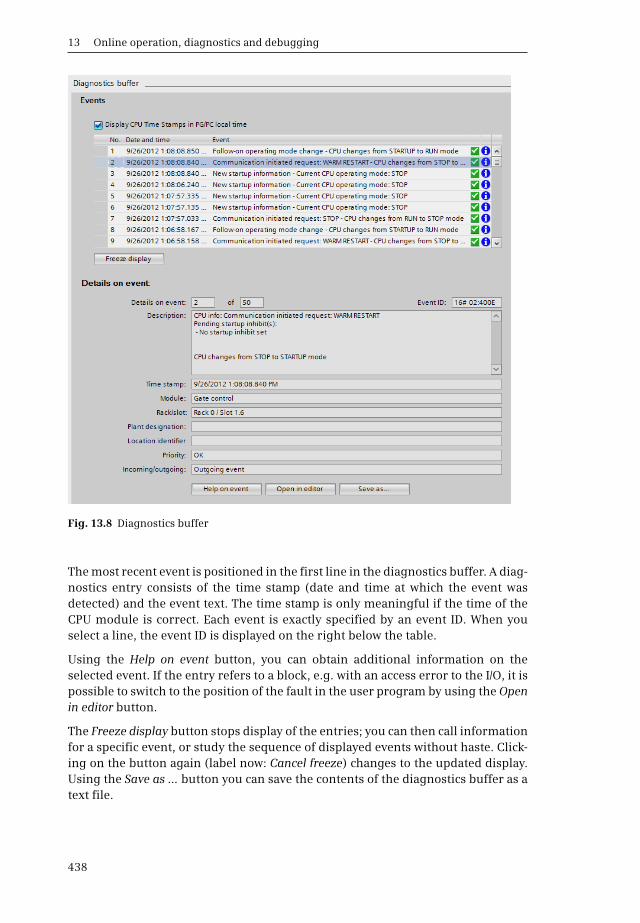
13 Online operation, diagnostics and debugging
438
The most recent event is positioned in the first line in the diagnostics buffer. A diag-nostics entry consists of the time stamp (date and time at which the event wasdetected) and the event text. The time stamp is only meaningful if the time of theCPU module is correct. Each event is exactly specified by an event ID. When youselect a line, the event ID is displayed on the right below the table.
Using the Help on event button, you can obtain additional information on theselected event. If the entry refers to a block, e.g. with an access error to the I/O, it ispossible to switch to the position of the fault in the user program by using the Openin editor button.
The Freeze display button stops display of the entries; you can then call informationfor a specific event, or study the sequence of displayed events without haste. Click-ing on the button again (label now: Cancel freeze) changes to the updated display.Using the Save as … button you can save the contents of the diagnostics buffer as atext file.
Fig. 13.8 Diagnostics buffer

13.3 Hardware diagnostics
439
13.3.4 Diagnostics functions
You can start the diagnostics functions in online mode using the Online & Diagnosticscommand from the project tree.
b Assign IP address: Setting of the IP address, subnet mask, router address.
b Set time of day: Display of programming device and module time, setting of real-time clock on CPU.
b Reset to factory settings: The user memory, operand areas, and diagnostics buffer are deleted, all parameters including the time are reset to the default settings, and the IP address is also deleted or retained depending on the pre-selection.
b Assign name: Setting a device name for a PROFINET IO device.
13.3.5 Online tools
You can start the task card with the online tools using the Online & Diagnostics com-mand from the project tree:
CPU operator panel: The CPU operator panel shows the current status of the LEDs on the front panel ofthe CPU. The RUN and STOP buttons can be used to set the CPU – following confir-mation – to the corresponding state. A pressed (darker) button symbolizes the cur-rently set state. A CPU without a user program, e.g. after being reset to the factorysettings, does not start up.
Memory reset: The MRES button is used to trigger a memory reset. A memory reset can only be car-ried out in the STOP mode. During the memory reset, the contents of the workmemory, retentive memory, and all operand areas are deleted. The contents of theload memory are retained, even if present on a memory card. The contents of theload memory relevant to execution are copied into the work memory, just like whentransferring the user program to the CPU. The diagnostics buffer, time, force jobs,and IP address remain uninfluenced.
The existing (logical) connections to the CPU module are canceled. Following a CPUmemory reset, the programming device must be switched to online mode againusing the Online & Diagnostics or Go online command.
Cycle time: Cycle time displays the shortest, current and longest cycle (processing) time in mil-liseconds, also graphically.
Memory: Memory displays the utilization of the load, work and retentive memories as barcharts.

13 Online operation, diagnostics and debugging
440
13.3.6 Further diagnostics information via the programming device
Diagnostics symbols in the device and network views
In online mode, the device configuration editor shows, in the device or networkview, the device status with diagnostics symbols on each PLC station connected on-line. For example, a green tick indicates that the station has not signaled any faults.The operating mode is indicated by a colored square: green for RUN and yellow forSTOP.
Diagnostic symbols in the project tree
In online mode, diagnostics symbols are also displayed in the project tree. A greentick is displayed after the name of the PLC station if everything is OK. A spanner sig-nals maintenance required (green), maintenance request (yellow), or fault (red).
The result of a comparison between offline and online project data is also displayedin the project tree. If an orange circle with an exclamation mark is displayed, thefolder contains objects which differ between the online and offline versions. Iden-tifications for individual objects have the following meaning:
b Green filled circle: everything OK
b Blue/orange filled circle: indicates that the online and offline versions of the object are different
b Blue/orange filled circle, right half (orange) filled: only the online object is present
b Blue/orange filled circle, left half (blue) filled: only the offline object is present
Device information in inspector window
The status of the devices signaled as faulty is displayed in the inspector window inthe Diagnostics > Device information tab. A device is considered to be faulty if it isinaccessible when establishing the online connection, if it signals a fault or if it isnot in RUN mode. (Fig. 13.9). Via the link in the Details column you can access theGo online dialog or the online and diagnostics view of the faulty device.
Fig. 13.9 Diagnostics tab in the inspector window
13.4 Testing the user program
441
13.4 Testing the user program
Following the establishment of a connection to a CPU and loading of the user pro-gram, you can test the entire program or parts of it, such as individual blocks. Yousupply the tags with signals and values and evaluate the information returned bythe program. If the CPU switches to STOP as the result of a fault, the diagnostics buf-fer provides support toward locating the cause.
Comprehensive programs are tested in sections. If you only wish to test one block,for example, load the block into the CPU and then call it in OB 1. If OB 1 is structuredsuch that the program can be tested in sections “from front to rear”, you can selectthe blocks or program sections to be tested in that you bypass the calls or programsections which are not to be processed, e.g. using a jump function.
The following testing functions are available:
b Test in program statusMonitor program execution directly in the program of the block and control tags
b Monitor PLC tagsMonitor the values in a PLC tag table
b Monitor data tagsMonitor the tag values in a data block
b Test with watch tablesMonitor and control the tag values in watch tables
b “Enable peripheral outputs” and “Modify now”Control peripheral outputs with CPU at STOP
b Test with force tableMonitor the tags in the force table and set to a fixed value (force).
A general prerequisite for testing the user program is an existing online connec-tion. When testing with program status, the offline and online versions of the blockmust be identical. The CPU is in RUN mode.
13.4.1 Introduction to testing with program status
The program status shows the program execution during runtime. You can monitorthe current signal status of the binary tags and the current values of digital tags.
Caution! Functional disturbances may occur as a result of program modificationswhen testing the user program during ongoing operation on the process. Make surewith each testing step that no serious damage to property or injury to persons canoccur!
Note that the program status requires significant resources, and that under certaincircumstances the test function may therefore be executed with limitations.

13 Online operation, diagnostics and debugging
442
Changing a block with the program status switched on, i.e. with an online connec-tion present, is described in Section 13.2.5 “Processing blocks offline/online” onpage 431.
Switching the program status on and off
In order to switch on the program status, open the block to be monitored and clickon the Monitoring on/off symbol in the toolbar of the work window.
If an online connection to the CPU has not yet been established, STEP 7 searches foraccessible devices. If necessary, set the interface used in the programming devicein the dialog window Go online, select the PLC station found, and click on the Goonline button.
To switch off the program status, click again on the Monitoring on/off symbol in thetoolbar. You will be asked whether the online connection created when switchingon the program status is to be disconnected. If you click on the No button, the pro-gram status is terminated but the online connection is retained.
13.4.2 Program status with LAD and FBD
The program status shows the binary signal flow and the values of digital tags di-rectly in the LAD or FBD program.
Open the block, e.g. by double-clicking in the project tree, set the network whoseprogram you wish to debug, and click on the Monitoring on/off symbol in the toolbarof the work window.
LAD program status
In the LAD program status, green continuous lines are used to identify contacts,coils, and the connections between the program elements which have signal state“1”. Program elements with signal state “0” are identified by blue dashed lines(Fig. 13.10).
Fig. 13.10 LAD program status
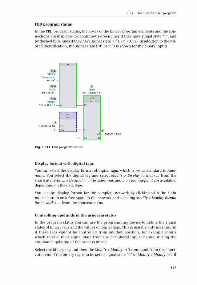
13.4 Testing the user program
443
FBD program status
In the FBD program status, the boxes of the binary program elements and the con-nections are displayed by continuous green lines if they have signal state “1”, andby dashed blue lines if they have signal state “0” (Fig. 13.11). In addition to the col-ored identification, the signal state (“0” or “1”) is shown for the binary inputs.
Display format with digital tags
You can select the display format of digital tags, which is set as standard to Auto-matic: You select the digital tag and select Modify > Display format> … from theshortcut menu. ... > Decimal, … > Hexadecimal, and … > Floating-point are available,depending on the data type.
You set the display format for the complete network by clicking with the rightmouse button on a free space in the network and selecting Modify > Display formatfor network > ... from the shortcut menu.
Controlling operands in the program status
In the program status you can use the programming device to define the signalstates of binary tags and the values of digital tags. This is usually only meaningfulif these tags cannot be controlled from another position, for example inputswhich receive their signal state from the peripheral input channel during theautomatic updating of the process image.
Select the binary tag and then the Modify > Modify to 0 command from the short-cut menu if the binary tag is to be set to signal state “0” or Modify > Modify to 1 if
Fig. 13.11 FBD program status
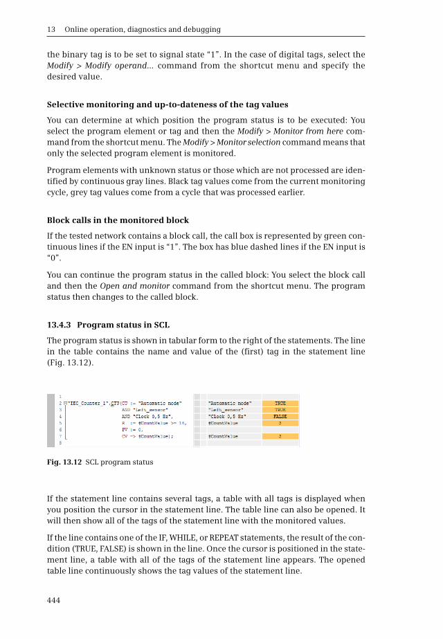
13 Online operation, diagnostics and debugging
444
the binary tag is to be set to signal state “1”. In the case of digital tags, select theModify > Modify operand… command from the shortcut menu and specify thedesired value.
Selective monitoring and up-to-dateness of the tag values
You can determine at which position the program status is to be executed: Youselect the program element or tag and then the Modify > Monitor from here com-mand from the shortcut menu. The Modify > Monitor selection command means thatonly the selected program element is monitored.
Program elements with unknown status or those which are not processed are iden-tified by continuous gray lines. Black tag values come from the current monitoringcycle, grey tag values come from a cycle that was processed earlier.
Block calls in the monitored block
If the tested network contains a block call, the call box is represented by green con-tinuous lines if the EN input is “1”. The box has blue dashed lines if the EN input is“0”.
You can continue the program status in the called block: You select the block calland then the Open and monitor command from the shortcut menu. The programstatus then changes to the called block.
13.4.3 Program status in SCL
The program status is shown in tabular form to the right of the statements. The linein the table contains the name and value of the (first) tag in the statement line(Fig. 13.12).
If the statement line contains several tags, a table with all tags is displayed whenyou position the cursor in the statement line. The table line can also be opened. Itwill then show all of the tags of the statement line with the monitored values.
If the line contains one of the IF, WHILE, or REPEAT statements, the result of the con-dition (TRUE, FALSE) is shown in the line. Once the cursor is positioned in the state-ment line, a table with all of the tags of the statement line appears. The openedtable line continuously shows the tag values of the statement line.
Fig. 13.12 SCL program status

13.4 Testing the user program
445
Addressing and display format
By clicking on the Absolute/symbolic operands in the toolbar of the working window,you can supplement the symbolic addressing or the absolute addressing or hide theabsolute address again.
You can select the display format, which is set as standard to Automatic: You selectthe tag value and select Display format > ... from the shortcut menu. ... > Decimal, ...>Hexadecimal, and ...> Floating-point are available, depending on the data type.
Modifying operands in the program status
In the program status, you can define the signal states of binary tags and the valuesof digital tags using the programming device. This is usually only meaningful ifthese tags are not controlled from another point, for example inputs which receivetheir signal state from the I/O input channel during automatic updating of the pro-cess image.
Select the binary tag and then the Modify > Modify to 0 command from the short-cut menu if the binary tag is to be set to signal state “0” or Modify > Modify to 1 ifthe binary tag is to be set to signal state “1”. In the case of digital tags, select theModify > Modify operand… command from the shortcut menu and specify thedesired value.
Up-to-dateness of the tag values
Black tag values come from the current monitoring cycle. Grey ones come from acycle that was processed earlier. If a tag value is not displayed, the correspondingtag is not processed or has an unknown status.
If no value can be shown for a tag or event due to missing compilation options, thecell in the Value column contains three question marks on a yellow background. Inthis case, activate the Create extended status information attribute in the blockproperties and load the block again into the CPU.
Block calls in the monitored block
If the tested statement line contains a block call, you can continue the program sta-tus in the called block : You select the block call and then the Monitor commandfrom the shortcut menu. The program status then changes to the called block.
13.4.4 Monitoring with the PLC tag table
To monitor the tag table, double-click on the corresponding PLC tag table. Click theMonitor all icon in the toolbar. The PLC tag table changes to online mode and theMonitor value column is displayed. You can now monitor the tag values (Fig. 13.13).
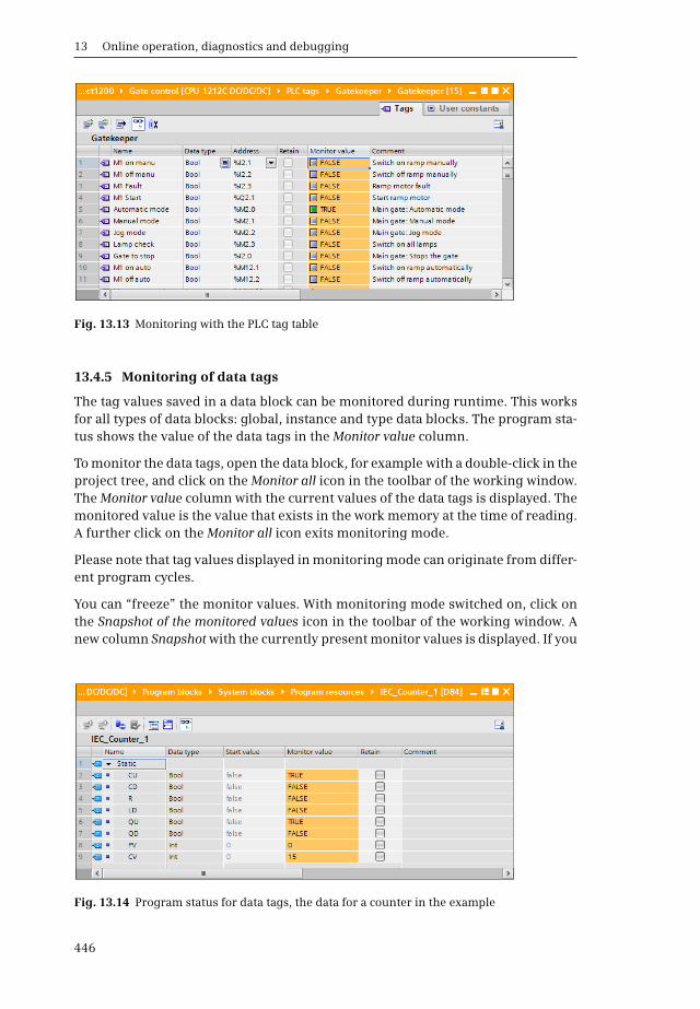
13 Online operation, diagnostics and debugging
446
13.4.5 Monitoring of data tags
The tag values saved in a data block can be monitored during runtime. This worksfor all types of data blocks: global, instance and type data blocks. The program sta-tus shows the value of the data tags in the Monitor value column.
To monitor the data tags, open the data block, for example with a double-click in theproject tree, and click on the Monitor all icon in the toolbar of the working window.The Monitor value column with the current values of the data tags is displayed. Themonitored value is the value that exists in the work memory at the time of reading.A further click on the Monitor all icon exits monitoring mode.
Please note that tag values displayed in monitoring mode can originate from differ-ent program cycles.
You can “freeze” the monitor values. With monitoring mode switched on, click onthe Snapshot of the monitored values icon in the toolbar of the working window. Anew column Snapshot with the currently present monitor values is displayed. If you
Fig. 13.13 Monitoring with the PLC tag table
Fig. 13.14 Program status for data tags, the data for a counter in the example

13.4 Testing the user program
447
would like to use the monitored actual values as start values, copy the desired val-ues from the Monitor value column into the Start value column.
Fig. 13.14 shows the monitoring function for an instance data block for a counterfunction.
13.4.6 Testing with watch tables
Watch tables contain tags whose values can be monitored and modified (controlled)during runtime. Any combination of tags is possible, and a specially tailored watchtable can therefore be created for each debugging case.
The following functions can be performed with a watch table:
b Monitor tags
b Modify tags
b Force tags
b “Enable peripheral outputs” and “Modify now”
Tags from the peripherals, inputs, outputs, and bit memory areas as well as tags fromdata blocks (global, instance, and type data blocks) can be used in watch tables.
Creating watch tables
Underneath a PLC station in the project tree there is the Watch and force tablesfolder with the watch tables and the force table. Further subfolders can be createdwithin this folder in order to structure the watch tables: Select the Watch and forcetables folder and then the Add group command from the shortcut menu. You canassign separate names to the new subfolders and the watch tables by using theRename command from the shortcut menu.
In order to create a new watch table, double-click on the Add new watch table com-mand. In the empty table, enter the names of the tags line by line and the display
Fig. 13.15 Example of monitoring of tags in expanded mode
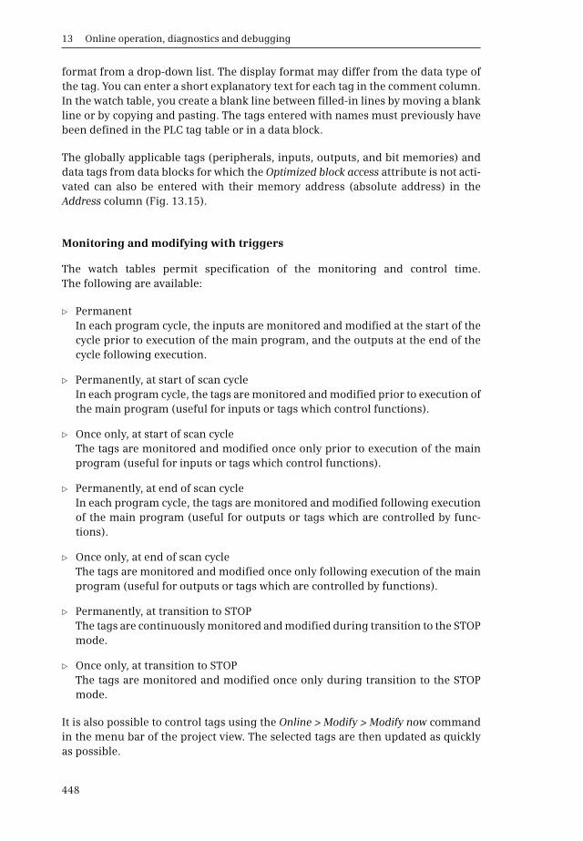
13 Online operation, diagnostics and debugging
448
format from a drop-down list. The display format may differ from the data type ofthe tag. You can enter a short explanatory text for each tag in the comment column.In the watch table, you create a blank line between filled-in lines by moving a blankline or by copying and pasting. The tags entered with names must previously havebeen defined in the PLC tag table or in a data block.
The globally applicable tags (peripherals, inputs, outputs, and bit memories) anddata tags from data blocks for which the Optimized block access attribute is not acti-vated can also be entered with their memory address (absolute address) in theAddress column (Fig. 13.15).
Monitoring and modifying with triggers
The watch tables permit specification of the monitoring and control time.The following are available:
b PermanentIn each program cycle, the inputs are monitored and modified at the start of thecycle prior to execution of the main program, and the outputs at the end of thecycle following execution.
b Permanently, at start of scan cycleIn each program cycle, the tags are monitored and modified prior to execution ofthe main program (useful for inputs or tags which control functions).
b Once only, at start of scan cycleThe tags are monitored and modified once only prior to execution of the mainprogram (useful for inputs or tags which control functions).
b Permanently, at end of scan cycleIn each program cycle, the tags are monitored and modified following executionof the main program (useful for outputs or tags which are controlled by func-tions).
b Once only, at end of scan cycleThe tags are monitored and modified once only following execution of the mainprogram (useful for outputs or tags which are controlled by functions).
b Permanently, at transition to STOPThe tags are continuously monitored and modified during transition to the STOPmode.
b Once only, at transition to STOPThe tags are monitored and modified once only during transition to the STOPmode.
It is also possible to control tags using the Online > Modify > Modify now commandin the menu bar of the project view. The selected tags are then updated as quicklyas possible.
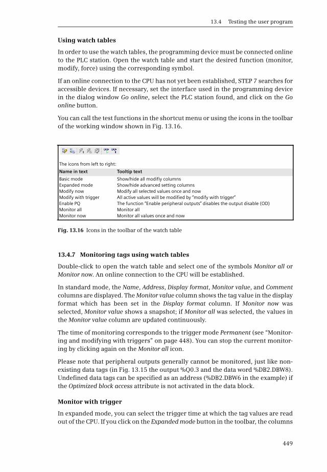
13.4 Testing the user program
449
Using watch tables
In order to use the watch tables, the programming device must be connected onlineto the PLC station. Open the watch table and start the desired function (monitor,modify, force) using the corresponding symbol.
If an online connection to the CPU has not yet been established, STEP 7 searches foraccessible devices. If necessary, set the interface used in the programming devicein the dialog window Go online, select the PLC station found, and click on the Goonline button.
You can call the test functions in the shortcut menu or using the icons in the toolbarof the working window shown in Fig. 13.16.
13.4.7 Monitoring tags using watch tables
Double-click to open the watch table and select one of the symbols Monitor all orMonitor now. An online connection to the CPU will be established.
In standard mode, the Name, Address, Display format, Monitor value, and Commentcolumns are displayed. The Monitor value column shows the tag value in the displayformat which has been set in the Display format column. If Monitor now wasselected, Monitor value shows a snapshot; if Monitor all was selected, the values inthe Monitor value column are updated continuously.
The time of monitoring corresponds to the trigger mode Permanent (see “Monitor-ing and modifying with triggers” on page 448). You can stop the current monitor-ing by clicking again on the Monitor all icon.
Please note that peripheral outputs generally cannot be monitored, just like non-existing data tags (in Fig. 13.15 the output %Q0.3 and the data word %DB2.DBW8).Undefined data tags can be specified as an address (%DB2.DBW6 in the example) ifthe Optimized block access attribute is not activated in the data block.
Monitor with trigger
In expanded mode, you can select the trigger time at which the tag values are readout of the CPU. If you click on the Expanded mode button in the toolbar, the columns
The icons from left to right:
Name in text Tooltip text
Basic modeExpanded modeModify nowModify with triggerEnable PQMonitor allMonitor now
Show/hide all modifiy columnsShow/hide advanced setting columnsModify all selected values once and nowAll active values will be modified by “modify with trigger”The function “Enable peripheral outputs” disables the output disable (OD)Monitor allMonitor all values once and now
Fig. 13.16 Icons in the toolbar of the watch table

13 Online operation, diagnostics and debugging
450
Monitor with trigger and Modify with trigger are displayed. You can then define theread time for each tag from a drop-down list.
Tag values which are read out once only or which are not read out (yet) are shownin the Monitor value column with a gray background; permanently read values havean orange background
Fig. 13.5 on page 432 shows an example of monitoring with watch table in extendedmode.
13.4.8 Modifying tags using watch tables
Double-click to open the watch table and select the symbol Basic mode. In additionto the Name, Address, Display format, Monitor value, and Comment columns, theModify value and Tag selection (represented by a lightning icon) columns are nowdisplayed (Fig. 13.17).
Enter the value to which the tag is to be set in the Modify value column, and activatethe check box in the Tag selection column if the associated tag is to be modified.A yellow triangle with exclamation mark indicates that the selected tag has not yetbeen modified.
It is recommendable to switch on monitoring mode prior to modification. An onlineconnection to the CPU is then already made, and the effects of modification can bemonitored.
Caution! Make sure when modifying tags that no dangerous states can result!
To modify the activated tags, click on the symbol Modify now. The tags activated inthe Tag selection column are immediately set (as fast as possible) to the controlvalue. If a tag is immediately overwritten after the modification by a value from theprogram – for example if a switched-on input has been controlled to “0” and the
Fig. 13.17 Example of controlling tags with an error message

13.4 Testing the user program
451
process image updating overwrites the control value again – the yellow triangleappears again in the Tag selection column.
Alternatively, modification can be triggered by means of the Online > Modify > Mod-ify now command from the main menu or the Modify > Modify now command fromthe shortcut menu. The Modify > Modify to 0 and Modify > Modify to 1 commandsfrom the shortcut menu immediately control the binary tag selected in the watchtable.
Please note that peripheral inputs can never be modified (in Fig. 13.17 the periph-eral inputs %I1.0:P and %I1.7:P). Only the tags visible in the table are modified.Multiple controlling of a tag or parts of a tag in the monitor table is not allowed (inthe figure: the data bit %DB2.DBX6.0 and the data word %DB2.DBW6).
Modifying with triggers
In expanded mode, you can select the trigger time at which the tag values are mod-ified in the CPU. If you click on the Expanded mode button in the toolbar, the col-umns Monitor with trigger and Modify with trigger are displayed. You can then definethe control time for each tag from a drop-down list.
If you click the symbol Modify with trigger, all activated tags are updated (followingconfirmation) with the control value in accordance with the trigger conditions.Clicking on the icon again exits permanent control.
Alternatively, modifying can be triggered or terminated using the Online > Modify> Modify with trigger command from the main menu or the Modify > Modify withtrigger command from the command menu.
13.4.9 Enable peripheral outputs and “Modify now”
In STOP mode, the output modules are normally disabled by the OD signal (com-mand output disable); the Enable peripheral outputs (PQ) function can be used toswitch off the OD signal so that you can also control the output modules with theCPU at STOP. Controlling is carried out using a watch table. An application for thiswould be checking the wiring of the outputs in STOP mode and without a user pro-gram.
Caution! Make sure that no dangerous states can occur with “Enable peripheraloutputs”!
Prerequisites for Enable peripheral outputs: An online connection exists to the CPUwhich is in the STOP mode. A watch table with the peripheral outputs to be con-trolled has been created and expanded mode is switched on. Exit all force jobs (seenext Chapter)!
Open the watch table, click on the Basic mode icon, enter the control value in theModify value column, and activate the selection checkbox. You switch off the com-mand output disable (OD) for the output modules via the Enable PQ icon in the tool-bar. You can now control the tags using the Modify now icon. Alternatively you can

13 Online operation, diagnostics and debugging
452
use the Online > Modify > Enable peripheral outputs and Online > Modify > Modifynow commands from the main menu (Fig. 13.18).
You can then control the peripheral outputs for as long as Enable peripheral outputsis switched on.
You deactivate the Enable peripheral outputs function – the OD signal is thenswitched on again – by selecting the Enable PQ function again, by changing the CPUmode, or by canceling the online connection.
13.4.10 Forcing tags
Tags can be preassigned fixed values. This action is referred to as forcing. A CPU1200 can force tags out of the I/O area, i.e. assign a peripheral input with signalstate “0” or “1”, regardless of the voltage at the input terminal, or a peripheral out-put (the output terminal) with a signal state of “0” or “1” regardless of the programfunction. The tags to be forced are entered in the force table. The force table is pres-ent once for a CPU and cannot be copied or renamed. Forcing is then only possibleif the Enable peripheral outputs function is deactivated.
Please note the following special features when using the force function: forcing issent to the CPU by means of a force job. The force job remains active even if onlinemode has been terminated and the online connection to the programming device can-celed!
The force job also remains active when the CPU is switched off and on again! Forcingcan only be terminated by the Online > Force > Stop forcing command; this com-mand deletes the force job in the CPU.
You can call the test functions when forcing from the shortcut menu or using theicons in the toolbar of the working window shown in Fig. 13.19.
Fig. 13.18 Example for Enable PQ and Modify now
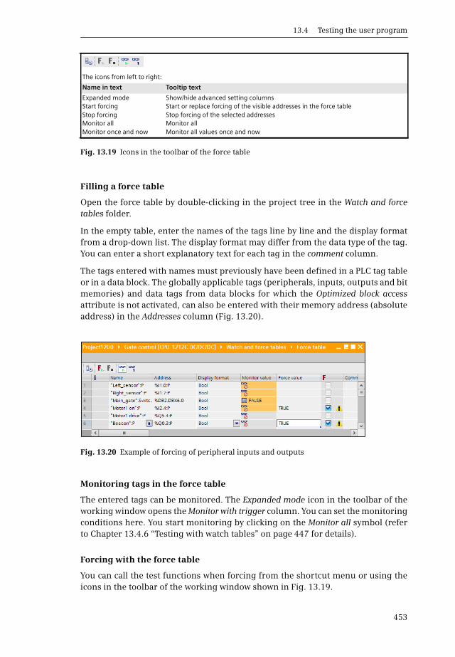
13.4 Testing the user program
453
Filling a force table
Open the force table by double-clicking in the project tree in the Watch and forcetables folder.
In the empty table, enter the names of the tags line by line and the display formatfrom a drop-down list. The display format may differ from the data type of the tag.You can enter a short explanatory text for each tag in the comment column.
The tags entered with names must previously have been defined in a PLC tag tableor in a data block. The globally applicable tags (peripherals, inputs, outputs and bitmemories) and data tags from data blocks for which the Optimized block accessattribute is not activated, can also be entered with their memory address (absoluteaddress) in the Addresses column (Fig. 13.20).
Monitoring tags in the force table
The entered tags can be monitored. The Expanded mode icon in the toolbar of theworking window opens the Monitor with trigger column. You can set the monitoringconditions here. You start monitoring by clicking on the Monitor all symbol (referto Chapter 13.4.6 “Testing with watch tables” on page 447 for details).
Forcing with the force table
You can call the test functions when forcing from the shortcut menu or using theicons in the toolbar of the working window shown in Fig. 13.19.
The icons from left to right:
Name in text Tooltip text
Expanded modeStart forcingStop forcingMonitor allMonitor once and now
Show/hide advanced setting columnsStart or replace forcing of the visible addresses in the force tableStop forcing of the selected addressesMonitor allMonitor all values once and now
Fig. 13.19 Icons in the toolbar of the force table
Fig. 13.20 Example of forcing of peripheral inputs and outputs

13 Online operation, diagnostics and debugging
454
To carry out forcing, enter a value in the Force value column and activate the check-box in the Force column (tag selection depicted by a red “F”). A yellow triangle withexclamation mark indicates that the selected tag has not yet been forced.
It is recommendable to switch on monitoring mode prior to forcing. An online con-nection to the CPU is then already made, and the effects of forcing can be moni-tored.
Caution: Make sure when forcing tags that no dangerous states can result!
The Start forcing icon sends a force job to the CPU which contains the tags selectedfor forcing. Forcing is effective immediately. A forced tag is marked with a red “F”in the first column of the watch table. It is not possible to force parts of a tag, forexample of individual peripheral bits, if the peripheral byte is already being forced.
To exit forcing for individual tags, deactivate the checkbox in the tag selection andclick on the Start forcing icon again. A new force job is sent to the CPU which termi-nates forcing for the tags which are no longer selected.
You exit forcing for all tags using the Stop forcing icon. A new force job is sent to theCPU which terminates forcing for all forced tags.
Note that termination of forcing leave the tags in their last state! Only the force job isdeleted. For example, an output of a digital module remains in signal state “1” aftertermination of forcing if it is not controlled otherwise by the program.
As an alternative to forcing using the icons, you can select one or more tags in theforce table and then the Force > Force to 0, Force > Force to 1, Force > Force all, andForce > Stop forcing commands from the shortcut menu or the commands from themain menu under menu item Online > Force > … .
Forcing in association with memory card
The offline project data that is copied to a memory card (program or transfer card)does not contain any force jobs. If the user program is transferred from a memorycard to the CPU, the force jobs are deleted in the internal load memory.
If an empty program card is plugged in and the user program is copied from theinternal load memory into the memory card, which is then used as an external loadmemory, the force jobs are also copied.
If a program card is plugged in during runtime and force jobs are set up, the forcejobs are saved on the memory card (in the external load memory).
Usage of the memory card is described in Chapter 13.2.4 “Working with the mem-ory card” on page 428.

455
14 Distributed I/O
14.1 Introduction, overview
Distributed I/O is the term used for input/output modules connected to the centralPLC station over a bus system. SIMATIC S7 uses the PROFINET IO, PROFIBUS DP, andAS-Interface (AS-i) bus systems.
The distributed I/O is handled like the central I/O. The distributed inputs/outputsare in the same address volume as the central inputs/outputs, and therefore theaddresses of the distributed I/O must not overlap with those of the central I/O. Thedistributed I/Os can be addressed via the following operand areas: peripheralinputs (I:P) and peripheral outputs (Q:P) and – if they are present in the processimage – also via the inputs (I) and outputs (Q).
Transfer between the distributed modules and the central CPU is carried out “auto-matically” and you need not take this into account when addressing.
Data transfer to and from the distributed I/O is controlled from a central point:With PROFINET IO it is the IO controller, with PROFIBUS DP it is the DP master, andwith AS-Interface it is the AS-i master. The distributed stations – these are the IOdevices with PROFINET IO, the DP slaves with PROFIBUS DP, and the AS-i slaves withAS-Interface – are the passive partners in the data transfer.
S7 stations and ET200 stations with a CPU can also be used as distributed I/O sta-tions and these are then “intelligent” DP slaves or IO devices. While these stationsare controlling their own modules (considered from their viewpoint as centralmodules), they also satisfy – when working at the same time as IO devices or DPslaves – the data requirements of the respective IO controller or DP master.
The distributed I/O is configured using the hardware configuration. PROFINET IO,PROFIBUS DP (with the CM 1243-5 module as the DP master) and AS-Interface (withthe CM 1243-2 module as the AS-i master) are handled like subnets, in which theconnections needed for the data transfer are “automatically” available.
Network transitions between the subnets can be produced using link and couplermodules which allow data exchange between the stations connected to the variousnetworks. The programming device is able to handle programming and servicingfunctions over PROFINET IO and PROFIBUS DP. It can reach all (“intelligent”) sta-tions connected to the subnets if the subnet gateways are present in stations withrouting capability.
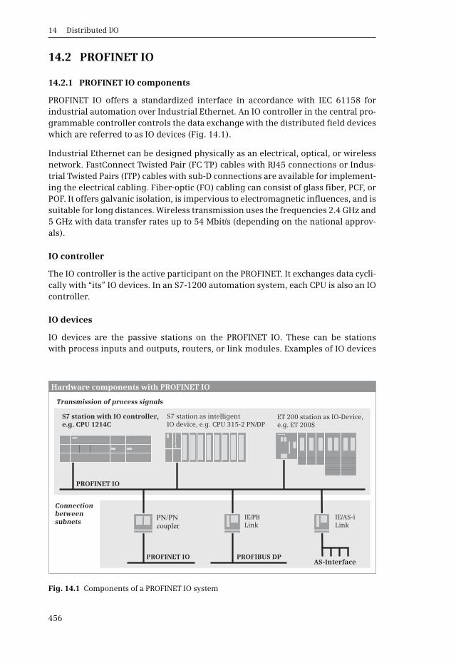
14 Distributed I/O
456
14.2 PROFINET IO
14.2.1 PROFINET IO components
PROFINET IO offers a standardized interface in accordance with IEC 61158 forindustrial automation over Industrial Ethernet. An IO controller in the central pro-grammable controller controls the data exchange with the distributed field deviceswhich are referred to as IO devices (Fig. 14.1).
Industrial Ethernet can be designed physically as an electrical, optical, or wirelessnetwork. FastConnect Twisted Pair (FC TP) cables with RJ45 connections or Indus-trial Twisted Pairs (ITP) cables with sub-D connections are available for implement-ing the electrical cabling. Fiber-optic (FO) cabling can consist of glass fiber, PCF, orPOF. It offers galvanic isolation, is impervious to electromagnetic influences, and issuitable for long distances. Wireless transmission uses the frequencies 2.4 GHz and5 GHz with data transfer rates up to 54 Mbit/s (depending on the national approv-als).
IO controller
The IO controller is the active participant on the PROFINET. It exchanges data cycli-cally with “its” IO devices. In an S7-1200 automation system, each CPU is also an IOcontroller.
IO devices
IO devices are the passive stations on the PROFINET IO. These can be stationswith process inputs and outputs, routers, or link modules. Examples of IO devices
Fig. 14.1 Components of a PROFINET IO system
PROFINET IO
PROFINET IO
Hardware components with PROFINET IO
PROFIBUS DPAS-Interface
IE/PBLink
Transmission of process signals
IE/AS-iLink
PN/PNcoupler
S
S
S7 station with IO controller, e.g. CPU 1214C
S7 station as intelligent IO device, e.g. CPU 315-2 PN/DP
ET 200 station as IO-Device, e.g. ET 200S
Connection between subnets
S
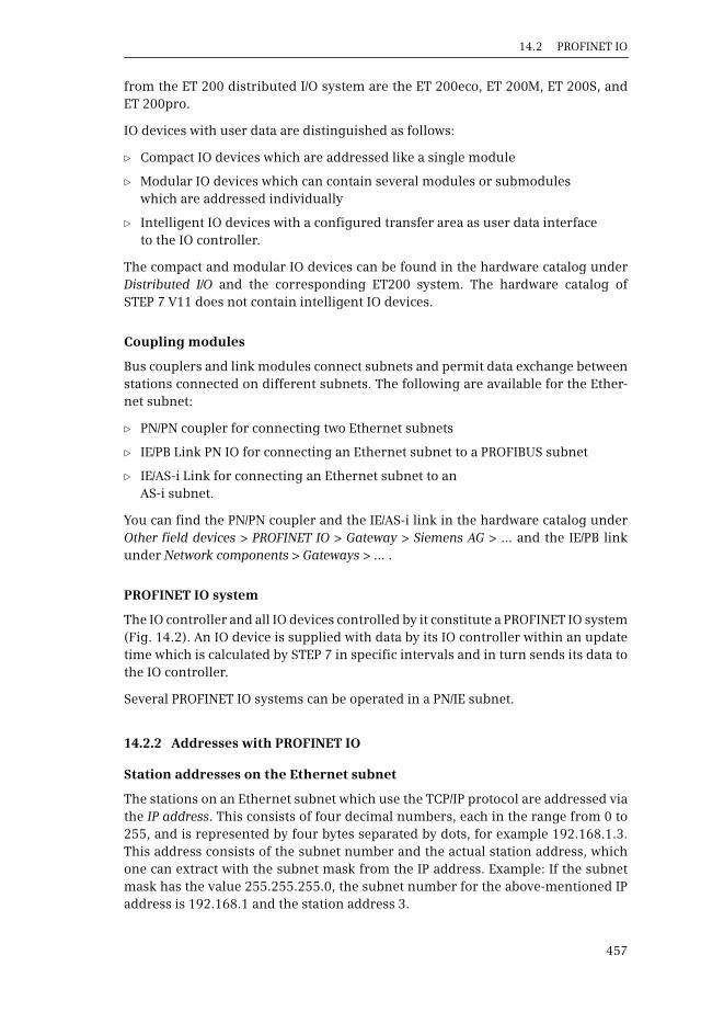
14.2 PROFINET IO
457
from the ET 200 distributed I/O system are the ET 200eco, ET 200M, ET 200S, andET 200pro.
IO devices with user data are distinguished as follows:
b Compact IO devices which are addressed like a single module
b Modular IO devices which can contain several modules or submodules which are addressed individually
b Intelligent IO devices with a configured transfer area as user data interface to the IO controller.
The compact and modular IO devices can be found in the hardware catalog underDistributed I/O and the corresponding ET200 system. The hardware catalog ofSTEP 7 V11 does not contain intelligent IO devices.
Coupling modules
Bus couplers and link modules connect subnets and permit data exchange betweenstations connected on different subnets. The following are available for the Ether-net subnet:
b PN/PN coupler for connecting two Ethernet subnets
b IE/PB Link PN IO for connecting an Ethernet subnet to a PROFIBUS subnet
b IE/AS-i Link for connecting an Ethernet subnet to an AS-i subnet.
You can find the PN/PN coupler and the IE/AS-i link in the hardware catalog underOther field devices > PROFINET IO > Gateway > Siemens AG > ... and the IE/PB linkunder Network components > Gateways > … .
PROFINET IO system
The IO controller and all IO devices controlled by it constitute a PROFINET IO system(Fig. 14.2). An IO device is supplied with data by its IO controller within an updatetime which is calculated by STEP 7 in specific intervals and in turn sends its data tothe IO controller.
Several PROFINET IO systems can be operated in a PN/IE subnet.
14.2.2 Addresses with PROFINET IO
Station addresses on the Ethernet subnet
The stations on an Ethernet subnet which use the TCP/IP protocol are addressed viathe IP address. This consists of four decimal numbers, each in the range from 0 to255, and is represented by four bytes separated by dots, for example 192.168.1.3.This address consists of the subnet number and the actual station address, whichone can extract with the subnet mask from the IP address. Example: If the subnetmask has the value 255.255.255.0, the subnet number for the above-mentioned IPaddress is 192.168.1 and the station address 3.
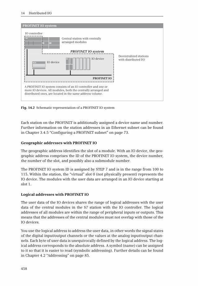
14 Distributed I/O
458
Each station on the PROFINET is additionally assigned a device name and number.Further information on the station addresses in an Ethernet subnet can be foundin Chapter 3.4.5 “Configuring a PROFINET subnet” on page 73.
Geographic addresses with PROFINET IO
The geographic address identifies the slot of a module. With an IO device, the geo-graphic address comprises the ID of the PROFINET IO system, the device number,the number of the slot, and possibly also a submodule number.
The PROFINET IO system ID is assigned by STEP 7 and is in the range from 100 to115. Within the station, the “virtual” slot 0 (not physically present) represents theIO device. The modules with the user data are arranged in an IO device starting atslot 1.
Logical addresses with PROFINET IO
The user data of the IO devices shares the range of logical addresses with the userdata of the central modules in the S7 station with the IO controller. The logicaladdresses of all modules are within the range of peripheral inputs or outputs. Thismeans that the addresses of the central modules must not overlap with those of theIO devices.
You use the logical address to address the user data, in other words the signal statesof the digital input/output channels or the values at the analog input/output chan-nels. Each byte of user data is unequivocally defined by the logical address. The log-ical address corresponds to the absolute address. A symbol (name) can be assignedto it so that it is easier to read (symbolic addressing). Further details can be foundin Chapter 4.2 “Addressing” on page 85.
Fig. 14.2 Schematic representation of a PROFINET IO system
S
IO device
IO controller
IO device
PROFINET IO
PROFINET IO system
PROFINET IO system
Central station with centrally arranged modules
Decentralized stations with distributed I/O
A PROFINET IO system consists of an IO controller and one or more IO devices. All modules, both the centrally arranged and distributed ones, are located in the same address volume.
14.2 PROFINET IO
459
Consistent user data transfer to and from IO devices
Data consistency means that a block of user data is handled together. WithPROFINET IO a CPU 1200 transfers a data block with up to 64 bytes consistently. Iflonger data blocks are to be consistently transferred, use the system functionDPRD_DAT for reading and DPWR_DAT for writing. These system functions aredescribed in Chapter 14.3.4 “System functions for PROFINET IO and PROFIBUS DP”on page 470.
The handling of consistent user data areas in the user memory is described inChapter 4.1.2 „Operand areas: inputs and outputs“ in Section “Consistent user dataareas” on page 81.
14.2.3 Configuring PROFINET IO
General procedure
A prerequisite for configuration of the distributed I/O with PROFINET IO is a createdproject with a PLC station. To select the stations involved, start the hardware con-figuration in the Network view.
b The starting point for the configuration is the IO controller in a CPU 1200. The IO controller mode is preset.
b Assign a PROFINET IO system to the PN interface of the IO controller. The Ethernet subnet required is created automatically in the process.
b Select an IO device from the hardware catalog and drag it with the mouse into the working window.
b Link the IO device to the PROFINET IO system by dragging the PN interface of the IO device with the mouse to the PN interface of the IO controller.
b Repeat the three steps for every further IO device.
b To parameterize a PN interface, select it in the working window and set the desired properties in the inspector window.
The result is networking of the IO controller with the assigned IO devices to aPROFINET IO system (Fig. 14.3).
Fig. 14.3 Example of representation of a PROFINET IO system

14 Distributed I/O
460
You then make the parameter settings for the stations and the fitting withinput/output modules in the Device view.
Configuring the IO controller in the Network view
Prerequisite: You have created a project and a PLC station, for example a CPU 1200.Start the device configuration and select the Network view tab in the working win-dow.
Select the PN interface shown in green in the graphic of the CPU and then the Ether-net addresses group in the Properties tab in the inspector window. Activate the SetIP address in project option and change the preset IP address and subnet mask ifnecessary. Information on the IP address can be found in Chapter 3.4.5 “Configur-ing a PROFINET subnet” on page 73. Activate the Set PROFINET device name using adifferent method option if you wish, for example, to set the IP address per user pro-gram.
Connect the PN interface to a PROFINET subnet. You can do this in the properties ofthe PN interface: Select an existing subnet under Ethernet address in the Subnetdrop-down list or create a new subnet using the Add new subnet button. You canalso click on the PN interface with the right mouse button and select the Add subnetcommand from the shortcut menu. A green subnet is shown with the name PN/IE_x.You can change the name in the subnet properties.
Configure a PROFINET IO system. To do this, click with the right mouse button onthe PN interface and select the Assign IO system command from the shortcut menu.A green/white marking is shown with the name <Station name>.PROFINET IO system(xxx). xxx is the number of the IO system. You can change the name and number inthe properties of the PROFINET IO system.
Adding an IO device to the IO system
With the left mouse button pressed, drag the desired IO device from the hardwarecatalog to the IO system on the working area. Fig. 14.3 shows three stations of thedistributed I/O: an ET 200M station from the object tree Distributed I/O > ET 200M >Interface modules > PROFINET > IM 153-4 PN > ... , an ET200eco station from theobject tree Distributed I/O > ET 200eco PN > Compact modules PROFINET > DI/DO >8DIO x DC24V / 1.3A 8xM12 > … and an ET 200S station from the object tree Distrib-uted I/O > ET 200S > Interface modules > PROFINET > IM 151-3 PN > … .
The interfaces of the IO devices are connected in the graphic with the green/whitemarking and are thus part of the PROFINET IO system.
The automatically assigned station name is applied as the PROFINET device name.You can change the name in the station properties and also the device number andIP address.
Configuring an IO device
With the IO device selected, you can set its properties in the inspector window in theDevice view. You fit a modular IO device with the desired modules or submodulesfrom the hardware catalog and then set their parameters.

14.2 PROFINET IO
461
In the properties of the PROFINET interface, set the Ethernet addresses. Set thedesired application in the Advanced options group.
14.2.4 Real-time communication with PROFINET IO
PROFINET IO offers several types of data transfer:
b Non-time-critical data such as configuration and diagnostic information is transferred acyclically with the TCP/IP communication standard.
b User data (input/output information) is exchanged cyclically between the IO con-troller and the IO device (real-time RT) within a defined time period – the update time.
b Time-critical user data, e.g. for motion control applications, is transferred iso-chronously with hardware support (isochronous real-time IRT).
A permanent communication channel is reserved on the Ethernet subnet for IRTcommunication. RT communication – cyclic data exchange between the IO Control-ler and IO Devices – and non-real-time TCP/IP communication take place parallel tothe update time. In this way, all three communication types can exist in parallel onthe same subnet.
The configuration of IRT communication is not possible with STEP 7 V11.
Send clock in the PROFINET IO system
Cyclic data exchange is handled within a specific time frame, the send clock. STEP 7calculates the send clock from the configuration information on the PROFINET IOsystem. The send clock is the shortest possible update time.
You configure the send clock in the interface properties of the IO controller. Withthe PN interface selected, select a value in the properties tab under Advanced > Realtime settings > IO communication from the drop-down list Shortest possible updateinterval.
Update time and watchdog timer for IO devices
The update time is the period within which each IO device in the IO system hasexchanged its user data with the IO controller. The update time corresponds to thesend clock or a multiple thereof. You can increase the update time manually, forexample to reduce the bus load. Under certain circumstances, you can reduce theupdate time for individual IO devices if you in return increase the update time forother devices whose user data can be exchanged non-time-critically.
If the IO device is not supplied by the IO controller with input or output data withinthe watchdog timer, it switches to a safe state. The watchdog timer is calculated asthe product of the update time and “Accepted update cycles without IO data”.
You configure the times in the interface properties of the IO device. To do this,select the IO device and then the PROFINET interface > Advanced options > Real timesettings > IO cycle group in the properties tab. Under Update time, select the Can beset option and then the update time from the drop-down list. To achieve automatic
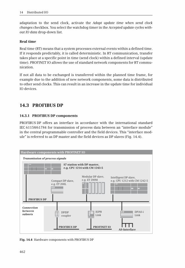
14 Distributed I/O
462
adaptation to the send clock, activate the Adapt update time when send clockchanges checkbox. You select the watchdog timer in the Accepted update cycles with-out IO data drop-down list.
Real time
Real time (RT) means that a system processes external events within a defined time.If it responds predictably, it is called deterministic. In RT communication, transfertakes place at a specific point in time (send clock) within a defined interval (updatetime). PROFINET IO allows the use of standard network components for RT commu-nication.
If not all data to be exchanged is transferred within the planned time frame, forexample due to the addition of new network components, some data is distributedto other send clocks. This can result in an increase in the update time for individualIO devices.
14.3 PROFIBUS DP
14.3.1 PROFIBUS DP components
PROFIBUS DP offers an interface in accordance with the international standardIEC 61158/61784 for transmission of process data between an “interface module”in the central programmable controller and the field devices. This “interface mod-ule” is referred to as DP master and the field devices as DP slaves (Fig. 14.4).
Fig. 14.4 Hardware components with PROFIBUS DP
PROFIBUS DP
Hardware components with PROFINET IO
DP/DP coupler
DP/AS-iLink
PROFIBUS DP PROFINET IOAS-Interface
IE/PBLink
Transmission of process signals
Connection between subnets
S
S
S7 station with DP master, e.g. CPU 1214 with CM 1243-5
Compact DP slave, e.g. ET 200L
Modular DP slave, e.g. ET 200M
Intelligent DP slave, e.g. CPU 1212 with CM 1242-5

14.3 PROFIBUS DP
463
The PROFIBUS network can be designed physically as an electrical network, opticalnetwork, or wireless coupling with different data transfer rates. The length of a seg-ment depends on the transfer rate and is adjustable in steps for an electrical or opti-cal network from 9.6 Kbit/s to 12 Mbit/s. The electrical network can be configured asa bus or tree structure. It uses a shielded, twisted two-wire cable (RS485 interface).
The optical network uses either plastic, PCF or glass fiber-optic cables. It is suitablefor long distances, offers galvanic isolation, and is impervious to electromagneticinfluences. Using optical link modules (OLMs) it is possible to construct a linear,ring, or star topology. An OLM also provides the connection between electrical andoptical networks with a mixed design. A cost-optimized version is the design as alinear topology with integral interface and optical bus terminal (OBT).
Using the PROFIBUS Infrared Link Module (ILM), a wireless connection can be pro-vided for one or more PROFIBUS slaves or segments with PROFIBUS slaves. Themaximum data transfer rate of 1.5 Mbit/s and the maximum range of 15 m meanthat communication is possible with moving system components.
DP master
The DP master is the active station on the PROFIBUS. It exchanges data cyclicallywith “its” DP slaves. A DP master can be:
b A CPU with integral PROFIBUS interface (with the letters “DP” in the short designation, e.g. CPU 315-2 PN/DP)
b A communication module in the PLC station (e.g. CM 1243-5)
b The IE/PB Link PN IO
The CM 1243-5 communication module is not included in the hardware catalog ofSTEP 7 V11 on delivery. It must be integrated with a hardware support package(HSP) (see Section “Expanding the hardware catalog” on page 60). After the instal-lation, the CM 1243-5 communication module is in the hardware catalog under …> Communication modules > PROFIBUS > CM 1243-5 > … .
DP slaves
The DP slaves are the passive stations on the PROFIBUS DP. These can be stationswith process inputs and outputs, routers, or link modules. Examples of DP slavesfrom the ET200 distributed I/O system are the ET 200eco, ET 200M, ET 200S, andET 200pro.
DP slaves with user data are distinguished as follows:
b Compact DP slaves which are addressed like a single module
b Modular DP slaves which can contain several modules or submodules which are addressed individually
b Intelligent DP slaves with a configured transfer area as user data interface to the DP master
Intelligent DP slaves contain a user program which controls the subordinate (own)modules. The user data interface to the DP master is a transfer area which can be
14 Distributed I/O
464
divided into different address areas. Examples of intelligent DP slaves are S7 sta-tions with CPUs having an integral DP slave functionality, as well as the ET 200S dis-tributed I/O station with the IM 151-8 PN/DP CPU interface and the ET 200pro dis-tributed I/O station with the IM 154-8 PN/DP CPU interface.
STEP 7 Basic V11 only supports an S7-1200 station (as an intelligent DP slave) withthe CM 1242-5 communication module. The CM 1243-5 communication module isnot included in the hardware catalog of STEP 7 V11 on delivery. It must be inte-grated with a hardware support package (HSP) (see Section “Expanding the hard-ware catalog” on page 60). After the installation, the CM 1242-5 communicationmodule is in the hardware catalog under … > Communication modules > PROFIBUS> CM 1242-5 > …
Coupling modules
Bus couplers and link modules connect subnets and permit data exchange betweenstations connected on different subnets. The following are available for thePROFIBUS subnet:
b DP/DP coupler for connecting two PROFIBUS subnets
b DP/AS-i link for connecting a PROFIBUS subnet to an AS-i subnet
b IE/PB Link PN IO for connecting an Ethernet subnet to a PROFIBUS subnet
You can find the DP/DP coupler and the DP/AS-i link in the hardware catalog underOther field devices > PROFIBUS DP > Gateways > Siemens AG > … and the IE/PB linkunder Network components > Gateways > IE/PB Link PN IO > … .
PROFIBUS DP master system
The DP master and all DP slaves controlled by it form a PROFIBUS DP master system(Fig. 14.5). The update time within which a DP slave receives data from its DP mas-ter and in turn sends data to the DP master depends on the number of DP slaves inthe master system.
PROFIBUS DP is usually operated as a “mono-master system”, i.e. a single DP masterin a bus segment controls several DP slaves. Except for a temporary programmingdevice for diagnostics and servicing, the DP master is the only master on the bus.You can also install several DP master systems in a PROFIBUS subnet (“multi-mastersystem”). However, this increases the response time in individual cases since, oncea DP master has supplied “its” DP slaves, the access privileges are assigned to thenext DP master which in turn supplies “its” DP slaves, etc.
DPV0, DPV1, and S7-compatible operating modes
DP slaves and DP masters are available with different scopes of PROFIBUS functions.DP slaves with a range of functions in accordance with EN 50170 (abbreviated to:“DPV0 slaves”) can handle the cyclic exchange of process data. DP slaves with arange of functions in accordance with IEC 61158/EN 50170 Volume 2 (abbreviatedto: “DPV1 slaves”) have an extended functionality in addition to the cyclic dataexchange, e.g. an increased diagnostics and parameterization capability through

14.3 PROFIBUS DP
465
the use of data records transferred acyclically or the use of new types of interrupt.
PROFIBUS devices from Siemens (“DP S7 slaves”), which can handle further func-
tions in addition to the cyclic data exchange, e.g. diagnostic interrupts, have the
operating mode “S7-compatible”.
The operating modes of DP master and DP slaves must be matched to each other. DP
masters in operating mode “DPV0” control DPV0 slaves, those in operating mode
“S7-compatible” control DPV0 and DP S7 slaves. DPV1 masters from Siemens can
control DP slaves with all operating modes.
The CM 1243-5 module is a DPV1-Master, the CM 1242-5 is a DPV1-Slave.
14.3.2 Addresses with PROFIBUS DP
Station addresses on PROFIBUS DP
Each station on the PROFIBUS subnet has a unique address within the subnet – the
station address (station number) – which distinguishes it from all other stations on
the subnet. The station (the DP master or a DP slave) is addressed on the PROFIBUS
by means of this station address.
STEP 7 assigns the station addresses automatically and you can change the addresses
within the specified range. You set the highest station address in the properties of the
subnet or DP master system under Network settings.
Fig. 14.5 Schematic representation of a PROFIBUS DP master system
DP slave
DP master
DP slave
Intelligent DP slave
PROFIBUS DP
PROFIBUS DP master system
S
S
Central station with centrally arranged modules
DP master system
A DP master system consists of a DP master and one or more DP slaves. All modules, whether central or distributed, are in the same address volume.
User data interface in the intelligent DP slave
For an intelligent DP slave with its own – from its viewpointcentrally arranged – modules, transfer areas form the user data interface to the DP master system. For the DP master, the transfer areas are distributed modules, and for the intelligent DP slave they are centrally arranged modules.

14 Distributed I/O
466
Geographic address with PROFIBUS DP
The geographic address identifies the slot of a module. With a DP slave, the geo-graphic address comprises the ID of the DP master system, the station number, andthe slot number.
The DP master system ID is assigned by STEP 7 and is in the range from 1 to 32 fora DP master integrated in the CPU.
Slot numbering of a DP slave depends on its type. If it is integrated using a GSD file,the entries in the GSD file determine the slot at which the I/O modules start. WithDP standard slaves, the slots for I/O modules start at 1. The slot numbering of a DPS7 slave depends on the slots of an S7-300 station. Slots 1 (power supply) and 3(expansion unit interface module) remain vacant. Slot 2 (CPU) corresponds to theinterface module (header module) of the modular DP slave. The signal modules(SM) are positioned starting at slot 4. There is also the “virtual” slot 0 (not physicallypresent); this represents the complete station.
Logical addresses with PROFIBUS DP
The user data of the DP slaves share the range of logical addresses with the userdata of the central modules in the DP master station. The logical addresses of allmodules are within the range of peripheral inputs or outputs. This means that theaddresses of the central modules must not overlap with those of the DP slaves.
You use the logical address to address the user data, in other words the signal statesof the digital input/output channels or the values at the analog input/output chan-nels. Each byte of user data is unequivocally defined by the logical address. The log-ical address corresponds to the absolute address; a symbol (name) can be assignedto it so that it is easier to read (symbolic addressing). Further details can be foundin Chapter 4.2 “Addressing” on page 85.
Consistent user data transfer to and from DP slaves
Data consistency means that a block of user data is handled together. WithPROFIBUS DP a CPU 1200 transfers a data block with up to 64 bytes consistently. Iflonger data blocks are to be consistently transferred, use the system functionDPRD_DAT for reading and DPWR_DAT for writing. These system functions aredescribed in Chapter 14.3.4 “System functions for PROFINET IO and PROFIBUS DP”on page 470.
The handling of consistent user data areas in the user memory is described inChapter 4.1.2 „Operand areas: inputs and outputs“ in Section “Consistent user dataareas” on page 81.
User data interface with intelligent DP slaves
With the compact and modular DP slaves, the addresses of the inputs and outputsare together with the addresses of the central modules in the address volume of theDP master. With intelligent DP slaves (abbreviated to: I-slaves), the input/outputmodules of the DP slaves are assigned to the slave CPU. Every intelligent DP slave
14.3 PROFIBUS DP
467
therefore has a user data interface as common memory area with the DP masterwhose size depends on the slave CPU used.
The user data interface can be divided into several areas of different length and dataconsistency. The individual areas then respond like modules whose lowest addressis the module start address. From the viewpoint of the DP master, the I-slave thenappears like a compact or modular DP slave depending on the division.
A transfer area which is represented as an input module from the viewpoint of theDP master is an output module from the viewpoint of the DP slave and vice versa.The logical addresses on the master side are in the address volume of the DP masterand the logical addresses on the slave side in the address volume of the DP slave.The addresses on the master side can be different from those on the slave side.
You address a transfer area like a peripheral input (I:P) or peripheral output (Q:P).You can address transfer areas with addresses in the area of the process image likeinputs (I) or outputs (Q).
14.3.3 Configuring PROFIBUS DP
General procedure
A prerequisite for configuration of the distributed I/O with PROFIBUS DP is a createdproject with a PLC station. To select the stations involved, start the hardware con-figuration in the Network view.
b The starting point of the configuration is the DP master. For a CPU 1200, it is the CM 1243-5 communication module. The DP master mode is automatically activated.
b Assign a PROFIBUS DP master system to the DP interface of the DP master. The PROFIBUS subnet required is created automatically in the process.
b Set the bus parameters if necessary (highest PROFIBUS address, data transfer rate, profile).
b Select a DP slave from the hardware catalog and drag with the mouse into the working window.
b Link the DP slave to the DP master system by dragging the DP interface of the DP slave with the mouse to the DP interface of the DP master.
b Repeat the last two steps for every further DP slave.
b To parameterize the DP interface, select it in the working window and set the desired properties in the inspector window.
b Move an intelligent DP slave (an S7-1200 station with CM 1242-5) into the working window as an independent PLC station, add a CM 1242-5 communica-tion module (the DP slave mode is automatically activated), assign the DP mas-ter and configure the transfer area of the user data interface.
The result is networking of the DP master with the assigned DP slaves to a PROFIBUSDP master system (Fig. 14.6).
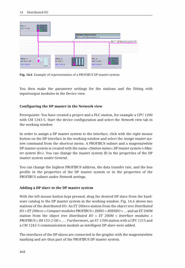
14 Distributed I/O
468
You then make the parameter settings for the stations and the fitting withinput/output modules in the Device view.
Configuring the DP master in the Network view
Prerequisite: You have created a project and a PLC station, for example a CPU 1200with CM 1243-5. Start the device configuration and select the Network view tab inthe working window.
In order to assign a DP master system to the interface, click with the right mousebutton on the DP interface in the working window and select the Assign master sys-tem command from the shortcut menu. A PROFIBUS subnet and a magenta/whiteDP master system is created with the name <Station name>.DP master system (<Mas-ter system ID>). You can change the master system ID in the properties of the DPmaster system under General.
You can change the highest PROFIBUS address, the data transfer rate, and the busprofile in the properties of the DP master system or in the properties of thePROFIBUS subnet under Network settings.
Adding a DP slave to the DP master system
With the left mouse button kept pressed, drag the desired DP slave from the hard-ware catalog to the DP master system in the working window. Fig. 14.6 shows twostations of the distributed I/O: An ET 200eco station from the object tree DistributedI/O > ET 200eco > Compact modules PROFIBUS > DI/DO > 8DI/8DO > … and an ET 200Mstation from the object tree Distributed I/O > ET 200M > Interface modules >PROFIBUS > IM 153-2 OD > … . Furthermore, an S7-1200 station with a CPU 1215 anda CM 1242-5 communication module as intelligent DP slave were added.
The interfaces of the DP slaves are connected in the graphic with the magenta/whitemarking and are thus part of the PROFIBUS DP master system.
Fig. 14.6 Example of representation of a PROFIBUS DP master system

14.3 PROFIBUS DP
469
Configuring a compact or modular DP slave
With the DP slave selected, you can set its properties in the Device view. You fit amodular DP slave with the desired modules or submodules from the hardware cat-alog and then set their parameters.
You set the PROFIBUS address in the properties of the PROFIBUS interface. Further-more, it is possible in the Module parameters group and depending on the DP slaveand application to set, for example, the startup property Start up if preset configu-ration does not match actual configuration, the DP interrupt mode, or the handlingof options.
Coupling an intelligent DP slave to the PROFIBUS DP master system
You initially create an intelligent DP slave (“I-slave”) as a stand-alone PLC stationand then connect the DP interface of the I-slave to the DP master system. You canfind the I-slaves in the hardware catalog in the PLC folder. For STEP 7 Basic V11 SP2,this is a CPU 1200 with CM 1242-5. Press and hold the left mouse button to drag theCPU from the object tree PLC > SIMATIC S7-1200 > CPU > … and into the working win-dow. In the same way, add the CM 1242-5 module from the object tree PLC > SIMATICS7-1200 > Communication module > PROFIBUS > CM 1242-5 > … to the station.
You establish a connection to the existing subnet if you drag the DP interface of theDP slave to the DP interface of another device on the subnet with the left mouse but-ton pressed, for example to the DP interface of the DP master.
In the properties of the DP interface of the I-slave, the DP slave option under Oper-ating mode is already activated. Select the assigned DP master from the drop-downlist. The station is then added as DP slave to the PROFIBUS DP master system.
Configuring the user data interface
You configure the user data interface to the DP master in the module properties ofthe I-slave. Select the CM module in the working window, and in the inspectorwindow tab Properties in the group PROFIBUS interface, select the entry Operatingmode > I-slave communication.
Double-click on <Add new> in the Transfer areas table. A new transfer area is cre-ated. You can change the name in the Transfer area column. In the Transfer directioncolumn (), click on the arrow to set the type of transfer area (arrow to the right means input area, arrow to the left means output area from the viewpoint of theI-slave).
Now set the start address in the Slave address column and the length of the transferarea in the Length column. The transfer area has a maximum length of 64 bytes. Inthe Master address column, set the start address which the transfer area has fromthe viewpoint of the DP master. In the Consistency column you can select betweenUnit and Total length (Fig. 14.7).
In this manner you can configure further transfer areas. The configured transferareas are displayed in the I-slave communication properties group. If you click a
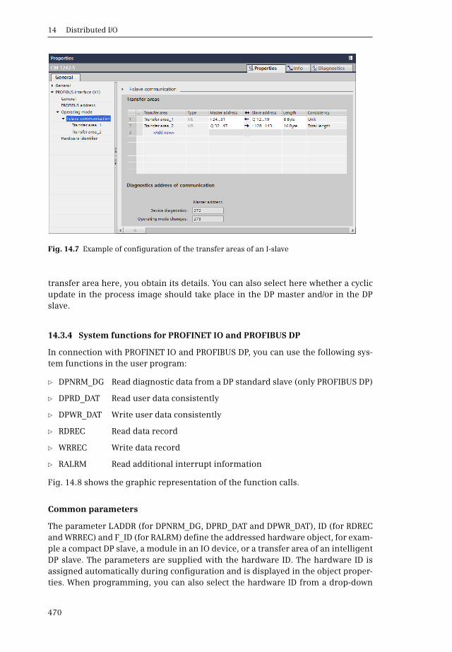
14 Distributed I/O
470
transfer area here, you obtain its details. You can also select here whether a cyclicupdate in the process image should take place in the DP master and/or in the DPslave.
14.3.4 System functions for PROFINET IO and PROFIBUS DP
In connection with PROFINET IO and PROFIBUS DP, you can use the following sys-tem functions in the user program:
b DPNRM_DG Read diagnostic data from a DP standard slave (only PROFIBUS DP)
b DPRD_DAT Read user data consistently
b DPWR_DAT Write user data consistently
b RDREC Read data record
b WRREC Write data record
b RALRM Read additional interrupt information
Fig. 14.8 shows the graphic representation of the function calls.
Common parameters
The parameter LADDR (for DPNRM_DG, DPRD_DAT and DPWR_DAT), ID (for RDRECand WRREC) and F_ID (for RALRM) define the addressed hardware object, for exam-ple a compact DP slave, a module in an IO device, or a transfer area of an intelligentDP slave. The parameters are supplied with the hardware ID. The hardware ID isassigned automatically during configuration and is displayed in the object proper-ties. When programming, you can also select the hardware ID from a drop-down
Fig. 14.7 Example of configuration of the transfer areas of an I-slave

14.3 PROFIBUS DP
471
menu: Double-click on the supply position in front of the parameter and select thedesired object from the drop-down menu, which contains all of the configured rel-evant objects.
Depending on the function, the RECORD parameter defines the source area fromwhich the data to be transferred is read, or the destination area into which thetransferred data are written. This can be a symbolically addressed tag or an abso-lutely addressed data area with the format P#[data block.]Operand Data type Num-ber (also see Chapter 4.2.3 “Absolute addressing of an operand area” on page 86).The source or destination area must be equal in length, as configured for theselected hardware object.
DPNRM_DG Read diagnostic data
DPNRM_DG reads the diagnostic data of a DP standard slave in the format specifiedin EN 50 170 Volume 2, PROFIBUS. The read procedure is triggered by REQ = “1” andis finished when BUSY signals “0”. The number of read bytes is then present in thefunction value RET_VAL. Depending on the slave, the diagnostic data is at least 6bytes and a maximum of 240 bytes long. The first 240 bytes are transferred if thediagnostic data is longer and then the corresponding overflow bit is set in the data.
The LADDR parameter is supplied with the hardware ID of the addressed object. TheRECORD parameter defines the area in which the read data is saved.
Note that DPMRM_DG is a system function which operates asynchronously. It mustbe processed until the BUSY parameter has signal state “0”. RALRM is a system
Fig. 14.8 Graphic representation of system blocks for PROFINET IO and PROFIBUS DP
Read data record
Write data record
Read diagnostic data from a standard slave
Read user data consistently
Write user data consistently
Read additional interrupt information
System blocks for PROFINET IO and PROFIBUS DP
14 Distributed I/O
472
block which makes the data available synchronously, i.e. immediately followingthe call.
DPRD_DAT Read user data consistently
DPRD_DAT reads consistent user data from a DP standard slave or IO device. ACPU 1200 supports 64 bytes of consistent data. Larger areas must be read withDPRD_DAT. This is optional for smaller areas. Areas read with DPRD_DAT must beremoved from the cyclic process image update.
The LADDR parameter is supplied with the hardware ID of the addressed object. TheRECORD parameter defines the area in which the read data is saved.
DPWR_DAT Write user data consistently
DPWR_DAT writes consistent user data to a DP standard slave or IO device. A CPU1200 supports 64 bytes of consistent data. Larger areas must be written withDPWR_DAT. This is optional for smaller areas. Areas written with DPRW_DAT mustbe removed from the cyclic process image update.
The LADDR parameter is supplied with the hardware ID of the addressed object. TheRECORD parameter defines the area from which the transferred data is read.
RDREC Read data record
RDREC reads a data record from a module. The ID parameter is supplied with thehardware ID of the addressed object. The RECORD parameter defines the area towhich the transferred data is written.
With signal state “1” at the REQ parameter, RDREC reads the data record INDEXfrom the module and saves it in the destination area RECORD. The MLEN parameterspecifies how many bytes are to be read. The assignment of INDEX and MLEN isdescribed in the manual of the respective module.
The transmission can be divided between several program cycles; the BUSY param-eter has signal state “1” during the transmission.
Signal state “1” in the VALID parameter signals that the data record has been readwithout errors. The LEN parameter then indicates the number of transferred bytes.In the event of an error, ERROR is set to “1”. Error information is then written to theSTATUS parameter.
WRREC Write data record
WRREC writes a data record to a module. The ID parameter is supplied with thehardware ID of the addressed object. The RECORD parameter defines the area fromwhich the data to be transferred is read.
With signal state “1” at the REQ parameter, WRREC writes the data record INDEXfrom the source area RECORD to the module. The LEN parameter specifies how
14.4 Actuator/sensor interface
473
many bytes are to be written. The assignment of INDEX and LEN is described in themanual of the respective module.
The transmission can be divided between several program cycles; the BUSY param-eter has signal state “1” during the transmission.
Signal state “1” in the DONE parameter signals that the data record has been writ-ten without errors. In the event of an error, ERROR is set to “1”. Error informationis then written to the STATUS parameter.
RALRM Read additional interrupt information
RALRM reads additional alarm information from an alarm-triggering hardwareobject on PROFINET IO or PROFIBUS DP, for example, from an IO device or a DPslave. It is called in the diagnostic interrupt organization block OB 82 or in a blockcalled within that block. Processing of RALRM is synchronous, i.e. the requesteddata is available at the output parameters immediately following the call.
The parameter F_ID is supplied with the hardware ID of the addressed object. Theassignment of the MODE parameter determines the mode of the system blockRALRM. With Mode = 0, RALRM shows you the interrupt-triggering component inthe ID parameter; signal state “1” is assigned to NEW. With Mode = 1, all outputparameters are written. With Mode = 2, RALRM checks whether the componentspecified by the F_ID parameter was the interrupt-triggering one. If this applies, theNEW parameter has signal state “1” and all other output parameters are written.
In bytes 0 to 19, the destination area TINFO (task information) contains the com-plete start information of the organization block in which RALRM was called, inde-pendent of the nesting depth in which it was called. Bytes 20 and 21 are filled withthe address of the hardware object. Bytes 22 to 31 contain management informa-tion, e.g. the ID number of the PROFINET IO device or the PROFIBUS DP slave.
The destination area AINFO (alarm information) contains the header informationand additional interrupt information. The header information for PROFIBUS DPoccupies bytes 0 to 3 and, for PROFINET IO, bytes 0 to 25 and contains, for example,the length of the received additional alarm information and the alarm type. Theadditional alarm information occupies bytes 4 to 223 (for PROFIBUS DP) and bytes26 to 1431 (for PROFINET IO) and is dependent upon the alarm type.
14.4 Actuator/sensor interface
14.4.1 Components of actuator/sensor interface
The actuator/sensor interface (AS-i) is an industrial fieldbus system for the lowestprocess level in automation plants in accordance with the open international stan-dard EN 50295. An AS-i master controls up to 62 AS-i slaves via a 2-wire AS-i cablethat transfers both the control signals and the supply voltage. Examples of mod-ules with AS-i master are the S7-1200 communication module CM 1243-2, the
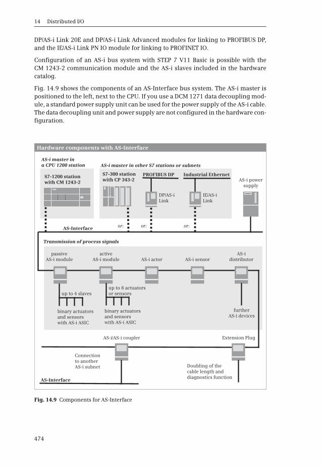
14 Distributed I/O
474
DP/AS-i Link 20E and DP/AS-i Link Advanced modules for linking to PROFIBUS DP,and the IE/AS-i Link PN IO module for linking to PROFINET IO.
Configuration of an AS-i bus system with STEP 7 V11 Basic is possible with theCM 1243-2 communication module and the AS-i slaves included in the hardwarecatalog.
Fig. 14.9 shows the components of an AS-Interface bus system. The AS-i master ispositioned to the left, next to the CPU. If you use a DCM 1271 data decoupling mod-ule, a standard power supply unit can be used for the power supply of the AS-i cable.The data decoupling unit and power supply are not configured in the hardware con-figuration.
Fig. 14.9 Components for AS-Interface
S7-1200 station with CM 1243-2 AS-i power
supply
AS-Interface
AS-Interface
Hardware components with AS-Interface
PROFIBUS DP Industrial Ethernet
Transmission of process signals
AS-i actor AS-i sensor
AS-i/AS-i coupler
AS-idistributor
Extension Plug
or: or: or:
DP/AS-iLink
IE/AS-iLink
binary actuators and sensors with AS-i ASIC
up to 4 slaves
passiveAS-i module
activeAS-i module
S
AS-i master in a CPU 1200 station AS-i master in other S7 stations or subnets
up to 8 actuators or sensors
binary actuators and sensors with AS-i ASIC
furtherAS-i devices
Connection to another AS-i subnet Doubling of the
cable length and diagnostics function
S7-300 station with CP 343-2
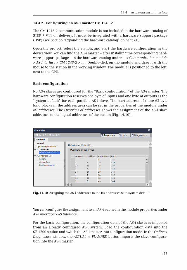
14.4 Actuator/sensor interface
475
14.4.2 Configuring an AS-i master CM 1243-2
The CM 1243-2 communication module is not included in the hardware catalog ofSTEP 7 V11 on delivery. It must be integrated with a hardware support package(HSP) (see Section “Expanding the hardware catalog” on page 60).
Open the project, select the station, and start the hardware configuration in thedevice view. You can find the AS-i master – after installing the corresponding hard-ware support package – in the hardware catalog under … > Communication module> AS Interface > CM 1243-2 > … . Double-click on the module and drag it with themouse to the station in the working window. The module is positioned to the left,next to the CPU.
Basic configuration
No AS-i slaves are configured for the “Basic configuration” of the AS-i master. Thehardware configuration reserves one byte of inputs and one byte of outputs as the“system default” for each possible AS-i slave. The start address of these 62-bytelong blocks in the address area can be set in the properties of the module underI/O addresses. The Overview of addresses shows the assignment of the AS-i slaveaddresses to the logical addresses of the station (Fig. 14.10).
You can configure the assignment to an AS-i subnet in the module properties underAS-i interface > AS Interface.
For the basic configuration, the configuration data of the AS-i slaves is importedfrom an already configured AS-i system. Load the configuration data into theS7-1200 station and switch the AS-i master into configuration mode. In the Online >Diagnostics window, the ACTUAL -> PLANNED button imports the slave configura-tion into the AS-i master.
Fig. 14.10 Assigning the AS-i addresses to the I/O addresses with system default
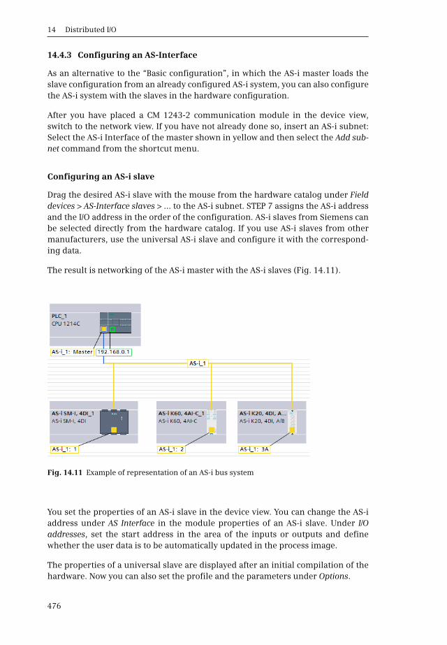
14 Distributed I/O
476
14.4.3 Configuring an AS-Interface
As an alternative to the “Basic configuration”, in which the AS-i master loads theslave configuration from an already configured AS-i system, you can also configurethe AS-i system with the slaves in the hardware configuration.
After you have placed a CM 1243-2 communication module in the device view,switch to the network view. If you have not already done so, insert an AS-i subnet:Select the AS-i Interface of the master shown in yellow and then select the Add sub-net command from the shortcut menu.
Configuring an AS-i slave
Drag the desired AS-i slave with the mouse from the hardware catalog under Fielddevices > AS-Interface slaves > … to the AS-i subnet. STEP 7 assigns the AS-i addressand the I/O address in the order of the configuration. AS-i slaves from Siemens canbe selected directly from the hardware catalog. If you use AS-i slaves from othermanufacturers, use the universal AS-i slave and configure it with the correspond-ing data.
The result is networking of the AS-i master with the AS-i slaves (Fig. 14.11).
You set the properties of an AS-i slave in the device view. You can change the AS-iaddress under AS Interface in the module properties of an AS-i slave. Under I/Oaddresses, set the start address in the area of the inputs or outputs and definewhether the user data is to be automatically updated in the process image.
The properties of a universal slave are displayed after an initial compilation of thehardware. Now you can also set the profile and the parameters under Options.
Fig. 14.11 Example of representation of an AS-i bus system

14.5 Communication via Modbus
477
14.4.4 Interface to user program
Access to AS-i slaves with binary values
You address the bits of an AS-i slave with binary scan or save functions. If you haveactivated the process image update in the configuration, the data is located in thearea of the inputs and outputs. If the process image update is deactivated, you mustaccess the slave data via the operand area Peripherals.
Access to AS-i slaves with analog values
If you have configured the AS-i slaves in the hardware configuration, you can accessthe analog values via the set I/O addresses. If the process image update has beenactivated in the configuration, the data is located in the area of the inputs and out-puts. If the process image update is deactivated, you must access the slave data viathe operand area Peripherals. As 16-bit value in a two's complement, the analogvalue occupies two byte addresses.
If the slave configuration has been imported from an already configured AS-i sys-tem, access the analog values with data records.
Access over the data record interface
To do this, use the system function RDREC for reading and WRREC for writing.RDREC and WRREC are described in the Chapter 14.3.4 “System functions forPROFINET IO and PROFIBUS DP” on page 470.
Calling up this function makes all of the functions of the M4 master profile of theAS-i master specification available. In the device manual of the CM 1243-2 commu-nication module, you can see which functions these are and how the parameters ofRDREC and WRREC must be assigned.
14.5 Communication via Modbus
Modbus is a standard protocol for data exchange between a “central” station (mas-ter/client) and several “distributed” stations (slaves/server). With Modbus RTU, thedata is transferred in binary-coded form, with Modbus TCP as TCP/IP packets. In aModbus network, a CPU 1200 can be both a master/client station and a slave/serverstation.
14.5.1 Modbus RTU
Modbus RTU (Remote Terminal Unit) utilizes serial data transmission with CM1241 RS232, CM 1241 RS485, or CB 1241 RS485. In the Modbus network (RTU), amaster station controls the data transfer and the slave stations receive or providethe data. In both stations, the communication function MB_COMM_LOAD config-ures the connector (port) on the module or on the board. In the master station, theMB_MASTER function controls the data transfer. In the slave station, the MB_SLAVEfunction controls the data transfer (Fig. 14.12).

14 Distributed I/O
478
The following functions are available for Modbus RTU communication:
b MB_COMM_LOAD Configuration of a port for the Modbus RTU protocol
b MB_MASTER Control for the Modbus master
b MB_SLAVE Control for a Modbus slave
Fig. 14.13 shows the calls of the communication functions in LAD representation.STEP 7 Basic V11 provides Version 2 of the Modbus RTU functions. The functions ofthis version may not be used together with functions of Version 1, as provided bySTEP 7 Basic V10.5.
Fig. 14.12 Data structure for the Modbus protocol (RTU)
Fig. 14.13 Calling the Modbus RTU functions in LAD representation
Data structure for the MODBUS protocol (RTU)
PORT PORT
MB_ADDR MB_ADDR
MB_DB MB_DB
DATA_ADDR
DATA_LEN
DATA_PTR MB_HOLD_REG
RS485RS232
RS485RS232
CM 1241CB 1241
CM 1241CB 1241
Modbus master Modbus slave
Slave Slave
Slave datain themaster
Modbusholdingregister
MB_COMM_LOAD_DB MB_COMM_LOAD_DB
MB_MASTER_DB MB_SLAVE_DB
MB_COMM_LOAD MB_COMM_LOAD
MB_MASTER MB_SLAVE
Slave data
Calls of MODBUS functions (RTU)

14.5 Communication via Modbus
479
Parameterization of the port with MB_COMM_LOAD
MB_COMM_LOAD configures the port (the connection) at the CM module or at thecommunication board for the Modbus RTU protocol. Executing MB_COMM_LOAD isa prerequisite for using MB_MASTER or MB_SLAVE. MB_COMM_LOAD can be calledup in the start-up program, for example, in order to set the port properties.
A rising edge at the REQ parameter starts a new job. A successfully executed job isindicated with the signal state “1” at the DONE parameter. If an error occurs duringjob processing, the ERROR parameter is set to signal state “1” and an error numberis output at the STATUS parameter.
The instance data block of MB_MASTER is created at the parameter MB_DB or, in theslave station, the instance data block of MB_SLAVE is created.
Controlling data traffic with MB_MASTER
MB_MASTER is called as single instance in the main program. A rising edge at theREQ parameter starts a new job. While the job is running, the BUSY parameter hassignal state “1”. A successfully executed job is indicated with the signal state “1” atthe DONE parameter. If an error occurs during job processing, the ERROR parame-ter is set to signal state “1” and an error number is output at the STATUS parameter.The assigning of these control parameters is only valid for one cycle until the nextprocessing of MB_MASTER.
The address of the slave station is at parameter MB_ADDR. The type of job at theslave station is defined at the MODE parameter, e.g. read inputs or write outputs.The DATA_ADDR and DATA_LEN parameters define the data area in the slave to beread or written.
MB_MASTER uses the data buffer defined at the DATA_PTR parameter as a clipboardfor the data which is read from the Modbus slave or written to the Modbus slave.The data buffer can be in the bit memory address area or in a data block. The Opti-mized block access attribute must be deactivated for a data block.
Responding master requests with MB_SLAVE
MB_SLAVE is called as single instance in the main program. The address of the slavestation is at parameter MB_ADDR. If the Modbus master has written data, the NDRparameter has signal state “1”. If the Modbus master has read data, the parameterDR has signal state “1”. If an error occurs during job processing, the ERROR param-eter is set to signal state “1” and an error number is output at the STATUS parame-ter. The assigning of these control parameters is only valid for one cycle until thenext processing of MB_SLAVE.
The parameter MB_HOLD_REG points to the Modbus holding register, which is usedby the MB_SLAVE as a clipboard for the data that is read from the Modbus masteror is written to the Modbus master. The holding register can be in the bit memoryaddress area or in a data block. The Optimized block access attribute must be deac-tivated for a data block.
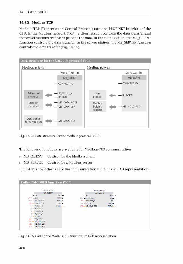
14 Distributed I/O
480
14.5.2 Modbus TCP
Modbus TCP (Transmission Control Protocol) uses the PROFINET interface of theCPU. In the Modbus network (TCP), a client station controls the data transfer andthe server stations receive or provide the data. In the client station, the MB_CLIENTfunction controls the data transfer. In the server station, the MB_SERVER functioncontrols the data transfer (Fig. 14.14).
The following functions are available for Modbus-TCP communication:
b MB_CLIENT Control for the Modbus client
b MB_SERVER Control for a Modbus server
Fig. 14.15 shows the calls of the communication functions in LAD representation.
Fig. 14.14 Data structure for the Modbus protocol (TCP)
Fig. 14.15 Calling the Modbus TCP functions in LAD representation
Data structure for the MODBUS protocol (TCP)
CONNECT_ID CONNECT_ID
IP_PORTIP_OCTET_x
IP_PORT
MB_DATA_ADDR
MB_DATA_LEN
MB_DATA_PTR
MB_HOLD_REG
Address ofthe server
Data onthe server
Modbus client Modbus server
Portnumber
Data bufferfor server data
MB_CLIENT_DB MB_SLAVE_DB
MB_CLIENT MB_SLAVE
Modbusholdingregister
Calls of MODBUS functions (TCP)
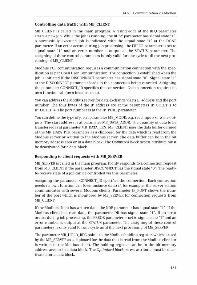
14.5 Communication via Modbus
481
Controlling data traffic with MB_CLIENT
MB_CLIENT is called in the main program. A rising edge at the REQ parameterstarts a new job. While the job is running, the BUSY parameter has signal state “1”.A successfully executed job is indicated with the signal state “1” at the DONEparameter. If an error occurs during job processing, the ERROR parameter is set tosignal state “1” and an error number is output at the STATUS parameter. Theassigning of these control parameters is only valid for one cycle until the next pro-cessing of MB_CLIENT.
Modbus TCP communication requires a communication connection with the spec-ification as per Open User Communication. The connection is established when thejob is initiated if the DISCONNECT parameter has signal state “0”. Signal state “1”at the DISCONNECT parameter leads to the connection being canceled. Assigningthe parameter CONNECT_ID specifies the connection. Each connection requires itsown function call (own instance data).
You can address the Modbus server for data exchange via its IP address and the portnumber. The four bytes of the IP address are at the parameters IP_OCTET_1 toIP_OCTET_4. The port number is at the IP_PORT parameter.
You can define the type of job at parameter MB_MODE, e.g. read inputs or write out-puts. The start address is at parameter MB_DATA_ADDR. The quantity of data to betransferred is at parameter MB_DATA_LEN. MB_CLIENT uses the data buffer definedat the MB_DATA_PTR parameter as a clipboard for the data which is read from theModbus server or written to the Modbus server. The data buffer can be in the bitmemory address area or in a data block. The Optimized block access attribute mustbe deactivated for a data block.
Responding to client requests with MB_SERVER
MB_SERVER is called in the main program. It only responds to a connection requestfrom MB_CLIENT if the parameter DISCONNECT has the signal state “0”. The ready-to-receive state of a job can be controlled via this parameter.
Assigning the parameter CONNECT_ID specifies the connection. Each connectionneeds its own function call (own instance data) if, for example, the server stationcommunicates with several Modbus clients. Parameter IP_PORT shows the num-ber of the port which is monitored by MB_SERVER for connection requests fromMB_CLIENT.
If the Modbus client has written data, the NDR parameter has signal state “1”. If theModbus client has read data, the parameter DR has signal state “1”. If an erroroccurs during job processing, the ERROR parameter is set to signal state “1” and anerror number is output at the STATUS parameter. The assigning of these controlparameters is only valid for one cycle until the next processing of MB_SERVER.
The parameter MB_HOLD_REG points to the Modbus holding register, which is usedby the MB_SERVER as a clipboard for the data that is read from the Modbus client oris written to the Modbus client. The holding register can be in the bit memoryaddress area or in a data block. The Optimized block access attribute must be deac-tivated for a data block.

15 Communication
482
15 Communication
15.1 Overview
Introduction to data communication with S7-1200
Communication is understood to be the data exchange between networked sta-tions. A station is a device containing a module with communication capability, forexample a programmable controller, an HMI device, or any other suitable third-party device. Communication is usually considered from the point of view of the“local” station connected with a partner station – the “remote” station. In the caseof a bus system, all stations are connected together over one single line; in the caseof a point-to-point connection, the connection is limited to two stations.
The physical connection on its own – the networking – is not sufficient for commu-nication. A specifically defined sequence, referred to as the protocol, is required toexchange the data. The communication partners and the protocol are defined whenestablishing a connection (“communication connection”).
A PLC station with a CPU 1200 can exchange data with other stations using variousmethods. The connection is made
b for Industrial Ethernet via the PROFINET interface on the CPU
b for PROFIBUS via the CM modules CM 1243-5 as DP master and CM 1242-5 as DP slave
b for AS-Interface via the CM module CM 1243-2 as AS-i master
b for point-to-point communication via a CM module CM 1241 or the communication board CB 1241
The communication with distributed I/O, for which the relevant “master module”that controls data traffic is inserted in the PLC station, is described in Chapter 14“Distributed I/O” on page 455.
An HMI station (of an HMI device) can be connected via Ethernet or PROFIBUS,depending on the device version. Data transmission requires a configured connec-tion (HMI connection). Special communication functions in the user program arenot required. The data exchange is defined during the configuration of the HMI sta-tion. Details can be found in Chapter 16 “Visualization” on page 507.
The communication between a PLC station and a programming device does notrequire any connection configuration or communication functions in the user pro-gram.

15.1 Overview
483
Data transmission via Industrial Ethernet
When configuring the networking and connections, Industrial Ethernet is handledlike a bus system. Strictly speaking, however, the Ethernet network consists only ofsingle point-to-point connections. If only two stations exchange data with eachother, they can be directly connected with a cable. If there are more than two sta-tions, a connection multiplier – such as the Compact Switch Module CSM 1277 – isneeded, which provides, for example, an interface with four ports. If a station hastwo ports connected with a switch, the bus cable can be guided to the next stationvia the second port. The configuration of each individual point-to-point connectionis necessary to calculate runtimes and response times.
Data transmission with open user communication
Open user communication transfers data between two PLC stations that are con-nected together via an Ethernet network. Data transmission can be secured withthe TCP and ISO-on-TCP protocols or unsecured with the UDP protocol. TCP andISO-on-TCP require a configured connection. The communication functionsTSEND_C for sending data and TRCV_C for receiving data form the interface to theuser program. The transmission with UDP is connectionless. The communicationaccess point is established in both stations with the TCON communication func-tion; it can then be used to send data (TUSEND) and receive data (TURCV).
Data transmission with S7 communication
S7 communication allows data to be transferred between two PLC stations con-nected via an Ethernet network or PROFIBUS. Data transmission requires a config-ured connection (“S7 connection”). The communication functions in the user pro-gram are GET to read data and PUT to write data. In the remote station, the CPUoperating system controls the data traffic without a communication function in theuser program.
Data transmission with a point-to-point connection
A PLC station with a CPU 1200 also supports a serial, character-based point-to-pointconnection. This type of communication allows a very generous definition of theprotocol. For example, a printer, barcode reader or modem can be connected to aCPU 1200 via a CM 1241 communication module using the RS232 or RS485 trans-mission standard.
The ASCII protocol is available for point-to-point communication, and – in globallibraries – the communication functions for MODBUS and USS drives.
Configuring communication with STEP 7 Basic
The networking and the connections are configured with the hardware configura-tion in the network view. The connection of a programming device is not configuredexcept for the parameterization of the PROFINET interface (IP address). Networkingwith a programming device and a connection multiplier as well as a point-to-pointconnection are not displayed in the network configuration.

15 Communication
484
In Fig. 15.1 you can see the networking (wiring) between the stations necessary fordata exchange. The lower part shows the configuration with the hardware configu-ration: In the networking view, the networking is represented by the Ethernet sub-net PN/IE_1 and in the connection view the configured connections between sta-tions are highlighted; in the example an HMI_Connection.
Before connecting to Ethernet, the PROFINET interface of the CPU must be param-eterized (see Section “IP address and subnet mask” on page 73). The connection ofa programming device is described in Chapter 13.1 “Connecting a programmingdevice to the PLC station” on page 421.
The PLC and HMI stations to be networked must be located together in one project.
15.2 Open user communication
15.2.1 Basics
Open user communication is a procedure for transmitting data between two sta-tions connected to the Ethernet subnet. Data exchange can be implemented usingthe protocols TCP in accordance with RFC 793, ISO-on-TCP in accordance with RFC1006, and UDP in accordance with RFC 768.
Fig. 15.1 Comparison of the wiring and configuration
Physical wiring of the stations
Representation with STEP 7 Basic in network view
Representation of networking
Representation of connection
CPU 1200 with CM
*)
CPU 1215 *)
HMI station
CSM 1277
Programming device
Barcode reader
S
PtP connection
A CPU 1215 has two connections which are connected to a switch and which allow a linear structure.

15.2 Open user communication
485
Data transmission with TCP and ISO-on-TCP is secure (with acknowledgment) overconfigured connections. Data transmission with UDP is unsecured (withoutacknowledgment) and connectionless.
Prerequisite for open user communication is the networking of the participatingstations via an Ethernet network. The (communication) connection is not createdwhen configuring the network with the connection table, but occurs via a data area.The communication functions at runtime use the address data in this data area toestablish the connection (for the TCP and ISO-on-TCP protocols) or to set up thecommunication access point (for UDP).
For open user communication with TCP or ISO-on-TCP, use the communicationfunctions TSEND_C and TRCV_C in the user program. These functions establish aconnection, control data traffic, and – depending on the programming – end theconnection. For the UDP protocol, the TCON communication function sets up theaccess point for the participating partner stations. The communication functionsTUSEND and TURCV control the data traffic, where dynamic addressing of theremote station at runtime is possible.
15.2.2 Open user communication with TCP and ISO-on-TCP
Data structure
Fig. 15.2 shows the data structure of open user communication with the use of theTCP and ISO-on-TCP protocols.
In the transmitting station, the communication function TSEND_C is called in theuser program. At the parameter CONNECT there is a pointer to a data block that hasthe structure of the system data type TCON_Param and contains the connectiondata. The parameter DATA points to the data to be sent. In the receiving station, thecommunication function TRCV_C is called in the user program. The parameterCONNECT is supplied with a data block that contains the connection data. Theparameter DATA contains a pointer to the receive mailbox in which the received datais stored.
Fig. 15.2 Communication functions TSEND_C and TRCV_C
Subnet
Industrial Ethernet
CPU 1200 CPU 1200
Reso
urc
es
CONNECT CONNECT
DATA DATA
Connectiondata
Transmissiondata
Connectiondata
Transmissiondata
TCON_Param TCON_ParamTSEND_C TRCV_C
Data transmission with TSEND_C and TRCV_C
Reso
urc
es

15 Communication
486
At runtime, the communication functions TSEND_C and TRCV_C establish a con-nection in both stations, transfer the data, and then – depending on the program-ming – end the connection.
As an alternative to TSEND_C and TRCV_C, the communications functions TCON,TDISCON, TSEND, and TRCV can be used. Fig. 15.3 shows the data structure usedhere.
Before a data transmission, a connection must be established in both stations withthe TCON communication function. At the parameter CONNECT there is a pointerto a data block that has the structure of the system data type TCON_Param and con-tains the connection data. The ID parameter identifies the communication connec-tion and must match the id tag in the connection data and the ID parameters of allcommunication functions involved in the connection.
In the transmitting station, the communication function TSEND is called in the userprogram. The parameter DATA points to the data to be sent. In the receiving station,the communication function TRCV is called in the user program. The parameterDATA contains a pointer to the receive mailbox in which the received data is stored.
With the communication function TDISCON, the connection can be terminated andthe connection resources released.
Transmission Control Protocol (TCP)
The transmission control protocol (TCP) is described in RFC 793. TCP is suitable formedium to large amounts of data (up to 8192 bytes) with static (fixed) data lengths.It is capable of routing. Performance features include, for example, recovery in caseof failure, flow control, and reliability.
Fig. 15.3 Communication functions TCON, TDISCON, TSEND, and TRCV
Subnet
Industrial Ethernet
CPU 1200 CPU 1200
CONNECT CONNECT
ID ID
ID ID
DATA DATA
ID ID
Connectiondata
Transmissiondata
Connectiondata
Transmissiondata
TCON_Param TCON_ParamTCON TCON
TDISCON TDISCON
TSEND TRCV
Data transmission with TCON, TDISCON, TSEND and TRCV
Con
nec
tion
res
ourc
es
Con
nec
tion
res
ourc
es

15.2 Open user communication
487
TCP is connection-oriented. Applications are addressed by means of port numbers.TCP is used if the communication partner does not support a connection usingISO-on-TCP. For such communication partners, enter “unspecified” as the partnerend point in the connection parameters.
If the number of sent bytes is smaller than the number of received bytes (controlledby the LEN parameters), the job is only signaled as being complete when the receivemailbox is full, i.e. the first bytes of the next job are also present in the receive mail-box. If the number of sent bytes is greater than the number of received bytes, thenumber of bytes specified in the LEN parameter are written into the receive mail-box, and the value of LEN is output in the RCVD_LEN parameter. The next block ofsent data is received with each further call.
ISO Transport over TCP (RFC 1006)
The RF 1006 protocol (ISO-on-TCP) can be used to import ISO applications into theTCP/IP network. It is suitable for medium to large quantities of data (up to8192 bytes) with dynamic lengths, is capable of routing, and use in a wireless net-work is possible.
Multiple connections can be established to a single IP address. The unambiguousassignment of a connection (communication endpoint) to an IP address is providedby a Transport Service Access Point (TSAP). You can define the TSAP for the connec-tion in the inspector window in the Configuration tab under Connection parameters.
If the number of sent bytes is smaller than the number of received bytes (controlledby the LEN parameters of both functions), the sent bytes are written into the receivemailbox, the job is signaled as being complete, and the RCVD_LEN parameter con-tains the number of received bytes. If the number of sent bytes is greater than thenumber of received bytes, no data is written into the receive mailbox, and the errorDestination buffer too small (status = 16#8088) is signaled.
15.2.3 Open user communication with the UDP protocol
Data structure
Fig. 15.4 shows the data structure of the open user communication with the use ofthe User Datagram Protocol (UDP).
In the transmitting station, the TCON communication function is called in the userprogram; it sets up the communication access point in the CPU operating system.The ID parameter identifies the connection between the user program and the CPUoperating system. The specification must match the ID parameter of the communi-cation function TUSEND and the id tag in the connection data at the parameterCONNECT. At the parameter CONNECT there is a pointer to a data block that has thestructure of the system data type TCON_Param and contains the connection data.
The communication function TUSEND sends the data specified at the DATA param-eter to the partner station. At the ADDR parameter there is a pointer to a data areawith the structure of the system data type TADDR_Param, which contains the IPaddress and the port number of the partner station.

15 Communication
488
In the receiving station, the communication function TCON is also called in the userprogram. The ID parameter identifies the connection between the user programand the CPU operating system. The specification must match the ID parameter ofthe communication function TURCV and the id tag in the connection data at theparameter CONNECT. At the parameter CONNECT there is a pointer to a data blockthat has the structure of the system data type TCON_Param and contains the con-nection data.
TURCV receives data from the transmitting station and writes it to the receive mail-box specified at the DATA parameter. At the ADDR parameter there is a pointer to adata area with the structure of the system data type TADDR_Param, which containsthe IP address and the port number of the partner station.
After data transmission, the communication function TDISCON disconnects thecommunication connection specified at the ID parameter or dissolves the commu-nication access point and frees the resources.
User datagram protocol (UDP)
Data transmission with UDP is described in RFC 768. The protocol is suitable fortransmitting small to medium amounts of data (up to 2048 bytes) quickly, becauseit is close to the hardware. It is capable of routing. The delivery of the data is unse-cured and there is no feedback about its receipt. The communication partner isaddressed as connectionless via the IP address and a port.
The communication functions TUSEND and TURCV handle the interface to the userprogram. The communication access point must first be set up with TCON in boththe local and the remote station.
Fig. 15.4 Communication functions TUSEND and TURCV
Subnetz
Industrial Ethernet
CPU 1200 CPU 1200
CONNECT CONNECT
ID ID
ID ID
DATA
ADDR
DATA
ADDR
ID ID
Transmissiondata
Partneraddress
TCON_Param TCON_Param
TADDR_ParamTADDR_Param
TCON TCON
TDISCON TDISCON
TUSEND TURCV
Data transmission with TCON, TDISCON, TSEND and TRCV
Data forthe access
point
Transmissiondata
Partneraddress
Data forthe access
point
Con
nec
tion
res
ourc
es
Con
nec
tion
res
ourc
es
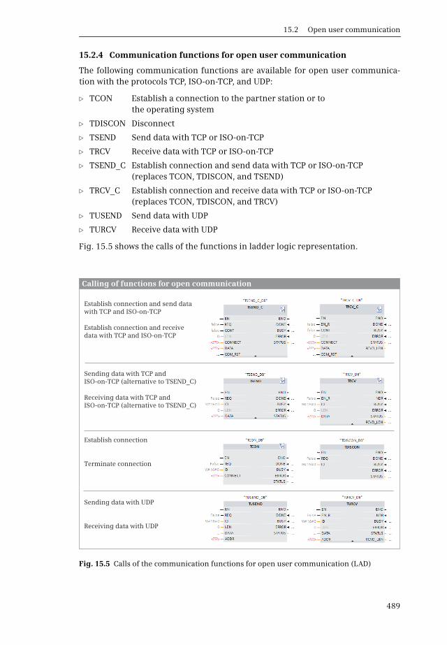
15.2 Open user communication
489
15.2.4 Communication functions for open user communication
The following communication functions are available for open user communica-tion with the protocols TCP, ISO-on-TCP, and UDP:
b TCON Establish a connection to the partner station or to the operating system
b TDISCON Disconnect
b TSEND Send data with TCP or ISO-on-TCP
b TRCV Receive data with TCP or ISO-on-TCP
b TSEND_C Establish connection and send data with TCP or ISO-on-TCP (replaces TCON, TDISCON, and TSEND)
b TRCV_C Establish connection and receive data with TCP or ISO-on-TCP (replaces TCON, TDISCON, and TRCV)
b TUSEND Send data with UDP
b TURCV Receive data with UDP
Fig. 15.5 shows the calls of the functions in ladder logic representation.
Fig. 15.5 Calls of the communication functions for open user communication (LAD)
Calling of functions for open communication
Establish connection
Terminate connection
Receiving data with UDP
Establish connection and send data with TCP and ISO-on-TCP
Establish connection and receive data with TCP and ISO-on-TCP
Sending data with TCP and ISO-on-TCP (alternative to TSEND_C)
Receiving data with TCP and ISO-on-TCP (alternative to TSEND_C)
Sending data with UDP

15 Communication
490
Description of common parameters
The communication functions for open user communication work asynchronously,i.e. job processing may require several program cycles under certain circumstanc-es. Use the REQ and EN_R parameters to control the data transmission The status ofdata transmission is shown by the BUSY, NDR, DONE, ERROR and STATUS parame-ters. You must evaluate these parameters immediately following each processing ofthe communication function since they are only valid up to the next call.
The CONT parameter with signal state “1” establishes a connection and retains it.Data transmission – the sending or receiving of data – only functions with the con-nection established. Signal state “0” on this parameter cancels the connectionagain.
If a rising signal edge occurs at parameter REQ, the task to send data starts. As longas the signal state is “1”, no other task for the specified connection is accepted. Onlywhen the communication function recognizes signal state “0” at REQ, can a newtask be started with the change to “1”.
The EN_R parameter activates data reception with signal state “1”. Data receipt isblocked if EN_R has the signal state “0”.
The DONE parameter shows with signal state “1” that the started job has been com-pleted without errors. It is only set for the duration of one program cycle.
The NDR parameter (New Data Ready) shows with signal state “1” that the startedjob has been completed without errors and that new data has been received. It isonly set for the duration of one program cycle.
The BUSY parameter shows with signal state “1” that job processing has not yetbeen completed and that a new job cannot be started.
The ERROR parameter shows with signal state “1” that the started job has been com-pleted with an error. It is only set for the duration of one program cycle.
The STATUS parameter contains intermediate states or error information.
b If DONE or NDR = “1”, STATUS is occupied by 16#0000.
b If ERROR = “1”, STATUS is occupied by error information.
b If none of these bits is set, STATUS may contain intermediate states which indicate the progress of the started job.
The following parameters specify the data transmission:
The ID parameter identifies the communication connection between the transmit-ting and receiving station, or for UDP the connection between the user programand the communication access point in the CPU operating system.
The CONNECT parameter points to a data block with the data structure of the sys-tem data type TCON_Param, which contains the description of the connectionparameters.
The DATA parameter contains the send or receive mailbox for the transferred data.The send and receive mailbox is a tag, e.g. an ARRAY tag in a data block, or an abso-

15.2 Open user communication
491
lutely addressed range, e.g. a range of 32 bytes in the data block DB 10 starting atbyte 64: P#DB10.DBX64.0 BYTE 32.
The ADDR parameter contains the IP address and the port number of the partnerstation with the data structure of the system data type ADDR_Param.
TSEND_C Establish connection and send data
The communication function TSEND_C establishes a connection, and sends datawith the TCP or ISO-on-TCP protocol. TSEND_C can also cancel the connectionagain.
Establishment of the connection is started if TSEND_C is processed with CONT = “1”.Following successful establishment, the DONE parameter is set to “1” for the dura-tion of one program cycle. Data is sent via an established connection when a risingedge occurs at the REQ parameter. Following successful transmission, DONE is setto “1” for the duration of one program cycle.
With CONT = “0” the connection is canceled immediately in both the send stationand the partner station.
If the COM_RST parameter has signal state “1”, TSEND_C is started again: an exist-ing connection is canceled, and a new one established.
The LEN parameter specifies the maximum number of bytes which are sent.
TRCV_C Establishing a connection and receiving data
The communication function TRCV_C establishes a connection, and receives datawith the TCP or ISO-on-TCP protocol. TRCV_C can also cancel the connection again.
Establishment of the connection is started if TRCV_C is processed with CONT = “1”.Following successful establishment, the DONE parameter is set to “1” for the dura-tion of one program cycle. TRCV_C only receives data when the EN_R parameter hassignal state “1”. Following successful receipt of data, the DONE parameter is set to“1” for the duration of one program cycle. Data is received continuously if CONT =“1” and EN_R = “1”.
With CONT = “0” the connection is canceled immediately in both the send stationand the partner station.
If the COM_RST parameter has signal state “1”, TRCV_C is started again: an existingconnection is canceled, and a new one established.
The parameter LEN specifies the number of bytes received. If LEN is filled with zero,as many bytes are received as contained in the tag at the DATA parameter. After suc-cessful data transmission, the parameter RCVD_LEN contains the number of bytesactually transmitted.
15 Communication
492
Data transmission with TCON, TDISCON, TSEND and TRCV
TCON establishes a communication connection to the partner device. The IDparameter identifies the connection. The specification must correspond to the idtag in the connection data at the parameter CONNECT.
The TSEND function sends data with the TCP or ISO-on-TCP protocol over an existingcommunication connection specified by the ID parameter. The DATA parametercontains a pointer to the send mailbox. You can use the LEN parameter to specifythe maximum number of bytes to be sent.
The TRCV function receives data with the TCP or ISO-on-TCP protocol over an exist-ing communication connection specified by the ID parameter. The DATA parametercontains a pointer to the receive mailbox. You can use the LEN parameter to specifythe number of bytes to be received. If LEN is “0”, the number of bytes received cor-responds to the tag at the DATA parameter. Following successful data transmission,the RCVD_LEN parameter contains the number of actually transmitted bytes.
TDISCON terminates the communication connection specified at the ID parameterand releases the connection resources.
TUSEND Send data with the UDP protocol
The TUSEND communication function sends data with the UDP protocol. A prereq-uisite is the previous establishment of a communication access point by TCON.
The assignment of the ID parameter designates the connection between the userprogram and the communication access point of the operating system. The valuemust agree with the id tag in the connection data. Specify the send mailbox with apointer at the DATA parameter.
The information on the communication partner is located in a data area to whichthe pointer at the ADDR parameter points. With each new send job, the address andthus the partner can be changed without having to redefine the communicationaccess point with TCON.
In the initial state, the REQ, BUSY, DONE, and ERROR parameters have signal state“0”. Start data transfer with a rising edge at the REQ parameter. On the initial callwith “1”, the data is fetched from the area specified by the DATA parameter. Thenumber of bytes specified at the LEN parameter is sent (1 to max. 1460).
While the job is running, BUSY = “1”. The job has been successfully completed ifBUSY = “0”, DONE = “1”, and ERROR = “0”. If the job contains errors, then BUSY =“0”, DONE = “0”, and ERROR = “1”. The error is then specified at the STATUS param-eter. BUSY, DONE, and ERROR are reset to “0” if REQ is returned to “0”.
The data in the send area can then be modified again when either DONE or ERRORhas signal state “1”.
15.2 Open user communication
493
TURCV Receive data with the UDP protocol
The communication function TURCV receives data with the UDP protocol. A prereq-uisite is the previous establishment of a communication access point by TCON.
The assignment of the ID parameter designates the connection between the userprogram and the communication access point of the operating system. The valuemust agree with the id tag in the connection data. Specify the receive mailbox witha pointer at the DATA parameter.
The information on the communication partner is located in a data area to whichthe pointer at the ADDR parameter points. The number of bytes to be received is setat the LEN parameter (1 to max. 1460). After a data block has been received, thenumber of bytes received is made available at the RCVD_LEN parameter and NDR isset to signal state “1”. Data is only received if the EN_R parameter has signal state“1”.
While the job is running, BUSY = “1”. The job has been successfully completed ifBUSY = “0”, NDR = “1”, and ERROR = “0”. If the job contains errors, BUSY = “0”, NDR= “0”, and ERROR = “1”. The error is then specified at the STATUS parameter. BUSY,NDR, and ERROR are reset to “0” if EN_R is returned to “0”.
The data in the receive area is consistent if NDR has signal state “1”.
15.2.5 Configuring open user communication
Prerequisite for open user communication is the networking of the PLC stationsparticipating in the data exchange via Industrial Ethernet. The required procedureis described in Chapter 3.4 “Configuring the network” on page 67. No connection isconfigured in the connection table for open user communication.
The communication functions for open user communication are called in the mainprogram, for example in a function block that is called in the organization block OB1 or another organization block with the event class Program cycle.
The communication functions can be found in the program elements catalog in thefolder Communication > Open user communication. Drag the desired communica-tion function into the opened block. When you release the mouse button, you willbe prompted to specify the call option. Select the Single instance option; a separatedata block is then assigned to the call.
In the inspector window under Properties in the Configuration tab, the program edi-tor shows the block parameters and also the connection parameters for the commu-nication functions TCON, TSEND_C, and TRCV_C (Fig. 15.6).
Fill out the fields highlighted in red that are still empty. If entries remain open,for example because the data areas still have to be created in the partner station,you will later be shown the connection dialog again if the communication functionis selected.
In the connection dialog, you specify the partner device, the connection type (TCPor ISO-on-TCP, for TCON also UDP), and the connection ID. The connection ID iden-

15 Communication
494
tifies the connection and must be the same in both stations. (Multiple connectionsbetween the partners can be created.)
In the Connection data field, specify the name of a data block, which is then createdby the program editor and parameterized at the CONNECT parameter. If you pro-gram the communication function appropriate to the connection in parallel in thepartner device, a data block with the connection data is also created here. Enter thisdata block in the Connection data field under Partner. The data block with the con-nection data is a type data block with the structure of the system data typeTCON_Param.
Use the Establish active connection option to specify which of the stations is to initi-ate the connection.
For the TCP and UDP connection types, enter the port number of the partner underAddress details. The number 2000 (dec) is specified by default. If you create multipleconnections, assign each connection its own port number (in the range of 2000 to5000 decimal).
For the connection type ISO-on-TCP, enter the access points (TSAP). The TSAP_IDmust be unique in a station. If you create multiple connections, assign each connec-tion its own TSAP ID. A TSAP has a length of 2 to 16 bytes.
By default, when configuring the connection editor, the TSAP “E0.01.49.53.4F.6F.6E.54.43.50.2D.31” is assigned. The first byte “E0” stands for open user communi-cation. “01” specifies the module (rack = 0, slot = 1). The next bytes are the ASCIIcharacters “ISOonTCP-1”.
Fig. 15.6 Configuring the connection parameters for open user communication
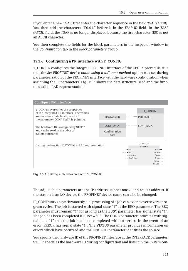
15.2 Open user communication
495
If you enter a new TSAP, first enter the character sequence in the field TSAP (ASCII).You then add the characters “E0.01.” before it in the TSAP ID field. In the TSAP(ASCII) field, the TSAP is no longer displayed because the first character (E0) is notan ASCII character.
You then complete the fields for the block parameters in the inspector window inthe Configuration tab in the Block parameters group.
15.2.6 Configuring a PN interface with T_CONFIG
T_CONFIG configures the integral PROFINET interface of the CPU. A prerequisite isthat the Set PROFINET device name using a different method option was set duringparameterization of the PROFINET interface with the hardware configuration whenassigning the IP parameters. Fig. 15.7 shows the data structure used and the func-tion call in LAD representation.
The adjustable parameters are the IP address, subnet mask, and router address. Ifthe station is an I/O device, the PROFINET device name can also be changed.
IP_CONF works asynchronously, i.e. processing of a job can extend over several pro-gram cycles. The job is started with signal state “1” at the REQ parameter. The REQparameter must remain “1” for as long as the BUSY parameter has signal state “1”.The job has been completed if BUSY = “0”. The DONE parameter indicates with sig-nal state “1” that the job has been completed without errors. In the event of anerror, ERROR has signal state “1”. The STATUS parameter provides information onerrors which have occurred and the ERR_LOC parameter identifies the source.
You specify the hardware ID of the PROFINET interface at the INTERFACE parameter.STEP 7 specifies the hardware ID during configuration and lists it in the System con-
Fig. 15.7 Setting a PN interface with T_CONFIG
CONF_DATA
INTERFACE
Configurationdata
Hardware ID
T_CONFIG
CONF_DATA
Configure PN interface
T_CONFIG overwrites the properties of the integrated PN interface. The values are saved in a data block, to which the parameter CONF_DATA is pointing.
The hardware ID is assigned by STEP 7 and can be read in the table of system constants.
Calling the function T_CONFIG in LAD representation
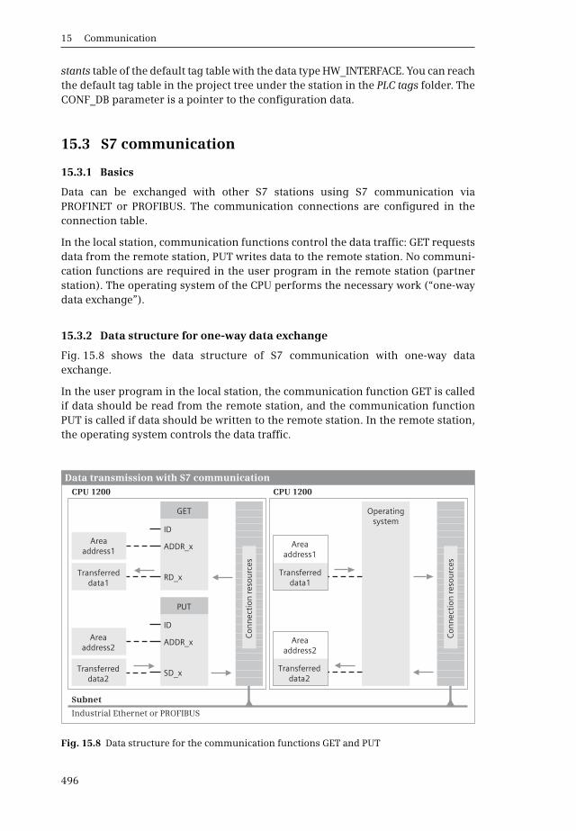
15 Communication
496
stants table of the default tag table with the data type HW_INTERFACE. You can reachthe default tag table in the project tree under the station in the PLC tags folder. TheCONF_DB parameter is a pointer to the configuration data.
15.3 S7 communication
15.3.1 Basics
Data can be exchanged with other S7 stations using S7 communication viaPROFINET or PROFIBUS. The communication connections are configured in theconnection table.
In the local station, communication functions control the data traffic: GET requestsdata from the remote station, PUT writes data to the remote station. No communi-cation functions are required in the user program in the remote station (partnerstation). The operating system of the CPU performs the necessary work (“one-waydata exchange”).
15.3.2 Data structure for one-way data exchange
Fig. 15.8 shows the data structure of S7 communication with one-way dataexchange.
In the user program in the local station, the communication function GET is calledif data should be read from the remote station, and the communication functionPUT is called if data should be written to the remote station. In the remote station,the operating system controls the data traffic.
Fig. 15.8 Data structure for the communication functions GET and PUT
Subnet
Industrial Ethernet or PROFIBUS
CPU 1200 CPU 1200
ADDR_x
ADDR_x
ID
ID
RD_x
SD_x
Areaaddress1
GET
PUT
Operatingsystem
Data transmission with S7 communication
Con
nec
tion
res
ourc
es
Con
nec
tion
res
ourc
es
Transferreddata1
Areaaddress2
Transferreddata2
Areaaddress1
Transferreddata1
Areaaddress2
Transferreddata2

15.3 S7 communication
497
At the parameters ADDR_1 to ADDR_4, you define the data areas in the remote sta-tion with absolute addressing. With the communication function GET you definethe receive mailboxes for the read data at the parameters RD_1 to RD_4. With thecommunication function PUT, you define the send mailboxes for the data to be writ-ten at the parameters SD_1 to SD_4.
No user program for sending or receiving is required in the remote station. Theremote station can transmit the data in the operating modes STOP and RUN.
15.3.3 Communication functions for one-way data exchange
The following blocks are available for one-way data exchange:
b GET Read data from a partner CPU
b PUT Write data to a partner CPU
GET and PUT have four send and receive areas that are shown when the represen-tation is opened. Fig. 15.9 shows the calls of the functions in ladder logic represen-tation.
Description of parameters
At the ID parameter, you specify the connection over which the data traffic is to beimplemented. Here you specify the connection ID from the connection table. Theconnection ID can be changed during runtime so that an instance data block can beused for several connections.
At the parameters ADDR_1 to ADDR_4 with the REMOTE data type, you define thedata areas in the remote station with absolute addressing. Example: The pointerP#DB24.DBX0.0 BYTE 32 defines an area of 32 bytes in data block DB 24 beginningwith data byte DB 0 (see also Chapter 4.2.3 “Absolute addressing of an operandarea” on page 86).
With the communication function GET you define the receive mailboxes for the readdata at the parameters RD_1 to RD_4: RD_1 for the data from the field ADDR_1, etc.With the communication function PUT, you define the send mailboxes for the datato be written at parameters SD_1 to SD_4, with SD_1 for the area ADDR_1, etc.
Fig. 15.9 Calls of the communication functions for S7 communication (LAD)
Read data with one-way data exchange
Write data with one-way data exchange
Calling of communication functions for S7 communication
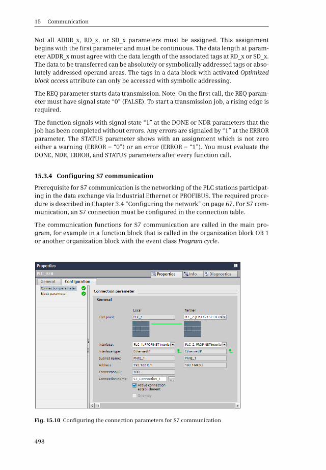
15 Communication
498
Not all ADDR_x, RD_x, or SD_x parameters must be assigned. This assignmentbegins with the first parameter and must be continuous. The data length at param-eter ADDR_x must agree with the data length of the associated tags at RD_x or SD_x.The data to be transferred can be absolutely or symbolically addressed tags or abso-lutely addressed operand areas. The tags in a data block with activated Optimizedblock access attribute can only be accessed with symbolic addressing.
The REQ parameter starts data transmission. Note: On the first call, the REQ param-eter must have signal state “0” (FALSE). To start a transmission job, a rising edge isrequired.
The function signals with signal state “1” at the DONE or NDR parameters that thejob has been completed without errors. Any errors are signaled by “1” at the ERRORparameter. The STATUS parameter shows with an assignment which is not zeroeither a warning (ERROR = “0”) or an error (ERROR = “1”). You must evaluate theDONE, NDR, ERROR, and STATUS parameters after every function call.
15.3.4 Configuring S7 communication
Prerequisite for S7 communication is the networking of the PLC stations participat-ing in the data exchange via Industrial Ethernet or PROFIBUS. The required proce-dure is described in Chapter 3.4 “Configuring the network” on page 67. For S7 com-munication, an S7 connection must be configured in the connection table.
The communication functions for S7 communication are called in the main pro-gram, for example in a function block that is called in the organization block OB 1or another organization block with the event class Program cycle.
Fig. 15.10 Configuring the connection parameters for S7 communication

15.4 Point-to-point communication
499
The communication functions can be found in the program elements catalog in thefolder Communication > S7 communication. Drag the desired communication func-tion into the opened block. When you release the mouse button, you will beprompted to specify the call option. Select the Single instance option; a separate datablock is then assigned to the call.
Under Properties in the Configuration tab in the inspector window, the program edi-tor shows the connection parameters and the block parameters (Fig. 15.10).
Fill out the fields highlighted in red that are still empty. If entries remain open,for example because the partner station still has to be created, you will later beshown the connection dialog again if the communication function is selected.
In the connection dialog, select the S7 connection for data transmission or create anew connection by clicking Connection overview (the button with three dots). Theconnection ID identifies the connection and must be the same in both stations.(Multiple connections between the partners can be created.)
Use the Active connection establishment option to specify which of the stations is toinitiate the connection.
You then complete the fields for the block parameters in the inspector window inthe Configuration tab in the Block parameters group or supply the block parametersdirectly at the function call in the working area.
15.4 Point-to-point communication
15.4.1 Introduction to point-to-point communication
Point-to-point (PtP) communication can be used to exchange data with external de-vices such as printers or barcode readers over a serial interface.
A CPU 1200 supports the Freeport protocol for character-based, serial communica-tion so that the data transmission protocol can be completely configured via theuser program. The scope of delivery of STEP 7 also includes functions for datatransmission with the USS Drive protocol and the protocols Modbus RTU Masterand Modbus RTU Slave.
The point-to-point communication is implemented with the CM 1241 communica-tion module (transmission media RS232 or RS485). On the CM 1241 module are theindicators
b Diagnostics LEDFlashes red after switching-on until the module is addressed (recognized) by the CPU. It then flashes green until the module has been parameterized. When ready for operation, the LED lights up green permanently.
b Send LEDLights up when data is sent to the connected device.
b Receive LEDLights up when data is received from the connected device.
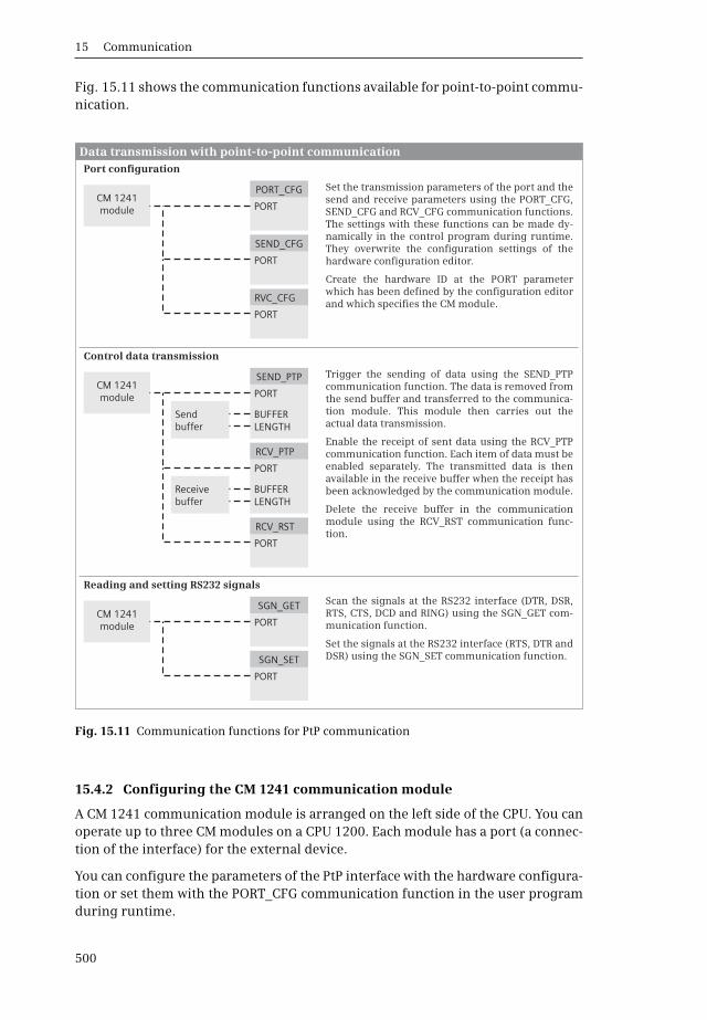
15 Communication
500
Fig. 15.11 shows the communication functions available for point-to-point commu-nication.
15.4.2 Configuring the CM 1241 communication module
A CM 1241 communication module is arranged on the left side of the CPU. You canoperate up to three CM modules on a CPU 1200. Each module has a port (a connec-tion of the interface) for the external device.
You can configure the parameters of the PtP interface with the hardware configura-tion or set them with the PORT_CFG communication function in the user programduring runtime.
Fig. 15.11 Communication functions for PtP communication
Port configuration
Reading and setting RS232 signals
PORT
PORT
PORT
PORT
PORT
Send buffer
Receive buffer
CM 1241module
CM 1241module
PORT_CFG
SGN_GET
SEND_CFG
SGN_SET
RVC_CFG
Data transmission with point-to-point communication
Control data transmission
PORT
BUFFER
BUFFER
LENGTH
LENGTH
PORT
PORT
CM 1241module
SEND_PTP
RCV_PTP
RCV_RST
Set the transmission parameters of the port and the send and receive parameters using the PORT_CFG, SEND_CFG and RCV_CFG communication functions. The settings with these functions can be made dy-namically in the control program during runtime. They overwrite the configuration settings of the hardware configuration editor.
Create the hardware ID at the PORT parameter which has been defined by the configuration editor and which specifies the CM module.
Trigger the sending of data using the SEND_PTP communication function. The data is removed from the send buffer and transferred to the communica-tion module. This module then carries out the actual data transmission.
Enable the receipt of sent data using the RCV_PTP communication function. Each item of data must be enabled separately. The transmitted data is then available in the receive buffer when the receipt has been acknowledged by the communication module.
Delete the receive buffer in the communication module using the RCV_RST communication func-tion.
Scan the signals at the RS232 interface (DTR, DSR, RTS, CTS, DCD and RING) using the SGN_GET com-munication function.
Set the signals at the RS232 interface (RTS, DTR and DSR) using the SGN_SET communication function.
15.4 Point-to-point communication
501
A prerequisite for configuring a communication module is a project with a PLC sta-tion. Start the device configuration editor in the project tree under the PLC station.In the device view, select the module on the Hardware Catalog task card – withactive filter function – under Communication modules > Point-to-point > and thedesired interface media (RS232, RS485, or RS422/485) and drag it to the slot on theleft of the CPU.
You can then set the configuration data in the inspection window.
Port configuration
With PtP communication, data is transmitted character-by-character. A charactercan consist of 7 or 8 bits. A parity bit can be transmitted in addition to the characterbits and is used for error detection: the signal state of the parity bit is selected foreven parity such that the total of the bits with signal state “1” is even, or odd withan odd parity. The transmitted character is terminated by 1 or 2 stop bits.
When you configure the ports, set the transmission rate (baud rate), the paritytype, number of data bits per character, and the number of stop bits.
Under Wait time you can select which time period to wait between transmissions.
You set the operating mode at the RS422/485 interface: Full duplex (simultaneoustransmission in both directions) or half duplex (transmission in only one directionat a time). In the multipoint-capable connection in full duplex operation, you canoperate the communication module as master or slave.
With the RS232 interface and the RS422/485 interface in full-duplex mode, youspecify under Flow control the method used to control the exchange of data betweensender and receiver. If you choose XON/XOFF, specify the encoding for the XON char-acter and the XOFF character.
Configuration of data transfer
It is possible to control the data traffic over the serial interface using a self-definedcommunication protocol. Set the transmission parameters depending on the RS232or RS485 standard under Configuration of transmitted message and then define thebeginning and end of the message under Configuration of received message.
15.4.3 Point-to-point communication functions
The following communication functions are available for PtP communication:
b PORT_CFG Set port configuration
b SEND_CFG Set send parameters
b RCV_CFG Set receive parameters
b SEND_PTP Trigger sending of data
b RCV_PTP Enable data receipt
b RCV_RST Empty receive buffer
b SGN_GET Read RS232 signals
b SGN_SET Write RS232 signals
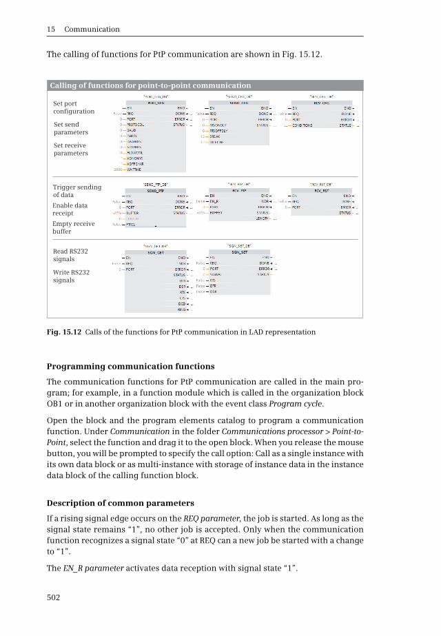
15 Communication
502
The calling of functions for PtP communication are shown in Fig. 15.12.
Programming communication functions
The communication functions for PtP communication are called in the main pro-gram; for example, in a function module which is called in the organization blockOB1 or in another organization block with the event class Program cycle.
Open the block and the program elements catalog to program a communicationfunction. Under Communication in the folder Communications processor > Point-to-Point, select the function and drag it to the open block. When you release the mousebutton, you will be prompted to specify the call option: Call as a single instance withits own data block or as multi-instance with storage of instance data in the instancedata block of the calling function block.
Description of common parameters
If a rising signal edge occurs on the REQ parameter, the job is started. As long as thesignal state remains “1”, no other job is accepted. Only when the communicationfunction recognizes a signal state “0” at REQ can a new job be started with a changeto “1”.
The EN_R parameter activates data reception with signal state “1”.
Fig. 15.12 Calls of the functions for PtP communication in LAD representation
Calling of functions for point-to-point communication
Set send parameters
Set receive parameters
Trigger sending of data
Enable data receipt
Empty receive buffer
Read RS232 signals
Write RS232 signals
Set port configuration

15.4 Point-to-point communication
503
The DONE parameter shows with signal state “1” that the started job has been com-pleted without errors. The parameter is only set for the duration of one programcycle.
The NDR parameter (New Data Ready) shows with signal state “1” that the startedjob has been completed without errors and that new data has been received. It isonly set for the duration of one program cycle.
The ERROR parameter shows with signal state “1” that the started job has been com-pleted with an error. It is only set for the duration of one program cycle.
The STATUS parameter contains intermediate states or error information:
b If DONE or NDR = “1”, STATUS is occupied by 16#0000.
b If ERROR = “1”, STATUS is occupied by error information.
b If none of these bits is set, STATUS may contain intermediate states which indicate the progress of the started job.
The following parameters specify the data transmission:
The PORT parameter specifies the CM module with the hardware ID which is definedwhen configuring the CM module.
The BUFFER and LENGTH parameters define the send or receive mailbox for thetransmitted data.
Changing the configuration settings during runtime
The properties of a port are set when configuring the CM module. These propertiesare “static”, which means they are transmitted from the load memory to theCM module when switching on the PLC station and apply to further operation. Us-ing communication functions, these properties can be changed “dynamically”during runtime. The “dynamically” changed properties are not permanent; theyare replaced by the “static” properties during the next call.
The PORT_CFG function changes the PORT properties such as baud rate, parity,number of data bits and stop bits.
The SEND_CFG function controls the intervals between activation of the RTS signaland start of data transmission, between the end of data transmission and deactiva-tion of the RTS signal, and the pauses at the beginnings and ends of messages.
The RCV_CFG function influences the conditions for the start and end of data to betransmitted. Data which satisfies these conditions can be received using theRCV_PTP communication function. The receive conditions are combined in the datastructure CONDITIONS.
Sending and receiving data
The SEND_PTP function transmits the data from the send mailbox in the user mem-ory to the CM module, and triggers the sending of data. The actual transmission tothe external device is handled by the CM module.
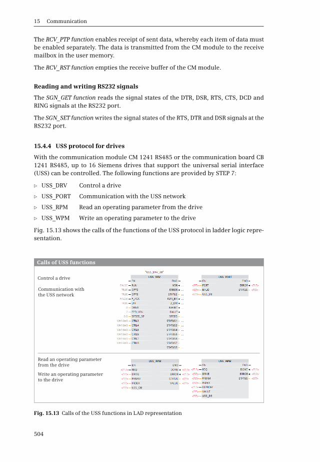
15 Communication
504
The RCV_PTP function enables receipt of sent data, whereby each item of data mustbe enabled separately. The data is transmitted from the CM module to the receivemailbox in the user memory.
The RCV_RST function empties the receive buffer of the CM module.
Reading and writing RS232 signals
The SGN_GET function reads the signal states of the DTR, DSR, RTS, CTS, DCD andRING signals at the RS232 port.
The SGN_SET function writes the signal states of the RTS, DTR and DSR signals at theRS232 port.
15.4.4 USS protocol for drives
With the communication module CM 1241 RS485 or the communication board CB1241 RS485, up to 16 Siemens drives that support the universal serial interface(USS) can be controlled. The following functions are provided by STEP 7:
b USS_DRV Control a drive
b USS_PORT Communication with the USS network
b USS_RPM Read an operating parameter from the drive
b USS_WPM Write an operating parameter to the drive
Fig. 15.13 shows the calls of the functions of the USS protocol in ladder logic repre-sentation.
Fig. 15.13 Calls of the USS functions in LAD representation
Calls of USS functions
Control a drive
Communication with the USS network
Read an operating parameter from the drive
Write an operating parameter to the drive

15.4 Point-to-point communication
505
A single data block is available for all controlled drives per CM 1241 communicationmodule or CB 1241 communication board. The transmission of data is taken overby the block USS_PORT. The block USS_DRV controls a drive whose number is spec-ified at the DRIVE parameter. The block USS_RPM reads an operating parameterfrom the drive; the block USS_WPM writes an operating parameter to the drive(Fig. 15.14).
The USS_DRV function block controls a drive. A separate call of the function block isrequired for each drive. You specify the drive number at the DRIVE parameter.When calling for the first drive, assign an instance data block to the function block.For all future calls, select the same data block as instance data block, which youchoose from a drop-down list.
The USS_RPM function reads an operating parameter from the drive whose numberyou specify at the DRIVE parameter. At the parameter USS_DB, the data block isspecified that contains the data for all drives of a CM module.
The USS_WPM function writes an operating parameter to the drive whose numberyou specify at the DRIVE parameter. At the parameter USS_DB, the data block isspecified that contains the data for all drives of a CM module. If you want to writethe parameter to the EEPROM of the drive control, take note of the limited numberof write accesses for an EEPROM.
Fig. 15.14 Data structure for the USS protocol
Data structure for the USS protocol
A data block contains the data of a module or of a board for all drives.
USS_DRV_DB
...DRIVE
USS_DB
USS_DB
USS_DB
DRIVE
DRIVE
RS485
CM 1241CB 1241
USS_DRV_DB
USS_DRV
USS_RPM
USS_WPM
USS_PORT
Common data
Data for Drive 1
Data for Drive 2
Data for Drive 3
...
Data for Drive 16
Drive 16
Drive 15
Drive 14
Drive 13
Drive 1
The USS protocol is used to control up to 16 drives with one CM 1241 RS485 module or a CB 1241 RS485 board.

15 Communication
506
The USS_PORT function transfers the drive data between the data block and the CMmodule. It is called only once per CM module.
The blocks USS_DRV, USS_RPM, and USS_WPM must be called in the main program;any organization block is possible for the block USS_PORT. The processing ofUSS_PORT must not be interrupted. The block must be called in a time interval thatdepends on the baud rate of the serial connection and the time response of thedrive.

16.1 Introduction to visualization
507
16 Visualization
16.1 Introduction to visualization
An HMI station (HMI = Human Machine Interface) is an operator control and mon-itoring device for manually controlling a process, for recording process data, andfor displaying process alarms.
The configuration data of the HMI station is saved in a “project”. A project containsall of the data for an automation solution. The project also includes the configura-tion data for a PLC station, since an HMI station on its own cannot control a process(machine or plant). The HMI station receives the data to be displayed from the pro-cess via the PLC station and controls the process via the PLC station. It is recom-mendable to generate the user program for the PLC station prior to configuring theHMI station; at least, however, the interface between the stations so that dataexchange can be configured at the HMI station end. The interface between the sta-tions comprises a logical connection which defines the type of data exchange (the
Fig. 16.1 Interface between HMI and PLC station
HMI connection
HMI station PLC station
Ethernet
PN/IE subnet
PLC tagsExternal HMI tags
Data blocksArea pointers
Interface between HMI and PLC station
The “Devices & networks” editor can be used to establish an HMI connection between the PLC and HMI station.
When defining the external HMI tags and area pointers, specify the HMI connection via which the data exchange is to take place and the corresponding tags in the PLC station. The external HMI tags and the area pointers in the HMI station are mapped 1:1 in the PLC station. Data exchange is carried out automatically by the HMI station at the intervals defined in the configuration.
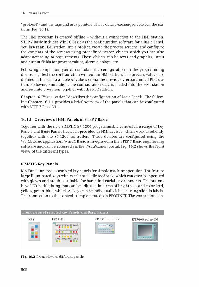
16 Visualization
508
“protocol”) and the tags and area pointers whose data is exchanged between the sta-tions (Fig. 16.1).
The HMI program is created offline – without a connection to the HMI station.STEP 7 Basic includes WinCC Basic as the configuration software for a Basic Panel.You insert an HMI station into a project, create the process screens, and configurethe contents of the screens using predefined screen objects which you can alsoadapt according to requirements. These objects can be texts and graphics, inputand output fields for process values, alarm displays, etc.
Following completion, you can simulate the configuration on the programmingdevice, e.g. test the configuration without an HMI station. The process values aredefined either using a table of values or via the previously programmed PLC sta-tion. Following simulation, the configuration data is loaded into the HMI stationand put into operation together with the PLC station.
Chapter 16 “Visualization” describes the configuration of Basic Panels. The follow-ing Chapter 16.1.1 provides a brief overview of the panels that can be configuredwith STEP 7 Basic V11.
16.1.1 Overview of HMI Panels in STEP 7 Basic
Together with the new SIMATIC S7-1200 programmable controller, a range of KeyPanels and Basic Panels has been provided as HMI devices, which work excellentlytogether with the S7-1200 controllers. These devices are configured using theWinCC Basic application. WinCC Basic is integrated in the STEP 7 Basic engineeringsoftware and can be accessed via the Visualization portal. Fig. 16.2 shows the frontviews of the different types.
SIMATIC Key Panels
Key Panels are pre-assembled key panels for simple machine operation. The featurelarge illuminated keys with excellent tactile feedback, which can even be operatedwith gloves and are thus suitable for harsh industrial environments. The buttonshave LED backlighting that can be adjusted in terms of brightness and color (red,yellow, green, blue, white). All keys can be individually labeled using slide-in labels.The connection to the control is implemented via PROFINET. The connection con-
Fig. 16.2 Front views of different panels
KP300 mono PNKP8 PP17-II KTP600 color PN
Front views of selected Key Panels and Basic Panels
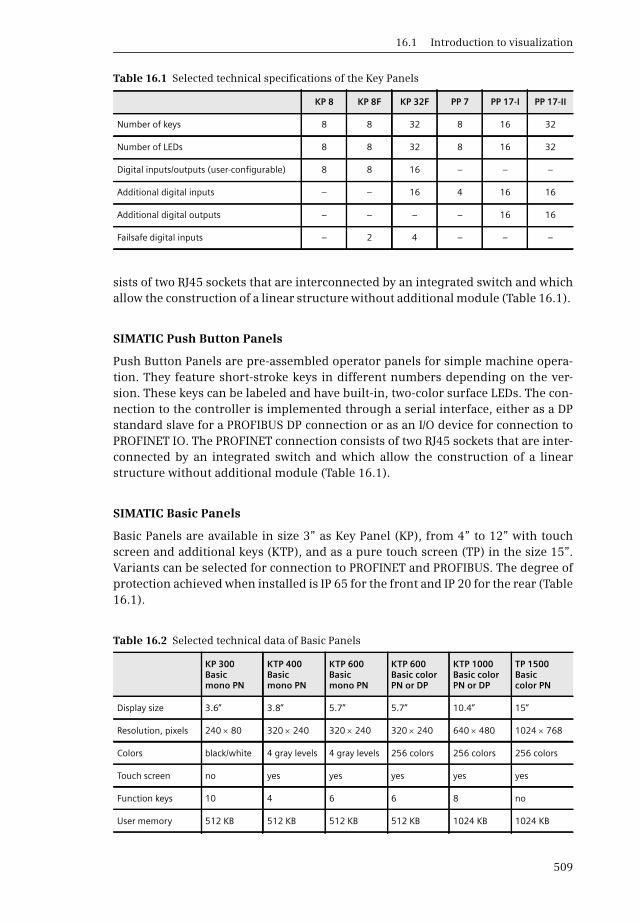
16.1 Introduction to visualization
509
sists of two RJ45 sockets that are interconnected by an integrated switch and whichallow the construction of a linear structure without additional module (Table 16.1).
SIMATIC Push Button Panels
Push Button Panels are pre-assembled operator panels for simple machine opera-tion. They feature short-stroke keys in different numbers depending on the ver-sion. These keys can be labeled and have built-in, two-color surface LEDs. The con-nection to the controller is implemented through a serial interface, either as a DPstandard slave for a PROFIBUS DP connection or as an I/O device for connection toPROFINET IO. The PROFINET connection consists of two RJ45 sockets that are inter-connected by an integrated switch and which allow the construction of a linearstructure without additional module (Table 16.1).
SIMATIC Basic Panels
Basic Panels are available in size 3” as Key Panel (KP), from 4” to 12” with touchscreen and additional keys (KTP), and as a pure touch screen (TP) in the size 15”.Variants can be selected for connection to PROFINET and PROFIBUS. The degree ofprotection achieved when installed is IP 65 for the front and IP 20 for the rear (Table16.1).
Table 16.1 Selected technical specifications of the Key Panels
KP 8 KP 8F KP 32F PP 7 PP 17-I PP 17-II
Number of keys 8 8 32 8 16 32
Number of LEDs 8 8 32 8 16 32
Digital inputs/outputs (user-configurable) 8 8 16 – – –
Additional digital inputs – – 16 4 16 16
Additional digital outputs – – – – 16 16
Failsafe digital inputs – 2 4 – – –
Table 16.2 Selected technical data of Basic Panels
KP 300 Basic mono PN
KTP 400 Basicmono PN
KTP 600 Basicmono PN
KTP 600 Basic color PN or DP
KTP 1000 Basic color PN or DP
TP 1500 Basiccolor PN
Display size 3.6” 3.8” 5.7” 5.7” 10.4” 15”
Resolution, pixels 240 80 320 240 320 240 320 240 640 480 1024 768
Colors black/white 4 gray levels 4 gray levels 256 colors 256 colors 256 colors
Touch screen no yes yes yes yes yes
Function keys 10 4 6 6 8 no
User memory 512 KB 512 KB 512 KB 512 KB 1024 KB 1024 KB
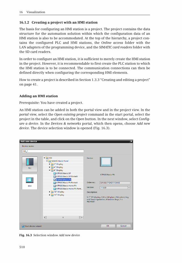
16 Visualization
510
16.1.2 Creating a project with an HMI station
The basis for configuring an HMI station is a project. The project contains the datastructure for the automation solution within which the configuration data of anHMI station is also to be accommodated. At the top of the hierarchy, a project con-tains the configured PLC and HMI stations, the Online access folder with theLAN adapters of the programming device, and the SIMATIC card readers folder withthe SD card readers.
In order to configure an HMI station, it is sufficient to merely create the HMI stationin the project. However, it is recommendable to first create the PLC station to whichthe HMI station is to be connected. The communication connections can then bedefined directly when configuring the corresponding HMI elements.
How to create a project is described in Section 1.3.3 “Creating and editing a project”on page 41.
Adding an HMI station
Prerequisite: You have created a project.
An HMI station can be added in both the portal view and in the project view. In theportal view, select the Open existing project command in the start portal, select theproject in the table, and click on the Open button. In the next window, select Config-ure a device. In the Devices & networks portal, which then opens, choose Add newdevice. The device selection window is opened (Fig. 16.3).
Fig. 16.3 Selection window Add new device

16.1 Introduction to visualization
511
To add an HMI station in the project view, open the project and double-click in theproject tree on the Add new device command. The device selection window is thenopened.
In the selection window, click on the “HMI” button, select the desired device fromthe hardware catalog, and assign a meaningful name. If you wish to be guided bythe HMI device wizard through the further basic configuration, activate the Startdevice wizard check box. Click on the OK button. The HMI device wizard is now start-ed if it has been activated, otherwise the HMI editor starts.
Using the HMI device wizard
The HMI device wizard guides you through the basic configuration in the followingsteps:
b In the PLC connections window you can select – if present – the PLC station to which the HMI station is to be connected.
b In the Screen layout window you can select the screen resolution and back-ground color and define whether a header is to be displayed with the date and company logo. The settings are stored in Template_1.
b In the Alarms window, you can select the alarms to be displayed: unacknowl-edged alarms, active alarms, and active system events. The settings are stored in Template_1.
Fig. 16.4 Configuring system screens using the HMI device wizard
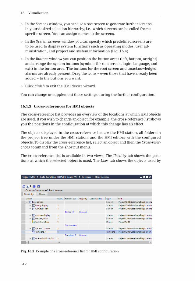
16 Visualization
512
b In the Screens window, you can use a root screen to generate further screens in your desired selection hierarchy, i.e. which screens can be called from a specific screen. You can assign names to the screens.
b In the System screens window you can specify which predefined screens are to be used to display system functions such as operating modes, user ad-ministration, and project and system information (Fig. 16.4).
b In the Buttons window you can position the button areas (left, bottom, or right) and arrange the system buttons (symbols for root screen, login, language, and exit) in the button area. The buttons for the root screen and unacknowledged alarms are already present. Drag the icons – even those that have already been added – to the buttons you want.
b Click Finish to exit the HMI device wizard.
You can change or supplement these settings during the further configuration.
16.1.3 Cross-references for HMI objects
The cross-reference list provides an overview of the locations at which HMI objectsare used. If you wish to change an object, for example, the cross-reference list showsyou the positions in the configuration at which this change has an effect.
The objects displayed in the cross-reference list are the HMI station, all folders inthe project tree under the HMI station, and the HMI editors with the configuredobjects. To display the cross-reference list, select an object and then the Cross-refer-ences command from the shortcut menu.
The cross-reference list is available in two views: The Used by tab shows the posi-tions at which the selected object is used. The Uses tab shows the objects used by
Fig. 16.5 Example of a cross-reference list for HMI configuration
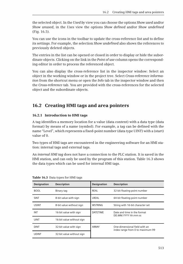
16.2 Creating HMI tags and area pointers
513
the selected object. In the Used by view you can choose the options Show used and/orShow unused, in the Uses view the options Show defined and/or Show undefined(Fig. 16.5).
You can use the icons in the toolbar to update the cross-reference list and to defineits settings. For example, the selection Show undefined also shows the references topreviously deleted objects.
The entries in the list can be opened or closed in order to display or hide the subor-dinate objects. Clicking on the link in the Point of use column opens the correspond-ing editor in order to process the referenced object.
You can also display the cross-reference list in the inspector window: Select anobject in the working window or in the project tree. Select Cross-reference informa-tion from the shortcut menu or open the Info tab in the inspector window and thenthe Cross-reference tab. You are provided with the cross-references for the selectedobject and the subordinate objects.
16.2 Creating HMI tags and area pointers
16.2.1 Introduction to HMI tags
A tag identifies a memory location for a value (data content) with a data type (dataformat) by means of a name (symbol). For example, a tag can be defined with thename “Level”, which represents a fixed-point number (data type UINT) with a (start)value of 0.
Two types of HMI tags are encountered in the engineering software for an HMI sta-tion: internal tags and external tags.
An internal HMI tag does not have a connection to the PLC station. It is saved in theHMI station, and can only be used by the program of this station. Table 16.3 showsthe data types which can be used for internal HMI tags.
Table 16.3 Data types for HMI tags
Designation Description Designation Description
BOOL Binary tag REAL 32-bit floating-point number
SINT 8-bit value with sign LREAL 64-bit floating-point number
USINT 8-bit value without sign WSTRING String with 16-bit character set
INT 16-bit value with sign DATETIME Date and time in the formatDD.MM.YYYY hh:mm:ss
UINT 16-bit value without sign
DINT 32-bit value with sign ARRAY One-dimensional field with an index range from 0 to maximum 99
UDINT 32-bit value without sign

16 Visualization
514
An external HMI tag (process tag) is the image of a memory location in the PLC sta-tion. This memory location can be accessed by both the HMI station – with the HMItag name – and by the PLC station – with the PLC tag name. If an HMI connectionbetween the PLC station and the HMI station is configured in network view, this iscalled an integrated connection. In an integrated connection, the PLC tag can beaddressed absolutely or symbolically and can be in a data block with optimizedaccess or standard access. A connection is not integrated if it is configured in theconnection table, for example because both stations are not located together in thesame project. A PLC tag can be accessed via a non-integrated connection only withabsolute addressing.
With the HMI configuration, the expression “PLC tag” stands for a tag in the PLC sta-tion. This can be a tag from the PLC tag table or a data tag from a data block.
The external HMI tags accept the data types assigned to them in the PLC station(PLC data types, not with data type STRUCT). With a PLC tag with data type ARRAY,the HMI tag accepts the number (“array elements”) and the data type of the ele-ments.
In addition to the external tags, it is also possible to exchange data between the HMIand PLC station using Area pointers.
16.2.2 Creating an HMI tag
All HMI tags are located in the project tree under the HMI station in the HMI tagsfolder. When creating an HMI station, the default tag table, into which you can enterthe HMI tags, is automatically created. Double-click on Add new tag table to addadditional tag tables. For the selected HMI tags folder, you can create subfolders fora better overview with the Add group command from the shortcut menu. A tag canonly be defined once (in an HMI station there is only a single tag table, which canbe divided into subtables). Double-click on Show all tags to obtain an overview of allconfigured HMI tags.
To create an HMI tag, open an HMI tag table by double-clicking on it. If you want tocreate an internal tag, select <Internal tag> as connection. In the Data type column,select the HMI data type from a drop-down list. For the ARRAY data type, enter therange in square brackets, followed by the keyword OF and the data type, e.g. ARRAY[0..24] OF INT.
With an external tag (process tag), set the connection to the PLC station and selectthe PLC tag. You can select tags from a PLC tag table or from data blocks (in the Pro-gram blocks) folder. The data type of the PLC tag is automatically applied. UnderAcquisition cycle, set the time interval with which the updating is to be carried out.Make sure with these settings that the communication load on the connectionbetween the HMI and PLC stations remains within acceptable limits.
16.2 Creating HMI tags and area pointers
515
Configuring an HMI tag
In the Properties tab of the inspector window, you can set further properties of theselected tag. For example, you can set the type of recording in the Properties sectionunder Settings:
b Cyclic in operation = the tag is updated regularly as long as it is displayed in a screen
b Cyclic continuous = the tag is updated regularly even if it is not displayed in a screen
b On demand = the tag is updated on request, e.g. by a system function
Under Range you can set an upper and a lower limit value for the selected tag. UnderLinear scaling the range of values of the PLC tag is converted linearly into a range ofvalues in the HMI station. Scaling is carried out for the data exchange in both direc-tions. The start value when switching on the HMI station or up to the first update isdefined under Values. Multiplexing (indirect addressing) allows you to determinethe used tag during runtime, and not before. A multiplex tag consisting of a list oftags is used for configuration. An index tag then selects the used tag from this list.
In the Events tab you can assign a function list with system functions to be executedif certain events such as a change in value or a limit violation occur.
16.2.3 Creating an area pointer
An area pointer defines a memory area in the PLC station. The programs of the HMIand PLC stations exchange data via this memory area. Example: when changing thescreen, the number of the current process screen is transferred to the PLC stationby means of the area pointer Screen number. The program of the PLC station can re-spond to this.
The area pointers must be configured prior to use. The length of an area pointer isspecified in 16-bit words. The memory area to which an area pointer refers is pres-ent in a data block in the user program. An area pointer with a length = 1 can alsobe a PLC tag from the PLC tag table. With a length of > 1, the PLC tag in the datablock is created with data type ARRAY and a 16-bit data type (e.g. WORD) with thelength of the area pointer, e.g. ARRAY [1..4] OF WORD.
Overview of area pointers
Table 16.4 lists the available area pointers. The global area pointers Screen number,Date/time PLC and Project ID can only be used once per station and only in one con-nection.
b Screen number: When changing the screen, the HMI station transfers the screennumber to the PLC station (global area pointer).
b Job mailbox: A control job consists of a job number and up to three parameters.The PLC station writes a control job into the data area; if the HMI station has ac-cepted the job, it overwrites the job number with zero.

16 Visualization
516
b Date/time: The PLC station writes the control job No. 41. The HMI station thentransfers the date and time in data type DTL to the PLC station.
b Date/time PLC: The PLC station writes the date and time in data type DTL to thedata area which is then read cyclically by the HMI station. The HMI station im-ports the date and time (global area pointer).
b Coordination: The HMI station transfers its actual operating mode in this data ar-ea: Startup (bit 0 = “0” during startup), offline/online mode (bit 1 = “0” with on-line mode) and communication readiness (by means of a “sign-of-life bit”, bit 2changes its signal state at approx. 1 Hz).
b Project ID: The HMI station can recognize whether it is connected to the “correct”PLC station. The project ID is created when configuring the HMI station: dou-ble-click on the Runtime settings editor in the project tree under the HMI station,and enter a value between 1 and 255 in the Screens section in the Project ID field.Then write the same value in the PLC station in the data area of the Project ID areapointer. During startup, the HMI station compares the two values, and does notstart unless they agree.
b Data record: The Data record area pointer is required for synchronized transferof a recipe data record. Handling of recipes is described in Section 16.4.3 “Work-ing with recipes” on page 535.
Table 16.4 Area pointers for Basic Panels
Area pointer Required for Length HMI PLC
Screen number Transfer of number of current screen 5 Writes Reads
Job mailbox Triggering of functions on the HMI station with the job numbers:14: Set time BCD-coded15: Set date BCD-coded23: Log on user24: Log off user40: Transfer date/time to PLC station41: Transfer date/time to PLC station (DTL)46: Update tag49: Clear event buffer50: Clear error alarm buffer51: Screen selection69: Read data record from PLC station70: Write data record to PLC station
4 Reads and
writes
Reads and
writes
Date/time Transfer of date and time to PLC station 6 Writes Reads
Date/time PLC Transfer of date and time to HMI station 6 Reads Writes
Coordination Transfer of HMI station status to PLC station 1 Writes Reads
Project ID Checking project ID in HMI station 1 Reads Writes
Data record Transfer of recipe data records with synchronization 5 Reads and
writes
Reads and
writes

16.3 Configuring process screens
517
Configuring an area pointer
Prerequisite: A PLC station, an HMI station, and an HMI connection have been cre-ated in the project. The user program of the PLC station contains a data block inwhich the data area for the area pointer is declared (see Chapter 6.4 “Programminga data block” on page 194).
Double-click on the Connections editor in the project tree under the HMI station.The top part of the connection window contains a table with the configured connec-tions.
There are two tables in the bottom part of the connection window in the Areapointers tab: the table with the area pointers created for the connection selected inthe connection table is shown at the top, and at the bottom the table with the globalarea pointers which can only be created once in the HMI station and only in one con-nection.
You can activate an area pointer in the top table using the Active check box and inthe bottom table by specifying the connection. Assign the PLC tag to the area point-er. The PLC tag must have been created previously in the PLC station with the samelength as the area pointer. You can set the acquisition cycle using the Job mailboxand Date/time PLC area pointers.
16.3 Configuring process screens
16.3.1 Introduction to configuring process screens
You use process screens to operate and monitor the process. A process screen canmap a plant, display process sequences, output process values, or facilitate opera-tor actions. Predefined objects are available for creating a screen, and can be insert-ed and adapted according to your requirements.
The properties of a screen, for example the resolution and colors, depend on theHMI station used.
A screen may consist of static and dynamic objects. Static objects are texts or graph-ics which do not change during process operation. Dynamic objects are e.g. texts,numerical values, trends and bars which change depending on process values.
You can also use a screen to access the process by means of control elements or tocall another screen. An input field allows definition of a setpoint for the process,and you can use function keys – if the HMI station is appropriately equipped – totrigger actions in the process, for example. Global function keys always trigger thesame action, regardless of the screen in which they are positioned. With local func-tion keys the triggered action depends on the displayed screen.
Configuration of the process screens is carried out in the following steps:
b Beginning with a root screen, the number of screens and their call hierarchy are defined.
b The navigation strategy within a screen and between screens is defined.

16 Visualization
518
b The existing template or the global screen is adapted, and/or new templates are created.
b Screens are created using the objects saved in the libraries.
16.3.2 Working window for process screens
The toolbar of the working window for process screens contains the most importantsetting options for the properties of a selected screen object or for displaying thescreen contents (Fig. 16.6).
Object properties such as the font family and color can also be set in the inspectorwindow. You can overlap objects, rotate them vertically and horizontally, and alignthem on the grid. You can set the grid width, grid display, and alignment on thegrid in the Grid section on the Layout task card.
You can use the zoom function to set the size – either using the icons in the toolbaror in the Zoom section on the Layout task card.
Fig. 16.6 Working window for process screens

16.3 Configuring process screens
519
16.3.3 Working with screen layers
Each process screen has 32 layers which are “overlaid”. Layer 0 is the lowest layer,layer 31 is in the foreground. Layers allow objects to be given nesting depth. Theobjects of a layer are also “stacked”. The first object inserted is located at the “rear”layer, the next one above it, etc. Objects can be shifted within a layer from the frontto the rear, or can be shifted to a different layer.
One of the 32 layers is always active; this is the layer at which the process screen iscurrently being processed. All 32 layers are displayed when a screen is opened.You can hide all layers during configuration except for the active layer.
You can set the visibility of a layer either with the selected screen background in theinspector window in the screen properties under Layers or on the Layout task cardunder Layers.
To change the (stack) sequence of an object, select the object and then one of theBring to front, Move forward, Move backward or Send to back commands from theOrder shortcut menu. The stack order of the objects present in the layer is alsoshown in the Layout task card: the highest object is the one at the rear. You can usethe mouse to drag the screen objects into a different order. In the same manner youcan drag a screen object to a different layer. You can also define the layer for ascreen object in the inspector window, in the screen properties under Miscella-neous.
16.3.4 Working with templates
You can use a (screen) template as the basis for a process screen. The screen thenimports the template's objects. You can modify these objects in the current screen,and add new objects. If you modify an object in the template, the object is modifiedin all screens based on this template.
The templates are saved in the project tree under the HMI station in the Screen man-agement folder under Templates. You can copy, rename or delete templates. You canstructure the Templates folder by selecting it and then the Add group command inthe shortcut menu.
A standard template is also created when you create an HMI station. You can adaptthis to your requirements: open the template in the project tree under the HMI proj-ect in the Screen management and Templates folder by double-clicking on Tem-plate_1. You can then add new objects or modify existing ones (see Section 16.3.8“Working with objects in process screens” on page 522).
You can also create other templates in addition to the standard template: double-click on Add new template in the Templates folder, and set the template's propertiesin the inspector window. You can then configure the contents of the template.
Global screen
In the global screen you can configure the screen objects for the entire HMI stationwhich then apply to all screens irrespective of the template on which they are
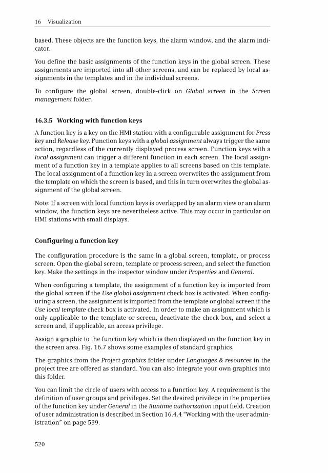
16 Visualization
520
based. These objects are the function keys, the alarm window, and the alarm indi-cator.
You define the basic assignments of the function keys in the global screen. Theseassignments are imported into all other screens, and can be replaced by local as-signments in the templates and in the individual screens.
To configure the global screen, double-click on Global screen in the Screenmanagement folder.
16.3.5 Working with function keys
A function key is a key on the HMI station with a configurable assignment for Presskey and Release key. Function keys with a global assignment always trigger the sameaction, regardless of the currently displayed process screen. Function keys with alocal assignment can trigger a different function in each screen. The local assign-ment of a function key in a template applies to all screens based on this template.The local assignment of a function key in a screen overwrites the assignment fromthe template on which the screen is based, and this in turn overwrites the global as-signment of the global screen.
Note: If a screen with local function keys is overlapped by an alarm view or an alarmwindow, the function keys are nevertheless active. This may occur in particular onHMI stations with small displays.
Configuring a function key
The configuration procedure is the same in a global screen, template, or processscreen. Open the global screen, template or process screen, and select the functionkey. Make the settings in the inspector window under Properties and General.
When configuring a template, the assignment of a function key is imported fromthe global screen if the Use global assignment check box is activated. When config-uring a screen, the assignment is imported from the template or global screen if theUse local template check box is activated. In order to make an assignment which isonly applicable to the template or screen, deactivate the check box, and select ascreen and, if applicable, an access privilege.
Assign a graphic to the function key which is then displayed on the function key inthe screen area. Fig. 16.7 shows some examples of standard graphics.
The graphics from the Project graphics folder under Languages & resources in theproject tree are offered as standard. You can also integrate your own graphics intothis folder.
You can limit the circle of users with access to a function key. A requirement is thedefinition of user groups and privileges. Set the desired privilege in the propertiesof the function key under General in the Runtime authorization input field. Creationof user administration is described in Section 16.4.4 “Working with the user admin-istration” on page 539.
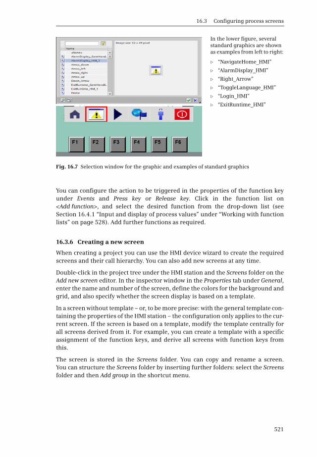
16.3 Configuring process screens
521
You can configure the action to be triggered in the properties of the function keyunder Events and Press key or Release key. Click in the function list on<Add function>, and select the desired function from the drop-down list (seeSection 16.4.1 “Input and display of process values” under “Working with functionlists” on page 528). Add further functions as required.
16.3.6 Creating a new screen
When creating a project you can use the HMI device wizard to create the requiredscreens and their call hierarchy. You can also add new screens at any time.
Double-click in the project tree under the HMI station and the Screens folder on theAdd new screen editor. In the inspector window in the Properties tab under General,enter the name and number of the screen, define the colors for the background andgrid, and also specify whether the screen display is based on a template.
In a screen without template – or, to be more precise: with the general template con-taining the properties of the HMI station – the configuration only applies to the cur-rent screen. If the screen is based on a template, modify the template centrally forall screens derived from it. For example, you can create a template with a specificassignment of the function keys, and derive all screens with function keys fromthis.
The screen is stored in the Screens folder. You can copy and rename a screen.You can structure the Screens folder by inserting further folders: select the Screensfolder and then Add group in the shortcut menu.
In the lower figure, several standard graphics are shown as examples from left to right:
b “NavigateHome_HMI”
b “AlarmDisplay_HMI”
b “Right_Arrow”
b “ToggleLanguage_HMI”
b “Login_HMI”
b “ExitRuntime_HMI”
Fig. 16.7 Selection window for the graphic and examples of standard graphics
16 Visualization
522
16.3.7 Configuring a screen change
Starting with a root screen which is displayed when the device is switched on, it ispossible to call further screens with a button or function key during runtime.The root screen, the further screens, and the links between the screens can be de-fined when creating the HMI project using the HMI device wizard. You can modifyor extend these definitions at any time.
To define the root screen, double-click in the project tree under the HMI station onRuntime settings and set the start screen in the General section.
Prerequisite for configuring a screen change: the screen to be selected is present inthe Screens folder, and the current screen is open in the working window.
In order to assign a screen change to a button, drag the screen to be opened into theworking window with the mouse button pressed. A button is created labeled withthe name of the screen. In order to assign a screen change to a function key, dragthe screen to be opened to the function key with the mouse button pressed.The function key then shows a yellow triangle.
You can then set the button's properties in the inspector window. Under Events andClick (with a button) or Events and Press key (with a function key) you can use theActivateScreen system function to set the new screen and the number of the objectwhich is to be focused following the screen change.
16.3.8 Working with objects in process screens
The graphic objects for designing process screens are present on the Tools taskcard (Table 16.5). When configuring screens and templates, Tools has the followingcategories:
b Basic objects (line, ellipse, circle, rectangle, text field and graphic view)
b Elements (I/O field, button, symbolic I/O field, graphic I/O field, date/time field, bars and switches)
b Controls (alarm view, trend view, user view and recipe view)
b Graphics (symbols from a variety of fields)
Objects for process screens can also be included in libraries. Global libraries aresupplied together with WinCC Basic, for example the Buttons-and-Switches globallibrary on the Libraries task card. You can save your own frequently-used objects inthe Project library. You can copy the HMI objects directly into the project library orcreate a separate folder: select the project library and then Add folder in the short-cut menu. You can also insert external graphics with standard file formats into thegraphics libraries.
You can copy objects from the tools folder or from the library into the open screen,or drag them into the screen using the mouse. You can then process the object, forexample change the size or color, rotate or mirror it, or shift it in front of or behindother objects (for processing of stack order and layers, see Section16.3.3 “Workingwith screen layers” on page 519).
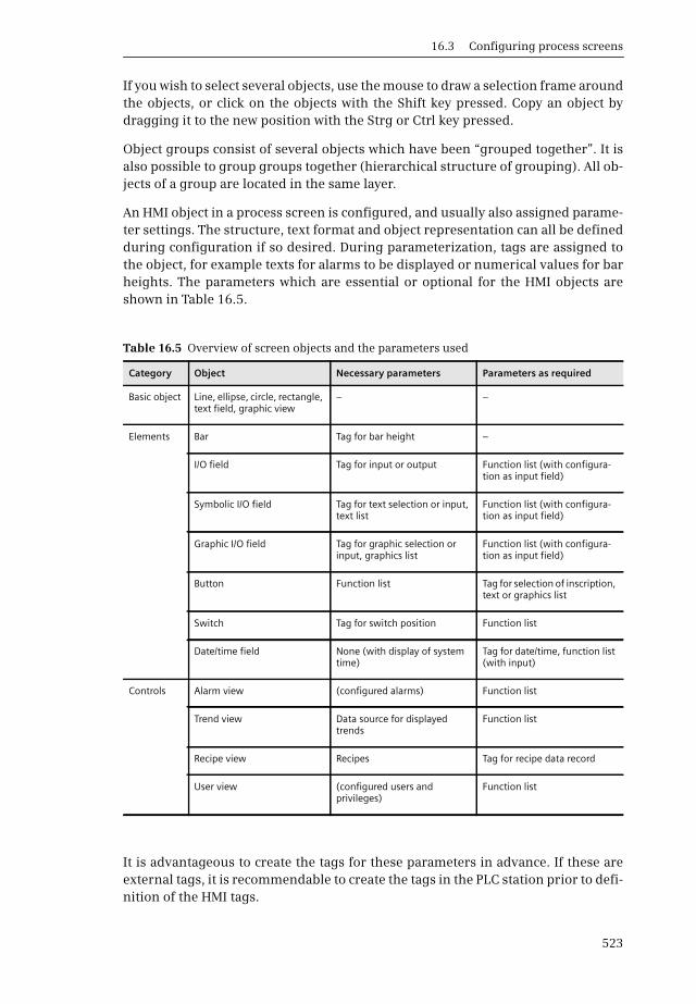
16.3 Configuring process screens
523
If you wish to select several objects, use the mouse to draw a selection frame aroundthe objects, or click on the objects with the Shift key pressed. Copy an object bydragging it to the new position with the Strg or Ctrl key pressed.
Object groups consist of several objects which have been “grouped together”. It isalso possible to group groups together (hierarchical structure of grouping). All ob-jects of a group are located in the same layer.
An HMI object in a process screen is configured, and usually also assigned parame-ter settings. The structure, text format and object representation can all be definedduring configuration if so desired. During parameterization, tags are assigned tothe object, for example texts for alarms to be displayed or numerical values for barheights. The parameters which are essential or optional for the HMI objects areshown in Table 16.5.
It is advantageous to create the tags for these parameters in advance. If these areexternal tags, it is recommendable to create the tags in the PLC station prior to defi-nition of the HMI tags.
Table 16.5 Overview of screen objects and the parameters used
Category Object Necessary parameters Parameters as required
Basic object Line, ellipse, circle, rectangle, text field, graphic view
– –
Elements Bar Tag for bar height –
I/O field Tag for input or output Function list (with configura-tion as input field)
Symbolic I/O field Tag for text selection or input, text list
Function list (with configura-tion as input field)
Graphic I/O field Tag for graphic selection or input, graphics list
Function list (with configura-tion as input field)
Button Function list Tag for selection of inscription, text or graphics list
Switch Tag for switch position Function list
Date/time field None (with display of system time)
Tag for date/time, function list (with input)
Controls Alarm view (configured alarms) Function list
Trend view Data source for displayed trends
Function list
Recipe view Recipes Tag for recipe data record
User view (configured users and privileges)
Function list

16 Visualization
524
16.3.9 Changing screen objects during runtime
The dynamic updating of screen objects is used to display changes or process se-quences in process screens. For example, the level in a tank can be displayed graph-ically depending on a process value. Predefined animations are available for thedynamic updating of the following object properties:
b Structure: the object changes its appearance, e.g. its color
b Position: the object moves in the screen
b Visibility: the object is displayed or hidden
b Operability: operator control of an object is enabled or locked
You can only configure one animation of the same type (movement, structure,visibility) for each object.
To configure an animation, select the object in the process screen and click in theinspector window in the Properties tab on the Animations tab. Select a new anima-tion by double-clicking on Add new animation in the tabbed browsing or selectingit from the overview. When adding, specify the tag whose value is to dynamize theobject property. The new animation is displayed in the Animations tab in the inspec-tor window.
When multiple objects have been selected, set the animations of the reference ob-ject in the inspector window. The settings apply to all objects which support theseanimations.
If you configure an animation for an object group, this animation applies to all in-dividual objects which support this animation.
16.3.10 Basic objects for screen configuration
The Basic objects category contains the following geometric objects: line, ellipse,circle and rectangle. The size, color, border type and filling pattern can be set de-pending on the object.
The group also contains a text field in which you can change, for example, the textstyle or the text, background and frame color, as well as a graphic view with a select-able graphic (Fig. 16.8).
Fig. 16.8 Basic objects in the Tools task card
Line Ellipse Circle Rectangle Text field Graphics view
Basic objects for process screen configuration
A
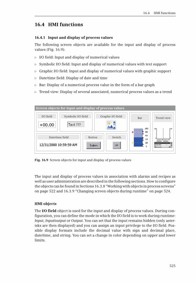
16.4 HMI functions
525
16.4 HMI functions
16.4.1 Input and display of process values
The following screen objects are available for the input and display of processvalues (Fig. 16.9):
b I/O field: Input and display of numerical values
b Symbolic I/O field: Input and display of numerical values with text support
b Graphic I/O field: Input and display of numerical values with graphic support
b Date/time field: Display of date and time
b Bar: Display of a numerical process value in the form of a bar graph
b Trend view: Display of several associated, numerical process values as a trend
The input and display of process values in association with alarms and recipes aswell as user administration are described in the following sections. How to configurethe objects can be found in Sections 16.3.8 “Working with objects in process screens”on page 522 and 16.3.9 “Changing screen objects during runtime” on page 524.
HMI objects
The I/O field object is used for the input and display of process values. During con-figuration, you can define the mode in which the I/O field is to work during runtime:Input, Input/output or Output. You can set that the input remains hidden (only aster-isks are then displayed) and you can assign an input privilege to the I/O field. Pos-sible display formats include the decimal value with sign and decimal place,date/time, and string. You can set a change in color depending on upper and lowerlimits.
Fig. 16.9 Screen objects for input and display of process values
I/O field Symbolic I/O field
SwitchButtonDate/time field
Bar
Screen objects for input and display of process values
Graphic I/O field Trend view

16 Visualization
526
The Symbolic I/O field object is used for the input or output of a process value withdisplay of a text. If the I/O field is configured as an input field, a value is assigned tothe configured tag depending on the displayed text which is selected from a text listduring runtime. With an output field, the text stored in a text list is displayed, de-pending on the value of a selection tag. Working with text lists is described in thenext section.
The Graphic I/O field object is used for the input or output of a process value withdisplay of a graphic. If the I/O field is configured as an input field, a value is assignedto the configured tag depending on the displayed graphic which is selected from agraphics list during runtime. With an output field, the graphic stored in a graphicslist is displayed depending on the value of a selection tag. Working with graphicslists is described in the next section.
The Date/time field object can be used to display and enter the date and/or time.The date/time tag can be the system time of the HMI station or an HMI tag.
The Button object is used to trigger a configurable action. A function list with sys-tem functions can be processed depending on the event (e.g. press, release). The in-scription can be text or a graphic, either fixed or selected from a text or graphics list.The processing of text, graphics and function lists is described in the next sections.
The Switch object enables the selection of two configurable states. The currentstate can be shown in the switch by a text or graphic. A function list with systemfunctions can be processed depending on events (e.g. switch ON, switch OFF).The processing of function lists is described in the section after next.
The Bar object displays a process value in graphic form. The display propertieswhich can be set include: the color response (change in color on violation of limits),the marking of limits, the division into bar segments, and the scale inscriptions anddivision.
The Trend view object displays tag values in the form of trends. You can set trenddisplay features with regard to position, geometry, style, color and font in the in-spector window. You can also specifically define whether a value table, a ruler or agrid is to be displayed in addition to the coordinate system.
Working with text and graphics lists
Text lists consist of individual texts which are assigned to the values of a tag. For ex-ample, a text list can be assigned as a selection list to a symbolic I/O field: if theI/O field is an input field, the tag assumes a specific value when a text is selected;if the I/O field is an output field, the corresponding text is displayed if the tag has aspecific value.
Graphics lists consist of individual graphics which are assigned to the values of atag. A graphic can be present in a graphics library or be an existing file in the stan-dard file format. Graphics lists are handled like text lists.

16.4 HMI functions
527
A multilingual configuration is possible for a text or graphics list, which is dis-played in the current operating during operation (runtime). This is meaningfule.g. for the graphic text of a graphics list.
To create a text or graphics list, double-click in the project tree under theHMI project on Text and graphics lists. Create the text lists in the Text lists tab, andthe graphics lists in the Graphics lists tab.
Double-click on <Add> in the table, and assign a meaningful name to the text orgraphics list. Select the list type under Selection which defines how the tag linked tothe list is to be interpreted:
b As Value/Range, then the text or graphic is displayed if the tag value is within the range or ranges
b As Bit (0, 1); a different text or graphic is then displayed for the signal states “0” and “1”
b As Bit number (0 to 31); texts or graphics are then assigned to the individual bits.
Then define the list contents. Select the list and enter the values of the tags and thetext or graphics in the Entries in text/graphics list table: Double-click on <Add> toopen a drop-down dialog box which depends on the range selection for thetext/graphics list:
b If Value/Range is selected, you can select Single value and enter the value or you select Range and specify the range; you can repeat this in the next lines with additional ranges or values
b If Bit is selected you can enter the texts/graphics for the signal states “0” and “1”
b If Bit number is selected you can enter the texts/graphics for the bit numbers 0 to 31
By activating Standard in the entries of the selection Value/Range and Bit num-ber, you define the text or graphic to be output if the tag assumes an undefinedvalue.
In the runtime settings under Screens you can define the response when severalbits are set as the bit number: if the Bit selection for text and graphics lists check boxis activated, the text or graphic that has been configured for a set bit with the leastsignificance is shown. If the check box is not activated, the text or graphic that hasbeen configured for a single set bit only is shown. If several bits are set, the text orgraphic set as standard is then shown.
16 Visualization
528
Working with function lists
System functions are predefined functions which cannot be changed, for examplefor calculating the value of a tag, for setting a bit in the PLC station, or for changingthe user.
An HMI object may have configurable events, e.g. a button has the Click event.A function list containing the system functions can be assigned to an event, whichare then executed when the event occurs.
To configure a function list, select the object in the process screen and open theEvents group in the Properties tab of the inspector window. Select an event, click inthe function list on <Add function> and select the desired system function from thedrop-down list.
It may be necessary to supply the system function with parameters. You can assignmore than one system function to an event.
16.4.2 Working with alarms
The alarm system distinguishes between system-defined alarms which do notrequire configuration and user-defined alarms which can be configured as analogalarms (display of limit violations) or discrete alarms (display of states or statuschanges).
System alarms indicate the status of the HMI station and of the communication be-tween the HMI and PLC station. The type and number depend on the HMI station.You can set the display duration of system alarms in the project tree under Runtimesettings and Alarms.
User-defined alarms visualize the process sequence and process states in themachine or plant. An alarm consists of an alarm number, the time of the event(date, time), the alarm text, the alarm status (incoming, outgoing), the alarm class,and possibly the alarm group (Fig. 16.10).
Alarms are assigned to certain Alarm classes: System (contains system-definedalarms for display of HMI station statuses), Errors (designed to display user-definedalarms for critical or dangerous statuses with an acknowledgment obligation) andWarnings (designed to display user-defined alarms for regular statuses without ac-knowledgment). User-defined alarm classes are configured with the desired repre-sentation and acknowledgment concept.
Alarms in an Alarm group are acknowledged together. Triggered alarm events aresaved in an alarm buffer. The Alarm view shows selected alarm events from thealarm buffer in a process screen. If a new alarm is present, the Alarm window showsall pending alarms or alarms awaiting acknowledgment of a particular alarm class.With an incoming alarm, the Alarm indicator shows the defined alarm class, andwhether unacknowledged alarms or alarms which have already been acknowledgedbut are still pending are still present.

16.4 HMI functions
529
Fig. 16.10 Components of the alarm system
Class GroupNumber Time stamp Status Alarm text
Alarm
1 Alarm2 Alarm3 Alarm
1 Alarm2 Alarm3 Alarm
Alarm text with output fields
Alarm text with output fields
Alarm view Alarm window Alarm indicator
Discrete alarm
Analog alarm
Variable text Variable number
Alarm system
Alarm without acknowledgment: if the alarm event arrives, the alarm is displayed until it goes again.
Alarm with acknowledgment: if the alarm event arrives, the alarm is displayed until it goes again and is acknowledged.
The alarm view is configured as an object in a process screen.
The alarm window is configured as a global window which opens and closes event-controlled irrespective of the current process screen.
The alarm indicator indicates the presence of unacknowledged or pending alarms independent of the current process screen.
An alarm can be acknowledged:
> Using the acknowledgment key in the alarm view or alarm window
> Using a button or a function key with the AlarmViewAcknowledgeAlarm system function
> Using a function key with the AcknowledgeAlarm system function.
Discrete alarms can be acknowledged by the PLC. Acknowledgment of a discrete alarm can be sent to the PLC.
A discrete alarm indicates a status change in the process. The change in status (the alarm event) is recorded by a trigger tag. The trigger tag is an external HMI tag of data type USHORT or SHORT. A trigger bit may only be used for one alarm.
An analog alarm indicates a limit violation in the process. The limit violation (the alarm event) is derived from a trigger tag. The alarm event is present if the trigger tag is above or below a configured limit which can be a constant or a tag.
The alarm number identifies the alarm.
The time stamp shows the date and time at which the alarm was triggered.
The alarm status has the events "incoming", "outgoing" and "Acknowledge".
The alarm text describes the cause of the alarm. It can include output fields for current values recorded at the time the status changed. These can be variable texts from a text list or variable process values.
The alarm class defines the acknowledgment concept and the representation of an alarm.
The alarm group combines alarms with a common acknowledgment.
The components of an alarm which are to be displayed can be configured.
? ?! !
Window title
!

16 Visualization
530
Alarm statuses
Each alarm has an alarm status (Table 16.6):
b Incoming (I) the condition for triggering an alarm applies
b Outgoing (O): the condition for triggering an alarm no longer applies
b Acknowledge (A): the user has acknowledged the alarm.
The display text of the message statuses can be freely selected.
Acknowledging alarms
Alarms without an acknowledgment obligation indicate process states which areneither critical nor dangerous. Alarms without an acknowledgment obligationcome and go without an acknowledgment.
Alarms with an acknowledgment obligation are used to ensure that the user hasregistered the occurrence of an alarm. By means of the acknowledgment, the userconfirms that the status which triggered the alarm has been processed. The alarmis displayed until it has been acknowledged. Alarms with an acknowledgment obli-gation indicate critical or hazardous states.
An alarm can be acknowledged on the HMI station by an authorized user or auto-matically by the system, e.g. by means of a tag value, a system function in a functionlist, or the program in the PLC station.
Alarms combined in an alarm group are acknowledged together. An alarm groupcan contain alarms from different classes. Examples of alarm groups are thosecaused by the same fault or those from a particular machine unit or subprocess.
Table 16.6 Alarm statuses
Alarms without acknowledgment obligation
Display text Status Description
I Incoming The condition of an alarm applies.
IO Outgoing The condition of an alarm no longer applies.
Alarms with acknowledgment obligation
Display text Status Description
I Incoming The condition of an alarm applies.
IO Outgoing, not acknowledged
The condition of an alarm no longer applies. The user has not acknowledged the alarm.
IOA Outgoing, then acknowledged
The condition of an alarm no longer applies. The user acknowl-edged the alarm after this point in time.
IA Incoming, acknowledged The condition of an alarm applies. The user has acknowledged the alarm.
IAO Outgoing, but acknowl-edged first
The condition of an alarm no longer applies. The user acknowl-edged the alarm when the condition still applied.

16.4 HMI functions
531
Configuring alarms
The steps for configuring alarms are as follows:
1) Create and edit alarm class (representation and acknowledgment concept)
2) If required: Create alarm groups (combination of alarms into groups that are acknowledged together)
3) Create tags (define tags and limits which are to trigger alarms)
4) Create alarms (configure discrete and analog alarms, and assign the tags, alarm class, alarm group etc. to be monitored)
5) Configure the alarm output (create HMI objects in process screens, and assign alarms)
6) If required: Configure loop-in-alarm (following the arrival of an alarm, the process screen in which the alarm event is present is selected)
To configure alarms, double-click on the HMI alarms editor in the project tree underthe HMI station.
Creating an alarm class
Select the Alarm classes tab in the HMI alarms window. The table already containsthe predefined alarm classes Errors, System, and Warnings. To enter a new alarmclass, double-clicking on <Add new> in the next line. You can specify its propertiesin the inspector window as required, in particular the acknowledgment concept andthe representation. You can configure enabling for the colored representation ofthe alarm classes in the project tree under Runtime settings > Alarms and General >Alarm class colors.
Creating an alarm group
Select the Alarm groups tab in the HMI alarms window. Double-click on <Add new>in the table to enter a new alarm group whose name you can change in the table cellor inspector window.
Configuring a discrete alarm
Select the Discrete alarms tab in the HMI alarms window (Fig. 16.11). To enter a newdiscrete alarm in the table, double-click on <Add new>. You can specify its proper-ties in the inspector window as required.
In the General section you can assign the alarm to an alarm class as well as to analarm group if required. Enter the event text which is to be displayed. You can inserttag output fields or text list output fields in the event text which display current val-ues or selected texts when the alarm is output. To do this, use the right mouse but-ton to select the position in the event text where the insertion is to take place, andthen select the output field in the shortcut menu. Then define the tag and the out-put format or the text list and the selection tag in the dialog.
In the Trigger section, select the tag whose change in status is to trigger the alarm.To do this, enter an HMI tag with the data type INT or UINT or a PLC tag with the
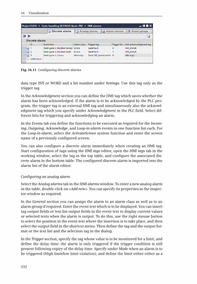
16 Visualization
532
data type INT or WORD and a bit number under Settings. Use this tag only as thetrigger tag.
In the Acknowledgment section you can define the HMI tag which saves whether thealarm has been acknowledged. If the alarm is to be acknowledged by the PLC pro-gram, the trigger tag is an external HMI tag and simultaneously also the acknowl-edgment tag which you specify under Acknowledgment in the PLC field. Select dif-ferent bits for triggering and acknowledging an alarm.
In the Events tab you define the functions to be executed as required for the Incom-ing, Outgoing, Acknowledge, and Loop-in-alarm events in one function list each. Forthe Loop-in-alarm, select the ActivateScreen system function and enter the screenname of a previously configured screen.
You can also configure a discrete alarm immediately when creating an HMI tag.Start configuration of tags using the HMI tags editor, open the HMI tags tab in theworking window, select the tag in the top table, and configure the associated dis-crete alarm in the bottom table. The configured discrete alarm is imported into thealarm list of the alarm editor.
Configuring an analog alarm
Select the Analog alarms tab in the HMI alarms window. To enter a new analog alarmin the table, double-click on <Add new>. You can specify its properties in the inspec-tor window as required.
In the General section you can assign the alarm to an alarm class as well as to analarm group if required. Enter the event text which is to be displayed. You can inserttag output fields or text list output fields in the event text to display current valuesor selected texts when the alarm is output. To do this, use the right mouse buttonto select the position in the event text where the insertion is to take place, and thenselect the output field in the shortcut menu. Then define the tag and the output for-mat or the text list and the selection tag in the dialog.
In the Trigger section, specify the tag whose value is to be monitored for a limit, anddefine the delay time: the alarm is only triggered if the trigger condition is stillpresent following expiry of the delay time. Specify under Mode when an alarm is tobe triggered (High limit/low limit violation), and define the limit either either as a
Fig. 16.11 Configuring discrete alarms

16.4 HMI functions
533
constant or as a tag. Synchronization indicates how the limits are synchronizedwith this alarm with regard to the limits configured for the tag (configured usingthe tag editor, see next section). By means of a deadband (hysteresis) you can pre-vent repeated generation of the alarm if the tag value oscillates around the limit(Fig. 16.12).
In the Events tab you define the functions to be executed as required for the Incom-ing, Outgoing, Acknowledge, and Loop-in-alarm events in one function list each. Forthe Loop-in-alarm, select the ActivateScreen system function and enter the screenname of a previously configured screen.
Configuring an analog alarm using the tag editor
You can also configure an analog alarm immediately when creating an HMI tag.Start configuration of tags using the Show all tags editor, open the HMI tags tab inthe working window, and select the tag in the top table. In the inspector window, en-ter high and low limits in the Properties tab under Range either as constants or tags.Configure the associated analog alarm in the bottom table in the working window.The configured analog alarm is imported into the alarm list of the alarm editor.
Configuring the alarm output
In order to display alarms, the Basic Panels feature the alarm view as an object in aprocess screen, the alarm window, and the alarm indicator.
Configuring an alarm view
An alarm view is configured in a process screen. You can configure the alarm states(pending or unacknowledged alarms) and the alarm classes in this alarm view.
Open the process screen and drag the Alarm view object from the Tools task cardunder the Control category into the screen. With the alarm view selected, you candesign its properties in the inspector window in accordance with your require-ments. You can make various settings in the Properties tab:
Fig. 16.12 Properties of an analog alarm (trigger conditions)

16 Visualization
534
b Under General you can select the alarm states to be displayed (pending and/orunacknowledged alarms) and activate the alarm classes to be displayed in thisalarm view.
b Under Display you can define the buttons to be shown in the alarm view (infotext,acknowledge, loop-in alarm) and whether a scroll bar is to be present.
b Under Layout you can set the number of lines for an alarm and how many alarmsare to be visible. You can also set the position and size of the alarm view here ifyou have not already done this with the mouse in the process screen. Use Layoutto define the (background) colors and, under Text format, the font size to beused.
b Under Columns you can define the visible columns and the sorting of alarms.
Configuring an alarm window
The alarm window shows the current alarms. It is opened independent of the cur-rent screen. The HMI station can still be used, even if alarms are present and dis-played. An alarm window is configured in the global screen and displayed like analarm view.
To configure the alarm window, double-click in the project tree under the HMIstation in the Screen management folder on Global screen. The global screenopens. It contains as standard the alarm window for unacknowledged alarms atscreen layer 1, for system alarms (active system events) at screen layer 1, and forpending (active) alarms at screen layer 3. You can also drag an additional alarmwindow from the Tools task card under the Controls category into the globalscreen.
In order to be able edit the alarm window better, position it in a separate screen lay-er, and hide the other layers (see Section 16.3.3 “Working with screen layers” onpage 519).
With the alarm view selected, you can design its properties in the inspector windowin accordance with your requirements. The settings are made as for the alarm view(see above). You can additionally select the properties of the window (Display auto-matically, Closable, Modal) and the inscription in the window title in the Propertiestab under Mode.
Configuring the alarm indicator
The alarm indicator indicates by means of a warning triangle that alarms are pend-ing or require acknowledgment. The alarm indicator flashes if at least one unac-knowledged alarm is present, and lights up continuously if at least one of the ac-knowledged alarms is not yet gone. The number of pending alarms is displayed.
To configure the alarm indicator, double-click in the project tree under the HMI sta-tion in the Screen management folder on Global screen. The global screen opens. Itcontains the warning triangle of the alarm indicator as standard. If the alarm indi-cator is not present, drag it from the Tools task card under the Controls category intothe open window. Only one alarm indicator is permissible.
16.4 HMI functions
535
With the alarm indicator selected, you set its properties in the inspector window:
b You select the alarm classes for the indicator in the Properties tab under General.The alarms from these alarm classes activate the indicator during runtime. Spec-ify whether pending alarms and/or alarms to be acknowledged are to be dis-played by the indicator.
b In the Events tab you can define whether the ShowAlarmWindow system functionis to be executed with Click or Click when flashing.
During runtime, the alarm indicator can only be accessed per touch screen.
Configuring the acknowledgment of alarms
Whether and how an alarm is acknowledged is defined in the alarm class to whichthe alarm is assigned (see Section “Creating an alarm class” on page 531). A pend-ing alarm can be acknowledged individually or in an alarm group. Acknowledg-ment can be performed in the following ways:
b Click the Acknowledge button in the alarm view or window.
b Configure a separate button or function key with the AlarmViewAcknowledgeAlarmsystem function for the Click or Press key event, and specify the alarm view whosealarm is to be acknowledged under Screen object.
b The acknowledgment of a discrete alarm by the PLC station, and the sending ofan acknowledgment bit to the PLC station, are described in Section “Configuringa discrete alarm” on page 531.
If acknowledgment of alarms is only to be allowed for a limited circle of users, con-figure a button or function key with a corresponding operator authorization(see Section 16.4.4 “Working with the user administration” on page 539).
16.4.3 Working with recipes
Recipes include associated data, for example data for a certain production batch.A recipe consists of recipe data records. These differ in terms of their values, but notin their structure. A recipe data record consists of recipe elements (Fig. 16.13).
You can enter the recipe data – if known – during the configuration phase. Recipesare saved in the HMI station and entered, modified or deleted in the recipe viewduring runtime.
The displayed recipe data record can be transferred to the PLC station. A recipe datarecord can also be transferred from the PLC station to the HMI station. The triggerfor this comes from a user or from the PLC station's program.
If there is a risk that recipe data could be mutually overwritten by the HMI andPLC stations, the transfer can be synchronized by means of the Data record areapointer.

16 Visualization
536
General procedure for configuring recipes
The structure of the recipe should be defined prior to the configuration of recipemanagement: What recipe elements are required per data record? How many datarecords does the recipe have? In which PLC tags are the values of the current datarecord to be saved?
Then create the PLC tags or the external HMI tags. Create a new recipe, define therecipe elements, and enter the data records with the values for each recipe element.
Configure a process screen with the recipe view. If the transfer of the current recipedata record to the PLC station is to be synchronized, create a Data record areapointer.
Creating a recipe
To configure a new recipe, first create the PLC tags for a recipe data record. If youdirectly select the PLC tags during the configuration phase when assigning thePLC tags to the recipe data record elements, external HMI tags are created automat-ically. You can also create the external HMI tags in advance and then select themduring configuration. Then create the new recipe, assign recipe elements to it, andenter the values for the elements in the data records.
Fig. 16.13 Recipe components
Data record 1
Recipe 1
External HMI tags (= recipe elements)
Data area in the PLC station
1 Recipe name 12 Recipe name 23 Recipe name 3
Recipe view
Recipe 2
Recipe n
Data record 2
Data record n
Displayed data record
(data record)
Element 1
Element 1
Element 1
Element 1
Element 1
Element 2
Element 2
Element 2
Element 2
Element 2
Element n
Element n
Element n
Element n
Element n
Recipes
…
……
…
…
…
A recipe is a combination of any type of data. Each recipe can have its own data structure.
A recipe consists of data records. Each data record of a recipe contains the same elements. The data records differ by the value (the contents) of their elements.
The recipe view on the HMI device is used to display, access and edit the recipes. The recipe list, data record list and element list can be displayed.
You can create, change, copy or delete a recipe data record. A recipe data record can be read from the PLC station or transferred to it.
The data record area pointer is used as necessary to coordinate the transfer of a recipe data record between the HMI and PLC stations.
16.4 HMI functions
537
Double-click on the Recipes editor in the project tree under the HMI station. The dis-played recipe list has two parts: The top part Recipes lists the recipes. In the bottompart you can enter the elements of a recipe data record in the Elements tab and inthe Data records tab you can define the number of data records in the recipe.
Create a new recipe in the Recipes table. In the properties of the recipe in theinspector window, you define under Synchronization whether data exchange is tobe synchronized and via which HMI connection this is to be carried out. If the Coor-dinated data transfer checkbox is activated, the Data record area pointer must beconfigured.
Enter the recipe elements in the Elements table. A double-click on <Add> creates aline with a new element. In the Tag column, assign either an external HMI tag or adirect PLC tag to the recipe element. During runtime, these tags save the value ofthe recipe element in the current recipe data record. The value in the Default valuecolumn is used as the default entry when creating a data record. A recipe elementcan be assigned a text list whose text, depending on the value of the recipe element,is displayed during runtime in an output field. Enter as many elements as presentin a recipe data record.
In the Data records table, define the values of the recipe elements for each individ-ual data record. A double-click on <Add> creates a line with a new data record witha column for each recipe element. Enter the values for the recipe elements here.
Configuring a recipe view
The recipe view is an off-the-shelf display and control element used to manage rec-ipe data records.
To configure the recipe view in a process screen, use the mouse to drag the recipeview from the Tools task card under the Controls category into the open screen.
If you only wish to display a particular recipe in the view, enter the recipe underGeneral in the properties of the recipe view in the inspector window. You can specifya tag in the Recipe data record section in which – depending on the tag's dataformat – the number or name of the currently displayed recipe data record is to besaved. If you deactivate the Editing mode check box, you can suppress the editing ofrecipe data, and the data is only displayed.
You define the display of the recipe data under Simple view. Under Toolbar you candefine which buttons are to be available in the recipe view during runtime.
Operating the recipe view during runtime
You can display the list of all existing recipes, the data record list of a recipe, andthe element list for a data record in the recipe view. The view always begins with therecipe list. Depending on the configuration, you can create a new recipe data re-cord, modify, copy or delete an existing record, transfer a record to the PLC station,or read a record from the PLC station.

16 Visualization
538
The values of a data record modified in the recipe view must be transferred to thePLC station to enable them to be processed there. To carry out the transfer, open thedesired recipe and the elements list of the data record whose values you wish totransfer. Select the Down command in the shortcut menu.
In order to read the values of a recipe data record from the PLC station, open therecipe and the elements list of the data record whose values are to be imported fromthe PLC station. Select the Up command in the shortcut menu. The new values aredisplayed.
You can also assign the commands of the recipe view to another screen object. Forexample, you can assign the RecipeViewSetDataRecordToPLC system function to abutton or function key.
Controlling transfer from PLC station's program
Using the Job mailbox area pointer you can read a recipe data record from the PLCstation (job number 69) or write one into the PLC station (job number 70). Work-ing with area pointers is described in Section 16.2.3 “Creating an area pointer” onpage 515. The first parameter of the area pointer contains the recipe number, thesecond parameter the data record number. During transfer from the PLC station tothe HMI station (job number 69) you can specify in the third parameter whetherthe existing data record is to be overwritten (with 1) or not (with 0).
The recipe view is not updated automatically. For example, if recipe data is trans-ferred from the PLC station while the recipe is being displayed, the new values areonly displayed when the associated data record is selected again.
Synchronized transfer to the PLC station
There are two possibilities for the transfer: transfer without synchronization andtransfer with synchronization via the Data record area pointer. You can use transferwithout synchronization if the transfer of a data record is to be exclusively trig-gered by an operator input on the HMI station. Synchronization is necessary if thetransfer is triggered from both the HMI station and PLC station. This preventsuncontrolled mutual overwriting of data.
If the initiative for transfer comes from the HMI station, it enters a value of 2 intothe status word, changes the recipe and data record numbers, reads or writes thedata record values, and sets the status word to a value of 4. The PLC station mustset the status word to 0 in order to enable the next transfer.
If the initiative comes from the PLC station, this must trigger the HMI station totransfer by means of control job no. 69 or no. 70 (as described above). The furthersequence is as with the initiative from the HMI station.
A bit in the status word may only be set by the HMI station. The PLC station may on-ly reset the status word back to 0.

16.4 HMI functions
539
16.4.4 Working with the user administration
You configure user groups, users, and authorizations with the user administration.Authorizations restrict security-related operations to specific user groups. To dothis, set up access protection for the operating element; then only a user assignedto a user group with the relevant access rights can perform the operation using thisobject (Fig. 16.15).
Examples of user groups with different privileges include: Administrators or Serviceengineers who have unlimited access, Technicians who are permitted to make set-tings in the process or on the machine, and Operators who are responsible for theproduction process.
Configuration procedure
1) User groups are defined during the configuration phase. If users are alreadyknown at this point in time, they can be included in a user group. Users can alsobe assigned to the user group during runtime by means of the User view.
2) Define privileges, and assign the corresponding privileges to each user group.
3) During configuration of the operator-accessible object, set the privilege withwhich this object can be accessed in the properties under Security. This meansthat a user can only operate this object during runtime if he or she is included inthe corresponding user group.
Configuring users and user groups
To configure the user administration, double-click in the project tree under the HMIstation on User administration and select the User groups tab in the working win-dow. The Administrator group and Users user groups are always present in the top
Fig. 16.14 Structure of the Data record area pointer
Data record area pointer Value of status word
Current recipe number (1 … 999)
Reserved Transfer busy
Status (0, 2, 4, 12) Successfully completed
Reserved Completed with errors
Current data record number (1 … 65 535) Transfer permissible
Word 1 Decimal Binary Meaning
Word 2 0 0000 0000
Word 3 2 0000 0010
Word 4 4 0000 0100
Word 5 12 0000 1100
Data record area pointer
The data record area pointer is used to synchronize the transfer of a recipe data record. It can be created in the PLC station as a tag of data type ARRAY [1..5] of UINT.
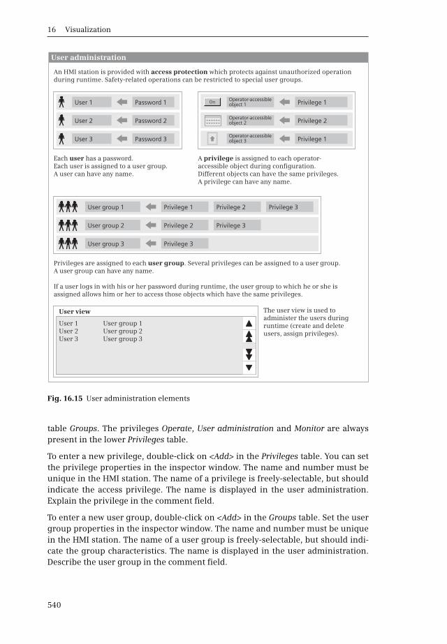
16 Visualization
540
table Groups. The privileges Operate, User administration and Monitor are alwayspresent in the lower Privileges table.
To enter a new privilege, double-click on <Add> in the Privileges table. You can setthe privilege properties in the inspector window. The name and number must beunique in the HMI station. The name of a privilege is freely-selectable, but shouldindicate the access privilege. The name is displayed in the user administration.Explain the privilege in the comment field.
To enter a new user group, double-click on <Add> in the Groups table. Set the usergroup properties in the inspector window. The name and number must be uniquein the HMI station. The name of a user group is freely-selectable, but should indi-cate the group characteristics. The name is displayed in the user administration.Describe the user group in the comment field.
Fig. 16.15 User administration elements
User 1 User group 1User 2User 3
User group 2User group 3
User view
User 1 Password 1
User 2 Password 2
User 3 Password 3
User group 1
Operator-accessible object 1
Operator-accessible object 2
Operator-accessible object 3
Privilege 1
Privilege 1 Privilege 2 Privilege 3
Privilege 2
Privilege 2 Privilege 3
Privilege 1
Privilege 3
User group 2
User group 3
User administration
An HMI station is provided with access protection which protects against unauthorized operation during runtime. Safety-related operations can be restricted to special user groups.
The user view is used to administer the users during runtime (create and delete users, assign privileges).
Each user has a password. Each user is assigned to a user group. A user can have any name.
A privilege is assigned to each operator-accessible object during configuration. Different objects can have the same privileges. A privilege can have any name.
Privileges are assigned to each user group. Several privileges can be assigned to a user group. A user group can have any name.
If a user logs in with his or her password during runtime, the user group to which he or she is assigned allows him or her to access those objects which have the same privileges.
On

16.4 HMI functions
541
To assign privileges to a user group, select the user group and activate the corre-sponding privileges in the Active column in the Privileges table.
In the Users tab, configure the users in the top table Users. One user Administratoris already present. Double-click on <Add> and enter the properties of the next userin the inspector window. The name and number must be unique in the HMI station.Assign a password and confirm it. A user can change his or her own passwordduring runtime.
To assign the user to a user group, select the user and then the user group in theMember of column in the Groups table. You can assign a user to exactly one usergroup. In the inspector window, you can set in the user properties under Automaticlogoff the number of minutes after which automatic logging off is to take place.
Configuring access protection for control elements
The privileges created in the user administration must be assigned to the controlelements protected against unauthorized access. Objects with access protection arethe date/time field, the I/O field, the graphic and symbolic I/O fields, the switch, thebutton, and the recipe view.
In order to configure access protection for a control element, open the processscreen and select the control element. In the inspector window, select the privilegeunder Properties and Security, and define whether operator access is permissible.
Configuring the user view
The user view is used to configure and administer users and privileges during run-time. The user view is configured in a process screen. Open the screen and use themouse to drag the user view from the Tools task card under Controls into the screen.Set the user view properties in the inspector window.
Runtime settings for user administration
Use the Runtime settings editor under an HMI station in the project tree to configurethe security settings of the user administration during runtime. Start by double-clicking on the editor, and select the User administration section in the runtime set-tings.
Under General you set the number of permissible invalid login attempts by a userbefore the user is assigned to the Unauthorized group. If the Logon only with pass-word checkbox is activated, users are not required to enter a user name when log-ging in.
Under Hierarchy level you can activate the group-specific privileges for the user ad-ministration. This means that an administrator can only administer those usersduring runtime whose group number is smaller than or equal to his or her ownnumber, and only assign a user to a user group whose number is smaller than orequal to his or her own group number.

16 Visualization
542
Under Password, you can activate the password aging. You can set the number ofdays for which a password is valid, and the preliminary warning time before achange in password becomes necessary. Password generation is understood to bethe number of past passwords before a certain password can be repeated. Withpassword aging activated, the Password aging column can be edited for the usergroups (User administration editor in the Users tab and Groups table).
Under Password complexity you can set the minimum password length and alsospecify whether a password must contain digits and/or special characters.
16.5 Completing HMI configuration
16.5.1 Compiling the HMI configuration (Consistency test)
The entered configuration data must be compiled so that execution in the HMI sta-tion is possible. During configuration the data is compiled continuously in thebackground. Further compilation takes place automatically when downloading tothe HMI station.
You can also compile the configuration data in between times in order to check itsconsistency. The faulty positions are listed in the inspector window and can be direct-ly selected by double-clicking on the error message in order to eliminate the error.
To compile the entire configuration data for an HMI station, select the stationand then the Compile > Software (rebuild all) command in the shortcut menu. TheCompile > Software command is used to compile only the configuration data whichhas been changed since the last compilation. If the PLC tags were changed duringcompilation of the HMI device, or if new ones have been added, it is advisable to alsocompile the corresponding data blocks in the PLC station prior to compilation ofthe HMI configuration.
16.5.2 Simulation of HMI configuration
You can use the simulator on the programming device to test the response of theHMI configuration. The simulation can be carried out together with the PLC stationor with the tag values of a simulation table, in the latter case without a PLC station.
To carry out the simulation, select the HMI station in the project tree and then theOnline > Simulation > … command from the main menu.
The command Online > Simulation > Start starts the simulation with the networkedPLC station. The simulator program establishes a connection to the active PLC sta-tion and imports its tag values for the simulation. The configured process screensare displayed in the simulator window. Use the mouse for operations instead of thetouch screen and function keys.
The command Online > Simulation > With tag simulator starts the simulation withsimulation table. Two windows are opened: simulation of the HMI configuration

16.5 Completing HMI configuration
543
(display of the process screens) and the simulation table. Use the <Alt + Tab> keycombination to switch between the two windows.
Enter all tags in the simulation table with which you wish to simulate the HMI con-figuration. The Format column defines the display format, the Set value column thestart value. In the Simulation column, select the type of simulation, e.g. Increment,from the drop-down list. Enter the value by which the tag value is to change in theCycle column. Define the rate of change in the Write cycle column: the value enteredcorresponds to the interval in seconds with which the tag value is to be changed.In the MinValue and MaxValue columns you can define the range of values for tags.In order to carry out simulation with a tag, activate the Start check box.
Depending on the data type of the tag, the simulator provides six different modes(Fig. 16.16):
b Sinus: changes the value in the form of a sinusoidal curve
b Random: provides randomly generated values
b Increment: increases the tag value commencing with the start value up to themaximum value, and commences again with the minimum value
b Decrement: decreases the tag value commencing with the start value down to theminimum value, and commences again with the maximum value
b Shift bit: shifts a set bit continuously by one position
b <Display>: shows the current tag value in static form
You can save the settings of the simulation table using the menu command File >Save. Several simulation tables with different contents can be saved. Use File > Opento open a saved simulation table again.
16.5.3 Downloading configuration to the HMI station
You have created a project with a PLC and an HMI station. The PLC and HMI stationare networked and prepared for data exchange with at least one HMI connection.The user program in the PLC station is complete, compiled, and downloaded to thePLC station (Chapter 13.2 “Transferring project data” on page 425). Configuration
Fig. 16.16 Example of a simulation table
16 Visualization
544
of the HMI station has been completed, the configuration data has been compiled,and – as far as possible – successfully simulated.
Preparation for loading the configuration data
The standard settings for loading are defined in the properties of the HMI station.Select the HMI station in the project tree and then the Properties command in theshortcut menu. The settings which you already made when networking the PLC sta-tion are present in the properties window in the Ethernet addresses section.
You can assign an IP address online to an HMI station if you start the Online & diag-nostics editor in the project tree under the HMI station. You set the IP address andsubnet mask in the working window under Functions and Assign IP address. Use theAssign IP address button to transfer the settings to the HMI station.
Checking the connection data on the HMI station
You can check the connection settings on the HMI station in the Control Panel. Ifyou start the HMI station (connect the power supply) the loader window is displayedduring booting. If configuration data is already loaded and the root screen is dis-played, terminate the runtime (the current program on the HMI device) using a cor-respondingly configured function key or using the system screen Different jobs inorder to display the loader window.
Click in the loader window on the Control Panel button. Briefly click twice to reachthe next dialogs in the Control Panel: Profinet and Transfer contain the network set-tings, e.g. the IP address. To change an entry, click on the associated field and enterthe new value using the on-screen keyboard which appears. Exit the Control Panelby clicking on the exit cross at the top right in the title bar.
Downloading configuration data
To download, select the HMI station in the project tree and choose the commandDownload to device > Software (all) from the shortcut menu. In the Extended down-load to device dialog, you can specify the IP address of the HMI station to be loadedto (Fig. 16.17).
The configuration data is compiled on downloading. Displayed warnings do notprevent downloading; the function may be restricted at runtime. If there are errors,the configuration data is not loaded. Clear any faults before trying to downloadagain.
After successful compilation, the downloading preview is displayed. You see theindividual loading steps and can change specific settings as required. If the com-pilation is completed without errors – and you have activated the settings to over-write the user administration and recipe data, if required – click on the Load but-ton. The messages that appear during loading are displayed in the inspector win-dow in the Info tab.
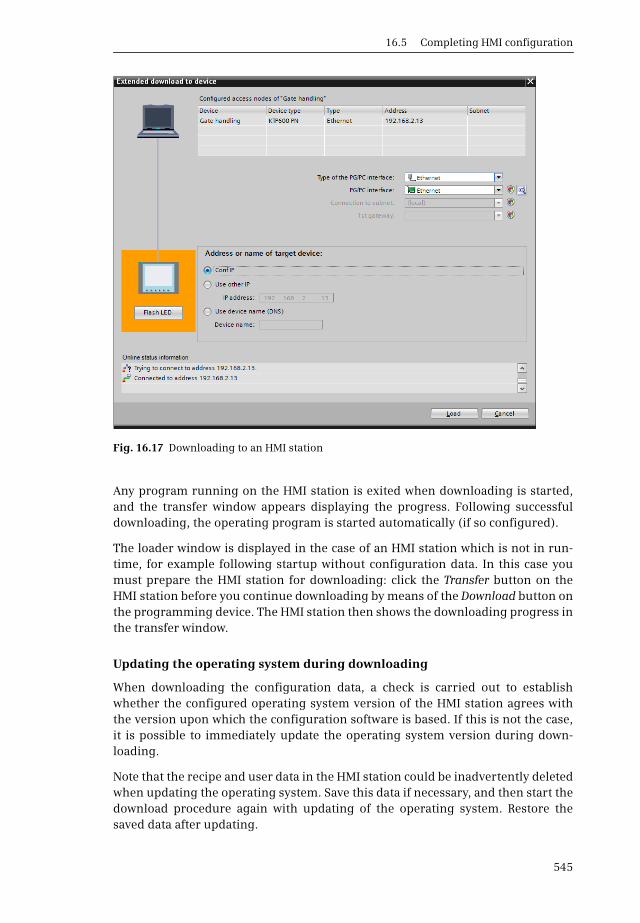
16.5 Completing HMI configuration
545
Any program running on the HMI station is exited when downloading is started,and the transfer window appears displaying the progress. Following successfuldownloading, the operating program is started automatically (if so configured).
The loader window is displayed in the case of an HMI station which is not in run-time, for example following startup without configuration data. In this case youmust prepare the HMI station for downloading: click the Transfer button on theHMI station before you continue downloading by means of the Download button onthe programming device. The HMI station then shows the downloading progress inthe transfer window.
Updating the operating system during downloading
When downloading the configuration data, a check is carried out to establishwhether the configured operating system version of the HMI station agrees withthe version upon which the configuration software is based. If this is not the case,it is possible to immediately update the operating system version during down-loading.
Note that the recipe and user data in the HMI station could be inadvertently deletedwhen updating the operating system. Save this data if necessary, and then start thedownload procedure again with updating of the operating system. Restore thesaved data after updating.
Fig. 16.17 Downloading to an HMI station

16 Visualization
546
Saving and restoring are described in the next Section 16.5.4 “Maintenance of theHMI station”. Updating of the operating system can also be carried out independentof downloading.
Starting the HMI station
Following successful downloading of the configuration data, the runtime starts fol-lowing a certain delay, if so configured. You can configure the delay time on theHMI station: click in the loader window on the Control Panel button, double-click inthe Control Panel on OP, and set the delay time in seconds in the OP propertieswindow in the Display tab (click on the input field).
The runtime also starts if you click on the Start button in the loader window.
16.5.4 Maintenance of the HMI station
Maintenance of the HMI station comprises the following functions:
b Save configuration data of HMI station
b Restore configuration data of HMI station
b Authorization/licensing (does not apply to Basic Panels)
b Update operating system
b Options (does not apply to Basic Panels)
To start a maintenance function, select an HMI station and use the main menu com-mand Online > Device maintenance > … in the project tree.
Data backup
Using a connected programming device you can save the following HMI stationdata: Complete backup (all data including operating system), recipes, and useradministration (Fig. 16.18).
Fig. 16.18 Saving configuration data and operating system

16.5 Completing HMI configuration
547
Start STEP 7 Basic, open the project with the HMI station whose data is to be saved,and select the HMI station in the project tree. Check that the settings for down-loading are correct in the properties of the HMI station (in the Properties shortcutmenu, and then select the Download section).
In the main menu, select Online > HMI device maintenance > Backup. Perform thesave operation for the desired data type. To restore the data, select Online > HMIdevice maintenance >Restore in the main menu.
Updating the operating system of the HMI station
When updating the operating system, all data on the HMI station is deleted.You must save the data for recipes or user administration if you wish to use themagain following updating of the operating system.
Start the operating system update by selecting an HMI station in the project treeand choosing Online > HMI device maintenance >Update operating system from themain menu.
A connection to the HMI station is established using the Device status button. Therelevant device data is displayed: the boot loader and operating system versions aswell as the sizes of the flash and RAM memories.
If you wish to reset the HMI station to the default settings, e.g. because updating ofthe operating system was interrupted, activate the Reset to default settings checkbox in the ProSave window.
17 Appendix
548
17 Appendix
17.1 Integral and technological functions
17.1.1 High-speed counter (HSC)
Contrary to a counter function, a high-speed counter (HSC) counts pulses inde-pendent of the cycle time of the user program. A counting frequency up to200 kHz is possible. The counting range corresponds to the range of values of aDINT tag (–2 147 483 648 to +2 147 483 647).
A high-speed counter is an integral component of the CPU and must be activatedand configured prior to use. The number of available high-speed countersdepends on the CPU: three counters for the CPU 1211, four counter for the CPU1212, and six counters for the CPU 1214 and CPU 1215. The number of high-speedcounters with the CPU 1211 and CPU 1212 can be increased by using a signalboard with digital input channels.
A high-speed counter can be used as a single-phase or two-phase counter (A/Bquadrature). Please note that – depending on the operating mode – specific inputchannels are permanently assigned to a high-speed counter and that this may re-sult in limitations when using the counter. The assignment of the counter inputs af-fects the peripheral inputs (the input terminals). A change in the (logical) input ad-dresses has no influence on this assignment.
With correspondingly designed signal boards, the maximum counting frequencyof 100 kHz achievable with the onboard inputs of the CPU can be increased to200 kHz.
The data required for execution of a counter function is saved in a data block. Whencalling the counter function as a single instance, this is a separate data block percall, when calling as a local instance in a function block, the instance data block ofthe function block can be used for data saving (multi-instance).
Assignment of inputs to high-speed counters
Depending on the operating mode, specific inputs integrated on the CPU or on thesignal board are assigned to a high-speed counter (Table 17.1). If a counter uses theinputs, they cannot be used elsewhere. Unused inputs can be used like “normal”inputs for other purposes. Inputs used by a high-speed counter cannot be forced(assigned a fixed value).
As the table shows, the assignable inputs of HSC 1 and HSC 2 (I 0.1, I 0.3) as well asof HSC 3 and HSC 4 (I 0.5, I 0.7) overlap, meaning that not all counters can be usedin every mode. If both counters are to be used in each case, it is possible to change

17.1 Integral and technological functions
549
back to the inputs of the signal board or adapt the operating modes. For example,control of the counting direction and resetting can also be carried out with theCTRL_HSC statement as an alternative to the external inputs.
Fig. 17.1 shows which inputs and outputs are used by a high-speed counter depend-ing on the operating mode.
Table 17.1 Assignment of onboard inputs to counters (without signal board)
CPU input HSC No. For single-phase counter mode
For two-phase counter mode
For A/B quadrature mode
I 0.0 HSC 1 Clock input Clock input up Clock phase A
I 0.1 HSC 1HSC 2
DirectionReset
Clock input downReset
Clock phase BClock phase Z
I 0.2 HSC 2 Clock input Clock input up Clock phase A
I 0.3 HSC 1HSC 2
ResetDirection
ResetClock input down
Clock phase ZClock phase B
I 0.4 HSC 3 Clock input Clock input up Clock phase A
I 0.5 HSC 3HSC 4
DirectionReset
Clock input downReset
Clock phase BClock phase Z
I 0.6 HSC 4 Clock input Clock input up Clock phase A
I 0.7 HSC 3HSC 4
ResetDirection
ResetClock input down
Clock phase ZClock phase B
I 1.0 HSC 5 Clock input Clock input up Clock phase A
I 1.1 HSC 5 Direction Clock input down Clock phase B
I 1.2 HSC 5 Reset Reset Clock phase Z
I 1.3 HSC 6 Clock input Clock input up Clock phase A
I 1.4 HSC 6 Direction Clock input down Clock phase B
I 1.5 HSC 6 Reset Reset Clock phase Z
Fig. 17.1 Inputs and outputs of a high-speed counter
Single-phase counter
Two-phase counter, A/B quadrature
Clock input
Reset
Direction
Reset
Clock input 1
Clock input 2
Actual count value = reference value
Change in counting direction
External reset
Actual count value
Inputs and outputs of a high-speed counter (HSC)
Pulse train
Pulse train 1 or phase A
In the peripheralinput area
Process interrupt event
Process interrupt event
Process interrupt event
Alternatively: externalcounting direction control
Pulse train 2 or phase B
Optional: external settingto the initial count value
Optional: external setting to the initial count value

17 Appendix
550
Operating modes of a high-speed counter
Fig. 17.2 shows the possible counting modes of a high-speed counter.
Single-phase counter: the counter is controlled by a single pulse train. The countingdirection is specified either internally with the CTRL_HSC statement or externallyvia an input. Each rising edge of a pulse increases or decreases the count value de-pending on the actual counting direction.
Two-phase counter: The counter is controlled by two independent pulse trains, onefor the up counting direction and one for the down counting direction. Each risingedge of a pulse increases or decreases the count value depending on the pulse train.Please note that with the first pulse of the other input in each case, there is a changein the counting direction and therefore – if activated – the associated process inter-rupt will be triggered.
A/B quadrature with single speed: The counter is controlled by two pulse trains offsetby 90° (“Phase A” and “Phase B”). If the pulse train of phase B has signal state “0”(“between” the pulses), counting is enabled: then each rising edge of the pulses ofphase A results in an increase in the count value, and each falling edge a decrease.
A/B counter with quadruple speed:The counter is controlled by two pulse trains off-set by 90° (“Phase A” and “Phase B”). Each edge of each pulse train is counted.
Fig. 17.2 Operating modes of a high-speed counter
Operating modes of a high-speed counter (HSC)
Single-phase counter
Two-phase counter
A/B quadrature (1x)
A/B quadrature (4x)
Clock input
Clock input up
Clock phase A
Clock phase A
Clock input down
Clock phase B
Clock phase B
Counts one pulse with counting direction up
Counts one pulse with counting direction down
Counts one pulse with the set counting direction
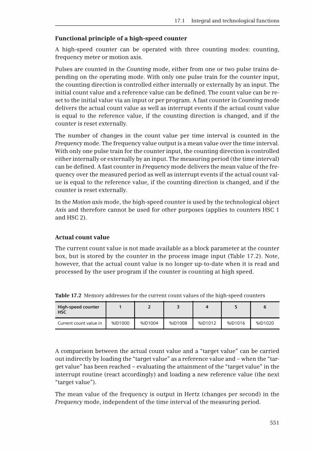
17.1 Integral and technological functions
551
Functional principle of a high-speed counter
A high-speed counter can be operated with three counting modes: counting,frequency meter or motion axis.
Pulses are counted in the Counting mode, either from one or two pulse trains de-pending on the operating mode. With only one pulse train for the counter input,the counting direction is controlled either internally or externally by an input. Theinitial count value and a reference value can be defined. The count value can be re-set to the initial value via an input or per program. A fast counter in Counting modedelivers the actual count value as well as interrupt events if the actual count valueis equal to the reference value, if the counting direction is changed, and if thecounter is reset externally.
The number of changes in the count value per time interval is counted in theFrequency mode. The frequency value output is a mean value over the time interval.With only one pulse train for the counter input, the counting direction is controlledeither internally or externally by an input. The measuring period (the time interval)can be defined. A fast counter in Frequency mode delivers the mean value of the fre-quency over the measured period as well as interrupt events if the actual count val-ue is equal to the reference value, if the counting direction is changed, and if thecounter is reset externally.
In the Motion axis mode, the high-speed counter is used by the technological objectAxis and therefore cannot be used for other purposes (applies to counters HSC 1and HSC 2).
Actual count value
The current count value is not made available as a block parameter at the counterbox, but is stored by the counter in the process image input (Table 17.2). Note,however, that the actual count value is no longer up-to-date when it is read andprocessed by the user program if the counter is counting at high speed.
A comparison between the actual count value and a “target value” can be carriedout indirectly by loading the “target value” as a reference value and – when the “tar-get value” has been reached – evaluating the attainment of the “target value” in theinterrupt routine (react accordingly) and loading a new reference value (the next“target value”).
The mean value of the frequency is output in Hertz (changes per second) in theFrequency mode, independent of the time interval of the measuring period.
Table 17.2 Memory addresses for the current count values of the high-speed counters
High-speed counter HSC
1 2 3 4 5 6
Current count value in %ID1000 %ID1004 %ID1008 %ID1012 %ID1016 %ID1020

17 Appendix
552
Configuring a high-speed counter
A high-speed counter must be activated using the hardware configuration editor.In order to configure a high-speed counter, start the Device configuration editor un-der the PLC station in the project tree. Select a high-speed counter in the propertiesof the CPU module in the inspector window, and activate it using the Enable thishigh-speed counter for use check box.
You set the counting mode (counting, frequency, or axis of motion) under Func-tion and under Operating phase you set the manner in which the count pulses areto be made available and counted (single-phase, two-phase, A/B counter 1X, A/Bcounter 4X). If a signal board is plugged in, you can select the input source (inte-grated CPU input, signal board input) for the HSC 1, HSC 2, HSC 5, and HSC 6counters. The inputs of a counter (counter input, direction input, reset input) areeither all on the CPU or all on the signal board. If you have selected Single-phasefor the operating phase, set under Counting direction is specified by whether thecounting direction is to be defined by the user program (internal direction con-trol) or by an input (external direction control). Define the initial counting direc-tion.
Under Reset to initial values you can define the initial count value and the initial ref-erence value and define whether resetting to these values is to be carried out by anexternal input and at which signal level. Resetting is active for as long as the set sig-nal level is present. You can change the initial count value and the reference valueduring runtime using the CTRL_HSC statement.
Under Event configuration you can set the event at which the counter is to generatea process interrupt, as well as the name of the interrupt event. The events are:Generate interrupt for counter value equals reference value event, Generate interruptfor external reset event and Generate interrupt for direction change event. Provide theevent with a name, and assign a process interrupt organization block to it.The HW interrupt drop-down list contains all previously created organizationblocks with the start event Hardware interrupt. You can create a new process inter-rupt OB using the Add object button.
Hardware inputs lists those inputs occupied by counters, together with the maxi-mum achievable counting frequency.
Under I/O addresses/HW identifier you can set the addresses of the peripheral inputsat which the counter is to output the actual count value. In the Process imagedrop-down list you can set whether the transfer is to be to the input process image(Cyclic PI). The hardware ID of the counter is also specified in this tab (HW ID); usethis for assigning the configured counter to the CTRL_HSC statement on theHSC parameter.
CTRL_HSC statement
The CTRL_HSC statement controls a high-speed counter. CTRL_HSC can be foundin the program elements catalog under Technology and Counters. To call the state-ment, drag CTRL_HSC with the mouse into the open block. Each CTRL_HSC call
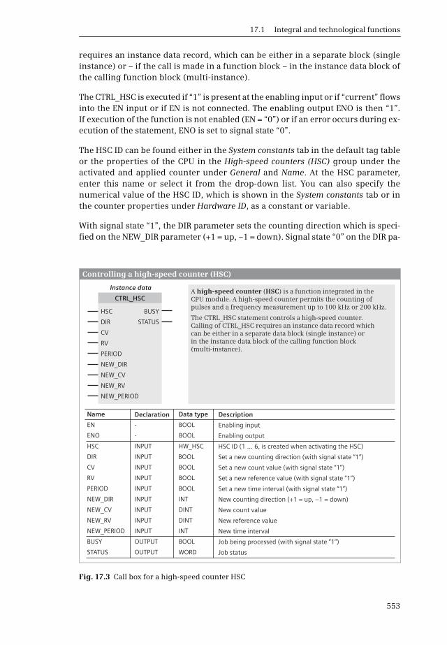
17.1 Integral and technological functions
553
requires an instance data record, which can be either in a separate block (singleinstance) or – if the call is made in a function block – in the instance data block ofthe calling function block (multi-instance).
The CTRL_HSC is executed if “1” is present at the enabling input or if “current” flowsinto the EN input or if EN is not connected. The enabling output ENO is then “1”.If execution of the function is not enabled (EN = “0”) or if an error occurs during ex-ecution of the statement, ENO is set to signal state “0”.
The HSC ID can be found either in the System constants tab in the default tag tableor the properties of the CPU in the High-speed counters (HSC) group under theactivated and applied counter under General and Name. At the HSC parameter,enter this name or select it from the drop-down list. You can also specify thenumerical value of the HSC ID, which is shown in the System constants tab or inthe counter properties under Hardware ID, as a constant or variable.
With signal state “1”, the DIR parameter sets the counting direction which is speci-fied on the NEW_DIR parameter (+1 = up, –1 = down). Signal state “0” on the DIR pa-
Fig. 17.3 Call box for a high-speed counter HSC
CTRL_HSC
PERIOD
HSC
NEW_DIR
DIR
NEW_CV
CV
NEW_RV
RV
NEW_PERIOD
BUSY
STATUS
Controlling a high-speed counter (HSC)
Instance data A high-speed counter (HSC) is a function integrated in the CPU module. A high-speed counter permits the counting of pulses and a frequency measurement up to 100 kHz or 200 kHz.
The CTRL_HSC statement controls a high-speed counter. Calling of CTRL_HSC requires an instance data record which can be either in a separate data block (single instance) or in the instance data block of the calling function block (multi-instance).
DeclarationName
EN
ENO
HSC
DIR
CV
RV
NEW_RV
PERIOD
NEW_PERIOD
NEW_DIR
BUSY
NEW_CV
STATUS
-
-
INPUT
INPUT
INPUT
INPUT
INPUT
INPUT
INPUT
INPUT
OUTPUT
INPUT
OUTPUT
BOOL
BOOL
HW_HSC
BOOL
BOOL
BOOL
DINT
BOOL
INT
INT
BOOL
DINT
WORD
Enabling input
Enabling output
HSC ID (1 ... 6, is created when activating the HSC)
Set a new counting direction (with signal state “1”)
Set a new count value (with signal state “1”)
Set a new reference value (with signal state “1”)
New reference value
Set a new time interval (with signal state “1”)
New time interval
New counting direction (+1 = up, –1 = down)
Job being processed (with signal state “1”)
New count value
Job status
DescriptionData type

17 Appendix
554
rameter has no effect. The parameter is only effective if the counter is configuredwith internal specification of the counting direction.
With signal state “1”, the CV parameter sets the count value to the initial count val-ue which is specified on the NEW_CV parameter. Signal state “0” on the CV param-eter has no effect.
With signal state “1”, the RV parameter sets the reference value to the value which isspecified on the NEW_RV parameter. Signal state “0” on the RV parameter has no ef-fect.
With signal state “1”, the PERIOD parameter sets the time interval for the measur-ing period to the value which is specified on the NEW_PERIOD parameter. Signalstate “0” on the PERIOD parameter has no effect. The PERIOD parameter is only ef-fective if the counter is configured with the Frequency counting mode.
The BUSY parameter shows with signal state “1” that a triggered job is still beingprocessed following completion of the CTRL_HSC statement (should not occur withthe high-speed counters of a CPU 1200). The STATUS parameter shows the job sta-tus and specifies any error messages.
17.1.2 Pulse generator
A pulse generator generates pulses at a special 24-V output channel. The max. fre-quency is 100 kHz, or 200 kHz when using an appropriately designed signal board.
A pulse generator is an integral component of the CPU and must be activated andconfigured prior to use. Four pulse generators are available per CPU with firm-ware version V3.0. A signal board (SB) with digital output channels is required forCPUs with relay outputs. A pulse generator has two modes of operation: PTO(pulse train output) and PWM (pulse-width modulation).
PTO mode
A pulse generator in PTO mode is required for the technological object Axis.The data achievable in this mode are:
b Minimum frequency 2 Hz
b Maximum frequency 100 kHz (pulse input in CPU), 20 kHz (pulse input in a stan-dard signal board), and 200 kHz (pulse input in a “high-speed” signal board),
b Minimum change in frequency (acceleration/deceleration) 0.28 Hz/s
b Maximum change in frequency (acceleration/deceleration) 9500 MHz/s
PWM mode
The data required for the control function of a pulse generator in PWM mode is savedin a data block. When calling the control function as a single instance, this is a sepa-rate data block per call, when calling as a local instance in a function block, the in-stance data block of the function block is used for data saving (multi-instance).

17.1 Integral and technological functions
555
The type of output pulses is defined during configuration of the pulse generator.The period is defined by the configuration (time base, cycle time); the pulse widthcan be changed during runtime. It is specified in units of the pulse width format:as hundredths (percent, 0 to 100), as thousandths (0 to 1000), as ten thousandths(0 to 10 000) or in S7 analog format (0 to 27 648). A value of 0 means that no pulseis output (the output is always “0”), the maximum value means that the output isalways “1”.
You enter the initial pulse width during configuration. The pulse width can bechanged during runtime. When changing from STOP to RUN, the configured initialpulse width is entered in an output word (Table 17.3).
The CTRL_PWM statement is used to activate and deactivate the pulse generator inPWM mode.
Outputs assigned to the pulse generators
The pulse generators are assigned to specific digital outputs depending on theoperating mode. The address data in Table 17.3 corresponds to the standard con-figuration. Please note that the pulse output is assigned to the peripheral output(the “output channel”). The pulse output cannot be connected to a different out-put channel by assigning a different (logical) address. If an output is not used fora pulse generator, it is available for other purposes. The force function cannot beused for the digital outputs assigned to a pulse generator.
Configuring a pulse generator
A pulse generator must be activated using the hardware configuration editor. In or-der to configure a pulse generator, start the Device configuration editor under thePLC station in the project tree. Select a pulse generator in the properties of the CPU
Table 17.3 Inputs and outputs for the pulse generators
Pulse generator in the operating mode PTO 0 PTO 1 PTO 2 PTO 3
on the CPUPulse outputDirection output
%Q0.0%Q0.1
%Q0.2%Q0.3
%Q0.4 1)%Q0.5 1)
%Q0.6 2)%Q0.7 2)
on the signal boardPulse outputDirection output
%Q4.0%Q4.1
%Q4.2%Q4.3
%Q4.0%Q4.1
%Q4.2%Q4.3
Output of the pulse width %QW1000 %QW1002 %QW1004 %QW1006
Pulse generator in the operating mode PWM 0 PWM 1 PWM 2 PWM 3
Pulse output on the CPU %Q0.0 %Q0.2 %Q0.4 1) %Q0.6 2)
Pulse output on the signal board %Q4.0 %Q4.2 %Q4.1 %Q4.3
1) Not with CPU 1211C2) Not with CPU 1211C and CPU 1212C

17 Appendix
556
module in the inspector window, and activate it using the Enable this pulse genera-tor for use check box.
You set the operating mode under Parameterization: PTO, e.g. if it is to be config-ured for a technology object Axis, or PWM. The integral CPU output can be speci-fied as the output source or – if present – the output of the signal board. In PWMmode you also set the pulse shape (pulse width) here.
The assigned pulse output is shown under Hardware outputs and, in PTO mode, alsothe direction output and the high-speed counter used for the technological objectAxis.
The HW ID for the pulse generator is shown under Hardware ID. In PWM mode, theoutput addresses used are also shown for the pulse width under I/O addresses.
CTRL_PWM statement
The CTRL_PWM statement activates and deactivates a pulse generator integrated inthe CPU in PWM mode (Fig. 17.4). CTRL_PWM is present in the program elementscatalog under Extended statements and Pulse. To call the statement, dragCTRL_PWM with the mouse into the open block. Each CTRL_PWM call requires aninstance data record, which can be either in a separate block (single instance) or –if the call is made in a function block – in the instance data block of the calling func-tion block (multi-instance).
You create the ID for the pulse generator at the PWM parameter. These can befound either in the System constants tab in the default tag table or the propertiesof the CPU in the group of the activated and applied pulse generator under Gen-eral and Name. At the PWM parameter, enter this name or select it from the drop-down list. You can also specify the numerical value of the PWM ID, which is shownin the System constants tab or in the pulse generator properties under HardwareID, as a constant or variable.
Fig. 17.4 CTRL_PWM statement
CTRL_PWM
PWM
ENABLE
BUSY
STATUS
Controlling a pulse generator in PWM mode
DeclarationName
EN
ENO
PWM
ENABLE
BUSY
STATUS
–
–
INPUT
INPUT
OUTPUT
OUTPUT
BOOL
BOOL
HW_PWM
BOOL
BOOL
WORD
Enabling input
Enabling output
PWM ID
Activate pulse generator with “1”
Job being processed with “1”
Job status
DescriptionData typeInstance data
Calling up the statement CTLR_PWM requires an instance data set, which is either in its own data lock (single instance) or in the instance data block of the calling function block (multi-instance).
A pulse generator is a function integrated in the CPU module. In PWM mode (pulse-width modulation) it is controlled by the CTRL_PWM statement.

17.1 Integral and technological functions
557
If signal state “1” is present on the ENABLE parameter, the pulse generator is inoperation (pulses are being generated); no pulses are generated with signal state“0” and in the STOP operating mode.
17.1.3 Technology objects for motion control
The technology objects TO_Axis_PTO and TO_CommandTable_PTO are available ina CPU 1200 for controlling and monitoring stepper motors and servomotors withpulse interface.
The technology object TO_Axis_PTO (“Axis”) is the interface between the user pro-gram and the drive. The motion control statements in the user program processthe technology object. The technology object TO_CommandTable_PTO allows youto create motion profiles for a drive that is controlled with TO_Axis_PTO.
In a CPU 1211C, 1212C and 1214C, a maximum of two TO_Axis_PTO technologyobjects can be configured, in a CPU 1215C a maximum of four technology objects.A TO_Axis_PTO technology object requires a pulse generator in PTO mode. One24 V output channel is required per drive; a signal board (SB) with a digital outputchannel must therefore be present for CPUs with relay outputs. An input channelwith interrupt capability is required if a reference point switch is used.
Configuring the technology object TO_Axis_PTO
The Axis technology object requires an activated pulse generator in PTO mode.You activate and configure the pulse generator in the properties of the CPU in thehardware configuration (see Chapter 17.1.2 “Pulse generator” on page 554).
The Technology objects folder in the project tree under the PLC station containsthe technology objects. Double-click on Add new object to generate a new technol-ogy object. In the dialog window, select the Motion button and then TO_Axis_PTO.The technology object stores the instance data in a data block whose number youcan set. If the Add new and open checkbox is activated, the technology object isopened for configuration. Click OK.
A technology object is stored in the project tree in the Technology objects folder.The axis contains the entries Configuration, Commissioning, and Diagnostics. Dou-ble-click on Configuration to open the configuration window (Fig. 17.5). In theworking window, select the desired parameter range and enter the configurationdata for the axis.
To control an axis in the user program, the statements referred to in Section “Pro-gramming the Axis technological axis” on page 559 are available.
Configuring the technology object TO_CommandTable_PTO
With TO_CommandTable_PTO you can configure a command table for a motionsequence. Double-click on Add new object in the Technology objects folder to createa new technology object. In the dialog window, select the Motion button and thenTO_CommandTable_PTO. The technology object stores the instance data in a data
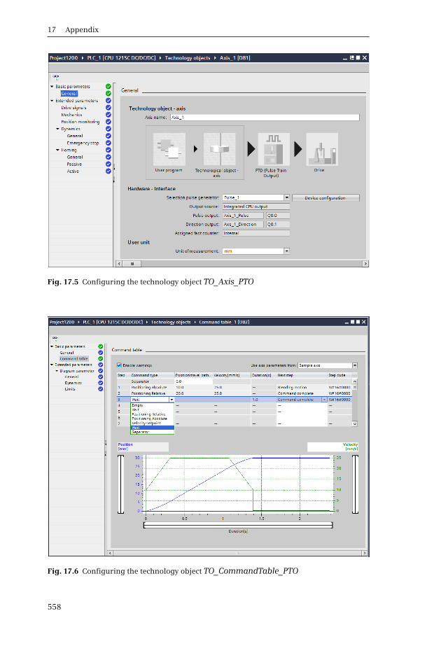
17 Appendix
558
Fig. 17.5 Configuring the technology object TO_Axis_PTO
Fig. 17.6 Configuring the technology object TO_CommandTable_PTO

17.1 Integral and technological functions
559
block whose number you can set. If the Add new and open checkbox is activated,the technology object is opened for configuration. Click OK.
To configure the command table, double-click Configuration in the project treeunder the command table used. In the configuration window, enter the motionprofile (Fig. 17.6).
For a motion sequence, the commands listed in Table 17.4 are available. Either“Complete job” (the axis decelerates to a stop) or “Continue movement” (the axismaintains speed) can be configured as a completion of a positioning command.
The commands in the command table are implemented in the user program withthe statement MC_CommandTable.
Programming the Axis technological axis
You control the Axis technology object and thus the drive with the user programusing the motion control statements. The statements are available in the programelements catalog under Technology and Motion control. To call a statement, drag itwith the mouse into the open block. Each call requires an instance data record,which can be either in a separate block (single instance) or – if the call is made in afunction block – in the instance data block of the calling function block (multi-instance). Fig. 17.7 shows the calls of the motion control statements.
MC_Power enables and disables an axis for motion control.
MC_Reset resets all errors, and acknowledges all errors which can be acknowl-edged.
MC_Home sets a homing point, i.e. the (mechanical) positioning system of the axis is matched with the (logical) coordinate system in the controller.
MC_Halt aborts all movements and stops the axis.
MC_MoveAbsolute starts a positioning motion of the axis to an absolute position.
MC_MoveRelative starts a positioning motion of the axis relative to the start position.
Table 17.4 Commands for the motion control of a axis
Command Action
Positioning Absolute The axis is moved at the configured speed to the specified position.
Positioning Relative The axis is moved the specified distance at the specified speed.
Velocity Setpoint The axis is moved at the specified speed for the specified duration.
Hold The axis is stopped (only after a Velocity Setpoint command).
Wait There is a wait of the specified time between two commands.
Empty This command is used as a placeholder for any other command
Separator This command separates different motion profiles in the command table.

17 Appendix
560
MC_MoveVelocity starts the axis with the defined velocity.
MC_MoveJog starts the axis in jog mode for testing and commissioning.
MC_ChangeDynamic changes the dynamic settings of an axis of motion.
MC_CommandTable implements the commands configured in the commandtable as a motion sequence.
If a motion control statement is still being executed, it must not be interrupted bythe start of the same motion control statement. You should therefore call a motioncontrol statement only once in the user program.
Fig. 17.7 Calling the motion control statements in LAD representation
Calls of the motion control statements
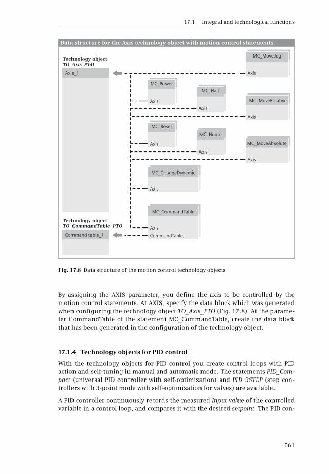
17.1 Integral and technological functions
561
By assigning the AXIS parameter, you define the axis to be controlled by themotion control statements. At AXIS, specify the data block which was generatedwhen configuring the technology object TO_Axis_PTO (Fig. 17.8). At the parame-ter CommandTable of the statement MC_CommandTable, create the data blockthat has been generated in the configuration of the technology object.
17.1.4 Technology objects for PID control
With the technology objects for PID control you create control loops with PIDaction and self-tuning in manual and automatic mode. The statements PID_Com-pact (universal PID controller with self-optimization) and PID_3STEP (step con-trollers with 3-point mode with self-optimization for valves) are available.
A PID controller continuously records the measured Input value of the controlledvariable in a control loop, and compares it with the desired setpoint. The PID con-
Fig. 17.8 Data structure of the motion control technology objects
Data structure for the Axis technology object with motion control statements
Axis_1
Command table_1
Technology objectTO_Axis_PTO
Technology objectTO_CommandTable_PTO
Axis
Axis
Axis
Axis
Axis
Axis
Axis
Axis
CommandTable
Axis
MC_Power
MC_Halt
MC_Reset
MC_MoveJog
MC_Home
MC_MoveAbsolute
MC_ChangeDynamic
MC_CommandTable
MC_MoveRelative

17 Appendix
562
troller calculates a manipulated variable from the difference (the control devia-tion), and this matches the controlled variable to the setpoint.
With a PID controller, the controlled variable comprise three components: theP component which is proportional to the control deviation, the I component whichis calculated by integration, increases along with the duration of the deviation,and finally results in compensation of the deviation, and the D component whichincreases along with the rate of change of the control deviation in order to mini-mize this as rapidly as possible.
The technology object PID_Compact requires an analog input channel for theactual value and an analog output channel for the (analog) manipulated variable.If the manipulated variable is to be output as pulse width modulated signal, a dig-ital output channel is required. The pulse generators integrated in the CPU arenot required.
The technology object PID_3STEP requires an analog input channel for the actualvalue and two digital outputs for “Control up” (e.g. open valve) and “Controldown” (e.g. close valve).
Configuring the PID control technology object
A PID controller can be created in the following ways: You first create a new tech-nology object and then program the controller statement with the specification ofthe technology object as an instance data block, or you first program the control-ler statement, where the required instance data block is the technology object,and then you configure the technology object.
Programming the controller statement
The controller must record the actual value at defined intervals – the scanningtime – in order to be able to determine its time characteristics. Therefore the con-troller statement must be called in a cyclic interrupt organization block whose
Fig. 17.9 Calls of the controller statements in LAD representation
Calls of PID_Compact and PID-3STEP statements
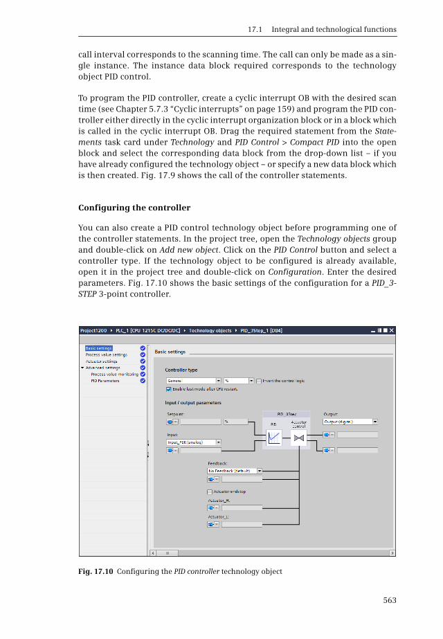
17.1 Integral and technological functions
563
call interval corresponds to the scanning time. The call can only be made as a sin-gle instance. The instance data block required corresponds to the technologyobject PID control.
To program the PID controller, create a cyclic interrupt OB with the desired scantime (see Chapter 5.7.3 “Cyclic interrupts” on page 159) and program the PID con-troller either directly in the cyclic interrupt organization block or in a block whichis called in the cyclic interrupt OB. Drag the required statement from the State-ments task card under Technology and PID Control > Compact PID into the openblock and select the corresponding data block from the drop-down list – if youhave already configured the technology object – or specify a new data block whichis then created. Fig. 17.9 shows the call of the controller statements.
Configuring the controller
You can also create a PID control technology object before programming one ofthe controller statements. In the project tree, open the Technology objects groupand double-click on Add new object. Click on the PID Control button and select acontroller type. If the technology object to be configured is already available,open it in the project tree and double-click on Configuration. Enter the desiredparameters. Fig. 17.10 shows the basic settings of the configuration for a PID_3-STEP 3-point controller.
Fig. 17.10 Configuring the PID controller technology object

17 Appendix
564
17.2 Telephone network connections with TeleService
You use the TeleService to connect a programming device or PC to a PLC or HMIstation via the telephone network. This enables you to manage, control, and mon-itor remote machines or plants from a central point. TeleService is standalonesoftware and does not require the installation of STEP 7. TeleService is includedin the scope of delivery of STEP 7 in the TIA Portal. The connection to the centralprogramming device is established via a modem.
A TS Adapter creates the connection on the station side. The TS Adapter IE Basicconsists of the basic unit and a TS module with the modem or an interface for con-necting to an external modem. The basic unit has an Ethernet interface for connect-ing to a programming device or programmable controller. The TS-Adapter IE Basicis parameterized with TeleService in the TIA Portal. Fig. 17.11 shows the basicstructure of a remote connection using a TS Adapter.
Send an e-mail
The statement TM_MAIL sends an e-mail via the PN interface of the CPU to thedial-in server of the Internet service provider. If there is no direct Internet con-nection via the PN interface, the TS Adapter IE can be used to connect to the phonenetwork. TM_MAIL uses SMTP (Simple Mail Transfer Protocol) as its transfer pro-tocol.
For programming TM_MAIL, drag the statement from the program elements cat-alog under Communication > TeleService to the open block. Fig. 17.12 shows thecall of TM_MAIL in LAD representation.
Fig. 17.11 Controlling a PLC station over a remote connection using TeleService
PG/PC
PG/PC
S
S
PLC station
Industrial Ethernet
Modem
STEP 7 i
COM-/USBconnection
TS adapterIE Basic
Analog, ISDN, GSM
Remote connection with TeleService
S
n TIA portal
Direct connection for assigning adapter parameters

17.3 Telecontrol with CP 1242-7
565
17.3 Telecontrol with CP 1242-7
The telecontrol statements control the connection setup and data transfer with aCP 1242-7 communication module. You will find the communication functions inthe program elements catalog under Communication >Communication processor> GPRSComm:CP1242-7 after the CP 1242-7 communication module has been“subsequently installed” with a hardware support package. The calls of thesefunctions are shown in Fig. 17.13.
Fig. 17.12 Call of TM_MAIL to LAD representation
Fig. 17.13 Calls for telecontrol in LAD representation
TM_MAIL sends an e-mail (SMTP) via an Industrial Ethernet connection. REQ, BUSY, DONE, ERROR, and STATUS control the transmission. The recipient addresses are specified at TO_S and CC. SUBJECT, TEXT, and ATTACHMENT contain the contents of the e-mail. The address of the mail server, the username, the password, and the sender’s address are entered into the instance data.
Calls of TM_MAIL statement
Calls for telecontrol
Establishing a connection via the GSM network
Configure a GPRS module
Terminating a connection via the GSM network
Sending data via the GSM network
Receiving data via the GSM network
17 Appendix
566
Establishing and clearing a connection via the GSM network
TC_CON sets up a communication connection in an S7-1200 station with aCP 1242-7. The connection types ISO-ON-TCP (connection to a CP 1242-7), UDP(connection to any partner), SMS (connection to an SMS client), and telecontrolconnection (connection to a telecontrol server) are available.
The parameters REQ, BUSY, DONE, ERROR, and STATUS control the establishmentof a connection. At the ID parameter, enter the connection ID and at the parame-ter INTERFACE, enter the hardware ID of the CP 1242-7 from the System constantstab in the default tag table. The CONNECT parameter contains a pointer to thedata block with the connection data. Depending on the type of connection used,this data block is derived from one of the system data types TCON_ip_rfc,TCON_IP_V4, TCON_phone, or TCON_WDC.
TC_DISCON closes the connection established with TC_CON. The parameters REQ,BUSY, DONE, ERROR, and STATUS control the establishment of a connection. Atthe ID parameter, enter the connection ID and at the parameter INTERFACE, enterthe hardware ID of the CP 1242-7 from the System constants tab in the default tagtable.
Sending data via the GSM network
TC_SEND sends data via a connection established with TC_CON. The parametersREQ, BUSY, DONE, ERROR, and STATUS control the data transmission. At the IDparameter, enter the connection ID and at the parameter INTERFACE, enter thehardware ID of the CP 1242-7 from the System constants tab in the default tagtable. The DATA parameter contains a pointer to the send data. The number ofbytes to be sent is specified at the LEN parameter.
Receiving data via the GSM network
TC_RECV receives data via a connection established with TC_CON. The parametersEN_R, BUSY, NDR, ERROR, and STATUS control the data transmission. At the IDparameter, enter the connection ID and at the parameter INTERFACE, enter thehardware ID of the CP 1242-7 from the System constants tab in the default tagtable. The DATA parameter contains a pointer to the receive mailbox. You enter themaximum number of bytes to be received at the parameter LEN. The actual num-ber of bytes received is output at the parameter RCVD_LEN.
Transferring configuration data to the CP 1242-7
TC_CONFIG transfers (new) configuration data to the CP 1242-7 communicationmodule and thus overwrites (temporarily) the data configured with the hardwareconfiguration. On the next startup, the initial configuration data is importedagain. The parameters REQ, BUSY, DONE, ERROR, and STATUS control the trans-mission. At the parameter INTERFACE, enter the hardware ID of the CP 1242-7from the System constants tab in the default tag table. The parameter CONFIG con-tains a pointer to a data area with the configuration data whose structure is spec-ified by the system data type IF_CONF.
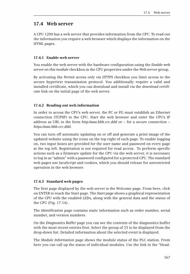
17.4 Web server
567
17.4 Web server
A CPU 1200 has a web server that provides information from the CPU. To read outthe information you require a web browser which displays the information on theHTML pages.
17.4.1 Enable web server
You enable the web server with the hardware configuration using the Enable webserver on this module checkbox in the CPU properties under the Web server group.
By activating the Permit access only via HTTPS checkbox you limit access to thesecure hypertext transmission protocol. You additionally require a valid andinstalled certificate, which you can download and install via the download certifi-cate link on the initial page of the web server.
17.4.2 Reading out web information
In order to access the CPU's web server, the PC or PG must establish an Ethernetconnection (TCP/IP) to the CPU. Start the web browser and enter the CPU's IPaddress as URL in the form http://aaa.bbb.ccc.ddd or – for a secure connection –https://aaa.bbb.ccc.ddd.
You can turn off automatic updating on or off and generate a print image of theupdated website using the icons on the top right of each page. To enable loggingon, two input boxes are provided for the user name and password on every pageat the top left. Registration is not required for read access. To perform specificactions such as a firmware update for the CPU via the web server, it is necessaryto log in as “admin” with a password configured for a protected CPU. The standardweb pages use JavaScript and cookies, which you should release for unrestrictedoperation in the web browser.
17.4.3 Standard web pages
The first page displayed by the web server is the Welcome page. From here, clickon ENTER to reach the Start page. The Start page shows a graphical representationof the CPU with the enabled LEDs, along with the general data and the status ofthe CPU (Fig. 17.14) .
The Identification page contains static information such as order number, serialnumber, and version numbers.
On the Diagnostics Buffer page you can see the contents of the diagnostics bufferwith the most recent entries first. Select the group of 25 to be displayed from thedrop-down list. Detailed information about the selected event is displayed.
The Module Information page shows the module status of the PLC station. Fromhere you can call up the status of individual modules. Use the link in the “Head-
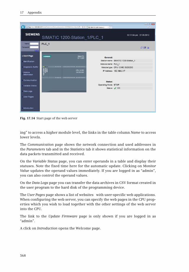
17 Appendix
568
ing” to access a higher module level, the links in the table column Name to accesslower levels.
The Communication page shows the network connection and used addresses inthe Parameters tab and in the Statistics tab it shows statistical information on thedata packets transmitted and received.
On the Variable Status page, you can enter operands in a table and display theirstatuses. Note the fixed time here for the automatic update. Clicking on MonitorValue updates the operand values immediately. If you are logged in as “admin”,you can also control the operand values.
On the Data Logs page you can transfer the data archives in CSV format created inthe user program to the hard disk of the programming device.
The User Pages page shows a list of websites with user-specific web applications.When configuring the web server, you can specify the web pages in the CPU prop-erties which you wish to load together with the other settings of the web serverinto the CPU.
The link to the Update Firmware page is only shown if you are logged in as“admin”.
A click on Introduction opens the Welcome page.
Fig. 17.14 Start page of the web server
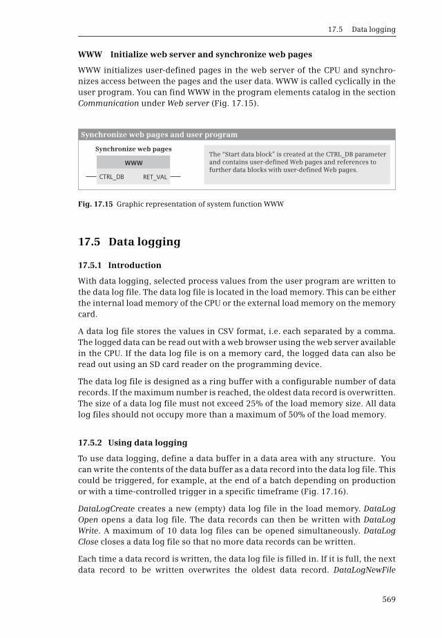
17.5 Data logging
569
WWW Initialize web server and synchronize web pages
WWW initializes user-defined pages in the web server of the CPU and synchro-nizes access between the pages and the user data. WWW is called cyclically in theuser program. You can find WWW in the program elements catalog in the sectionCommunication under Web server (Fig. 17.15).
17.5 Data logging
17.5.1 Introduction
With data logging, selected process values from the user program are written tothe data log file. The data log file is located in the load memory. This can be eitherthe internal load memory of the CPU or the external load memory on the memorycard.
A data log file stores the values in CSV format, i.e. each separated by a comma.The logged data can be read out with a web browser using the web server availablein the CPU. If the data log file is on a memory card, the logged data can also beread out using an SD card reader on the programming device.
The data log file is designed as a ring buffer with a configurable number of datarecords. If the maximum number is reached, the oldest data record is overwritten.The size of a data log file must not exceed 25% of the load memory size. All datalog files should not occupy more than a maximum of 50% of the load memory.
17.5.2 Using data logging
To use data logging, define a data buffer in a data area with any structure. Youcan write the contents of the data buffer as a data record into the data log file. Thiscould be triggered, for example, at the end of a batch depending on productionor with a time-controlled trigger in a specific timeframe (Fig. 17.16).
DataLogCreate creates a new (empty) data log file in the load memory. DataLogOpen opens a data log file. The data records can then be written with DataLogWrite. A maximum of 10 data log files can be opened simultaneously. DataLogClose closes a data log file so that no more data records can be written.
Each time a data record is written, the data log file is filled in. If it is full, the nextdata record to be written overwrites the oldest data record. DataLogNewFile
Fig. 17.15 Graphic representation of system function WWW
WWW
CTRL_DB RET_VAL
The “Start data block” is created at the CTRL_DB parameter and contains user-defined Web pages and references to further data blocks with user-defined Web pages.
Synchronize web pages
Synchronize web pages and user program

17 Appendix
570
allows an “expansion” of the data log file to avoid overwriting old records. Thefunction creates a new (empty) data log file on the basis of the original data logfile.
17.5.3 Functions for data logging
Fig. 17.17 shows the call of functions for data logging in LAD representation.
DataLogCreate creates a new data log file. The parameters REQ, DONE, BUSY,ERROR, and STATUS control the execution of the function. At the NAME parameter,enter the name of the data log file, following the requirements for Windows file
Fig. 17.16 Data structure for data logging
Data structure for data logging
<Name>
<Name>
Data log file
Data log file
Data buffer (= data record)
NAME
ID
HEADER
NAME
RECORDS
DATA
RECORDS
ID
ID
ID
ID
DataLogCreate
DataLogNewFile
DataLogWrite
DataLogClose
DataLogOpen
The data log file is created in the load memory, either in the internal load memory, which is integrated in the CPU, or in the external load memory on the memory card.
DataLogWrite writes the contents of the data buffer as a data record into the data log file.
DataLogNewFile creates a new data log file with the properties of an existing one. The name and the size can vary.
DataLogClose closes a data log file.
DataLogOpen opens a data log file for writing.
DataLogCreate creates a new data log file. DATA specifies the data area of a data record.RECORD specifies how many data records the data log file can accommodate.
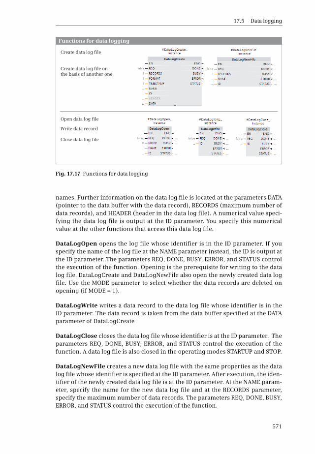
17.5 Data logging
571
names. Further information on the data log file is located at the parameters DATA(pointer to the data buffer with the data record), RECORDS (maximum number ofdata records), and HEADER (header in the data log file). A numerical value speci-fying the data log file is output at the ID parameter. You specify this numericalvalue at the other functions that access this data log file.
DataLogOpen opens the log file whose identifier is in the ID parameter. If youspecify the name of the log file at the NAME parameter instead, the ID is output atthe ID parameter. The parameters REQ, DONE, BUSY, ERROR, and STATUS controlthe execution of the function. Opening is the prerequisite for writing to the datalog file. DataLogCreate and DataLogNewFile also open the newly created data logfile. Use the MODE parameter to select whether the data records are deleted onopening (if MODE = 1).
DataLogWrite writes a data record to the data log file whose identifier is in theID parameter. The data record is taken from the data buffer specified at the DATAparameter of DataLogCreate
DataLogClose closes the data log file whose identifier is at the ID parameter. Theparameters REQ, DONE, BUSY, ERROR, and STATUS control the execution of thefunction. A data log file is also closed in the operating modes STARTUP and STOP.
DataLogNewFile creates a new data log file with the same properties as the datalog file whose identifier is specified at the ID parameter. After execution, the iden-tifier of the newly created data log file is at the ID parameter. At the NAME param-eter, specify the name for the new data log file and at the RECORDS parameter,specify the maximum number of data records. The parameters REQ, DONE, BUSY,ERROR, and STATUS control the execution of the function.
Fig. 17.17 Functions for data logging
Functions for data logging
Create data log file
Close data log file
Write data record
Create data log file on the basis of another one
Open data log file

Index
572
Index
A
ABS 368ACOS 373ADD 367Addressing 85Alarm system (HMI) 528AND (word logic
operation) 392AND function
Description 331with FBD 252with LAD 215with SCL 291
Arc functions 373Area pointer (HMI) 515Arithmetic functions
for numerical valuesDescription 366with FBD 273with LAD 236
for time valuesDescription 369with FBD 273with LAD 236
with SCL 301ARRAY (data type) 104ASIN 373Assignment
Description 334with FBD 259with LAD 222with SCL 294
Assignment list 203ATAN 373ATH 389ATTACH 165Authorization 31
B
Basic Panels 508BCD16 (data type) 95BCD32 (data type) 95
Binary logic operationswith FBD 249with LAD 212with SCL 288
Bit memory 82Block
Calling 137Comparing 432Compile 198Copy protection 132Correct call 200Editing
FBD elements 248LAD elements 211SCL statement 286
InterfaceCorrection 133Description 133Supplying 139
Know-how protection 132Programming
Code block 183Data block 194
Properties 128Block calls
Description 413with FBD 282with LAD 245with SCL 316
Block end functionDescription 412with FBD 282with LAD 244with SCL 316
BOOL (data type) 95BYTE (data type) 95
C
Call structure 204CAN_DINT 158CASE (SCL) 308CEIL 379CHAR (data type) 100CHARS_TO_STRG 387Clock memory bits 84
CommunicationConfiguring 483Open user
communication 484Point-to-point
communication 499Comparison functions
Description 364with FBD 258with LAD 219with SCL 300
Configuring function keys (HMI) 520
Configuring process screen (HMI) 517
Configuring the network 482
Constants table 182Contacts
Comparison 219Edge 218NC contact 213NO contact 212OK contact 219
CONTINUE (SCL) 314Control program
Cycle processing time 439
Programmingwith FBD 246with LAD 209
Control statements (SCL) 307
Controlling the program flowwith FBD 279with LAD 241with SCL 305
CONV 377Conversion functions
Description 376with FBD 275with LAD 238with SCL 299
Copy protection 132COS 373Counter (HSC) 548

Index
573
Cross-reference listfor HMI objects 512for the control
program 201CTD down counter 352CTRL_HSC 552CTRL_PWM 556CTU up counter 351CTUD up-down
counter 353Cycle processing time 437,
439Cycle time monitoring 144Cyclic interrupt 159
D
Data addresses 84Data management
in the CPU 435with STEP 7 29
Data typesClassification 92Elementary 92Structured 101
DATE (data type) 100DEC 369DECO 394DEMUX 395Dependency structure 205DETACH 166Device name, device
number 74DeviceStates 173Diagnostics buffer 437Diagnostics interrupt OB
82 176Digital functions
with FBD 270with LAD 233with SCL 298
DINT (data type) 98DIS_AIRT 166Distributed I/O
AS-Interface 473PROFIBUS DP 462PROFINET IO 456
DIV 367Downloading HMI
program 543DPNRM_DG 471DPRD_DAT 472DPWR_DAT 472DTL (data type) 101DWORD (data type) 95
E
Edge evaluationDescription 338of a binary tag
with FBD 256with LAD 218
of RLOwith FBD 266with LAD 229
with pulse outputwith FBD 261with LAD 224
with SCL 295EN_AIRT 167EN/ENO mechanism
Description 417with FBD 418with LAD 418with SCL 306
Enable peripheral outputs 451
ENCO 395ENO (tag, SCL) 305ErrorStruct (data type) 112Exclusive OR function
Description 333with FBD 254with SCL 292
EXIT (SCL) 316EXP 374Expressions (SCL) 288EXPT 375
F
FILL_BLK 361Filling of bit field
Description 336with FBD 262with LAD 225
FLOOR 380FOR (SCL) 311FRAC 375Function lists (HMI) 528
G
GET_DIAG 175GET_ERROR 170GET_ERROR_ID 170
H
Hardware detection 434Hardware diagnostics 436
High-speed counter 548HMI device wizard 511HMI tags 513HTA 389
I
IEC counter functionsDescription 349with FBD 268with LAD 231with SCL 297
IEC time functionsDescription 344
IEC timer functionswith FBD 267with LAD 230with SCL 296
IF (SCL) 308INC 369Inputs 80INT (data type) 98Interrupt processing
Cyclic interrupt 159Delaying and
enabling 166Introduction 153Process interrupt 163Time-delay interrupt 155
INV 394IP address
Assigning to CPU 424Configuring 73of the programming
device 421
J
JMP_LIST 409Jump distributor
with FBD 281with LAD 244
Jump functionsDescription 406with FBD 280with LAD 242
Jump listwith FBD 281with LAD 243
L
Language setting 207LED (function) 172Library
Editing 42
Index
574
LIMIT 398LN 374Local error handling 169Logic functions
Description 392with FBD 277with LAD 240with SCL 303
LREAL (data type) 98
M
Math functionswith FBD 274with LAD 237
Mathematical functionsDescription 372with SCL 303
MAX 397Memory card 428Memory functions
Description 334with FBD 265with LAD 227with SCL 294
Memory reset 439Memory utilization
online 437, 439MIN 397Minimum cycle time 146MOD 368Modules
Assigning parameters 61Properties 50Status displays 436
ModuleStates 174MOVE 356MOVE_BLK 360MUL 367MUX 395
N
NEG 369Negating result of logic
operationwith FBD 255with LAD 218
Negating the result of logic operationDescription 329with SCL 293
Nesting depthBlocks 125
NORM_X 381
Normally closed contact 213
Normally open contact 212
O
OK testDescription 330with FBD 257with LAD 219
Online tools 439Open user
communication 484Operands 79Operating mode
RUN 119STARTUP 118STOP 118
Operator control and dis-play objects (HMI) 525
Operators (SCL) 286OR (word logic
operation) 392OR function
Description 332with FBD 253with LAD 215with SCL 291
Organization blockCyclic interrupt 159OB 1 main program 143OB 100 startup
program 142OB 80 time error 168OB 82 diagnostics
interrupt 176Process interrupt 163Time-delay interrupt 155
Outputs 80-81
P
Parallel connection 215PEEK (SCL) 90Peripheral inputs 80Peripheral outputs 80-81PLC station
Adding 60Parameterization 61
PLC tag tableEditing 178Monitoring with 445
Point-to-point communication 499
POKE (SCL) 90
Priority classes 154Process image update 143Process interrupt 163PROFIBUS DP
Addressing 465Configuring 467
PROFINET IOAddressing 457Configuring 459Real-Time
Communication 461Program execution
modes 124Program status 441Project
Editing 41Object hierarchy 38
Pulse generator 554
Q
QRY_CINT 161QRY_DINT 158
R
RALRM 473RD_LOC_T 151RD_SYS_T 150RDREC 472RE_TRIGR 145READ_DBL 362REAL (data type) 98Recipes (HMI) 535REPEAT (SCL) 313Resources
Offline 206Retentive behavior 121ROL 392ROR 391ROUND 380RTM 152
S
S_CONV 383SCALE_X 381Scanning of signal state
Description 329with FBD 250with LAD 212with SCL 288
SEL 395Series connection 215SET_CINT 161

Index
575
SET_TIMEZONE 150Setting and resetting
Description 335with FBD 260with LAD 223with SCL 294
Shift functionsDescription 389with FBD 276with LAD 239with SCL 304
SHL 391SHR 389Simulation (HMI) 542SIN 373SINT (data type) 98SQR 374SQRT 374SRT_DINT 158Start-up routine 142STEP 7
Portal view 32Project view 34
STP 147STRG_TO_CHARS 387STRG_VAL 385STRING (data type) 102String functions
Description 398with FBD 278with LAD 240
STRUCT (data type) 104SUB 367SWAP 363SWITCH 410System memory bits 82
T
T branchwith FBD 255with LAD 217
T_ADD 371T_CONFIG 495T_CONV 383T_DIFF 371T_SUB 371
TagsAddressing 85Declaring data tags 198Forcing 452HMI tags 513Introduction 79Modifying 450Monitoring with
Watch tables 449monitoring with
PLC tag table 445PLC tag table 178
TAN 373Technology objects
for motion control 557for PID control 561
TeleService 564Text and graphics lists
(HMI) 526Time
Configuring 148Setting online 151
TIME (data type) 100Time error OB 80 168TIME_OF_DAY (data
type) 101Time-delay interrupt 155TM_MAIL 564TOF off-delay 347TON on-delay 347TONR accumulating ON
delay 348TP pulse generation 346Transfer functions
Description 356with FBD 271with LAD 235with SCL 298
Trigonometric functions 373
Troubleshooting 167TRUNC 380
U
UDINT (data type) 97UFILL_BLK 361
UINT (data type) 97UMOVE_BLK 360User administration
(HMI) 539User data 81User program
Download 425Minimum cycle time 146Process image 143Programming
General 189with FBD 246with LAD 209with SCL 284
Reaction time 146Test with
Program status (LAD, FBD) 442
Program status (SCL) 444
Watch tables 447Troubleshooting 167
USINT (data type) 97
V
VAL_STRG 387VARIANT (parameter
type) 108VOID (parameter type) 109
W
Warm restart 119Watch tables 447Web server 567WHILE (SCL) 312WORD (data type) 95WR_SYS_T 148WRIT_DBL 362WRREC 472WWW 569
X
XOR (word logic operation) 392

www.publicis-books.de
Hans Berger
Automating with SIMATICControllers, Software, Programming, Data Communication, Operator Control and Process Monitoring
5th revised and enlarged edition, 2012, 284 pages, 140 illustrations, 49 tables, hardcover ISBN 978-3-89578-387-6, e 44.90
Hans Berger
Automating with SIMATIC S7-300 inside TIA PortalConfiguring, Programming and Testing with STEP 7 Professional V11
2012, 709 pages, 429 illustrations, 85 tables, hardcover ISBN 978-3-89578-382-1, e 69.90
Hans Berger
Automating with SIMATIC S7-400 inside TIA PortalConfiguring, Programming and Testing with STEP 7 Professional
June 2013, ca. 760 pages, 441 illustrations, 94 tables, hardcover ISBN 978-3-89578-383-8, e 69.90
Nicolai Andler
Tools for Project Management, Workshops and ConsultingA Must-Have Compendium of Essential Tools and Techniques
2nd revised and enlarged edition, 2011, 382 pages, 136 illustrations, 55 tables, hardcover ISBN 978-3-89578-370-8, e 39.90