automating the precision trading system

Automating the Precision Trading System

An Interactive Qualifying Project submitted to the Faculty of

WORCESTER POLYTECHNIC INSTITUTE

in partial fulfillment of the requirements for the

Degree of Bachelor of Science

By

Mihnea Andrei

Yar Zar Moe Htet

Myo Han Latt

With help from:

Michael Radzicki

Hossein Hakim

Date:

5/26/13

Report submitted to:

Professor Michael Radzicki

Worcester Polytechnic Institute

This report represents work of WPI undergraduate students submitted to the faculty as evidence

of a degree requirement. WPI routinely publishes these reports on its web site without editorial

or peer review. For more information about the projects program at WPI, see

http://www.wpi.edu/Academics/Projects.

2

ABSTRACT

The purpose of this project is to scientifically create an automated trading system that

would perform well in different market conditions and that would offer investors the confidence

of trading it. The team used a $400,000 simulated account on the TradeStation platform to

develop and optimize the strategy.

3

Table of Contents

ABSTRACT .................................................................................................................................... 2

Table of Contents ............................................................................................................................ 3

Table of Figures .............................................................................................................................. 8

Table of Tables ............................................................................................................................... 9

CHAPTER 1: SYSTEM OBJECTIVES ....................................................................................... 10

High Winning Percentage ......................................................................................................... 10

High Annual Return .................................................................................................................. 11

Low Draw-Down....................................................................................................................... 12

Robust Across Different Markets .............................................................................................. 12

Low Time Commitment for Trading ......................................................................................... 13

Spends a Big Amount of Time in the Market ........................................................................... 13

Holding Trades over Night ........................................................................................................ 13

CHAPTER 2: FINANCIAL INSTRUMENT TRADED (STOCKS) ........................................... 14

Personal Interest ........................................................................................................................ 14

Liquidity .................................................................................................................................... 15

Tax Implications and Margin Rules set by FINRA................................................................... 16

CHAPTER 3: LITERATURE REVIEW ...................................................................................... 18

Asset Classes: Bonds .................................................................................................................... 18

Options................................................................................................................................... 19

Stocks..................................................................................................................................... 20

Major Stock Exchanges ............................................................................................................. 22

Trading Platforms ...................................................................................................................... 22

TradeStation........................................................................................................................... 23

MetaTrader 5 ......................................................................................................................... 25

Different Types of Trading and Active Investing Systems ....................................................... 26

4

Efficient Market Hypothesis (EMH) ..................................................................................... 26

Dow Theory ........................................................................................................................... 27

CAN SLIM ............................................................................................................................ 29

Capital Asset Pricing Model (CAPM) ................................................................................... 31

Manual Trading vs. Automated Trading ................................................................................... 33

Fundamental Analysis in Stock Trading ................................................................................... 34

Profitability ............................................................................................................................ 35

Management Effectiveness .................................................................................................... 35

Income Statement .................................................................................................................. 36

Balance Sheet ........................................................................................................................ 36

Cash Flow Statement ............................................................................................................. 37

GDP ....................................................................................................................................... 37

Unemployment ...................................................................................................................... 38

Interest Rate ........................................................................................................................... 41

Inflation ................................................................................................................................. 44

Technical Analysis in Stock Trading ........................................................................................ 45

Strategies ................................................................................................................................... 46

Trend Following Strategies ................................................................................................... 46

Support & Resistance Strategies............................................................................................ 47

Volatility Expansion Strategy ................................................................................................ 47

Basic Tools ................................................................................................................................ 48

Trend Lines ............................................................................................................................ 48

Channels ................................................................................................................................ 50

Japanese Candlesticks ............................................................................................................ 52

Fibonacci ............................................................................................................................... 53

Commodity Channel Index (CCI) ......................................................................................... 53

Relative Strength Index (RSI) ............................................................................................... 54

Moving Averages (MA): Simple Moving Average (SMA)&Exponential Moving Average

(EMA) .................................................................................................................................... 55

Random Walk Index (RWI) .................................................................................................. 56

Average True Range (ATR) .................................................................................................. 57

5

Pivot Points ............................................................................................................................ 58

Bollinger Bands ..................................................................................................................... 59

Average Directional Index (ADX) ........................................................................................ 60

Volume .................................................................................................................................. 60

Order Types ............................................................................................................................... 61

Market Orders ........................................................................................................................ 61

Limit Orders .......................................................................................................................... 61

Stop Orders ............................................................................................................................ 62

CHAPTER 4: THE SYSTEM ....................................................................................................... 63

Selecting the “Smoothies” ......................................................................................................... 63

Markov’s Portfolio Optimization Theory ................................................................................. 64

The mean of a Random Variable ........................................................................................... 65

The Variance of a Random Variable ..................................................................................... 65

Introduction to the System ........................................................................................................ 68

Entry and Exit Rules ................................................................................................................. 69

The Basic PTS Strategy ......................................................................................................... 69

PTS with Volume (Version 1) ............................................................................................... 77

PTS with Volume (Version 2) ............................................................................................... 78

PTS with the Relative Strength Indicator (RSI) .................................................................... 78

Mel’s PTS .............................................................................................................................. 79

PTS and the Variations with Simple Moving Average ......................................................... 80

Order Types ............................................................................................................................... 81

CHAPTER 5: THE JOURNEY TO THE BEST COMBINATION ............................................. 82

Results for the Strategies with Volume ..................................................................................... 83

Results for all the Strategy Variations ...................................................................................... 84

Timeframe Analysis .................................................................................................................. 89

Analysis for Different Types of Orders..................................................................................... 91

The Addition of Slippage and Commission .............................................................................. 93

CHAPTER 6: TESTING THE QUALITY AND ROBUSTNESS OF OUR STRATEGY ......... 94

Optimization and Walk-Forward Analysis ............................................................................... 94

Ito’s Lemma ........................................................................................................................... 94

6

Optimized Parameters vs the Initial “Guess” ........................................................................ 96

Walk-Forward Analysis ......................................................................................................... 99

Expectancy, Expectunity and System Quality ........................................................................ 100

CHAPTER 7: SUMMARY & CONCLUSIONS ....................................................................... 102

Recommendations ................................................................................................................... 104

BIBLIOGRAPHY ....................................................................................................................... 105

APPENDIX ................................................................................................................................. 110

Paul King Efficiency Indicator ................................................................................................ 110

Adapted Paul King Efficiency Indicator ................................................................................. 111

Correlation Matrix for the “Smoothies” .................................................................................. 112

MATLAB Code for Portfolio Optimization ........................................................................... 112

Overview of the selected stocks .............................................................................................. 113

The Basic PTS Strategy EasyLanguage code ......................................................................... 114

Strategy that Loads the Net Profit into an ADE ...................................................................... 121

Performance Report for the Strategy before Optimization ..................................................... 123

Valero Energy Corporation (VLO) ...................................................................................... 123

Celgene Corporation (CELG) .............................................................................................. 124

Energy Select Sector SPDR (XLE) ..................................................................................... 125

Google (GOOG) .................................................................................................................. 126

Amazon (AMZN) ................................................................................................................ 127

Toll Brothers (TOL) ............................................................................................................ 128

Walk-Forward Cluster Analysis Results ................................................................................. 129




Google (GOOG) .................................................................................................................. 130

Amazon (AMZN) ................................................................................................................ 131


Equity Curves .......................................................................................................................... 132



7


Google (GOOG) .................................................................................................................. 133

Amazon (AMZN) ................................................................................................................ 134


8

Table of Figures

Figure 1: The “Flash Crash” day ...................................................................................................15

Figure 2: CAPM mathematics formula ..........................................................................................31

Figure 3: Classic test of beta ..........................................................................................................32

Figure 4: The Link between interest rate and the stock market .....................................................42

Figure 5: Naïve (random) diversification .....................................................................................68

Figure 6: View of the chart ............................................................................................................71

Figure 7: Performance report for VLO .......................................................................................123

Figure 8: Performance report for CELG ......................................................................................124

Figure 9: Performance report for XLE ........................................................................................125

Figure 10: Performance report for GOOG ...................................................................................126

Figure 11: Performance report for AMZN ..................................................................................127

Figure 12: Performance report for TOL ......................................................................................128

Figure 13: Walk-Forward analysis for VLO ................................................................................129

Figure 14: Walk-Forward analysis for CELG ............................................................................129

Figure 15: Walk-Forward analysis for XLE ...............................................................................130

Figure 16: Walk-Forward analysis for GOOG ............................................................................130

Figure 17: Walk-Forward analysis for AMZN ...........................................................................131

Figure 18: Walk-Forward analysis for TOL ...............................................................................131

Figure 19: Equity curve for VLO ................................................................................................132

Figure 20: Equity curve for CELG .............................................................................................132

Figure 21: Equity curve for XLE ................................................................................................133

Figure 22: Equity curve for GOOG ............................................................................................133

Figure 23: Equity curve for AMZN ............................................................................................134

Figure 24: Equity curve for TOL ................................................................................................134

9

Table of Tables

Table 1: Ranking for “Smoothies” ................................................................................................64

Table 2: Portfolio weights ..............................................................................................................67

Table 3: Performance for PTS with volume .................................................................................83

Table 4: Performance for the 8 variations on PTS ........................................................................84

Table 5: Sorted performance for the 8 variations on PTS .............................................................87

Table 6: Performance for our best combination ............................................................................89

Table 7: Timeframe analysis ..........................................................................................................90

Table 8: Order type analysis .........................................................................................................91

Table 9: Final combination of strategies .......................................................................................92

Table 10: Performance with slippage and commission .................................................................93

Table 11: Optimization over 3 months’ worth of data ..................................................................96

Table 12: Results for optimized parameters over 1 year worth of data ........................................97

Table 13: Results for initial guess over 1 year worth of data ........................................................98

Table 14: Optimization vs initial guess .........................................................................................98

Table 15: Expectancy, expectunity and SQN ..............................................................................101

Table 16: Correlation matrix .......................................................................................................112

10

CHAPTER 1: SYSTEM OBJECTIVES

High Winning Percentage

Trading a system that has a high winning percentage is important for an investor’s peace

of mind. A system that over a long period of time is profitable, but loses money on most of the

trades is harder to use since, on the short term, it will not offer the investor the confidence to

stick to it.

However, the more analysis, testing and optimization are done, the surer the trader will

be that his/her system will yield profits. Also, a system that has more theoretical concepts and

ideas embedded within it will offer the trader more assurance that, even after taking loosing

trades, profits will show up.

As most automated traders know, it is easier to obtain a high winning percentage on long

positions than it is on short positions. Since the market in the past five years had been in an

overall bearish trend (only in the past year had it start recovering), it has become harder to obtain

automated trading systems that have a high overall winning percentage.

Knowing the economic uncertainty that still threatens the world, we believe that our

system should aim for a high winning percentage on long positions and on short positions.

11

High Annual Return

A high annual return is important for any investor. However, it is also important to know

what the risks associated with a high return are.

In our system, we considered the risk just as important as the return. A system that offers

a high return, but with high risks might be more disadvantageous than one that offers a lower

return, but with a lower risk. An important measure of return to risk in the financial world is the

Sharpe Ratio1.

The Sharpe ratio is defined as:

[ ]

In this formula [ ] stands for the expected value2 of the return on the traded financial

instrument, stands for the risk-free return and stands for the standard deviation3 of the

returns on the traded financial instrument. The risk free rate is considered to be the monthly

return on Treasury Bills. Since those bonds are backed by the U.S. Government, they are

considered to be riskless.

Later in the paper, we will explain in more detail how to find this measure and how we

used it in developing our strategy.

1 “Sharpe Ratio”.Investopedia. < http://www.investopedia.com/terms/s/sharperatio.asp>

2 See page 65 for a short overview of the expected value of a random variable

3 See page 65 for a short overview of the standard deviation and variance of a random variable

12

Low Draw-Down

The draw-down is the peak to trough difference of a system4. Therefore, the draw-down

is the highest loss that a system attains during a given time period.

As with the high winning percentage measure presented earlier, having a low draw-down

is important for the investors’ peace of mind. It is more comfortable to trade a system that has a

low draw-down than one that has a high one.

Our team decided to trade $350,000 of the $400,000, the difference acting as a buffer

zone in case of high draw-downs.

Robust Across Different Markets

Creating an automated trading strategy that is robust across different markets is not an

easy task. Trading systems usually do better in certain markets than in others. As we will see in

the third chapter, there are three types of markets: directionless, trending and volatile. The task of

making a system that is profitable in different markets becomes even harder when we consider

the fact that even stocks within the same sector of the market have different personalities. For

example, it is known among traders that Microsoft is a trending stock, while Netflix is a more

volatile stock. Albeit they both are technology companies, the two trade in completely different

ways.

4 “Drawdown”.Investopedia.<http://www.investopedia.com/terms/d/drawdown.asp>

13

Low Time Commitment for Trading

A low time commitment for trading is one of the advantages of an automated trading

system. These kinds of systems make use of indicators that can detect significant movements in

the market and act accordingly. The trader does not necessarily have to follow the news, albeit

this kind of information can give them an advantage in developing a system that can work better

in the respective economic context.

However, as we will see later in the paper, even with an automated system, the re-

optimization of the parameters after a certain period of time is recommended just because the

general economic conditions can change rapidly, especially when the economy is struggling.

Spends a Big Amount of Time in the Market

Spending a big amount of time in the market has its advantages and disadvantages. For

example, the more a trading system spends time in the market, the higher the risk of that system

will be. However, the more time the system spends in the market, the more likely it is that the

strategy will catch the “big move”. As we will see in the following chapters of this paper, our

team considers that it managed to hedge the risk well and therefore, the possible gains obtained

from spending more time in the market will outrun the downturns.

Holding Trades over Night

A system that holds trades over night is riskier than one that doesn’t since news that is

released during off trading hours can influence the opening minutes. However, as mentioned

above, we believe that we managed to hedge the risk and the strategy itself is not easily

influenced by minor fluctuations in price.

14

CHAPTER 2: FINANCIAL INSTRUMENT TRADED (STOCKS)

Personal Interest

Stocks have been traded by many people through history and one of the most important

questions in the world of finance is to find a model that can accurately predict the stock’s future

price action. As our understanding of the financial world increased, our realization of the

complexity of such a model overwhelmed us. It is not only the inherent complex nature of the

question that attracted us to trade stocks, but also the background that we had.

The future in which we will possibly be able to predict prices with a big certainty is very

far away. The amount of data that we would need is far too big for any computer to process. But

quantifiable information such as financial statements, historical data, option prices, economic

measurements and so on is not the only one that would have to be considered when creating this

model. There is also information that cannot be quantified such as a company’s psychology,

ideals and, more importantly human error and irrational behavior.

An example of how a mistake can trigger a stock market crash is the 2010 “Flash

Crash”5. On May 6

th, a high frequency algorithmic strategy triggered a sell order that was worth

$4.1 billion. The sell order moved the market and triggered other sell orders in other high

frequency algorithms. The end result was that the Dow Jones Industrial Average plummeted 700

points in minutes. How could a model possibly anticipate something like this?

5 Spicer, Jonathan, and Rachelle Younglai. "Single Trade Helped Spark May's Flash Crash." Reuters. Thomson

Reuters, 01 Oct. 2010.< http://www.reuters.com/article/2010/10/02/us-flash-idUSTRE69040W20101002>

15

When it comes to modeling stock prices, even the equation that is used to derive option

prices nowadays, the Black-Scholes partial differential equation, only uses as inputs the risk free

return, the mean and standard deviation of the historical prices and the current price of the

underlying asset.

But even if in the distant future someone would be able to make a very comprehensive

model, all the magic of trading would be lost. Trading wouldn’t be an art as much as it is a

science anymore; it would become solely a science.

Liquidity

Liquidity refers to how easy it is to buy or sell a financial asset6. Therefore, liquidity is

closely related to volume: the higher the volume of a stock, the more liquid it is since it is more

likely to find a buyer/seller in the market. As we will see later in the paper, we chose to trade

6 “Liquidity”.Investopedia. <http://www.investopedia.com/terms/l/liquidity.asp>

Figure 1: The “Flash Crash”

day

16

stocks that have a high volume. This is because, in the case of a trading strategy, a liquid asset

will diminish slippage (the difference between the price at which, according to the system, the

order should have been filled and the price at which it was actually filled7).

Tax Implications and Margin Rules set by FINRA

Trading and strategizing a trading system to achieve optimum returns is just one part of

the puzzle when a person becomes a professional trader in the United States. The other major

parts of the puzzle are the tax implications set by the IRS8 and the margin rules for day trading

set by FINRA9.

In order to be a pattern day-time professional trader, a minimum of $25,000 is needed to

trade as a business. This minimum equity requirement must be deposited into the trader’s

account before any day trading activities are executed. This requirement cannot be satisfied by

cross-guaranteeing with separate accounts. An individual day trading account must meet the

minimum requirement independently. The trader’s account cannot fall below the $25,000

requirement. If the account falls below the set limit, the trader will not be allowed to day trade

until the account is restored to the $25,000 requirement. Additional rules may be applied by the

broker-dealer. They may set higher equity requirement and restrict the buying power to less than

four times the day trading margin excess.

According to FINRA , “a pattern day trader [is] any customer who executes four or more

day trades within five business days, provided that the number of day trades represents more than

7 “Measuring and avoiding slippage”.FUTURES. <http://www.futuresmag.com/2011/08/01/measuring-and-

avoiding-slippage> 8 IRS- Internal Revenue Service

9 FINRA- Financial Industry Regulatory Authority

17

six percent of the customer’s total trades in the margin account for the same five business day

period”. Furthermore, FINRA defines day trade as the buying and selling or selling and buying

of the same security on the same day in a margin account. Here, the definition of security

includes options. If a trader short sells or buys to cover the same security on the same business

day, it is also considered as day trading.

After understanding the regulatory and legal issues, a trader should also be well informed

about the tax implications. Tax implications are the second part of the puzzle that traders have to

solve. Once trading becomes a business for a trader, it would become a major income source for

him/her. And like all other sources of income, people are required to pay taxes. However, tax

implications on trades are significantly different from other types of taxes. In fact, some traders

avoid day-trading in US because the paper work that follows is very complicated. According to

the IRS, “[a] trader must keep detailed records to distinguish the securities held for investment

from the securities in the trading business. The securities held for investment must be identified

as such in the trader's records on the day he or she acquires them.”10

IRS also sets different tax implications for “investors”11

. A detailed description of the tax

code can be found in the investor section of the IRS Tax Top 429: “Dividends, interest from

securities, and gain or loss from the sale of capital assets are not considered proceeds from self-

employment income unless received by a dealer in stocks and securities in the course of their

business.”12

10

“IRS Tax Topic 429” – IRS <http://www.irs.gov/taxtopics/tc429.html> 11

“Investors- typically buy and sell securities and expect income from dividends, interest, or capital appreciation.” 12

“IRS Tax Topic 429” – IRS <http://www.irs.gov/taxtopics/tc429.html>

18

CHAPTER 3: LITERATURE REVIEW

Asset Classes: Bonds

Bonds are a form of debt in which a person loans money to a company, a city, or the gov-

ernment, with the promise that he/she will be paid back in full, with regular interest payments.

For instance, bonds may be sold by a city to raise money to build a bridge, or they may be issued

by the federal government in order to raise revenue to finance its debts13

.

Bonds are generally considered to be safe and they generate a steady flow of income for

the bond holder. For this reason, many investors buy bonds when the stock market becomes too

volatile in order to balance out riskier stock-based investments. However, bonds are far from be-

ing risk-free, and like all other investments, riskier bonds produce higher returns. The first risk of

bonds is whether the bond issuer will make its payments, and thus less credit-worthy issuers pay

a higher yield or interest rate. High-yield bonds are the riskiest and they are generally not very

sought after. On the other hand, there are bonds issued by those with the best histories and these

bonds are deemed to be “investment-grade.” Bonds issued by the U.S. government are known as

Treasuries and they are considered to be the safest and are virtually risk-free. Treasury bonds pay

lower yields than bonds issued by companies that are of investment grade.

How much a bond yields is also determined by how long a person holds the bond. In oth-

er words, the longer a person lends money to the bond issuer, the higher the yield. Thus, bonds

with longer durations, such as 10-year bonds, pay higher yields because the investment is being

tied up for a longer period of time.

13

“What Is a Bond?” The Wall Street Journal Online. Web. 18 May 2013. <http://guides.wsj.com/personal-finance/investing/what-is-a-bond/>.

19

Bond prices are greatly impacted by interest rates; as interest rates rise, bond prices fall.

This is due to the fact that as interest rates climb, new bonds are issued at the higher rate, and this

makes the existing bonds in the market with lower rates less valuable. However, if a bond is

held until maturity, the price fluctuations do not matter. This is because the interest rate was al-

ready set at the time the bond was bought and when the term is up, the bond holder will receive

the face value of the bond back. On the other hand, if a bond is sold on the secondary market be-

fore it reaches maturity, the bond holder could get back less than the original investment depend-

ing on the price of the bond at the time it is sold.

Options

Like a stock or a bond, an option is a versatile security. It is also a binding contract with

strictly defined terms and properties. An option is a contract that gives the buyer a right but not

an obligation to buy or sell an underlying asset at a specific price on or before a certain date14

.

The buyer can choose to let the expiration date go by, at which point the option becomes worth-

less. If this happens, the buyer loses all his investment, which is the money he paid to buy the

option. Options are mere contracts that deal with underlying assets. They are called derivatives

because they derive their value from an underlying asset which is usually a stock or an index.

There are two main types of options, namely calls and puts. A call gives the holder the

right to buy an asset at a certain price within a specific period of time. Calls are similar to having

a long position on a stock because buyers of calls anticipate that the price of a stock will rise

substantially before the option expires. On the other hand, a put gives the holder the right to sell 14

“Options Basics: What Are Options?” Investopedia. Web. 10 May 2011. <http://www.investopedia.com/university/options/option.asp>.

20

an asset within a specific time period. Puts are similar to having a short position on a stock be-

cause buyers of puts hope that the price of the stock will fall before the option expires.

There are four possible positions to hold in the options market. A person may buy or sell

calls or he may buy or sell puts. People who buy options are called holders and those who sell

options are called writers. Options holders are generally said to hold long positions in the market

and writers are said to hold short positions. Holders of either calls or puts have the choice to buy

or sell an asset if they choose to but are not obligated to do so. However, writers of either calls or

puts are obligated to buy or sell. This means that a writer is required to make good on a promise

to buy or sell the underlying asset.

Stocks

A stock is a share in the ownership of a company and it represents a claim on the compa-

ny's assets and earnings. A person who owns a company's stock is one of the many owners or

shareholders of the company and thus, has a claim to everything the company owns. As an own-

er, the stock holder is entitled to his share of the company's earnings as well as any voting rights

attached to the stock. A stock is originally represented by a stock certificate which is a piece of

paper that serves as a proof of ownership. However, today these documents are kept electronical-

ly at the brokerage15

. This makes stocks easier to trade than ever before. Trading can now be

done with the click of a mouse or a phone call, unlike in the past when the certificates had to be

physically taken down to a brokerage in order to be traded.

15

“Stocks Basics: What Are Stocks?” Investopedia. Web. 25 Feb. 2009. <http://www.investopedia.com/university/stocks/stocks1.asp>.

21

Being a stock holder of a public company does not mean that a person has the right to a

say in the daily businesses of the company. Instead, a share comes with the right to cast one vote

to elect the board of directors at annual meetings. In theory, it is the job of the management of

the company to increase the value of the firm for all its shareholders and if it fails to do so the

shareholders have the right to vote to have the management removed. However, in reality, indi-

vidual investors in the markets do not own enough shares to have a material influence on the

company. It is usually the large institutional investors and billionaire entrepreneurs who make

the decisions. The importance of being a shareholder is that a person is entitled to a portion of

the company's profits and has a claim on assets. Profits are sometimes paid out in the form of

dividends and the more shares a person owns, the larger the portion of the profits he will receive.

However, shareholders have a lesser claim on assets than do creditors. If a company goes bank-

rupt and liquidates, shareholders do not get any money until all the banks and bondholders have

been paid out: this is called absolute priority. Therefore, if a company is successful, shareholders

can earn a lot, but if it isn’t they could lose their entire investment. Limited liability is another

very important feature of stocks. Limited liability means that the owner of a stock is not person-

ally liable of any debts the company is unable to pay. Thus owning a stock means that the maxi-

mum value a stock holder can lose is the value of his investment.

The main reason why many companies issue stocks is that they need to raise money at

some point. A company can either take out a loan from a bank or issue bonds (debt financing) or

they can sell part of the company, which is known as issuing stock (equity financing). The first

stock that a private company sells is called the initial public offering (IPO). Issuing stock is gen-

erally more advantageous for companies since they are not required to pay back the money or

make interest payments. Stocks of different companies differ in their own ways. Some compa-

22

nies pay out dividends while many others do not. This is why many people who buy stocks buy

them for their expected appreciation in the open market rather than to gain dividends. Trading

stocks involve large risks but this means a greater return on the investment. Stocks have histori-

cally outperformed other investments such as bonds and savings accounts, and over the long

term an investment in stocks had an average return of about 10-12%.

Major Stock Exchanges

Stock Exchanges are where stocks, bonds, options and futures are traded. In the old days,

stocks were traded in the pit of the stock exchanges but today’s technologies allow people to

trade from personal computers and other devices without having to have an actual broker and a

person in the pit of the stock exchanges. The most renowned stock exchanges are: New York

Stock Exchange (NYSE) in United States, London Stock Exchange in England, Tokyo Stock

Exchange in Japan, and Shanghai Stock Exchange in China. Other stock exchanges, such as

National Association of Securities Dealers Automated Quotation (NASDAQ) and other over-the-

counter (OTC) market are traded electronically. The stock market operates 24 hours a day during

weekdays. Different stock markets operate at different times of the day because of the difference

in time zones.

Trading Platforms

Trading platforms are computer programs and software that traders use to trade. These

trading platforms serve as virtual brokers for traders. There are many kinds of trading platforms

that a trader can use. Different companies, who serve as electronic brokers, provide different

23

kinds of software to their customers. The most discussed and utilized platforms in this paper are

TradeStation and Metatrader 5.

TradeStation

TradeStation is one of the top electronic brokers that specialize in providing the required

data, tools and securities to trade. Using TradeStation, traders can trade stocks, options, futures,

currencies, bonds and mutual funds. It provides various tools and instruments that gives investors

an edge in making the right trades.

TradeStation also provides a trading platform called Tradestation 9.1. This platform

contains charts, stock prices, indicators, strategy components and many other tools which can

provide a potential signal to the trader. The most unique part of TradeStation 9.1 is the ability to

write systems and programs as the trader wishes. These systems or programs can monitor the

price movements of the stock and execute automated orders. Some of these programs can be

used for other purposes than generating automated orders. Manual traders use these systems to

help make decisions on trades.

The programming language that the platform uses is EasyLanguage. EasyLanguage is a

proprietary programming language that was developed by TradeStation. The programming

language can be used to create custom indicators and strategies. The language is originally

created to provide traders without specialized programming knowledge with the ability to create

custom trading strategies. The commands and codes are mostly made up of regular English

words. This allows traders to easily learn the programming language. Other programming

languages are more complex and time consuming to learn compared to EasyLanguage.

24

TradeStation 9.1 also offers pre-made programs. There are six general types of programs

that TradeStation provides: Indicator, ShowMe, PaintBar, ActivityBar, ProbabilityMap and

Strategy. Indicators are technical indicators that are placed on price charts of stocks. ShowMe

and PaintBar are other forms of indicators. A ShowMe alerts the trader by placing a point on the

chart when the predefined conditions of the programs are met and a PaintBar fills the bars of the

chart with a predefined color that is set in the program in order to indicate that the defined

conditions are met. An ActivityBar displays all the price actions that occurred within each bar on

the chart. This allows the trader to observe the price movement in a more precise manner. A

ProbabilityMap allows the trader to view potential price changes using probability calculations

derived from the recent trading histories16

. ProbabilityMaps are generally used for forecasting

future price changes. Strategies are similar to technical indicators except traders include buy and

sell orders in the system.

TradeStation 9.1 also provides other features such as backtesting with historical data.

Backtesting analysis is one of the essential analyses that traders are recommended to perform

before the system is utilized in the actual market. TradeStation 9.1 allows traders to backtest not

only on the past year’s data but also on data several years old. TradeStation can also run other

types of analysis, for example, the walk forward optimization.

16

“About ProbabilityMap Studies.” TradeStation. Tues, 23 Apr 2013. <http://help.tradestation.com/09_01/tradestationhelp/pm/about_pm_studies.htm>

25

MetaTrader 5

MetaTrader 5 is another type of popular trading platform that traders use to trade.

MetaTrader 5 is the next version from MetaTrader 4. The Platform has been added with more

and newer features that enhance the performance of the platform. The MetaTrader platform has

similar capabilities to the TradeStation platform. It can also perform various functions such as

creating indicators, buy and sell orders and other similar functions as TradeStation’s.

MetaTrader is different from TradeStation because the platform uses a different

programming language. It uses MetaQuotes Language (MQL) and because it is version 5, it is

called MQL5. This programming language is similar to that of the C programming language

which is the most widely used programming language. Since MetaTrader 5 uses a more complex

programming language, there are fewer limitations to the complexity of the system which the

trader can create.

MetaTrader has three general types of programs: scripts, custom indicators and expert

advisors. Scripts are the simple programs that are intended to run a simple task once. This task

would be such as a buy and sell order according to a simple strategy. Custom indicators are

indicators that are intended for graphical display of calculated parameters. Expert advisors are

fully functioning trading systems that execute trades automatically.

26

Different Types of Trading and Active Investing Systems

After understanding the available resources and the details of the asset classes and

where/how they are traded, a trader should now get familiarized with different trading theories.

By understanding these theories, traders can further develop more complex systems. The four

different kinds of theories which will be discussed in this section are: Dow Theory, CANSLIM,

Efficient Market Hypothesis and Capital Asset Pricing Model.

Efficient Market Hypothesis (EMH)

The Efficient Market Hypothesis (EMH) is an early 1990’s capital market theory that

states that in a liquid market, security prices fully reflect all available information at any given

time and thus it is impossible to beat the market. The EMH exists in three degrees, namely the

weak, semi-strong, and strong, each pertaining to the degree of public and private information

the theory assumes is factored into the price of stocks17

.

The assumptions of the weak form of EMH are that all available security market infor-

mation is fully reflected in the current prices of stocks and that the future direction of security

prices is not affected by the past price and volume data. It states that excess returns are impossi-

ble to be achieved using technical analysis.

The semi-strong form of EMH assumes that the release of all new public information is

rapidly adjusted into the current stock prices and that available market and non-market public

17

“Efficient Market Hypothesis.” Morningstar Investing Glossary. Web. <http://www.morningstar.com/InvGlossary/efficient_market_hypothesis_definition_what_is.aspx>.

27

information have been factored into security prices. It states that excess returns cannot be

achieved using fundamental analysis.

The strong form of EMH deals with the assumptions that all public and private infor-

mation are fully reflected in the current stock prices, security prices have factored into them all

market, non-market, and inside information, and that there is no such thing as a monopolistic ac-

cess to relevant information. It assumes a perfect market and states that it is impossible to con-

sistently achieve excess returns.

Dow Theory

Dow Theory was originally derived from a series of Wall Street Journal editorials written

by Charles H Dow18

. It has been developed further by other people and the complete theory is

published by his followers. Dow Theory states that the market is in an upward trend when one of

its averages (industrial, or transportation) advances above a previous important high and is

accompanied by a similar advance in the other average19

.

When understanding Dow Theory, there are six basic tenets that the trader should

understand. The first tenet of Dow Theory is that the stock market reflects all news and available

information, such as past, present or future information. Information of different aspects reflects

the prices of stocks. For example, news of the resignation of a particular company’s CEO can

trigger the stock price of the company to fluctuate violently or mildly depending on the

expectations the market has for the new CEO.

18

“Dow Theory: Introduction.” Investopedia. Wed, 25 Feb 2009. <http://www.investopedia.com/university/dowtheory/> 19

“Dow Theory.” Investopedia. Sun, 15 Feb 2009. <http://www.investopedia.com/terms/d/dowtheory.asp>

28

The second tenet of Dow Theory is that the trader should be aware that the market has

three types of movement. The first type of movement is the “main movement” or major trend

which lasts from less than a year to several years. The second type of movement is the “medium

swing” where 30% to 60% of the primary price changes occur. The secondary movement may

last from a few days to a few months. The third movement is called “short swing” or subtle

movement caused by the traders’ difference in opinion. It lasts from hours to a few weeks. All of

these movements can occur simultaneously.

The third tenet of Dow Theory is that major market trends have three phases to it. The

accumulation phase is the earliest phase of market trends where traders, with a specific

knowledge about the stock, are actively purchasing shares against general market opinion. The

price of the stock does not change rapidly because these traders are buying the stock when there

is supply in the market. When trend followers and other professional traders participate, the

market trend shifts to Phase 2. During Phase 2, rapid price movement occurs due to increasing

demand from the traders. Phase 3 occurs when the whole market realize the market trend and

early-bird traders begin to sell their holdings.

Dow Theory states that a shift from bull to bear market cannot be a signal unless market

indexes are in agreement20

. If the indexes are not in agreement, it is hard to predict a new trend.

Dow Theory can also be affected by the stock market’s and the business’ condition. In order for

stock market to perform well, the actual business condition has to be good as well.

Volume is the second most watched indicator that technical traders use, after price

movements. Dow Theory states that volume should increase when prices and the trend move in

20

“Market Indexes Must Confirm Each Other.” Investopedia. Wed, 25 Feb 2009. <http://www.investopedia.com/university/dowtheory/dowtheory4.asp>

29

the same direction and decrease when prices and trend move in opposite directions21

. A large

volume in the trending market usually confirms that the existing trend is strong. If the volume is

decreasing in an upward trend, the existing trend is weak. Hence, a higher percentage of winning

trades can be achieved by studying not only the trend, but also the volume.

The sixth tenet to Dow Theory is that trends exist even if there is market noise in the

current trend. This means that even though market may temporarily move in the opposite

direction to the trend, the market will resume to its initial state. The determination of the reversal

of the trend or the temporary movement in initial trend is not an easy task. There is no specific

way to determining whether there is a temporary opposite movement or a reversal to the trend.

CAN SLIM

CAN SLIM is another type of theory that is important to be familiarized with when a

person is learning to trade. CAN SLIM is developed by William J. O’Neil who was the co-

founder of Investor’s Business Daily. The point of the strategy is to isolate leading stocks that

have the potential to achieve high gains in the near future. CAN SLIM is an acronym that stands

for its various components.22

The letter C stands for current earnings. Current earnings are associated with earnings per

share of the company. EPS is a measure of a company’s profit. The bottom-line is that if the EPS

of a publically traded company increases, the stock satisfies the C component. However, CAN

21

“Volume must confirm the trend.” Investopedia. Wed, 25 Feb 2009. <http://www.investopedia.com/university/dowtheory/dowtheory5.asp> 22

“Stock-Picking Strategies: CAN SLIM”.Investopedia. <http://www.investopedia.com/university/stockpicking/stockpicking7.asp>

30

SLIM follows a stringent way of identifying stocks. The company’s EPS in the most recent

quarter must have grown yearly. The growth should be at least 18%.

The letter A stands for annual earnings and it is another important quantitative analysis

similar to that of current earnings. The growth of annual earnings should be above 25% for the

past 5 years.

The letter N stands for new products or services. CAN SLIM also focuses on the

anticipation of future growth of the company. The company should promise potential growth in

order to maintain the stock’s increasing price.

The letter S stands for supply and demand. Supply and demand are the basic principles of

economics and they are utilized in this theory. The theory follows that a smaller institution would

have a smaller amount of outstanding shares than larger institutions have and thus, it would have

a limited amount of shares and limited supply. Hence, the price increases.

The letter L stands for leader or laggard. CAN SLIM also examines the market leaders

and market laggards by comparing the relative price strength of the stocks. The score can range

from 1-99; a score of 99 means that the company outperformed 99% of the stocks in its

respective market group. CAN SLIM recommends stocks with a score of 70 or more.

The letter I stands for institutional sponsorship. CAN SLIM require that some of the

company’s shares should have been owned by mutual funds in the most recent quarter.

The letter M stands for market indexes. The particular stock must follow the general

market indexes such as Dow Jones Industries, S&P 500, etc.

31

In a nutshell, if all of these components are used in the picking of a stock to trade, the

trader is using a CAN SLIM strategy to trade. Despite its unique analysis of the components, the

strategy lacks the exit from the market. This is why traders also use different theories to form a

unique system for their own use.

Capital Asset Pricing Model (CAPM)

Capital Asset Pricing Model (CAPM) is another theory that is used in trading stocks. This

theory is more concerned with financing the trades and the investments. CAPM was originally

developed by William Sharpe, who was a financial economist and a Nobel laureate. The model

describes the relationship between risk and expected return, which is used in the pricing of secu-

rities23

. There are two different types of risks: Systematic risks (undiversifiable risks) and unsys-

tematic risks (diversifiable risks).A systematic risk is an uncontrollable risk that traders must

take, such as the rate of interest and inflation. An unsystematic risk is the risk associated with a

specific stock that can be eliminated by diversifying the trader’s portfolio.

The model has the following formula:

The basic idea to this formula is that it takes into account two components: time value of

money and risk. Time value of money is embedded in the factor and risk is embedded in the

23

“Capital Asset Pricing Model – CAPM”.Investopedia. <http://www.investopedia.com/terms/c/capm.asp>

Figure 2: CAPM mathematical formula

32

risk measure, beta, which compares the returns on the asset to the returns on the market, to time

and to risk premium. The risk premium is the expected return from the market minus the risk

free rate of return.

Beta is a coefficient that Sharpe has developed to measure the risk of a stock. It is a

measure of the relative volatility of a stock (i.e. the fluctuation of prices). Beta is originated from

a statistical analysis that compares the return of a particular stock to the market return in the

same period of time.

A linear relationship between the monthly returns and the beta of a stock shows that a

riskier investment should earn a premium over the risk free rate24

.

The bottom line of the model is that a stock with a high rate of return is due to the risk

factor of the stock. The model states that, in general, the higher the risk of the stock, the larger

the rate of return of the stock.

24

“The Capital Asset Pricing Model: An Overview”. Investopedia. <http://www.investopedia.com/articles/06/capm.asp>

Figure 3: Classic test of beta

33

Manual Trading vs. Automated Trading

There are two main ways to trade in a stock market: manual trading and automated

trading. The main reason why there are two different ways is because traders may use different

forms of analysis to trade. In general, manual traders use fundamental analysis while automated

traders use technical analysis. The type of trading a trader chooses to trade also depends on

personal preferences.

Manual trading is a traditional trading method that investors have used since trading days

have begun. Manual trading involves human judgment and decision-making. These investors use

fundamental analysis of a stock by studying the condition of the economy and performance of

the companies. They also make their decisions based on news and media. This method is time

consuming and stressful. The fundamental analysis in manual trading involves the analysis of

macro factors such as GDP, interest rate, unemployment and inflation rate, and of micro factors

such as financial statements and balance sheets. In a way, manual traders are investing rather

than simply trading.

Despite the fact that manual trading involves fundamental analysis, this method has a big

disadvantage compared to automated trading: the psychological state of the trader. Since manual

trading involves the use of human decision-making, the trading method can be compromised by

the psychological states in which a trader might be. Manual trading is a good and safe method to

trade if a trader follows his/her set of rules stringently. The downfall of manual trading occurs

when the trader deviates from the proposed set of rules due to the psychological pressure from

market conditions.

34

Fundamental Analysis in Stock Trading

The fundamental analysis of the stock market is determined by many economic and

political variables which are responsible for the swings in the prices of the stocks. On top of

these variables, the market is also affected by the traders’ psychological factor, which can move

the stocks’ price. Sometimes, the price would not increase above a certain level due to the

expectations and the psychology that traders have.

The economic variables’ effects can be both on macro and micro levels. The fundamental

analysis of the stock market that is involved on the micro level would be the performance of the

individual company and the overall performance of the industry itself. Since stock markets are

affected by the performances of a whole set of economic factors, predicting the price of the stock

is quite difficult. Nevertheless, using the right indictors and following a set of rules when trading

stocks can reduce the risk of loss and increase the chances of predicting the direction of the price.

The market analysis techniques are the ones that reduce the risks in the investment and that

determine a better position sizing strategy.

When it comes to measuring the performance of a company, the most commonly used

factors can be classified into four main categories: profitability, management effectiveness,

income statement, and balance sheet and cash flow statement25

.

25

“Key Statistics”. Yahoo Finance. <http://finance.yahoo.com/q/ks?s=AMZN+Key+Statistics>

35

Profitability

As the name implies this measure quantifies the profit of a company. The two key

statistics in this case are the profit margin and the operating margin.

The profit margin measures how much the company keeps as earnings from each dollar

that it makes in sales 26

. The formula used for computing this measure is:

Meanwhile, the operating profit margin measures the portion of a company’s sales that is

left over after paying for variable costs of production such as wages, raw materials, interest on

debt, etc. 27

Management Effectiveness

When it comes to the statistics that measure how effective the management is at using its

assets to generate earnings, there are, again, two key measures: return on assets (ROA) and

return on equity (ROE).

ROA measures how profitable a company is relative to its assets28

:

In the same way, ROE measures how profitable a company is with respect to its

shareholders’ equity:

26

“Profit Margin”.Investopedia.<http://www.investopedia.com/terms/p/profitmargin.asp> 27

“Operating Margin”.Investopedia.<http://www.investopedia.com/terms/o/operatingmargin.asp> 28

“Return on Assets-ROA”.Investopedia.<http://www.investopedia.com/terms/r/returnonassets.asp>

36

Income Statement

The income statement of a company that is listed on a stock exchange also provides some

insight into the company’s performance. Some of the most important figures that traders use are:

revenue, gross profit and EBITDA.

Revenue is the amount of money that a company receives from selling its products and

services 29

:

Gross profit is derived using the revenue. It is the remaining profit after deducting the

cost of producing a good or providing a service 30

.

Finally, EBITDA is income that takes into account interest, taxes, depreciation and

amortization 31

:

Balance Sheet

On the balance sheet the measures of most interest are the total cash and the total debt

that a company has. Those measures are used to compute other ratios such as the debt-equity

29

“Revenue”.Investopedia.<http://www.investopedia.com/terms/r/revenue.asp> 30

“Gross Profit”.Investopedia.<http://www.investopedia.com/terms/g/grossprofit.asp> 31

“Earnings before Interest, Taxes, Depreciation and Amortization-EBITDA”.Investopedia. <http://www.investopedia.com/terms/e/ebitda.asp>

37

ratio and, more importantly, the price-earnings ratio32

. The latter one is computed using the

following formula:

Cash Flow Statement

The most important measure in this case is the operating cash flow (OCF). This statistic

is important because it reflects whether or not the company will need external financing in order

to maintain its operations. It is calculated using the adjusted net income for depreciation, changes

to accounts receivable and changes in inventory.

Besides measuring the performance of a company, measuring the performance of the

economy is also important. Some key statistics when it comes to the macro level of the

fundamental analysis are: GDP, unemployment, interest rate and inflation.

Gross Domestic Product (GDP)

The big picture that most traders should pay attention to is the GDP of the economy. It

does not matter which country the trader trades in, the GDP of the country where a particular

trader is trading should be analyzed. GDP is the commonly used index to measure the strength of

an economy. GDP is calculated using the country's expenditure on consumer spending,

entrepreneurial investments, government spending and the net exports in a given period of time;

yearly and quarterly are most commonly used. The growth of the GDP indicates that the

32

“Price-Earnings Ratio – P/E Ratio”.Investopedia. <http://www.investopedia.com/terms/p/price- earningsratio.asp>

38

economy is growing. An increase of 3% would be a normal growth rate. A higher rate of growth

than 3% can put the economy in negative circumstances such as inflation. Inflation indicates that

the growth of the economy is slowing down and the prices of the goods and services are rising,

with the purchasing power of the people declining.

A decrease in GDP would indicate that the economy is shrinking. Consecutive quarters

with a negative growth are considered to lead to recession. During a recession, the economy of a

particular country faces hardship. People would lose their jobs as employers cut their company’s

workforce. Stocks, currencies and other assets’ value depreciate as the economy suffers from

recession. The trading activities for assets slow down dramatically.

Unemployment

The unemployment rate of a nation is another macroeconomic variable that affects the

swings in the prices of the stocks. Unemployment is, usually, considered as one of the factors

that determine the strength of the economy. “Unemployment rate is the percentage of the total

labor force that is unemployed but actively seeking employment and willing to work”33

.

Unemployment rate is negatively correlated to the strength of the economy. When the economy

is strong and rising, the unemployment rate is low, and when the economy is weak, the

unemployment rate is high. The desired normal rate of unemployment in an economy is about 4-

5%. When an economy recovers from recession, the unemployment rate usually tends to fall.

This fall in unemployment indicates that the economy is gaining strength, thus the prices of the

stocks would increase as well. Therefore, stock traders pay great attention to this measure.

33

“Unemployment Rate.” Investopedia. <http://www.investopedia.com/terms/u/unemploymentrate.asp>

39

Unemployment exists in many different forms. The natural rate of unemployment is the

general unemployment that exists in the economy due to imperfect information and job

shopping34

. This form of unemployment rate is the expected unemployment rate when the

economy is in full capacity. Usually people that are between jobs make up the large portion of

the natural rate of unemployment. This is the desired unemployment rate which has been

discussed earlier: 5%. An economy that is in a dynamic state would have a small unemployment

rate.

The next form of unemployment is structural unemployment. Structural unemployment

occurs when the market economy changes its demand for certain skills which are often replaced

by technology or other factors35

. This can be due to the fact that many workers do not require the

correct skills set for the job or they might not be in the right part of the country where the jobs

are available for them. A classic example of the rise in structural unemployment would be that of

the 1990's, when the demand for workers with computer skills rose during the tech bubble.

Structural unemployment is also considered to be permanent unemployment which can be only

improved by learning new skills that are demanded by the market. Although structural

unemployment is considered to be a dangerous factor for the economy, traders are not too

concerned with this because structural unemployment usually turns into seasonal unemployment.

This latter type of unemployment is due to seasonal changes and to a lack of demand during a

certain time of the year. Usually the construction industries are affected by the weather changes,

34

“Natural Rate of Unemployment” Macroeconomics – Types of Unemployment. Wed, 18 Feb 2009. <http://www.investopedia.com/exam-guide/cfa-level-1/macroeconomics/unemployment.asp> 35

“Macroeconomics - Types of Unemployment”. Wed, 18 Feb 2009. <http://www.investopedia.com/exam- guide/cfa-level-1/macroeconomics/unemployment.asp>

40

thus creating seasonal unemployment. Therefore traders who are trading construction materials

and construction stocks should be aware of this kind of unemployment.

Fictional unemployment is a type of unemployment that occurs when workers are

voluntarily between jobs. This temporary unemployment may exist when people search for new

jobs in hopes of finding a better job than the previous one or just voluntarily change jobs due to

their change in preferences.

Cyclical unemployment is the type of unemployment that traders should pay attention to

the most. This type of unemployment occurs when the economy faces recession and when the

overall business activity in the market declines. During a recessionary period, traders should pay

close attention to the rate of cyclical unemployment because many other traders will also be

concerned with this measure. As the economy recovers from the recessionary period, the

unemployment rate falls and investors’ and traders’ confidence would rise as well, which, in

turn, would increase the prices of stocks. A good trader would not miss the opportunity to ride

along with the momentum of the market.

Unemployment data and jobless claims are released on a weekly basis, each Thursday.

They can be obtained from checking economic calendars such as the Bloomberg Economic

Calendar. These calendars inform traders the predicted numbers and the actual numbers, and the

stock market reacts to these numbers. If the actual number of jobless claims is less than the

predicted number, typically, it can be speculated that the price of the stock would rise.

41

Interest Rate

Interest rate is perhaps the most important macroeconomics factor that influences the

stocks’ swings in prices. Interest rate is the key factor that governs where the capital should be

invested. Depending on the rate of interest, an investor may or may not invest in stocks. Interest

rate is the rate at which the banks borrow money to the borrower. In the United States, the rate of

interest is indirectly governed by the Fed’s Federal Fund’s Rate and by the overnight rate. The

overnight rate is the interest rate at which a depository institution lends immediately available

funds to another depository institution overnight to meet the reserve requirement that is set by

the central banks36

. The overnight rate has many other derivative functions in the economy. By

setting the overnight rate, the central banks can indirectly control the money in the economy. By

controlling the money supply, the inflation rate of the economy can be controlled.

Why should investors be concerned with the federal funds rate? Investors should pay

attention to the federal funds rate because it has an indirect effect on the stock market. A change

in the federal funds rate has a ripple effect on the economy as a whole. For example, if the

federal funds rate is increased, the first indirect effect on the economy will be that it will be more

expensive for individuals and businesses to borrow money from the banks. If the individuals

cannot spend as much as they could in the past, the economy will slow down which will affect

the businesses’ profits and revenues. The businesses are also affected in another way. They also

borrow money from banks to operate and expand their operations. When the rate of interest is

high, companies will try to avoid borrowing money. Thus the growth of the company can slow

down which, again, can result in a decrease in profits.

36

“Overnight Rate.” Investopedia. Sun, 15 Feb. 2009. <http://www.investopedia.com/terms/o/overnightrate.asp>

42

But how do stock prices react to the federal funds rate? Stock prices are affected through

the performance of the company and the value of the companies. One way to measure the value

of the company is to take the sum of the expected future cash flow, which will be discounted for

present value, and divide it by the number of shares available37

. This calculation is based on the

expectations that investors have and, thus, the price fluctuates because of the different

expectations that different people have. Based on these differences, investors are willing to sell

or buy shares at different prices. If the growth of the company is slowed down or cut back due to

an increase in the borrowing interest rate, then the investors’ expectations of future cash flow

will be less. All being constant, this will cause the prices of the stocks to fall. If many other

companies in the market experience this effect, this can result in a fall of the indexes as a whole.

Figure 4: The Link between interest rate and the stock market38

37

“How Interest Rates Affect the Stock Market.” Investopedia. Sun, 07 Oct 2012. <http://www.investopedia.com/articles/06/interestaffectsmarket.asp> 38

“Stock Shastra #29: Learn to read the signals of interest rate and its impact on stock market.” Stockshastra. <http://stockshastra.moneyworks4me.com/basics-of-investing/stock-shastra-29-learn-to-read-the- signals-of-interest-rate-and-its-impact-on-stock-market/>

43

When the stock market is in bearish due to a high interest rate, investors should avoid

placing their capital in sectors like real estates, automobiles and capital intensive industries. This

is because these sectors are most affected by a high interest rate. A sector that would have a

small positive effect from a high interest rate would be the banking sector. Their profit can rise

from the high interest rate if some businesses are still required to borrow money despite the

increased interest rate.

The bottom line is that the rate of interest has many effects on the economy. The central

bank uses it as a monetary tool to control the inflation rate in the economy. This limits the

amount of investment in the economy due to a high interest when borrowing. Individuals’ and

businesses’ expenditures are lessened, thus the companies’ growth rate slows down, which lastly

affects the stock prices. Therefore, interest rate is generally negatively correlated to stock prices.

Another reason why investors should be aware of a rise in the federal funds/interest rate

is because government securities have strong ties to the federal funds rates. Federal funds rate

has positive correlation with 10 years Treasury bonds and it is considered as a safe haven when

the interest rate is high. This investment is more desirable than investing in stock when the

interest rate is high because it is considered risk-free. For most investors, the sum of the risk-free

rate and the risk premium is the desired return for investing in stocks. Different investors have

different tolerances for risk premium. Risk premium is the return in excess of the risk-free rate of

return that an investment is expected to yield39

. Generally, the total required return increases as

the risk-free rate goes up. Thus interest rate plays a major role in the investment of the businesses

and to the people investing in the stock market.

39

“Risk Premium.” Investopedia. Sun, 15 Feb 2009. <www.investopedia.com/terms/r/riskpremium.asp>

44

Inflation

Inflation is another fundamental indicator that affects the fundamental analysis of stocks.

Inflation is the measure of the change in prices over time. The general level of prices of goods

and services increases when the inflation rises and the prices decrease when the inflation falls. In

general, the rise in inflation is negatively related to the amount of investment made by

businesses. Therefore it is not favorable to have a high inflation when purchasing stocks.

Inflation causes the investors to pay more for a stock even though the actual value of the stock is

less.

Inflation tends to increase as the economy expends and jobs are created. Due to this

effect, many analysts and traders are wary of inflation in the economy because they fear that the

expansion of the economy might not be the actual representation of the economy but rather

reflecting an inflationary boom40

. In an inflated market, goods and services are overpriced due to

the decrease in value of its currency. The value of currency is decreased because more money is

added to the economy for the same amount of resources that is being traded in the market.

The Fed is also especially wary when inflation rises. Inflation is controlled by the Fed’s

short-term interest rate. The interest rate is increased when inflation rises because the Central

Bank is responsible for controlling the inflationary boom. As it has been mentioned in the

interest rate topic, the interest rate is negatively related to stock trading and investment. So a high

inflation can cause the interest rate to get higher which, in return, would slow down the trading

of stocks.

40

“Inflation’s effect on the Stock Market: Why Good News is Bad News on Wall Street.” Investment U. <http://www.investmentu.com/2006/February/impact-of-inflation-on-stock-market.html.>

45

Inflation is measured through price indexes such as consumer price index and producer

price index. Consumer price index is the change in the price of basket of goods and services.

These can be gasoline, food, clothing and other products that the typical household buys on a day

to day basis. The rate of inflation can be calculated though using different indexes. For example,

The targeted inflation rate for most economies is between 2% and 3%. However a

negative inflation or a deflation is not considered a favorable condition to be in. In fact, a

deflation is considered worse than a creeping inflation because deflation indicates that the

economy will be shrinking. Why would someone buy something this year if next year the prices,

on average, will decrease?

Technical Analysis in Stock Trading

The technical analysis in stock trading differs from the fundamental one in that it is

mainly focused on the movements in stock’s price. Those movements can be predicted by using

different strategies and indicators. Some of those technical analysis ideas will be presented later

in the chapter and some of them were also used in developing our strategy.

46

Strategies

As we mentioned earlier in the paper, there are three main types of markets41

(trending,

directionless and volatile), each one having different types of trading systems that, in general,

seem to work the best for them.

Trend Following Strategies

Before we delve into what the characteristics of a trending strategy are, we need to

understand what a trending market is. Such a market can be characterized in many different

ways, but a common definition would be that it has higher highs and higher lows.

A strategy that would perform well in those markets should never miss the big move. The

easiest way to accomplish this is to be in the market all the time. If the strategy is always in the

market, it will never miss an important trend.

Another characteristic of a trend following system should be to have a stop order above

or below the current price that would act as a confirmation for the trend. For example, if the

strategy predicts an uptrend and you have a stop order above the current price and, moreover, in

the case in which the price indeed goes above the stop price, the order will be filled. If the price

falls below the set stop price, the order will not be filled.

The last important characteristic is that the devised strategy should be able to limit losses

when the market is not moving in any particular direction. This is because a trend following

system can incur big draw downs in those situations.

41

Wright, C. (n.d.). Trading as a Business.

47

Support & Resistance Strategies

Support and resistance strategies try to make profit from the price swings in directionless

markets. Since the market doesn’t show any particular direction 85% of the time, the winning

percentage of those kinds of strategies is higher. Therefore, they are also psychologically easier

to trade.

However, a major disadvantage is that those strategies will miss the big move. This is

because of the way they are inherently designed to work: buy low and sell high. When the stock

becomes increasingly overbought, the strategy looks to get out. Another disadvantage is that the

slippage and commission will be greater than those of a trending strategy because of the high

number of trades that are generated.

Volatility Expansion Strategy

A volatile market is characterized by big jumps in the stock’s price. A strategy that is

profitable in those conditions looks precisely for finding those gaps. Such a strategy is in the

market for a small amount of time. Albeit the winning percentages for those type of systems is

even bigger than for the ones generated by a support and resistance one, the number of trades is

also bigger. This, in turn, generates even higher slippage and commission costs.

Now that we have covered the three main types of strategies, we are ready to move on to

the next section in which we will present the different types of tools used to predict the

movements of stock prices.

48

Basic Tools: Trend Lines

A trend line is a straight line that connects a series of price points and it can be extended

to serve as a line of support or resistance42

. Trend lines are one of the most commonly used tools

in technical analysis as they can help identify and confirm a trend in a market and give the trad-

ers a sense of the direction in which the prices might move. There are two types of trend lines

namely uptrend lines and downtrend lines.

Uptrend lines have a positive slope and they are constructed by connecting two or more

low points on a price chart. The presence of an uptrend line signals a bullish market with an in-

creasing demand and the line acts to serve as support. A trend is considered to be moving upward

as long as the prices remain above the uptrend line. However, the breakage of a price point be-

low the uptrend line signifies that there may be an imminent change in the trend and that the de-

mand is weakening.

Downtrend lines on the other hand have a negative slope and are formed by connecting

two or more high points on a price chart. A downtrend line serves as resistance and the presence

of one indicates a bearish market with an increasing supply. As opposed to uptrend lines, a trend

is considered to be in a down trend as long as the prices fall below the downtrend line, and the

breakage of a price point above the line indicates a possible imminent trend change and a weak-

ening supply.

Since the high and low points of a price chart tend to line up better on a semi-log scale,

trend lines are more suited to be used on price charts with a semi-log scale as opposed to an

42

“The Utility Of Trendlines.” Investopedia. Web. 14 Oct. 2011. <http://www.investopedia.com/articles/trading/06/trendlines.asp>.

49

arithmetic scale, especially if there are large changes in price or if it is a long-term trend line. For

instance, if there is a large change in the price of a stock over a long period of time, the graph of

its prices would rise more smoothly on the semi-log scale and a single trend line would fit the

entire graph rather than having to use multiple lines as on an arithmetic scale.

The validity of a trend line is dictated by a number of factors such as the number of price

points used to construct the trend line, the spacing of the points that are used to construct it, and

the angle or steepness of the line itself. A trend line’s validity increases with the number of price

points that touch the line and although only two points are needed to actually construct the line, a

third point confirms its validity. As long as the price does not break the trend line the trend a

stock is currently in is said to be solid and intact. When constructing a trend line, it is important

that the two points used are neither too close together nor too far apart. If they are too close

together, the second point that is used to construct the line might not be a valid low or high. On

the other hand, if the two points are too far apart, the relationship between the two points could

be questioned43

. Also, the validity of a trend line decreases as the angle or steepness of the line

increases. A steep trend line is usually created due to a sharp increase or decrease in the price of

a stock over a short time period, and the level of support or resistance the line offers is often

invalid. The angle of a trend line may also be affected by the size of the chart and the amount of

data it displays. When it is not possible to construct a valid trend line because the points are too

close, they do not match up well, or because the angle of the line is too steep, an internal trend

line or a fitted trend line can be created by ignoring some points or price spikes. It should be

noted that although trend lines are very useful for establishing and confirming a trend, they can

43

“Trend Lines.” StockCharts. Web. 18 Mar. 2013. <http://stockcharts.com/school/doku.php?id=chart_school:chart_analysis:trend_lines>.

50

also produce false signals. Therefore, trend lines usually serve as a warning of a potential trend

change and are combined with other analysis methods to create a successful trading strategy.

Channels

In technical analysis, a channel is defined as the space between an asset’s support and

resistance levels. It provides a trading range between two parallel trend lines, the upper of which

connects the price peaks while the lower one connects the lows. Channels can be used to locate

exact buy and sell points, determine how reliable a trade is, and estimate how long a trade will

take. They are very useful, especially for trading stocks with a medium amount of volatility on a

short or medium time frame.

A channel can be created by drawing two trend lines, one that connects a past relative

high to another subsequent high and one that connects a past relative low to a subsequent low.

The two trend lines should be close, parallel and after there are at least two contact points with

the upper trend line and two with the lower trend line, the area between the two lines can be

considered a channel44

. The more contact points there are, the more reliable the channel. A

channel can either be ascending, descending, or horizontal depending on how the market is

behaving. In an ascending channel, the price is making higher highs and higher lows, while the

opposite is true for a descending channel. In a horizontal channel, the highs and lows are

generally equal.

A channel can be used to determine the reliability of a trade or how likely the trade is to

be a success by looking at the number of times the price rebounds from the top or the bottom

44

“Channeling: Charting A Path To Success.” Investopedia. Web. 21 May 2012. <http://www.investopedia.com/articles/trading/05/020905.asp>.

51

trend lines of the channel. These rebounds are called confirmations and the more confirmations a

channel has, the more accurate it is. A channel having two or less confirmations is not considered

a tradable channel while a channel having six or more confirmations is considered very reliable.

Channels are also used to locate the optimal buying and selling points in a market. Generally an

investor should sell his shares when the price reaches the top of the channel, buy when the price

hits the bottom, and hold the position when the price is in the middle of the channel. However, if

the price breaks out through either the top or the bottom of the channel, it could indicate the

beginning of a new uptrend or downtrend and the channel is no longer valid until a new channel

is created45

. If the price stays within the channel for a long period of time, it might be possible to

establish a channel that is narrower.

A channel can also be used to estimate the time it takes for a trade to get from its buying

point to its selling point. Based on the theory that all channel price movements are almost equal

in price and time, the amount of time it took for previous trades to be executed can be averaged

to obtain the estimated amount of time it would take for a future trade to be executed. Although

channels provide a clear and systematic way to trade, they should be used in conjunction with

other forms of technical analysis in a trading system in order to enhance their accuracy.

45

“Price Channels.” StockCharts. Web. 15 May 2013. <http://stockcharts.com/school/doku.php?id=chart_school:technical_indicators:price_channels>.

52

Japanese Candlesticks

A candlestick chart shows the high, low, opening, and closing prices for a security.

Candlestick charts were first used in Japan to trade rice during the 17th

century, hence the name

“Japanese candlesticks.”46

In a candlestick chart, each candlestick represents the price movement

during a chosen period of time. On a daily chart, a candlestick represents the trading range of one

day. Candlesticks are color coded; a white candlestick usually represents a higher close price

than the open price, and a candlestick filled with a color represents a lower close price than the

open price47

.

Each candlestick on a candlestick chart is made up of two components: the body and the

shadow. The body of a candlestick is the thick part and it represents the open and the close, while

the thin lines above and below the body are the shadows and they represent the high and low

range respectively. Different candlestick patterns exist that can be used with various underlying

trends and combination of signals. For example, a doji candlestick opens and closes at about the

same level and thus appears only as a cross on the chart. A doji candlestick pattern indicates a

pause in the trend. A hammer candlestick is defined by a small body with a long lower shadow

and no upper shadow. Hammers only appear when the market is moving downwards and they

indicate an approaching bottom48

. The opposite of a hammer is called a hanging man, which only

appears when the market is moving upwards and it indicates an approaching top.

46

“Introduction to Candlesticks.” StockCharts. Web. 18 Mar. 2013. <http://stockcharts.com/school/doku.php?id=chart_school:chart_analysis:introduction_to_candlesticks>. 47

“Candlestick.” Investopedia. Web. 15 Feb. 2009. <http://www.investopedia.com/terms/c/candlestick.asp>. 48

“Japanese Candlesticks.” Technical Indicators. Web. <http://www.asiapacfinance.com/trading- strategies/JapaneseCandlesticks>.

53

Fibonacci

Fibonacci retracements are percentage levels that are based on the work of Leonardo Fib-

onacci, a 13th

century mathematician. They can be used to identify support and resistance levels

in a market. Fibonacci retracements provide price objectives that are usually not recognized by

studying price charts because markets generally fluctuate between different price points rather

than just trending straight up and straight down49

. Fibonacci levels are based on a sequence of

numbers where the sum of the two previous numbers makes up the next and the ratios found in

this sequence make up the percentages that are used in the analysis of market support and re-

sistance. The two main Fibonacci levels that usually serve as the main support and resistance

levels are 23.6 % and 76.4 % respectively while some other percentages serve as secondary lev-

els.

Commodity Channel Index (CCI)

The commodity channel index (CCI) is a technical indicator that can be used to identify a

new trend or warn of overbought or oversold conditions in a market. It measures the difference

between a security’s price change and its average price change50

and it can be calculated by

using the following equation:

CCI = –

49

“Fibonacci.”Technical Indicators.Web.<http://www.asiapacfinance.com/trading- strategies/technicalindicators/Fibonacci>. 50

“Commodity Channel Index (CCI).” StockCharts. Web. 7 Feb. 2013. <http://stockcharts.com/school/doku.php?id=chart_school:technical_indicators:commodity_channel_ind ex_cci>.

54

The CCI can be incorporated into many different trading strategies and one way of

interpreting it is as an overbought or oversold indicator. The CCI usually oscillates between

+100 and -100, with readings above +100 indicating an overbought condition and that a price

correction is probably, and readings below -100 indicating an oversold condition and that a price

rally is likely51

. Another way of interpreting the CCI is as a trend indicator. A CCI of above +100

signifies a bullish market while a CCI of below -100 signifies a bearish market.

Relative Strength Index (RSI)

The relative strength index (RSI) is an indicator that measures the speed and change of

price movements. It is based on the ratio of the average up close to the average down close over

a period of time and can be calculated by using the following formula52

:

RSI = 100 -

The RSI can be used effectively in different trading strategies and market conditions, and

one of its uses is to serve as a buy or sell signal. The RSI oscillates between 0 and 100, with a

RSI above 70 indicating an overbought condition and a RSI below 30 indicating an oversold

condition. A RSI in the overbought region indicates a potential market top and thus a sell signal

would be triggered. On the other hand, a RSI in the oversold region implies that the stock is

about to reach a low and thus a buy signal would be triggered. The RSI can also be used as an

indicator of the current trend in a market; a RSI above 50 can be considered bullish while a RSI

below 50 is considered bearish. Other interpretations of the RSI include looking for common

51

“Commodity Channel Index (CCI).” Technical Indicators. Web. <http://www.asiapacfinance.com/trading- strategies/technicalindicators/CommodityChannelIndex>. 52

“Relative Strength Index (RSI).” Technical Indicators. Web. <http://www.asiapacfinance.com/trading- strategies/technicalindicators/RelativeStrengthIndex>.

55

chart formations or support and resistance lines that may indicate potential reversals and

recognizing divergences in the RSI that may signal a price correction.

Moving Averages (MA): Simple Moving Average (SMA) & Exponential Moving Average

(EMA)

Moving averages (MA) are one of the oldest and most flexible technical indicators that

can be incorporated into various trading strategies. A moving average charts the average value of

a security’s price over a set period of time and it can be used to identify areas of support and

resistance and measure the momentum behind a security’s price. The two most popular types of

moving averages are the Simple Moving Average (SMA) and the Exponential Moving Average

(EMA).

A SMA computes the average price of a security over a specific number of periods while

an EMA is calculated by applying a percentage of the day’s closing price to the previous day’s

moving average. When calculating an EMA, more weight is added to the most recent price but

this weight decreases as the period of the EMA becomes longer. The EMA has an advantage

over the SMA in that it does not lag as much and thus is more sensitive to recent price changes.

On the other hand, the SMA is more suitable to be used in identifying support and resistance

levels because it provides a true average of the prices in a certain time period53

. Generally, a

moving average that is calculated over a shorter period of time is more sensitive and prone to

reaction, but it also picks up a greater amount of market noise.

53

“Moving Averages – Simple and Exponential.” ChartSchool. Web. 19 Apr. 2013. <http://stockcharts.com/school/doku.php?id=chart_school:technical_indicators:moving_averages>.

56

Moving averages can either be compared to the price or a long-term MA can be

compared to a short-term MA. When comparing a moving average to the price, a price level

below the moving average is considered to be a bearish signal while a price above the moving

average indicates a bullish signal. The crossover of price and moving average typically occurs

soon after the price either tops out or bottoms out. In the case of comparing a long-term MA to a

short-term MA, a bullish signal is indicated by the short term MA crossing over the long-term

MA with both slopes being positive, while a bearish signal is indicated by the short term MA

crossing over the long-term MA with both slopes being negative54

.

Random Walk Index (RWI)

The Random Walk Index (RWI) is a technical indicator that can be used to determine if

the price movement of a stock is nature, random, or due to a significant trend being formed. It

can also be used as an indicator of either a strong uptrend or a strong downtrend by comparing

the real price movements over a time period to a “random walk” movement in which there is no

significant trend55

.

The RWI is based on Michael Poulos’ theory that the shortest possible distance between

two points is a straight line and that the more the prices differ from this straight line, the more

random and choppy the market. Poulos discovered that the RWI was best optimized for two to

seven periods for short-term trading and eight to 64 periods for long-term trading. While a long-

term RWI of highs exceeding 1 indicates a sustainable uptrend, a long-term RWI of lows above

1 is indicative of a sustainable downtrend. These long-term and short-term RWI, when combined

54

“Moving Averages.” Technical Indicators. Web. <http://www.asiapacfinance.com/trading- strategies/technicalindicators/movingaverage>. 55

“RWI – Random Walk Index.” Indicators of Technical Analysis. Web. <http://www.etrading.sk/en/technical- analysis/44-indikatory-technickej-analyzy/168-rwi-random-walk-index>.

57

in a trading system, can be used to provide accurate buy and sell signals; a long-term RWI high

above 1 with a short-term RWI low above 1 indicates a good buying point and a long-term RWI

low above 1 with a short-term RWI high above 1 indicates a good selling point56

.

Average True Range (ATR)

The average true range (ATR) is a technical indicator developed by Welles Wilder and it

usually serves as a measure of volatility. It is typically a 14-day moving average of the true

ranges. The “true range” for a single trading day represents the trading range of that day and it is

the greatest of either the current high minus the current low, the absolute value of the current

high minus the previous close, or the absolute value of the current low minus the previous

close57

.

The average true range is a non-directional volatility indicator, meaning that it can only

measure how volatile a stock is but not in which direction (up or down) it is moving. A high

ATR is indicative of a high volatility stock and depending on whether it is in an uptrend or

downtrend it suggests that either a top or a bottom is approaching respectively. On the other

hand, a low ATR means that it is a low volatility stock and generally indicates that the market is

moving sideways58

.

56

“Random Walk Index.” Technical Indicators. Web. <http://www.asiapacfinance.com/trading- strategies/technicalindicators/RandomWalkIndex>. 57

“Average True Range – ATR.” Investopedia. Web. 15 Feb. 2009. <http://www.investopedia.com/terms/a/atr.asp> 58

“Average True Range.” Technical Indicators. Web. <http://www.asiapacfinance.com/trading- strategies/technicalindicators/AverageTrueRange>.

58

Pivot Points

The pivot point is a technical indicator that is used to determine the overall trend of the

market and support and resistance. A pivot point and its associated support and resistance levels

are all calculated using the high, low, and closing prices of the previous trading day. Standard

pivot points include the pivot point itself, which is an average of the previous day’s high, low,

and close, three full support levels, and three full resistance levels59

.

When using pivot points to determine the overall trend of the market, a price movement

above the pivot point indicates an upward trend toward the first resistance level and a break

above the first resistance level suggests a stronger uptrend. On the other hand, a move below the

pivot point indicates a downward trend toward the first support level and a break below the first

support level suggests a stronger downtrend60

. The support and resistance levels based on pivot

points can also be used to identify overbought and oversold conditions. The movement of price

above the second resistance level means that although there is strength, it is an overbought

condition and a pullback is likely. Vice versa, a price movement below the second support level

means that although there is weakness, it is an oversold condition and a bounce is likely.

59

“Pivot Points.” Technical Indicators. Web. <http://www.asiapacfinance.com/trading- strategies/technicalindicators/pivotpoints>. 60

“Pivot Points.” StockCharts. Web. 18 Mar. 2013. <http://stockcharts.com/help/doku.php?id=chart_school:technical_indicators:pivot_points>.

59

Bollinger Bands

A technical indicator developed by John Bollinger, Bollinger Bands help to identify an

expected trading range based on the volatility of a stock. Bollinger bands are made up of a center

line which is typically a 20-day simple moving average, and two price channels above and below

it which are two standard deviations of the stock being studied61

. Bollinger Bands expand in a

trending market and contract in a range bound (sideways) market. In the latter, the upper band of

the Bollinger Bands acts as a resistance while the lower band offers support. If the price breaks

through either band, it is highly likely that it will be propelled further in the direction of the

breakout due to extreme momentum. Although Bollinger Bands cannot provide absolute buy or

sell signals, they can indicate whether the price is relatively high or low; hence they are used in

conjunction with other indicators as confirmation.

Although Bollinger Bands are typically drawn using a 20-day simple moving average and

two standard deviations, other variations exist for short-term and long-term studies. According to

Bollinger, the most accurate average is “one that provides support to the correction of the first

move up off a bottom.” A correctly chosen average will provide support more than it is broken

through62

. Bollinger realized that when a stock is less volatile and the bands tighten to the

average, sharp moves are more likely to occur, and the longer the stock remains less volatile the

higher the tendency for a price breakout. Also, moves that originate from one band tend to go to

the other band. When the price reaches the upper or lower bands, it could breakout and continue

in the direction it was moving or it could bounce off and become a reversal. In this situation,

other indicators should be used to confirm whether a breakout or a reversal is more probable.

61

“The Basics Of Bollinger Bands.” Investopedia. Web. 13 May 2009. <http://www.investopedia.com/articles/technical/102201.asp>. 62

“Bollinger Bands.” Technical Indicators. Web. <http://www.asiapacfinance.com/trading- strategies/technicalindicators/bollingerbands>.

60

Average Directional Index (ADX)

The average directional index (ADX) is a non-directional indicator developed by Welles

Wilder. It measures how strong a trend is regardless of the direction of the trend and also helps to

indicate if there is any movement in the market. The ADX can be used to identify the beginning

of a new trend, the deterioration of an existing trend, or a non-trending market. It ranges from 0

to 100 with a value of less than 20 indicating a non-trending market with low volumes, an ADX

of above 20 indicating the start of a trend, and an ADX of above 40 that begins to fall indicating

that the current trend is slowing down.

When using the ADX, a value above 30 means that there is a strong trend in that time

frame. When the ADX reaches a top and begins to turn back down and the price moves toward

its 20-day exponential moving average, a trader would buy if the market is in an uptrend and sell

if the market is in a downtrend63

. However, it should be noted that the ADX lags the price due to

its smoothing factor and thus it is better to be used as an indicator of trend strength rather than as

a trigger.

Volume

Volume is the number of shares or contracts that are traded in a market during a given

period of time and it serves as a measure of activity within the market; the higher the volume of a

stock in a market, the greater its liquidity. As a technical indicator, volume can be used to

63

“Average Directional Index (ADX).” Technical Indicators. Web. <http://www.asiapacfinance.com/trading- strategies/technicalindicators/ADX>.

61

measure how much a market move is worth. A price move is considered to be more significant if

the volume during the move is high64

.

Order Types: Market Orders

A market order is an order placed by an investor with a broker to immediately buy or sell

an investment at the current available price. Since a market order does not have restrictions on

the timeframe or the buy/sell price at which the order should be executed, it is also called an

“unrestricted order” and is guaranteed to be executed65

. A market order is considered to be the

default type of order and usually has low commissions because it does not involve much work

from the brokers. Market orders should generally be used with high-volume stocks and avoided

with low-volume stocks because there is usually a large spread with the latter, meaning that the

ask price can be significantly higher than the market price.

Limit Orders

A limit order is an order made by an investor through a broker to buy or sell a specified

number of shares at a set price or better. With limit orders, an investor has the option to limit the

amount of time an order can be outstanding before it gets cancelled66

. Although limit orders

generally cost more to place than market orders, they are beneficial in that the investor gets the

specified buy or sell price when the trade goes through. Limit orders are found to be very useful

when used on a highly volatile or low-volume stock.

64

“Volume.” Investopedia. Web. 15 Feb. 2009. <http://www.investopedia.com/terms/v/volume.asp>. 65

“Market Order.” Investopedia. Web. 15 Feb. 2009. <http://www.investopedia.com/terms/m/marketorder.asp>. 66

“Limit Order.” Investopedia. Web. 15 Feb. 2009. <http://www.investopedia.com/terms/l/limitorder.asp>.

62

Stop Orders

A stop order is an order to buy or sell a security when the price surpasses a specified

point. Stop orders are very useful because they lock in an investor’s profits or limit his loss by

ensuring a large probability of obtaining a desired entry or exit price67

. However, they simply act

as a market order once the price surpasses the predetermined entry or exit point. It should be not-

ed that when using a stop order, getting the desired entry or exit price is not entirely guaranteed.

Stop orders are commonly used by investors who are unable to keep an eye on the market for

extended periods of time. They are usually used in technical analysis in conjunction with support

and resistance levels.

Now that we have finished introducing some of the main concepts that are used in trad-

ing, we are ready to delve into the system that our team created.

67

“Stop Order.” Investopedia. Web. 15 Feb. 2009. <http://www.investopedia.com/terms/s/stoporder.asp>.

63

CHAPTER 4: THE SYSTEM

Selecting the “Smoothies”

Before presenting the strategy itself, we will show here the way in which we selected the

stocks that our team trades. Those stocks are called “Smoothies”, after Mel Raiman’s sorting

method.

Just like Mel Raiman’s sorting method, our team decided that we should trade stocks

from the S&P 500 that had the highest average volume in the past three months. We did this

because we wanted to decrease the slippage generated by our system. Also, we chose the stocks

that had the highest average true range and the ones for which the price action is smooth, hence

the name of the selected stocks, “Smoothies”. Since our system is a trend following one, we

wanted to make sure that the stocks chosen did not zigzag widely. In order to check the

smoothness of a stock, the team used the efficiency indicator developed by Paul King. Because

this indicator was originally made to plot the efficiency for the current bar, we adapted it to

return the average efficiency over a given number of bars68

.

The team also made use of the Sharpe ratio to further refine the selection. When

computing this ratio, we used the mean and standard deviation of the monthly returns on all of

the historical data available for each stock. The risk free rate was taken to be the monthly return

on the three-month Treasury bill69

: 0.328%. The stocks with the highest Sharpe ratio have the

best return to risk ratio.

68

See Appendix pages 110 and 111 69

“3-Month Treasury Bill Secondary Market Rate”.FRED. <http://research.stlouisfed.org/fred2/series/TB3MS?cid=116>

64

After obtaining a ranking for average volume, average true range, efficiency (or

smoothness) and for the Sharpe ratio, the numbers were added together for each stock to give an

overall top 20. The smallest 20 numbers obtained would represent our 20 best “Smoothies”:

Rank Symbol Total

Score

1 VLO 43

2 CELG 50

3 GS 52

4 XLE 53

5 AAPL 56

6 GOOG 56

7 CVX 60

8 LVS 60

9 SLB 63

10 IWM 64

11 AMZN 64

12 BBRY 68

13 QCOM 69

14 XOM 73

15 CAT 75

16 MDT 76

17 TOL 77

18 MS 79

19 IYR 81

20 IBM 90 Table 1: Ranking for “Smoothies”

Markov’s Portfolio Optimization Theory

As we pointed out in the first chapter of this paper, having a system that has a high return,

but with high risk might be more disadvantageous than having a system that has a lower return,

but with a lower risk. Morkov’s Portfolio Theory claims to achieve the portfolio that has the

highest theoretical return with the lowest theoretical risk. But before dealing with this theory, we

will first have to present two important concepts from statistics: the mean and the variance.

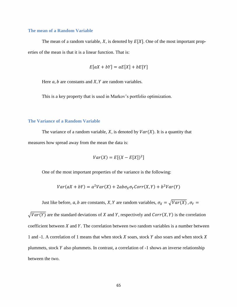
65

The mean of a Random Variable

The mean of a random variable, , is denoted by [ ]. One of the most important prop-

erties of the mean is that it is a linear function. That is:

[ ] [ ] [ ]

Here are constants and are random variables.

This is a key property that is used in Markov’s portfolio optimization.

The Variance of a Random Variable

The variance of a random variable, , is denoted by . It is a quantity that

measures how spread away from the mean the data is:

[ [ ] ]

One of the most important properties of the variance is the following:

Just like before, are constants, are random variables, √

√ are the standard deviations of and , respectively and is the correlation

coefficient between and . The correlation between two random variables is a number between

1 and -1. A correlation of 1 means that when stock soars, stock also soars and when stock

plummets, stock also plummets. In contrast, a correlation of -1 shows an inverse relationship

between the two.

66

As discussed, Markov’s Portfolio Theory manages to find the portfolio with the highest

return and lowest risk. Let be the monthly return on stock random variable and the

nonnegative weight with which stock contributes to the portfolio, respectively and let be the

monthly return on the portfolio. Then, we will have the following relationship between the

monthly returns:

∑

By using the above mentioned properties of the mean and variance, we will have the fol-

lowing relationships:

[ ] ∑ [ ]

∑

∑

( )

Also, the weights will have to add up to 1:

∑

Hence, we have to find the weights that maximize (1) and minimize (2), while keeping

in mind that they also have to satisfy equation (3). Since in equation (2) we have the

( ), the team used Excel to find the correlations between the monthly returns of the

historical prices for all the “Smoothies”70

.

70

For the table, see Appendix page 112

67

The problem of finding the optimal portfolio can be solved using Quadratic program-

ming71

. The team used the MATLAB financial toolbox72

to find the weights that give the optimal

portfolio73

. The values for the weights are presented in the table on the bottom of the page.

We consider that this optimization will give our team an edge because of the lower risk

compared to the one associated with trading only one stock. In business classes offered at WPI,

we learned that even a portfolio for which the stocks were chosen randomly has a significant

lower risk than holding only one stock. This idea is reflected by the figure on the top of the fol-

lowing page.

Symbol Weights

VLO 0.0496

CELG 0.1344

GS 0

XLE 0.0704

AAPL 0

GOOG 0.4966

CVX 0

LVS 0

SLB 0

IWM 0

AMZN 0.1217

BBRY 0

QCOM 0

XOM 0

CAT 0

MDT 0

TOL 0.1273

MS 0

IYR 0

IBM 0 Table 2: Portfolio weights74

71

Ruppert, D. (2011). Statistics and Data Analysis for Financial Engineering. Springer. 72

“Financial Toolbox”.MathWorks.<http://www.mathworks.com/products/finance/description2.html> 73

For the MATLAB code, see Appendix page 112 74

For an overview of the selected stocks, see pages 113 and 114 from the Appendix

68

Figure 5: Naïve (random) diversification

Introduction to the System

The strategy with which our team started off is Mel Raiman’s PTS (Precision Trading

System)75

. Originally, the strategy was designed for manual trading, but the team managed to

transform it into an automated trading system. The advantages of trading the automated version

are obvious; human error is eliminated and the computing speed is far greater and therefore,

judgments such as buying/selling or shorting are made faster. Moreover, the ability to optimize

an automated strategy and the computer’s ability to stick to the programmed rules are also

important advantages. However, with the automation of the strategy, certain aspects of the

original strategy couldn’t be coded because of the complexity of the resulting program. For

example, when a person is told that the difference between the Simple Moving Average line and

the Exponential Moving Average line has to be big enough, they do not need a number to

understand how big this difference has to be. But a computer needs an exact number in order to

75

“Precision Trading System”.PTS.<http://www.precisiontradingsystem.com/AboutTheCourse.html>

69

judge what a “big” or “small” difference is. This would add more input parameters to the code,

which, in turn, would make the code harder to back test over a long period of time.

The team developed multiple strategies, each one with slightly different entry rules, exit

rules and order types. We decided to try different ideas because we realized that each of the

stocks in our portfolio has a different way in which it is traded, a different “personality” as

traders like to call it. In order to trade the six stocks, the team used six different windows in

TradeStation, each one having one of the symbols from our portfolio.

Entry and Exit Rules: The Basic PTS Strategy76

The main PTS strategy used by the team makes use of three different timeframes on the

same symbol: a short timeframe, a medium one and a longer term timeframe.

On the short term timeframe there is a channel made by 3 trend lines. The one in the

center of the channel is a trend line that has as an endpoint the linear regression value of the

closing prices of a pre-specified number of bars and as a start point the delayed linear regression

value of the closing price. The length over which this latter linear regression value is computed

has as input the same pre-specified number as the other linear regression. The exact same idea

was used to make a trend line on each of the other two timeframes. The EasyLanguage code for

making those trend lines can be observed below:

FirstDate_Data1 = date[ Length - 1 ] of Data1;

FirstTime_Data1 = time[ Length - 1 ] of Data1;


76

See Appendix pages 114-121 for the complete strategy

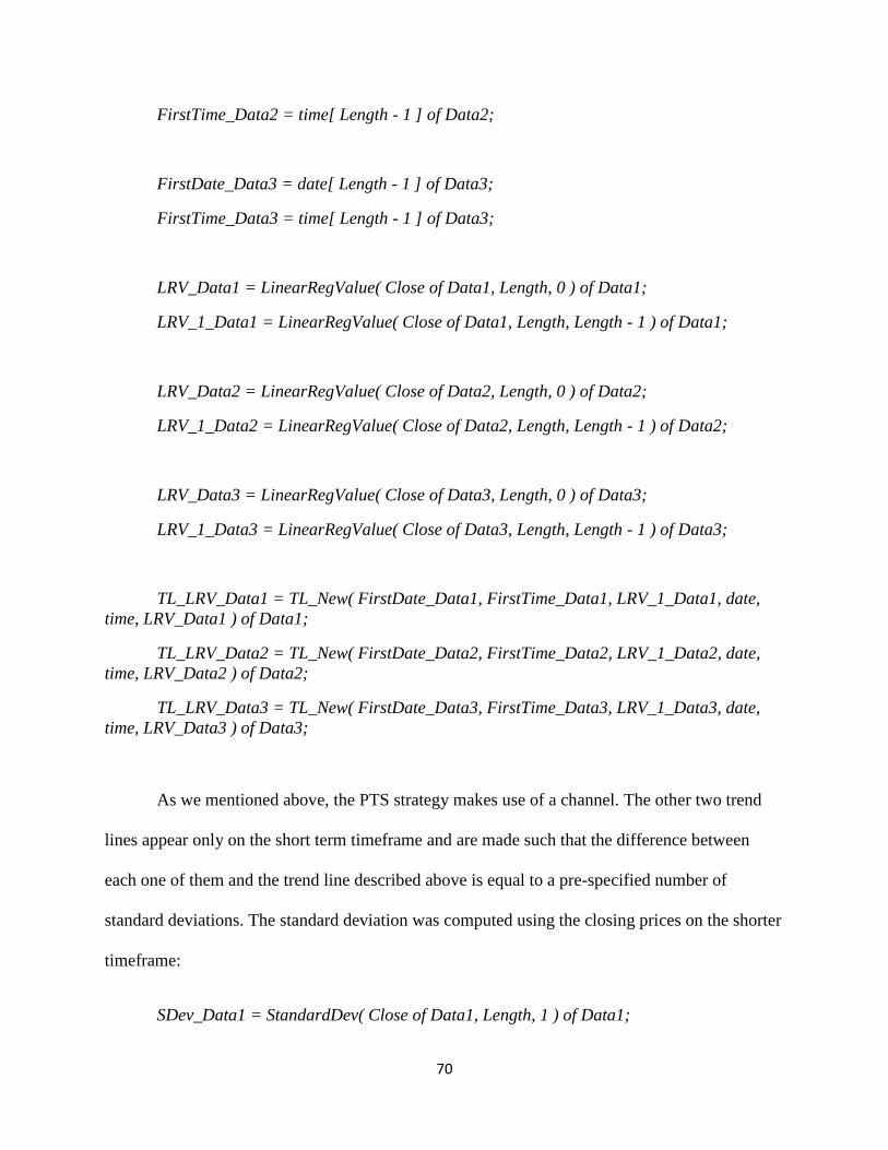
70




LRV_Data1 = LinearRegValue( Close of Data1, Length, 0 ) of Data1;

LRV_1_Data1 = LinearRegValue( Close of Data1, Length, Length - 1 ) of Data1;





TL_LRV_Data1 = TL_New( FirstDate_Data1, FirstTime_Data1, LRV_1_Data1, date,

time, LRV_Data1 ) of Data1;





As we mentioned above, the PTS strategy makes use of a channel. The other two trend

lines appear only on the short term timeframe and are made such that the difference between

each one of them and the trend line described above is equal to a pre-specified number of

standard deviations. The standard deviation was computed using the closing prices on the shorter

timeframe:

SDev_Data1 = StandardDev( Close of Data1, Length, 1 ) of Data1;

71

UpperBand_Data1 = LRV_Data1 + NumDevsUp * SDev_Data1;

LowerBand_Data1 = LRV_Data1 + NumDevsDn * SDev_Data1;

UpperBand_1_Data1 = LRV_1_Data1 + NumDevsUp * SDev_Data1;

LowerBand_1_Data1 = LRV_1_Data1 + NumDevsDn * SDev_Data1;

TL_UB_Data1 = TL_New( FirstDate_Data1, FirstTime_Data1, UpperBand_1_Data1,

date, time, UpperBand_Data1 ) of Data1;

TL_LB_Data1 = TL_New( FirstDate_Data1, FirstTime_Data1, LowerBand_1_Data1,

date, time, LowerBand_Data1 ) of Data1;

The trend lines will envelop the price of the stock. The trader will not be able to clearly

see the price bars because the code generates trend lines on each new bar. The chart will look the

following way:

Figure 9: View of the chart

Those trend lines will generate our buy and sell orders in the following way: if the slope

of the trend lines on the medium and long term timeframes is above a certain threshold it means

72

that the market is in a general uptrend. Therefore, the strategy will look only for longs. In order

to compute the slope of the trend lines, the team used the following code:

TL_Slope_Data2=(LRV_Data2-LRV_1_Data2)/(Length);


Now, the shorter timeframe comes into play. If, on top of the above mentioned

conditions, the close of a bar is above the upper trend line or below the lower trend line in the

channel and we were in a short position, then we have to cover the position. As we know from

statistics, for example, 68% of the data is within one standard deviation from the mean. This

percentage depends on what input the trader decides to use for the number of standard

deviations, but the reasoning behind covering the position is the same. Since the close is outside

the channel, there is something that happened in the market that is abnormal, an outlier.

Moreover, if we weren’t in the market when this happened, then we have to get in and hope for

an uptrend.

Using the same idea, if the slopes of the trend lines on the medium and long term

timeframes are below a certain threshold, then the strategy should only look for shorts. A

symmetrical reasoning was used in this case. The code for those entry rules is the following:

If Close of Data1 > TL_UB_Value_Data1 and TL_Slope_Data2 >= SlopeUp_Data2 and

TL_Slope_Data3 >= SlopeUp_Data3 and marketposition = -1 then

Buy to cover ("Close>UB 1") next bar at market

Else

If Close of Data1 > TL_UB_Value_Data1 and TL_Slope_Data2 >=

SlopeUp_Data2 and TL_Slope_Data3 >= SlopeUp_Data3 and marketposition = 0 then Buy

("Close>UB 2") NrShares shares next bar at market; {TL_LB_Value limit}

73

If Close of Data1 > TL_UB_Value_Data1 and TL_Slope_Data2 <= SlopeDn_Data2 and

TL_Slope_Data3 <= SlopeDn_Data3 and marketposition = 1 then

Sell all contracts next bar at market

Else

If Close of Data1 > TL_UB_Value_Data1 and TL_Slope_Data2 <=

SlopeDn_Data2 and TL_Slope_Data3 <= SlopeDn_Data3 and marketposition=0 then Sell short

NrShares shares next bar at market;

If Close of Data1 < TL_LB_Value_Data1 and TL_Slope_Data2 >= SlopeUp_Data2 and


Buy to cover next bar at market

Else

If Close of Data1 < TL_LB_Value_Data1 and TL_Slope_Data2 >=

SlopeUp_Data2 and TL_Slope_Data3 >= SlopeUp_Data3 and marketposition = 0 then buy


If Close of Data1 < TL_LB_Value_Data1 and TL_Slope_Data2 <= SlopeDn_Data2 and


Sell ("Close<LB 1") all contracts next bar at market

Else

If Close of Data1 < TL_LB_Value_Data1 and TL_Slope_Data2 <=

SlopeDn_Data2 and TL_Slope_Data3 <= SlopeDn_Data3 and marketposition = 0 then sell

short ("Close<LB 2") NrShares shares next bar at market;

As one can see, we have a variable called NrShares that decides how many shares the

strategy should risk at any given time. This NrShares variable was computed using the weights

determined from Markov’s Portfolio Optimization. The team also decided to risk a total of

$350,000 of the $400,000 that the simulated traded account originally has. But this amount of

money changes as the strategy runs. Because we used six windows, each one with one symbol

74

from our portfolio, loaded on three different timeframes, the strategy had to know what the net

profits on each stock are at any given moment in time in order to be able to reinvest the money.

This is why we used All Data Everywhere (ADE) variables77

in the computation of the NrShares

variable.

The way in which ADEs work is that the coder has to make a strategy78

, with which he

loads the information that he needs from each window:

If Getsymbolname="VLO" then

Begin

Value1 = MapSN.Put (InfoMap1, "ProfitSoFar1", Netprofit);

Value1 = ADE.PutBarInfo (Class, "VLO", ADE.BarInterval , ADE.BarID, InfoMap1);

End;

If Getsymbolname="CELG" then

Begin

Value2=MapSN.Put (InfoMap1, "ProfitSoFar2", Netprofit);

Value2=ADE.PutBarInfo (Class, "CELG", ADE.BarInterval, ADE.BarID, InfoMap1);

End;

If Getsymbolname="XLE" then

Begin


Value3=ADE.PutBarInfo (Class, "XLE", ADE.BarInterval , ADE.BarID, InfoMap1);

End;

If Getsymbolname="GOOG" then

77

“All Data Everywhere”.TradeStation Forums. <https://community.tradestation.com/Discussions/Topic.aspx?Topic_ID=33398&SearchTerm=All%20data %20Everywhere&txtExactMatch=> 78

See Appendix pages 121-122

75

Begin


Value4=ADE.PutBarInfo (Class, "GOOG", ADE.BarInterval , ADE.BarID, InfoMap1);

End;

If Getsymbolname="AMZN" then

Begin


Value5=ADE.PutBarInfo (Class, "AMZN", ADE.BarInterval , ADE.BarID, InfoMap1);

End;

If Getsymbolname="TOL" then

Begin


Value6=ADE.PutBarInfo (Class, "TOL", ADE.BarInterval , ADE.BarID, InfoMap1);

End;

Afterwards, each loaded ADEs is used in the PTS strategy and the new account balance and

number of shares is computed:

Value1=ADE.OpenMap (Class, "VLO", ADE.BarInterval);

Value1=ADE.GetBarInfo (Class, "VLO", ADE.BarInterval, ADE.BarID, InfoMap1);

ProfitSoFar1 = MapSN.Get (InfoMap1, "ProfitSoFar1");

Value2=ADE.OpenMap(Class, "CELG", ADE.BarInterval);

Value2=ADE.GetBarInfo (Class, "CELG", ADE.BarInterval, ADE.BarID, InfoMap1);


Value3=ADE.OpenMap(Class, "XLE", ADE.BarInterval);

76

Value3=ADE.GetBarInfo (Class, "XLE", ADE.BarInterval, ADE.BarID, InfoMap1);


Value4=ADE.OpenMap(Class, "GOOG", ADE.BarInterval);

Value4=ADE.GetBarInfo (Class, "GOOG", ADE.BarInterval, ADE.BarID, InfoMap1);


Value5=ADE.OpenMap(Class, "AMZN", ADE.BarInterval);

Value5=ADE.GetBarInfo (Class, "AMZN", ADE.BarInterval, ADE.BarID, InfoMap1);


Value6=ADE.OpenMap(Class, "TOL", ADE.BarInterval);

Value6=ADE.GetBarInfo (Class, "TOL", ADE.BarInterval, ADE.BarID, InfoMap1);


AccBalance=(ProfitSoFar1+ProfitSoFar2+ProfitSoFar3+ProfitSoFar4+ProfitSoFar5+ProfitSo

Far6+StartingBalance)*Weight;

NrShares=floor(AccBalance/close);

Finally, we added a Commentary function not only because we wanted to check that the

ADEs worked, but also because we wanted to see what the typical values for the trend lines’

slopes are:

Commentary( "TL_Slope_Data2=", TL_Slope_Data2, Newline,

"TL_Slope_Data3=", TL_Slope_Data3, Newline,

"Account Balance=", AccBalance, Newline,

"Number of Shares=", NrShares, Newline,

"Profit 1=", ProfitSoFar1,Newline,

"Profit 2=", ProfitSoFar2, Newline,

77




"Profit 6=", ProfitSoFar6, Newline)

As mentioned at the beginning of this chapter, the team created different small variations

of this system in order to try to match the different stocks’ personality. In the following sections,

we will introduce the entry and exit rule variations to the basic PTS, all of them being added on

the shorter term timeframe.

The following two variations both use volume as an extra filter. The main reason in using

volume as an extra filter is to better capture significant movements in the market and, therefore,

to obtain a better winning percentage on the trades. However, as we will see in the next chapter,

the theory doesn’t always work in practice.

PTS with Volume (Version 1)

The first version adds the condition that the volume on the current bar has to be greater

than the volume from 1 bar ago and the volume from one bar ago has to be greater than the

volume from 2 bars ago. Basically, the strategy first looks at an increasing volume in the last 3

bars and, once this condition is verified, it uses the same filters and set-up rules as the basic PTS:

If Volume>=Volume[1] and Volume[1]>=Volume[2] then

78

PTS with Volume (Version 2)

The second version changes a little bit the condition from the first. More specifically, the

new condition is that the volume on the current bar has to be greater than the average of the

volumes from last bar and the one from 2 bars ago:

If Volume>=(Volume[1]+Volume[2])/2 then

PTS with the Relative Strength Indicator (RSI)

The next variation that we developed was by adding the RSI to the conditions that the

PTS basic system has. Whenever we had a long situation in the basic Precision Trading System,

we would check whether or not we had an overbought situation. Hence, if the Relative Strength

Indicator was below an upper bound we would trigger buy signals:

If RSI(Close,LengthRSI)<=UB_RSI then

Begin




Else

If Close of Data1 > TL_UB_Value_Data1 and TL_Slope_Data2 >=

SlopeUp_Data2 and TL_Slope_Data3 >= SlopeUp_Data3 and marketposition = 0 then Buy ("Close>UB

2") NrShares shares next bar at market; {TL_LB_Value limit}

End;

In the same way, whenever we would have a short situation in the basic PTS, we would

check whether or not we had an oversold scenario. Hence, if the RSI was above a lower bound,

we would trigger the sell signals:

79

If RSI(Close,LengthRSI)>=LB_RSI then

Begin




Else

If Close of Data1 > TL_UB_Value_Data1 and TL_Slope_Data2 <=

SlopeDn_Data2 and TL_Slope_Data3 <= SlopeDn_Data3 and marketposition=0 then Sell short


End;

The reason why we used the RSI is the same as the reason why we used volume: to filter

out the wrong signals generated by the basic PTS and, therefore, to increase the number of

profitable trades. However, just like when using the volume, the theory does not match with the

reality.

Mel’s PTS

The last variation of the basic Precision Trading System is a version that is similar to the

one that Mel Raiman used to trade79

. In his system, Mel also used a Simple Moving Average

(SMA) and an Exponential Moving Average (EMA). The idea is that if, on the shorter

timeframe, the SMA and the linear regression cross the EMA with enough separation, we have a

confirmed change of direction in the stocks’ price. The main problem was to convert the phrase

“enough separation” into code. For the long scenario, we decided to impose the condition that

the SMA and the linear regression value of the closing prices for each of the last three bars both

79

Raiman, M. (n.d.). About PTS.

80

have to be greater than the EMA of the closing prices for each of the last three bars, respectively.

More precisely, the EasyLanguage is as follows:

EMA=XAverage(Close, Length) of Data1;

SMA=Average(Close, Length) of Data1;

EMA1=XAverage(Close, Length)[1] of Data1;

SMA1=Average(Close, Length)[1] of Data1;

EMA2=XAverage(Close, Length)[2] of Data1;

SMA2=Average(Close, Length)[2] of Data1;

LRV_Data1_1 = LinearRegValue( Close of Data1, Length, 0 )[1] of Data1;

LRV_Data1_2 = LinearRegValue( Close of Data1, Length, 0 )[2] of Data1;

If (SMA > EMA and LRV_Data1 > EMA) and (SMA1 > EMA1 and LRV_Data1_1 > EMA1) and

(SMA2 > EMA2 and LRV_Data1_2 > EMA2) then

For the short scenarios, the condition is symmetric to the one for longs:

If (SMA < EMA and LRV_Data1 < EMA) and (SMA1 < EMA1 and LRV_Data1_1 < EMA1) and

(SMA2 < EMA2 and LRV_Data1_2 < EMA2) then

PTS and the Variations with Simple Moving Average

The next small change that we decided to make to each one of the above mentioned

variations to the Precision Trading System was to replace the conditions in which the closing of a

bar was used with the SMA of the current bar. More specifically, we replaced the condition

Close of Data1 > TL_UB_Value_Data1 with SMA > TL_UB_Value_Data1 and the condition

Close of Data1 < TL_LB_Value_Data1 with SMA < TL_LB_Value_Data1.

81

Order Types

The next step was to focus on the types of orders that the strategy used. As one can see,

in the basic PTS strategy (and therefore in each one of the variations presented so far) we used

market orders. However, there is a problem with using those kinds of orders with our strategy.

For example, it is possible that the conditions are met to go long, but the next bar falls

completely inside the channel and the price continues falling. Because of these types of

scenarios, the team decided to change each market order to a stop order in the following way:



Buy to cover ("Close>UB 1") next bar at TL_UB_Value_Data1 stop

Now, in the same situation as the one described above, the order will not be filled since a

stop order becomes a market order at the specified price or greater. This should make a

difference in the performance of our strategies. As we will see later in this paper, our intuition is

partially confirmed.

As we promised through the paper, in the next chapter we will present the steps that we

followed to find which of the presented strategies work the best with each individual stock. The

chapter is symbolically called “The Journey to the Best Combination”. Through this journey, we

will also be able to notice which changes to the basic PTS strategy worked, if at all.

82

CHAPTER 5: THE JOURNEY TO THE BEST COMBINATION

In this chapter we will discuss which strategies and timeframes work the best for each

stock. In our “Journey” we made use of the back-testing and of the strategy performance report

functionalities that TradeStation has incorporated. Because of the complexity of the PTS

strategy, of its variations and, even more, because of the timeframes used to trade, the team back-

tested the different variations on half a year’s worth of historical data. We considered that the

market conditions in the past half a year are also a reasonable representation of the future.

However, in the back-testing of the different timeframes, we used 1 year worth of historical data.

We also considered that the most important performance figures from the report are: the

profit factor, the percentage of profitable trades, the percentage of profitable trades on long

positions, the percentage of profitable trades on short positions, the annual return, the return

retracement ratio and the maximum drawdown. The return retracement ratio (RRR) is a measure

similar to the Sharpe ratio. However, the Sharpe ratio can only be computed for back-tests that

cover at least 3 years’ worth of historical data, while the RRR can be computed for any given

length of time.

We decided to back-test the variations on the PTS that do not include the stops at first.

Also, as mentioned in the previous chapter, the PTS strategy makes use of three different

timeframes: a short one, a medium one and a long one. For the following tests, we used a five

minute bar chart for the short timeframe, a 15 minute bar chart for the medium one and a 30

minute bar chart for the longer one.

We will start off by presenting the results from the two systems that make use of volume.

83

Results for the Strategies with Volume

In the following table we can see the different figures for the chosen statistics. The rows

in yellow represent the strategy that we considered to behave better for the particular stock:

Strategy Symbol Weights Profit Factor

Percent of prof Trades

Percent on

longs

Percent on

shorts

Annual Return

RRR/Sharpe Ratio

Max Drawdown

PTS with volume V1

VLO 0.0496 3.28 50% 33.33% 66.67% 60.11% 2.33 4,046.67

CELG 0.1344 0.96 27.78% 44.44% 11.11% -2.55% -0.18 13,429.42

XLE 0.0704 2.75 50% 100% 0% 5.78% 0.58 2,359.92

GOOG 0.4966 1.03 39.47% 50% 27.78% 1.36% 0.09 15,037.01

AMZN 0.1217 1.19 45.45% 56.25% 35.29% 11.09% 1.14 8,969.31

TOL 0.1273 8.28 66.67% 100% 50% 25.41% 1.56 7,046.84

PTS with Volume

V2 VLO 0.0496 2.48 37.50% 25% 50% 48.09% 1.88 4,236.00

CELG 0.1344 1.52 27.78% 44.44% 11.11% 25.58% 1.38 10,331.53

XLE 0.0704 0.99 33.33% 33.33% 33.33% -0.10% -0.01 1,916.15

GOOG 0.4966 0.92 40.00% 54.55% 26.09% -4.27% -0.23 19,860.20

AMZN 0.1217 1.33 43.90% 50.00% 38.10% 18.25% 1.35 10,219.97

TOL 0.1273 0.56 16.67% 50.00% 0% -17.63% -0.99 13,323.37

Table 3: Performance for PTS with volume

For VLO and TOL we chose the first version of the PTS with volume since it

outperformed the second version in all the statistics. Next, we think that the first version is also

better suited for XLE and GOOG, since each one has higher RRRs and profit factors than the

second version of the PTS strategy with volume. It is true that for XLE the first version of the

strategy seemed to miss a short opportunity, but since the Energy Select Sector is not a volatile

stock (the standard deviation of the historical monthly return is 0.06, below the average of our

top 20 “smoothies”) we think that this strategy will be able to capture the big trends better. The

winning percentages on trades for CELG are exactly the same, but the second version has a

significantly higher profit factor, a lower drawdown and a higher return retracement ratio. When

it comes to AMZN, we decided to go for the second version because of the higher winning

84

percentage on shorts and because of the higher RRR. Albeit the winning percentage on long

positions is lower, Amazon is a more volatile stock (the standard deviation of the historical

monthly return is 0.19, above the average of our top 20 “smoothies”) and having a strategy that

can perform well on uptrends and downtrends is important.

Results for all the Strategy Variations

In the following table, one can observe the results for each strategy on each of the 6

symbols. Notice that for the strategy with volume, we added the best combination that was

determined in the previous section. Also, one might notice that the table is organized with

respect to the strategies traded and not to the symbols. This is because we wanted to compute

some of the statistics for our portfolio in the eventuality that we would have traded the same

exact strategy on each stock. The results surprised us mostly because of the big difference in

performance between some of the small variations that we made to the original PTS:

Strategy Symbol Weights Profit Factor


Percent on longs

Percent on

shorts

Annual Return

RRR/Sharpe Ratio

Max Drawdown

PTS

basic VLO 0.0496 2.95 50.00% 25% 75.00% 53.49% 2.06 4,752.29

CELG 0.1344 1.89 30.00% 50% 10.00% 37.16% 1.7 8,915.68

XLE 0.0704 1.27 50.00% 66.67% 33.33% 3.27% 0.26 1,875.64

GOOG 0.4966 0.79 36.17% 50% 21.74%

-11.61%

-0.62 24,196.59

AMZN 0.1217 1.39 42.22% 41.67% 42.86% 23.93% 2.30 8,501.71

TOL 0.1273 0.34 14.29% 33.33% 0.00%

-40.03%

-1.43 18,679.02

Portfolio 1 1.094503 37.11% 44.45% 30.49% -0.07%

66,920.93

PTS with

volume VLO (Volume V1) 0.0496 3.28 50% 33.33% 66.67% 60.11% 2.33 4,046.67

CELG (Volume V2) 0.1344 1.52 27.78% 44.44% 11.11% 25.58% 1.38 10,331.53

85

XLE (Volume V1) 0.0704 2.75 50% 100% 0% 5.78% 0.58 2,359.92

GOOG (Volume V1) 0.4966 1.03 39.47% 50% 27.78% 1.36% 0.09 15,037.01

AMZN (Volume V2) 0.1217 1.33 43.90% 50.00% 38.10% 18.25% 1.35 10,219.97

TOL (Volume V1) 0.1273 8.28 66.67% 100% 50% 25.41% 1.56 7,046.84

Portfolio 1 2.287979 46.30% 62.96% 32.28% 12.96%

49041.94

PTS

with RSI VLO 0.0496 3.06 50.00% 25% 75.00% 54.65% 2.1 4622.35

CELG 0.1344 2 30.00% 50% 10.00% 39.34% 1.76 8,785.34

XLE 0.0704 1.29 50.00% 66.67% 33.33% 3.46% 0.28 1,875.64

GOOG 0.4966 0.8 36.17% 50% 21.74%

-11.01%

-0.6 23,643.03

AMZN 0.1217 1.46 44.44% 45.83% 42.86% 26.75% 2.83 8,096.21

TOL 0.1273 0.34 14.29% 33.33% 0.00%

-39.97%

-1.43 18,665.19

Portfolio 1 1.129636 37.48% 45.14% 30.49% 0.94%

65687.76

Mel's PTS

VLO 0.0496 2.18 50.00% 25% 75.00% 44.62% 1.79 5,705.10

CELG 0.1344 1.51 22.22% 37.50% 10.00% 24.09% 1.82 8,224.63

XLE 0.0704 0.86 50.00% 66.67% 33.33% -2.44% -0.22 2,217.69

GOOG 0.4966 0.89 42.42% 62.50% 23.53% 5.23% -0.38 21,662.30

AMZN 0.1217 1.46 46.88% 55.56% 35.17% 23.29% 1.16 7,430.06

TOL 0.1273 0.3 14.29% 33.33% 0.00%

-47.57%

-1.5 20,795.35

Portfolio 1 1.029462 37.64% 46.76% 29.51% 4.66%

66,035.13

PTS with SMA

PTS

basic VLO 0.0496 1.93 40.00% 20% 60.00% 41.27% 1.72 6,078.90

CELG 0.1344 2.37 38.89% 66.67% 11.11% 43.74% 1.9 8,142.90

XLE 0.0704 0.95 50.00% 66.67% 33.33% -0.82% -0.07 1,898.45

GOOG 0.4966 0.88 38.64% 57.14% 21.74% -6.05% -0.36 20,180.58

AMZN 0.1217 1.57 47.73% 50.00% 45.45% 29.23% 3.49 6,125.32

TOL 0.1273 0.32 14.29% 33.33% 0.00%

-42.04%

-1.47 18,996.19

Portfolio 1 1.149949 38.26% 48.97% 28.61% 3.07%

61,422.34

PTS with

volume VLO (Volume V1) 0.0496 1.66 44.44% 25% 60.00% 34.60% 1.52 6,696.79

CELG (Volume V2) 0.1344 2.12 27.78% 44.44% 11.11% 38.19% 1.79 7,652.32

XLE (Volume V1) 0.0704 3.97 66.67% 100.00% 50.00% 9.09% 0.93 1,951.32

86

GOOG (Volume V1) 0.4966 0.88 38.46% 66.67% 14.29% -5.41% -0.39 18,168.84

AMZN (Volume V2) 0.1217 1.43 46.51% 50.00% 42.86% 23.70% 3.40 6,758.46

TOL (Volume V1) 0.1273 0.5 25% 50% 0%

-21.42%

-1.16 15,088.87

Portfolio 1 1.321441 41.48% 56.02% 29.71% 4.96%

56316.6

PTS

with RSI VLO 0.0496 1.75 40.00% 20% 60.00% 36.10% 1.59 6605.06

CELG 0.1344 2.21 33.33% 55.56% 11.11% 40.35% 1.81 8,194.90

XLE 0.0704 1.09 50.00% 66.67% 33.33% 1.25% 0.10 1,872.65

GOOG 0.4966 0.94 40.91% 61.90% 21.74% -2.68% -0.16 19.051.69

AMZN 0.1217 1.57 47.73% 50.00% 45.45% 29.58% 3.48 6,209.23

TOL 0.1273 0.29 14.29% 33.33% 0.00%

-48.78%

-1.68 20,960.51

Portfolio 1 1.15535 37.71% 47.91% 28.61% 3.36%

43842.35

Mel's PTS

VLO 0.0496 2.71 50.00% 25% 75.00% 52.27% 2.06 4,895.53

CELG 0.1344 1.29 25.00% 33.33% 14.29% 14.07% 0.81 9,454.31

XLE 0.0704 1.09 50.00% 66.67% 33.33% 1.24% 0.10 1,864.72

GOOG 0.4966 1.39 50.00% 75.00% 25.00% 9.64% 0.70 14,378.41

AMZN 0.1217 0.62 36.00% 38.46% 33.33%

-22.14%

-1.17 9,884.05

TOL 0.1273 0.46 20.00% 50.00% 0.00%

-25.10%

-1.24 14,756.01

Portfolio 1 1.208814 38.50% 48.08% 30.16% 3.47%

55,233.03

Table 4: Performance for the 8 variations on PTS

This difference can be more easily noted when we organize the above table after each

symbol associated with each of the eight strategy variations. The following table does exactly

this and also sorts the information with respect to the profit factor. We chose to use the profit

factor because most of the other performance statistics have a positive relationship with it. The

rows highlighted in yellow represent what we believed to be the best choices of strategies for

each stock:

87

Symbol (Strategy) Weights Profit Factor


Percent on longs

Percent on

shorts

Annual Return

RRR/Sharpe Ratio

Max Drawdown

TOL (Volume V1) 0.1273 8.28 66.67% 100% 50% 25.41% 1.56 7,046.84

XLE (Volume V1&SMA) 0.0704 3.97 66.67% 100.00% 50.00% 9.09% 0.93 1,951.32

VLO (Volume V1) 0.0496 3.28 50% 33.33% 66.67% 60.11% 2.33 4,046.67

VLO (RSI) 0.0496 3.06 50.00% 25% 75.00% 54.65% 2.1 4622.35

VLO (PTS basic) 0.0496 2.95 50.00% 25% 75.00% 53.49% 2.06 4,752.29

XLE (Volume V1) 0.0704 2.75 50% 100% 0% 5.78% 0.58 2,359.92

VLO (Mel's PTS&SMA) 0.0496 2.71 50.00% 25% 75.00% 52.27% 2.06 4,895.53

CELG (PTS basic&SMA) 0.1344 2.37 38.89% 66.67% 11.11% 43.74% 1.9 8,142.90

CELG (RSI&SMA) 0.1344 2.21 33.33% 55.56% 11.11% 40.35% 1.81 8,194.90

VLO (Mel's PTS) 0.0496 2.18 50.00% 25% 75.00% 44.62% 1.79 5,705.10

CELG (Volume V2&SMA)

0.1344 2.12 27.78% 44.44% 11.11% 38.19% 1.79 7,652.32

CELG (RSI) 0.1344 2 30.00% 50% 10.00% 39.34% 1.76 8,785.34

VLO (PTS basic&SMA) 0.0496 1.93 40.00% 20% 60.00% 41.27% 1.72 6,078.90

CELG (PTS basic) 0.1344 1.89 30.00% 50% 10.00% 37.16% 1.7 8,915.68

VLO (RSI&SMA) 0.0496 1.75 40.00% 20% 60.00% 36.10% 1.59 6605.06

VLO (Volume V1&SMA) 0.0496 1.66 44.44% 25% 60.00% 34.60% 1.52 6,696.79

AMZN (PTS basic&SMA)

0.1217 1.57 47.73% 50.00% 45.45% 29.23% 3.49 6,125.32

AMZN (RSI&SMA) 0.1217 1.57 47.73% 50.00% 45.45% 29.58% 3.48 6,209.23

CELG (Volume V2) 0.1344 1.52 27.78% 44.44% 11.11% 25.58% 1.38 10,331.53

CELG (Mel's PTS) 0.1344 1.51 22.22% 37.50% 10.00% 24.09% 1.82 8,224.63

AMZN (RSI) 0.1217 1.46 44.44% 45.83% 42.86% 26.75% 2.83 8,096.21

AMZN (Mel's PTS) 0.1217 1.46 46.88% 55.56% 35.17% 23.29% 1.16 7,430.06

AMZN (Volume V2&SMA)

0.1217 1.43 46.51% 50.00% 42.86% 23.70% 3.40 6,758.46

AMZN (PTS basic) 0.1217 1.39 42.22% 41.67% 42.86% 23.93% 2.30 8,501.71

GOOG (Mel's PTS&SMA)

0.4966 1.39 50.00% 75.00% 25.00% 9.64% 0.70 14,378.41

AMZN (Volume V2) 0.1217 1.33 43.90% 50.00% 38.10% 18.25% 1.35 10,219.97

XLE (RSI) 0.0704 1.29 50.00% 66.67% 33.33% 3.46% 0.28 1,875.64

CELG (Mel's PTS&SMA) 0.1344 1.29 25.00% 33.33% 14.29% 14.07% 0.81 9,454.31

XLE (PTS basic) 0.0704 1.27 50.00% 66.67% 33.33% 3.27% 0.26 1,875.64

XLE (RSI&SMA) 0.0704 1.09 50.00% 66.67% 33.33% 1.25% 0.10 1,872.65

XLE (Mel's PTS&SMA) 0.0704 1.09 50.00% 66.67% 33.33% 1.24% 0.10 1,864.72

GOOG (Volume V1) 0.4966 1.03 39.47% 50% 27.78% 1.36% 0.09 15,037.01

XLE (PTS basic&SMA) 0.0704 0.95 50.00% 66.67% 33.33% -0.82% -0.07 1,898.45

GOOG (RSI&SMA) 0.4966 0.94 40.91% 61.90% 21.74% -2.68% -0.16 19.051.69

GOOG (Mel's PTS) 0.4966 0.89 42.42% 62.50% 23.53% 5.23% -0.38 21,662.30

GOOG (PTS basic&SMA)

0.4966 0.88 38.64% 57.14% 21.74% -6.05% -0.36 20,180.58

88

GOOG (Volume V1&SMA)

0.4966 0.88 38.46% 66.67% 14.29% -5.41% -0.39 18,168.84

XLE (Mel's PTS) 0.0704 0.86 50.00% 66.67% 33.33% -2.44% -0.22 2,217.69

GOOG (RSI) 0.4966 0.8 36.17% 50% 21.74% -11.01% -0.6 23,643.03

GOOG (PTS basic) 0.4966 0.79 36.17% 50% 21.74% -11.61% -0.62 24,196.59

AMZN (Mel's PTS&SMA)

0.1217 0.62 36.00% 38.46% 33.33% -22.14% -1.17 9,884.05

TOL (Volume V1&SMA) 0.1273 0.5 25% 50% 0% -21.42% -1.16 15,088.87

TOL (Mel's PTS&SMA) 0.1273 0.46 20.00% 50.00% 0.00% -25.10% -1.24 14,756.01

TOL (PTS basic) 0.1273 0.34 14.29% 33.33% 0.00% -40.03% -1.43 18,679.02

TOL (RSI) 0.1273 0.34 14.29% 33.33% 0.00% -39.97% -1.43 18,665.19

TOL (PTS basic&SMA) 0.1273 0.32 14.29% 33.33% 0.00% -42.04% -1.47 18,996.19

TOL (Mel's PTS) 0.1273 0.3 14.29% 33.33% 0.00% -47.57% -1.5 20,795.35

TOL (RSI&SMA) 0.1273 0.29 14.29% 33.33% 0.00% -48.78% -1.68 20,960.51 Table 5: Sorted performance for the 8 variations on PTS

All of the choices made were obvious, except the one for AMZN. There are two

strategies that had very similar performance when applied to this symbol: the one highlighted in

yellow and the one that is directly below it. We decided to use the basic PTS with the simple

moving average added to it because the complexity of this program is smaller than the one

associated with also having a relative strength indicator besides the two conditions that were

mentioned. Moreover, the performance statistics show us that adding the RSI does not

significantly improve the strategy.

As we noticed, some of the additional technical indicators did not give an extra advantage

to the system. But there are some changes that improved the system in a very surprising way. For

example, we can see that for TOL, seven of the strategies ranked the worst of all, while one of

them (the PTS with the first version of the volume condition) ranked on top.

With the best combination of strategies found, we can figure out what the performance

statistics for our portfolio would be:

89

Symbol (Strategy) Weights Profit Factor


Percent on longs

Percent on

shorts

Annual Return

RRR/Sharpe Ratio

Max Drawdown

VLO (Volume V1) 0.0496 3.28 50% 33.33% 66.67% 60.11% 2.33 4,046.67

CELG (PTS basic&SMA) 0.1344 2.37 38.89% 66.67% 11.11% 43.74% 1.9 8,142.90

XLE (Volume V1&SMA) 0.0704 3.97 66.67% 100.00% 50.00% 9.09% 0.93 1,951.32

GOOG (Mel's PTS&SMA)

0.4966 1.39 50.00% 75.00% 25.00% 9.64% 0.70 14,378.41

AMZN (PTS basic&SMA)

0.1217 1.57 47.73% 50.00% 45.45% 29.23% 3.49 6,125.32

TOL (Volume V1) 0.1273 8.28 66.67% 100% 50% 25.41% 1.56 7,046.84

Portfolio 1 2.696091 53.33% 70.83% 41.37% 21.08%

41,691.46 Table 6: Performance for our best combination

Now that we have an idea of which strategies work best with the personality of each one

of the stocks from our portfolio, we are ready to test different timeframe combinations for our

strategy.

Timeframe Analysis

As we saw in the previous section, the smallest change in the strategy’s code can

sometimes create a big difference in performance and sometimes it can make no important

difference. Having this in mind, our team decided to test for the three different combinations of

timeframes that PTS uses: the short term one, the medium term one and the long term one. For

this analysis we used one year of historical data. The following table presents the performance

figures for three different timeframe triples:

90

Timeframes Symbol Weights Profit Factor


Percent on

longs

Percent on

shorts

Annual Return

RRR/Sharpe Ratio

Max Drawdown

5vs15vs30

VLO 0.0496 3.26 50.00% 50% 50.00% 41.48% 1.84 4150.73

CELG 0.1344 0.99 35.71% 57.14% 14.29% -0.92% -0.04 19,167.06

XLE 0.0704 1.97 60% 57.14% 62.50% 10.27% 1.09 3,293.46

GOOG 0.4966 1.41 45.24% 55.00% 36.36% 13.22% 0.86 19,530.96

AMZN 0.1217 1.27 43.53% 47.62% 39.53% 15.50% 0.88 7,182.02

TOL 0.1273 4.62 50% 75% 25% 29.57% 1.57 8,332.80

Portfolio 1 1.876331 47.41% 56.98% 37.95% 14.87% 0.896657 61,657.03

10vs30vs60

VLO 0.0496 2.48 25.00% 40.00% 14.29% 47.57% 2.11 5969.04

CELG 0.1344 0.55 34.29% 58.82% 11.11% -30.59% -3.15 20,302.66

XLE 0.0704 0.35 20.00% 30.00% 10.00% -23.02% -3.17 8,168.13

GOOG 0.4966 0.63 31.25% 43.75% 18.75% -17.39% -2.79 54,190.57

AMZN 0.1217 0.67 35.19% 38.46% 32.14% -18.17% -3.83 11,464.88

TOL 0.1273 0.53 50% 60% 40% -11.40% -1.85 13,122.25

Portfolio 1 0.683434 32.62% 45.17% 21.05% -15.67% -2.629 113,217.53

2vs5vs15

VLO 0.0496 n/a 100.00% 100% 0.00% 47.59% 1.82 4146.44

CELG 0.1344 1.2 41.03% 57.89% 25.00% 10.89% 0.51 20,171.05

XLE 0.0704 1.15 44.44% 60.00% 25.00% 2.04% 0.18 3,818.08

GOOG 0.4966 0.95 34.12% 48.78% 20.45% -3.17% -0.43 39,367.32

AMZN 0.1217 0.94 33.09% 37.68% 28.36% -5.80% -0.44 12,360.57

TOL 0.1273 2.47 50% 100% 0% 12.96% 1.58 15,078.12

Portfolio 1 #VALUE! 50.45% 67.39% 16.47% 3.34% 0.105536 94,941.58

Table 7: Timeframe analysis

Just like before, we also computed different performance statistics for our portfolio. It is

important to notice that the figures for the RRR are just an approximation of the real return

retracement ratio. The way it was computed in this table is by using the RRR of each individual

stock and multiplying it by the corresponding weight. Afterwards, all the resulting numbers were

added together. After studying the Sharpe ratio and some properties for the variance of a random

variable, we know that the actual RRR also depends on the correlation between each stock.

Hence, albeit the figures for the portfolio’s RRR are not accurate, they offer some insight on the

91

overall return to risk ratio for our portfolio. The team decided that the 5 minute bar short

timeframe, 15 minute bar medium timeframe and the 30 minute bar long timeframe are the best

combination for our portfolio since it has a better winning percentage on short positions and it

has the highest return retracement ratio. Also, the maximum drawdown is significantly smaller

than that for the other two combinations of timeframes.

Now that we have tested for different timeframes, we can move on to the next step in our

“journey”.

Analysis for Different Types of Orders

As we mentioned in chapter 4, our team also made use of stop orders. In this section we

will see if the addition of stop orders makes a difference in the performance of our strategy. The

following table presents results of the back testing on two years’ worth of historical data for each

individual stock with market orders and with stop orders:

Symbol Weights Net Profit

Profit Factor


Percent on

longs

Percent on

shorts

Annual Return

RRR/Sharpe Ratio

Max Drawdown

Without Stop

VLO 0.0496 14533.08 3.87 64.29% 57.14% 71.43% 30.39% 0.60 8712.08

CELG 0.1344 -585.23 0.99 38.57% 60.00% 17.14% -0.62% -0.02 19,237.50

XLE 0.0704 10304.93 1.86 50% 42.86% 56.52% 17.46% 0.58 4,772.63

GOOG 0.4966 66828.40 1.36 42.86% 44.44% 41.30% 16.26% 0.47 32,284.77

AMZN 0.1217 33968.14 1.43 40.34% 40.23% 40.45% 29.30% 0.64 11,585.56

TOL 0.1273 20129.78 2.96 50% 66.67% 33.33% 18.63% 0.81 14,380.03

Portfolio 1 145179.10 1.682167 47.68% 51.89% 43.36% 16.67% 0.482307 90,972.57

With Stop

VLO 0.0496 16139.29 8.47 77.78% 75% 80.00% 32.84% 0.65 8764.94

CELG 0.1344 -8265.95 0.85 38.24% 58.82% 17.65% -8.09% -0.23 26,060.78

92

XLE 0.0704 7585.75 1.52 47.62% 42.86% 52.38% 13.41% 0.46 5,523.65

GOOG 0.4966 100190.62 1.53 44.32% 46.67% 41.86% 22.74% 0.67 33,997.09

AMZN 0.1217 34431.29 1.46 42.14% 41.77% 42.50% 29.60% 0.58 11,544.59

TOL 0.1273 20057.51 7.39 83.33% 75% 100% 18.57% 0.93 17,099.94

Portfolio 1 170138.51 2.519587 55.57% 56.69% 55.73% 18.74% 0.555409 102,990.99

Table 8: Order type analysis

Just like before, the rows highlighted in yellow represent the choices that we made for

each individual stock. The hardest decision was for Amazon. Albeit the figures are similar, we

decided to opt for using a stop order since the winning percentages on both long trades and short

trades are a little bit bigger. In the following table, we put together our above mentioned choices

and computed the performance figures for our portfolio:

Symbol Strategy Weights Net Profit Profit Factor


Percent on

longs

Percent on

shorts

Annual Return

RRR/ Sharpe Ratio

Max Drawdown

VLO PTS Volume

V1&Stop 0.0496 16139.29 8.47 77.78% 75% 80.00% 32.84% 0.65 8764.94

CELG PTS basic&SMA 0.1344 -585.23 0.99 38.57% 60.00% 17.14% -0.62% -0.02 19,237.50

XLE PTS Volume

V1&SMA 0.0704 10304.93 1.86 50% 42.86% 56.52% 17.46% 0.58 4,772.63

GOOG Mel’s

PTS&SMA&Stop 0.4966 100190.6 1.53 44.32% 46.67% 41.86% 22.74% 0.67 33,997.09

AMZN PTS

basic&SMA&Stop 0.1217 34431.29 1.46 42.14% 41.77% 42.50% 29.60% 0.58 11,544.59

TOL PTS Volume

V1&Stop 0.1273 20057.51 7.39 83.33% 75% 100% 18.57% 0.93 17,099.94

Portfolio

1 180538.41 2.562339 56.02% 56.88% 56.34% 20.03% 0.592081 95,416.69 Table 9: Final combination of strategies

This combination of strategies gives us an edge over the previously mentioned one.

Evidently, all the performance statistics were improved, except the maximum drawdown, which

became slightly bigger. The team was also satisfied with the fact that we managed to obtain

similar winning percentages on long positions and short positions giving us more confidence that

this strategy is also more robust across different market conditions.

93

This brings us to the last step in our “journey”.

The Addition of Slippage and Commission

The team used $7 for Commission80

and $1 for Slippage. The results of the back testing81

on two years’ worth of data with the mentioned commission and slippage are presented in the

following table:

Symbol Strategy Weights Net Profit Profit Factor


Percent on

longs

Percent shorts

Annual Return

RRR/ Sharpe Ratio

Max Drawdown

VLO PTS Volume

V1&Stop 0.0496 15980.64 8.29 77.78% 75% 80.00% 32.65% 0.85 8780.94

CELG PTS basic&SMA 0.1344 -1026.60 0.98 39.13% 60.00% 17.65% -1.08% -0.06 19,504.24

XLE PTS Volume

V1&SMA 0.0704 9605.20 1.78 50% 42.86% 56.52% 16.47% 0.63 4,868.63

GOOG Mel's

PTS&SMA&Stop 0.4966 99759.74 1.52 44.32% 46.67% 41.86% 22.69% 0.79 34,150.10

AMZN PTS

basic&SMA&Stop 0.1217 32451.79 1.43 42.14% 41.77% 42.50% 28.33% 0.74 11,988.01

TOL PTS Volume

V1&Stop 0.1273 20165.52 7.38 83.33% 75% 100% 18.68% 0.96 17,288.70

Portfolio

1 176936.29 2.536545 56.12% 56.88% 56.42% 19.73% 0.683028 96,580.62 Table 10: Performance with slippage and commission

It is important to notice that, all the presented performance figures are before optimizing

the inputs of our strategy. This brings us to the next chapter.

80

“Competitive Pricing”. TradeStation. <https://www.tradestation.com/pricing> 81

See Appendix page 123-128 for the complete strategy performance report

94

CHAPTER 6: TESTING THE QUALITY AND ROBUSTNESS OF OUR STRATEGY

In this chapter we will optimize some of the inputs of our system and, afterwards, we will

attempt to give other measurements for our strategy’s performance.

Optimization and Walk-Forward Analysis

Before starting the actual optimization analysis, one has to understand the disadvantages

of this method. Yes, if one is not careful when optimizing, there are some disadvantages to this

kind of analysis. In order to understand them, we will have to make a small incursion into the

world of Financial Mathematics.

Ito’s Lemma

Although it was not discovered by Ito, the Japanese’s developed theory for rocket science

was applied to the field of Financial Mathematics, resulting in one of the most important results:

The first term in the sum on the right hand side of the equation is the one that models the

general direction and growth of a stock’s price, while the second term in the sum is the one that

models the randomness of a stock’s price.

95

Now, by knowing this, we realize even more that each stock has a signal or pattern part

and a random part or noise, as Dennis Meyers likes to refer to them in his paper82

. When

optimizing, we want our strategy to better catch the pattern part of a signal and not the random

part. This is because the pattern, as the name implies, will repeat in the future, while the noise

will not. Hence, when the strategy is optimized on in-sample data and ran afterwards on out-of-

sample data, we will be looking for the combination of inputs that gives the best performance on

the latter data, since this shows that the parameters were fitted to the pattern part of the stock’s

price and not to the noise.

Now, our basic PTS strategy has seven inputs that could be optimized: the length of the

linear regression, the number of standard deviations for the upper trend line, the number of

standard deviations for the lower trend line, the slope for the medium timeframe and for the long

timeframe above which we would only look for longs and the slope for the same timeframes

below which we would only look for shorts. Since the length of the linear regression is set to 23,

a number that is commonly used among traders because it represents the average number of

trading days in a month and since the number of standard deviations were selected such that 68%

of the closing prices would fall within the channel, the slopes remain the only parameters that we

would have to optimize for.

Because of the complexity of the program, we were only able to optimize the strategy

using three months’ worth of historical data. Moreover, since the input parameter that was used

so far for the upward trending slopes was 0.05 and the one for the downward trending slopes was

-0.05, our team decided to optimize for parameters that range from 0.01 to 0.09 and from -0.09 to

82

Meyers, D. (2004). Curve Fitting, Data Mining, Strategy Optimization & Walk Forward Analysis Using the Acceleration System.

96

-0.01, respectively, with an increment equal to 0.01. This resulted in a number of 6561 different

combinations of those 4 parameters. In order to reduce the computing time, we used the genetic

algorithm with the population size equal to 50 and with the number of individuals equal to 30.

Again, we were limited to those numbers because of the complexity of our strategy. Because of

the small number of tests and because of the small number of trades that our strategy generates83

,

our team decided to see those results in a skeptical way. Moreover, we agreed that, once we

would obtain an optimized set of parameters, we would back test it again on one year’s worth of

historical out-of-sample data and compare it to our initial choice back-tested over the same

period of time.

In the next section, we will present the results of our analysis and the comparisons made

for each of the 6 stocks in our portfolio.

Optimized Parameters vs. the Initial “Guess”

Before we delve into the comparison between the one year out-of-sample results for our

strategy with the optimized parameters and the results for the strategy with our initial guess, we

will first present the statistics for our optimization over a three month period.

Symbol Weights Parameters Profit Factor

Number of

Trades


Percent on

longs

Percent shorts

Annual Return

RRR/ Sharpe Ratio

Max Drawdown

VLO 0.0496 0.03,-0.01,0.06,-

0.09 0.96 6 50.00% 33.33% 66.67% -1.48% -0.17 2470.52

CELG 0.1344 0.01,-0.02,0.01,-

0.03 5.86 19 47.37% 60.00% 33.33% 102.29% 4.23 3,361.45

XLE 0.0704 0.02,-0.01,0.02,-

0.03 1.31 15 46.67% 50.00% 42.86% 12.81% 0.70 1,524.63

GOOG 0.4966 0.08,-0.06,0.01,-

0.05 2.26 10 50.00% 60.00% 40.00% 39.04% 2.81 12,779.41

83

See Appendix page 123-128 for the complete strategy performance report

97

AMZN 0.1217 0.02,-0.02,0.09,-

0.02 4.31 13 69.23% 83.33% 57.14% 71.68% 3.32 3,712.45

TOL 0.1273 0.02,-0.05,0.06,-

0.02 n/a 0 0% 0.00% 0% 0.00% 0.00 8,614.65

Portfolio 1

n/a 63 43.88% 47.78% 40.00% 42.69% 2.40885 32,463.11 Table 11: Optimization over 3 months’ worth of data

As we can see in the table, our concern that the strategy will generate a small number of

trades was well founded. Nevertheless, as we mentioned before, the next step was to use the

parameters that TradeStation thought to be optimal for the past three months and test them over

an out-of-sample one-year-long time period. The results are presented in the following table:



Percent on longs

Percent shorts

Annual Return

RRR/Sharpe Ratio

Max Drawdown

VLO 0.0496 0.03,-0.01,0.06,

-0.09 n/a 100.00% 100.00% 0.00% 11.52% 0.29 5702.76

CELG 0.1344 0.01,-0.02,0.01,

-0.03 0.78 33.33% 35.90% 30.77% -17.05% -2.08 17,267.00

XLE 0.0704 0.02,-0.01,0.02,-

0.03 0.91 34.55% 32.14% 37.04% -3.84% -0.63 4,565.99

GOOG 0.4966 0.08,-0.06,0.01,-

0.05 1.45 45.24% 47.62% 42.86% 14.53% 1.07 21,247.28

AMZN 0.1217 0.02,-0.02,0.09,-

0.02 1.08 35.71% 40.48% 30.95% 6.84% 0.41 12,578.41

TOL 0.1273 0.02,-0.05,0.06,-

0.02 5.53 66.67% 100.00% 33.33% 35.44% 1.33 7,702.15

Portfolio 1

52.58% 59.36% 29.16% 10.57% 0.441048 69,063.59 Table 12: Results for optimized parameters over 1 year worth of data

From the above table and from the discussion that we had about Ito’s lemma, we realize

that the optimizations made over the three months for CELG and XLE mostly caught the noise or

the randomness. Since this is not what we want, we can rule out from the very beginning those

two optimizations. However, we can’t arrive at the same conclusion when it comes to the other

four stocks. In order to have a benchmark, we will present in the following table the performance

results for testing our strategy with the initial parameters over the same time period:

98



Percent on longs

Percent shorts

Annual Return

RRR/Sharpe Ratio

Max Drawdown

VLO 0.0496 0.05,-0.05,0.05,-

0.05 n/a 100.00% 100.00% 0.00% 25.86% 0.74 3851.70

CELG 0.1344 0.05,-0.05,0.05,-

0.05 0.93 36.36% 56.25% 17.65% -3.56% -0.26 19,640.37

XLE 0.0704 0.05,-0.05,0.05,-

0.05 1.06 56.25% 42.86% 66.67% 1.23% 0.11 4,056.46

GOOG 0.4966 0.05,-0.05,0.05,-

0.05 1.35 45.24% 47.62% 42.86% 12.02% 0.99 22.239.21

AMZN 0.1217 0.05,-0.05,0.05,-

0.05 1.68 47.30% 48.65% 45.95% 34.77% 1.66 6,854.26

TOL 0.1273 0.05,-0.05,0.05,-

0.05 2.45 50.00% 50.00% 0.00% 8.39% 0.65 14,688.96

Portfolio 1

55.86% 57.56% 28.86% 12.16% 0.785905 49,091.75 Table 13: Results for initial guess over 1 year worth of data

Our initial guess worked better for most of the stocks in our portfolio. For GOOG, the

differences were very small, while the differences for TOL were too big to be unnoticed. The

optimized parameters seemed to have caught the trend in this stock’s price better than our initial

“guess” did.

We decided to further test the optimized strategies for those two stocks over a two-year-

long timeframe. The following table presents the performance figures just for the two stocks:



Percent on longs

Percent shorts

Annual Return

RRR/Sharpe Ratio

Max Drawdown

GOOG 0.4966 0.08,-0.06,0.01,-

0.05 1.4 43.33% 45.65% 40.91% 18.48% 0.77 34,150.10

TOL 0.1273 0.02,-0.05,0.06,-

0.02 2.03 66.67% 100.00% 42.86% 20.44% 0.67 24,903.51

GOOG 0.4966 0.05,-0.05,0.05,-

0.05 1.52 44.32% 46.67% 41.86% 22.69% 0.79 34,150.10

TOL 0.1273 0.05,-0.05,0.05,-

0.05 7.38 83.33% 75% 100% 18.68% 0.96 17,288.70

Table 14: Optimization vs. initial guess

99

Since the performance figures for our initial guess offered better results than the ones

obtained by optimizing the four input parameters for our strategy over three months, we have

decided to stick to our initial choice. Albeit TOL’s annual return for the guess was smaller, the

percent of winning trades, the return retracement ratio and the maximum drawdown were better.

Walk-Forward Analysis

As we previously mentioned, in order to obtain a reliable analysis, the strategy has to

generate a big number of trades over the time period that we test it on. Since our strategy is at its

core a trend following strategy that tries to catch the big movements in the market, our timeframe

over which we would have to test would have to be too big for our computers to analyze.

Nevertheless, the team used the same three month period and the same settings as the

ones used for the optimization that was presented in the previous section. The out-of-sample data

was selected to be 30% of the total three month period.

As we expected, after running the Walk-Forward Cluster Analysis84

, we obtained that the

test has failed for all our stocks.

Hence, the figures for our final strategy’s performance are the same as the ones presented

in the previous chapter, in Table 1085

.

84

See Appendix pages 129-131 for the Walk-Forward Cluster Analysis results 85

See Appendix pages 132-134 for equity curves

100

Expectancy, Expectunity and System Quality

In the last section of this chapter, we will present three measures of our system’s

performance that are not included in TradeStation’s report. However, before moving on to the

actual figures for our system, we first need to understand what the measures are.

The expectancy of a trading system is the average amount that you expect to win/loose

for every dollar that is risked86

. The formula used to compute this figure is:

While expectunity is just an annualized expectancy:

The third measure is the system quality number (SQN). It is a figure that measures the

quality of a trading system. In order to better understand this measure, we have to look at the

way it is computed87

:

√

Just like in the previous 2 equations, n represents the number of trades generated by the

strategy. A system that, on average, has high profits per trade with a low risk and that also gener-

ates a high number of trades will have a high quality number.

86

“Trading 101:Expectancy”. TraderMike. <http://www.tradermike.net/2004/05/trading_101_expectancy/> 87

“Robustness of Algorithmic Trading Systems”. VBOsystems. <http://www.vbosystems.info/2/post/2013/04/robustness-of-algorithmic-trading-systems.html>

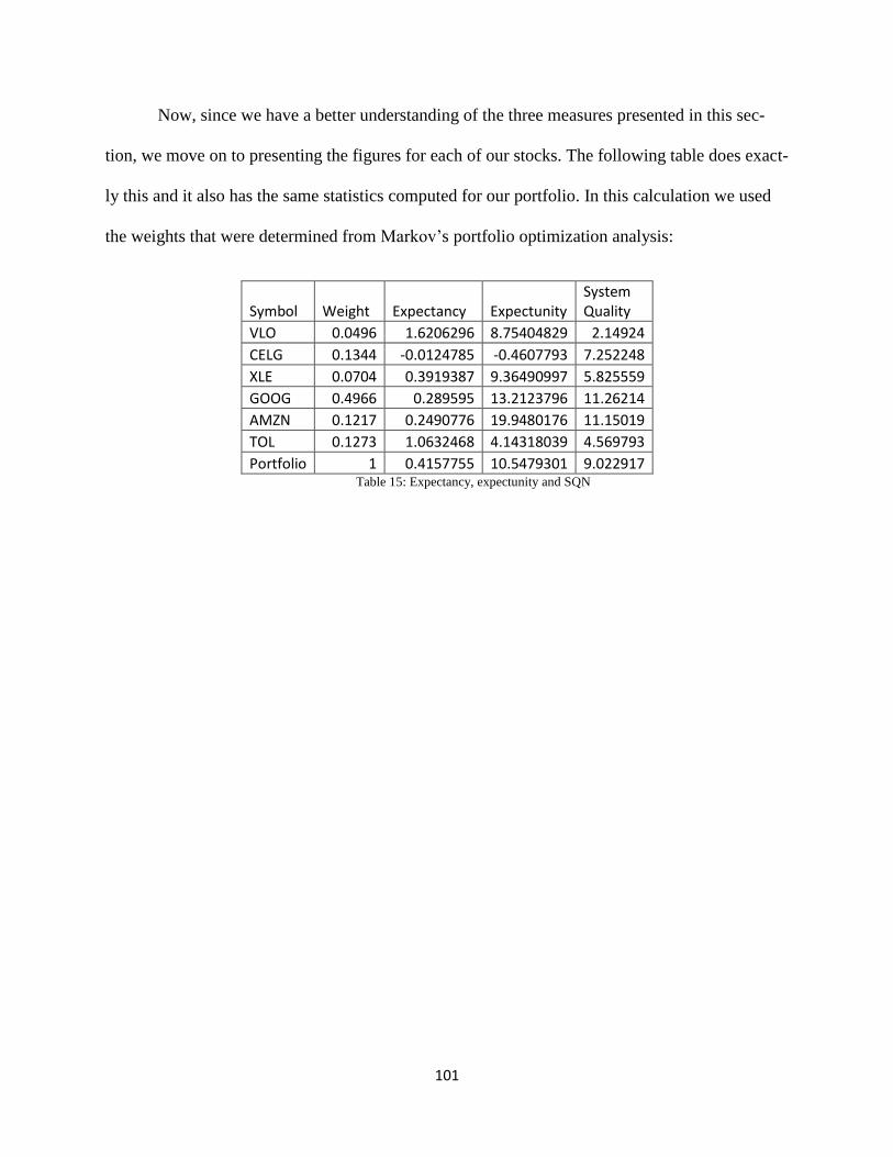
101

Now, since we have a better understanding of the three measures presented in this sec-

tion, we move on to presenting the figures for each of our stocks. The following table does exact-

ly this and it also has the same statistics computed for our portfolio. In this calculation we used

the weights that were determined from Markov’s portfolio optimization analysis:

Symbol Weight Expectancy Expectunity System Quality

VLO 0.0496 1.6206296 8.75404829 2.14924

CELG 0.1344 -0.0124785 -0.4607793 7.252248

XLE 0.0704 0.3919387 9.36490997 5.825559

GOOG 0.4966 0.289595 13.2123796 11.26214

AMZN 0.1217 0.2490776 19.9480176 11.15019

TOL 0.1273 1.0632468 4.14318039 4.569793

Portfolio 1 0.4157755 10.5479301 9.022917 Table 15: Expectancy, expectunity and SQN

102

CHAPTER 7: SUMMARY & CONCLUSIONS

As we have mentioned at the beginning of the paper, our team considers that the more

tests and analysis techniques are applied to an automated strategy, the more confidence the in-

vestor will have to trade it with real money. After all the testing done, we believe that we would

be able to trade the strategy presented in this paper with real money. Our system was developed

such that the different variations of the Precision Trading System that performed the best with

each individual stock over a one-year-long set of data were selected for our final portfolio. Those

selections proved to be robust since they also gave good results over two years’ worth of histori-

cal data.

However, we would have been even surer about our modified PTSs if we would have had

better computing power in order to be able to perform a more thorough optimization and espe-

cially, in order to make the walk forward cluster analysis succeed. Those two analysis techniques

would have possibly pointed us to an even more profitable system.

But the technical difficulties were not the only ones that we encountered. There were also

plenty of implementation challenges and, consequently, our ideas had sometimes to be modified

in order to accustom them to the limitations of EasyLanguage and to the limitations of the

TradeStation account and platform. The team liked the ideas used by the Precision Trading Sys-

tem from the very beginning, but because we wanted to have an edge over other traders that

might also use the strategy, we wanted to make some alterations to it.

At first we tried to use the implied volatility for the options written on the particular stock

that we were trading instead of the standard deviation of the closing prices when computing the

103

upper and lower trend lines. We believed that the volatility would better adapt to the movements

that the price would make88

, but the problem was that the simulated account did not include the

options price feed, and therefore, the volatility couldn’t be calculated.

Secondly, the team wanted to be able to code the quadratic programing strategy used to

determine the weights for our portfolio directly into TradeStation. For this, we would also need

to compute the correlations between our top 20 “Smoothies” at any given moment in time so that

we would know where to invest our capital and how much to invest. The team tried at first load-

ing the 20 symbols in one window in TradeStation, one as a graph and the others as sub-graphs.

The problem was apparent shortly: the platform would get in and out of the market using only

the symbol that was loaded in the first chart. This would beat our purpose of trading multiple

symbols at the same time. Hence, the team decided to load each symbol in a different window

and to try using global variables in order to compute the weights for our portfolio. We are glad

that we realized that the complexity of such an implementation would have been too big to even

back-test it over a reasonable amount of time. We gave up this idea and we decided to use

MATLAB to find the weights for our portfolio.

The third problem encountered was with obtaining our account balance for all the closed

positions at any given moment in time. Unfortunately, as we found out, all the Get functions do

not work in back-testing. Hence, we moved our attention to global variables. Who would have

thought that those variables do not work in back-testing either? We surely didn’t and that is why

we had found it out the hard way. Finally, we stumbled upon the solution: All Data Everywhere

variables.

88

See Ito’s Lemma from page 94

104

Although the project presented us with many intellectual and coding challenges, the de-

sire to answer to the very old question of finding a strategy that makes money gave us motivation

to push even during those hard and, sometimes, frustrating times.

Recommendations

In the future, we would like to try our original idea of using the implied volatility for our

channel and we would like to be able to optimize the strategy and to perform a walk forward

analysis on the strategy over a longer period of time.

As traders like to say, “Trading is an art as much as it is a science”. Hence, some traders

might have other preferences than the ones that our team had. For example, some might want to

choose the smoothies based on more recent data and not on the whole historical prices. If so, we

recommend them to go through choosing the top “Smoothies” and through optimizing their port-

folio periodically. For example, our team decided to run this analysis at least yearly, or every

time we consider that the market conditions changed drastically.

Moreover, we consider that the strategy can accommodate many trading styles. For ex-

ample, by decreasing the number of standard deviations that make up the channel, the strategy

will get in and out of the market more often. The opposite is also true.

Hence, we consider that the Precision Trading System still has a myriad of possibilities

that wait to be discovered. All one needs is imagination and the motivation to uncover them.

105

BIBLIOGRAPHY

All Data Everywhere. (2004, February 12). Retrieved 2013, from TradeStation Forum:

https://community.tradestation.com/Discussions/Topic.aspx?Topic_ID=33398&SearchTe

rm=All%20data%20%20Everywhere&txtExactMatch=

Trading 101: Expectancy. (2004, May 19). Retrieved 2013, from TraderMike:

http://www.tradermike.net/2004/05/trading_101_expectancy/

Macroeconomics - Types of Unemployment. (2009, February 18). Retrieved May 2013, from

Investopedia: http://www.investopedia.com/exam-guide/cfa-level-

1/macroeconomics/unemployment.asp

Overnight Rate. (2009, February 15). Retrieved May 2013, from Investopedia:

http://www.investopedia.com/terms/o/overnightrate.asp

The Basics of Bollinger Bands. (2009, May 13). Retrieved May 2013, from Investopedia:

http://www.investopedia.com/articles/technical/102201.asp

Stock Shastra #29: Learn to read the signals of interest rate and its impact on stock market.

(2010, December 7). Retrieved May 2013, from MoneyWorks4me:

http://stockshastra.moneyworks4me.com/basics-of-investing/stock-shastra-29-learn-to-

read-the-signals-of-interest-rate-and-its-impact-on-stock-market/

The Capital Asset Pricing Model: An Overview. (2010, November 24). Retrieved May 2013,

from Investopedia: http://www.investopedia.com/articles/06/capm.asp

The Utility of Trendlines. (2011, October 14). Retrieved May 2013, from Investopedia:

http://www.investopedia.com/articles/trading/06/trendlines.asp

Channeling: Charting A Path To Success. (2012, May 21). Retrieved May 2013, from

Investopedia: http://www.investopedia.com/articles/trading/05/020905.asp

How Interest Rates Affect The Stock Market. (2012, October 7). Retrieved May 2013, from

Investopedia: http://www.investopedia.com/articles/06/interestaffectsmarket.asp

Robustness of Algorithmic Trading Systems. (2013, April 16). Retrieved 2013, from

VBOsystems: http://www.vbosystems.info/2/post/2013/04/robustness-of-algorithmic-

trading-systems.html

Topic 429 - Traders in Securities. (2013, April 1). Retrieved May 2013, from IRS:

http://www.irs.gov/taxtopics/tc429.html

106

3-Month Treasury Bill: Secondary Market Rate. (n.d.). Retrieved May 2013, from Economic

Research Federal Reserve Bank of St. Louis:

http://research.stlouisfed.org/fred2/series/TB3MS?cid=116

About ProbabilityMap Studies. (n.d.). Retrieved May 2013, from TradeStation Help:

http://help.tradestation.com/09_01/tradestationhelp/pm/about_pm_studies.htm

Average Directional Index (ADX). (n.d.). Retrieved May 2013, from AsiaPacFinance:

http://www.asiapacfinance.com/trading-strategies/technicalindicators/ADX

Average True Range. (n.d.). Retrieved May 2013, from AsiaPacFinance:

http://www.asiapacfinance.com/trading-strategies/technicalindicators/AverageTrueRange

Average True Range - ATR. (n.d.). Retrieved May 2013, from Investopedia:

http://www.investopedia.com/terms/a/atr.asp

Bollinger Bands. (n.d.). Retrieved May 2013, from AsiaPacFinance:

http://www.asiapacfinance.com/trading-strategies/technicalindicators/bollingerbands

Candlestick. (n.d.). Retrieved May 2013, from Investopedia:

http://www.investopedia.com/terms/c/candlestick.asp

Capital Asset Pricing Model - CAPM. (n.d.). Retrieved May 2013, from Investopedia:

http://www.investopedia.com/terms/c/capm.asp

Commodity Channel Index (CCI). (n.d.). Retrieved May 2013, from StockCharts:

http://stockcharts.com/school/doku.php?id=chart_school:technical_indicators:commodity

_channel_ind%20ex_cci

Commodity Channel Index (CCI). (n.d.). Retrieved May 2013, from AsiaPacFinance:

http://www.asiapacfinance.com/trading-

strategies/technicalindicators/CommodityChannelIndex

Competitive Pricing. (n.d.). Retrieved 2013, from TradeStation:

https://www.tradestation.com/pricing

Dow Theory. (n.d.). Retrieved May 2013, from Investopedia:

http://www.investopedia.com/terms/d/dowtheory.asp

Drawdown. (n.d.). Retrieved May 2013, from Investopedia:

http://www.investopedia.com/terms/d/drawdown.asp

Earnings Before Interest, Taxes, Depreciation and Amortization - EBITDA. (n.d.). Retrieved

May 2013, from Investopedia: http://www.investopedia.com/terms/e/ebitda.asp

107

Efficient Market Hypothesis. (n.d.). Retrieved May 2013, from Morningstar:

http://www.morningstar.com/InvGlossary/efficient_market_hypothesis_definition_what_

is.aspx

Fibonacci. (n.d.). Retrieved May 2013, from AsiaPacFinance:

http://www.asiapacfinance.com/trading-strategies/technicalindicators/Fibonacci

Financial Toolbox. (n.d.). Retrieved 2013, from MathWorks:

http://www.mathworks.com/products/finance/description2.html

Gross Profit. (n.d.). Retrieved May 2013, from Investopedia:

http://www.investopedia.com/terms/g/grossprofit.asp

Introduction to Candlesticks. (n.d.). Retrieved May 2013, from StockCharts:

http://stockcharts.com/school/doku.php?id=chart_school:chart_analysis:introduction_to_

candlesticks

Japanese Candlesticks. (n.d.). Retrieved May 2013, from AsiaPacFinance.:

http://www.asiapacfinance.com/trading-strategies/JapaneseCandlesticks

Key Statistics. (n.d.). Retrieved May 2013, from Yahoo! Finance:

http://finance.yahoo.com/q/ks?s=AMZN+Key+Statistics

Langager, C., & Murphy, C. (n.d.). Dow Theory: Market Indexes Must Confirm Each Other.

Retrieved May 2013, from Investopedia:

http://www.investopedia.com/university/dowtheory/dowtheory4.asp

Langager, C., & Murphy, C. (n.d.). Dow Theory: Volume Must Confirm The Trend. Retrieved

May 2013, from Investopedia:

http://www.investopedia.com/university/dowtheory/dowtheory5.asp

Langager, C., & Murphy, C. (n.d.). Dow Theory:Introduction. Retrieved May 2013, from

Investopedia: http://www.investopedia.com/university/dowtheory/

Liberty, J. (2011, August 1). Measuring and avoiding slippage. Retrieved May 2013, from

Futures: http://www.futuresmag.com/2011/08/01/measuring-and-avoiding-slippage

Limit Order. (n.d.). Retrieved May 2013, from Investopedia:

http://www.investopedia.com/terms/l/limitorder.asp

Liquidity. (n.d.). Retrieved May 2013, from Investopedia:

http://www.investopedia.com/terms/l/liquidity.asp

Market Order. (n.d.). Retrieved May 2013, from Investopedia:

http://www.investopedia.com/terms/m/marketorder.asp

108

Meyers, D. (2004). Curve Fitting, Data Mining, Strategy Optimization & Walk Forward

Analysis Using the Acceleration System.

Moving Averages. (n.d.). Retrieved May 2013, from AsiaPacFinance:

http://www.asiapacfinance.com/trading-strategies/technicalindicators/movingaverage

Moving Averages - Simple and Exponential. (n.d.). Retrieved May 2013, from StockCharts:

http://stockcharts.com/school/doku.php?id=chart_school:technical_indicators:moving_av

erages

Operating Margin. (n.d.). Retrieved May 2013, from Investopedia:

http://www.investopedia.com/terms/o/operatingmargin.asp

Options Basics:What Are Options? (n.d.). Retrieved May 2013, from Investopedia:

http://www.investopedia.com/university/options/option.asp

Pivot Points. (n.d.). Retrieved May 2013, from StockCharts:

http://stockcharts.com/help/doku.php?id=chart_school:technical_indicators:pivot_points

Pivot Points. (n.d.). Retrieved May 2013, from AsiaPacFinance:

http://www.asiapacfinance.com/trading-strategies/technicalindicators/pivotpoints

Price Channels. (n.d.). Retrieved May 2013, from StockCharts:

http://stockcharts.com/school/doku.php?id=chart_school:technical_indicators:price_chan

nels

Price-Earnings Ratio - P/E Ratio. (n.d.). Retrieved May 2013, from Investopedia:

http://www.investopedia.com/terms/p/price-earningsratio.asp

Profit Margin. (n.d.). Retrieved May 2013, from Investopedia:

http://www.investopedia.com/terms/p/profitmargin.asp

Raiman, M. (n.d.). Retrieved 2013, from PTS Precision Trading System:

http://www.precisiontradingsystem.com/AboutTheCourse.html

Raiman, M. (n.d.). About PTS.

Random Walk Index. (n.d.). Retrieved May 2013, from AsiaPacFinance:

http://www.asiapacfinance.com/trading-strategies/technicalindicators/RandomWalkIndex

Relative Strength Index (RSI). (n.d.). Retrieved May 2013, from AsiaPacFinance:

http://www.asiapacfinance.com/trading-

strategies/technicalindicators/RelativeStrengthIndex

Return on Assets - ROA. (n.d.). Retrieved May 2013, from Investopedia:

http://www.investopedia.com/terms/r/returnonassets.asp

109

Revenue. (n.d.). Retrieved May 2013, from Investopedia:

http://www.investopedia.com/terms/r/revenue.asp

Risk Premium. (n.d.). Retrieved May 2013, from Investopedia:

www.investopedia.com/terms/r/riskpremium.asp

Ruppert, D. (2011). Statistics and Data Analysis for Financial Engineering. Springer.

RWI - Random Walk Index. (n.d.). Retrieved May 2013, from eTrading:

http://www.etrading.sk/en/technical-analysis/44-indikatory-technickej-analyzy/168-rwi-

random-walk-index

Sharpe Ratio. (n.d.). Retrieved May 2013, from Investopedia:

http://www.investopedia.com/terms/s/sharperatio.asp

Skousen, M. (2006, February 6). Inflation's Effect on the Stock Market: Why Good News is Bad

News on Wall Street. Retrieved May 2013, from InvestmentU:

http://www.investmentu.com/2006/February/impact-of-inflation-on-stock-market.html

Spicer, J., & Younglai, R. (2010, October 1). Single trade helped spark May's flash crash.

Retrieved May 2013, from Reuters: http://www.reuters.com/article/2010/10/02/us-flash-

idUSTRE69040W20101002

Stock-Picking Strategies: CAN SLIM. (n.d.). Retrieved May 2013, from Investopedia:

http://www.investopedia.com/university/stockpicking/stockpicking7.asp

Stocks Basics:What Are Stocks? (n.d.). Retrieved May 2013, from Investopedia:

http://www.investopedia.com/university/stocks/stocks1.asp

Stop Order. (n.d.). Retrieved May 2013, from Investopedia:

http://www.investopedia.com/terms/s/stoporder.asp

Trend Lines. (n.d.). Retrieved May 2013, from StockCharts:

http://stockcharts.com/school/doku.php?id=chart_school:chart_analysis:trend_lines

Unemployment Rate. (n.d.). Retrieved May 2013, from Investopedia:

http://www.investopedia.com/terms/u/unemploymentrate.asp

Volume. (n.d.). Retrieved May 2013, from Investopedia:

http://www.investopedia.com/terms/v/volume.asp

What Is a Bond? (n.d.). Retrieved May 2013, from The Wall Street Journal:

http://guides.wsj.com/personal-finance/investing/what-is-a-bond/

Wright, C. (n.d.). Trading as a Business.

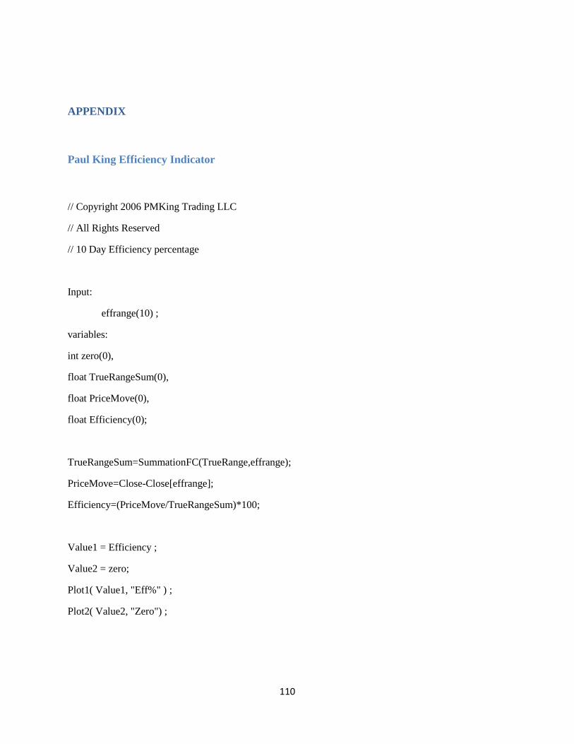
110

APPENDIX

Paul King Efficiency Indicator

// Copyright 2006 PMKing Trading LLC

// All Rights Reserved

// 10 Day Efficiency percentage

Input:

effrange(10) ;

variables:

int zero(0),

float TrueRangeSum(0),

float PriceMove(0),

float Efficiency(0);

TrueRangeSum=SummationFC(TrueRange,effrange);

PriceMove=Close-Close[effrange];

Efficiency=(PriceMove/TrueRangeSum)*100;

Value1 = Efficiency ;

Value2 = zero;

Plot1( Value1, "Eff%" ) ;

Plot2( Value2, "Zero") ;

111

Adapted Paul King Efficiency Indicator

// 10 Day Efficiency percentage

Input:

effrange (10),

avgeffrange (100);

variables:

int zero(0),

float TrueRangeSum(0),

float PriceMove(0),

float Efficiency(0);

TrueRangeSum=SummationFC(TrueRange,effrange);

PriceMove=Close-Close[effrange];

Efficiency=(PriceMove/TrueRangeSum)*100;

Value1 = Average(Efficiency,avgeffrange);

Commentary("Efficiency=", Value1);

112

Correlation Matrix for the “Smoothies”

Table 16: Correlation matrix

MATLAB Code for Portfolio Optimization

The following function taxes as inputs the risk free rate, the mean vector and correlation

matrix for the “Smoothies” and outputs the weights for the Markov optimized portfolio and a

plot of the risk vs return for our portfolio:

function [ weights ] = MaxSharpeRatioPortfolio( risk_free ) %UNTITLED Summary of this function goes here % Detailed explanation goes here mu=xlsread('Mean&stdev for Smoothies.xlsx','mu'); sigma=xlsread('Mean&stdev for Smoothies.xlsx','Covariance matrix'); p=Portfolio('AssetMean',mu,'AssetCovar',sigma,'RiskFreeRate',risk_free); p=p.setDefaultConstraints; weights=p.estimateMaxSharpeRatio; [risk, ret]=p.estimatePortMoments(weights); hold on plot(risk,ret,'*r'); end

VLO CELG GS XLE AAPL GOOG CVX LVS SLB IWM AMZN BBRY QCOM XOM CAT MDT TOL MS IYR IBM

VLO 1

CELG 0.157026 1

GS 0.325034 0.226984 1

XLE 0.612816 -0.01913 0.423097 1

AAPL 0.086437 0.15991 0.351472 0.28591 1

GOOG 0.130271 0.037273 0.476826 0.385779 0.526536 1

CVX 0.34514 0.015421 0.219313 0.667109 0.185973 0.087977 1

LVS 0.356677 0.122437 0.49255 0.437396 0.317916 0.345689 0.243067 1

SLB 0.443798 0.141997 0.463114 0.702968 0.160675 0.268212 0.40295 0.426812 1

IWM 0.324617 0.201226 0.545386 0.480737 0.390799 0.298522 0.285842 0.52758 0.428589 1

AMZN 0.187443 0.270747 0.282055 0.234871 0.346591 0.256117 0.230263 0.288242 0.18848 0.394631 1

BBRY 0.275852 0.414138 0.409891 0.253978 0.227073 0.338952 -0.00103 0.440522 0.416828 0.428088 0.291055 1

QCOM 0.180847 0.242549 0.265632 0.227581 0.163288 0.282919 0.187001 0.363536 0.214094 0.410254 0.293431 0.377811 1

XOM 0.314669 0.058028 0.163655 0.604468 0.142661 0.229693 0.463764 0.184497 0.326456 0.255866 0.172752 0.14925 0.162016 1

CAT 0.246286 -0.01888 0.397179 0.538557 0.188449 0.199572 0.26105 0.503903 0.389051 0.492952 0.077142 0.133062 0.187689 0.21602 1

MDT 0.199604 0.107546 0.208344 0.303025 0.150736 0.289434 0.079687 0.405409 0.182427 0.38561 0.107081 0.269581 0.091209 0.074837 0.253468 1

TOL 0.098194 0.096245 0.26772 0.221347 0.152273 0.164137 0.131703 0.276105 0.06664 0.320833 0.052925 0.109571 0.109097 0.147823 0.274196 0.179285 1

MS 0.321623 0.142816 0.752123 0.409036 0.224767 0.376912 0.237532 0.37355 0.287967 0.517665 0.27396 0.36026 0.258195 0.162904 0.264068 0.164155 0.292139 1

IYR 0.204779 0.094248 0.387857 0.309754 0.219087 0.289193 0.193051 0.652461 0.285015 0.80143 0.189139 0.283866 0.303496 0.158754 0.435534 0.378389 0.326779 0.342523 1

IBM 0.229809 0.060448 0.456532 0.341161 0.33059 0.298125 0.205511 0.450483 0.258884 0.466496 0.446674 0.250381 0.234795 0.190721 0.254804 0.18228 0.102938 0.325465 0.265744 1

113

Overview of the selected stocks89

Valero Energy Corporation (VLO)

Valero is a petroleum and gas company that refines, distributes and markets the

resources. This company should do well especially when the economy is not doing well because

energy is the last one that people would want to cut spending on.

Celgene Corporation (CELG)

Celgene is a biotechnology company that researches and distributes products for the

treatment of cancer and inflammatory diseases. Just like any technology company, CELG should

do well when the economy is doing well and it should also be doing well when the economy is

recovering from a recession. This is because technology companies tend to invest more of their

profits in research and development and it is this prospect that also attracts investors.

Energy Select Sector SPDR (XLE)

As the name suggests, XLE is an equity energy fund. Just like VLO, this ETF should

perform well during economic uncertainty, hedging our risk even more.

Google (GOOG) and Amazon (AMZN)

Just like Celgene, the two big technology companies should perform well when the

economy also performs well and it should be some of the first stocks that would pick up the

slightest headwind during economic recovery.

89

Yahoo Finance < http://finance.yahoo.com>

114

Toll Brothers (TOL)

Toll Brothers is a residential construction company, with a main focus on luxury homes.

This company should do very well during economic growth and very poorly during economic

downturn.

The Basic PTS Strategy EasyLanguage code

inputs:

StartingBalance ( 350000 ),

Length ( 23 ), { // Length of Linear Regression // }

Weight ( 0.0496 ), { // The weight that VLO has in our portfolio //}

SlopeUp_Data2 ( 0.05 ), { // The positive slope on the 15 minute bar timeline //}

SlopeDn_Data2 ( -0.05 ), { // The negative slope on the 15 minute bar timeline //}

SlopeUp_Data3 ( 0.05 ), { // The positive slope on the 30 minute bar timeline //}

SlopeDn_Data3 ( -0.05 ), { // The negative slope on the 30 minute bar timeline //}

Size ( 2 ), {//Trend Line Thickness //}

NumDevsUp ( 1 ), { // Standard deviations for upper band // }

NumDevsDn ( -1 ), { // Standard deviations for lower band // }

LRColor ( Yellow ), { // Color for Linear Regression Line // }

LBColor ( Magenta ), { // Color for Lower Boundary Line // }

UBColor ( Blue ), { // Color for the Upper Boundary Line //}

ExtRight ( false ), { // Set to true to extend to right // }

ExtLeft ( false ); { // Set to true to extend to left // }

variables:

Class ("Profit"),

InfoMap1 (MapSN.New),

115

ProfitSoFar ( 0 ),

ProfitSoFar1 ( 0 ),

ProfitSoFar2 ( 0 ),

ProfitSoFar3 ( 0 ),

ProfitSoFar4 ( 0 ),

ProfitSoFar5 ( 0 ),

ProfitSoFar6 ( 0 ),

AccBalance ( 0 ),

NrShares ( 0 ),

FirstDate_Data1 ( 0 ),



FirstTime_Data1 ( 0 ),



UpperBand_Data1 ( 0 ),

LowerBand_Data1 ( 0 ),

UpperBand_1_Data1 ( 0 ),

LowerBand_1_Data1 ( 0 ),

LRV_Data1 ( 0 ),

LRV_Data2 ( 0 ),

LRV_Data3 ( 0 ),

LRV_1_Data1 ( 0 ),

LRV_1_Data2 ( 0 ),

LRV_1_Data3 ( 0 ),

TL_LRV_Data1 ( 0 ),

TL_LRV_Data2 ( 0 ),

TL_LRV_Data3 ( 0 ),

TL_UB_Data1 ( 0 ),

116

TL_UB_Data2 ( 0 ),

TL_LB_Data1 ( 0 ),

TL_LB_Data2 ( 0 ),

Flag ( 0 ),

TL_UB_Value_Data1 ( 0 ),

TL_UB_Value_Data2 ( 0 ),

TL_LB_Value_Data1 ( 0 ),

TL_LB_Value_Data2 ( 0 ),

TL_Slope_Data1 ( 0 ),



SDev_Data1 ( 0 ),

SDev_Data2 ( 0 );











117



SDev_Data1 = StandardDev( Close of Data1, Length, 1 ) of Data1;

UpperBand_Data1 = LRV_Data1 + NumDevsUp * SDev_Data1;

LowerBand_Data1 = LRV_Data1 + NumDevsDn * SDev_Data1;

UpperBand_1_Data1 = LRV_1_Data1 + NumDevsUp * SDev_Data1;

LowerBand_1_Data1 = LRV_1_Data1 + NumDevsDn * SDev_Data1;

TL_LRV_Data1 = TL_New( FirstDate_Data1, FirstTime_Data1, LRV_1_Data1, date, time,

LRV_Data1 ) of Data1;





TL_UB_Data1 = TL_New( FirstDate_Data1, FirstTime_Data1, UpperBand_1_Data1, date, time,

UpperBand_Data1 ) of Data1;

TL_LB_Data1 = TL_New( FirstDate_Data1, FirstTime_Data1, LowerBand_1_Data1, date, time,

LowerBand_Data1 ) of Data1;

TL_SetColor( TL_LRV_Data1, LRColor );



TL_SetColor( TL_UB_Data1, UBColor );

TL_SetColor( TL_LB_Data1, LBColor );

TL_SetSize(TL_LRV_Data1, size);



TL_SetSize(TL_UB_Data1, size);

118

TL_SetSize(TL_LB_Data1, size);

TL_SetExtLeft( TL_LRV_Data1, ExtLeft );



TL_SetExtLeft( TL_UB_Data1, ExtLeft );

TL_SetExtLeft( TL_LB_Data1, ExtLeft );

TL_SetExtRight( TL_LRV_Data1, ExtRight );



TL_SetExtRight( TL_UB_Data1, ExtRight );

TL_SetExtRight( TL_LB_Data1, ExtRight );

TL_SetBegin( TL_LRV_Data1, FirstDate_Data1, FirstTime_Data1, LRV_1_Data1 );



TL_SetBegin( TL_UB_Data1, FirstDate_Data1, FirstTime_Data1, UpperBand_1_Data1 );

TL_SetBegin( TL_LB_Data1, FirstDate_Data1, FirstTime_Data1, LowerBand_1_Data1 );

TL_SetEnd( TL_LRV_Data1, date, time, LRV_Data1 );



TL_SetEnd( TL_UB_Data1, date, time, UpperBand_Data1 );

TL_SetEnd( TL_LB_Data1, date, time, LowerBand_Data1 );

TL_UB_Value_Data1 = TL_GetValue(TL_UB_Data1, Date, Time);

TL_LB_Value_Data1 = TL_GetValue(TL_LB_Data1, Date, Time);

119



Value1=ADE.OpenMap (Class, "VLO", ADE.BarInterval);

Value1=ADE.GetBarInfo (Class, "VLO", ADE.BarInterval, ADE.BarID, InfoMap1);


Value2=ADE.OpenMap(Class, "CELG", ADE.BarInterval);

Value2=ADE.GetBarInfo (Class, "CELG", ADE.BarInterval, ADE.BarID, InfoMap1);


Value3=ADE.OpenMap(Class, "XLE", ADE.BarInterval);

Value3=ADE.GetBarInfo (Class, "XLE", ADE.BarInterval, ADE.BarID, InfoMap1);


Value4=ADE.OpenMap(Class, "GOOG", ADE.BarInterval);

Value4=ADE.GetBarInfo (Class, "GOOG", ADE.BarInterval, ADE.BarID, InfoMap1);


Value5=ADE.OpenMap(Class, "AMZN", ADE.BarInterval);

Value5=ADE.GetBarInfo (Class, "AMZN", ADE.BarInterval, ADE.BarID, InfoMap1);


Value6=ADE.OpenMap(Class, "TOL", ADE.BarInterval);

Value6=ADE.GetBarInfo (Class, "TOL", ADE.BarInterval, ADE.BarID, InfoMap1);


AccBalance=(ProfitSoFar1+ProfitSoFar2+ProfitSoFar3+ProfitSoFar4+ProfitSoFar5+ProfitSoFar

6+StartingBalance)*Weight;

120

NrShares=floor(AccBalance/close);




Else


TL_Slope_Data3 >= SlopeUp_Data3 and marketposition = 0 then Buy ("Close>UB 2") NrShares shares

next bar at market; {TL_LB_Value limit}




Else


TL_Slope_Data3 <= SlopeDn_Data3 and marketposition=0 then Sell short NrShares shares next bar at

market;



buy to cover next bar at market

Else


TL_Slope_Data3 >= SlopeUp_Data3 and marketposition = 0 then buy NrShares shares next bar at

market;



Sell ("Close<LB 1") all contracts next bar at market

Else


TL_Slope_Data3 <= SlopeDn_Data3 and marketposition = 0 then sell short ("Close<LB 2") NrShares

shares next bar at market;

121

Commentary( "TL_Slope_Data2=", TL_Slope_Data2, Newline,

"TL_Slope_Data3=", TL_Slope_Data3, Newline,

"Account Balance=", AccBalance, Newline,

"Number of Shares=", NrShares, Newline,

"Profit 1=", ProfitSoFar1,Newline,





"Profit 6=", ProfitSoFar6, Newline)

Strategy that Loads the Net Profit into an ADE

Vars:

Class ("Profit"),

InfoMap1 (MapSN.New);

If Getsymbolname="VLO" then

Begin

Value1 = MapSN.Put (InfoMap1, "ProfitSoFar1", Netprofit);

Value1 = ADE.PutBarInfo (Class, "VLO", ADE.BarInterval , ADE.BarID, InfoMap1);

End;

If Getsymbolname="CELG" then

Begin


Value2=ADE.PutBarInfo (Class, "CELG", ADE.BarInterval, ADE.BarID, InfoMap1);

End;

122

If Getsymbolname="XLE" then

Begin


Value3=ADE.PutBarInfo (Class, "XLE", ADE.BarInterval , ADE.BarID, InfoMap1);

End;

If Getsymbolname="GOOG" then

Begin


Value4=ADE.PutBarInfo (Class, "GOOG", ADE.BarInterval , ADE.BarID, InfoMap1);

End;

If Getsymbolname="AMZN" then

Begin


Value5=ADE.PutBarInfo (Class, "AMZN", ADE.BarInterval , ADE.BarID, InfoMap1);

End;

If Getsymbolname="TOL" then

Begin


Value6=ADE.PutBarInfo (Class, "TOL", ADE.BarInterval , ADE.BarID, InfoMap1);

End;

123

Performance Report for the Strategy before Optimization


Figure 7: Performance report for VLO

124


Figure 8: Performance report for CELG

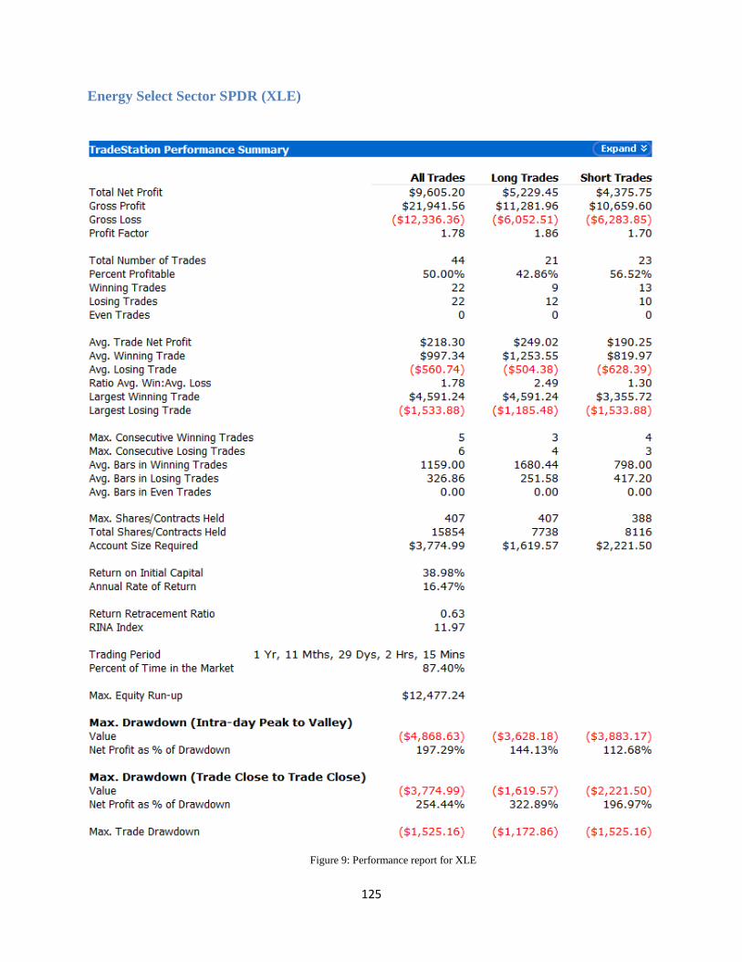
125


Figure 9: Performance report for XLE

126

Google (GOOG)

Figure 10: Performance report for GOOG

127

Amazon (AMZN)

Figure 11: Performance report for AMZN

128

Toll Brothers (TOL)

Figure 12: Performance report for TOL

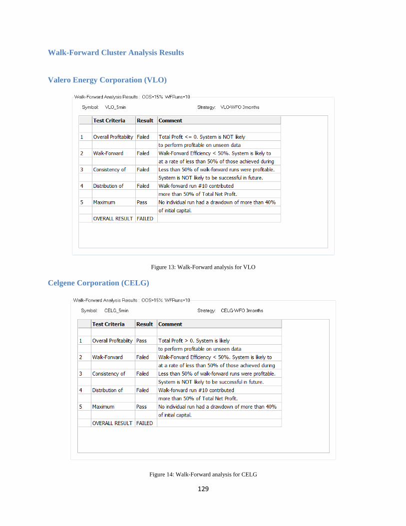
129

Walk-Forward Cluster Analysis Results


Figure 13: Walk-Forward analysis for VLO


Figure 14: Walk-Forward analysis for CELG

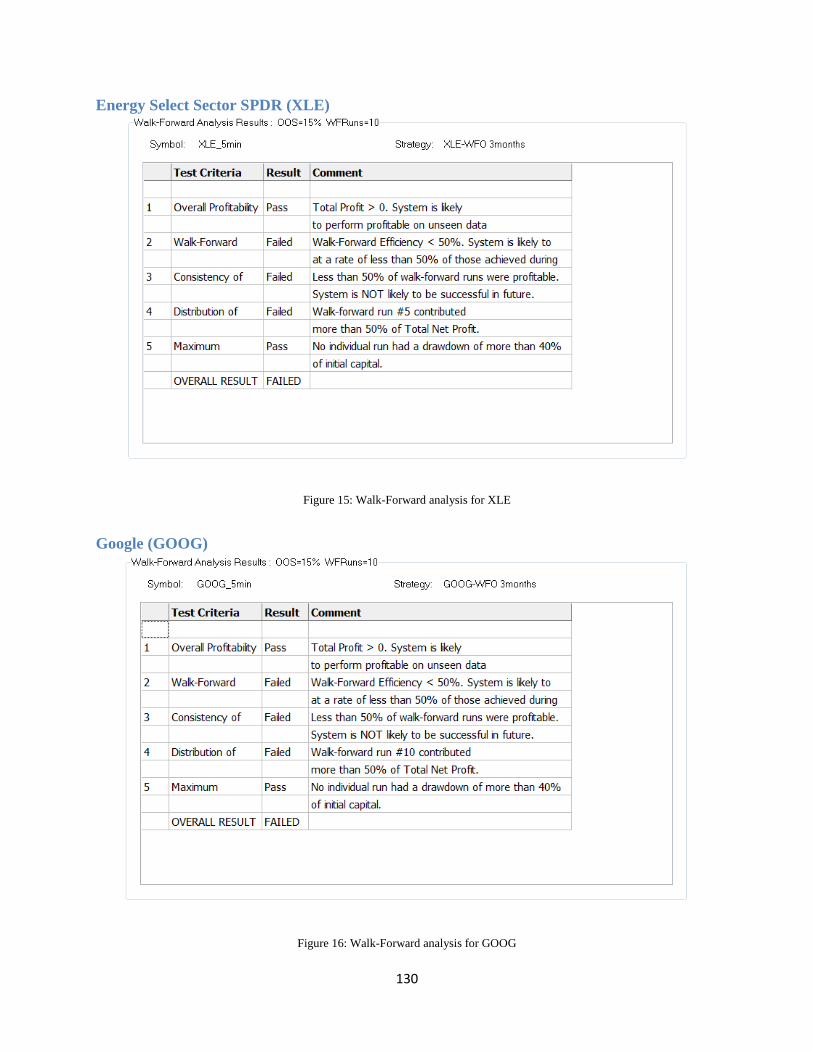
130


Figure 15: Walk-Forward analysis for XLE

Google (GOOG)

Figure 16: Walk-Forward analysis for GOOG

131

Amazon (AMZN)

Figure 17: Walk-Forward analysis for AMZN

Toll Brothers (TOL)

Figure 18: Walk-Forward analysis for TOL

132

Equity Curves


Figure 19: Equity curve for VLO


Figure 20: Equity curve for CELG

133


Figure 21: Equity curve for XLE

Google (GOOG)

Figure 22: Equity curve for GOOG

134

Amazon (AMZN)

Figure 23: Equity curve for AMZN

Toll Brothers (TOL)

Figure 24: Equity curve for TOL

automating the precision trading system

Documents