automatic synthesis using genetic programming of an improved general-purpose controller for...
TRANSCRIPT
Automatic Synthesis Using Genetic Programming of an Improved General-Purpose Controller for
Industrially Representative Plants
Martin A. Keane
Econometrics, Inc.
Chicago, [email protected]
John R. Koza
Stanford University
Stanford, [email protected]
Matthew J. Streeter
Genetic Programming, Inc.
Mountain View, [email protected]
Evolvable Hardware 2002, Washington D.C., July 15-18

Overview
• The problem of industrial control
• P, PI, and PID controllers
• The Astrom-Hagglund controller
• Genetic programming and control
• Evolved controllers
• Cross-validation
• Conclusions

The problem of industrial control
• Example: cruise control
• Desired speed is reference signal
• Flow of fuel to engine is control signal
• Engine/car is plant; car’s speed is plant response

Evaluating Controllers
• Low rise time: the plant response must rise to the desired value quickly
• Minimal overshoot: the plant response must not rise too far above the desired value
• Stability: controller should be stable with respect to noise in the feedback signals
• Sensitivity: controller should not be overly sensitive to small changes in reference signal or plant response
• Disturbance rejection: the controller must work even if its own output is offset by external forces

P, PI, and PID Controllers
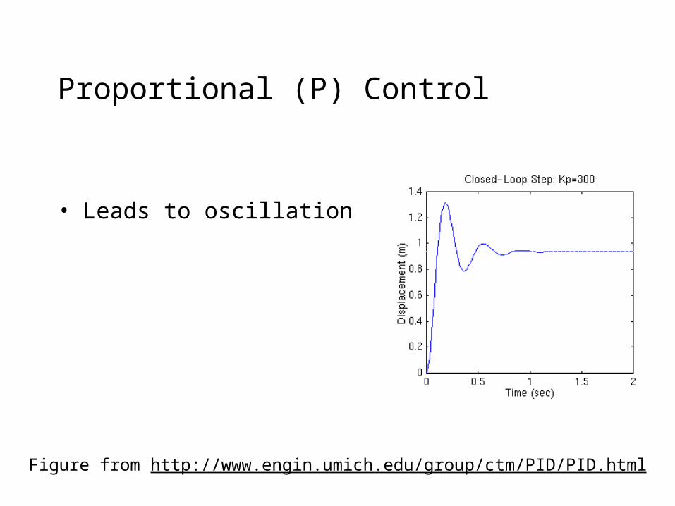
Proportional (P) Control
• Leads to oscillation
Figure from http://www.engin.umich.edu/group/ctm/PID/PID.html

Proportional-Integrative (PI) Control
• Eliminates oscillation
• Doesn’t anticipate future values of plant response
Figure from http://www.engin.umich.edu/group/ctm/PID/PID.html

Proportional-Integrative-Derivative (PID) Control
• With appropriate tuning, outperforms both P and PI controllers
• Over 90% of modern controllers are PID
Figure from http://www.engin.umich.edu/group/ctm/PID/PID.html

Tuning rules for PID controllers
• Original PID controllers were tuned manually
• Ziegler-Nichols (1942) provided generalized tuning equations
• Astrom-Hagglund (1995) Applied curve-fitting to values obtained by well-known “dominant pole design” to obtain improved generalized tuning rules

The Astrom-Hagglund Controller
• Applied “dominant pole design” to 16 plants from 4 representative families of plants
• Used curve-fitting to obtain generalized solution
• Equations are expressed in terms of ultimate gain (Ku), ultimate period (Tu), time constant (Tr) and dead time (L), all readily obtainable in the field
• Broadly recognized and accepted in the control world
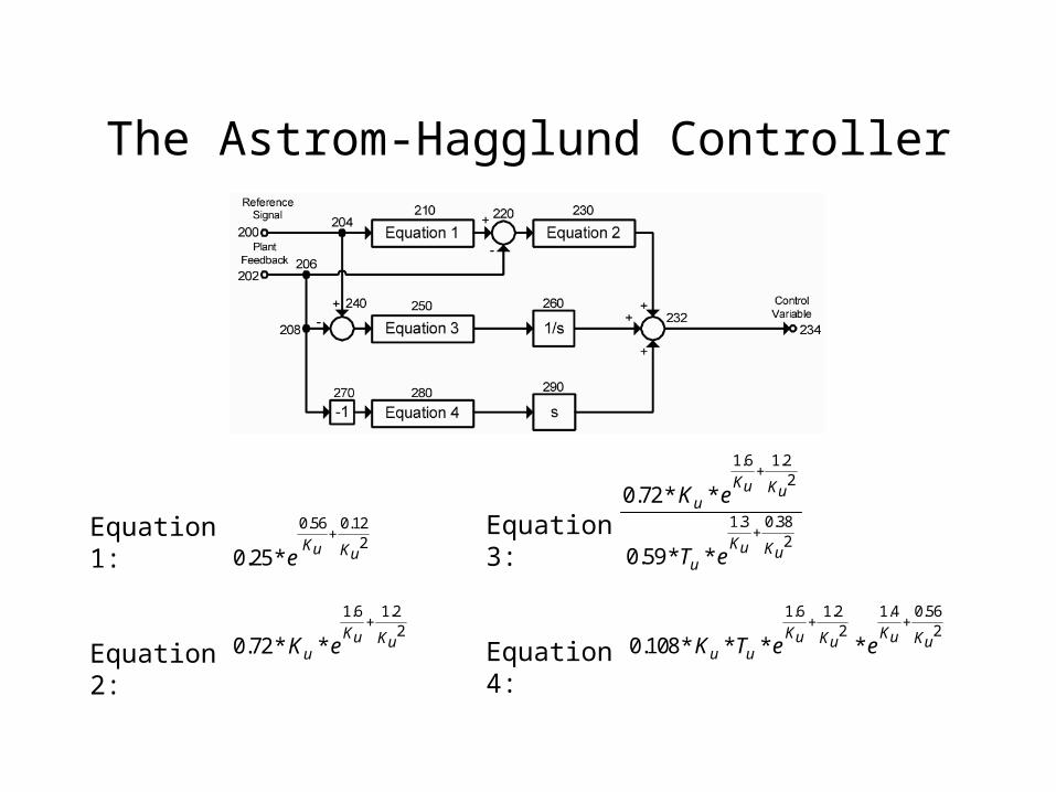
The Astrom-Hagglund Controller
Equation 1:
Equation 2:
0.56 0.12+ 2
0.25*Ku Kue
1.6 1.2+
20.72* *
Ku KuuK e
1.6 1.2+ 2
1.3 0.38+ 2
0.72* *
0.59* *
Ku Kuu
Ku Kuu
K e
T e
1.6 1.2 1.4 0.56+ +
2 20.108* * * *
K Ku uK Ku uu uK T e e
Equation 3:
Equation 4:

Genetic Programming and Control
• Controllers are represented as LISP expression trees
• Crossover is performed by swapping subtrees
• Evolution of topology, identity of each block, and equations giving parameter values of blocks
• Fitness incorporates rise time, overshoot, and disturbance rejection (ITAE), stability, and sensitivity
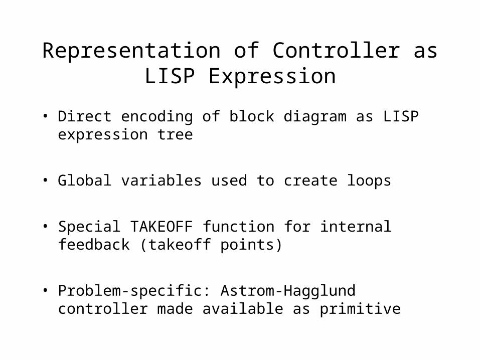
Representation of Controller as LISP Expression
• Direct encoding of block diagram as LISP expression tree
• Global variables used to create loops
• Special TAKEOFF function for internal feedback (takeoff points)
• Problem-specific: Astrom-Hagglund controller made available as primitive

Representation of Controller as LISP Expression

Fitness Measure
• ITAE penalty (Integral of time-weighted absolute error) for setpoint and disturbance rejection
• Penalty for minimum sensor noise attenuation (sensitivity)
• Penalty for maximum sensitivity to noise (stability)
• Evaluation on 20-24 plants, always including 16 Astrom-Hagglund plants

ITAE Penalty
Reference signal Disturbance signal
1.0 1.0
10-3 10-3
-10-6 10-6
1.0 -0.6
-1.0 0.0
0.0 1.0
Six combinations of reference and
disturbance signal heights
22
20
10
10
0
)()10()(
u
u
u
u
u
T
T
Ttu
T
T
t
CdtteTtBdttet
• Penalty is given by:
• B and C are normalizing factors

Stability Penalty
• 0 reference signal, 1 V noise signal
• Maximum sensitivity is maximum amplitude of noise signal + plant response
• Penalty is 0 if Ms < 1.5
2(Ms-1.5) if 1.5 Ms 2.0
20(Ms-1.0) is Ms > 2.0

Sensitivity Penalty
• 0 reference signal, 1 V noise signal
• Amin is minimum attenuation of plant response
• Penalty is 0 if Amin > 40 db
(40-Amin)/10 if 20 db Amin 40 db
2+(20-Amin) if Amin < 20 db

Simulation
• Evolved controllers simulated with SPICE circuit simulator using user-defined control blocks
• 160 or 192 simulations per individual

Previous Work
• Controllers for two and three lag plants
• Discovery of PID and PID2 controllers
• Controller for highly non-linear plant
• Generalized controller for three lag plant with variable time constant
• Generalized controller for two families of plants
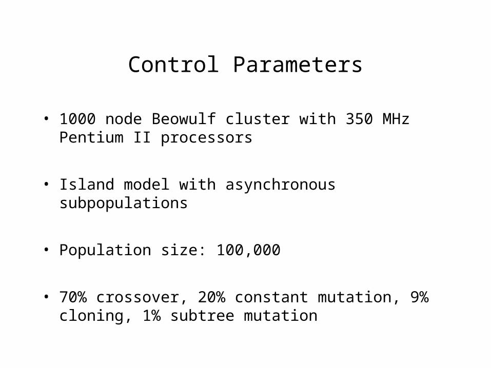
Control Parameters
• 1000 node Beowulf cluster with 350 MHz Pentium II processors
• Island model with asynchronous subpopulations
• Population size: 100,000
• 70% crossover, 20% constant mutation, 9% cloning, 1% subtree mutation

Evolved Controllers

Block Diagram for First Evolved Controller
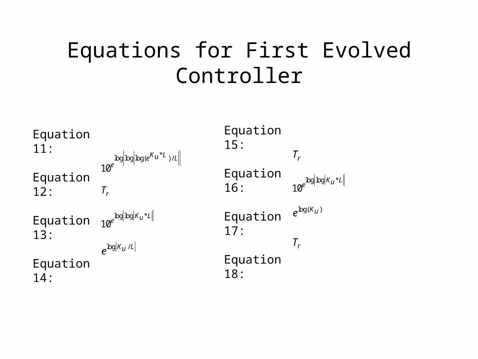
Equations for First Evolved Controller
Equation 11: Equation 12:
Equation 13:
Equation 14:
*log log log( ) /
10
K Lue Le
rT
log log *10
K Lue
log /K Lue
Equation 15: Equation 16:
Equation 17:
Equation 18:
rT
log log *10
K Lue
log( )Kue
rT

Performance of First Evolved Controller
• 66.4% of setpoint ITAE of A-H controller
• 85.7% of disturbance rejection ITAE of A-H controller
• 94.6% of 1/(minimum attenuation) of A-H controller
• 92.9% of maximum sensitivity of A-H controller

Block Diagram for Second Evolved
Controller

Equations for Second Evolved Controller
Equation 21:
Equation 22:
Equation 23:
Equation 24:
Equation 25: Equation 26:
Equation 27:
Equation 28:
log 2 + Lr uT K
( )( )
0.68631( )
1- -
0.13031
- -
log log +
^1
- -0.69897
++ ^^abs(log(abs( + ^ )))
LT Tr u
LTu LK Tu uLKuT Kr u
KuLT Tr u
LT Kr uT Kr uKur uT K
log +log 2 +
LT Kr ur uT K
log + Lr uT K
( )log + log +1.2784r rT T
( )( )log log ^log + +L
K Lur rT T x
log log += +
LT Kr ur ux T K
( )log + +LL
r r uT T K
log 2 + Lr uT K

Performance of Second Evolved Controller
• 85.5% of setpoint ITAE of A-H controller
• 91.8% of disturbance rejection ITAE of A-H controller
• 98.9% of 1/(minimum attenuation) of A-H controller
• 97.5% of maximum sensitivity of A-H controller

Block Diagram for Third Evolved Controller

Equations for Third Evolved Controller
Equation 31: Equation 32:
Equation 33:
Equation 34:
( )loglog - + log
+1
L
r uu
LT T
T
( ) ( )( )2 3NLM log - abs( ) +1 - 2L L Lu u r uL L T T T e T e
( )( )( )NLM log - 2 2 log - log +L L Lu u u u uL T e K K e L T K e
log +1rT
NLM(x) = 100 if x < -100 or x > 10010(-100/19-x/19) if -100 x < -510(100/19-x/19) if 5 < x 10010x if -5 x 5
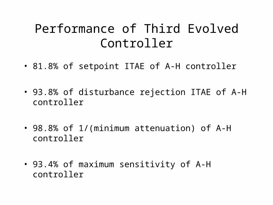
Performance of Third Evolved Controller
• 81.8% of setpoint ITAE of A-H controller
• 93.8% of disturbance rejection ITAE of A-H controller
• 98.8% of 1/(minimum attenuation) of A-H controller
• 93.4% of maximum sensitivity of A-H controller

Comparison of Response of Evolved Controller and Astrom-Hagglund Controller
for a Typical Plant
• Evolved controller has shorter rise time and less overshoot
• Comparison is similar for other plants

Cross-Validation
• 18 new plants selected with plant parameters in range specified by Astrom and Hagglund
• All evolved controllers do better than Astrom-Hagglund controller over 18 additional plants
• Evolved controllers outperform Astrom-Hagglund controller on out-of-sample fitness cases about 99% of the time

Cross-Validation of First Evolved Controller
• 64.1% of setpoint ITAE of A-H controller
• 84.9% of disturbance rejection ITAE of A-H controller
• 95.8% of 1/(minimum attenuation) of A-H controller
• 93.5% of maximum sensitivity of A-H controller

Cross-Validation of Second Evolved Controller
• 84% of setpoint ITAE of A-H controller
• 90.6% of disturbance rejection ITAE of A-H controller
• 98.9% of 1/(minimum attenuation) of A-H controller
• 97.5% of maximum sensitivity of A-H controller

Cross-Validation of Third Evolved Controller
• 81.8% of setpoint ITAE of A-H controller
• 94.2% of disturbance rejection ITAE of A-H controller
• 99.7% of 1/(minimum attenuation) of A-H controller
• 92.5% of maximum sensitivity of A-H controller

Conclusions
• Genetic programming can provide a generalized controller for a wide variety of industrially representative plants
• Significant improvement over Astrom-Hagglund controller as measured by ITAE for setpoint and disturbance rejection, minimum attenuation, and maximum sensitivity
• Evolved controller performs well on out-of-sample plants