automatic speech emotion recognition using …...automatic speech emotion recognition using...

Available online at www.sciencedirect.com

www.elsevier.com/locate/specom

Speech Communication 53 (2011) 768–785

Automatic speech emotion recognition usingmodulation spectral features

Siqing Wu a,⇑, Tiago H. Falk b, Wai-Yip Chan a

a Department of Electrical and Computer Engineering, Queen’s University, Kingston, ON, Canada K7L 3N6b Institute of Biomaterials and Biomedical Engineering, University of Toronto, Toronto, ON, Canada M5S 3G9

Available online 7 September 2010

Abstract

In this study, modulation spectral features (MSFs) are proposed for the automatic recognition of human affective information fromspeech. The features are extracted from an auditory-inspired long-term spectro-temporal representation. Obtained using an auditory filt-erbank and a modulation filterbank for speech analysis, the representation captures both acoustic frequency and temporal modulationfrequency components, thereby conveying information that is important for human speech perception but missing from conventionalshort-term spectral features. On an experiment assessing classification of discrete emotion categories, the MSFs show promising perfor-mance in comparison with features that are based on mel-frequency cepstral coefficients and perceptual linear prediction coefficients, twocommonly used short-term spectral representations. The MSFs further render a substantial improvement in recognition performancewhen used to augment prosodic features, which have been extensively used for emotion recognition. Using both types of features, anoverall recognition rate of 91.6% is obtained for classifying seven emotion categories. Moreover, in an experiment assessing recognitionof continuous emotions, the proposed features in combination with prosodic features attain estimation performance comparable tohuman evaluation.� 2010 Elsevier B.V. All rights reserved.

Keywords: Emotion recognition; Speech modulation; Spectro-temporal representation; Affective computing; Speech analysis

1. Introduction

Affective computing, an active interdisciplinary researchfield, is concerned with the automatic recognition, interpre-tation, and synthesis of human emotions (Picard, 1997).Within its areas of interest, speech emotion recognition(SER) aims at recognizing the underlying emotional stateof a speaker from the speech signal. The paralinguisticinformation conveyed by speech emotions has been foundto be useful in multiple ways in speech processing, espe-cially serving as an important ingredient of “emotionalintelligence” of machines and contributing to human–machine interaction (Cowie et al., 2001; Ververidis and

0167-6393/$ - see front matter � 2010 Elsevier B.V. All rights reserved.

doi:10.1016/j.specom.2010.08.013

⇑ Corresponding author.E-mail addresses: [email protected] (S. Wu), [email protected]

(T.H. Falk), [email protected] (W.-Y. Chan).

Kotropoulos, 2006). Moreover, since a broad range ofemotions can be faithfully delivered in a telephone conver-sation where only auditory information is exchanged, itshould be possible to build high-performance emotion rec-ognition systems, using only speech signals as the input.Such speech based systems can function either indepen-dently or as modules of more sophisticated techniques thatcombine other information sources such as facial expres-sion and gesture (Gunes and Piccard, 2007).

Despite the substantial advances made in this area, SERstill faces a number of challenges, one of which is designingeffective features. Most acoustic features that have beenused for emotion recognition can be divided into two cate-gories: prosodic and spectral. Prosodic features have beenshown to deliver important emotional cues of the speaker(Cowie et al., 2001; Ververidis and Kotropoulos, 2006;Busso et al., 2009). Even though there is no agreementon the best features to use, prosodic features form the most

http://dx.doi.org/10.1016/j.specom.2010.08.013

mailto:[email protected]

mailto:[email protected]

http://dx.doi.org/10.1016/j.specom.2010.08.013

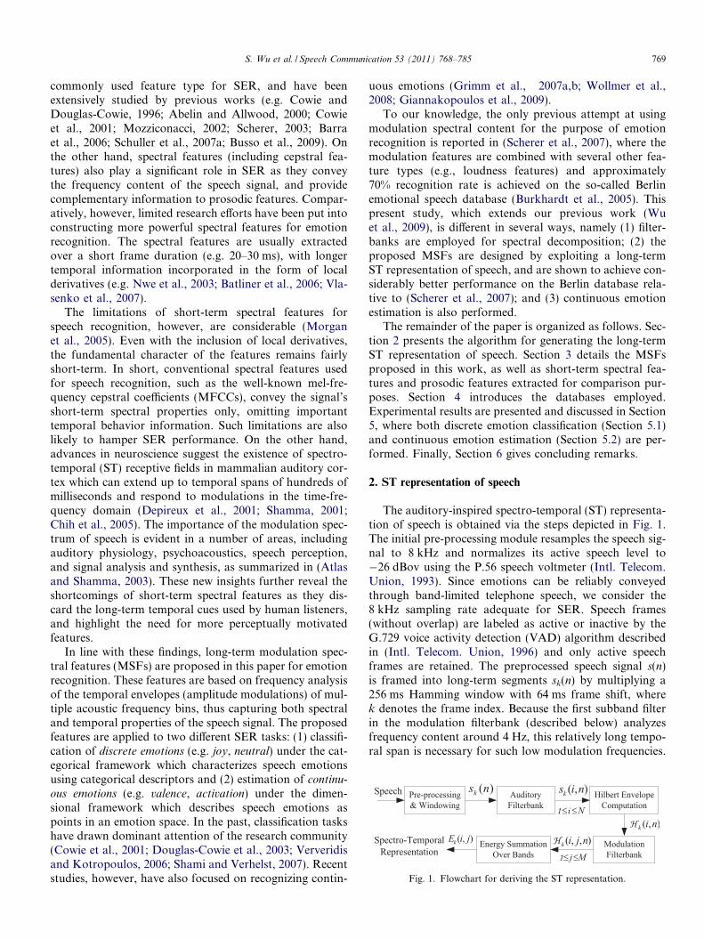
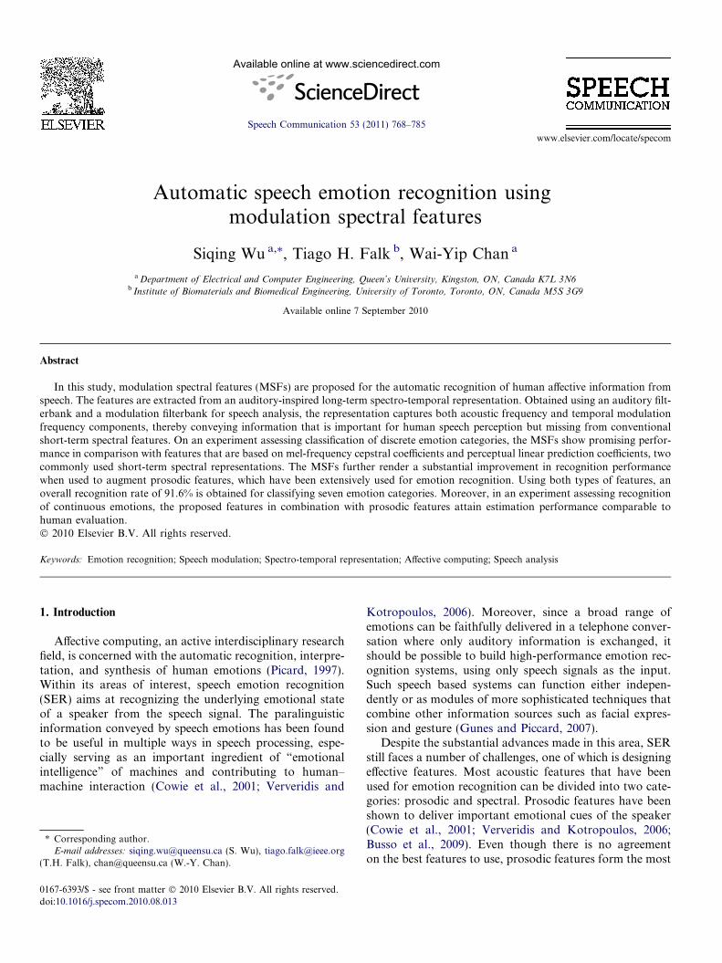
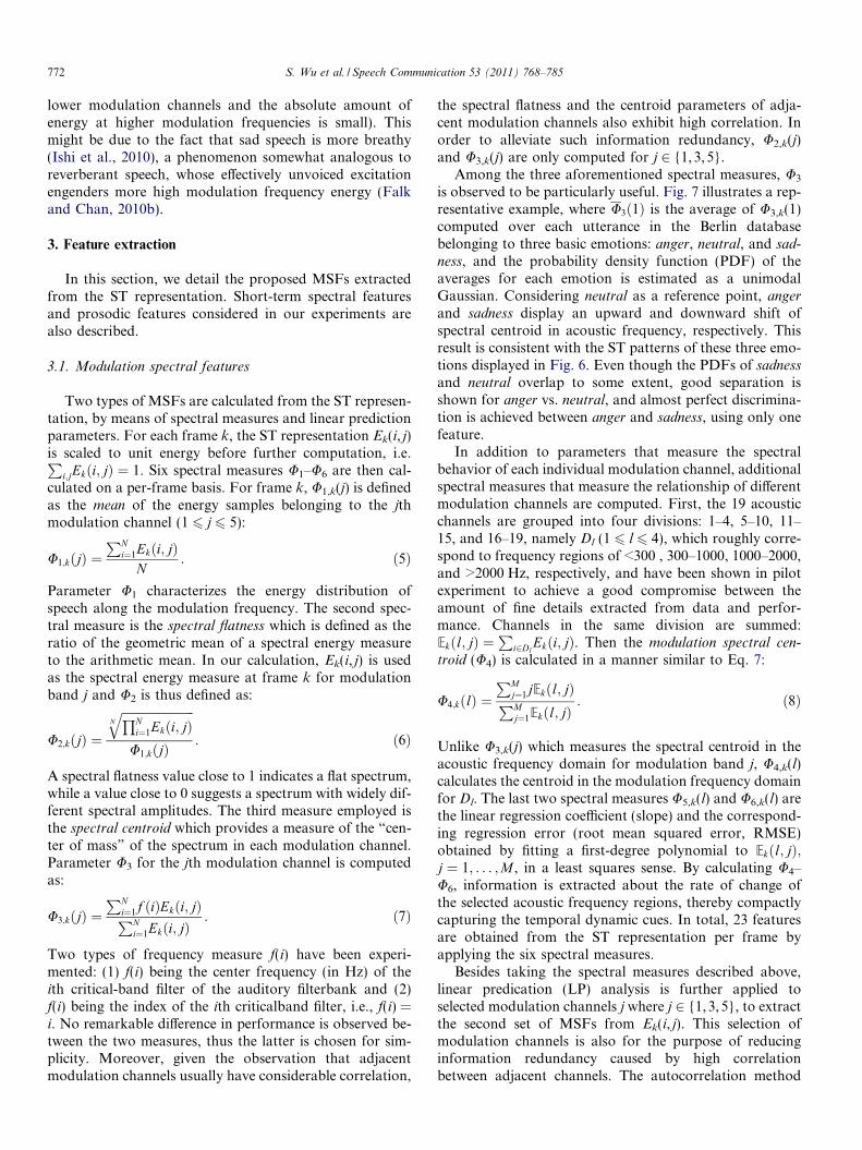
Fig. 1. Flowchart for deriving the ST representation.

S. Wu et al. / Speech Communication 53 (2011) 768–785 769

commonly used feature type for SER, and have beenextensively studied by previous works (e.g. Cowie andDouglas-Cowie, 1996; Abelin and Allwood, 2000; Cowieet al., 2001; Mozziconacci, 2002; Scherer, 2003; Barraet al., 2006; Schuller et al., 2007a; Busso et al., 2009). Onthe other hand, spectral features (including cepstral fea-tures) also play a significant role in SER as they conveythe frequency content of the speech signal, and providecomplementary information to prosodic features. Compar-atively, however, limited research efforts have been put intoconstructing more powerful spectral features for emotionrecognition. The spectral features are usually extractedover a short frame duration (e.g. 20–30 ms), with longertemporal information incorporated in the form of localderivatives (e.g. Nwe et al., 2003; Batliner et al., 2006; Vla-senko et al., 2007).

The limitations of short-term spectral features forspeech recognition, however, are considerable (Morganet al., 2005). Even with the inclusion of local derivatives,the fundamental character of the features remains fairlyshort-term. In short, conventional spectral features usedfor speech recognition, such as the well-known mel-fre-quency cepstral coefficients (MFCCs), convey the signal’sshort-term spectral properties only, omitting importanttemporal behavior information. Such limitations are alsolikely to hamper SER performance. On the other hand,advances in neuroscience suggest the existence of spectro-temporal (ST) receptive fields in mammalian auditory cor-tex which can extend up to temporal spans of hundreds ofmilliseconds and respond to modulations in the time-fre-quency domain (Depireux et al., 2001; Shamma, 2001;Chih et al., 2005). The importance of the modulation spec-trum of speech is evident in a number of areas, includingauditory physiology, psychoacoustics, speech perception,and signal analysis and synthesis, as summarized in (Atlasand Shamma, 2003). These new insights further reveal theshortcomings of short-term spectral features as they dis-card the long-term temporal cues used by human listeners,and highlight the need for more perceptually motivatedfeatures.

In line with these findings, long-term modulation spec-tral features (MSFs) are proposed in this paper for emotionrecognition. These features are based on frequency analysisof the temporal envelopes (amplitude modulations) of mul-tiple acoustic frequency bins, thus capturing both spectraland temporal properties of the speech signal. The proposedfeatures are applied to two different SER tasks: (1) classifi-cation of discrete emotions (e.g. joy, neutral) under the cat-egorical framework which characterizes speech emotionsusing categorical descriptors and (2) estimation of continu-

ous emotions (e.g. valence, activation) under the dimen-sional framework which describes speech emotions aspoints in an emotion space. In the past, classification taskshave drawn dominant attention of the research community(Cowie et al., 2001; Douglas-Cowie et al., 2003; Ververidisand Kotropoulos, 2006; Shami and Verhelst, 2007). Recentstudies, however, have also focused on recognizing contin-

uous emotions (Grimm et al., 2007a,b; Wollmer et al.,2008; Giannakopoulos et al., 2009).

To our knowledge, the only previous attempt at usingmodulation spectral content for the purpose of emotionrecognition is reported in (Scherer et al., 2007), where themodulation features are combined with several other fea-ture types (e.g., loudness features) and approximately70% recognition rate is achieved on the so-called Berlinemotional speech database (Burkhardt et al., 2005). Thispresent study, which extends our previous work (Wuet al., 2009), is different in several ways, namely (1) filter-banks are employed for spectral decomposition; (2) theproposed MSFs are designed by exploiting a long-termST representation of speech, and are shown to achieve con-siderably better performance on the Berlin database rela-tive to (Scherer et al., 2007); and (3) continuous emotionestimation is also performed.

The remainder of the paper is organized as follows. Sec-tion 2 presents the algorithm for generating the long-termST representation of speech. Section 3 details the MSFsproposed in this work, as well as short-term spectral fea-tures and prosodic features extracted for comparison pur-poses. Section 4 introduces the databases employed.Experimental results are presented and discussed in Section5, where both discrete emotion classification (Section 5.1)and continuous emotion estimation (Section 5.2) are per-formed. Finally, Section 6 gives concluding remarks.

2. ST representation of speech

The auditory-inspired spectro-temporal (ST) representa-tion of speech is obtained via the steps depicted in Fig. 1.The initial pre-processing module resamples the speech sig-nal to 8 kHz and normalizes its active speech level to�26 dBov using the P.56 speech voltmeter (Intl. Telecom.Union, 1993). Since emotions can be reliably conveyedthrough band-limited telephone speech, we consider the8 kHz sampling rate adequate for SER. Speech frames(without overlap) are labeled as active or inactive by theG.729 voice activity detection (VAD) algorithm describedin (Intl. Telecom. Union, 1996) and only active speechframes are retained. The preprocessed speech signal s(n)is framed into long-term segments sk(n) by multiplying a256 ms Hamming window with 64 ms frame shift, wherek denotes the frame index. Because the first subband filterin the modulation filterbank (described below) analyzesfrequency content around 4 Hz, this relatively long tempo-ral span is necessary for such low modulation frequencies.

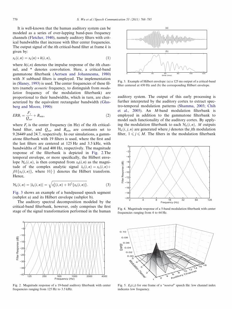
Fig. 3. Example of Hilbert envelope: (a) a 125 ms output of a critical-bandfilter centered at 650 Hz and (b) the corresponding Hilbert envelope.

Fig. 4. Magnitude response of a 5-band modulation filterbank with centerfrequencies ranging from 4 to 64 Hz.

770 S. Wu et al. / Speech Communication 53 (2011) 768–785

It is well-known that the human auditory system can bemodeled as a series of over-lapping band-pass frequencychannels (Fletcher, 1940), namely auditory filters with crit-ical bandwidths that increase with filter center frequencies.The output signal of the ith critical-band filter at frame k isgiven by:

skði; nÞ ¼ skðnÞ � hði; nÞ; ð1Þwhere h(i,n) denotes the impulse response of the ith chan-nel, and * denotes convolution. Here, a critical-bandgammatone filterbank (Aertsen and Johannesma, 1980)with N subband filters is employed. The implementationin (Slaney, 1993) is used. The center frequencies of these fil-ters (namely acoustic frequency, to distinguish from modu-

lation frequency of the modulation filterbank) areproportional to their bandwidths, which in turn, are char-acterized by the equivalent rectangular bandwidth (Glas-berg and Moore, 1990):

ERBi ¼F i

Qear

þ Bmin; ð2Þ

where Fi is the center frequency (in Hz) of the ith critical-band filter, and Qear and Bmin are constants set to9.26449 and 24.7, respectively. In our simulations, a gamm-atone filterbank with 19 filters is used, where the first andthe last filters are centered at 125 Hz and 3.5 kHz, withbandwidths of 38 and 400 Hz, respectively. The magnituderesponse of the filterbank is depicted in Fig. 2.Thetemporal envelope, or more specifically, the Hilbert enve-lope Hkði; nÞ, is then computed from sk(i,n) as the magni-tude of the complex analytic signal skði; nÞ ¼ skði; nÞþjHfskði; nÞg, where Hf�g denotes the Hilbert transform.Hence,

Hkði; nÞ ¼ jskði; nÞj ¼ffiffiffiffiffiffiffiffiffiffiffiffiffiffiffiffiffiffiffiffiffiffiffiffiffiffiffiffiffiffiffiffiffiffiffiffiffiffiffiffiffiffiffis2

kði; nÞ þH2fskði; nÞgq

: ð3Þ

Fig. 3 shows an example of a bandpassed speech segment(subplot a) and its Hilbert envelope (subplot b).

The auditory spectral decomposition modeled by thecritical-band filterbank, however, only comprises the firststage of the signal transformation performed in the human

Fig. 2. Magnitude response of a 19-band auditory filterbank with centerfrequencies ranging from 125 Hz to 3.5 kHz.

auditory system. The output of this early processing isfurther interpreted by the auditory cortex to extract spec-tro-temporal modulation patterns (Shamma, 2003; Chihet al., 2005). An M-band modulation filterbank isemployed in addition to the gammatone filterbank tomodel such functionality of the auditory cortex. By apply-ing the modulation filterbank to each Hkði; nÞ; M outputsHkði; j; nÞ are generated where j denotes the jth modulationfilter, 1 6 j 6M. The filters in the modulation filterbank

Fig. 5. Ek(i, j) for one frame of a “neutral” speech file: low channel indexindicates low frequency.

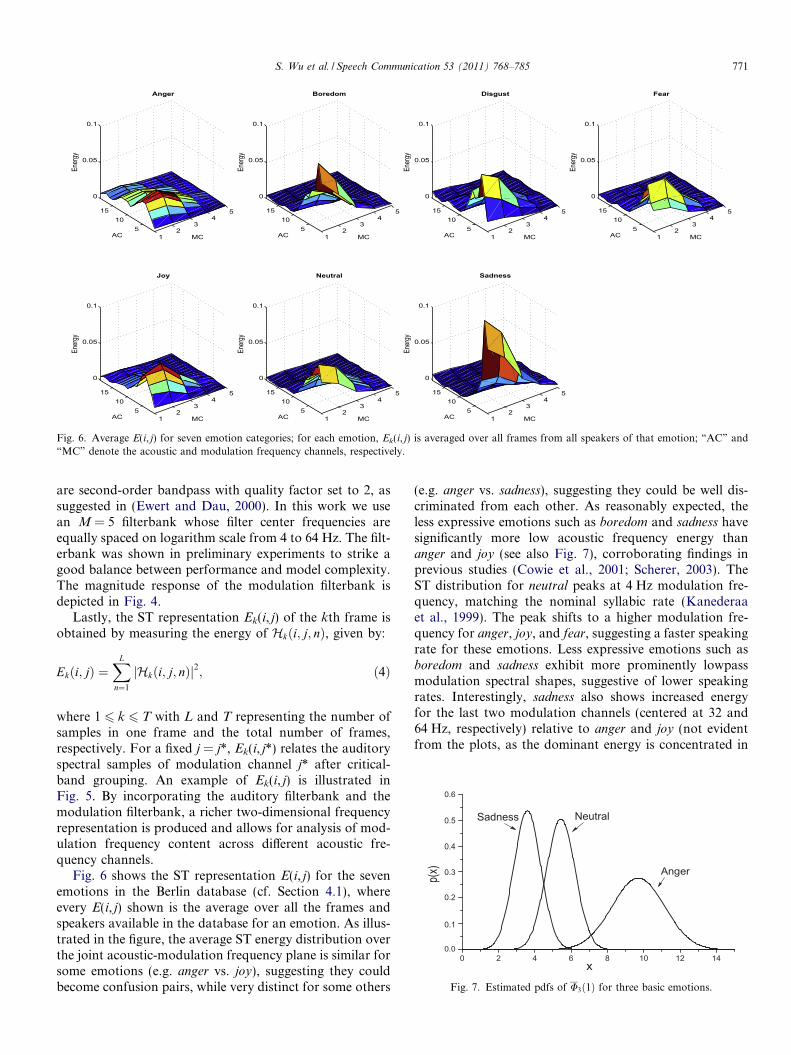
Fig. 6. Average E(i, j) for seven emotion categories; for each emotion, Ek(i, j) is averaged over all frames from all speakers of that emotion; “AC” and“MC” denote the acoustic and modulation frequency channels, respectively.

Fig. 7. Estimated pdfs of U3ð1Þ for three basic emotions.


are second-order bandpass with quality factor set to 2, assuggested in (Ewert and Dau, 2000). In this work we usean M = 5 filterbank whose filter center frequencies areequally spaced on logarithm scale from 4 to 64 Hz. The filt-erbank was shown in preliminary experiments to strike agood balance between performance and model complexity.The magnitude response of the modulation filterbank isdepicted in Fig. 4.

Lastly, the ST representation Ek(i, j) of the kth frame isobtained by measuring the energy of Hkði; j; nÞ, given by:

Ekði; jÞ ¼XL

n¼1

jHkði; j; nÞj2; ð4Þ

where 1 6 k 6 T with L and T representing the number ofsamples in one frame and the total number of frames,respectively. For a fixed j = j*, Ek(i, j*) relates the auditoryspectral samples of modulation channel j* after critical-band grouping. An example of Ek(i, j) is illustrated inFig. 5. By incorporating the auditory filterbank and themodulation filterbank, a richer two-dimensional frequencyrepresentation is produced and allows for analysis of mod-ulation frequency content across different acoustic fre-quency channels.

Fig. 6 shows the ST representation E(i, j) for the sevenemotions in the Berlin database (cf. Section 4.1), whereevery E(i, j) shown is the average over all the frames andspeakers available in the database for an emotion. As illus-trated in the figure, the average ST energy distribution overthe joint acoustic-modulation frequency plane is similar forsome emotions (e.g. anger vs. joy), suggesting they couldbecome confusion pairs, while very distinct for some others

(e.g. anger vs. sadness), suggesting they could be well dis-criminated from each other. As reasonably expected, theless expressive emotions such as boredom and sadness havesignificantly more low acoustic frequency energy thananger and joy (see also Fig. 7), corroborating findings inprevious studies (Cowie et al., 2001; Scherer, 2003). TheST distribution for neutral peaks at 4 Hz modulation fre-quency, matching the nominal syllabic rate (Kanederaaet al., 1999). The peak shifts to a higher modulation fre-quency for anger, joy, and fear, suggesting a faster speakingrate for these emotions. Less expressive emotions such asboredom and sadness exhibit more prominently lowpassmodulation spectral shapes, suggestive of lower speakingrates. Interestingly, sadness also shows increased energyfor the last two modulation channels (centered at 32 and64 Hz, respectively) relative to anger and joy (not evidentfrom the plots, as the dominant energy is concentrated in


lower modulation channels and the absolute amount ofenergy at higher modulation frequencies is small). Thismight be due to the fact that sad speech is more breathy(Ishi et al., 2010), a phenomenon somewhat analogous toreverberant speech, whose effectively unvoiced excitationengenders more high modulation frequency energy (Falkand Chan, 2010b).

3. Feature extraction

In this section, we detail the proposed MSFs extractedfrom the ST representation. Short-term spectral featuresand prosodic features considered in our experiments arealso described.

3.1. Modulation spectral features

Two types of MSFs are calculated from the ST represen-tation, by means of spectral measures and linear predictionparameters. For each frame k, the ST representation Ek(i, j)is scaled to unit energy before further computation, i.e.P

i;jEkði; jÞ ¼ 1. Six spectral measures U1–U6 are then cal-culated on a per-frame basis. For frame k, U1,k(j) is definedas the mean of the energy samples belonging to the jthmodulation channel (1 6 j 6 5):

U1;kðjÞ ¼PN

i¼1Ekði; jÞN

: ð5Þ

Parameter U1 characterizes the energy distribution ofspeech along the modulation frequency. The second spec-tral measure is the spectral flatness which is defined as theratio of the geometric mean of a spectral energy measureto the arithmetic mean. In our calculation, Ek(i, j) is usedas the spectral energy measure at frame k for modulationband j and U2 is thus defined as:

U2;kðjÞ ¼

ffiffiffiffiffiffiffiffiffiffiffiffiffiffiffiffiffiffiffiffiffiffiffiffiQNi¼1Ekði; jÞN

q

U1;kðjÞ: ð6Þ

A spectral flatness value close to 1 indicates a flat spectrum,while a value close to 0 suggests a spectrum with widely dif-ferent spectral amplitudes. The third measure employed isthe spectral centroid which provides a measure of the “cen-ter of mass” of the spectrum in each modulation channel.Parameter U3 for the jth modulation channel is computedas:

U3;kðjÞ ¼PN

i¼1f ðiÞEkði; jÞPNi¼1Ekði; jÞ

: ð7Þ

Two types of frequency measure f(i) have been experi-mented: (1) f(i) being the center frequency (in Hz) of theith critical-band filter of the auditory filterbank and (2)f(i) being the index of the ith criticalband filter, i.e., f(i) =i. No remarkable difference in performance is observed be-tween the two measures, thus the latter is chosen for sim-plicity. Moreover, given the observation that adjacentmodulation channels usually have considerable correlation,

the spectral flatness and the centroid parameters of adja-cent modulation channels also exhibit high correlation. Inorder to alleviate such information redundancy, U2,k(j)and U3,k(j) are only computed for j 2 {1,3,5}.

Among the three aforementioned spectral measures, U3

is observed to be particularly useful. Fig. 7 illustrates a rep-resentative example, where U3ð1Þ is the average of U3,k(1)computed over each utterance in the Berlin databasebelonging to three basic emotions: anger, neutral, and sad-

ness, and the probability density function (PDF) of theaverages for each emotion is estimated as a unimodalGaussian. Considering neutral as a reference point, anger

and sadness display an upward and downward shift ofspectral centroid in acoustic frequency, respectively. Thisresult is consistent with the ST patterns of these three emo-tions displayed in Fig. 6. Even though the PDFs of sadness

and neutral overlap to some extent, good separation isshown for anger vs. neutral, and almost perfect discrimina-tion is achieved between anger and sadness, using only onefeature.

In addition to parameters that measure the spectralbehavior of each individual modulation channel, additionalspectral measures that measure the relationship of differentmodulation channels are computed. First, the 19 acousticchannels are grouped into four divisions: 1–4, 5–10, 11–15, and 16–19, namely Dl (1 6 l 6 4), which roughly corre-spond to frequency regions of <300 , 300–1000, 1000–2000,and >2000 Hz, respectively, and have been shown in pilotexperiment to achieve a good compromise between theamount of fine details extracted from data and perfor-mance. Channels in the same division are summed:Ekðl; jÞ ¼

Pi2Dl

Ekði; jÞ. Then the modulation spectral cen-

troid (U4) is calculated in a manner similar to Eq. 7:

U4;kðlÞ ¼PM

j¼1jEkðl; jÞPMj¼1Ekðl; jÞ

: ð8Þ

Unlike U3,k(j) which measures the spectral centroid in theacoustic frequency domain for modulation band j, U4,k(l)calculates the centroid in the modulation frequency domainfor Dl. The last two spectral measures U5,k(l) and U6,k(l) arethe linear regression coefficient (slope) and the correspond-ing regression error (root mean squared error, RMSE)obtained by fitting a first-degree polynomial to Ekðl; jÞ;j ¼ 1; . . . ;M , in a least squares sense. By calculating U4–U6, information is extracted about the rate of change ofthe selected acoustic frequency regions, thereby compactlycapturing the temporal dynamic cues. In total, 23 featuresare obtained from the ST representation per frame byapplying the six spectral measures.

Besides taking the spectral measures described above,linear predication (LP) analysis is further applied toselected modulation channels j where j 2 {1,3,5}, to extractthe second set of MSFs from Ek(i, j). This selection ofmodulation channels is also for the purpose of reducinginformation redundancy caused by high correlationbetween adjacent channels. The autocorrelation method

Table 1List of prosodic features.

Pitch, intensity, delta-pitch, delta-intensity

Mean, std. dev., skewness, kurtosis, shimmer, maximum, minimum,median, quartiles, range, differences between quartiles, linear & quadraticregression coefficients, regression error (RMSE)

Speaking rate

Mean and std. dev. of syllable durations, ratio between the duration ofvoiced and unvoiced speech

Others

Zero-crossing rate (ZCR), Teager energy operator (TEO)


for autoregressive (AR) modeling is used here. In orderto suppress local details while preserving the broad struc-ture beneficial to recognition, a 5th-order all-pole modelis used to approximate the spectral samples. The compu-tational cost of this AR modeling is negligible due to thelow LP order and the small number of spectral samplesper modulation channel (19 here). The LP coefficientsobtained are further transformed into cepstral coefficients(LPCCs), and denoted as Ck(n, j) (0 6 n 6 5). The LPCCshave been shown to be generally more robust and reliablefor speech recognition than the direct LP coefficients(Rabiner and Juang, 1993). We have tested both typesand indeed the LPCCs yield better recognition perfor-mance in our application. Together with the 23 aforemen-tioned features, a total of 41 MSFs are calculated frame-by-frame.

Although MSFs are extracted at a frame-level (FL),the common approach in current SER literature com-putes features at the utterance-level (UL) (e.g. Grimmet al., 2007a,b; Shami and Verhelst, 2007; Schulleret al., 2007b; Clavel et al., 2008; Lugger and Yang,2008; Busso et al., 2009; Giannakopoulos et al., 2009;Sun and Torres, 2009), by applying descriptive functions(typically statistical) to the trajectories of FL features(and often also their derivatives to convey local dynamicinformation). The UL features capture the global proper-ties and behaviors of their FL counterparts. It is desirablefor the UL features to capture the supra-segmental char-acteristics of emotional speech that can be attributed toemotions rather than specific spoken-content and to effec-tively avoid problems such as spoken-content over-model-ing (Vlasenko et al., 2007). Following the UL approach,two basic statistics: mean and standard deviation (std.dev.) of the FL MSFs are calculated in this work, pro-ducing 82 UL MSFs.

3.2. Short-term spectral features

3.2.1. MFCC featuresThe mel-frequency cepstral coefficients (MFCCs), first

introduced in (Davis and Mermelstein, 1980) and success-fully applied to automatic speech recognition, are popularshort-term spectral features used for emotion recognition.They are extracted here for comparison with the proposedlong-term MSFs. The speech signal is first filtered by ahigh-pass filter with a pre-emphasis coefficient of 0.97,and the first 13 MFCCs (including the zeroth order log-energy coefficient) are extracted from 25 ms Hamming-win-dowed speech frames every 10 ms. As a common practice,the delta and double-delta MFCCs describing local dynam-ics are calculated as well to form a 39-dimensional FL fea-ture vector. The most frequently used UL MFCC featuresfor emotion recognition include mean and std. dev. (or var-iance) of the first 13 MFCCs and their deltas (e.g. Grimmet al., 2007a,b; Schuller et al., 2007a; Vlasenko et al., 2007;Clavel et al., 2008; Lugger and Yang, 2008). In this work,we compute mean, std. dev., and 3rd–5th central moments

of the first 13 MFCCs, as well as their deltas and double-deltas, giving 195 MFCC features in total. This MFCCfeature set is an extension to the one used in (Grimmet al., 2007a, 2008), by further considering the deltacoefficients.

3.2.2. PLP features

In addition to MFCCs, perceptual linear predictive(PLP) coefficients (Hermansky, 1990) are also extractedfrom speech, serving as an alternative choice of short-termspectral features for comparison. PLP analysis approxi-mates the auditory spectrum of speech by an all-pole modelthat is more consistent with human hearing than conven-tional linear predictive analysis. A 5th-order model isemployed as suggested in (Hermansky, 1990). The PLPcoefficients are transformed to cepstral coefficients c(n)(0 6 n 6 5). The delta and double-delta coefficients are alsoconsidered. The aforementioned statistical parameters asused for MFCC are calculated for the PLP coefficients, giv-ing 90 candidate PLP features.

3.3. Prosodic features

Prosodic features have been, among numerous acousticfeatures employed for SER, the most widely used featuretype as mentioned in Section 1. Hence they are used hereas a benchmark, and more importantly, to verify whetherthe MSFs can serve as useful additions to the extensivelyused prosodic features. The most commonly used prosodicfeatures are based on pitch, intensity, and speaking rate.The features are estimated on a short-term frame basis,and their contours are used to compute UL features. Thestatistics of these trajectories are shown to be of fundamen-tal importance for conveying emotional cues (Cowie et al.,2001; Nwe et al., 2003; Ververidis and Kotropoulos, 2006;Busso et al., 2009).

In total, 75 prosodic features are extracted as listed inTable 1. Note that a complete coverage of prosodic fea-tures is infeasible. Consequently, the features calculatedhere are by no means exhaustive, but serve as a representa-tive sampling of the essential prosodic feature space. Pitchis computed for voiced speech using the pitch trackingalgorithm in (Talkin, 1995), and intensity is measured for

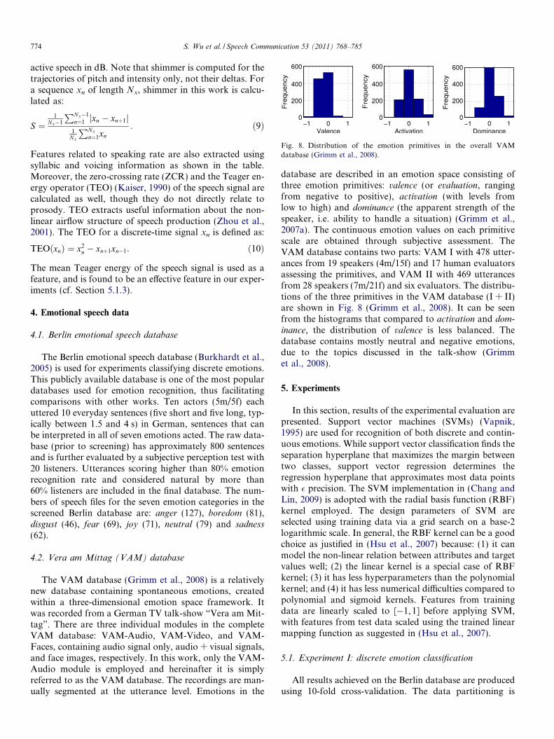
Fig. 8. Distribution of the emotion primitives in the overall VAMdatabase (Grimm et al., 2008).


active speech in dB. Note that shimmer is computed for thetrajectories of pitch and intensity only, not their deltas. Fora sequence xn of length Nx, shimmer in this work is calcu-lated as:

S ¼1

Nx�1

PNx�1n¼1 jxn � xnþ1j

1Nx

PNxn¼1xn

: ð9Þ

Features related to speaking rate are also extracted usingsyllabic and voicing information as shown in the table.Moreover, the zero-crossing rate (ZCR) and the Teager en-ergy operator (TEO) (Kaiser, 1990) of the speech signal arecalculated as well, though they do not directly relate toprosody. TEO extracts useful information about the non-linear airflow structure of speech production (Zhou et al.,2001). The TEO for a discrete-time signal xn is defined as:

TEOðxnÞ ¼ x2n � xnþ1xn�1: ð10Þ

The mean Teager energy of the speech signal is used as afeature, and is found to be an effective feature in our exper-iments (cf. Section 5.1.3).

4. Emotional speech data

4.1. Berlin emotional speech database

The Berlin emotional speech database (Burkhardt et al.,2005) is used for experiments classifying discrete emotions.This publicly available database is one of the most populardatabases used for emotion recognition, thus facilitatingcomparisons with other works. Ten actors (5m/5f) eachuttered 10 everyday sentences (five short and five long, typ-ically between 1.5 and 4 s) in German, sentences that canbe interpreted in all of seven emotions acted. The raw data-base (prior to screening) has approximately 800 sentencesand is further evaluated by a subjective perception test with20 listeners. Utterances scoring higher than 80% emotionrecognition rate and considered natural by more than60% listeners are included in the final database. The num-bers of speech files for the seven emotion categories in thescreened Berlin database are: anger (127), boredom (81),disgust (46), fear (69), joy (71), neutral (79) and sadness

(62).

4.2. Vera am Mittag (VAM) database

The VAM database (Grimm et al., 2008) is a relativelynew database containing spontaneous emotions, createdwithin a three-dimensional emotion space framework. Itwas recorded from a German TV talk-show “Vera am Mit-tag”. There are three individual modules in the completeVAM database: VAM-Audio, VAM-Video, and VAM-Faces, containing audio signal only, audio + visual signals,and face images, respectively. In this work, only the VAM-Audio module is employed and hereinafter it is simplyreferred to as the VAM database. The recordings are man-ually segmented at the utterance level. Emotions in the

database are described in an emotion space consisting ofthree emotion primitives: valence (or evaluation, rangingfrom negative to positive), activation (with levels fromlow to high) and dominance (the apparent strength of thespeaker, i.e. ability to handle a situation) (Grimm et al.,2007a). The continuous emotion values on each primitivescale are obtained through subjective assessment. TheVAM database contains two parts: VAM I with 478 utter-ances from 19 speakers (4m/15f) and 17 human evaluatorsassessing the primitives, and VAM II with 469 utterancesfrom 28 speakers (7m/21f) and six evaluators. The distribu-tions of the three primitives in the VAM database (I + II)are shown in Fig. 8 (Grimm et al., 2008). It can be seenfrom the histograms that compared to activation and dom-

inance, the distribution of valence is less balanced. Thedatabase contains mostly neutral and negative emotions,due to the topics discussed in the talk-show (Grimmet al., 2008).

5. Experiments

In this section, results of the experimental evaluation arepresented. Support vector machines (SVMs) (Vapnik,1995) are used for recognition of both discrete and contin-uous emotions. While support vector classification finds theseparation hyperplane that maximizes the margin betweentwo classes, support vector regression determines theregression hyperplane that approximates most data pointswith � precision. The SVM implementation in (Chang andLin, 2009) is adopted with the radial basis function (RBF)kernel employed. The design parameters of SVM areselected using training data via a grid search on a base-2logarithmic scale. In general, the RBF kernel can be a goodchoice as justified in (Hsu et al., 2007) because: (1) it canmodel the non-linear relation between attributes and targetvalues well; (2) the linear kernel is a special case of RBFkernel; (3) it has less hyperparameters than the polynomialkernel; and (4) it has less numerical difficulties compared topolynomial and sigmoid kernels. Features from trainingdata are linearly scaled to [�1,1] before applying SVM,with features from test data scaled using the trained linearmapping function as suggested in (Hsu et al., 2007).

5.1. Experiment I: discrete emotion classification

All results achieved on the Berlin database are producedusing 10-fold cross-validation. The data partitioning is

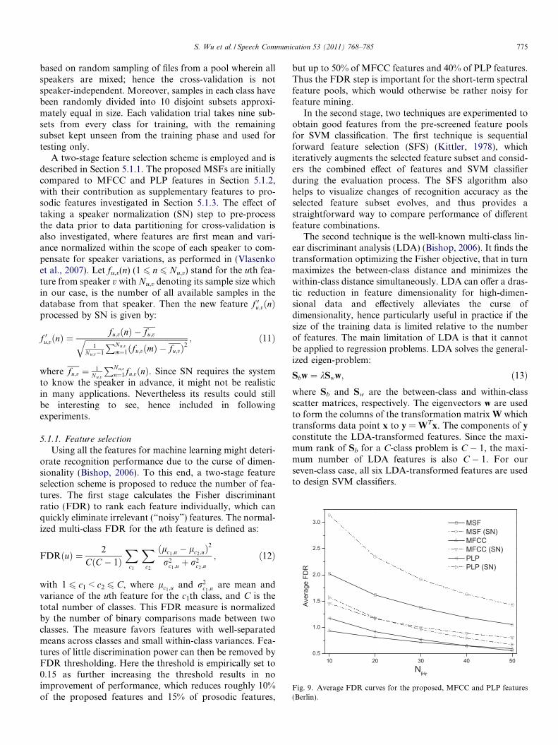
Fig. 9. Average FDR curves for the proposed, MFCC and PLP features(Berlin).


based on random sampling of files from a pool wherein allspeakers are mixed; hence the cross-validation is notspeaker-independent. Moreover, samples in each class havebeen randomly divided into 10 disjoint subsets approxi-mately equal in size. Each validation trial takes nine sub-sets from every class for training, with the remainingsubset kept unseen from the training phase and used fortesting only.

A two-stage feature selection scheme is employed and isdescribed in Section 5.1.1. The proposed MSFs are initiallycompared to MFCC and PLP features in Section 5.1.2,with their contribution as supplementary features to pro-sodic features investigated in Section 5.1.3. The effect oftaking a speaker normalization (SN) step to pre-processthe data prior to data partitioning for cross-validation isalso investigated, where features are first mean and vari-ance normalized within the scope of each speaker to com-pensate for speaker variations, as performed in (Vlasenkoet al., 2007). Let fu,v(n) (1 6 n 6 Nu,v) stand for the uth fea-ture from speaker v with Nu,v denoting its sample size whichin our case, is the number of all available samples in thedatabase from that speaker. Then the new feature f 0u;vðnÞprocessed by SN is given by:

f 0u;vðnÞ ¼fu;vðnÞ � fu;vffiffiffiffiffiffiffiffiffiffiffiffiffiffiffiffiffiffiffiffiffiffiffiffiffiffiffiffiffiffiffiffiffiffiffiffiffiffiffiffiffiffiffiffiffiffiffiffiffiffiffiffiffi

1Nu;v�1

PNu;vm¼1ðfu;vðmÞ � fu;vÞ2

q ; ð11Þ

where fu;v ¼ 1Nu;v

PNu;v

n¼1fu;vðnÞ. Since SN requires the systemto know the speaker in advance, it might not be realisticin many applications. Nevertheless its results could stillbe interesting to see, hence included in followingexperiments.

5.1.1. Feature selection

Using all the features for machine learning might deteri-orate recognition performance due to the curse of dimen-sionality (Bishop, 2006). To this end, a two-stage featureselection scheme is proposed to reduce the number of fea-tures. The first stage calculates the Fisher discriminantratio (FDR) to rank each feature individually, which canquickly eliminate irrelevant (“noisy”) features. The normal-ized multi-class FDR for the uth feature is defined as:

FDRðuÞ ¼ 2

CðC � 1ÞX

c1

Xc2

ðlc1;u � lc2;uÞ2

r2c1;uþ r2

c2;u

; ð12Þ

with 1 6 c1 < c2 6 C, where lc1;u and r2c1;u

are mean andvariance of the uth feature for the c1th class, and C is thetotal number of classes. This FDR measure is normalizedby the number of binary comparisons made between twoclasses. The measure favors features with well-separatedmeans across classes and small within-class variances. Fea-tures of little discrimination power can then be removed byFDR thresholding. Here the threshold is empirically set to0.15 as further increasing the threshold results in noimprovement of performance, which reduces roughly 10%of the proposed features and 15% of prosodic features,

but up to 50% of MFCC features and 40% of PLP features.Thus the FDR step is important for the short-term spectralfeature pools, which would otherwise be rather noisy forfeature mining.

In the second stage, two techniques are experimented toobtain good features from the pre-screened feature poolsfor SVM classification. The first technique is sequentialforward feature selection (SFS) (Kittler, 1978), whichiteratively augments the selected feature subset and consid-ers the combined effect of features and SVM classifierduring the evaluation process. The SFS algorithm alsohelps to visualize changes of recognition accuracy as theselected feature subset evolves, and thus provides astraightforward way to compare performance of differentfeature combinations.

The second technique is the well-known multi-class lin-ear discriminant analysis (LDA) (Bishop, 2006). It finds thetransformation optimizing the Fisher objective, that in turnmaximizes the between-class distance and minimizes thewithin-class distance simultaneously. LDA can offer a dras-tic reduction in feature dimensionality for high-dimen-sional data and effectively alleviates the curse ofdimensionality, hence particularly useful in practice if thesize of the training data is limited relative to the numberof features. The main limitation of LDA is that it cannotbe applied to regression problems. LDA solves the general-ized eigen-problem:

Sbw ¼ kSww; ð13Þwhere Sb and Sw are the between-class and within-classscatter matrices, respectively. The eigenvectors w are usedto form the columns of the transformation matrix W whichtransforms data point x to y = WTx. The components of y

constitute the LDA-transformed features. Since the maxi-mum rank of Sb for a C-class problem is C � 1, the maxi-mum number of LDA features is also C � 1. For ourseven-class case, all six LDA-transformed features are usedto design SVM classifiers.

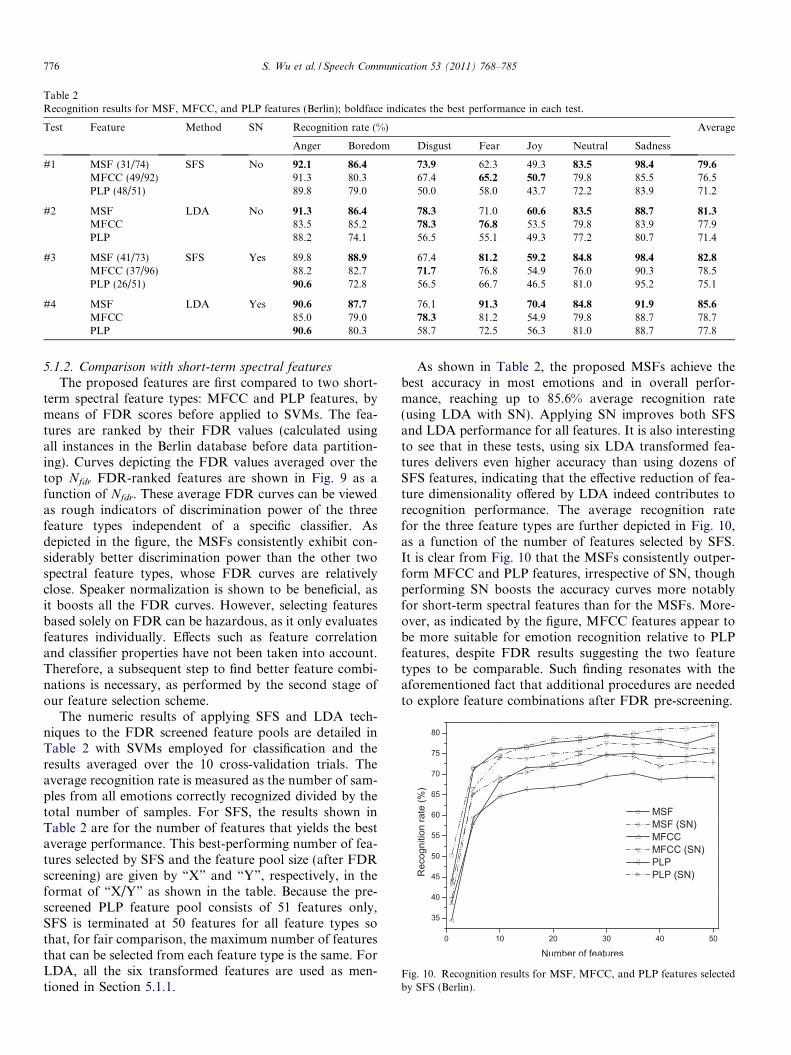
Table 2Recognition results for MSF, MFCC, and PLP features (Berlin); boldface indicates the best performance in each test.

Test Feature Method SN Recognition rate (%) Average

Anger Boredom Disgust Fear Joy Neutral Sadness

#1 MSF (31/74) SFS No 92.1 86.4 73.9 62.3 49.3 83.5 98.4 79.6

MFCC (49/92) 91.3 80.3 67.4 65.2 50.7 79.8 85.5 76.5PLP (48/51) 89.8 79.0 50.0 58.0 43.7 72.2 83.9 71.2

#2 MSF LDA No 91.3 86.4 78.3 71.0 60.6 83.5 88.7 81.3

MFCC 83.5 85.2 78.3 76.8 53.5 79.8 83.9 77.9PLP 88.2 74.1 56.5 55.1 49.3 77.2 80.7 71.4

#3 MSF (41/73) SFS Yes 89.8 88.9 67.4 81.2 59.2 84.8 98.4 82.8

MFCC (37/96) 88.2 82.7 71.7 76.8 54.9 76.0 90.3 78.5PLP (26/51) 90.6 72.8 56.5 66.7 46.5 81.0 95.2 75.1

#4 MSF LDA Yes 90.6 87.7 76.1 91.3 70.4 84.8 91.9 85.6

MFCC 85.0 79.0 78.3 81.2 54.9 79.8 88.7 78.7PLP 90.6 80.3 58.7 72.5 56.3 81.0 88.7 77.8

Fig. 10. Recognition results for MSF, MFCC, and PLP features selectedby SFS (Berlin).


5.1.2. Comparison with short-term spectral features

The proposed features are first compared to two short-term spectral feature types: MFCC and PLP features, bymeans of FDR scores before applied to SVMs. The fea-tures are ranked by their FDR values (calculated usingall instances in the Berlin database before data partition-ing). Curves depicting the FDR values averaged over thetop Nfdr FDR-ranked features are shown in Fig. 9 as afunction of Nfdr. These average FDR curves can be viewedas rough indicators of discrimination power of the threefeature types independent of a specific classifier. Asdepicted in the figure, the MSFs consistently exhibit con-siderably better discrimination power than the other twospectral feature types, whose FDR curves are relativelyclose. Speaker normalization is shown to be beneficial, asit boosts all the FDR curves. However, selecting featuresbased solely on FDR can be hazardous, as it only evaluatesfeatures individually. Effects such as feature correlationand classifier properties have not been taken into account.Therefore, a subsequent step to find better feature combi-nations is necessary, as performed by the second stage ofour feature selection scheme.

The numeric results of applying SFS and LDA tech-niques to the FDR screened feature pools are detailed inTable 2 with SVMs employed for classification and theresults averaged over the 10 cross-validation trials. Theaverage recognition rate is measured as the number of sam-ples from all emotions correctly recognized divided by thetotal number of samples. For SFS, the results shown inTable 2 are for the number of features that yields the bestaverage performance. This best-performing number of fea-tures selected by SFS and the feature pool size (after FDRscreening) are given by “X” and “Y”, respectively, in theformat of “X/Y” as shown in the table. Because the pre-screened PLP feature pool consists of 51 features only,SFS is terminated at 50 features for all feature types sothat, for fair comparison, the maximum number of featuresthat can be selected from each feature type is the same. ForLDA, all the six transformed features are used as men-tioned in Section 5.1.1.

As shown in Table 2, the proposed MSFs achieve thebest accuracy in most emotions and in overall perfor-mance, reaching up to 85.6% average recognition rate(using LDA with SN). Applying SN improves both SFSand LDA performance for all features. It is also interestingto see that in these tests, using six LDA transformed fea-tures delivers even higher accuracy than using dozens ofSFS features, indicating that the effective reduction of fea-ture dimensionality offered by LDA indeed contributes torecognition performance. The average recognition ratefor the three feature types are further depicted in Fig. 10,as a function of the number of features selected by SFS.It is clear from Fig. 10 that the MSFs consistently outper-form MFCC and PLP features, irrespective of SN, thoughperforming SN boosts the accuracy curves more notablyfor short-term spectral features than for the MSFs. More-over, as indicated by the figure, MFCC features appear tobe more suitable for emotion recognition relative to PLPfeatures, despite FDR results suggesting the two featuretypes to be comparable. Such finding resonates with theaforementioned fact that additional procedures are neededto explore feature combinations after FDR pre-screening.

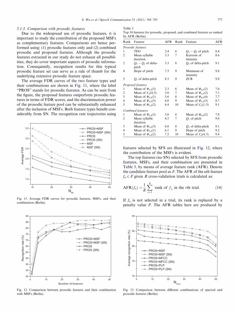
Table 3Top 10 features for prosodic, proposed, and combined features as rankedby AFR (Berlin).

Rank Feature AFR Rank Feature AFR

Prosodic features

1 TEO 2.4 6 Q3 � Q2 of pitch 8.42 Mean syllable

duration3.3 7 Kurtosis of

intensity8.6

2 Q3 � Q2 of delta-pitch

3.3 8 Q3 of delta-pitch 9.1

4 Slope of pitch 7.3 9 Minimum ofintensity

9.8

5 Q1 of delta-pitch 8.3 9 ZCR 9.8

Proposed features

1 Mean of U1,k(3) 2.3 6 Mean of U6,k(2) 7.02 Mean of Ck(4,5) 5.0 7 Mean of U1,k(2) 7.13 Mean of U3,k(1) 5.6 8 Mean of U4,k(4) 7.74 Mean of U3,k(3) 6.0 9 Mean of U3,k(5) 8.75 Mean of U5,k(2) 6.4 10 Mean of Ck(1,5) 9.1

Combined features

1 Mean of U1,k(3) 3.0 6 Mean of U6,k(2) 7.8


5.1.3. Comparison with prosodic features

Due to the widespread use of prosodic features, it isimportant to study the contribution of the proposed MSFsas complementary features. Comparisons are hence per-formed using: (1) prosodic features only and (2) combinedprosodic and proposed features. Although the prosodicfeatures extracted in our study do not exhaust all possibil-ities, they do cover important aspects of prosodic informa-tion. Consequently, recognition results for this typicalprosodic feature set can serve as a rule of thumb for theunderlying extensive prosodic feature space.

The average FDR curves of the two feature types andtheir combinations are shown in Fig. 11, where the label“PROS” stands for prosodic features. As can be seen fromthe figure, the proposed features outperform prosodic fea-tures in terms of FDR scores, and the discrimination powerof the prosodic feature pool can be substantially enhancedafter the inclusion of MSFs. Both feature types benefit con-siderably from SN. The recognition rate trajectories using

Fig. 11. Average FDR curves for prosodic features, MSFs, and theircombination (Berlin).

Fig. 12. Comparison between prosodic features and their combinationwith MSFs (Berlin).

2 Mean syllableduration

4.5 7 Q1 of pitch 9.0

3 Mean of U3,k(3) 6.0 8 Q1 of delta-pitch 9.14 Mean of U3,k(1) 6.1 9 Slope of pitch 9.25 Mean of U5,k(2) 7.2 10 Mean of Ck(4,5) 9.4

features selected by SFS are illustrated in Fig. 12, wherethe contribution of the MSFs is evident.

The top features (no SN) selected by SFS from prosodicfeatures, MSFs, and their combination are presented inTable 3, by means of average feature rank (AFR). Denotethe candidate feature pool as F. The AFR of the uth featurefu 2 F given R cross-validation trials is calculated as:

AFRðfuÞ ¼1

R

XR

r¼1

rank of f u in the rth trial: ð14Þ

If fu is not selected in a trial, its rank is replaced by apenalty value P. The AFR tables here are produced by

Fig. 13. Comparison between different combinations of spectral andprosodic features (Berlin).


selecting the top 10 features in each trial with the penaltyvalue P set to 11. Features with small AFR values, suchas TEO and U1,k(3), are consistently top ranked acrossthe cross-validation trials. In practice, such results can beused to pick features when forming a final feature set totrain the classifier. We also compiled AFR tables for fea-tures with SN (not shown). It is observed that nearly halfof the features in Table 3 appear in the SN case as well,though with different ranks, and several features remaintop ranked regardless of SN, such as TEO, mean syllableduration, U1,k(3) and U3,k(1).

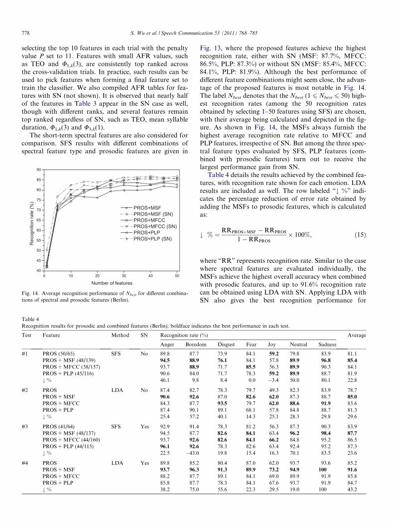
The short-term spectral features are also considered forcomparison. SFS results with different combinations ofspectral feature type and prosodic features are given in

Fig. 14. Average recognition performance of Nbest for different combina-tions of spectral and prosodic features (Berlin).

Table 4Recognition results for prosodic and combined features (Berlin); boldface ind

Test Feature Method SN Recognition rate

Anger Bored

#1 PROS (50/65) SFS No 89.8 87.7PROS + MSF (48/139) 94.5 88.9

PROS + MFCC (38/157) 93.7 88.9

PROS + PLP (45/116) 90.6 84.0# % 46.1 9.8

#2 PROS LDA No 87.4 82.7PROS + MSF 90.6 92.6

PROS + MFCC 84.3 87.7PROS + PLP 87.4 90.1# % 25.4 57.2

#3 PROS (41/64) SFS Yes 92.9 91.4PROS + MSF (48/137) 94.5 87.7PROS + MFCC (44/160) 93.7 92.6

PROS + PLP (44/115) 96.1 92.6

# % 22.5 �43.0

#4 PROS LDA Yes 89.8 85.2PROS + MSF 93.7 96.3

PROS + MFCC 88.2 87.7PROS + PLP 85.8 87.7# % 38.2 75.0

Fig. 13, where the proposed features achieve the highestrecognition rate, either with SN (MSF: 87.7%, MFCC:86.5%, PLP: 87.3%) or without SN (MSF: 85.4%, MFCC:84.1%, PLP: 81.9%). Although the best performance ofdifferent feature combinations might seem close, the advan-tage of the proposed features is most notable in Fig. 14.The label Nbest denotes that the Nbest (1 6 Nbest 6 50) high-est recognition rates (among the 50 recognition ratesobtained by selecting 1–50 features using SFS) are chosen,with their average being calculated and depicted in the fig-ure. As shown in Fig. 14, the MSFs always furnish thehighest average recognition rate relative to MFCC andPLP features, irrespective of SN. But among the three spec-tral feature types evaluated by SFS, PLP features (com-bined with prosodic features) turn out to receive thelargest performance gain from SN.

Table 4 details the results achieved by the combined fea-tures, with recognition rate shown for each emotion. LDAresults are included as well. The row labeled “# %” indi-cates the percentage reduction of error rate obtained byadding the MSFs to prosodic features, which is calculatedas:

# % ¼ RRPROSþMSF �RRPROS

1�RRPROS

� 100%; ð15Þ

where “RR” represents recognition rate. Similar to the casewhere spectral features are evaluated individually, theMSFs achieve the highest overall accuracy when combinedwith prosodic features, and up to 91.6% recognition ratecan be obtained using LDA with SN. Applying LDA withSN also gives the best recognition performance for

icates the best performance in each test.

(%) Average

om Disgust Fear Joy Neutral Sadness

73.9 84.1 59.2 79.8 83.9 81.176.1 84.1 57.8 89.9 96.8 85.4

71.7 85.5 56.3 89.9 90.3 84.171.7 78.3 59.2 89.9 88.7 81.98.4 0.0 �3.4 50.0 80.1 22.8

78.3 79.7 49.3 82.3 83.9 78.787.0 82.6 62.0 87.3 88.7 85.0

93.5 79.7 62.0 88.6 91.9 83.689.1 68.1 57.8 84.8 88.7 81.340.1 14.3 25.1 28.3 29.8 29.6

78.3 81.2 56.3 87.3 90.3 83.982.6 84.1 63.4 96.2 98.4 87.7

82.6 84.1 66.2 84.8 95.2 86.578.3 82.6 63.4 92.4 95.2 87.319.8 15.4 16.3 70.1 83.5 23.6

80.4 87.0 62.0 93.7 93.6 85.291.3 89.9 73.2 94.9 100 91.6

89.1 84.1 69.0 89.9 91.9 85.878.3 84.1 67.6 93.7 91.9 84.755.6 22.3 29.5 19.0 100 43.2

Table 5Confusion matrix for using only prosodic features (Berlin).

Emotion Anger Boredom Disgust Fear Joy Neutral Sadness Rate (%)

Anger 114 0 1 3 8 1 0 89.8Boredom 0 69 1 0 0 8 3 85.2Disgust 0 1 37 2 0 5 1 80.4Fear 4 0 0 60 3 2 0 87.0Joy 19 0 1 2 44 5 0 62.0Neutral 1 2 1 0 0 74 1 93.7Sadness 0 3 0 0 0 1 58 93.6

Precision (%) 82.6 92.0 90.2 89.6 80.0 77.1 92.1

Table 6Confusion matrix for using prosodic and proposed features (Berlin).

Emotion Anger Boredom Disgust Fear Joy Neutral Sadness Rate (%)

Anger 119 0 1 1 6 0 0 93.7Boredom 0 78 0 0 0 3 0 96.3Disgust 0 0 42 1 1 2 0 91.3Fear 2 0 0 62 3 2 0 89.9Joy 12 0 1 3 52 3 0 73.2Neutral 0 3 1 0 0 75 0 94.9Sadness 0 0 0 0 0 0 62 100

Precision (%) 89.5 96.3 93.3 92.5 83.9 88.2 100

Table 7Recognition results for LOSO cross-validation (Berlin).

Feature Recognition rate (%)

SFS LDA

10-fold LOSO 10-fold LOSO

MSF 79.6 74.0 81.3 71.8MFCC 76.5 65.6 77.9 66.0PLP 71.2 63.2 71.4 65.0

MSF (SN) 82.8 78.1 85.6 79.1MFCC (SN) 78.5 71.8 78.7 72.3PLP (SN) 75.1 72.3 77.8 72.5

PROS 81.1 75.0 78.7 71.2PROS + MSF 85.4 78.1 85.0 76.3PROS + MFCC 84.1 75.1 83.6 75.5PROS + PLP 81.9 75.3 81.3 72.1

PROS (SN) 83.9 83.0 85.2 80.2PROS + MSF (SN) 87.7 83.2 91.6 80.9PROS + MFCC (SN) 86.5 85.8 85.8 82.4PROS + PLP (SN) 87.3 84.3 84.7 78.7


prosodic features (85.2%). For MFCC and PLP features,however, superior results are observed for SFS with SN.

Two confusion matrices are shown in Tables 5 and 6(left-most column being the true emotions), for the bestrecognition performance achieved by prosodic featuresalone and combined prosodic and proposed features(LDA + SN), respectively. The rate column lists per classrecognition rates, and precision for a class is the numberof samples correctly classified divided by the total numberof samples classified to the class. We can see from the con-fusion matrices that adding MSFs contributes to improv-ing the recognition and precision rates of all emotioncategories. It is also shown that most emotions can be cor-rectly recognized with above 89% accuracy, with the excep-tion of joy, which forms the most notable confusion pairwith anger, though they are of opposite valence in the acti-vation–valence emotion space (Cowie et al., 2001). Thismight be due to the fact that activation is more easily rec-ognized by machine than valence, as indicated by theregression results for the emotion primitives on the VAMdatabase presented in Section 5.2.

As aforementioned, the cross-validation scheme used sofar is not entirely speaker-independent. We further investi-gate the effect of speaker dependency for SER by doing“leave-one-speaker-out” (LOSO) cross-validation, whereinthe training set does not contain a single instance of thespeaker in the test set. LOSO results with different featuresare presented in Table 7 and compared with the previousspeaker-dependent 10-fold results in Tables 2 and 4 (simplydenoted as “10-fold” in the table). As shown in the table,emotion recognition accuracy under the more stringentLOSO condition is lower than when test speakers are rep-

resented in the training set. This expected behavior appliesto all feature types. When tested alone, the MSFs clearlyoutperform MFCC and PLP features. When combinedwith prosodic features, MFCC features yield the best per-formance if SN is applied; otherwise, the MSFs still prevail.As SN is not applied in typical real-life applications, theproposed features might be more suitable for these morerealistic scenarios.

However, it should also be noted that the Berlin data-base has limited phonetic content (10 acted sentences),hence limiting the generalizability of the obtained results.


It is also useful to briefly review performance figuresreported on the Berlin database by other works. Althoughthe numbers cannot be directly compared due to factorssuch as different data partitioning, they are still useful forgeneral benchmarking. Unless otherwise specified, theresults cited here are achieved for recognizing all sevenemotions with UL features. For works that do not usespeaker normalization, 86.7% recognition rate is achievedunder 10-fold cross-validation in (Schuller et al., 2006),by using around 4000 features. The accuracy is slightlyimproved to 86.9% after optimizing the feature space, butthe dimensionality of the optimized space is not reported.In (Lugger and Yang, 2008), 88.8% accuracy is achievedby employing a three-stage classification scheme, but basedon recognition of six emotions only (no disgust). Amongthe works that use speaker normalization, 83.2% recogni-tion rate is obtained in a leave-one-speaker-out experiment(Vlasenko et al., 2007) by extracting around 1400 acousticfeatures for data mining. However, no information is pro-vided about the final number of features used. The accu-racy is further improved to 89.9% by integrating bothUL and FL features.

5.2. Experiment II: continuous emotion regression

The well-established descriptive framework that usesdiscrete emotions offers intuitive emotion descriptionsand is commonly used. The combination of basic emotioncategories can also serve as a convenient representation ofthe universal emotion space (Ekman, 1999). However,recent research efforts also show an increasing interest indimensional representations of emotions for SER (Grimmet al., 2007a; Grimm et al., 2007b; Wollmer et al., 2008;Giannakopoulos et al., 2009). The term “dimensional” hererefers to a set of primary emotion attributes that can betreated as the bases of a multi-dimensional emotion space,wherein categorical descriptors can be situated by coordi-nates. A dimensional framework allows for gradual changewithin the same emotion as well as transition between emo-tional states. In this experiment, we recognize the threecontinuous emotion primitives – valence, activation anddominance – in the VAM database.

Fig. 15. Mean correlations for MSF, MFCC an

5.2.1. Continuous emotion recognition

Leave-one-out (LOO) cross-validation is used to enablecomparisons with the results reported in (Grimm et al.,2007a). In this LOO test, the speaker in the test instanceis also represented in the training set. Akin to the compar-ison framework in Section 5.1, regression is performedusing (1) spectral features, (2) prosodic features, and (3)combined prosodic and spectral features (without SN).The SFS algorithm is employed to select the best featuresfor the support vector regressors (SVRs). Experimentsare carried out on three datasets: VAM I, VAM II, andVAM I + II. Ideally, LOO cross-validation on N-sampledata requires SFS to be applied to all the N different train-ing sets, each containing N � 1 samples. However, since Nis reasonably large here (478, 469, and 947 for VAM I, II,and I + II, respectively), including the test sample hardlyimpacts the SFS selections. Thus in each experiment, fea-ture selection is carried out using all the samples of the cor-responding dataset. LOO is then used to re-train theregressor using the N � 1 samples in each validation trialand test the remaining sample.

Correlation coefficient r and mean absolute error e arethe two performance measures to be calculated. For twosequences xn and yn of the same length, the correlationcoefficient is calculated using Pearson’s formula:

r ¼P

nðxn � �xÞðyn � �yÞffiffiffiffiffiffiffiffiffiffiffiffiffiffiffiffiffiffiffiffiffiffiffiffiffiffiffiffiffiffiffiffiffiffiffiffiffiffiffiffiffiffiffiffiffiffiffiffiffiPnðxn � �xÞ2

Pnðyn � �yÞ2

q ; ð16Þ

where �xð�yÞ is the average of xn (yn). Mean absolute error isused, identical to the error measure employed in (Grimmet al., 2007a).

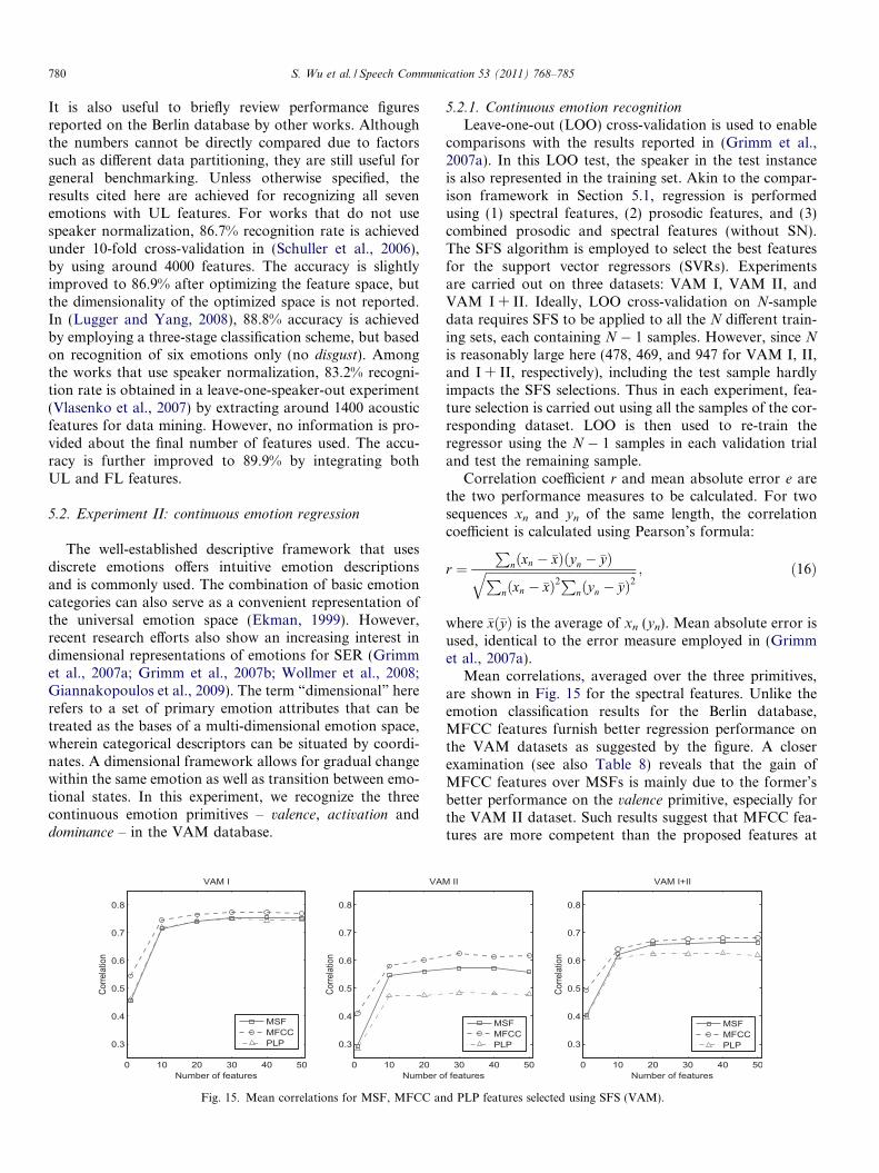
Mean correlations, averaged over the three primitives,are shown in Fig. 15 for the spectral features. Unlike theemotion classification results for the Berlin database,MFCC features furnish better regression performance onthe VAM datasets as suggested by the figure. A closerexamination (see also Table 8) reveals that the gain ofMFCC features over MSFs is mainly due to the former’sbetter performance on the valence primitive, especially forthe VAM II dataset. Such results suggest that MFCC fea-tures are more competent than the proposed features at

d PLP features selected using SFS (VAM).

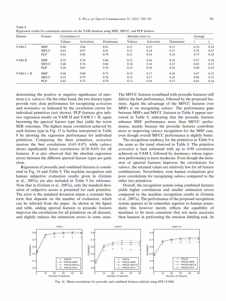
Table 8Regression results for continuous emotions on the VAM database using MSF, MFCC, and PLP features.

Dataset Feature Correlation (r) Absolute error (e) Average

Valence Activation Dominance Valence Activation Dominance �r �e

VAM I MSF 0.60 0.86 0.81 0.11 0.15 0.15 0.76 0.14MFCC 0.65 0.87 0.81 0.11 0.14 0.15 0.78 0.13PLP 0.61 0.86 0.79 0.11 0.16 0.16 0.75 0.14

VAM II MSF 0.32 0.74 0.66 0.15 0.16 0.16 0.57 0.16MFCC 0.46 0.74 0.68 0.14 0.16 0.15 0.63 0.15PLP 0.26 0.63 0.59 0.15 0.18 0.16 0.49 0.16

VAM I + II MSF 0.46 0.80 0.75 0.13 0.17 0.16 0.67 0.15MFCC 0.52 0.79 0.74 0.13 0.17 0.16 0.68 0.15PLP 0.42 0.75 0.70 0.13 0.18 0.17 0.62 0.16


determining the positive or negative significance of emo-tions (i.e. valence). On the other hand, the two feature typesprovide very close performance for recognizing activation

and dominance as indicated by the correlation curves forindividual primitives (not shown). PLP features give infe-rior regression results on VAM II and VAM I + II, againbecoming the spectral feature type that yields the worstSER outcomes. The highest mean correlation achieved byeach feature type in Fig. 15 is further interpreted in Table8 by showing the regression performance for individualprimitives. Comparing the three primitives, activation

receives the best correlations (0.63–0.87), while valence

shows significantly lower correlations (0.26–0.65) for allfeatures. It is also observed that the absolute regressionerrors between the different spectral feature types are quiteclose.

Regression of prosodic and combined features is consid-ered in Fig. 16 and Table 9. The machine recognition andhuman subjective evaluation results given in (Grimmet al., 2007a) are also included in Table 9 for reference.Note that in (Grimm et al., 2007a), only the standard devi-ation of subjective scores is presented for each primitive.The error is the standard deviation minus a constant biasterm that depends on the number of evaluators, whichcan be inferred from the paper. As shown in the figureand table, adding spectral features to prosodic featuresimproves the correlations for all primitives on all datasets,and slightly reduces the estimation errors in some cases.

Fig. 16. Mean correlations for prosodic and com

The MFCC features (combined with prosodic features) stilldeliver the best performance, followed by the proposed fea-tures. Again the advantage of the MFCC features overMSFs is on recognizing valence. The performance gapsbetween MSFs and MFCC features in Table 8 appear nar-rowed in Table 9, indicating that the prosodic featuresenhance MSF performance more than MFCC perfor-mance, mainly because the prosodic features contributemore to improving valence recognition for the MSF case,even though overall MFCC performance is slightly better.

The recognition tendency for the primitives in Table 9 isthe same as the trend observed in Table 8. The primitiveactivation is best estimated with up to 0.90 correlationachieved on VAM I, followed by dominance whose regres-sion performance is more moderate. Even though the inclu-sion of spectral features improves the correlations forvalence, the attained values are relatively low for all featurecombinations. Nevertheless, even human evaluations givepoor correlations for recognizing valence compared to theother two primitives.

Overall, the recognition system using combined featuresyields higher correlations and smaller estimation errorscompared to the machine recognition results in (Grimmet al., 2007a). The performance of the proposed recognitionsystem appears to be somewhat superior to human assess-ment; this however merely reflects the capability ofmachines to be more consistent (but not more accurate)than humans in performing the emotion labeling task. In

bined features selected using SFS (VAM).

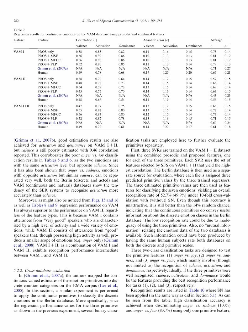
Table 9Regression results for continuous emotions on the VAM database using prosodic and combined features.

Dataset Feature Correlation (r) Absolute error (e) Average

Valence Activation Dominance Valence Activation Dominance �r �e

VAM I PROS only 0.58 0.85 0.82 0.11 0.16 0.15 0.75 0.14PROS + MSF 0.66 0.90 0.86 0.10 0.13 0.13 0.81 0.12PROS + MFCC 0.66 0.90 0.86 0.10 0.13 0.13 0.81 0.12PROS + PLP 0.62 0.90 0.85 0.11 0.13 0.14 0.79 0.13Grimm et al. (2007a) N/A N/A N/A N/A N/A N/A 0.71 0.27Human 0.49 0.78 0.68 0.17 0.25 0.20 0.65 0.21

VAM II PROS only 0.38 0.70 0.64 0.14 0.17 0.15 0.57 0.15PROS + MSF 0.48 0.78 0.73 0.14 0.15 0.14 0.66 0.14PROS + MFCC 0.54 0.79 0.73 0.13 0.15 0.14 0.69 0.14PROS + PLP 0.45 0.75 0.70 0.14 0.16 0.14 0.63 0.15Grimm et al. (2007a) N/A N/A N/A N/A N/A N/A 0.43 0.23Human 0.48 0.66 0.54 0.11 0.19 0.14 0.56 0.15

VAM I+II PROS only 0.47 0.77 0.75 0.13 0.17 0.15 0.66 0.15PROS + MSF 0.55 0.82 0.80 0.13 0.15 0.14 0.72 0.14PROS + MFCC 0.56 0.83 0.80 0.12 0.15 0.14 0.73 0.14PROS + PLP 0.52 0.82 0.78 0.13 0.16 0.15 0.71 0.15Grimm et al. (2007a) N/A N/A N/A N/A N/A N/A 0.60 0.24Human 0.49 0.72 0.61 0.14 0.22 0.17 0.61 0.18


(Grimm et al., 2007b), good estimation results are alsoachieved for activation and dominance on VAM I + II,but valence is still poorly estimated with 0.46 correlationreported. This corroborates the poor anger vs. joy classifi-cation results in Tables 5 and 6, as the two emotions arewith the same activation level but opposite valence. Sinceit has also been shown that anger vs. sadness, emotionswith opposite activation but similar valence, can be sepa-rated very well, both the Berlin (discrete and acted) andVAM (continuous and natural) databases show the ten-dency of the SER systems to recognize activation moreaccurately than valence.

Moreover, as might also be noticed from Figs. 15 and 16as well as Tables 8 and 9, regression performance on VAMI is always superior to the performance on VAM II, regard-less of the feature types. This is because VAM I containsutterances from “very good” speakers who are character-ized by a high level of activity and a wide variety of emo-tions, while VAM II consists of utterances from “good”speakers that, though possessing high activity as well, pro-duce a smaller scope of emotions (e.g. anger only) (Grimmet al., 2008). VAM I + II, as a combination of VAM I andVAM II, exhibits recognition performance intermediatebetween VAM I and VAM II.

5.2.2. Cross-database evaluation

In (Grimm et al., 2007a), the authors mapped the con-tinuous-valued estimates of the emotion primitives into dis-crete emotion categories on the EMA corpus (Lee et al.,2005). In this section, a similar experiment is performedto apply the continuous primitives to classify the discreteemotions in the Berlin database. More specifically, sincethe regression performance varies for the three primitivesas shown in the previous experiment, several binary classi-

fication tasks are employed here to further evaluate theprimitives separately.

First, three SVRs are trained on the VAM I + II datasetusing the combined prosodic and proposed features, onefor each of the three primitives. Each SVR uses the set offeatures selected by SFS on VAM I + II that yield the high-est correlation. The Berlin database is then used as a sepa-rate source for evaluation, where each file is assigned threepredicted primitive values by the three trained regressors.The three estimated primitive values are then used as fea-tures for classifying the seven emotions, yielding an overallrecognition rate of 52.7% (49.9%) under 10-fold cross-val-idation with (without) SN. Even though this accuracy isunattractive, it is still better than the 14% random chance,indicating that the continuous primitives do convey usefulinformation about the discrete emotion classes in the Berlindatabase. The low recognition rate could be due to inade-quacy of using the three primitives. Also, no “mutual infor-mation” relating the emotion data of the two databases isavailable. Such information could have been produced byhaving the same human subjects rate both databases onboth the discrete and primitive scales.

Three two-class classification tasks are designed to testthe primitive features: (1) anger vs. joy, (2) anger vs. sad-

ness, and (3) anger vs. fear, which mainly involve (thoughnot limited to) the recognition of valence, activation, anddominance, respectively. Ideally, if the three primitives werewell recognized, valence, activation, and dominance wouldbe the features providing the best recognition performancefor tasks (1), (2), and (3), respectively.

Recognition results are listed in Table 10 where SN hasbeen applied (in the same way as did in Section 5.1). As canbe seen from the table, high classification accuracy isachieved when discriminating anger vs. sadness (100%)and anger vs. fear (83.7%) using only one primitive feature,

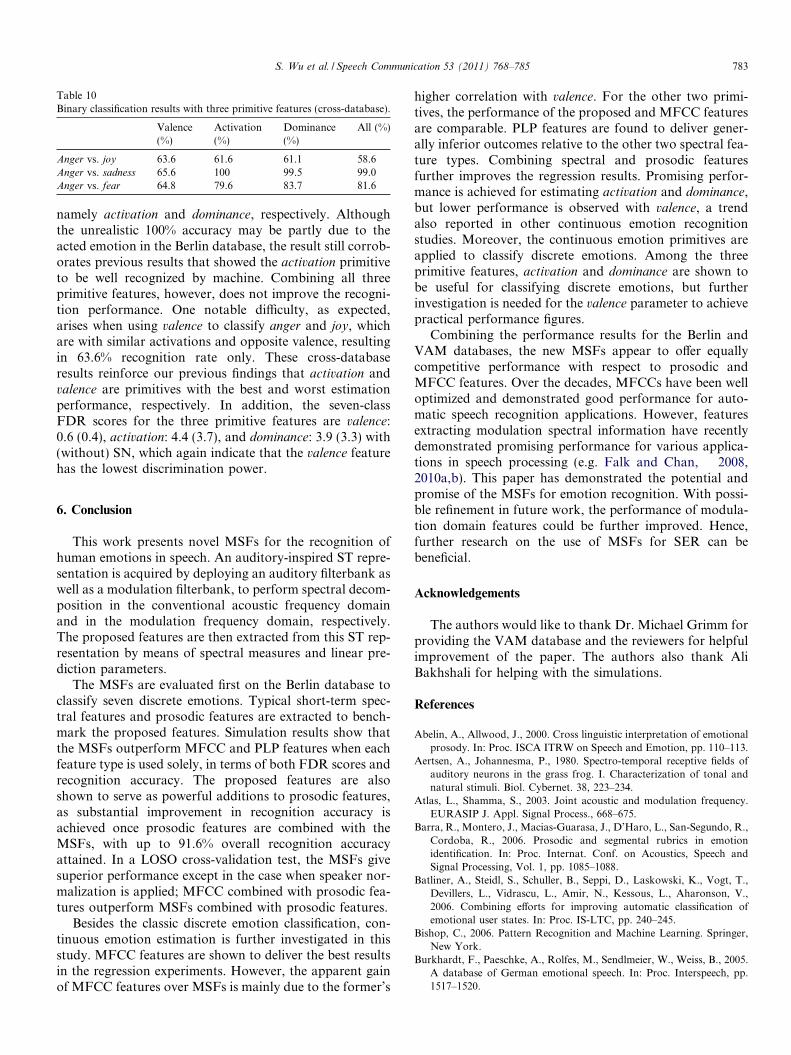
Table 10Binary classification results with three primitive features (cross-database).

Valence(%)

Activation(%)

Dominance(%)

All (%)

Anger vs. joy 63.6 61.6 61.1 58.6Anger vs. sadness 65.6 100 99.5 99.0Anger vs. fear 64.8 79.6 83.7 81.6


namely activation and dominance, respectively. Althoughthe unrealistic 100% accuracy may be partly due to theacted emotion in the Berlin database, the result still corrob-orates previous results that showed the activation primitiveto be well recognized by machine. Combining all threeprimitive features, however, does not improve the recogni-tion performance. One notable difficulty, as expected,arises when using valence to classify anger and joy, whichare with similar activations and opposite valence, resultingin 63.6% recognition rate only. These cross-databaseresults reinforce our previous findings that activation andvalence are primitives with the best and worst estimationperformance, respectively. In addition, the seven-classFDR scores for the three primitive features are valence:0.6 (0.4), activation: 4.4 (3.7), and dominance: 3.9 (3.3) with(without) SN, which again indicate that the valence featurehas the lowest discrimination power.

6. Conclusion

This work presents novel MSFs for the recognition ofhuman emotions in speech. An auditory-inspired ST repre-sentation is acquired by deploying an auditory filterbank aswell as a modulation filterbank, to perform spectral decom-position in the conventional acoustic frequency domainand in the modulation frequency domain, respectively.The proposed features are then extracted from this ST rep-resentation by means of spectral measures and linear pre-diction parameters.

The MSFs are evaluated first on the Berlin database toclassify seven discrete emotions. Typical short-term spec-tral features and prosodic features are extracted to bench-mark the proposed features. Simulation results show thatthe MSFs outperform MFCC and PLP features when eachfeature type is used solely, in terms of both FDR scores andrecognition accuracy. The proposed features are alsoshown to serve as powerful additions to prosodic features,as substantial improvement in recognition accuracy isachieved once prosodic features are combined with theMSFs, with up to 91.6% overall recognition accuracyattained. In a LOSO cross-validation test, the MSFs givesuperior performance except in the case when speaker nor-malization is applied; MFCC combined with prosodic fea-tures outperform MSFs combined with prosodic features.

Besides the classic discrete emotion classification, con-tinuous emotion estimation is further investigated in thisstudy. MFCC features are shown to deliver the best resultsin the regression experiments. However, the apparent gainof MFCC features over MSFs is mainly due to the former’s

higher correlation with valence. For the other two primi-tives, the performance of the proposed and MFCC featuresare comparable. PLP features are found to deliver gener-ally inferior outcomes relative to the other two spectral fea-ture types. Combining spectral and prosodic featuresfurther improves the regression results. Promising perfor-mance is achieved for estimating activation and dominance,but lower performance is observed with valence, a trendalso reported in other continuous emotion recognitionstudies. Moreover, the continuous emotion primitives areapplied to classify discrete emotions. Among the threeprimitive features, activation and dominance are shown tobe useful for classifying discrete emotions, but furtherinvestigation is needed for the valence parameter to achievepractical performance figures.

Combining the performance results for the Berlin andVAM databases, the new MSFs appear to offer equallycompetitive performance with respect to prosodic andMFCC features. Over the decades, MFCCs have been welloptimized and demonstrated good performance for auto-matic speech recognition applications. However, featuresextracting modulation spectral information have recentlydemonstrated promising performance for various applica-tions in speech processing (e.g. Falk and Chan, 2008,2010a,b). This paper has demonstrated the potential andpromise of the MSFs for emotion recognition. With possi-ble refinement in future work, the performance of modula-tion domain features could be further improved. Hence,further research on the use of MSFs for SER can bebeneficial.

Acknowledgements

The authors would like to thank Dr. Michael Grimm forproviding the VAM database and the reviewers for helpfulimprovement of the paper. The authors also thank AliBakhshali for helping with the simulations.

References

Abelin, A., Allwood, J., 2000. Cross linguistic interpretation of emotionalprosody. In: Proc. ISCA ITRW on Speech and Emotion, pp. 110–113.

Aertsen, A., Johannesma, P., 1980. Spectro-temporal receptive fields ofauditory neurons in the grass frog. I. Characterization of tonal andnatural stimuli. Biol. Cybernet. 38, 223–234.

Atlas, L., Shamma, S., 2003. Joint acoustic and modulation frequency.EURASIP J. Appl. Signal Process., 668–675.

Barra, R., Montero, J., Macias-Guarasa, J., D’Haro, L., San-Segundo, R.,Cordoba, R., 2006. Prosodic and segmental rubrics in emotionidentification. In: Proc. Internat. Conf. on Acoustics, Speech andSignal Processing, Vol. 1, pp. 1085–1088.

Batliner, A., Steidl, S., Schuller, B., Seppi, D., Laskowski, K., Vogt, T.,Devillers, L., Vidrascu, L., Amir, N., Kessous, L., Aharonson, V.,2006. Combining efforts for improving automatic classification ofemotional user states. In: Proc. IS-LTC, pp. 240–245.

Bishop, C., 2006. Pattern Recognition and Machine Learning. Springer,New York.

Burkhardt, F., Paeschke, A., Rolfes, M., Sendlmeier, W., Weiss, B., 2005.A database of German emotional speech. In: Proc. Interspeech, pp.1517–1520.


Busso, C., Lee, S., Narayanan, S., 2009. Analysis of emotionally salientaspects of fundamental frequency for emotion detection. IEEE Trans.Audio Speech Language Process. 17, 582–596.

Chang, C.-C., Lin, C.-J., 2009. LIBSVM: A library for support vectormachines. Tech. rep., Department of Computer Science, NationalTaiwan University. Software available at: <http://www.csie.ntu.e-du.tw/cjlin/libsvm>.

Chih, T., Ru, P., Shamma, S., 2005. Multiresolution spectrotemporalanalysis of complex sounds. J. Acoust. Soc. Amer. 118, 887–906.

Clavel, C., Vasilescu, I., Devillers, L., Richard, G., Ehrette, T., 2008. Fear-type emotion recognition for future audio-based surveillance systems.Speech Commun. 50, 487–503.

Cowie, R., Douglas-Cowie, E., 1996. Automatic statistical analysis of thesignal and prosodic signs of emotion in speech. In: Proc. Internat.Conf. on Spoken Language Processing, Vol. 3, pp. 1989–1992.

Cowie, R., Douglas-Cowie, E., Tsapatsoulis, N., Votsis, G., Kollias, S.,Fellenz, W., Taylor, J., 2001. Emotion recognition in human–computer interaction. IEEE Signal Process. Mag. 18, 32–80.

Davis, S., Mermelstein, P., 1980. Comparison of parametric representa-tions for monosyllabic word recognition in continuously spokensentences. IEEE Trans. Audio Speech Language Process. 28, 357–366.

Depireux, D., Simon, J., Klein, D., Shamma, S., 2001. Spectro-temporalresponse field characterization with dynamic ripples in ferret primaryauditory cortex. J. Neurophysiol. 85, 1220–1234.

Douglas-Cowie, E., Campbell, N., Cowie, R., Roach, P., 2003. Emotionalspeech: Towards a new generation of databases. Speech Commun. 40,33–60.

Ekman, P., 1999. Basic Emotions. John Wiley, New York, pp. 45–60.Ewert, S., Dau, T., 2000. Characterizing frequency selectivity for envelope

fluctuations. J. Acoust. Soc. Amer. 108, 1181–1196.Falk, T.H., Chan, W.-Y., 2008. A non-intrusive quality measure of

dereverberated speech. In: Proc. Internat. Workshop for AcousticEcho and Noise Control.

Falk, T.H., Chan, W.-Y., 2010a. Modulation spectral features for robustfar-field speaker identification. IEEE Trans. Audio Speech LanguageProcess. 18, 90–100.

Falk, T.H., Chan, W.-Y., 2010b. Temporal dynamics for blind measure-ment of room acoustical parameters. IEEE Trans. Instrum. Meas. 59,978–989.

Fletcher, H., 1940. Auditory patterns. Rev. Modern Phys. 12, 47–65.Giannakopoulos, T., Pikrakis, A., Theodoridis, S., 2009. A dimensional

approach to emotion recognition of speech from movies. In: Proc.Internat. Conf. on Acoustics, Speech and Signal Processing, pp. 65–68.

Glasberg, B., Moore, B., 1990. Derivation of auditory filter shapes fromnotched-noise data. Hearing Res. 47, 103–138.

Grimm, M., Kroschel, K., Mower, E., Narayanan, S., 2007a. Primitives-based evaluation and estimation of emotions in speech. SpeechCommun. 49, 787–800.

Grimm, M., Kroschel, K., Narayanan, S., 2007b. Support vectorregression for automatic recognition of spontaneous emotions inspeech. In: Proc. Internat. Conf. on Acoustics, Speech and SignalProcessing, Vol. 4, pp. 1085–1088.

Grimm, M., Kroschel, K., Narayanan, S., 2008. The Vera am MittagGerman audio-visual emotional speech database. In: Proc. Internat.Conf. on Multimedia & Expo, pp. 865–868.

Gunes, H., Piccard, M., 2007. Bi-modal emotion recognition fromexpressive face and body gestures. J. Network Comput. Appl. 30,1334–1345.

Hermansky, H., 1990. Perceptual linear predictive (PLP) analysis ofspeech. J. Acoust. Soc. Amer. 87, 1738–1752.

Hsu, C.-C., Chang, C.-C., Lin, C.-J., 2007. A practical guide to supportvector classification. Tech. rep., Department of Computer Science,National Taiwan University.

Intl. Telecom. Union, 1993. Objective measurement of active speech level.ITU-T P.56, Switzerland.

Intl. Telecom. Union, 1996. A silence compression scheme for G.729optimized for terminals conforming to ITU-T recommendation V.70.ITU-T G.729 Annex B, Switzerland.

Ishi, C., Ishiguro, H., Hagita, N., 2010. Analysis of the roles and thedynamics of breathy and whispery voice qualities in dialogue speech.EURASIP J. Audio Speech Music Process., article ID 528193, 12pages.

Kaiser, J., 1990. On a simple algorithm to calculate the ‘energy’ of a signal.In: Proc. Internat. Conf. on Acoustics, Speech and Signal Processing,Vol. 1, pp. 381–384.

Kanederaa, N., Araib, T., Hermanskyc, H., Pavel, M., 1999. On therelative importance of various components of the modulationspectrum for automatic speech recognition. Speech Commun. 28,43–55.

Kittler, J., 1978. Feature set search algorithms. Pattern Recognition SignalProcess., 41–60.

Lee, S., Yildirim, S., Kazemzadeh, A., Narayanan, S., 2005. Anarticulatory study of emotional speech production. In: Proc. Inter-speech, pp. 497–500.

Lugger, M., Yang, B., 2008. Cascaded emotion classification via psycho-logical emotion dimensions using a large set of voice qualityparameters. In: Proc. Internat. Conf. on Acoustics, Speech and SignalProcessing, Vol. 4, pp. 4945–4948.

Morgan, N., Zhu, Q., Stolcke, A., Sonmez, K., Sivadas, S., Shinozaki, T.,Ostendorf, M., Jain, P., Hermansky, H., Ellis, D., Doddington, G.,Chen, B., Cetin, O., Bourlard, H., Athineos, M., 2005. Pushing theenvelope – aside. IEEE Signal Process. Mag. 22, 81–88.

Mozziconacci, S., 2002. Prosody and emotions. In: Proc. Speech Prosody,pp. 1–9.

Nwe, T., Foo, S., De Silva, L., 2003. Speech emotion recognition usinghidden markov models. Speech Commun. 41, 603–623.

Picard, R., 1997. Affective Computing. The MIT Press.Rabiner, L., Juang, B., 1993. Fundamentals of Speech Recognition.

Prentice-Hall, Englewood Cliffs, NJ.Scherer, K., 2003. Vocal communication of emotion: A review of research

paradigms. Speech Commun. 40, 227–256.Scherer, S., Schwenker, F., Palm, G., 2007. Classifier fusion for emotion

recognition from speech. In: Proc. IET Internat. Conf. on IntelligentEnvironments, pp. 152–155.

Schuller, B., Seppi, D., Batliner, A., Maier, A., Steidl, S., 2006. Emotionrecognition in the noise applying large acoustic feature sets. In: Proc.Speech Prosody.

Schuller, B., Batliner, A., Seppi, D., Steidl, S., Vogt, T., Wagner, J.,Devillers, L., Vidrascu, L., Amir, N., Kessous, L., Aharonson, V.,2007a. The relevance of feature type for the automatic classification ofemotional user states: Low level descriptors and functionals. In: Proc.Interspeech, pp. 2253–2256.

Schuller, B., Seppi, D., Batliner, A., Maier, A., Steidl, S., 2007b. Towardsmore reality in the recognition of emotional speech. In: Proc.Internat. Conf. on Acoustics, Speech and Signal Processing, Vol. 4.pp. 941–944.

Shami, M., Verhelst, W., 2007. An evaluation of the robustness of existingsupervised machine learning approaches to the classification ofemotions in speech. Speech Commun. 49, 201–212.

Shamma, S., 2001. On the role of space and time in auditory processing.Trends Cogn. Sci. 5, 340–348.

Shamma, S., 2003. Encoding sound timbre in the auditory system. IETE J.Res. 49, 193–205.

Slaney, M., 1993. An efficient implementation of the Patterson–Holds-worth auditory filterbank. Tech. rep., Apple Computer, PerceptionGroup.

Sun, R., E., M., Torres, J., 2009. Investigating glottal parameters fordifferentiating emotional categories with similar prosodics. In: Proc.Internat. Conf. on Acoustics, Speech and Signal Processing, pp. 4509–4512.

Talkin, D., 1995. A robust algorithm for pitch tracking (RAPT). ElsevierScience, Speech Coding and Synthesis (Chapter 14).

Vapnik, V., 1995. The Nature of Statistical Learning Theory. Springer,New York.

Ververidis, D., Kotropoulos, C., 2006. Emotional speech recognition:Resources, features, and methods. Speech Commun. 48, 1162–1181.

http://www.csie.ntu.edu.tw/cjlin/libsvm

http://www.csie.ntu.edu.tw/cjlin/libsvm


Vlasenko, B., Schuller, B., Wendemuth, A., Rigoll, G., 2007. Combiningframe and turn-level information for robust recognition of emotionswithin speech. In: Proc. Interspeech, pp. 2225–2228.

Wollmer, M., Eyben, F., Reiter, S., Schuller, B., Cox, C., Douglas-Cowie,E., Cowie, R., 2008. Abandoning emotion classes – Towards contin-uous emotion recognition with modelling of long-range dependencies.In: Proc. Interspeech, pp. 597–600.

Wu, S., Falk, T., Chan, W.-Y., 2009. Automatic recognition of speechemotion using long-term spectro-temporal features. In: Proc. Internat.Conf. on Digital Signal Processing, pp. 1–6.

Zhou, G., Hansen, J., Kaiser, J., 2001. Nonlinear feature based classifi-cation of speech under stress. IEEE Trans. Audio Speech LanguageProcess. 9, 201–216.

automatic speech emotion recognition using …...automatic speech emotion recognition using...

Documents