UPTEC IT 13 011

Examensarbete 30 hpAugusti 2013

Automatic Segmentation of Skeleton in Whole-Body MR Images

Anders Hedström

Teknisk- naturvetenskaplig fakultet UTH-enheten Besöksadress: Ångströmlaboratoriet Lägerhyddsvägen 1 Hus 4, Plan 0 Postadress: Box 536 751 21 Uppsala Telefon: 018 – 471 30 03 Telefax: 018 – 471 30 00 Hemsida: http://www.teknat.uu.se/student

Abstract

Automatic Segmentation of Skeleton in Whole-BodyMR Images

Anders Hedström

Magnetic Resonance Imaging(MRI) has developed as a widespread technique toexamine various body parts and diagnose a wide range of diseases. MRI can often besuperior to other imaging techniques such as Computed Tomography(CT) since itdoes not use ionizing radiation and can give a clearer image of soft tissue. As MRIbecomes a more important part in medicine the demands on software to analyse theimages and extract useful information increases. Today medical image analysis can beused to localise tumours, measure brain substance and to isolate specific organs.Although much has happened in the field in recent years there is still little publishedabout segmentation of skeleton in MRI images, this might be because cortical boneneither contains fat nor water and thus gives a weak signal in MRI images. Skeletalsegmentation could still be useful to localise other body parts, to guide furtheranalysis of whole body images and to do attenuation correction in PET/MRI systems.This work aims to increase the knowledge about skeletal segmentation in fat andwater(FWI) MR images, and the goal is to produce a method that is flexible androbust enough to work on different MR machines with patients of various body types.This work implemented and evaluated two methods for skeletal segmentation in fatand water MR images. The first method divided the body into different regions andsegmented each region with a region-specific algorithm and the other methodconsisted of a filter that detect patterns in the proximity of bone.The evaluation used reference segmentations performed with the programSmartPaint, and overlap with the automatic method was measured. Subjects used inthis work originated from two studies, one on small patients and one on largerpatients, thus giving an indication of how well the methods work on a population withlarge variance.Results show that the filter method produce a more accurate result than the bodydivision method. The body division method had an average dice coefficient of 0.836,over segmentation ratio of 0.225 and under segmentation ratio of 0.120. The filtermethod had a dice coefficient of 0.944 and over and under segmentation rates wereboth 0.055.Both methods needed post processing in order to get a result that minimised theover segmentation in order to achieve an acceptable result. Neither of the methodsallows accurate assessment of bone volume, but an approximation might be possiblewith the filter method.This project has shown that it is possible to segment skeleton in whole body MRimages with a decent result without using either registration or deformable models.More advanced methods will most likely be needed to minimise the oversegmentation and increase segmentation accuracy.

Tryckt av: Reprocentralen ITCISSN: 1401-5749, UPTEC IT13 011Examinator: Lars-Åke NordénÄmnesgranskare: Joel KullbergHandledare: Robin Strand

Sammanfattning

Magnetisk Resonans Tomografi (MRT) har snabbt utvecklats till en teknik som används för attundersöka olika kroppsdelar och diagnostisera en mängd sjukdomar. MRT är ofta en lämpli-gare bildtagningsteknik än andra tekniker som datortomografi(CT) då det inte använder nå-gon joniserad strålning och ger tydligare bilder av mjuk vävnad. Allt eftersom att teknikenutvecklas och blir mer använd ökar kraven på mjukvara som kan analysera bilderna och extra-hera värdefull information. Idag används medicinsk bildanalys bland annat för att lokaliseratumörer, mäta hjärnsubstans och för att isolera specifika organ.

Det finns fortfarande relativt få publicerade artiklar om segmentering av skelett i MRTbilder, detta kan bero på att kortikal benvävnad varken innehåller mycket fett eller vatten ochger därför svag signal i MRT bilder. Segmentering av skelett kan ändå vara till stor hjälpför att lokalisera andra kroppsdelar, för att hjälpa analys av helkroppsbilder och för att hjälpaattenueringskorrigering i PET-MRT data.

Det här arbetet syftar på att utveckla en helautomatisk skelettsegmentering av helkropps,fett och vatten magnetresonans bilder. Metoden ska vara tillräckligt flexibel och robust föratt fungera acceptabelt på bilder med olika inställningar på MR-maskinen och för patien-ter/försökspersoner med olika kroppsstorlek.

I det här arbetet utvecklades och utvärderades två metoder, den ena metoden utgår frånen kroppsindelning där varje kroppsdel har en tillhörande segmenteringsfunktion, den andrametoden består av ett filter som lokaliserar mönster som finns i områden runt skelett.

Utvärderingen använde manuella segmenteringar av MRT undersökningar som referens.Försökspersonerna och patienterna är tagna från två studier, en studie på större försökspersoneroch en på smalare, på så sätt ges en indikation på hur funktionerna fungerar för en populationmed stor varians.

Resultatet visade att filtermetoden var mer precis och noggrann än kroppsindelningsmeto-den. Kroppsindelningsmetoden hade ett genomsnittligt dice värde på 0,836, Översegmenter-ingsgrad på 0,225 och undersegmenteringsgrad på 0,120. Filtermetoden hade i snitt ett dice-värde på 0,944 och både över och under- segmenteringsgraden låg på ungefär 0,055. Bådametoderna kräver att efterbehandling används för att få ett resultat som inte har för mycketöversegmentering, och även med efterbehandling sågs översegmentering vara ett problem.Över och under- segmentering leder till att metodernas stabilitet inte är optimal, men det ärmöjligt att få en ungefärlig uppskattning på patientens skelett-volym.

Det här projektet visade att det går att segmentera skelett i helkropps MRI-bilder med rela-tivt bra resultat utan att använda sig av registrering eller deformerbara modeller, men att meravancerade metoder måste användas om ett resultat fritt från översegmentering behövs.

Contents

Sammanfattning . . . . . . . . . . . . . . . . . . . . . . . . . . . . . . . . . . . . . . . . . . . . . . . . . . . . . . . . . . . . . . . . . . . . . . . . . . . . . . . . . . . . . . . . . . . . . . . . . . . . . . . . . . . . . . . . . . . . . . . . . . . . . i

1 Introduction . . . . . . . . . . . . . . . . . . . . . . . . . . . . . . . . . . . . . . . . . . . . . . . . . . . . . . . . . . . . . . . . . . . . . . . . . . . . . . . . . . . . . . . . . . . . . . . . . . . . . . . . . . . . . . . . . . . . . . . . . . . . . 51.1 Background . . . . . . . . . . . . . . . . . . . . . . . . . . . . . . . . . . . . . . . . . . . . . . . . . . . . . . . . . . . . . . . . . . . . . . . . . . . . . . . . . . . . . . . . . . . . . . . . . . . . . . . . . . . . . . . . . . 51.2 Purpose and goal . . . . . . . . . . . . . . . . . . . . . . . . . . . . . . . . . . . . . . . . . . . . . . . . . . . . . . . . . . . . . . . . . . . . . . . . . . . . . . . . . . . . . . . . . . . . . . . . . . . . . . . . . 51.3 Project outline and limitations . . . . . . . . . . . . . . . . . . . . . . . . . . . . . . . . . . . . . . . . . . . . . . . . . . . . . . . . . . . . . . . . . . . . . . . . . . . . . . . . . . . . 61.4 Similar work . . . . . . . . . . . . . . . . . . . . . . . . . . . . . . . . . . . . . . . . . . . . . . . . . . . . . . . . . . . . . . . . . . . . . . . . . . . . . . . . . . . . . . . . . . . . . . . . . . . . . . . . . . . . . . . . 6

2 Introduction to image processing . . . . . . . . . . . . . . . . . . . . . . . . . . . . . . . . . . . . . . . . . . . . . . . . . . . . . . . . . . . . . . . . . . . . . . . . . . . . . . . . . . . . . . . . . . 82.1 Description of image processing . . . . . . . . . . . . . . . . . . . . . . . . . . . . . . . . . . . . . . . . . . . . . . . . . . . . . . . . . . . . . . . . . . . . . . . . . . . . . . . . 82.2 Segmentation . . . . . . . . . . . . . . . . . . . . . . . . . . . . . . . . . . . . . . . . . . . . . . . . . . . . . . . . . . . . . . . . . . . . . . . . . . . . . . . . . . . . . . . . . . . . . . . . . . . . . . . . . . . . . . . 9

2.2.1 Thresholding . . . . . . . . . . . . . . . . . . . . . . . . . . . . . . . . . . . . . . . . . . . . . . . . . . . . . . . . . . . . . . . . . . . . . . . . . . . . . . . . . . . . . . . . . . . . . . . . . 92.2.2 Morphological image processing . . . . . . . . . . . . . . . . . . . . . . . . . . . . . . . . . . . . . . . . . . . . . . . . . . . . . . . . . . . . . . 102.2.3 Clustering . . . . . . . . . . . . . . . . . . . . . . . . . . . . . . . . . . . . . . . . . . . . . . . . . . . . . . . . . . . . . . . . . . . . . . . . . . . . . . . . . . . . . . . . . . . . . . . . . . . . 112.2.4 Model based . . . . . . . . . . . . . . . . . . . . . . . . . . . . . . . . . . . . . . . . . . . . . . . . . . . . . . . . . . . . . . . . . . . . . . . . . . . . . . . . . . . . . . . . . . . . . . . . 12

3 Introduction to magnetic resonance imaging . . . . . . . . . . . . . . . . . . . . . . . . . . . . . . . . . . . . . . . . . . . . . . . . . . . . . . . . . . . . . . . . . . . . . . 13

4 Methodology . . . . . . . . . . . . . . . . . . . . . . . . . . . . . . . . . . . . . . . . . . . . . . . . . . . . . . . . . . . . . . . . . . . . . . . . . . . . . . . . . . . . . . . . . . . . . . . . . . . . . . . . . . . . . . . . . . . . . . . . . 144.1 MRI images . . . . . . . . . . . . . . . . . . . . . . . . . . . . . . . . . . . . . . . . . . . . . . . . . . . . . . . . . . . . . . . . . . . . . . . . . . . . . . . . . . . . . . . . . . . . . . . . . . . . . . . . . . . . . . . 144.2 Subjects . . . . . . . . . . . . . . . . . . . . . . . . . . . . . . . . . . . . . . . . . . . . . . . . . . . . . . . . . . . . . . . . . . . . . . . . . . . . . . . . . . . . . . . . . . . . . . . . . . . . . . . . . . . . . . . . . . . . . . 164.3 Evaluation . . . . . . . . . . . . . . . . . . . . . . . . . . . . . . . . . . . . . . . . . . . . . . . . . . . . . . . . . . . . . . . . . . . . . . . . . . . . . . . . . . . . . . . . . . . . . . . . . . . . . . . . . . . . . . . . . . 174.4 Software used . . . . . . . . . . . . . . . . . . . . . . . . . . . . . . . . . . . . . . . . . . . . . . . . . . . . . . . . . . . . . . . . . . . . . . . . . . . . . . . . . . . . . . . . . . . . . . . . . . . . . . . . . . . . 184.5 Problem with sampling . . . . . . . . . . . . . . . . . . . . . . . . . . . . . . . . . . . . . . . . . . . . . . . . . . . . . . . . . . . . . . . . . . . . . . . . . . . . . . . . . . . . . . . . . . . . . 214.6 Segmentation method1 - Body parts . . . . . . . . . . . . . . . . . . . . . . . . . . . . . . . . . . . . . . . . . . . . . . . . . . . . . . . . . . . . . . . . . . . . . . . . 21

4.6.1 Dividing the body . . . . . . . . . . . . . . . . . . . . . . . . . . . . . . . . . . . . . . . . . . . . . . . . . . . . . . . . . . . . . . . . . . . . . . . . . . . . . . . . . . . . . . . 214.6.2 Segmenting each body part . . . . . . . . . . . . . . . . . . . . . . . . . . . . . . . . . . . . . . . . . . . . . . . . . . . . . . . . . . . . . . . . . . . . . . . . 23

4.7 Segmentation method2 - Filter . . . . . . . . . . . . . . . . . . . . . . . . . . . . . . . . . . . . . . . . . . . . . . . . . . . . . . . . . . . . . . . . . . . . . . . . . . . . . . . . . 274.7.1 Filter idea . . . . . . . . . . . . . . . . . . . . . . . . . . . . . . . . . . . . . . . . . . . . . . . . . . . . . . . . . . . . . . . . . . . . . . . . . . . . . . . . . . . . . . . . . . . . . . . . . . . . 274.7.2 Description . . . . . . . . . . . . . . . . . . . . . . . . . . . . . . . . . . . . . . . . . . . . . . . . . . . . . . . . . . . . . . . . . . . . . . . . . . . . . . . . . . . . . . . . . . . . . . . . . . 284.7.3 Determining parameters . . . . . . . . . . . . . . . . . . . . . . . . . . . . . . . . . . . . . . . . . . . . . . . . . . . . . . . . . . . . . . . . . . . . . . . . . . . . . 29

4.8 Post-processing . . . . . . . . . . . . . . . . . . . . . . . . . . . . . . . . . . . . . . . . . . . . . . . . . . . . . . . . . . . . . . . . . . . . . . . . . . . . . . . . . . . . . . . . . . . . . . . . . . . . . . . . . 304.8.1 Body mask . . . . . . . . . . . . . . . . . . . . . . . . . . . . . . . . . . . . . . . . . . . . . . . . . . . . . . . . . . . . . . . . . . . . . . . . . . . . . . . . . . . . . . . . . . . . . . . . . . 304.8.2 Intestine mask . . . . . . . . . . . . . . . . . . . . . . . . . . . . . . . . . . . . . . . . . . . . . . . . . . . . . . . . . . . . . . . . . . . . . . . . . . . . . . . . . . . . . . . . . . . . . 314.8.3 Trachea mask . . . . . . . . . . . . . . . . . . . . . . . . . . . . . . . . . . . . . . . . . . . . . . . . . . . . . . . . . . . . . . . . . . . . . . . . . . . . . . . . . . . . . . . . . . . . . . 31

5 Result . . . . . . . . . . . . . . . . . . . . . . . . . . . . . . . . . . . . . . . . . . . . . . . . . . . . . . . . . . . . . . . . . . . . . . . . . . . . . . . . . . . . . . . . . . . . . . . . . . . . . . . . . . . . . . . . . . . . . . . . . . . . . . . . . . . . . 335.1 Result - Body parts . . . . . . . . . . . . . . . . . . . . . . . . . . . . . . . . . . . . . . . . . . . . . . . . . . . . . . . . . . . . . . . . . . . . . . . . . . . . . . . . . . . . . . . . . . . . . . . . . . . . 335.2 Result - Filter . . . . . . . . . . . . . . . . . . . . . . . . . . . . . . . . . . . . . . . . . . . . . . . . . . . . . . . . . . . . . . . . . . . . . . . . . . . . . . . . . . . . . . . . . . . . . . . . . . . . . . . . . . . . . 36

6 Discussion and conclusion . . . . . . . . . . . . . . . . . . . . . . . . . . . . . . . . . . . . . . . . . . . . . . . . . . . . . . . . . . . . . . . . . . . . . . . . . . . . . . . . . . . . . . . . . . . . . . . . . . . 396.1 Discussion - Body parts method . . . . . . . . . . . . . . . . . . . . . . . . . . . . . . . . . . . . . . . . . . . . . . . . . . . . . . . . . . . . . . . . . . . . . . . . . . . . . . 39

6.2 Discussion - Filter method . . . . . . . . . . . . . . . . . . . . . . . . . . . . . . . . . . . . . . . . . . . . . . . . . . . . . . . . . . . . . . . . . . . . . . . . . . . . . . . . . . . . . . . 406.3 Conclusion . . . . . . . . . . . . . . . . . . . . . . . . . . . . . . . . . . . . . . . . . . . . . . . . . . . . . . . . . . . . . . . . . . . . . . . . . . . . . . . . . . . . . . . . . . . . . . . . . . . . . . . . . . . . . . . . . 416.4 Suggestions for future work . . . . . . . . . . . . . . . . . . . . . . . . . . . . . . . . . . . . . . . . . . . . . . . . . . . . . . . . . . . . . . . . . . . . . . . . . . . . . . . . . . . . . 42

References . . . . . . . . . . . . . . . . . . . . . . . . . . . . . . . . . . . . . . . . . . . . . . . . . . . . . . . . . . . . . . . . . . . . . . . . . . . . . . . . . . . . . . . . . . . . . . . . . . . . . . . . . . . . . . . . . . . . . . . . . . . . . . . . . . . 44

Appendix . . . . . . . . . . . . . . . . . . . . . . . . . . . . . . . . . . . . . . . . . . . . . . . . . . . . . . . . . . . . . . . . . . . . . . . . . . . . . . . . . . . . . . . . . . . . . . . . . . . . . . . . . . . . . . . . . . . . . . . . . . . . . . . . . . . . . 46

1. Introduction

1.1 BackgroundThis thesis was done at the Department of Radiology, Oncology and Radiation science at Up-psala University.

In recent years medical imaging has come to be a crucial part in modern medicine, this isindicated by the fact that imaging with computed tomography(CT) doubled between 1997and 2006 and imaging with magnetic resonance imaging(MRI) tripled during the same period[15]. Problems concerning the skeletal system is a common problem in medicine, especiallyamongst the elder, thus new and improved techniques to diagnose and image the skeletal sys-tem is constantly being developed. A problem is that most technologies currently used to imagebone in patients subjects them to radiation. Since radiation is related to health problems, thiscan reduce the amount of images gathered from patients. Magnetic resonance imaging on theother hand does not subject patients to radiation, and have no known health concerns. Thus itwould be advantageous if you could analyse bone with MRI images instead of X-ray or CT.

As new medical imaging technologies develops, image analysis techniques developes along-side them to be able to analyse these images. Segmentation is a key steps in image analysisand medical images have properties that can make them hard to segment, such as differenttissues having similar intensities, organs occluding and overlapping each other and humanshaving large variance in physique. These problems can be diminished somewhat by makingalgorithms that are specifically designed for medical images. By making these specialized al-gorithms you can take into account anatomy and physiology, and thus get more accurate andreliable results.

Medical image analysis have come to be an important field in healthcare, both in the treat-ment of patients and in research. This thesis aims to further the progress made with segmenta-tion of the human skeletal system in MRI images.

1.2 Purpose and goalThere is currently not much research being published on the segmentation of bone in MRIimages, this is partially because it is easier to see and segment bone in other image modalitieslike CT and X-ray. Even though CT images gives better images of the bone, segmentationwith MRI machines is still desirable since MRI images can be gathered without subjecting thepatient to radiation. Skeletal segmentation is also needed as it can help to correct attenuationon combined PET/MRI machines [14], which is useful as those machines become more readilyavailable. Most papers published on the segmentation of bone in MRI images also concentrateon parts of the body, and not the whole.

The main goal of this work is to create a fully automatic segmentation of the human skeletalsystem in whole-body MRI images. It investigated which methods were useful in achieving a

5

good segmentation result. The problems that exist when segmenting bone should be identifiedand where it is possible these problems should be solved or reduced. Different methods forevaluating the result of the segmentation should be considered and appropriate methods shouldbe used to investigate the results of the segmentations.

1.3 Project outline and limitationsThis thesis can be divided into two parts, a theoretical part and a practical part. The theoreticalpart consisted of studying the literature and analysing the MRI images to answer the followingquestions:

• Which methods have been used previously for segmentation of skeleton in MRI images?

• What other techniques could possibly be used?

• Which is the most effective way to evaluate the segmentation?

The practical part consisted of implementing the chosen algorithms found in the theoreticalparts and assessing the result of their performance. The implementation and evaluation wasdone iteratively wherever possible. Meaning that the first algorithm was implemented then thatalgorithm was evaluated, then the second algorithm was implemented and evaluated and so on.

A limitation in the project was that only a fix type of images were used, namely fat andwater images or images that are made by filtering those images. The resolution of the imagesis also a limitation, pixel resolution is typically 200-300 voxels in each of the x-, y- and z-axis.Even though that pixel resolution is normal for these types of images it can be hard to segmentsmall structures since the images are full-body and small objects might only be a couple ofvoxels large. There was also a limited dataset of images, which made it difficult to verify thatthe algorithms were robust over varying patients.

1.4 Similar workIn recent years much work has been done when it comes to the segmentation of medical im-ages, especially segmenting brains[7] , detecting tumours[10] and monitoring heart ventricles[6].Work on segmentation of skeleton has been done, but the majority of the work is done withCT images and not MRI images since CT gives a clearer view of skeleton. Most of the timeskeletal segmentation focuses on smaller parts of the body and not the whole skeletal system,most notably is segmentation of bones in the thigh and pelvis area[4][9] and segmentation ofthe skull[14].

Deformable models is one of the most commonly used method for segmenting medical im-ages, this is because the objects searched for within the human body has a know shape and thatinformation can be incorporated into the model. A downside with deformable models is thatthey can perform poorly if the patients anatomy differs greatly from the anatomy of the model,this can be a problem if the patient have broken bones or a skeletal disorder which deforms the

6

bones. It has been shown that an atlas constructed from European patients can perform poorlyon patients from Japans since their skeleton can differ from that of the European patients[8].Thus factors such as age, gender and ethnicity should be considered while constructing anatlas.

Machine learning approaches have also been used to segment skeleton[14]. Supervisedlearning methods can be used to train the segmentation to recognize skeleton in certain bodyparts. This requires that you have training examples, some of which are skeleton and somewhich are not. Machine learning can be used to construct segmentation algorithms which doesnot rely as much on intensity, which can be advantageous when segmenting skeleton sincebone and air have similar intensities.

Skeletal segmentation using morphological operations has been done [5]. The advantages ofusing morphology over deformable models are that the segmentation is usually not dependanton knowing the structure of the bones beforehand. Thus you can segment images from peoplewith bone deformations. Morphological operations also has the advantage of often being easierto implement and being more time efficient. The downside of morphological segmentation isthat the result is often not as accurate as deformable models, so if the segmentation needs ahigh degree of accuracy morphology might not work.

In conclusion we can see that several techniques are regularly used for segmenting medicalimages. Some of the most common being deformable models, morphological and machinelearning. All of these methods have pros and cons, and the preferred methods depends onwhat you want to achieve with the segmentation. For this projects several methods will beimplemented and tested to see which yields the best segmentation result.

7

2. Introduction to image processing

Two terms used in this thesis are image processing and image analysis. Image processing isany form of signal processing where the input data is an image and the output is either animage or parameters that describe some aspect of the image. A typical image processing taskcould be to filter an image to find edges, make it smoother or to enhance contrast. Imageanalysis on the other hand is the act of extracting meaningful information from an image,mainly using image processing techniques. Typical image analysis tasks include segmentation,object detection or motion detection. Fields where image analysis is commonly used includesmedicine, astronomy, robotics and computer security.

2.1 Description of image processingThere is a number of steps undertaken to solve an image analysis problem, they are as follows:

1. Image acquisition

2. Pre-processing

3. Segmentation

4. Feature extraction

5. Classification

In the image acquisition step you try to collect images with as good image quality and fewartefacts as possible. Pre-processing is about removing artefacts and making it a suitable rep-resentation for the segmentation step. The segmentation step, which this project focuses on,is about identifying and extracting areas of the image which are of particular interest. Featureextraction deals with extracting useful information from the segmented regions, if you segmenta liver you might extract its size and fat percentage. Classification draws conclusions from thedata extracted in the previous step, this classification might for instance state whether or notthe patient has cancer.

8

Figure 2.1: An illustration of the steps undertaken when solving an image processing task

2.2 SegmentationImage segmentation is the process of partitioning an image into several sub-regions. Each re-gion should correspond to an area of significance, such as an object or a boundary in the image.In this thesis the objects to be segmented are bones found in MRI images. There are numerouscriteria that can be used to determine if a pixel belongs to a particular segmentation region,some of the most often used are criteria are colour, intensity, texture and shape. It can oftenbe useful to use information from several images, for instance from different image acquiringtechniques or from different times when segmenting an image to get a better result. Usingseveral images has been compared to using several sensory organs to get more informationabout what it is experiencing [11]. The following subsections describe some image analysistechniques that is used in this project and other techniques commonly used to segment bone.

2.2.1 ThresholdingThresholding is one of the simplest and most commonly used techniques used for image seg-mentation. Thresholding relies on the assumption that an image can be divided into separateregions solely based on intensity values. The most common way of using thresholding is todivide the image into two regions depending on their intensity, one region that becomes thebackground and one region that becomes the object. To determine what cluster a pixel belongsto, you can use the following formula.x ⊂C1 i f intensity(x)>thresholdx ⊂C2 i f intensity(x)≤thresholdWhere x is the pixel and intensity(x) is the grayscale value for that pixel.

9

Figure 2.2: Full body MRI image and the same image thresholded

One problem with thresholding is choosing an appropriate threshold level. If you choose athreshold that is too low pixels that are supposed to be background gets labeled as being part ofthe objects, and if you choose a threshold that is too high pixels that should be the object getsmarked as background. There are way to automatically determine an appropriate threshold,like Otsu’s method [13], but these methods does not always give the threshold wanted so ahuman is sometimes needed to make sure the threshold is acceptable.

Thresholding can be extended to divide the image into more than two regions by havingseveral threshold values, and can also be extended to colour images by thresholding eachcolour value in the image (for instance the red, green and blue colour channels).

2.2.2 Morphological image processingMorphological image processing is a set of image processing techniques that transforms ob-jects in the image based on their shapes. Morphology is largely based on set theory andtopology and is typically done on binary images, but can also be used on grayscale images.Morphological techniques apply a structuring elements to the image and records whether thestructuring elements hit, miss or fits inside the objects in the image and transforms them ac-cordingly. Examples of how the strucuring element can fit, hit or miss the object is shown inimage 2.3

Basic morphological operations include dilation, erosion, closing, opening. Dilation checkswhether or not the structuring element hits the object, this increases the size of the object byadding pixels to the boundary of object. Erosion removes pixels at the boundary of the object,

10

Figure 2.3: An illustration of how round structuring elements(SE) can fit(green), hit(yellow)or miss(red) an object(blue)

this is done by checking whether or not the structuring element fit the object. The amount ofpixels added or removed depends on the shape and size of the structuring element. Closing isa dilation followed by an erosion, this removes small holes that exists in the image. Openingis an erosion followed by a dilation, this removes small objects that exists in the image. Thesemorphological operations are shown in image 2.4

Figure 2.4: An image of how erode, dilate, open and close affects the original object

2.2.3 ClusteringClustering is the process of assigning pixels into groups (clusters), so that the pixels in eachcluster is similar to other pixels in its own group, but dissimilar from pixels in other groups.Clustering is not a single algorithm but a group name for many different types of algorithmsthat have similar functionality. How to decide what constitutes each cluster can be a difficulttask, and there exists a variety of different metrics for deciding this. Some popular metrics aredistance, density, various statistical features in the data set or in images intensity. Clusteringalgorithms can be used in image analysis for both image segmentation and classification. Oneexample of a popular clustering algorithm is k-means, which works like this:

1. Choose K number of clustering centers

11

2. Assign each voxel to the cluster with the closest center

3. Calculate a new center for each cluster by averaging all the pixels in the cluster

4. Repeat 2 and 3 until no pixels change cluster

Fuzzy clustering is a term used to describe clustering algorithms where each voxel can havea degree of belonging to several of the clusters, not just one. Spatial Fuzzy c-means(SFCM)is an algorithm that is similar to a fuzzy version of k-means, but it also incorporates spatialinformation.

2.2.4 Model basedModel based segmentation works by finding objects in the image that resembles a model thathas previously been produced. It is assumed that the objects in the image have a similargeometry, intensity or texture. The model based approach relies on knowing the approximateshape or look of the objects you are looking for. Model based segmentation is frequently usedin medical imaging because anatomical information can be taken into account and the factthat medical images can be hard to segment with other techniques. It has been used to locatetumours, especially in brains[3][12], and to automatically segment the brain and its differentregions[7][16].

To do model-based segmentation you first need to align(register) the model to the objectwithin the image. After that you need to alter the model so that it has a higher resemblancethe object in the image, this can be achieved by applying forces to the model. The forces canbe dependent on the shape of the object, intensity of the object, or they can be internal andexternal forces to adjust how much the model can be altered. The recent literature focus alot on these deformable models as indicated by this statement, "State of the art methods inthe literature for knowledge-based segmentation involve active shape and appearance models,active contours and deformable templates and level-set based methods" [1].

Problems with model-based segmentation are that the registration needs to be very accuratein order for the model to deform correctly. The computational time can be high, and it can bedifficult to make accurate models that take into account variance between different images.

12

3. Introduction to magnetic resonance imaging

Magnetic resonance imaging uses magnetic fields and radio waves to gather two or three-dimensional interior images of the body. MRI machines primarily excite the hydrogen atomsfound in water or fat in the body, and since bone usually large quantities of fat and water,bones tend to have a weak signal on MRI scans. Because of MRIs weak signal in bone X-raysor CT scans are more commonly used for investigating bone injuries and diseases. MRI usesthe principle of nuclear magnetic resonance(NMR), a physical phenomenon in which nucleiof atoms absorbs and re-emits electromagnetic radiation when subjected to a magnetic field.

There are a number of steps in creating an MRI image, they are briefly explained below.1. Protons in atoms have randomly oriented spin, in MRI we are primarily concerned with

the spin of hydrogen found in water.2. When a magnetic field is applied, the spins align with the magnetic field and result in a

net magnetization.3. A radio frequency pulse is applied that affects the spin of the protons in the body being

studied.4. When the pulse stops the protons send out radio frequency signals as they return to their

original state.5. These radio frequency signals are picked up by radio frequency detectors and transformed

into an image.You choose what part of the body to examine by applying other magnetic fields to the body

that vary in strength across the body, this varying magnetic field is known as the gradient field.When the radio frequency pulse is applied to the body you can thus excite only certain nucleithat are only affected by a certain magnetic field. Thus you can choose what part of the bodyyou want to examine.

13

4. Methodology

4.1 MRI imagesIt is possible to do a number of different MRI scans and each type of scan has its own contrastand characteristics. The most commonly used scans are T1-weighted, T2-weighted and T ∗

2 -weighted. In T1-weighted scans fat has a bright intensity while water has a dark, in T2-weightedimages water is bright.

There are also a number of specialized MRI scans, examples of these include diffusion MRI,functional MRI (fMRI) and magnetic resonance angiography (MRA). These techniques makesit possible to image things not possible with standard imaging sequences, for instance MRA isused to generate pictures of the arteries and fMRI measures signal changes in the brain uponactivation.

Most techniques generate the images from fat and water molecules. Since fat and waterhave different resonance frequencies fat and water can be separated into two different images.The imaging technique where fat and water are separated is usually referred to as fat-waterimaging (FWI), these are the type of images that are used in this project. Some images havealso been computed from these water and fat images, such as the sum image which is the sumof water and fat in each voxel. Figure 4.1 show the three main types of images that were usedin this project, water-, fat- and sum-image.

Figure 4.1: From left to right, fat image, water image, sum image

The MRI scans were performed using a 1.5Tesla clinical scanner with a moving table.A special 3D gradient echo sequence collected three different images with different echotimes(TE) from each axial slice during continuous motion. The following imaging parameters

14

were used: TR 5.9 ms, TE 1.36/3.22/5.09 ms, flip angle 3 degrees, elementary signal sam-pling field of view (FOV) (in motion direction) 112 mm, virtual FOV 530x377x2000 mm3,and voxel size 2.07x2.07x8.00 mm3. The table speed was set to 6.5 mm/s resulting in a wholebody scan time of 5minutes 15seconds.

There are numerous image artefacts associated with MRI images. The artefacts that has beenthe most obvious in this project are partial volume effects, inhomogeneities in the magneticfield and motion blur.

Partial volume effects arise because of the fact that the resolution is not high enough soseveral types of tissues are included in the same voxel. Partial volume effects leads to edgesbetween different tissue types being blurred, this can be a big problem for full body imagessince the physical voxel size is quite large and the chances of different tissue types beinglocated in the same voxel is quite high. Partial volume effects can be reduced by decreasingthe physical size of each voxel.

Inhomogeneities in the magnetic field of the MRI scanner can cause the image to havedifferent intensities in different locations of the image, the left side of the image might forinstance have a higher intensity than the right side. The images used in this study have beencorrected to remove as much of these inhomogeneities as possible, but they can still be visiblein some images.

Motion artefacts are caused when a subject moves while the MRI scan is ongoing. Most ofthe images in this study does not have any major motion artefacts, but they can sometimes beseen in the abdomen of the subjects.

Three dimensional images can be viewed from several different planes, in this thesis coro-nal plane is assumed unless otherwise stated, the coronal plane divides the body into front andback sections. When x-coordinates are discussed they refer to the coordinates that goes fromleft to right in the image, y-coordinates refer to coordinates that goes from top to bottom andz-coordinates refer to the next or previous image in the image sequence. Other ways to viewimages is in the axial plane (top to bottom) and sagittal plane (left to right). Figure 4.2 is anexample of images viewed in the coronal plane.

15

Figure 4.2: An image of fat viewed in the coronal plane

4.2 SubjectsThe subjects in this paper were taken from two different studies, Lipogain and Gastric Bypass(GBP). Lipogain consisted of healthy volunteers between the ages of 20 and 36 who had aBMI index between 18 and 27. During the Lipogain study the subjects were asked to eatcupcakes in order to gain weight. The volunteers were scanned twice, once before startingeating the cupcakes and once after having added cupcakes to their diets. The Lipogain studysubjects thus gives a good indication of how the functions implemented works on subjects withnormal weight. GBP consisted of female patients who were going to undergo gastric bypasssurgery. They had a higher BMI than the Lipogain subjects, and thus gives an indication ofhow the method works for larger subjects. Only a subset of the subjects from these studieswere included in the evaluation of the methods developed. Table 4.1 shows the data for thefirst scans in each of the Lipogain and GBP studies.

n Age BMI Weight Sex(Women:Men)

Lipogain 37 26.9 20.7 65.4 11:26

GBP 15 34.7 ± 7.88 42.9 ± 3.02 121.3 ± 13.4 15:0

Table 4.1: Subject statistics from the two studies

16

4.3 EvaluationSeveral methods for the evaluation were considered, including visually judging the segmen-tation and creating manual reference segmentations that could be compared to the automaticfunctions.

Visually judging the segmentation has several problems. One such problem is the fact that itis a very subjective method and what one person considers to be a good segmentation someoneelse might consider to be a bad one. Being consistent while judging the result can also be aproblem.

Making manual reference segmentations and comparing them to the automatic one also hasits share of problems. One problem is that the people doing the manual references needs tobe able to identify the skeleton in the body and not include any non-skeleton object in thesegmentation. Imaging problems such as partial volume effects and artefacts can make ithard even for trained medical personnel to make completely accurate manual segmentations.Manual segmentation is also very time consuming and limits the amount of subjects that can beincluded in the evaluation. Despite the limitations manual reference segmentation was chosenas the primary way to evaluate the automatic functions, and measures were taken to eliminateas much of the problems as possible.

Because of the fact that manual segmentation is time consuming an interactive programcalled SmartPaint was used to create the reference segmentations. To minimize the effect ofpartial volume effects the manual segmentations was then thresholded so that voxels that hadintensities that were uncommon for bone was removed and not included in the evaluation.

Reference segmentations were done by two different people to measure inter-operator dif-ferences that might exist, these operators will be referred to as AH and LW. 10 referencesegmentations were done by AH on the Lipogain study, 4 were done by AH on the GBP studyand 6 were done by LW on the GBP study. To measure the inter-operator reliability some ofthe same subjects were segmented by both AH and LW. The ribs were excluded from both themanual references and automatic segmentations. This is because of the fact that the ribs werebarely visible in most of the MRI images, and would thus be incredibly hard to segment withautomatic functions.

To measure the similarity between the result of the function and the reference segmenta-tion several metrics were used. These metrics rely on the concepts of true positive (TP), falsepositive (FP), false negative (FN) and true negative (TN). The relationship between these areshown in image 4.3.

To measure how well actual bone voxels are segmented as such the measure of sensitivityis used. The equation for sensitivity is shown below. A value of 0 indicates that no actual bonevoxels are segmented as bone and a value of 1 means that all bone voxels are segmented assuch.

Sensitivity = T P/(T P+FN) (4.1)To measure how well non-bone voxels are excluded from the segmentation a specificity isused. Specificity is also between 0 and 1, with 0 being the worst and 1 the best.

Speci f icity = T N/(T N +FP) (4.2)

17

Figure 4.3: A venn diagram showing the relationship between true positive, false positive,false negative and true negative

Dice coefficient is a measure of the overlap between the automatic and reference segmenta-tions. No overlap gets a value of 0 and perfect overlap gets a value of 1.

Dice = 2∗T P/((T P+FP)+(T P+FN)) (4.3)

To measure the amount of over segmentation present in the result the over segmentation ra-tio(OSR) is used, it is calculated as follows:

Oversegmentationratio = FP/(T P+FN) (4.4)

The measure under segmentation the under segmentation ratio(USR) is used.

Undersegmentationratio = FN/(T P+FP) (4.5)

4.4 Software usedThe software developed for this project was written in C++ and used the image analysis plat-form Platinum. Platinum is being developed at the Image- and function center of Uppsalauniversity hospital and by AstraZeneca. Platinum is built upon several other image process-ing platforms such as Insight Segmentation and Registration toolkit (ITK), The VisualizationToolkit (VTK) and Fast Light Toolkit (FLTK). According to Platinums homepage[2] its goalsare to:

• Simplifying collaborations in image processing research

• Reducing the development time and effort, allowing scientists to focus on their research

18

• Reusing image processing code from various applications . . .

Platinum has many built in functions that makes image analysis easier and quicker, some ofthe functions include morphological operations, thresholding, region growing and labelling ofconnected objects. Figure 4.4 shows how the Platinum user interface looks like.

Figure 4.4: Platinums user interface

For the semi-manual segmentations an interactive segmentation tool named SmartPaint wasused. SmartPaint is similar to a manual segmentation tool, but has the added feature of makingit harder to segment boundaries in objects within the image. Because of this it is possible tosave large amounts of time when doing the reference segmentations.

19

Figure 4.5: SmartPaints user interface

20

4.5 Problem with samplingA problem that existed in the MRI images used in this paper is that they were not scaled equallyin all three direction. They had roughly four times as high resolution in the width and depthdirections as compared to the height direction. This might not be a problem if the segmentationfunction takes this into consideration or works equally well with images of any scale.

This should not be a big problem for the body parts segmentation procedure as it was de-signed to be fairly robust towards scaling. The filter segmentation procedure might on theother hand be negatively affected by this since the scale difference makes it so that it looks forlarger bones in the height direction than the depth and width direction.

To test whether or not the uneven scaling had an impact on the result, all input imagesto the filter function were upsampled in height direction with spline interpolation in order togive them the same resolution in all directions. They were then evaluated against a manuallysegmented upsampled image, so that they could be compared with the result of the functionfrom non upsampled images. Since the manual segmentation takes a long time, this was onlydone on one MRI scan.

The result showed that the dice coefficient between the upsampled result and the upsampledmanual segmentation were 0.936 while the same result for the non upsampled images were0.929. This revealed that the result were slightly better on the upsampled image than theimage in its original format, but the difference was quite small and since it took a long timeto upsample the image it was decided that the evaluation would be done on images in theiroriginal format and not on upsampled images.

A reason for why there might be such a small difference between the upsampled and normalimage might be because the function is run with many different window sizes, and because ofthat the function might detect bones even if the scaling is fairly uneven.

4.6 Segmentation method1 - Body partsBone segmentation can be difficult because different types of bones vary in intensity. Densecortical bone has lower intensity in both water and fat image compared to the less dense can-cellous bone. Areas of the body such as the legs tend to have large quantities of cortical bonewhile the spine has large quantities of cancellous bone. Because of this it can be complicatedto segment both the legs and the spine with the same function. By dividing the body intomultiple body parts and segmenting each body part with a different algorithm it is possible tomake the segmentation more precise, robust and utilize more regional information.

This section describes an implementation of a segmentation procedure based on dividingthe body into 8 different body parts and using simple image processing techniques to segmentthe skeleton.

4.6.1 Dividing the bodyThe body was divided into 8 different parts, head, left arm, right arm, upper torso, lower torso,pelvis, left leg and right leg (see the rightmost image in figure 4.6). An assumption was made

21

that dividing the body in this fashion would give enough regional information to achieve agood segmentation and any more division of the body would not improve the final result. Afunction to divide the body in this fashion was already implemented but needed to be modifiedin order to work with the images used in this project.

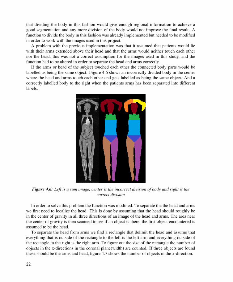
A problem with the previous implementation was that it assumed that patients would liewith their arms extended above their head and that the arms would neither touch each othernor the head, this was not a correct assumption for the images used in this study, and thefunction had to be altered in order to separate the head and arms correctly.

If the arms or head of the subject touched each other the connected body parts would belabelled as being the same object. Figure 4.6 shows an incorrectly divided body in the centerwhere the head and arms touch each other and gets labelled as being the same object. And acorrectly labelled body to the right when the patients arms has been separated into differentlabels.

Figure 4.6: Left is a sum image, center is the incorrect division of body and right is thecorrect division

In order to solve this problem the function was modified. To separate the the head and armswe first need to localize the head. This is done by assuming that the head should roughly bein the center of gravity in all three directions of an image of the head and arms. The area nearthe center of gravity is then scanned to see if an object is there, the first object encountered isassumed to be the head.

To separate the head from arms we find a rectangle that delimit the head and assume thateverything that is outside of the rectangle to the left is the left arm and everything outside ofthe rectangle to the right is the right arm. To figure out the size of the rectangle the number ofobjects in the x-directions in the coronal plane(width) are counted. If three objects are foundthese should be the arms and head, figure 4.7 shows the number of objects in the x-direction.

22

In order to find the height of the head the image is scanned line wise from left to right andthe amount of large(more than a couple of pixels wide) objects are counted. If there are threeobjects encountered these should be the head and the arms. The height is recorded in orderto know where the head starts and ends in the y-direction. The width of the head is found bytaking the widest area of the middle of the three objects.

Figure 4.7: An image of arms and head. The numbers on the right indicate the number ofconnected objects in x direction (coronal view)

4.6.2 Segmenting each body partThis section describes how the segmentation works for each body part. This segmentationsegments the right and left arm the same way, the same goes for the right and left leg.

Arms, collarbones and shoulder bladesThe arms have 6 different bones, radius, ulna and humerus on both the left and right arm,all of them should be visible assuming that the images does not have any major artefacts inthem. It is also possible to segment the collarbones (clavicle) and some of the shoulder blades(scapulae). Because the bones are easily visible the segmentation procedure is simple, it goesas follows:

1. Mask out everything that is not part of the arms or upper torso from the sum image

2. Extract the voxels that have a low intensity value in the sum image

3. Remove objects that are smaller than a certain number of voxels

Figure 4.8 shows an example segmentation of the arms and shoulders.

Head There are two things in the head that will have a low intensity value in the head onfat-water MRI images, these are bone and air. Separating these from each other can be quitedifficult since the air can be in a close proximity to the bones, so a function to segment thetrachea was needed. The head segmentation function works the following way:

1. Mask out everything in the sum image that is not part of the head

23

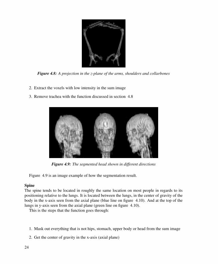
Figure 4.8: A projection in the z-plane of the arms, shoulders and collarbones

2. Extract the voxels with low intensity in the sum image

3. Remove trachea with the function discussed in section 4.8

Figure 4.9: The segmented head shown in different directions

Figure 4.9 is an image example of how the segmentation result.

SpineThe spine tends to be located in roughly the same location on most people in regards to itspositioning relative to the lungs. It is located between the lungs, in the center of gravity of thebody in the x-axis seen from the axial plane (blue line on figure 4.10). And at the top of thelungs in y-axis seen from the axial plane (green line on figure 4.10).

This is the steps that the function goes through:

1. Mask out everything that is not hips, stomach, upper body or head from the sum image

2. Get the center of gravity in the x-axis (axial plane)

24

Figure 4.10: A schematic of the lungs and spine in black color. The Green line is the top ofthe lungs in y-axis (axial plane) and the blue line is the center of gravity in x-axis (axial

plane). The red square is where the function looks for the spine

3. Find the top of the lungs in y-axis in every slice of the image (axial plane)

4. Look in a small squared area that is located around the locations gathered from the twoprevious steps, get everything that has a low intensity value, this is usually the spine, butsometimes also the lungs

5. Mask out lungs

PelvisA problem with the body division is that the pelvis is actually larger than the label assignedto be the pelvis area. Because of this the lower part of the stomach and the upper part of thelegs need to be included in the pelvis segmentation in order to get a correct segmentation ofthe pelvis. Figure 4.11 below shows how parts of the pelvis extends into the stomach and legregions.

1. Remove everything from the sum image that is not part of the pelvis region, the lower 20percent of the stomach and the upper 20 percent of the legs.

2. Threshold the lower intensity values in the sum image

3. Remove the intestines from the sum image with the function discussed in section 4.8

4. Remove all small objects (that are too small to be part of the pelvis)

LegsThe leg segmentation is fairly simple and consists of looking at the legs and to threshold everyobject that has a low intensity values, then you take out the largest objects. The largest objectsfrom those with a low intensity values should be the 6 major leg bones namely, femur, tibiaand fibula on the left and right side.

25

Figure 4.11: An image of a pelvis extending into the nearby regions

Figure 4.12: Example of the result from segmenting the bones in the legs(and partially hip)shown from three different angles

26

4.7 Segmentation method2 - FilterThe following seciton describes the second segmentation method that was implemented.

4.7.1 Filter ideaCertain anatomical patterns are common in the proximity of bones. In order to increase thelikelihood that the segmented voxels are bone a filter can be constructed that detects thesepatterns. The filter was constructed based on the idea that bone contains bone marrow and issurrounded by muscle. There are bones in the human body that does not follow this patternsince they contain little bone marrow or is not surrounded by muscle, but a large portion of thebones does follow this pattern. Figure 4.13 shows an example of a bone that has bone marrowin the center and muscle on the other side.

Figure 4.13: An image showing muscle, bone and bone marrow in the fat(left) andwater(right) images

Bone marrow contains a high concentration of fat, and will thus have a high intensity inthe fat image. Muscle on the other hand has a high concentration of water. Bone has a lowconcentration of both water and fat, and will thus give a weak signal in both the fat and waterimages. Table 4.2 displays these relationships.

Muscle Bone Bone marrow

Water image high low low

Fat image low low high

Table 4.2: Predicted intensities in different tissue types in the water and fat image. In orderfor the filter to be viable these predictions should be accurate

27

The filter was constructed to find patterns in the images where there is low concentration ofboth water and fat in the middle, a high concentration of fat on one side, and a high concentra-tion of water on the other. This is supposed to represent a bone with bone marrow on one sideand muscle on the other.

In order to verify that the pattern is indeed present, bone, the inside of bone and the arearight outside of bone was measured in order to see if their intensity values corresponded withwhat was expected. If the assumption is correct the measured values should have the samepattern as described in table 4.2. The measured values can be seen below in table 4.3.

Muscle Bone Bone marrow

Water image 537.8 190.9 54.2

Fat image 61.2 114.6 631.3

Table 4.3: Measured intensity values in different tissue types around skeleton

It is evident that the measured values follow the expected pattern.

4.7.2 DescriptionThe function starts by creating an integer probability map of every voxel being bone, in thismap every voxel in the image corresponds to a probability. Initially every entry in the proba-bility map is set to 0. The main portion of the function, described below, focuses on findingvoxels that are believed to be bone and increasing the integer value of that point in the proba-bility map.

The filter function goes through the image in x, y, and z-directions and search for voxelswith low intensity in both the water and fat image, these are candidates for being bone. Theneach side of those candidate voxels are investigated, if one side has a high intensity in thewater image and the opposite side has a high intensity in the fat image the probability ofthe candidate voxel being bone is increased in the probability map. The algorithm does thisprocess repeatedly in all three directions(x, y, z) of the image in order to find bones that arepointing in different directions.

To find bones of varying thickness the number of voxels that are investigated on each sideof the candidate voxel varies, the number of voxels searched is called the window size. Theoptimal result found was achieved when every window size between 2 and 6 was used. Aver-aging(mean) was used to determine if the voxels in the window were deemed to have a highintensity or not.

When the filter function has been run in every direction, with every window size the voxelswith the highest probability is extracted.

Below is pseudo code that describes how the filter works.procedure Filter()

1: Set probability map to 0 for all voxels

28

Figure 4.14: Schematic of muscle, bone and bone marrow. Also shows an example window

2: for Every window size do3: for For every direction (x, y and z) do4: for Voxel with low intensity in both images do5: if high intensity in fat image on one side and high intensity in water image on

opposite side then6: Increase likelihood of the voxel being bone in probability map7: end if8: end for9: end for

10: end for11: Threshold probability map for voxels with high probability.

4.7.3 Determining parametersThe filter function has several different input parameters and work had to be done to find outwhich parameters were the optimal. Some of the parameters that had to be chosen includedwindow sizes, what threshold should be used when thresholding the probability map and howmuch the lung mask needed to be dilated.

One of the most important things that had to be decided was which intensity values shouldbe considered as muscle, bone and bone-marrow. The process of determining this was aniterative process which got increasingly better as the project went along.

Values were initially chosen manually and by using ROIs of the different types of tissues.ROIs were placed in areas that contained muscle, bone and bone marrow in different imagesand the intensity in the ROIs were measured. The knowledge from the ROIs gave some knowl-edge of what values were appropriate thresholds. This method was not very effective however

29

as it assumes that only homogeneous regions will be inside of the filter window, in reality thefilter can often encounter many different types of tissues.

Reference segmentations were created for the second iteration, these reference segmenta-tions could be compared to the result from the filter function. If a parameter was changed thenthe dice coefficient between the reference and automatic result could be determined and it waspossible to see whether the new threshold gave a higher dice coefficient than the last. Thisis a naïve approach that can get stuck in local maximums, but the result form the ROIs andthe manual changing of parameters had given some indication of what the optimal thresholdswere. This was also the method that was used to determine the other parameters like windowsize. The faulty assumption in this approach is that there is no set of thresholds that is optimalfor all MRI images, each image needs its own set of intensity thresholds.

The third iteration tried to solve the problem of every image needing its own set of thresh-olds. This was done by using Otsu’s method [13]. Otsu’s method finds the threshold levelwhere the intra-class variance between the object and the background is minimal. Otsu’smethod did however underestimate the threshold levels so they had to be multiplied by a valuedetermined using the method in iteration two. This was the final method that were implementedto chose thresholds.

4.8 Post-processingAfter the two segmentation algorithms had been implemented certain areas suffered from oversegmentation, most significantly intestines and the trachea would often get segmented as beingskeleton. Functions were thus created to try to remove those areas after the normal segmenta-tion functions were finished. A new body mask was also implemented as the old one was notwell suited for this project, and would often overestimate the size of the body.

4.8.1 Body maskThe problem with the body mask was that it often overestimated the size of the body, becauseof that some areas that were air would get segmented as bone. One particular area like thatwas the air between the arms and the head which is shown in the image below. Figure 4.15shows how the old body mask overestimates the size of the body and because of that the headand arms are connected to each other.

A new function was developed to fix this problem. The way the function worked is describedbelow.

1. Threshold the sum image (threshold decided by otsus method)

2. Do a morphological close of the image

3. Fill in holes in 3D

4. Extract largest object (this is the body)

30

Figure 4.15: An image showcasing how the old method would overestimate the size of thebody

Figure 4.16: The steps taken when creating the new body mask

Figure 4.16 shows the steps taken when creating the body mask.This new body mask is not perfect since it can sometimes underestimate the volume of the

body instead, but since bone is most often deep in the body this has not caused any majorproblems for this project.

4.8.2 Intestine maskAn intestine mask was needed in order to be able to remove the intestines from the skeletalsegmentations in the post-processing section of the functions. The intestine mask tries finds allthe areas in the abdomen that have a low intensity in both water and fat image that are not partof the hip. A function to locate the femoral heads was already implemented, so the intestinefunction uses that knowledge to approximate the location of the hip. The function assumes thatthe highest tip of the pelvis in the y-direction(sagittal view) is a certain number of voxel abovethe femoral head, experimentation gave an appropriate y-coordinate that removes most of theintestines while not removing any of the hip in the pelvis area. The function then removes allsmall objects as the intestines tends to be a long connected object, this can remove any smallarea of the pelvis that might wrongfully be segmented as intestines.

4.8.3 Trachea maskThe trachea was found using a virtually the same method that was used to find the spinementioned in section 4.6.2, but the trachea function looks at the bottom of the lungs in y-

31

direction (axial plane) instead of at the top. The trachea is located between the lungs, so thefunction initially measures where the lungs start and end in x-direction(axial plane) and createsa square in between both lungs where the trachea is expected to be found. Every voxel witha low value in the sum image and that is inside the square is extracted. The lungs are thenmasked out as they can be included in the trachea mask.

32

5. Result

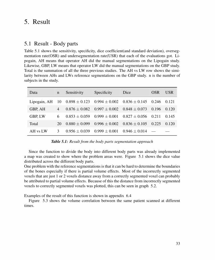
5.1 Result - Body partsTable 5.1 shows the sensitivity, specificity, dice coefficient(and standard deviation), overseg-mentation rate(OSR) and undersegmentation rate(USR) that each of the evaluations got. Li-pogain, AH means that operator AH did the manual segmentations on the Lipogain study.Likewise, GBP, LW means that operator LW did the manual segmentations on the GBP study.Total is the summation of all the three previous studies. The AH vs LW row shows the simi-larity between AHs and LWs reference segmentations on the GBP study. n is the number ofsubjects in the study.

Data n Sensitivity Specificity Dice OSR USR

Lipogain, AH 10 0.898 ± 0.123 0.994 ± 0.002 0.836 ± 0.145 0.246 0.121

GBP, AH 4 0.876 ± 0.082 0.997 ± 0.002 0.848 ± 0.073 0.196 0.120

GBP, LW 6 0.853 ± 0.059 0.999 ± 0.001 0.827 ± 0.056 0.211 0.145

Total 20 0.880 ± 0.099 0.996 ± 0.002 0.836 ± 0.105 0.225 0.120

AH vs LW 3 0.956 ± 0.039 0.999 ± 0.001 0.946 ± 0.014 — —

Table 5.1: Result from the body parts segmentation approach

Since the function to divide the body into different body parts was already implementeda map was created to show where the problem areas were. Figure 5.1 shows the dice valuedistributed across the different body parts.One problem with the reference segmentations is that it can be hard to determine the boundariesof the bones especially if there is partial volume effects. Most of the incorrectly segmentedvoxels that are just 1 or 2 voxels distance away from a correctly segmented voxel can probablybe attributed to partial volume effects. Because of this the distance from incorrectly segmentedvoxels to correctly segmented voxels was plotted, this can be seen in graph 5.2.

Examples of the result of this function is shown in appendix 6.4Figure 5.3 shows the volume correlation between the same patient scanned at different

times.

33

Figure 5.1: A map showing the dice coefficients in different body parts

Figure 5.2: A plot of incorrectly segmented voxels and their distance to a bone voxel in thereference segmentation

34

Figure 5.3: The skeleton volume from two scans of the same person at different times

35

5.2 Result - FilterThis segmentation function was evaluated with the same methods used to evaluate the firstsegmentation function, namely the overlap between the manually segmented skeleton and theautomatically segmented by this function. Evaluation was done on the same images used forthe first function, thus making the comparison between the two functions easier.

Data n Sensitivity Specificity Dice OSR USR

Lipogain, AH 10 0.953 ± 0.025 0.999 ± 0.001 0.949 ± 0.139 0.054 0.047

GBP, AH 4 0.973 ± 0.009 0.999 ± 0.001 0.963 ± 0.018 0.026 0.046

GBP, LW 6 0.908 ± 0.042 0.999 ± 0.001 0.918 ± 0.032 0.071 0.092

Total 20 0.941 ± 0.026 0.999 ± 0.001 0.944 ± 0.083 0.053 0.059

AH vs LW 3 0.956 ± 0.009 0.999 ± 0.001 0.946 ± 0.014 — —

Table 5.2: Result from the filter segmentation approach

Partial volume artefacts are artefacts that can arise in MRI imaging because the MRI scannerdoes not have a resolution that is high enough to image small objects or objects to the borderof other objects. Because of partial volume effects objects can get very blurry lines at theedges. To figure out how much partial volume effects might have affected the result a plot wasmade of how far away incorrectly segmented voxels were to correctly segmented voxels. Ifthey are just one voxel away from a correctly segmented voxel the chance that those voxels areincorrectly segmented as a result of partial volume effects is high.

Another important aspect is how well this method can be used to estimate bone volume.Measuring bone volume could be of help to identify and diagnose osteoporosis. To figureout how consistently this method measured bone volume we analysed patients that had beenscanned twice and checked how well the bone volume correlated in both scans. 39 test sub-jects had been scanned twice and were evaluated. Figure 5.6 is a scatter plot of the relationshipbetween the amount of bone segmented by this method in scans done on the same person atdifferent times. The correlation between the the amount of bone voxels in the first and secondscan was 0.9402.

Examples of the result of this function is shown in appendix 6.4

36

Figure 5.4: Dice coefficients divided into different body parts for the filter function

Figure 5.5: A map of incorrectly segmented voxels and their distance to bone for the filterfunction

37

Figure 5.6: x-axis shows the first time scanned in number of voxels determined as bone,y-axis shows the second scan also in number of voxels

38

6. Discussion and conclusion

From table 5.1 and 5.2 it is evident that specificity is much higher than sensitivity, this is notsurprising considering the fact that there is more non-bone voxels in the image than there arebone voxels. Both functions appear to have a similar dice coefficients in both the Lipogain andGBP study, this can indicate that a patients BMI does not have a large impact on the result ofthe segmentations. There does on the other hand appear to be a difference between the twooperators, the study by LW gets lower dice scores than the ones done by AH with both thefilter and the body part method. A certain degree of inter operator variation is to be expected.The Lipogain study seems to have a higher standard deviation in dice score than than the GBPstudy, it could be a result of too small sample size or because of the fact that there is a biggerdifference in dice score in the Lipogain study.

Measuring the stability created some difficulty in this project since it was not possible to domany manual segmentations in the limited time span. The stability was measured by lookingat the standard deviation of the dice coefficients and repeatability was tested by segmentingthe same person from two different scans and measuring how similar the bone volume wasbetween each scan.

The computational times were not evaluated exactly on either function, this is because of thefact that the computational speeds of both functions vary depending on whether certain imagesthe functions needs have been created previously or not. The body part function for instancerequires the image of the body divided into 8 parts and the filter function needs a lung mask.If these images have been created prior to running the functions, the functions run faster. Thecomputational speeds were roughly calculated though, and both functions takes around oneminute to segment a 256x252x184 voxel large image.

It should be noted that all the images used in this thesis were collected with the same settingsin the MRI machine, and they were only collected on 1.5Tesla machines. This makes it hard toknow exactly how the functions will work on different images, especially if they are collectedon MRI machines with different field strength magnets.

6.1 Discussion - Body parts methodIt is hard to say how well this function works as I was unable to find any other papers onfull body skeletal segmentation, but the dice score of 0.836 (as seen in table 5.1) can be anindicator of how well the function works. The over and under segmentation rates were fairlyhigh (0.2250 and 0.1202 respectively), which shows that both over and under segmentation isa large problem for this function.

Graph 5.2 shows that a majority of the voxels that are incorrectly segmented are at a distanceof only one voxel away from a correctly segmented voxel, so a large portion of these voxelscould probably be attributed to partial volume effects.

Image 5.1 show that the legs have the highest dice coefficient, this is not surprising as thelegs consists of large bones that have simple straight shapes. The stomach, upper body and

39

pelvis on the other hand gets lower dice values. This is not especially strange either as thoseareas have many small bones, bones with varying intensity values and complex shapes (thepelvis for instance). The stomach and pelvis also have intestines, which is a problem with themethod.

Figure 5.3 is a good indicator of stability as it shows the amount of pixels segmented as bonein the same person at two different scan times. Since a person will probably not loose muchbone mass within the short period of time between the scans, the amount of bone segmentedshould be virtually the same on both occasions. Since one subject had roughly 86000 voxelssegmented as bone in the first scan and 66000 on the second it is clear that this function is notstable enough to calculate bone mass. A contributing factor to this instability could be that thepatella (kneecap) does not always get segmented as bone with this function. A future revisionof the function should probably try to fix that. The spine segmentation is most likely not verystable either as it assumes that the spine will be roughly within the same position on everysubject, because of that the function will probably work poorly on subjects with scoliosis.

The current implementation of this method still has several major issues that should beresolved in order for this to be a good solution. One problem is intestines, which often getsclassified as bone in the pelvic area since it has a close proximity to the pelvic bone. Creatinga better mask of the intestines could greatly reduce this problem, but this was not implementedsince time was limited.

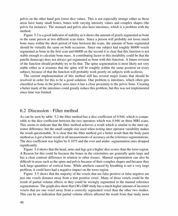
6.2 Discussion - Filter methodAs can be seen by table 5.2 the filter method has a dice coefficient of 0.944, which is compa-rable to the dice coefficient between the two operators which was 0.946 on three MRI scans.This seems to indicate that the filter method achieves a result which is similar to the inter op-erator difference, but the small sample size used when testing inter operator variability makesthe result questionable. It is clear that the filter method got a better result than the body partsmethod as it got a better result in all measurements of accuracy on the reference segmentations.The dice coefficient was higher by 0.1075 and the over and under- segmentation rates droppedsignificantly.

Figure 5.4 shows that the head, arms and legs got a higher dice scores than the torso region.A Reason for this could be because the bones in the extremities are generally quite large andhas a clear contrast difference in relation to other tissues. Manual segmentation can also bedifficult in areas such as the spine and pelvis because of their complex shapes and because theylack large quantities of cortical bone. While artefacts caused by breathing is not a very largeproblem, it could have had a negative impact on the torso region.

Figure 5.5 shows that the majority of the voxels that are false positive or false negative arejust one voxels distance away from a true positive voxel. Many of those voxels could be theresult of partial volume effects or they could be wrongly segmented in the manual referencesegmentation. The graph also show that LWs GBP study has a much higher amount of incorrectvoxels that are one voxel away from a correctly segmented voxel than the other two studies.This can be an indication that partial volume effects affected the result from that study more

40

than the other two studies, and it could explain why the results from that study were not asgood as the result from the other two.

A problem with the implementation of this function is that it only checks for bone in purex-, y- or z-axis, it does not check in any other angle. So the function could have a hard timeto locate bone which is not aligned with either of those directions. The reason for this is tokeep the function simple and fast, looking for bones in other directions would complicate thefunction and speed up the computational time.

As stated earlier, there are anatomical patterns other than bone that can be detected by thefilter, this is because the pattern can be found in areas other than bones. There are also partsof the skeletal system that wont be found by this filter since the bones might not contain bonemarrow, or they might not lie close to muscle. Voxels that are found although they are not boneare considered over segmentation and voxels that are not found are under segmentation. Thepost-processing that was done tried to reduce the over segmentation as much as possible, butover segmentation problems still exist. Most of the over segmentation that is still present afterpost-processing is intestines in the stomach and pelvic area.

Table 5.2 show that the under segmentation rate is 0.059 and over segmentation rate is0.053, this is a large improvement over the body parts function which had more than twice ashigh under segmentation rate and four times as high over segmentation rate

One way in which the stability can be measured is by looking at the standard deviation ofthe dice coefficient. For the 20 MRI scans used to evaluate this method the standard devia-tion for dice was 0.083 on average. There did seem to be quite a large difference betweenthe different image series used to evaluate this function though, with a standard deviation of0.1398 when AH segmented the images in the Lipogain study, but only 0.0184 for the imagesAH segmented in the GBP study. It is difficult to say why this difference might be there, butit may be because there was only 4 images used from the GBP study. It could possibly alsobe because of the fact that the patients in the in GBP study had a much higher BMI than thepatients in the Lipogain study.

Figure 5.6 shows the repeatability of the function. A correlation coefficient of 0.9402would probably not be able to accurately diagnose osteoporosis but could possibly be used asan indicator of the disease. It should be noted that it was not investigated whether or not thebone volume measured with this function was close to the real bone volume of the patients,just whether they were consistent across different scans of the same person.

A problem with this method was that it was sensitive to image artefacts, this was especiallyclear on the larger test subjects where the field of view was sometimes to small to get a goodimage of the whole person.

6.3 ConclusionAs magnetic resonance imaging increases in popularity more segmentation techniques areneeded in order to analyse the images they produce. New medical imaging systems ofteninclude methods for registration and segmentation of many different body parts, and using the

41

skeletal system could help to localise other structures and organs in the body. Segmentationof skeleton in MRI is still not very widespread and not much has been published about it, somore research is needed. Techniques like these could help research on skeletal and cartilagedisorders that often lack automatic methods for analysing skeletal deterioration.

This paper has shown that it is possible to do skeletal segmentation with relatively simpleand fast methods that does not rely on a deformable model or atlas.

Unfortunately these methods could not be compared to other skeletal segmentation meth-ods since no papers on full body MRI skeletal segmentation were found, but methods usingdeformable models would most likely yield a better segmentation result but take a longer timeto execute.

Both methods proved to be robust enough to be able to be used on both high and low BMIpatients, and achieved roughly the same precision regardless of which of the two image seriesthey were tested on. It would however be good to test the methods on MRI scanners withdifferent magnetic field strengths since both of the image series used here were taken on 1.5Tesla machines. The dice score is a good indicator of how well the segmentation works andsince the filter function got a significantly higher dice score than the body parts function, it ismost likely the better option for segmenting skeleton.

Whether or not these segmentation methods achieve an acceptable result depends on whatthey are going to be used for. These methods will most likely achieve results that are goodenough to be able to help with registration of whole-body images and could be used to assistother segmentation methods, but neither of the methods presented in this paper are accurateenough that a good estimate of bone volume is possible, thus measuring osteoporosis andsimilar disorders will most likely require more complex methods.

There is still some problems that these methods do no handle very well, and over segmen-tation is still a problem that needs to be solved if bone volume is to be measured or if a highlyaccurate method is needed.

Platinum proved to be a useful image analysis platform to do this work on since it has alarge amount of image analysis tools already implemented.

6.4 Suggestions for future workThere are multiple ways in which the work done in this thesis could be improved, the mostnotable of them are mentioned in this section.

A way in which this work could be improved is to combine the filter and body parts seg-mentation methods in order to utilize the strength from both methods, that way you could getthe accuracy of the filter and use the prior knowledge of the human body that the body partsmethod uses. Another way in which prior knowledge could help segmentation would be totry to label the bones found by the filter function, this would also be useful to help locate andsegment other organs and parts of the body.

The functions developed in this thesis could also be used as starting points in machinelearning or deformable model algorithms, since these functions are quite fast ( 1min) thatcould save time and increase accuracy for more advanced algorithms.

42

Since neither of the two functions developed here tries to segment the ribs, that could be anext step in a future revision of the functions. In order to segment the ribs you would mostlikely need images with higher resolution or you would need to use prior knowledge of thelocation of the ribs since the ribs are difficult to see even for a human observer.

It would have been good to evaluate these functions on a larger number of MRI images,specifically images with different settings on the MRI scanners, with different intensity cor-rections and on MRI scanners with higher field strength magnets. Testing the methods on MRIscanners with stronger magnets would have been useful as 3 Tesla scanners are starting tobecome more prominent and it could show the robustness of the algorithms.

The post-processing used in this thesis could been improved. The intestine mask developedin this thesis is not accurate enough to get all the intestines, this is partially because of the factthat the intestines can have an intensity very similar to bone and be very close to the pelvis.Other types of post-processing functions would probably also increase the accuracy and qual-ity of the segmentations.

The body parts segmentation method has several problems which decreases its performance,for instance the function does not always segment the patella (kneecaps) of the subjects andthe stability of the spine function could be greatly improved since the spine function largelyrelies on the position of the lungs to locate the spine. If the spine function used several organsto locate the lungs the reliability could be improved.

A problem with the filter function is that it only checks for bone in a pure x-, y- or z-axisand does not look at any other angles. Making the function look in more directions wouldincrease the accuracy and reliability of the function, but would have a negative effect on thespeed of the function and would make the function more complicated. The filter function alsouse the mean value of the filter window to determine what type of tissue is inside the window,this might not be the optimal choice. Trying other metrics for determining tissue type couldresult in a better result.

43

References

[1] Image segmentation at Wikipedia. http://en.wikipedia.org/wiki/Image_segmentation,2013. [Online; accessed 14-August-2013].

[2] Platinum. https://code.google.com/p/platinum-image, 2013. [Online; accessed13-August-2013].

[3] D. Cobzas, N. Birkbeck, M. Schmidt, M. Jagersand, and A. Murtha. 3d variational brain tumorsegmentation using a high dimensional feature set. In Computer Vision, 2007. ICCV 2007. IEEE11th International Conference on, pages pp.1–8, Rio de Janeiro, Brazil, October 2007.

[4] B. Gilles and N Magnenat-Thalmann. Musculoskeletal mri segmentation using multi-resolutionsimplex meshes with medial representations. Medical Image Analysis, Vol. 14:pp.291–302, 2010.

[5] KH. Höhne and WA. Hanson. Interactive 3d segmentation of mri and ct volumes usingmorphological operations. Journal of Computer Assisted Tomography, Vol. 16(2):pp.285–294,1992.

[6] MR. Kaus, J. von Berg, J. Weese, W. Niessen, and Pekar V. Automated segmentation of the leftventricle in cardiac mri. Medical Image Analysis, 8(3):245 – 254, 2004. Medical ImageComputing and Computer-Assisted Intervention - MICCAI 2003.

[7] A. Kelemen, G. Szekely, and G. Gerig. Three-dimensional model-based segmentation of brainmri. In Biomedical Image Analysis, Proceedings. Workshop on, pages pp.4–16, Santa Barbara,CA, USA, June 1998.

[8] A. Kikuchi, M. Onoguchi, H. Horikoshi, K. Sjöstrand, and L. Edenbrandt. Automatedsegmentation of the skeleton in whole-body bone scans: influence of difference in atlas. NuclearMedicine Communications, Vol. 33(9):pp.947–953, 2012.

[9] H. Lamecker, M. Seebaß, H.C. Hege, and P. Deuflhard. A 3d statistical shape model of the pelvicbone for segmentation. In In: Proc. of the SPIE, vol. 5370, pages pp.1341–1351, Rio de Janeiro,Brazil, 2004.

[10] G.P. Mazzara, R.P. Velthuizen, J.L. Pearlman, H.M. Greenberg, and H. Wagner. Brain tumortarget volume determination for radiation treatment planning through automated mrisegmentation. International Journal of Radiation Oncology*Biology*Physics, 59(1):300 – 312,2004.

[11] A. Mitiche and J.K. Aggarwal. Image segmentation by conventional and information-integratingtechniques: A synopsis. Image and Vision Computing, Vol. 3(2):pp.50–62, 1985.

[12] N. Moon, E. Bullitt, K. van Leemput, and G. Gerig. Model-based brain and tumor segmentation.In Pattern Recognition, 2002. Proceedings. 16th International Conference on, volume Vol. 1,pages pp.528–531, October 2002.

[13] N. Otsu. A threshold selection method from gray-level histograms. IEEE Trans. Systems, Manand Cybernetics, Vol. 9:pp.62–66, 1979.

44

[14] J. Sjölund et al. A machine learning approach for automatic segmentation of bone in t1-weightedmri. Procedings of the SSBA, 2013.

[15] R. Smith-Bindman, D.L. Miglioretti, and E.B. Larson. Rising use of diagnostic medical imagingin a large integrated health system. Health Aff (Millwood), Vol. 27:pp.1491–1502, 2008.

[16] W.M. Wells, W.E.L. Grimson, R. Kikinis, and F.A. Jolesz. Adaptive segmentation of mri data.Medical Imaging, IEEE Transactions on, Vol. 15(4):pp.429–442, 1996.

45

Appendix

Body Parts Segmentation ResultsHere is some images of the body parts segmentation function, the one described in chapter 4.6

Figure 6.1: Left: Z-projected skeleton, Right: 3D skeleton seen from three different angles

46

Figure 6.2: Left: Z-projected skeleton, Right: 3D skeleton seen from three different angles

Figure 6.3: Left: Z-projected skeleton, Right: 3D skeleton seen from three different angles

47

Filter Segmentation ResultsHere is examples images of the filter segmentation function, described in chapter 4.7

Figure 6.4: Left: Z-projected skeleton, Right: 3D skeleton seen from three different angles

48

Figure 6.5: Left: Z-projected skeleton, Right: 3D skeleton seen from three different angles

Figure 6.6: Left: Z-projected skeleton, Right: 3D skeleton seen from three different angles

49