automatic reduction of pdes defined on domains with...

MATHICSE

Mathematics Institute of Computational Science and Engineering

School of Basic Sciences - Section of Mathematics

EPFL - SB - MATHICSE (Bâtiment MA) Station 8 - CH-1015 - Lausanne - Switzerland

http://mathicse.epfl.ch

Address:

Phone: +41 21 69 37648

Automatic reduction of PDEs

defined on domains with variable shape

Andrea Manzoni, Federico Negri

MATHICSE Technical Report Nr. 19 .2016

June 2016

http://mathicse.epfl.ch/

Automatic reduction of PDEs defined ondomains with variable shape

Andrea Manzoni and Federico Negri

Abstract In this work we propose a new, general and computationally cheap way totackle parametrized PDEs defined on domains with variable shape when relying onthe reduced basis method. We easily describe a domain by boundary parametriza-tions, and obtain domain deformations by solving a solid extension through a linearelasticity problem. The procedure is built over a two-stages reduction: (i) first, weconstruct a reduced basis approximation for the mesh motion problem; (ii) then,we generate a reduced basis approximation of the state problem, relying on fi-nite element snapshots evaluated over a set of reduced deformed configurations.A Galerkin-POD method is employed to construct both the reduced problems, al-though this choice is not restrictive. To deal with unavoidable non affinities aris-ing in both cases, we apply a matrix version of the discrete empirical interpolationmethod, allowing to treat geometrical deformations in a non-intrusive, efficient andpurely algebraic way. In order to assess the numerical performances of the proposedtechnique we consider the solution of a parametrized (direct) Helmholtz scatteringproblem where the parameters describe both the shape of the obstacle and otherrelevant physical features.

1 Introduction

The reduced basis (RB) method provides nowadays a very efficient approach for thenumerical approximation of problems arising e.g. from engineering and applied sci-ences which require the repeated solution of differential equations. Well-known in-stances include partial differential equations (PDEs) depending on several parame-ters, PDE-constrained optimization, as well as optimal control and design problems.

A. Manzoni · F. NegriCMCS-MATHICSE-SB, Ecole Polytechnique Federale de Lausanne,Station 8, CH-1015 Lausanne, Switzerlande-mail: [email protected],[email protected]

1

[email protected],[email protected]

2 Andrea Manzoni and Federico Negri

In all these cases, the RB method replaces the original large-scale numerical prob-lem (or high-fidelity approximation) originated by applying, e.g., a finite element(FE) method, with a reduced problem of substantially smaller dimension [25, 14].

In all these contexts, relevant instances of parametrized PDEs arise when dealingwith problems defined over spatial domains undergoing geometrical transforma-tions; this is the case of design problems, where being able to rapidly adapt existingmeshes to design variations is essential to perform, e.g., shape optimization in anefficient way.

On the other hand, an offline/online stratagem, relying on the so-called affineparametric dependence, is required to gain a strong computational speedup whendealing with RB approximations to parametrized PDEs. In this respect, dealing withshape variations has often a major impact on the computational efficiency, since:

1. equipping the set of varying shape with a suitable parametrization is an in-volved, highly problem-dependent, task. In the RB context, parametric mapsdefined over the whole domain are needed to formulate the PDE problem ona parameter-independent reference configuration. However, in computed-aideddesign (CAD), boundary parametrizations under analytic form are usually de-fined for surfaces (in d = 3 dimensions) or curves (d = 2), rather than for thewhole domain, thus preventing their direct use within the RB context;

2. geometrical parametrizations usually yield nonaffine parametric dependencies,so that an affine approximation of PDE operators has to be recovered throughthe empirical interpolation method (EIM) [3, 19] – or its discrete counterpart(DEIM) [6]. This usually entails an extensive work on the continuous formulationof the problem, as well as intrusive changes to its high-fidelity implementation.

Several techniques have been exploited to perform RB approximations of PDEsdefined on varying domains. The simplest idea is to rely on affine maps, whichautomatically induce an affine parametric dependence, but only enable elementarydeformations [26].

More involved deformations can be obtained by introducing nonaffine mapsyielding volume-based parametrizations. Within this class, we mention free-formdeformations (FFD) [18, 27, 21, 2] and interpolation relying on radial basis func-tions (RBF) [20, 23, 8, 10] as remarkable instances. Both techniques originate globaldeformations by combining the displacements of a set of control points. FFD dealwith a cartesian lattice of control points and a tensor product of splines to combinecontrol points displacements; these latter are instead interpolated in the RBF case,where the control points can be freely located inside the domain. In both cases,however, selecting the number of control points, their position and admissible dis-placements is far from being trivial.

Another option relies instead on the use of transfinite mappings, which definethe interior points of the original domain as linear combinations of points on theboundaries [11]. In particular, each edge of the original domain is obtained as aone-to-one mapping of the corresponding edge on the reference domain, through avector of geometrical parameters, see e.g. [9, 15, 16].

Automatic reduction of PDEs defined on domains with variable shape 3

Finally, isogeometric analysis has been recently exploited in [22] as a possi-ble way to deal with parametrized profiles with respect to parameters (such as theNACA number in the case of flows past airfoils) of simple interpretation.

The mesh motion strategy considered in this work allows to simplify the way todeal with geometrical deformations, by relying on (i) simple boundary parametriza-tions, and (ii) the solution of a solid extension problem. Moreover, we exploit arecently proposed matrix version of DEIM (MDEIM, [23, 35, 5]) to perform in-expensive evaluations of the online matrix operators for both the deformation andthe state problem. Hence, we first recover an affine parametric dependence in thehigh-fidelity arrays appearing in both problems, by applying MDEIM and DEIMfor matrix and vector operators, respectively. This is performed in a purely alge-braic, black-box, in order to overcome the application of the EIM on the continuousformulation of the problem, which is usually highly demanding, see e.g. [12, 24, 4].Then, we perform the RB approximation of both the deformation and the state prob-lem, relying on a Galerkin-POD technique.

The paper is structured as follows. In Sect. 2 we describe the proposed meshdeformation technique. In Sect. 3 we introduce the class of problems we deal within this work, as well as the main features of the RB approximation framework wedevelop. The whole computational procedure is then applied in Sect. 4 for the sakeof the efficient solution of a parametrized (direct) Helmholtz scattering problem.Finally, some conclusions are reported in Sect. 5.

2 Solid extension mesh moving techniques

Let Ω ⊂ Rd be a spatial domain with boundary Γ , where d = 2,3 is the number ofspace dimensions. We denote by Γh a discretization of the boundary Γ and by Ωh avolumetric mesh of that geometry, e.g. a triangular mesh in 2D or a tetrahedral meshin 3D. Given a boundary deformation Γh 7→ Γh, mesh deformation techniques adaptthe mesh Ωh such that (i) the updated mesh Ωh conforms to the updated boundary,i.e. ∂Ωh = Γh and (ii) the geometric embedding of Ωh (i.e., its nodes positions) ismodified while keeping fixed the mesh topology (i.e., its connectivity).

Among a wide range of existing mesh deformation techniques, here we focuson the so called mesh-based variational methods (see, e.g., [30]). These latter com-pute smooth harmonic [1], biharmonic [13] or elastic [33, 32, 31] deformations bysolving Laplacian, bi-Laplacian or elasticity problems, respectively. Specifically, weconsider this latter, which is often referred to as solid-extension mesh moving tech-nique (SEMMT) [33, 32, 31].

Before describing the method, let us first introduce a non-overlapping decompo-sition of the boundary Γ into a deformable portion γ and a fixed one ∂Ω \ γ . Given aboundary displacement hhh ∈ [H1/2(γ)]d such that γ = x ∈Rd : x = x+hhh, x ∈ Ω,the SEMMT generates a deformed domain Ω as

Ω(hhh) = x ∈ Rd : x = x+ddd(hhh), x ∈ Ω


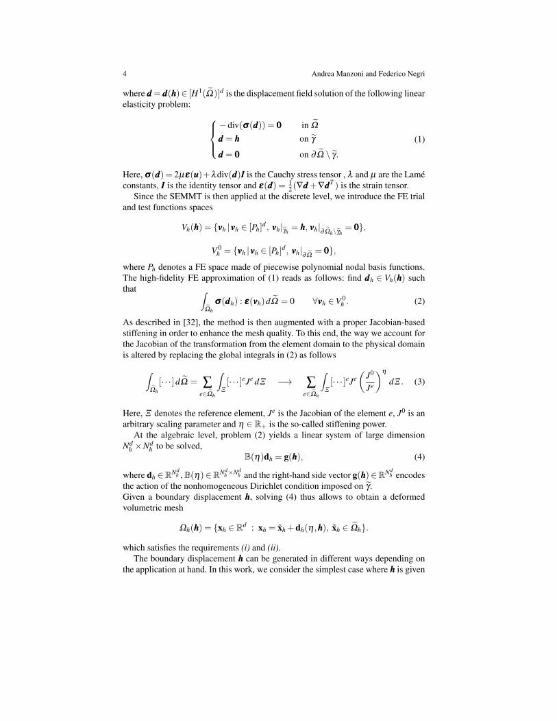
where ddd = ddd(hhh)∈ [H1(Ω)]d is the displacement field solution of the following linearelasticity problem:

−div(σσσ(ddd)) = 000 in Ω

ddd = hhh on γ

ddd = 000 on ∂Ω \ γ.

(1)

Here, σσσ(ddd) = 2µεεε(uuu)+λdiv(ddd)III is the Cauchy stress tensor , λ and µ are the Lameconstants, III is the identity tensor and εεε(ddd) = 1

2 (∇ddd +∇dddT ) is the strain tensor.Since the SEMMT is then applied at the discrete level, we introduce the FE trial

and test functions spaces

Vh(hhh) = vvvh |vvvh ∈ [Ph]d , vvvh|γh

= hhh, vvvh|∂Ωh\γh= 000,

V 0h = vvvh |vvvh ∈ [Ph]

d , vvvh|∂Ω= 000,

where Ph denotes a FE space made of piecewise polynomial nodal basis functions.The high-fidelity FE approximation of (1) reads as follows: find dddh ∈ Vh(hhh) suchthat ∫

Ωh

σσσ(dddh) : εεε(vvvh)dΩ = 0 ∀vvvh ∈V 0h . (2)

As described in [32], the method is then augmented with a proper Jacobian-basedstiffening in order to enhance the mesh quality. To this end, the way we account forthe Jacobian of the transformation from the element domain to the physical domainis altered by replacing the global integrals in (2) as follows

∫Ωh

[· · · ]dΩ = ∑e∈Ωh

∫Ξ

[· · · ]eJe dΞ −→ ∑e∈Ωh

∫Ξ

[· · · ]eJe(

J0

Je

)η

dΞ . (3)

Here, Ξ denotes the reference element, Je is the Jacobian of the element e, J0 is anarbitrary scaling parameter and η ∈ R+ is the so-called stiffening power.

At the algebraic level, problem (2) yields a linear system of large dimensionNd

h ×Ndh to be solved,

B(η)dh = g(hhh), (4)

where dh ∈RNdh , B(η)∈RNd

h×Ndh and the right-hand side vector g(hhh)∈RNd

h encodesthe action of the nonhomogeneous Dirichlet condition imposed on γ .Given a boundary displacement hhh, solving (4) thus allows to obtain a deformedvolumetric mesh

Ωh(hhh) = xh ∈ Rd : xh = xh +dh(η ,hhh), xh ∈ Ωh.

which satisfies the requirements (i) and (ii).The boundary displacement hhh can be generated in different ways depending on

the application at hand. In this work, we consider the simplest case where hhh is given


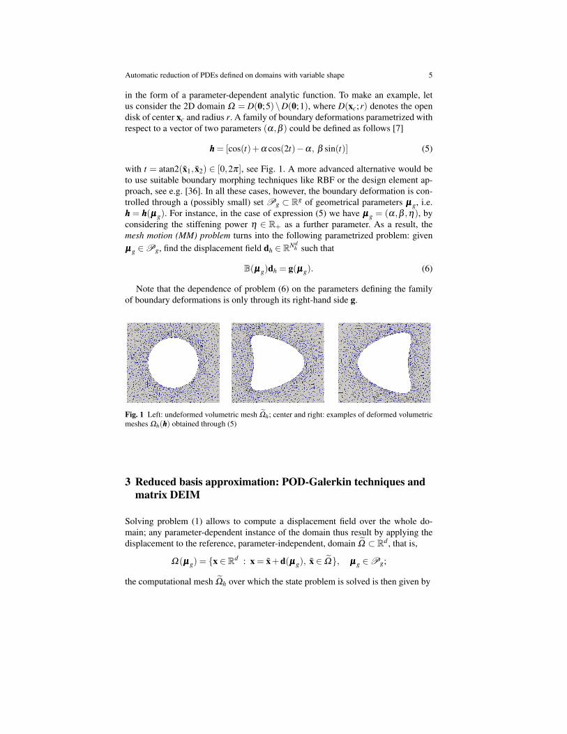
in the form of a parameter-dependent analytic function. To make an example, letus consider the 2D domain Ω = D(0;5)\D(0;1), where D(xc;r) denotes the opendisk of center xc and radius r. A family of boundary deformations parametrized withrespect to a vector of two parameters (α,β ) could be defined as follows [7]

hhh = [cos(t)+α cos(2t)−α, β sin(t)] (5)

with t = atan2(x1, x2) ∈ [0,2π], see Fig. 1. A more advanced alternative would beto use suitable boundary morphing techniques like RBF or the design element ap-proach, see e.g. [36]. In all these cases, however, the boundary deformation is con-trolled through a (possibly small) set Pg ⊂ Rg of geometrical parameters µµµg, i.e.hhh = hhh(µµµg). For instance, in the case of expression (5) we have µµµg = (α,β ,η), byconsidering the stiffening power η ∈ R+ as a further parameter. As a result, themesh motion (MM) problem turns into the following parametrized problem: givenµµµg ∈Pg, find the displacement field dh ∈ RNd

h such that

B(µµµg)dh = g(µµµg). (6)

Note that the dependence of problem (6) on the parameters defining the familyof boundary deformations is only through its right-hand side g.

Fig. 1 Left: undeformed volumetric mesh Ωh; center and right: examples of deformed volumetricmeshes Ωh(hhh) obtained through (5)

3 Reduced basis approximation: POD-Galerkin techniques andmatrix DEIM

Solving problem (1) allows to compute a displacement field over the whole do-main; any parameter-dependent instance of the domain thus result by applying thedisplacement to the reference, parameter-independent, domain Ω ⊂ Rd , that is,

Ω(µµµg) = x ∈ Rd : x = x+d(µµµg), x ∈ Ω, µµµg ∈Pg;

the computational mesh Ωh over which the state problem is solved is then given by


Ωh(µµµg) = xh ∈ Rd : xh = xh +dh(µµµg), xh ∈ Ωh, µµµg ∈Pg,

being dh = dh(µµµg) the solution of the high-fidelity problem (6). Since its solutionfor any parameter vector µµµg ∈Pg would be computationally expensive, we ratherapproximate the displacement field by relying on the RB method, whose main ingre-dients will be detailed in the following. Hence, we approximate dh(µµµg)≈VdN(µµµg)

as a linear combination of Nd (deformation) basis functions, being dN ∈ RNd a vec-tor of coefficients. The latter is the solution of a problem obtained by projecting thehigh-fidelity system (6) onto the basis V, as we shall describe later.

As a result, the set of parametrized domains we deal with is given byΩ

Nh (µµµg) = xN

h ∈ Rd : xNh = xh +VdN(µµµg), xh ∈ Ωh, µµµg ∈Pg

; (7)

provided that the error ‖dh(µµµg)−VdN(µµµg)‖ is sufficiently small – this is indeedensured by standard algorithms in the RB context – Ω N

h (µµµg) yields an accurateapproximation of Ωh(µµµg).

3.1 Formulation of the state problem

Let us now move to the state problem we finally want to solve. For the sake ofillustration, we consider as state problem the case of a scalar linear elliptic stationaryPDE, although the proposed technique can be extended to more general problemsin a straightforward way. Let us denote by W = W (µµµg) a suitable Hilbert space,defined over the parameter-dependent domain Ω(µµµg) ⊂ Rd ; in abstract form, theparametrized problem we focus on can be written as follows: given µµµ = (µµµg,µµµ p) ∈P = Pg×Pp ⊂ Rg+p, find u(µµµ) ∈W (µµµg) such that

a(u(µµµ),v;ddd(µµµg),µµµ p) = f (v;ddd(µµµg),µµµ p) ∀v ∈W (µµµg); (8)

here µµµ p denotes a vector of physical parameters only affecting the state problem.Note that the presence of the displacement ddd(µµµg), playing the role of known para-metrized field in (8), induces a dependence of both the bilinear form a(·, ·;ddd(µµµg),µµµ p) :W (µµµg)×W (µµµg)→C and the linear form f (·;ddd(µµµg),µµµ p) : W (µµµg)→C on µµµg, too.

Here we assume that a(·, ·;ddd(µµµg),µµµ p) is continuous and weakly coercive overW ×W , and that f (·;ddd(µµµg),µµµ p) is continuous, for any (µµµg,µµµ p), so that problem(8) admits a unique solution thanks to Necas theorem.

The high-fidelity, FE approximation of problem (8) can then be obtained upondefining a FE space Wh(µµµg) ⊂ W (µµµg) over the domain Ω N

h (µµµg), and seekinguh(µµµ) ∈Wh(µµµg) such that

a(uh(µµµ),vh;dN(µµµg),µµµ p) = f (vh;dN(µµµg),µµµ p) ∀vh ∈Wh(µµµg); (9)

note that we have already considered the RB approximation of the displacementfield. From an algebraic standpoint, problem (9) yields a linear system of large di-


mension Nuh ×Nu

h to be solved,

A(µµµ)uh(µµµ) = f(µµµ), (10)

where A(µµµ) = A(dN(µµµg); µµµ p) ∈ RNuh×Nu

h and f(µµµ) = f(dN(µµµg); µµµ p) ∈ RNuh .

3.2 POD-Galerkin reduced order models

Problems (6) and (10) share the same nature of parameter-dependent, high dimen-sional, linear systems arising from the discretization of two different second-orderparametrized PDEs. To solve them efficiently, we rely in both cases on the RBmethod, thus approximating the unknowns uh in a basis W ∈ RNu

h×Nu , dh in a ba-sis V ∈ RNd

h×Nd of reduced dimensions Nu Nuh , Nd Nd

h , i.e. uh(µµµ)≈WuN(µµµ),dh(µµµg) ≈ VdN(µµµg). Then, we enforce the orthogonality of the residual of eachequation to W and V, respectively, thus resulting in two Galerkin-RB problems un-der the following form: given µµµg ∈Pg, find dN(µµµg) ∈ RNd

BN(µµµg)dN(µµµg) = gN(µµµg), (11)

and then, given µµµ p ∈Pp, find uN(µµµ) ∈ RNu such that

AN(µµµ)uN(µµµ) = fN(µµµ), (12)

where the reduced matrices and vectors are given by

BN(µµµg) = VTB(µµµg)V, gN(µµµg) = VT g(µµµg), (13)

AN(µµµ) =WTA(dN(µµµg); µµµ p)W, fN(µµµ) =WT f(dN(µµµg); µµµ p). (14)

Here, we rely on the proper orthogonal decomposition (POD) method for theconstruction of the RB spaces. Once a set of snapshots of problems (6) and (10) hasbeen computed, the singular value decomposition of the corresponding correlationmatrices automatically yield optimal sets of orthonormal basis functions; see, e.g.,[25] for further details. Note that each snapshot of problem (10) is computed ona different spatial domain, depending on the value of µµµg; nevertheless, this is nota concern, since we have assumed that the mesh deformation induced by dh(µµµg)(and, correspondingly, by dN(µµµg)) does not affect the mesh connectivity and, as aresult, the connectivity graph of the matrix A(µµµ), too. The resulting POD-Galerkintechnique allows to obtain two problems (11) and (12) of very small dimension.

Assembling the reduced matrices and vectors as in (13)–(14) when µµµ ∈P variesis still too expensive in order to achieve efficient offline construction and online eval-uation of the RB problem. As already mentioned, if the system matrices (resp. vec-tors) can be expressed as an affine combination of constant matrices (resp. vectors)weighted by suitable parameter-dependent coefficients, each term of the weightedsums can be projected offline onto the RB space spanned by W, V, respectively. Forinstance, if we assume that the matrix A(µµµ) admits an affine decomposition


A(µµµ) =MA

∑q=1

θAq (µµµ)Aq, (15)

then

AN(µµµ) =WTA(µµµ)W=MA

∑q=1

θAq (µµµ)WTAqW,

where θ Aq : P 7→R and Aq ∈RNu

h×Nuh are given functions and matrices, respectively,

for q = 1, . . . ,MA; a similar affine decomposition made by M f terms is requiredfor the vector f(µµµ) as well. Since the reduced matrices WTAqW ∈ RNu×Nu can beprecomputed and stored offline, the online construction of the RB arrays in (14) fora given µµµ is fast and efficient as long as MA,M f Nu

h ; a similar conclusion clearlyholds for the RB arrays in (13), too.

In order to recover the affine structure (15) in those cases where the operatorA(µµµ) is nonaffine (i.e., (15) is not readily available), we must introduce a furtherlevel of reduction, called hyper-reduction; we thus refer to the resulting ROM ashyper-ROM (HROM). Here, we rely on DEIM to approximate the vectors f(µµµ) andg(µµµg), and its matrix variant MDEIM to approximate A(µµµ) and B(µµµg). A schematicsummary of the entire offline/online computational strategy is offered in Fig. 2.

µµµ1g, · · · ,µµµJ

g

collect solution andsystem snapshots:

dh(µµµjg)

B(µµµ jg), g(µµµ j

g)

MM-HROM SP-HROM

collect solution andsystem snapshots:

uh(µµµk)

A(µµµk), f(µµµk)

µµµ1, · · · ,µµµK

offline

MM-FOM

(M)DEIM

POD

SP-FOM

(M)DEIM

POD

µµµ = (µµµg,µµµ p) dN(µµµg) uN(µµµ)

online

Fig. 2 Scheme of offline and online phases for the geometry and state reduction. Here MM-FOMand MM-HROM refer to (6) and (11), respectively (i.e. the full and hyper-reduced order modelsfor the mesh motion (MM) problem). SP-FOM and SP-HROM refer instead to (10) and (12),respectively (i.e. the full and hyper-reduced order models for the state problem (SP))


3.3 Matrix DEIM

For the sake of space – and because of its relative novelty – here we only detail theway DEIM can be used to approximate a parameter-dependent matrix K(τ) : T 7→RNh×Nh , where τ denotes a generic parameters vector. Given K(τ) : T 7→ RNh×Nh ,the problem is to find M Nh functions θq : T 7→ R and parameter-independentmatrices Kq ∈ RNh×Nh , 1≤ q≤M, such that

K(τ)≈Km(τ) =M

∑q=1

θq(τ)Kq. (16)

The offline stage of this procedure consists of two main steps. First we expressK(τ) in vector format by stacking its columns, that is, we set k(τ) = vec(K(τ)) ∈RN2

h . Hence, (16) can be reformulated as: find ΦΦΦ ,θθθ(τ) such that

k(τ)≈ km(τ) = ΦΦΦθθθ(τ), (17)

where ΦΦΦ ∈ RN2h×M is a τ-independent basis and θθθ(τ) ∈ RM the corresponding

coefficients vector. Then, we apply DEIM as in [6] to a set of snapshots ΛΛΛ =[vec(K(τ1)), . . . ,vec(K(τns))] in order to obtain the basis ΦΦΦ and a set of interpo-lation indices I ⊂ 1, · · · ,N2

h. The former is computed by applying the POD tech-nique over the columns of ΛΛΛ , whereas the latter is iteratively selected by employingthe magic points algorithm [19].

During the online phase, given a new τ ∈T , we can compute Km(τ) as

Km(τ) = vec−1(ΦΦΦθθθ(τ)) with θθθ(τ) = ΦΦΦ−1I KI (τ), (18)

where ΦΦΦI and KI (τ) denote the matrices formed by the I rows of ΦΦΦ and K(τ),respectively. We point out that, for the sake of model order reduction, the crucial stepin the online evaluation of Km(τ) is the computation of KI (τ). Nevertheless, thisoperation can be performed efficiently when K(τ) results from a FE discretization ofa PDE operator, by employing the same assembly routine used for the high-fidelityproblem on the reduced mesh associated to the selected interpolation indices; see,e.g., [23] for further details.

4 Numerical example

As a proof of concept of the proposed technique, we consider a (direct) scatter-ing problem dealing with the Helmholtz equation. Scattering problems are meantto study the effect that a bounded obstacle (or scatterer) has on incident waves, de-pending on the geometrical properties of the body; these latter are considered asgeometrical parameters of interest. Such a problem is relevant in a wide range ofapplications such as the design of sonars and radars, medical imaging, geophysicalexploration, and nondestructive testing [7]. Given the incident wave, the goal of a


incoming wave

scattered wave


Du+k2u = 0 in W(µµµg)

u =eika·x on g(µµµg)

—u ·n iku = 0 on Gext .

(18)

Here k = w/c is the wave number, w = 2p f the angular frequency and c = 340cm s1 the speed of sound. The scattered wave is time-harmonic, but not necessaryplane, whereas the incident wave is considered to be a plane, time-harmonic waveui(x, t; µµµ) = ei(ka·xwt) with amplitude A = 1; here w denotes its frequency and a =(cos(a),sin(a))T its direction. We assume the scatterer to be a perfect conductor. Onthe boundary Gext we prescribe a first-order absorbing boundary condition, yieldingan approximation of the Sommerfeld radiation condition

limr!•

r

∂u∂ r

iku

= 0

usually imposed in the case of unbounded domains [35]. In addition to the geo-metrical parameters µµµg = (a,b ,h) encoding the shape of the obstacle B and thestiffening power, we also consider a vector of physical parameters µµµ p = (k,A,a) 2Pp Rp to model different scenarios where the wave number, as well as the direc-tion and amplitude of the incident wave can vary.

• MDEIM/DEIM on the mesh motion problem. A very small number of terms forapproximating the system is required.

• POD-Galerkin on this problem, comment figure 5. Very few basis functions areenough.

• Then, Helmholtz problem. The dependence on geometrical parameters yieldsnon negligible difficulties. The combined action of the wave number and geome-try, too. (Figure 6). As a result, spectra decay is slow for both system approxima-tion and state reduction. The reduced mesh (given by...) is mainly concentratedaround the obstacle, reasonable. Decay of the relative error, Figure 7

• Accenno al fatto che si possono anche considerare le stime dell’errore (criticitche vedo: cambia il dominio quando risolvi la deformazione con il ridotto, quindisi avrebbe bisogno di stimare l’errore sulla soluzione rispetto all’errore sullashape)

5 Conclusions

References

1. Baker, T.: Mesh movement and metamorphosis. Engrg. Comput. 18(3), 188–198 (2002)2. Ballarin, F., Manzoni, A., Rozza, G., Salsa, S.: Shape optimization by free-form deformation:

existence results and numerical solution for Stokes flows. J. Sci. Comput. 60(3), 537–563(2014)


Du+k2u = 0 in W(µµµg)

u =eika·x on g(µµµg)

—u ·n iku = 0 on Gext .

(18)

Here k = w/c is the wave number, w = 2p f the angular frequency and c = 340cm s1 the speed of sound. The scattered wave is time-harmonic, but not necessaryplane, whereas the incident wave is considered to be a plane, time-harmonic waveui(x, t; µµµ) = ei(ka·xwt) with amplitude A = 1; here w denotes its frequency and a =(cos(a),sin(a))T its direction. We assume the scatterer to be a perfect conductor. Onthe boundary Gext we prescribe a first-order absorbing boundary condition, yieldingan approximation of the Sommerfeld radiation condition

limr!•

r

∂u∂ r

iku

= 0

usually imposed in the case of unbounded domains [35]. In addition to the geo-metrical parameters µµµg = (a,b ,h) encoding the shape of the obstacle B and thestiffening power, we also consider a vector of physical parameters µµµ p = (k,A,a) 2Pp Rp to model different scenarios where the wave number, as well as the direc-tion and amplitude of the incident wave can vary.

• MDEIM/DEIM on the mesh motion problem. A very small number of terms forapproximating the system is required.

• POD-Galerkin on this problem, comment figure 5. Very few basis functions areenough.

• Then, Helmholtz problem. The dependence on geometrical parameters yieldsnon negligible difficulties. The combined action of the wave number and geome-try, too. (Figure 6). As a result, spectra decay is slow for both system approxima-tion and state reduction. The reduced mesh (given by...) is mainly concentratedaround the obstacle, reasonable. Decay of the relative error, Figure 7

• Accenno al fatto che si possono anche considerare le stime dell’errore (criticitche vedo: cambia il dominio quando risolvi la deformazione con il ridotto, quindisi avrebbe bisogno di stimare l’errore sulla soluzione rispetto all’errore sullashape)

5 Conclusions

References




4 Numerical example

As a proof of concept of the proposed technique, we consider a (direct) scatter-ing problem dealing with the Helmholtz equation. Scattering problems are meantto study the effect that a bounded obstacle (or scatterer) has on incident waves, de-pending on the geometrical properties of the body; these latter are considered asgeometrical parameters of interest. Such a problem is relevant in a wide range ofapplications such as the design of sonars and radars, medical imaging, geophysicalexploration, nondestructive testing [7]. Given the incident wave, the goal of a directscattering problem is to determine the scattered wave for the known obstacle; froma numerical standpoint, this is also a premise in view of the (indeed, very challeng-ing) inverse scattering problem, in which the obstacle shape has to be reconstructedfrom far-field measurements. Helmholtz equations have already been tackled by RBmethods, see, e.g. [29, 30, 18].

Let B Rd , d = 2,3, the domain of an object with boundary g = ∂B, and assumethat g = g(µµµg) is parametrized with respect to a vector of geometrical parametersµµµg 2Pg Rg. The exterior domain is defined by the unbounded region R =Rd \B;here we restrict ourselves to the case d = 2, although everything can be simplyextended to the case d = 3 as well. Instead of considering an exterior acousticsproblem in an unbounded domain, we truncate this latter by an artificial boundaryGext where local absorbing boundary conditions are imposed; as a result, we dealwith a bounded computational domain W , see Fig. 3.

Bincoming wave

scattered wave

Fig. 3 Sketch of the domain and of the underlying physics; background coloring given by ¬(u)for µµµg = (0.4,1.2,1.2), k = 5, a = p/6.

Here we consider the propagation of time harmonic waves, for which the acousticpressure P can be separated as P(x, t; µµµ) = ¬(u(x; µµµ)eiwt); the complex amplitudeu = u(x; µµµ) then satisfies the Helmholtz equation


4 Numerical example

As a proof of concept of the proposed technique, we consider a (direct) scatter-ing problem dealing with the Helmholtz equation. Scattering problems are meantto study the effect that a bounded obstacle (or scatterer) has on incident waves, de-pending on the geometrical properties of the body; these latter are considered asgeometrical parameters of interest. Such a problem is relevant in a wide range ofapplications such as the design of sonars and radars, medical imaging, geophysicalexploration, nondestructive testing [7]. Given the incident wave, the goal of a directscattering problem is to determine the scattered wave for the known obstacle; froma numerical standpoint, this is also a premise in view of the (indeed, very challeng-ing) inverse scattering problem, in which the obstacle shape has to be reconstructedfrom far-field measurements. Helmholtz equations have already been tackled by RBmethods, see, e.g. [29, 30, 18].

Let B Rd , d = 2,3, the domain of an object with boundary g = ∂B, and assumethat g = g(µµµg) is parametrized with respect to a vector of geometrical parametersµµµg 2Pg Rg. The exterior domain is defined by the unbounded region R =Rd \B;here we restrict ourselves to the case d = 2, although everything can be simplyextended to the case d = 3 as well. Instead of considering an exterior acousticsproblem in an unbounded domain, we truncate this latter by an artificial boundaryGext where local absorbing boundary conditions are imposed; as a result, we dealwith a bounded computational domain W , see Fig. 3.

Bincoming wave

scattered wave

Fig. 3 Sketch of the domain and of the underlying physics; background coloring given by ¬(u)for µµµg = (0.4,1.2,1.2), k = 5, a = p/6.

Here we consider the propagation of time harmonic waves, for which the acousticpressure P can be separated as P(x, t; µµµ) = ¬(u(x; µµµ)eiwt); the complex amplitudeu = u(x; µµµ) then satisfies the Helmholtz equation

Fig. 3 Sketch of the domain and of the underlying physics; background coloring given by ℜ(u)for µµµg = (−0.4,1.2,1.2), κ = 5, a = π/6.

direct scattering problem is to determine the scattered wave for the known obsta-cle; from a numerical standpoint, this is also a premise in view of the (indeed, verychallenging) inverse scattering problem, in which the obstacle shape has to be re-constructed from far-field measurements. Helmholtz equations have already beentackled by RB methods, see, e.g. [28, 29, 17].

Let B⊂Rd , d = 2,3, the domain of an object with boundary γ = ∂B, and assumethat γ = γ(µµµg) is parametrized with respect to a vector of geometrical parametersµµµg ∈Pg⊂Rg. The exterior domain is defined by the unbounded region R =Rd \B;here we restrict ourselves to the case d = 2, although everything can be simplyextended to the case d = 3 as well. Instead of considering an exterior acousticsproblem in an unbounded domain, we truncate this latter by an artificial boundaryΓext where local absorbing boundary conditions are imposed; as a result, we dealwith a bounded computational domain Ω , see Fig. 3.

Here we consider the propagation of time harmonic waves, for which the acousticpressure P can be separated as P(x, t; µµµ) = ℜ(u(x; µµµ)e−iωt); the complex amplitudeu = u(x; µµµ) then satisfies the Helmholtz equation

∆u+κ2u = 0 in Ω(µµµg)

u =−eiκ a·x on γ(µµµg)

∇u ·n− iκu = 0 on Γext .

(19)

Here κ = ω/c is the wave number, ω = 2π f the angular frequency and c = 340cm s−1 the speed of sound. The scattered wave is time-harmonic, but not necessaryplane, whereas the incident wave is considered to be a plane, time-harmonic waveui(x, t; µµµ)= ei(κa·x−ωt) with amplitude A= 1 and direction a=(cos(a),sin(a))T . Onthe boundary Γext we prescribe a first-order absorbing boundary condition, yieldingan approximation of the Sommerfeld radiation condition


limr→∞

r(

∂u∂ r− iku

)= 0

usually imposed in the case of unbounded domains [34]. In addition to the geomet-rical parameters µµµg = (α,β ,η) encoding the shape of the obstacle B and the stiffen-ing power, we also consider a vector of physical parameters µµµ p = (κ,a)∈Pp ⊂Rp

to model different scenarios where the wave number, as well as the direction, of theincident wave can vary.

We now apply the methodology developed in the previous sections to problem(19). The full-order model for the state Helmholtz problem is given by a Pbubble

1 finiteelement approximation of (19), yielding a linear system of dimension Nu

h = 147272obtained using a mesh made of 97934 triangular elements. Similarly, the full-ordermodel for the mesh motion problem (1) is built using Pbubble

1 finite elements, yieldinga linear system of dimension Nd

h = 294544. Concerning the parameter range, weselect α ∈ [−1/2,1/2], β ∈ [−0.81.2], η ∈ [0,1.4]; instead, physical parametersrange in κ ∈ [2,5], a ∈ [0,π/6].

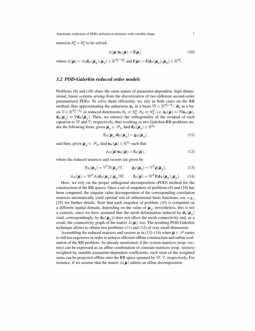
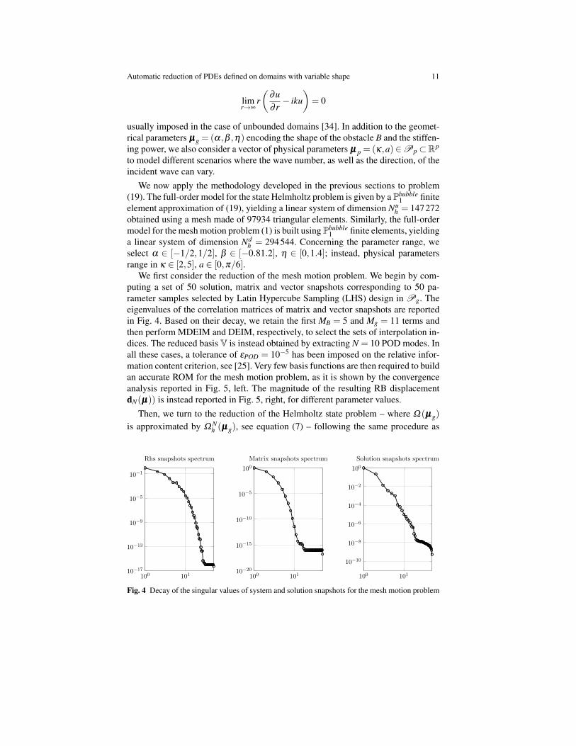
We first consider the reduction of the mesh motion problem. We begin by com-puting a set of 50 solution, matrix and vector snapshots corresponding to 50 pa-rameter samples selected by Latin Hypercube Sampling (LHS) design in Pg. Theeigenvalues of the correlation matrices of matrix and vector snapshots are reportedin Fig. 4. Based on their decay, we retain the first MB = 5 and Mg = 11 terms andthen perform MDEIM and DEIM, respectively, to select the sets of interpolation in-dices. The reduced basis V is instead obtained by extracting N = 10 POD modes. Inall these cases, a tolerance of εPOD = 10−5 has been imposed on the relative infor-mation content criterion, see [25]. Very few basis functions are then required to buildan accurate ROM for the mesh motion problem, as it is shown by the convergenceanalysis reported in Fig. 5, left. The magnitude of the resulting RB displacementdN(µµµ)) is instead reported in Fig. 5, right, for different parameter values.

Then, we turn to the reduction of the Helmholtz state problem – where Ω(µµµg)

is approximated by Ω Nh (µµµg), see equation (7) – following the same procedure as

100 10110−17

10−13

10−9

10−5

10−1

Rhs snapshots spectrum

100 10110−20

10−15

10−10

10−5

100Matrix snapshots spectrum

100 101

10−10

10−8

10−6

10−4

10−2

100Solution snapshots spectrum

Fig. 4 Decay of the singular values of system and solution snapshots for the mesh motion problem


0 2 4 6 8 1010−5

10−4

10−3

10−2

10−1

100

N

‖dh − dN‖/‖dh‖

Fig. 5 Left: Relative error on the solution of the mesh motion problem (averaged over a test sampleof 100 parameter values). Right: magnitude of the displacement dN(µµµ) for different parametervalues

above. Regarding the system approximation, in this case MA = 60 and M f = 142terms are selected out of 400 matrix and vector snapshots; concerning state reduc-tion, we retain N = 120 basis functions, see Fig. 6.

Note that the decay of the eigenvalues of the correlation matrix is much slowerthan in the previous case highlighting a stronger variability of uh(µµµ) – as well asof the problem arrays A(µµµ), f(µµµ) – with respect to combined variations of bothgeometrical and physical parameters. This also translates into a much slower errorconvergence with respect to the RB dimension Nu, see Fig. 7, right. The resultingreduced mesh (see Fig. 7, left) is made of 291 elements, corresponding to about the0.3% of the original ones; note that they concentrate around the obstacle, i.e. in theregion where problem sensitivity to shape variations is higher. Some instances ofthe solution uN(µµµ) to the Helmholtz equation obtained with the proposed techniqueare finally shown in Fig. 8; as a concluding remark, we point out that the online

100 101 102

10−10

10−8

10−6

10−4

10−2

100Rhs snapshots spectrum

100 101 10210−17

10−13

10−9

10−5

10−1

Matrix snapshots spectrum

100 101 102

10−7

10−5

10−3

10−1

Solution snapshots spectrum

Fig. 6 Decay of the singular values of system and solution snapshots for the Helmholtz problem


0 20 40 60 80 100 12010−3

10−2

10−1

100

N

‖uh − uN‖/‖uh‖

Fig. 7 Left: zoom of the reduced mesh (red elements) around the object. Right: relative error onthe solution of the Helmholtz problem (averaged over a testing set of 200 parameter values)

Fig. 8 ℜ(uN(µµµ)) for different values of the parameters

solution of both the reduced mesh motion (11) and the reduced Helmholtz problem(12) problems takes about 0.26s, thus realizing a computational speedup of about25 times with respect to the finite element FOM.

5 Conclusions

In this work we have presented a general and automatic way to deal with the effi-cient solution of parameterized PDEs defined on domains with variable shape. Thisframework combines a mesh motion technique relying on the solution of a solidextension problem, a POD-Galerkin reduced basis method, and a further hyper-reduction stage based on DEIM/MDEIM techniques. Compared to already exist-ing strategies for handling mesh deformations in the RB context, the technique ex-ploited in this work allows to directly define global domain deformations startingfrom boundary parametrizations. Indeed, relying on boundary – rather than volume– parametrizations is the most common and intuitive way to handle shape variationswhen design optimization is performed.

Although the proposed framework has been tested on a simplified case, where asingle explicit boundary parametrization has been considered, its capabilities lookpromising in view of tackling a wider range of problems. For instance, it allowsto handle different types of parametrizations simultaneously, each one defined ona separate portion of the boundary. Furthermore, it also applies in the case where a


database of boundary deformations results from the solution of a different problem –rather than from an explicit formula. This is the case, e.g., of fluid-structure interac-tion problems, where the deformation of the fluid-structure interface is an unknownof the problem itself; further work is ongoing in this respect.

References



3. Barrault, M., Maday, Y., Nguyen, N.C., Patera, A.T.: An ‘empirical interpolation’ method:application to efficient reduced-basis discretization of partial differential equations. C. R.Math. Acad. Sci. Paris 339(9), 667–672 (2004)

4. Canuto, C., Tonn, T., Urban, K.: A posteriori error analysis of the reduced basis method fornon-affine parameterized nonlinear PDEs. SIAM J. Numer. Anal. 47(3), 2001–2022 (2009)

5. Carlberg, K., Tuminaro, R., Boggs, P.: Preserving Lagrangian structure in nonlinear modelreduction with application to structural dynamics. SIAM J. Sci. Comput. 37(2), B153–B184(2015)

6. Chaturantabut, S., Sorensen, D.C.: Nonlinear model reduction via discrete empirical interpo-lation. SIAM J. Sci. Comput. 32(5), 2737–2764 (2010)

7. Colton, D., Kress, R.: Inverse Acoustic and Electromagnetic Scattering Theory. Springer-Verlag, Berlin (2012)

8. Deparis, S., Forti, D., Quarteroni, A.: A rescaled localized radial basis function interpola-tion on non-cartesian and nonconforming grids. SIAM J. Sci. Comput. 36(6), A2745–A2762(2014)

9. Deparis, S., Løvgren, A.E.: Stabilized reduced basis approximation of incompressible three-dimensional Navier-Stokes equations in parametrized deformed domains. J. Sci. Comput.50(1), 198–212 (2012)

10. Forti, D., Rozza, G.: Efficient geometrical parametrisation techniques of interfaces forreduced-order modelling: application to fluid-structure interaction coupling problems. Int.J. Comput. Fluid. Dyn. 28(3–4), 158–169 (2014)

11. Gordon, W., Hall, C.: Construction of curvilinear co-ordinate systems and applications to meshgeneration. Int. J. Numer. Methods Engrg. 7(4), 461–477 (1973)

12. Grepl, M.A., Maday, Y., Nguyen, N.C., Patera, A.T.: Efficient reduced-basis treatment of non-affine and nonlinear partial differential equations. ESAIM Math. Modelling Numer. Anal.41(3), 575–605 (2007)

13. Helenbrook, B.: Mesh deformation using the biharmonic operator. Int. J. Numer. MethodsEngrg. 56(7), 1007–1021 (2003)

14. Hesthaven, J., Rozza, G., Stamm, B.: Certified Reduced Basis Methods for Parametrized Par-tial Differential Equations. SpringerBriefs in Mathematics. Springer (2016)

15. Iapichino, L., Quarteroni, A., Rozza, G.: A reduced basis hybrid method for the coupling ofparametrized domains represented by fluidic networks. Comput. Methods Appl. Mech. Engrg.221–222, 63–82 (2012)

16. Jaggli, C., Iapichino, L., Rozza, G.: An improvement on geometrical parameterizations bytransfinite maps. C. R. Acad. Sci. Paris. Ser. I 352(3), 263–268 (2014)

17. Lassila, T., Manzoni, A., Rozza, G.: On the approximation of stability factors for generalparametrized partial differential equations with a two-level affine decomposition. ESAIMMath. Modelling Numer. Anal. 46(6), 1555–1576 (2012)

18. Lassila, T., Rozza, G.: Parametric free-form shape design with PDE models and reduced basismethod. Comput. Methods Appl. Mech. Engrg. 199(23–24), 1583–1592 (2010)


19. Maday, Y., Nguyen, N.C., Patera, A.T., Pau, G.S.H.: A general multipurpose interpolationprocedure: the magic points. Commun. Pure Appl. Anal. 8(1), 383–404 (2009)

20. Manzoni, A., Quarteroni, A., Rozza, G.: Model reduction techniques for fast blood flow simu-lation in parametrized geometries. Int. J. Numer. Methods Biomed. Engng. 28(6–7), 604–625(2012)

21. Manzoni, A., Quarteroni, A., Rozza, G.: Shape optimization of cardiovascular geometries byreduced basis methods and free-form deformation techniques. Int. J. Numer. Methods Fluids70(5), 646–670 (2012)

22. Manzoni, A., Salmoiraghi, F., Heltai, L.: Reduced basis isogeometric methods (RB-IGA) forthe real-time simulation of potential flows about parametrized NACA airfoils. Comput. Meth.Appl. Mech. Engrg. 284, 1147 – 1180 (2015)

23. Negri, F., Manzoni, A., Amsallem, D.: Efficient model reduction of parametrized systems bymatrix discrete empirical interpolation. J. Comp. Phys. 303, 431–454 (2015)

24. Nguyen, N.C.: A posteriori error estimation and basis adaptivity for reduced-basis approxi-mation of nonaffine-parametrized linear elliptic partial differential equations. J. Comp. Phys.227, 983–1006 (2007)

25. Quarteroni, A., Manzoni, A., Negri, F.: Reduced Basis Methods for Partial Differential Equa-tions. An Introduction, Unitext, vol. 92. Springer (2016)

26. Rozza, G., Huynh, D.B.P., Patera, A.T.: Reduced basis approximation and a posteriori er-ror estimation for affinely parametrized elliptic coercive partial differential equations. Arch.Comput. Methods Engrg. 15, 229–275 (2008)

27. Rozza, G., Lassila, T., Manzoni, A.: Reduced basis approximation for shape optimization inthermal flows with a parametrized polynomial geometric map. In: J.S. Hesthaven, E. Rønquist(eds.) Spectral and High Order Methods for Partial Differential Equations. Selected papersfrom the ICOSAHOM ’09 conference, June 22-26, Trondheim, Norway, Lecture Notes inComputational Science and Engineering, vol. 76, pp. 307–315. Springer, Berlin Heidelberg(2011)

28. Sen, S.: Reduced basis approximation and a posteriori error estimation for non-coercive el-liptic problems: application to acoustics. Ph.D. thesis, Massachusetts Institute of Technology(2007)

29. Sen, S., Veroy, K., Huynh, D.B.P., Deparis, S., Nguyen, N.C., Patera, A.T.: “Natural norm” aposteriori error estimators for reduced basis approximations. J. Comp. Phys. 217(1), 37–62(2006)

30. Staten, M., Owen, S., Shontz, S., Salinger, A., Coffey, T.: A comparison of mesh morph-ing methods for 3D shape optimization. In: Proceedings of the 20th international meshingroundtable, pp. 293–311. Springer (2011)

31. Stein, K., Tezduyar, T., Benney, R.: Mesh moving techniques for fluid-structure interactionswith large displacements. J. Appl. Mech. 70(1), 58–63 (2003)

32. Stein, K., Tezduyar, T., Benney, R.: Automatic mesh update with the solid-extension meshmoving technique. Comput. Meth. Appl. Mech. Engrg. 193(21), 2019–2032 (2004)

33. Tezduyar, T., Behr, M., Mittal, S., Johnson, A.: Computation of unsteady incompressible flowswith the stabilized finite element methods: Space-time formulations, iterative strategies andmassively parallel implementations. In: New methods in transient analysis, vol. 246/AMD,pp. 7–24. ASME, New York (1992)

34. Thompson, L.: A review of finite-element methods for time-harmonic acoustics. J. Acoust.Soc. Am. 119(3), 1315–1330 (2006)

35. Wirtz, D., Sorensen, D.C., Haasdonk, B.: A Posteriori Error Estimation for DEIM ReducedNonlinear Dynamical Systems. SIAM J. Sci. Comput. 36(2), A311–A338 (2014)

36. Zahr, M.J., Farhat, C.: Progressive construction of a parametric reduced-order model for PDE-constrained optimization. Int. J. Numer. Methods Engng. 102(5), 1111–1135 (2015)

Recent publications:

MATHEMATICS INSTITUTE OF COMPUTATIONAL SCIENCE AND ENGINEERING Section of Mathematics

Ecole Polytechnique Fédérale (EPFL)

CH-1015 Lausanne

07.2016 M. LANGE, S. PALAMARA, T. LASSILA, C. VERGARA, A. QUARTERONI, A.F. FRANGI: Improved hybrid/GPU algorithm for solving cardiac electrophysiology problems on

Purkinje networks 08.2016 ALFIO QUARTERONI, ALESSANDRO VENEZIANI, CHRISTIAN VERGARA: Geometric multiscale modeling of the cardiovascular system, between theory and

practice 09.2016 ROCCO M. LANCELLOTTI, CHRISTIAN VERGARA, LORENZO VALDETTARO,

SANJEEB BOSE, ALFIO QUARTERONI: Large Eddy simulations for blood fluid-dynamics in real stenotic carotids 10.2016 PAOLO PACCIARINI, PAOLA GERVASIO, ALFIO QUARTERONI: Spectral based discontinuous Galerkin reduced basis element method for parametrized

Stokes problems 11.2016 ANDREA BARTEZZAGHI, LUCA DEDÈ, ALFIO QUARTERONI: Isogeometric analysis of geometric partial differential equations 12.2016 ERNA BEGOVIĆ KOVAČ, DANIEL KRESSNER: Structure-preserving low multilinear rank approximation of antisymmetric tensors 13.2016 DIANE GUIGNARD, FABIO NOBILE, MARCO PICASSO: A posteriori error estimation for the steady Navier-Stokes equations in random

domains 14.2016 MATTHIAS BOLTEN, KARSTEN KAHL, DANIEL KRESSNER, FRANCISCO MACEDO, SONJA

SOKOLOVIĆ: Multigrid methods combined with low-rank approximation for tensor structured

Markov chains 15.2016 NICOLA GUGLIELMI, MUTTI-UR REHMAN, DANIEL KRESSNER: A novel iterative method to approximate structured singular values 16.2016 YVON MADAY, ANDREA MANZONI, ALFIO QUARTERONI : An online intrinsic stabilitzation strategy for the reduced basis approximation of

parametrized advection-dominated 17.2016 ANDREA MANZONI, LUCA PONTI : An adjoint-based method for the numerical approximation of shape optimization

problems in presence of fluid-structure interaction 18.2016 STEFANO PAGANI, ANDREA MANZONI, ALFIO QUARTERONI: A reduced basis ensemble Kalman filter for state/parameter identification in large-

scale nonlinear dynamical systems 19.2016 ANDREA MANZONI, FEDERICO NEGRI : Automatic reduction of PDEs defined on domains with variable shape

automatic reduction of pdes defined on domains with...

Documents