354 JOURNAL OF THE INSTITUTE OF BREWING

Automatic Detection of Critical Points in Bottling Plants with a Model-based

Diagnosis Algorithm

Stefan Flad*, Peter Struss and Tobias Voigt

ABSTRACT

J. Inst. Brew. 116(4), 354–359, 2010

The efficiency of bottling plants typically ranges between 40 to 70%. Automatic conditioning monitoring helps to find critical points in a plant and supports the operator in optimizing the plant. But bottling plants are complex lines of several linked machines and currently critical points can only be identified manually. This paper presents a model-based efficiency analysis tool. It automatically localizes critical points that decrease the efficiency of the whole plant and the tool is adaptable to differ-ent plants solely through parameterization. The algorithm com-pares the behaviour of a plant with an OK-model of the plant. If there are inconsistencies, the commercial tool RAZ´R finds a failure model that is consistent with the observed plant behav-iour, thus localizing the component that causes downtime of the filler. The algorithm succeeds in identifying the cause of the downtime in 90% of the cases. A demonstrator application, which runs on different plants, has been implemented and re-quires only simple adaptation steps. The algorithm only needs information about the configuration of the plant and the produc-tion data, which normally exists in automated plants. In the fu-ture, it is expected that the project partners will integrate the algorithm with their PDA-systems, such that the model-based analysis will help to increase the efficiency of bottling plants.

Key words: bottling plants, efficiency analysis, model-based diagnosis.

INTRODUCTION Bottling plants are complex production lines with sev-

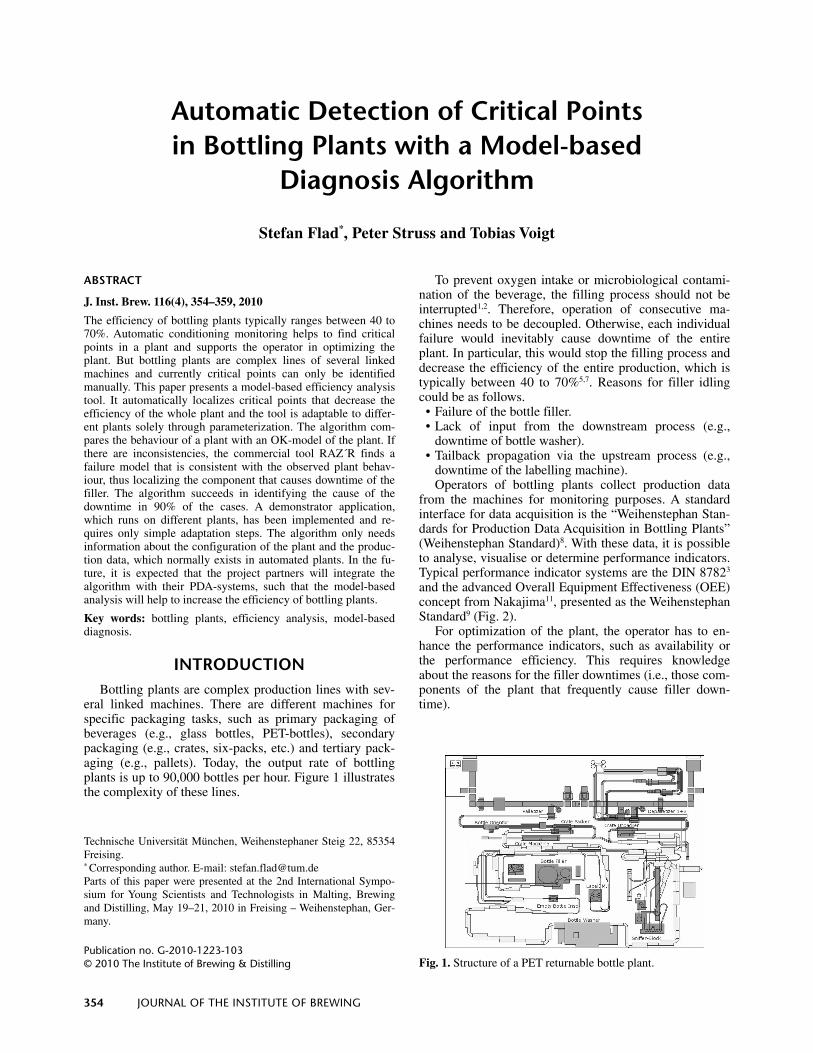
eral linked machines. There are different machines for specific packaging tasks, such as primary packaging of beverages (e.g., glass bottles, PET-bottles), secondary packaging (e.g., crates, six-packs, etc.) and tertiary pack-aging (e.g., pallets). Today, the output rate of bottling plants is up to 90,000 bottles per hour. Figure 1 illustrates the complexity of these lines.

To prevent oxygen intake or microbiological contami-nation of the beverage, the filling process should not be interrupted1,2. Therefore, operation of consecutive ma-chines needs to be decoupled. Otherwise, each individual failure would inevitably cause downtime of the entire plant. In particular, this would stop the filling process and decrease the efficiency of the entire production, which is typically between 40 to 70%5,7. Reasons for filler idling could be as follows.

• Failure of the bottle filler. • Lack of input from the downstream process (e.g.,

downtime of bottle washer). • Tailback propagation via the upstream process (e.g.,

downtime of the labelling machine). Operators of bottling plants collect production data

from the machines for monitoring purposes. A standard interface for data acquisition is the “Weihenstephan Stan-dards for Production Data Acquisition in Bottling Plants” (Weihenstephan Standard)8. With these data, it is possible to analyse, visualise or determine performance indicators. Typical performance indicator systems are the DIN 87823 and the advanced Overall Equipment Effectiveness (OEE) concept from Nakajima11, presented as the Weihenstephan Standard9 (Fig. 2).

For optimization of the plant, the operator has to en-hance the performance indicators, such as availability or the performance efficiency. This requires knowledge about the reasons for the filler downtimes (i.e., those com-ponents of the plant that frequently cause filler down-time).

Technische Universität München, Weihenstephaner Steig 22, 85354Freising. * Corresponding author. E-mail: stefan.flad@tum.de Parts of this paper were presented at the 2nd International Sympo-sium for Young Scientists and Technologists in Malting, Brewingand Distilling, May 19–21, 2010 in Freising – Weihenstephan, Ger-many.

Publication no. G-2010-1223-103 © 2010 The Institute of Brewing & Distilling

Fig. 1. Structure of a PET returnable bottle plant.

VOL. 116, NO. 4, 2010 355

Currently, this is subject to a manual analysis. In order to avoid relying on statistically insignificant results from individual snap shots, operators of plants need automatic tools to support this analysis.

Goals

A research project – called LineMod – was started to find automatic solutions for plant optimisation. The pro-ject was funded under FVNr. 233 ZGB by the Federal Ministry of Economics and Technology (BMWi) through the working group of the industrial research association “Otto von Guericke” e. V.

The main goal of the project was to develop algorithms and a system for automating the identification of filler downtime causes. Based on the results, a plant operator should be able to optimize the plant efficiency and en-hance availability and performance efficiency. A second goal was to develop a flexible diagnosis algorithm. It had to be adaptable to different plants only with fitting pa-rameters and describing the structure of the plant. There-fore, it was decided to use a model-based diagnosis algo-rithm.

METHODS Model-based diagnosis

A library of component models was generated that al-lows one to configure models of different plants. For typi-cal bottling plants, four basic component models are needed. These are as follows.

• Material Transport (MT) for conveyors and machines. • Separate Element (SE) for crate unpacker and depallet-

izer. • Combine Element (CE) for crate packer and palletizer. • Transportation Connector (TC), a virtual component to

connect the elements. In the following sections, the modelling assumptions

and the main concept of the components, using MT as an example, are described. The other components were built in a similar way and are described in the report by Struss et al.12

Modelling assumptions

The most important assumptions underlying the mate-rial transportation models presented here, which are ful-filled in our project domain (under normal conditions), but should also apply to a much broader class of prob-lems, are listed as follows.

• The transported objects are rigid bodies with fixed spa-tial extensions and are not significantly deformed through transportation.

• They are transported with a fixed orientation (such as crates), or the orientation does not affect transportation times significantly (e.g., due to a symmetric cross-sec-tion, as for bottles).

• There is no interaction among the objects or between objects and the components that have a significant im-pact on the transportation process (such as bouncing).

• Objects can move only in the direction of the motion of the transportation means (or not at all).

A model of a material transportation element with buffer

In order to present the essentials of the modelling ap-proach, some sort of archetype of model, which can be specialized or extended to accommodate other kinds of machines, was considered. This is a machine that includes the following.

• Has one input and one output with vin, vout being the re-spective speeds of the means for transportation (e.g., belts).

• Possibly transforms or modifies one kind of object (as, for instance, cleaning of bottles), but does not amalga-mate several objects to form a new one.

• Has a buffer with a (constant) capacity C. The process of buffering the objects can be fairly ran-

dom, where bottles may gather in bulks. However, it is assumed, that (under normal behaviour) no object is pre-vented from approaching the output unless it is blocked by other objects ahead, waiting for output. For instance, within the bottle conveyor, its shape and several parallel belts with different speeds ensure that bottles are not left

Fig. 2. Advanced OEE-concept9.

356 JOURNAL OF THE INSTITUTE OF BREWING

in a corner, but are pushed towards the “ideal” fastest belt, if there is space. The intuition behind the model can be best described in terms of three fundamental concepts and four “behaviour rules”, each of which is first introduced informally and then turned into equations. One of the problems to be solved stems from the fact that a local ma-chine model in isolation cannot determine whether an actual flow occurs at its input and output. But it can and has to express the limits on the machine’s potential to take in or output objects. Table I shows the material transporter and Fig. 3 illustrates it.

Concept 1. The potential input and output flow, in.qpot and out.qpot, represent the maximal flow the machine can accept or generate, dependent on its internal state.

The actual flows are represented by two different vari-ables, in.qact and out.qact. The first restriction is determined by rule 1.

Rule 1. The potential input flow is given by the input speed of the transportation element, unless the buffer is full. In this case, it cannot be higher than the actual output flow.

In the mathematical model (Table I), this rule is for-malized by equation 1, where d0 denotes the diameter of the object cross-section and B is the filling degree of the buffer (in terms of number of objects). It involves the as-sumption that an actual outflow generates the potential for intake instantaneously, which is not true in practice and, hence, a reason for expressing tolerance intervals with

values and time. Note that all speeds and flows were taken as positive, as their sign is determined by their association with the intrinsic direction of the transportation element. Computing B is straightforward with rule 2.

Rule 2. The change in the total number of buffered ob-jects is determined by the actual input and output flows.

The respective equation 2 indicates that B will be com-puted by integrating the difference of the actual flows. Setting up the model fragments for the potential output flow is based on the second key idea concept 2.

Concept 2. Bout denotes the number of buffered output objects at time t (i.e., the number of objects that can possi-bly be subject to output at this time). Before this crucial concept is clarified, its intuitive understanding is used and the third concept for formulating the rule for the potential output flow is concept 3.

Concept 3. The minimal transportation time td, is the time an object needs to get directly from the input to the output (i.e., if it is not delayed by other objects that are piling up).

Rule 3. The potential output flow is determined solely by the output speed, if there is more than one buffered output object. Otherwise, it cannot be higher than the ac-tual input flow at the time reduced by the minimal trans-portation time.

One should be aware that in the second case, each sin-gle object may (potentially) leave the output with the speed vout. However, if the input flow at the time when it entered was lower, there will be a gap occurring after the output of the object, which makes the (average) flow lower than vout.

As a special case, the potential output flow becomes zero, if B0 is zero, which implies that the actual input flow was zero at the respective shifted time.

Again, the respective equation 3 in Table I formalizes this. Computing Bout also involves the minimal transporta-tion time td. If an object entered the transportation element later than time t - td, it cannot possibly reach the output at time t and, hence, cannot become part of the buffered out-put objects. If it entered earlier, it may or may not have already left the output before t, depending on how the actual output flow reduced Bout. This consideration is cap-tured by rule 4.

Rule 4. The change in the number of buffered output objects at time t is determined by the actual input flow at time t - td diminished by the actual outflow at time t.

Hence, Bout is also obtained by integration according to equation 4, which completes the model of the transporta-tion element with buffer. Note, that Bout is not necessarily the number of objects that form a contiguous pile in front of the output. It could be less, because the last objects that joined the pile entered later than t - td.

Other model elements

Another class of machines produces an output by com-bining objects of different kinds, as for instance the pack-aging of 20 bottles in a crate. The ratio of the number of different objects participating in this combination is usu-ally not arbitrary, but is specified exactly. This ratio links the various potential and actual inflows and the outflow, which is then limited by the “slowest” input flow (relative to the ratio of the respective object type).

Table I. Model of material transporter.

State variables

B objects in buffer Bout objects buffered for immediate output vin velocity of input transportation means vout velocity of output transportation means td minimal transportation time

Parameters

d0 diameter of transported object (in transportation plane) C capacity

Interface variables

in.qpot potential inflow [objects/s] out.qpot potential outflow [objects/s] in.qact actual inflow [objects/s] out.qact actual outflow [objects/s]

Equations

in.qpot(t) = vin(t) / d0 if B(t) < C (1) in.qpot(t) = min (vin(t) / d0, out.qact(t)) if B(t) = C

(2) dB/dt = in.qact(t) – out.qact(t) out.qpot(t)= vout(t) / d0 if Bout(t) ≥ 1 (3) out.qpot(t)= min (in.qact(t – td), vout(t) / d0) else

(4) dBout(t) /dt = in.qact(t – td) – out.qact(t)

Fig. 3. Schematic model of a material transporter.

VOL. 116, NO. 4, 2010 357

The counterpart to this very generic combination ele-ment is the separation element, with unpackers being a subclass, in which the slowest actual outflow of a decom-position result limits the potential inflow of the composite object.

For connection of the various elements, the virtual component transportation connector was modelled. The transportation connector links the potential and actual flows of two elements.

Rule TC. The actual output flow of a machine is lim-ited by both its own potential output flow and the poten-tial input flow of the following machine (and equal to the actual input flow of this machine).

This set of fairly generic model types covers most of the variety of machines in a bottling plant and, more gen-erally, also in many food packaging plants.

Model-based diagnosis algorithm Figure 4 shows the general architecture, modules, and

information flow of the diagnosis solution, which exploits the component models presented above. First, the Symp-tom Scanner requests the Data Interpreter to check for the presence of a set of symptoms in a certain time period. Then, the Data Interpreter takes the request to search for evidence for these symptoms (or certain features) in a standardized data base, and returns all time periods for a confirmed symptom (or feature), a negative result or some undecided status. Whenever a symptom (or feature) has been detected, it is passed, along with temporal informa-tion, to Diagnosis. Then, Diagnosis generates fault hy-potheses that could explain a symptom. It does so by searching the data base for evidence or refuting informa-tion in terms of status data of the various machines indi-cating either a local disturbance or the effect of a propa-gated one (lack or tailback) in an appropriate time window. This means that a valid fault hypothesis must be consistent with the model, the symptom to be explained, and the retrieved data.

The quality of the diagnosis result depends on the data-base. If there are missing data, for example, due to a com-

munication failure of a machine, the diagnosis algorithm may find several fault hypotheses that are compliant to the data (but returns only one of them in the current version of the tool).

RESULTS Validation of the base model

In order to validate the component models described above, they were implemented as numerical simulation models in MATLAB/SIMULINK® 10 and the simulated behaviour (using the solver “ode4” (Runge- Kutta) com-pared with a fixed-step size of one second with a working industrial plant.

Every component was modelled using the equations in-troduced above and tested in isolation to confirm if ade-quate and stated in a context-independent manner, which is a prerequisite for compositionality. In a second step, a model of a complete plant was configured using the vali-dated components.

In testing the individual components, values of single parameters and variables were varied, and the response of the simulated behaviour was monitored. For example, the predicted changes in the buffered material B of a compo-nent for different values of the input speed vin and the out-put speed vout are shown in Fig. 5. It depicts that the buffer fills as long as the input speed is higher than the output

Fig. 4. Architecture of LineMod diagnosis solution4.

Fig. 5. Buffer response (lower) to variation of vin and vout.

358 JOURNAL OF THE INSTITUTE OF BREWING

speed (assuming a sufficient supply), whereas with the input speed reduced to its minimum 0.1, and the output speed being still high, the amount of buffered objects de-creases.

Because of the minimal transportation time, td, of the component, the buffer is not completely emptied, as long as there is input available. Furthermore, only the objects represented by the variable Bout determine the existence of an output flow. Another real characteristic behaviour can be reproduced when increasing the input speed, while maintaining the output speed constant. Although vin is still higher than vout, the buffer filling degree remains constant after a certain time, because it is limited by the maximum capacity of the component.

Similar results were achieved by testing the other com-ponent type models, providing evidence that the models capture the features relevant to the diagnostic task and do not violate context-independence.

The second challenge was validation by comparing the simulated behaviour of a plant model with the behaviour of an actual plant. Several test cases were constructed, based on real-world downtime scenarios of the bottling plant whose topology is shown in Fig. 1.

The simulated plant consists of a primary flow of bot-tles and a secondary object flow of crates. In one test case, the downtime propagation of a failure of the crate washer was simulated and analyzed. This failure affected both object flows. After some delay, missing input occurred at the crate packer. Also the unpacker stopped at some point, due to its crate output being blocked. The details of the propagation of the failure depend on the capacities and filling degrees of the various buffers connecting the ma-chines. For instance, if the crate magazine is empty and all other buffers are filled to a sufficient degree, the lack of crates will rapidly reach the crate packer. This causes a blockage of the labelling machine and the bottle filler (because the packer is not able to process the bottles) be-fore the lack of bottles in the primary flow (caused by the inoperable unpacker) reaches the filling machine. In con-trast, if the crate magazine is completely full, the crate packer keeps working for some time, and the filling ma-chine will be stopped due to a lack of bottles.

Even for this complex scenario, the simulation model reproduced the behaviour of the real world plant. Simi-larly, the characteristics of fault propagation occurring in real plants were predicted for other relevant scenarios.

Experimental results To measure the quality of the automatic model-based

diagnosis, different bottling plants were observed for a

total of six days and reasons for downtimes were identi-fied manually. During this period, the bottle filler stopped operating 413 times. Of these stoppages, 256 were caused by problems in the filler itself and 159 by lack or tailback as an impact of other failing components.

The quality (correctness) of diagnosis is defined as the ratio of right diagnosis (compliance between manual and automatic diagnosis) compared to the number of down-times. A quality of 96% on the period was determined. If only nontrivial cases (lack and tailback) are considered, the quality was still 89% (Table II).

DISCUSSION AND OUTLOOK

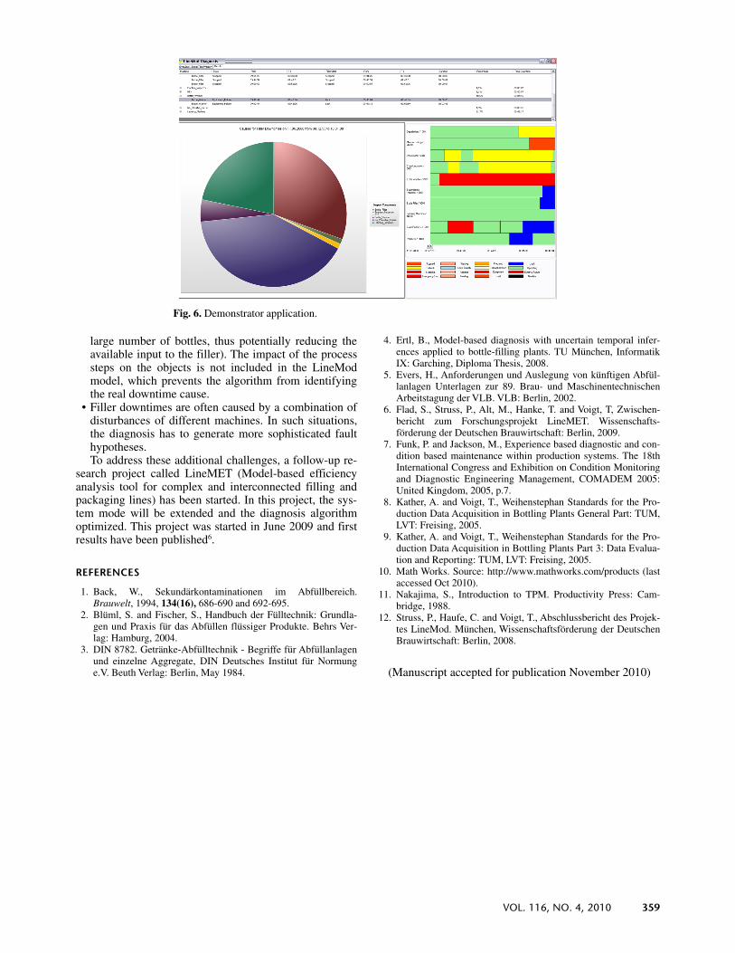
The model-based diagnosis algorithm was imple-mented in a demonstrator application which allowed analysis of downtimes of a bottling plant. This was tested at the plants of industrial project partners. The diagnosis tool (Fig. 6) localizes the machines causing downtime of the filler within certain time periods, which can be speci-fied by the user. As practitioners approved, the achieved result supports plant operators and supervisors in identify-ing critical points of the bottling plant and in explaining downtime losses and some speed losses (Fig. 2).

The correctness of the diagnosis suffices to make it a useful tool in practice. Wrong diagnosis results were often caused by faults in the database, inexact manual down-time analysis or plant-specific critical points that were too difficult to find automatically (missing observation data for the specific problem).

LineMod exclusively considers reasons for filler down-times and only those within the plant and, thus, has a number of limitations as follows.

• LineMod focused on “hard” failures (stop of bottling filler) caused by hard faults, which can be based on distinguishing zero from non-zero flow only. For cap-turing “soft” faults (e.g., reduced output) which lead, perhaps in combination, to a hard failure or a subopti-mal behaviour, a different model is required.

• Many efficiency losses are not caused by technical components, but rather by logistic processes down-stream or upstream of the plant. To analyse such situa-tions, the plant model needs to be extended.

• Sometimes, machine downtimes could not be assigned to the actual cause, because a machine treated objects incorrectly (e.g., improper cleaning of dirty bottles). The effect of the defective treatment may become evi-dent only after some time period at another machine (e.g., the empty bottle inspector, which will reject a

Table II. Experimental validation of the diagnosis correctness.

Experimentation day

6/10/2008 6/11/2008 9/28/2008 9/29/2008 Sum Percent

Downtime Caused by filler 109 22 86 39 256 Lack 34 5 57 26 122 Tailback 21 2 7 7 37

All cases Model based diagnosis compliance 160 28 140 69 397 96%

no compliance 4 1 10 3 18 04% Non trivial cases compliance 51 6 54 30 141 89% no compliance 4 1 10 3 18 11%

VOL. 116, NO. 4, 2010 359

large number of bottles, thus potentially reducing the available input to the filler). The impact of the process steps on the objects is not included in the LineMod model, which prevents the algorithm from identifying the real downtime cause.

• Filler downtimes are often caused by a combination of disturbances of different machines. In such situations, the diagnosis has to generate more sophisticated fault hypotheses. To address these additional challenges, a follow-up re-

search project called LineMET (Model-based efficiency analysis tool for complex and interconnected filling and packaging lines) has been started. In this project, the sys-tem mode will be extended and the diagnosis algorithm optimized. This project was started in June 2009 and first results have been published6.

REFERENCES

1. Back, W., Sekundärkontaminationen im Abfüllbereich. Brauwelt, 1994, 134(16), 686-690 and 692-695.

2. Blüml, S. and Fischer, S., Handbuch der Fülltechnik: Grundla-gen und Praxis für das Abfüllen flüssiger Produkte. Behrs Ver-lag: Hamburg, 2004.

3. DIN 8782. Getränke-Abfülltechnik - Begriffe für Abfüllanlagen und einzelne Aggregate, DIN Deutsches Institut für Normung e.V. Beuth Verlag: Berlin, May 1984.

4. Ertl, B., Model-based diagnosis with uncertain temporal infer-ences applied to bottle-filling plants. TU München, Informatik IX: Garching, Diploma Thesis, 2008.

5. Evers, H., Anforderungen und Auslegung von künftigen Abfül-lanlagen Unterlagen zur 89. Brau- und Maschinentechnischen Arbeitstagung der VLB. VLB: Berlin, 2002.

6. Flad, S., Struss, P., Alt, M., Hanke, T. and Voigt, T, Zwischen-bericht zum Forschungsprojekt LineMET. Wissenschafts-förderung der Deutschen Brauwirtschaft: Berlin, 2009.

7. Funk, P. and Jackson, M., Experience based diagnostic and con-dition based maintenance within production systems. The 18th International Congress and Exhibition on Condition Monitoring and Diagnostic Engineering Management, COMADEM 2005: United Kingdom, 2005, p.7.

8. Kather, A. and Voigt, T., Weihenstephan Standards for the Pro-duction Data Acquisition in Bottling Plants General Part: TUM, LVT: Freising, 2005.

9. Kather, A. and Voigt, T., Weihenstephan Standards for the Pro-duction Data Acquisition in Bottling Plants Part 3: Data Evalua-tion and Reporting: TUM, LVT: Freising, 2005.

10. Math Works. Source: http://www.mathworks.com/products (last accessed Oct 2010).

11. Nakajima, S., Introduction to TPM. Productivity Press: Cam-bridge, 1988.

12. Struss, P., Haufe, C. and Voigt, T., Abschlussbericht des Projek-tes LineMod. München, Wissenschaftsförderung der Deutschen Brauwirtschaft: Berlin, 2008.

(Manuscript accepted for publication November 2010)

Fig. 6. Demonstrator application.