automated tracking and grasping of a moving object with a

152 IEEE TRANSACTIONS ON ROBOTICS AND AUTOMATION, VOL. 9, NO. 2, APRIL 1993

Automated Tracking and Grasping of a Moving Object with a Robotic Hand-Eye System

Peter K. Allen, Member, IEEE, Aleksandar Timcenko, Student Member, IEEE, Billibon Yoshimi, Student Member, IEEE, and Paul Michelman, Member, IEEE

Abstract- Most robotic grasping tasks assume a stationary or fixed object. In this paper, we explore the requirements for tracking and grasping a moving object. The focus of our work is to achieve a high level of interaction between a real-time vision system capable of tracking moving objects in 3-D and a robot arm with gripper that can be used to pick up a moving object. There is an interest in exploring the interplay of hand-eye coordination for dynamic grasping tasks such as grasping of parts on a moving conveyor system, assembly of articulated parts, or for grasping from a mobile robotic system. Coordination between an organism's sensing modalities and motor control system is a hallmark of intelligent behavior, and we are pursuing the goal of building an integrated sensing and actuation system that can operate in dynamic as opposed to static environments. The system we have built addresses three distinct problems in robotic hand-eye coordination for grasping moving objects: fast computation of 3-D motion parameters from vision, predictive control of a moving robotic arm to track a moving object, and interception and grasping. The system is able to operate at approximately human arm movement rates, and experimental results in which a moving model train is tracked is presented, stably grasped, and picked up by the system. The algorithms we have developed that relate sensing to actuation are quite general and applicable to a variety of complex robotic tasks that require visual feedback for arm and hand control.

I. INTRODUCTION

HE focus of our work is to achieve a high level of T interaction between a real-time vision system capable of tracking moving objects in 3-D and a robot arm equipped with a dextrous hand that can be used to intercept, grasp, and pick up a moving object. We are interested in exploring the interplay of hand-eye coordination for dynamic grasping tasks such as grasping of parts on a moving conveyor system, assembly of articulated parts, or for grasping from a mobile robotic system. Coordination between an organism's sensing modalities and motor control system is a hallmark of intelligent behavior, and we are pursuing the goal of building an integrated sensing and actuation system that can operate in dynamic as opposed to static environments.

There has been much research in robotics over the last few years that addresses either visual tracking of moving objects or generalized grasping problems. However, there have been

Manuscript received October 14, 1991; revised June 2, 1992. This work was supported in part by DARPA under Contract "39-84-C-0165, by NSF under Grants DMC-86-05065, DCI-86-08845, CCR-86.12709, IRI-86- 57151, and IRI-88-1319 by North American Philips Laboratories, by Siemens Corporation, and by Rockwell Inc.

The authors are with the Department of Computer Science, Columbia University, New York, NY 10027.

IEEE Log Number 9207358.

few efforts that try to link the two problems. It is quite clear that complex robotic tasks such as automated assembly will need to have integrated systems that use visual feedback to plan, execute, and monitor grasping.

The system we have built addresses three distinct problems in robotic hand%ye coordination for grasping moving objects: fast computation of 3-D motion parameters from vision, predictive control of a moving robotic arm to track a moving object, and interception and grasping. The system is able to operate at approximately human arm movement rates, using visual feedback to track, intercept, stably grasp, and pick up a moving object. The algorithms we have developed that relate sensing to actuation are quite general and applicable to a variety of complex robotic tasks that require visual feedback for arm and hand control.

Our work also addresses a very fundamental and lim- iting problem that is inherent in building integrated sensing/actuation systems; integration of systems with different sampling and processing rates. Most complex robotic systems are actually amalgams of different processing devices, con- nected by a variety of methods. For example, our system consists of three separate computation systems: a parallel image processing computer; a host computer that filters, trian- gulates, and predicts 3-D position from the raw vision data; and a separate arm control system computer that performs inverse kinematic transformations and joint-level servoing. Each of these systems has its own sampling rate, noise characteristics, and processing delays, which need to be integrated to achieve smooth and stable real-time performance. In our case, this involves overcoming visual processing noise and delays with a predictive filter based upon a probabilistic analysis of the system noise characteristics. In addition, real-time arm control needs to be able to operate at fast servo rates regardless of whether new predictions of object position are available.

The system consists of two fixed cameras that can image a scene containing a moving object (Fig. 1). A PUMA-560 with a parallel jaw gripper attached is used to track and pick up the object as it moves (Fig. 2) . The system operates as follows:

1) The imaging system performs a stereoscopic optic-flow calculation at each pixel in the image. From these optic- flow fields, a motion energy profile is obtained that forms the basis for a triangulation that can recover the 3-D position of a moving object at video rates.

2) The 3-D position of the moving object computed by step 1 is initially smoothed to remove sensor noise, and a nonlinear filter is used to recover the correct

1042-296X/93$03.00 0 1993 IEEE

I

153 ALLEN et al.: AUTOMATED TRACKING AND GRASPING OF A MOVING OBJECT

\ circie of radius 250 millimeters

L Stereo J Cameras

Fig. 1 . Tracking/grasping system.

trajectory parameters which can be used for forward prediction, and the updated position is sent to the trajectory- planner/arm-control system.

3) The trajectory planner updates the joint-level servos of the arm via kinematic transform equations. An additional fixed-gain filter is used to provide servo-level control in case of missed or delayed communication from the vision and filtering system.

4) Once tracking is stable, the system commands the arm to intercept the moving object and the hand is used to grasp the object stably and pick it up.

The following sections of the paper describe each of these subsystems in detail along with experimental results.

11. PREVIOUS WORK Previous efforts in the areas of motion tracking and real-

time control are too numerous to exhaustively list here. We instead list some notable efforts that have inspired us to use similar approaches. Burt et al. [9] have focused on high- speed feature detection and hierarchical scaling of images in order to meet the real-time demands of surveillance and other robotic applications. Related work has been reported by Lee and Wohn [29] and Wiklund and Granlund [43] who use image differencing methods to track motion. Corke, Paul, and Wohn [13] report a feature-based tracking method that uses special-purpose hardware to drive a servo controller of an arm-mounted camera. Goldenberg et al. [ 161 have developed a method that uses temporal filtering with vision hardware similar to our own. Luo, Mullen, and Wessel [30] report a real- time implementation of motion tracking in 1-D based on Horn and Schunk’s method. Verghese et ul. [41] report real-time short-range visual tracking of objects using a pipelined system similar to our own. Safadi [37] uses a tracking filter similar to our own and a pyramid-based vision system, but few results are reported with this system. Rao and Durrant-Whyte [36] have implemented a Kalman filter-based decentralized tracking

Fig. 2 . Experimental hardware

system that tracks moving objects with multiple cameras. Miller [31] has integrated a camera and arm for a tracking task where the emphasis is on learning kinematic and control parameters of the system. Weiss et al. [42] also use visual feedback to develop control laws for manipulation. Brown [8] has implemented a gaze control system that links a robotic “head” containing binocular cameras with a servo controller that allows one to maintain a fixed gaze on a moving object. Clark and Ferrier [12] also have implemented a gaze control system for a mobile robot. A variation of the tracking problems is the case of moving cameras. Some of the papers addressing this interesting problem are 191, [15], [441, and [18].

The majority of literature on the control problems encoun- tered in motion tracking experiments is concerned with the problem of generating smooth, up-to-date trajectories from noisy and delayed outputs from different vision algorithms. Our previous work [4] coped with that problem in a similar way as in [38], using an cy - p - y filter, which is a form of steady-state Kalman filter. Other approaches can be found in papers by [33], [34], [28], [6]. In the work of Papanikolopoulos et al. [33], [34], visual sensors are used in the feedback loop to perform adaptive robotic visual tracking. Sophisticated control schemes are described which combine a Kalman filter’s estimation and filtering power with an optimal (LQG) controller which computes the robot’s motion. The vision system uses an optic-flow computation based on the SSD (sum of squared differences) method which, while time consuming, appears to be accurate enough for the tracking


task. Efficient use of windows in the image can improve the performance of this method. The authors have presented good tracking results, as well as stated that the controller is robust enough so the use of more complex (time-varying LQG) methods is not justified. Experimental results with the CMU Direct Drive Arm I1 show that the methods are quite accurate, robust, and promising.

The work of Lee and Kay [28] addresses the problem of uncertainty of cameras in the robot’s coordinate frame. The fact that cameras have to be strictly fixed in robot’s frame might be quite annoying since each time they are (most often incidentally) displaced, one has to undertake a tedious job of their recalibration. Again, the estimation of the moving object’s position and orientation is done in the Cartesian space and a simple error model is assumed. Andersen et al. [6] adopt a 3rd-order Kalman filter in order to allow a robotic system (consisting of two degrees of freedom) to play the labyrinth game. A somewhat different approach has been explored in the work of Houshangi [24] and Koivo et al. [27]. In these works, the autoregressive (AR) and autogressive moving-average with exogenous input (ARMAX) models are investigated for visual tracking.

111. VISION SYSTEM

In a visual tracking problem, motion in the imaging system has to be translated into 3-D scene motion. Our approach is to initially compute local optic-flow fields that measure image velocity at each pixel in the image. A variety of techniques for computing optic-flow fields have been used with varying results including matching-based techniques [5], [ 101, [39], gradient-based techniques [23], [32], [ 113, and spatio- temporal energy methods [20], [2]. Optic-flow was chosen as the primitive upon which to base the tracking algorithm for the following reasons.

The ability to track an object in three dimensions implies that there will be motion across the retinas (image planes) that are imaging the scene. By identifying this motion in each camera, we can begin to find the actual 3-D motion. The principal constraint in the imaging process is high computational speed to satisfy the update process for the robotic arm parameters. Hence, we needed to be able to compute image motion quickly and robustly. The Hom-Schunck optic-flow algorithm (described below) is well suited for real-time computation on our PIPE image processing engine. We have developed a new framework for computing optic-flow robustly using an estimation-theoretic framework [40]. While this work does not specifically use these ideas, we have future plans to try to adapt this algorithm to such a framework.

Our method begins with an implementation of the Horn-Schunck method of computing optic-flow [22]. The underlying assumption of this method is the optic-flow constraint equation, which assumes image irradiance at time t and t + S t will be the same:

I ( z + sz, y + sy, t + S t ) = I(2, y, t ) . (1)

If we expand this constraint via a Taylor series expansion, and drop second- and higher-order terms, we obtain the form of the constraint we need to compute normal velocity:

where U and U are the velocities in image space, and I,, IY, and 1, are the spatial and temporal derivatives in the image. This constraint limits the velocity field in an image to lie on a straight line in velocity space. The actual velocity cannot be determined directly from this constraint due to the aperture problem, but one can recover the component of velocity normal to this constraint line as

A second, iterative process is usually employed to propagate velocities in image neighborhoods, based upon a variety of smoothness and heuristic constraints. These added neighbor- hood constraints allow for recovery of the actual velocities U ,

U in the image. While computationally appealing, this method of determining optic-flow has some inherent problems. First, the computation is done on a pixel-by-pixel basis, creating a large computational demand. Second, the information on optic flow is only available in areas where the gradients defined above exist.

We have overcome the first of these problems by using the PIPE image processor [26], [7]. The PIPE is a pipelined parallel image processing computer capable of processing 256 x 256 x 8 bit images at frame rate speeds, and it supports the operations necessary for optic-flow computation in a pixel- parallel method (a typical image operation such as convolution, warping, additionkubtraction of images can be done in one cycle-l/60 s). The second problem is alleviated by our not needing to know the actual velocities in the image. What we need is the ability to locate and quantify gross image motion robustly. This rules out simple differencing methods which are too prone to noise and will make location of image movement difficult. Hence, a set of normal velocities at strong gradients is adequate for our task, precluding the need to iteratively propagate velocities in the image.

A. Computing Normal Optic-Flow in Real-Time

Our goal is to track a single moving object in real time. We are using two fixed cameras that image the scene and need to report motion in 3-D to a robotic arm control program. Each camera is calibrated with the 3-D scene, but there is no explicit need to use registered (i.e., scan-line coherence) cameras. Our method computes the normal component of optic-flow for each pixel in each camera image, finds a centroid of motion energy for each image, and then uses triangulation to intersect the back-projected centroids of image motion in each camera. Four processors are used in parallel on the PIPE. The processors are assigned as four per camera-two each for the calculation of X and Y motion energy centroids in each image. We also use a special processor board (ISMAP) to perform real-time

ALLEN et al.: AUTOMATED TRACKNG AND GRASPING OF A MOVING OBJECT 155

Gaussian

Fig. 3. PIPE motion tracking algorithm.

histogramming. The steps below correspond to the numbers in Fig. 3.

The camera images the scene and the image is sent to processing stages in the PIPE. The image is smoothed by convolution with a Gauss- ian mask. The convolution operator is a built-in operation in the PIPE and it can be performed in one frame cycle. In the next two cycles, two more images are read in, smoothed and buffered, yielding smoothed images Io and I1 and 12. The ability to buffer and pipeline images allows temporal operations on images, albeit at the cost of processing delays (lags) on output. There are now three smoothed images in the PIPE, with the oldest image lagging by 3/60 s. Images Io and I , are subtracted yielding the temporal derivative I t . In parallel with step 5, image 11 is convolved with a 3 x 3 horizontal spatial gradient operator, returning the discrete form of I,. In parallel, the vertical spatial gradient is calculated yielding I, (not shown). The results from steps 5 and 6 are held in buffers and then are input to a look-up table that divides the temporal gradient at each pixel by the absolute value of the summed horizontal and vertical spatial gradients [which approximates the denominator in (3)]. This yields the normal velocity in the image at each pixel. These velocities are then thresholded and any isolated (i.e., single pixel motion energy) blobs are morphologically eroded. The above threshold velocities are then encoded as gray value 255. In our experiments, we thresholded all velocities below 10 pixels per 60 ms to zero velocity.

9-10) In order to get the centroid of the motion information, we need the X and Y coordinates of the motion energy. For simplicity, we show only the situation for the X coordinate. The gray-value ramp in Fig. 3 is an image that encodes the horizontal coordinate value (0-255) for each point in the image as a gray value. Thus, it is an image that is black (0) at horizontal pixel 0 and white (255) at horizontal pixel 255. If we logically and each pixel of the above threshold velocity image with the ramp image, we have an image which encodes high velocity pixels with their positional coordinates in the image, and leaves pixels with no motion at zero. By taking this result and histogramming it, via a special stage of the PIPE which performs histograms at frame rate speeds, we can find the centroid of the moving object by finding the mean of the resulting histogram. Histogramming the high-velocity position encoded images yields 256 16-bit values (a result for each intensity in the image). These 256 values can be read off the PIPE via a parallel interface in about 10 ms. This operation is performed in parallel to find the moving object’s Y centroid (and in parallel for X and Y centroids for camera 2). The total associated delay time for finding the centroid of a moving object becomes 15 cycles or 0.25 s.

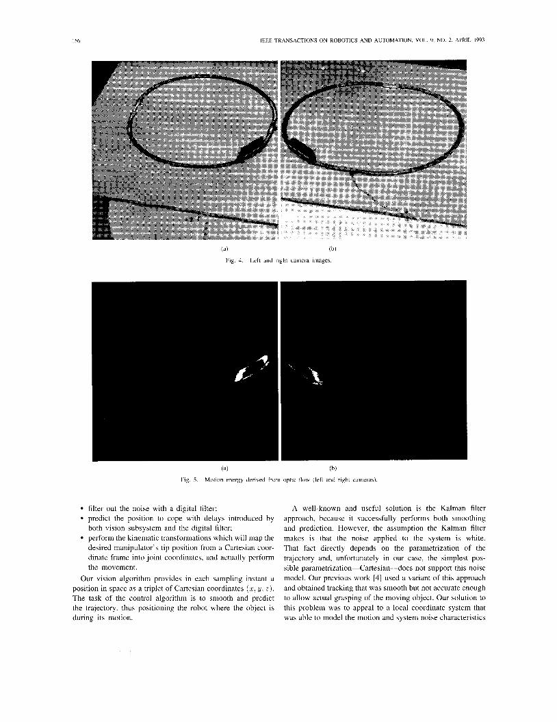
The same algorithm is run in parallel on the PIPE for the second camera. Once the motion centroids are known for each camera, they are back-projected into the scene using the camera calibration matrices and triangulated to find the actual 3-D location of the movement. Because of the pipelined nature of the PIPE, a new X or Y coordinate is produced every 1/60 s with this delay. Fig. 4 shows two camera images of a moving train, and Fig. 5 shows the motion energy derived from the real-time optic-flow algorithm.

While we are able to derive 3-D position from motion- stereo at real-time rates, there are a number of sources of noise and error inherent in the vision system. These include stereo- triangulation error, moving shadow s which are interpreted as object motion (we use no special lighting in the scene), and small shifts in centroid alignments due to the different viewing angles of the cameras, which have a large baseline. The net effect of this is to create a 3-D position signal that is accurate enough for gross-level object tracking, but is not sufficient for the smooth and highly accurate tracking required for grasping the object. We describe in the next section how a probabilistic model of the motion that includes noise can be used to extract a more stable and accurate 3-D position signal.

11)

IV. ROBOTIC ARM CONTROL

The second part of the system is the arm control. The robotic arm has to be controlled in real time to follow the motion of the object, using the output of the vision system. The raw vision system output is not sufficient as a control parameter since its output is both noisy and delayed in time. The control system needs to do the following:


(a) (b)

Fig. 4. Left and right camera images.

(a) (b)

Fig. 5 . Motion energy derived from optic flow (left and right cameras)

filter out the noise with a digital filter; predict the position to cope with delays introduced by both vision subsystem and the digital filter; perform the kinematic transformations which will map the desired manipulator’s tip position from a Cartesian coordinate frame into joint coordinates, and actually perform the movement.

Our vision algorithm provides in each sampling instant a position in space as a triplet of Cartesian coordinates ( x . y. z ) . The task of the control algorithm is to smooth and predict the trajectory, thus positioning the robot where the object is during its motion.

A well-known and useful solution is the Kalman filter approach, because it successfully performs both smoothing and prediction. However, the assumption the Kalman filter makes is that the noise applied to the system is white. That fact directly depends on the parametrization of the trajectory and, unfortunately in our case, the simplest pas- sible parametrization-Cartesian-does not support this noise model. Our previous work [4] used a variant of this approach and obtained tracking that was smooth but not accurate enough to allow actual grasping of the moving object. Our solution to this problem was to appeal to a local coordinate system that was able to model the motion and system noise characteristics

ALLEN et al.: AUTOMATED TRACKING AND GRASPING OF A MOVING OBJECT 157

no. of points

,,,o{ I

Fig. 6. Model of the motion in the plane: the moving object is in p k + l . while the vision system computes Q k f l . SO is the actual arc length, and s is the measured arc length.

Fig. 7. Experimental density of SI, the expected value of the arc length.

more accurately, thus producing a more accurate control algorithm.

A. The Model of the Motion The model of the motion we are using separates 3-D space

into an X Y plane and the Z axis, and addresses these two components of motion separately. In the experimental results we present in Section VI, we have used the model to track planar trajectories. However, we still need to track the Z dimension to determine the height above the plane of the motion to command the robotic arm to correctly grasp the object. The tracking of the object in the X Y plane is done using a local model presented below, while the tracking in 2 is done with a Cartesian displacement using the fixed-gain filter described in [4].

The main idea in the trajectory parametrization used in this paper is to describe a point in a local coordinate frame, relative to the point from the previous sampling instant, by the triplet of coordinates (SO, $0, Az) where (see Fig. 6)

SO is the length of an arc between two points (we will approximate the arc length by a straight line section and set SO to be the distance between points and Pk+l,

SO = 11Pk+1-pkII where 1 1 . 1 1 denotes Euclidean distance); $0 is the “bending” of the trajectory; AZ is the altitude difference between two consecutive points.

Due to the existence of noise, the measured coordinates will be random variables with certain distributions. We have made the following assumptions, as a result of both reasoning about the vision algorithm and certain necessary simplifications.

In sampling instant k, our object is at point Pk. In the next sampling instant k + 1, the object is at Pk+1

and the point returned by the vision algorithm is &k+l.

The measured arc length is s = ll&k+l - 911. Q k f l is normally distributed around Pk+1. The noise can be expressed by its two components, tangential nt and normal n,, where both nt and n, are random variables. nt and n, are both zero-mean, with the same variance CT and mutually not correlated. Experimentally, it has been determined that their coefficient of correlation is between 0.1 and 0.2. AZ is independent of SO and $0 (i.e., the altitude Z is independent of the position in X Y plane).

This last assumption limits the method to tracking planar trajectories in space. However, the probabilistic method described below can be extended to arbitrary 3-D space curve trajectories by finding a distribution that will allow computation of a space curve torsion parameter. This essentially means creating a full Frenet Frame representation at each point in time.

Under these assumptions, it can be shown that (see Appen- dix I) the velocity ‘U and curvature K are

‘U = lim so/T (4)

K = lim tan 40/so ( 5 )

where SO = 114+1 - Pk11,$0 = 7r - LPk_1PkPk+l and T is the sampling interval.

Our model assumes the following coordinate transformation that relates the moving object’s coordinate frame at one instant with the next instant in time:

TA = rot(z, $0) o trans(z, so) o trans(z, Az) (6)

where rot and trans are rotation about and translation along a given axis. Presented as a 4 x 4 matrix, transformation (6) is

cos $0 -sin $0 0 SO cos $0

sin $0 cos $0 0 so sin $0

T A = [ 0 ~ A z . 0 0 0 1

What are the advantages of such a parametrization? The most obvious one is the simplicity of the prediction task in this framework; all we need is to multiply the velocity ‘U = so/T by the time T > I’ we want to predict, as well as “bending” $0. The next advantage is that in order to achieve an accurate prediction, we do not need a high-order model with the mostly heuristic tuning of numerous parameters. The price we have to pay is that Jiltering is not straightforward. It turns out that we cannot just apply a low-pass filter in order to recover a dc component from s, but rather we need a more elaborate approach that takes into account a probabilistic distribution of s. Fig. 7 is a histogram of the experimentally measured density of the computed arc length between triangulated image motion points. This distribution shows the need to use a more sophisticated method than a simple averaging filter, which we have found to be incorrect in being able to correctly estimate the movement of the object between vision samples.

T+O

T-0

] (7)

~


s = [J&k+i - pkll low pass filter (computed arc length including noise) r 3 c >

< V i S -;\; see section N.B)

(stt N.c)

nonlinear transform

r I

s2 (computed square ofthe arc length including noise)

low pass filta (sec section I V . 9

Fig. 8. Overview of the filtering method.

The analysis below describes a probabilistic model of the experimental distribution in Fig. 7, allowing us to recover the actual arc length parameter SO and the bending angle $0

at each sampling instant. While this model introduces more complexity than a standard Cartesian model, we will see below that it is more effective in allowing us to accurately predict and smooth our trajectory.

B. Estimating Arc Length SO and Bending Parameter $0

We begin this subsection with an intuitive overview of the method used to recover the actual arc length SO and actual bending parameter $0 from the noisy estimates provided by the vision system. The filtering method is summarized in Fig. 8. Given the model of the motion described in the previous subsection, we want to extract the actual arc length SO from measured, noisy arc length s. Using a smoothing filter (see subsection C), we can derive the expected value of the arc length which we denote S I , as well as its second-order moment (expectation of s2) which we denote sz. These two control inputs, s1 and sz, can be used to create two integral equations [(13) and (15)] which, when integrated, express the known smoothed control inputs s1 and sg as functions of the actual arc length SO and a variance 0. These equations allow us to estimate SO from the control inputs. To recover the actual bending parameter $ 0 , our task is simplified since its distribution is symmetric, and its expectation is the actual bending parameter itself.

Let s = l IQk+l - Pkll be the distance between the object and the next position returned by the vision algorithm. Let 3 k be the moving coordinate frame of the point Pk with axes t , n, and 2, where t is the tangential and n normal to the trajectory’s projection in X Y plane (see Fig. 6) , and let 3 k + l

be the analogous coordinate frame in the point Pk+1. The transformation from 3 k to 3 k + 1 is given by TA:

The point Q k + l is given by 3 k + 1 by a triple (nt ,n, ,z) , where nt is a noise component along t , and n, is a noise component along n. Both nt and n, are Gaussian with zero mean and mutually noncorrelated. Coordinate z is the altitude at p k + 1 .

In the coordinate frame 3 k , the point Qk+l is given by !!‘il[nt n, z 1IT. Thus, the distance s = I lQk+l - 911 is given by

where n: = nt cos $0 + n, sin 40 and n’, = -nt sin $0 + n, cos $0. n: and n’, are obtained by “rotating” nt and n, by $0. It is known that the transformation of noiicorrelated Gaussian random variables results in noncorrelated Gaussian random variables with the same variance. Thus, n: and n’, are noncorrelated and Gaussian with the variance 0.

Now we have expressed in relation (8) the dependency of s on two random variables with known properties n: and n’,. The formula for random variables’ distribution transformations gives us the distribution function F ( s ) . (Note that henceforth s is used to denote the argument of the distribution or distribution density functions.)

where D is a disk of radius s about 4. We need to find the expectation of the random variable

whose distribution is given by (9). In order to do that, we need the density function which can be found by calculating the integral in (9). By introducing the substitution t = r cos B,n = r sin 0, we get

The distribution density is given as f ( s ) = differentiation,

or, after

The last integral can be expressed by a modified Bessel function Io ( z )

ALLEN et al.: AUTOMATED TRACKING AND GRASPING OF A MOVING OBJECT 159

2 3 4

Fig. 10. y = ui(z) .

Fig. 9. Distribution density f ( s ) , s o = 1,a = 0.4-1.0, incremenr = 0.1.

A graph of f(s) is given in Fig. 9. Here, SO is fixed to 1, and r~ varies from 0.4 to 1.0. Our job is to recover SO given f(s).

It is apparent from Fig. 9 that the peak value of f (s) depends on o, and drifts toward higher values as o grows. The expectation for s also depends on 0. In particular, we have

where -

U(.) = -x2/4 Fig. 1 1 . Distribution density f ( 4 ) . &e

. ( l o ( : ) 4- :(Io(:) +11(:))).(14) o = s2 (19) 1

Here, r~ is the constant for the given system and it is related Jq$ to SO. In order to estimate o, we will use the second-order moment This method requires little on-line computation-an inter-

polation table of values of u1 is all we need to recover the

To find the bending parameter $0, we use the same tech- nique as for the distribution of s, and we get the following formula:

00 si E(s2 ) = / s2f(s)ds = + 2a2’ (15) arc length parameter so.

Equations (13) and (15) are derived in Appendix 11. Now by eliminating SO from (13) and (15), we have

l=zu( @T@ ) where p = sz/s1 and z = o / s l . Now by setting x =

L , we end up with an equation (see Appendix 111) F where k = o/So and $ - $0 E (-r/’,&r/2). It is obvious that f is symmetric around $0, which also means that the expectation E$ = $0. Hence, we so not need to perform a nonlinear filtering to recover $0.

The graph of f for k = 0.1 to 0.9 and $0 = 0 is given in Fig. 11.

= p . (17)

Equation (17) relates our known control inputs ( p = s2/s1)

dZ-5 Ul(X) = ___ 4.)

to x. We can create a table of values for this function off line, and then by interpolation calculate a value of x given p .

Let x~(p) be the solution of (17). Now we can express SO and o as functions of SI and s2 as follows:

c. Smoothing of the Control Inputs

In the previous subsection, we showed how to extract parameters SO and $0 from the updated positions determined from the vision system. The signals ~1,s: described in (13) and (15) are in fact the smoothed versionsbf the expectations of the control signals s, s2 which are the arc length and the arc length squared. The smoothing filter we use to compute these signals is a moving-average (MA) filter using a Kaiser window [25]. This filter provides the largest ratio of signal

(18) so = s:,


Tool

S

1 Bare Obj Grasp 1 w- 0

Graph nodes represent coordinate frames:

W is world-coordinate frame

S is robot shoulder coordinate frame

M is 6th joint coordinate frame

T is tool (gripper) coordinate frame

G is grasping position coordinate frame

0 is moving object coordinate frame

Graph edges represent 4 x 4 coordinate transforms:

Bare is constant transform between W and S

T6 is variable transform computed by RCCL in each sampling interval

Tool IS variable transform defined by the hand kinematics

Drive is the transform introduced internally by RCCL to obtain straight-line motion in Carte-

sian coordinates

Grasp is constant transform which defines grasping point relative to the moving abject

Obj is variable transform defined by vision subsystem outputs - it defines the position of the

moving object in the world coordinate frame

Fig. 12. Transform equation.

energy in the main lobe and a side lobe, which usually results in a filter of lower order. The windowing function is given by

where Io is the modified zeroth-order Bessel function, ,B is the shape parameter which defines the width of the main lobe, and M is the order of the filter. According to [25], ,B and M are given by

. . A - 7.95 ME-----

14.36Aw and

0.1102(A - 8.7), A 2 50 ,B={ 0.5842(A - 21)0.4 + 0.07886(A - 21), 21 < A < 50

where A is the stopband attenuation and Aw = (wr - w,)/ws, wr is the stopband frequency, w, is the passband frequency, and w, is the sampling frequency.

We have adopted A = 30 and Aw = 0.05 which results in M = 30. Since the frequency of the vision algorithm is about 60 Hz, the overall length of the window is about 0.5 s. We also apply this MA filter to the bending parameter 4.

The implementation of MA filter is straightforward: once the weights are computed off line, a window of length M of measurements is retained and each sample is multiplied by an appropriate weight in the sampling period, which requires M

multiplications and M - 1 additions. This allows reasonably wide windows (even up to several hundred entries) to be used in computing the smoothed signal.

D. Prediction and Synchronization

The host computer controls the initial vision processing and subsequent computation of control parameters described above. The host computer is able to predict the trajectory using the derivation of velocity and curvature in (4) and (5). These updated predictions are sent to the trajectory generator that is actually controlling the robot arm. The trajectory generator is a separate system that has two parallel tasks: a low- priority task which reads the serial line receiving updated control signals, and a high-priority task which calculates the transformation equation and moves the manipulator. Those two tasks communicate via shared memory. The job of the robot controlling program is to synchronize its two tasks (i.e., to obtain mutual exclusion in accessing shared data), to unpack input packets read from the serial line, and to update the joint servos every 30 ms.

The asynchronous nature of the communication between the host computer and the trajectory generator can result in missed or delayed communications between the two systems. Since the updating of the robotic arm parameters needs to be done at very tightly specified servo rates (30 ms), it is imperative that the trajectory generator can provide updated control parameters at these rates, regardless of whether it has received a new control input from the host. Therefore, we have implemented a fixed-gain LY - ,B - y filter as part of the trajectory generator [38]. This filter provides a small amount of prediction to the trajectory parameters if the control signals from the host are delayed.

We are using RCCL [19] to control the robotic arm (a PUMA 560). RCCL (Robot Control C Language) allows the use of C programming constructs to control the robot as well as defining transformation equations (as described in [35]). The transformation equations permit dynamic updating of arm position by generating the 4 x 4 transform of the moving object’s position from the vision system and sending this information to the arm control algorithm (see Fig. 12).

v. MOTOR COORDINATION FOR GRASPING

The remaining part of our system is the interception and grasping of the object. This is the least well-developed aspect of our system, since it is a difficult real-time problem. Cur- rently, we are intercepting and grasping a simple object with no knowledge of its local geometry. In the future, we hope to use visual information as well finger contact information to perform grasping of objects of different shapes.

We have examined the human psychological literature in order to find useful paradigms for robotic visual-motor coordination strategies that include arm movement and grasping from visual inputs. Schmidt [I71 has proposed a theory of generalized motor programs, or movement schemas. In this view, a skilled action is composed of an ordered set of parametrized motor control programs of short duration (less than 200 ms), each of which accomplishes one part of the task. As one program is completed, the next one is executed. At the

ALLEN et al.: AUTOMATED TRACKING AND GRASPING OF A MOVING OBJECT

~

161

initiation of a skilled task, the parameters of the motor control program are determined by sensory input and task demands, and then the programs are executed to completion. If the wrong program is selected for some reason, the program cannot be stopped by use of sensory information. An example of this can be seen in the motor activity associated with playing table tennis. In moving the arm to hit the ball, the motion of the racket is determined before the beginning of the swing and visual input has little effect after the initiation of motion. As an example of Schmidt’s theory, the skilled task of grasping a moving object could be partitioned into two motor control schemas: one to position the arm and a second one to control the grasping action.

The initial strategy we have adopted in picking up the object is an open-loop strategy, similar in spirit to the preprogrammed motor control schemas described above. Schmidt’s schema theory holds that for tasks of short duration, perception is used to find a set of parameters to pass to a motor control program. It is not used during the execution of a task. When grasping a moving object, for example, once vision has determined the trajectory of the object, the reach and grasping motor schemas take over with no interference from vision. Recent work described in [21] suggests that visual input may be used to modify human arm grasping trajectories, but only after a 100 ms or more delay after receiving the visual input. Since our visual inputs are already delayed by this amount, it may not be possible to use our current vision system effectively in this part of the task, motivating the use of open-loop schemas.

In our implementation of this strategy, vision is not used to continually monitor the grasping, but only to provide a final position and velocity from which the arm is directed to very quickly move to the object. This automatic movement is done by establishing coordinate frames of action for each of the components of the system and solving transformation equations (see Fig. 12).

The transformation equations permit dynamic updating of the arm position by generating the 4 x 4 transform of the moving object’s position from the vision system and sending this information to the arm control algorithm. This positional information from the vision system is used to update the Obj transform in Fig. 12. The other transforms in the equation are known, and this allows the system to solve for the Drive transform which is the transform used to update the manipulator’s joints and develop a straight line path in Cartesian coordinates that will bring the hand into contact with the moving object. Because the movement of the hand requires a small amount of time during which the object may have moved, the object’s trajectory is predicted ahead during the movement using the (Y - ,8 - y predictor. By keeping the fingers of the hand spread during this maneuver, no actual contact takes place until the gripper reaches the position of the moving object. Once this position is achieved, the gripper is commanded to close and grasp the object.

VI. EXPERIMENTAL RESULTS We have implemented the system described above in order

to demonstrate the capability of the methods. The goal was

”T

Fig. 13. Input signal s: (black) and filtered signal S O (gray). Horizontal axis is time expressed in sampling periods (1 unit = 20 ms) and vertical axis is arc length in millimeters.

to track a moving model train, intercept it, stably grasp it, and pick it up. The train was moving in an oval trajectory; however, the system had no a priori knowledge of this particular trajectory. The velocity of the train was varied from 10-30 c d s . We have experimentally established 100 ms to be the appropriate time to predict. Since the trajectory generation runs at 20 ms, that makes five sampling intervals. The accuracy of tracking was critical; in order not to knock the train off but rather to pick it up the displacement of the robot’s gripper from the actual train’s position has to be in subcentimeter range.

In this section we present some results obtained by experiments. First, in Fig. 13, we have the actual measured arc length signal SI (black) and the filtered signal SO (gray). It is noticeable that SO is somewhat below the expected value of SI. The nature of s1 is quite noisy; however, the analysis described in Section IV was able to accurately extract the correct control signal. The arm control is particularly smooth and jerk free, stable over time (the tracking is continuous for many revolutions of the train) and is highly accurate in being able to intercept and grasp the object between the jaws of the gripper as it moves. Fig. 17 shows the trajectory of commanded arm control set points in the zy plane, including the initial trajectory at system start. The actual train track is an oval, slightly tilted from the horizontal axis. As a part of a system, we have implemented a simple on-line graphic interface in X-windows environment. Fig. 18 shows the graphics window captured during an experiment. Positions are taken each 500 ms and plotted in the window. Figs. 14, 15, and 16 show the time dependency of the z, y, and z coordinates. The tail of Fig. 16 is part of the grasping trajectory.

Because we are using a parallel jaw gripper, the jaws must remain aligned with the tangent to the actual trajectory of the moving object. This tangential direction is computed directly from the calculation of the bending parameter 4 during the trajectory modeling phase and is used to align joint 6 of the robot to keep the gripper correctly aligned. This correct alignment allows grasping to occur at any point in the trajectory.

Fig. 19 shows three frames taken from a video tape of the system intercepting, grasping, and picking up the object. The system is quite repeatable, and is able to track other arbitrary


2m

L C a

Y ["I

.

t [sec]

-tm

-200

Fig. 18. Object trajectory in XY plane: on-line graphics window including Fig. 16. Z coordinate of the commanded arm control set points for the tracked trajectory as a function of time. The tail is the movement of the arm to effect the grasp of the object.

start-up points.

The system is robust in a number of ways. The vision system does not require special lighting, object structure, or reflectance properties to compute motion since it is based upon calculating optic-flow. The control system is able to cope with the inherent visual sensor noise and triangulation error by

trajectories in addition to the one shown. ne system is also capable of tracking motion direction reversals (with overshoot) if the train fonvard and then in reverse.

.

.

VII. SUMMARY AND FUTURE WORK

We have developed a robust system for tracking and grasping moving objects. The system relies on real-time stereo- triangulation of optic-flow and is able to cope with the inherent noise and inaccuracy of visual sensors by applying parameterized filters that smooth and can predict the moving object's position. Once this tracking is achieved, a grasping strategy is applied that performs an analog of human arm movement schemas.

using a probabilistic noise model and local parameterization that can be used to build a nonlinear filter to extract accurate control parameters. The arm control system is able to cope with the inherent bandwidth mismatches between the vision sampling rate and the servo-update rate by using a fixed- gain predictive filter that allows arm control to function in the occasional absence of a video control signal. Finally, the system is robust enough to repeatedly pick up a moving object and stably grasp it.

We are currently extending this system to other hand-eye coordination tasks. An extension we are pursuing is to im-

ALLEN et al.: AUTOMATED TRACKING AND GRASPING OF A MOVING OBJECT

Fig. 20. Trajectory curvature n.

(b)

Fig. 19. Intercepting (a), grasping (b), and picking up (c) the object.

plement other grasping strategies. One strategy is to visually monitor the interception of the hand and object and use this visual information to update the Drive transform at video update rates. This approach is computationally more demand- ing, requiring multiple moving object tracking capability. The initial vision tracking described above is capable of single object tracking only. If we attempt to visually servo the moving robotic arm with the moving object, we have introduced multiple moving objects into the scene.

~

163

We have identified two possible approaches to tracking these multiple objects visually. The first is to use the PIPE’S region of interest operator that can effectively “window” the visual field and compute different motion energies in each window concurrently. Each region can be assigned to a different stage of the PIPE and compute its result independently. This approach assumes that the moving objects can be segmented. This is possible since the motion of the hand in 3-D is known-we have commanded it ourselves. Therefore, since we know the camera parameters and 3-D position of the hand, it will be possible to find the relevant image-space coordinates that correspond to the 3-D position of the hand. Once these are known, we can form a window centered on this position in the PIPE, and concurrently compute motion energy of the moving object and the moving hand in each camera. Each of these motion centroids can then be triangulated to find the effective positions of both the hand and object and compute the new Drive transform. Both computations must, however, compete for the hardware histogramming capability needed for centroid computation, and this will effectively reduce the bandwidth of position updating by a factor of 2.

Another approach is to use a coarse-fine hierarchical control system that uses a multisensor approach. As we approach the object for grasping, we can shift the visual attention from the static cameras used in 3-D triangulation to a single camera mounted on the wrist of the robotic hand. Once we have determined that the moving object is in the field of view of this camera, we can use its estimates of motion via optic-flow to keep the object to grasped in the center of the wrist camera’s field of view. This control information will be used to compute the Drive transform to correctly move the hand to intercept the object. We have implemented such a tracking system with a different robotic system [3] and can adapt this method to this particular task.

APPENDIX I TRAJECTORY CURVATURE

Here we prove that the trajectory curvature is given by the formula K = 1imT-o tan ( P ~ / S O where the following nomenclature is being adopted (see Fig. 20):

K is the trajectory curvature. T is the sampling interval.

IEEE TRANSACTIONS ON ROBOTICS AND AUTOMATION, VOL. 9. NO. 2, APRIL 1993

P k - 1 , 9 , 9 + 1 are three consecutive points along the trajectory. SO = 11Pk+1 - 411 is the distance between points Pk+1

0 is the center of rotation. V k = LPk-lOPk is the angle between the tangent lines

Cpk = LPk-lOPk is the angle between the tangent lines

cpo = { v k + Vk+1}/2 is the angle between lines and PkPk+l.

$k is the angle which tangent line t k forms with the x axis.

and 4.

t k - 1 and t k .

t k - 1 and t k .

Now we have

d - tan cpo - lim - - lim

T+O sn T-+O ds dT tan PO

- dT

1 1 d $ k + l - $ k - l = - lim ~- v T+O cos2 cpo dT 2

1 d arctan yL+l - arctan yk-l 2

which is the formula for curvature [14].

APPENDIX I1 VELOCITY EXPECTATION AND VARIANCE

In order to compute the mathematical expectation of the velocity, we differentiate the following integral (integral l l .4.3 l in [l]):

with respect to a, and by setting a = 1/2a2, b = so/a2, we get formula (13).

To prove formula (15) we use formula (11.4.29) from [ l ] (we set v = 0):

@/4a

e-at2tIo(bt)dt = - (B2) 2a .

By differentiation with respect to a, and introducing the substitutions for a and b as in (21), we get the formula (15).

APPENDIX I11

Formula (17) follows from (16) as follows: from x = J m / z , we get by solving for z : z = p / d m . After substituting the value for z into (16), (17) follows immediately.

Since x = J?;2-zFz/z = d m / a , after solving for a we get a = s2/dm, which is equivalent to (19). From (15) it follows that SO = Jm. By substituting the value for o, we get SO = Js; - 2s:/(zg + 2). It is easily shown that the last expression is equivalent to (1 8).

VERIFICATION OF FORMULAS (17), (18), AND (19)

REFERENCES

M. Abramowitz, Ed., Handbook of Mathematical Functions, National Bureau of Standards, 1964. E. H. Adelson and J. R. Bergen, “Spatio-temporal energy models for the perception of motion,” J. Opt. Soc. Amer., vol. 2, no. 2, pp. 284-299, 1985. P. Allen, “Real-time motion tracking using spatio-temporal filters,” in Proc. DARPA Image Understanding Workshop, Palo Alto, May 1989. P. K. Allen, B. Yoshimi, and A. Timcenko, “Real-time visual servoing,” in Proc. IEEE Con5 Robotics Automat., 1991, pp. 851-856. P. Anadan, “Measuring visual motion from image sequences,” Tech. Rep. COINS TR-87-21, COINS Dep., Univ. Mass., Amherst, 1987. N. A. Andersen, 0. Ravn, and A. T. Sorenson, “Using vision in real-time control systems,’’ in Proc. Amer. Contr. Cont, 1991. Aspex, PIPE User’s Manual. C. Brown, “Gaze controls with interaction delays,’’ in Proc. DARPA Image Understanding Workshop, May 23-26, 1989, pp. 200-218. P. J. Burt, J. R. Bergen, R. Hingorani, R. Kolczynski, W. A. Lee, A. Leung, J. Lubin, and H. Shvayster, “Object tracking with a moving camera,” in Proc. IEEE Workshop Visual Motion, Irvine, CA, Mar.

P. J. Burt, C. Yen, and X. Xu, “Multi-resolution flow-through motion analysis,” in Proc. IEEE CVPR C o f , 1983, pp. 246-252. B. F. Buxton and H. Buxton, “Computation of optic flow from the motion of edge features in image sequences,” Image Vision Comput., vol. 2, 1984. J. J. Clark and N. J. Fenier, “Control of visual attention in mobile robots,” in Proc. IEEE Con5 Robotics Automat., May 15-19, 1989, pp. 826-83 1. P. Corke, R. Paul, and K. Wohn, “Video-rate visual servoing for sensory-based robotics,” Tech. Rep., GRASP Lab., Dep. Comput. Inform. Sci., Univ. Pennsylvania, Philadelphia, 1989. I. D. Faux and M. J. Pratt, Computational Geometry for Design and Manufacture. New York Wiley, 1980. J. T. Feddema and C. S. G. Lee, “Adaptive image feature prediction and control for visual tracking with a hand-eye coordinated camera,” IEEE Trans. Syst., Man, Cybem., vol. 20, 1990. R. Goldenberg, W. C. Lau, A. She, and A. Waxman, “Progress on the prototype pipe,” in Proc. IEEE Con5 Robotics Automat., Raleigh, NC, Mar. 31-Apr. 3, 1987. H. H. H. Cruse, J. Dean, and R. Schmidt, “Utilization of sensory information for motor control,” in Perspectives on Perception and Action, H. Heuer and A. F. Sanders, Eds. Hillsdale, NJ: Lawrence Erlbaum, 1987, pp. 43-79. K. Hashimoto, T. Kimoto, T. Ebine, and H. Kimura, “Manipulator control with image-based visual servo,” in Proc. IEEE Con$ Robotics Automat., 1991, pp. 2267-2271. V. Hayward and R. Paul, “Robot manipulator control under UNIX,” in Proc. 13th ISIR, Chicago, Apr. 17-21, 1983, pp. 20:32-20:44. D. Heeger, “A model for extraction of image flow,” in Zst Int. Con$ Comput. Vision, London, 1987. B. Hoff and M. Arbib, “Models of trajectory formation and temporal interaction of reach and grasp,” Tech. Rep., Center Neural Eng., Univ., Southern Calif., Los Angeles, 1991. B. K. P. Horn. Robot Vision. B. K. P. Horn and B. Schunck, “Determining optical flow,” Art$ Infell.,

N. Houshangi, “Control of a robotic manipulator to grasp a moving target using vision,” in Proc. IEEE Con$ Robotics Automat., 1990. L. B. Jackson. Digital Filters and Signal Processing. Norwell, MA: Kluwer Academic, 1986. E. W. Kent, M. 0. Shneier, and R. Lumia, “Pipe: Pipelined image processing engine,” J. Parallel Distributed Comput., vol. 2, pp. 50-78, 1985. A. J. Koivo and N. Houshangi, “Real-time vision feedback for servoing robotic manipulator with self-tuning controller,” IEEE Trans. Syst., Man, Cybern., vol. 21, no. 1, 1991. S. Lee and Y. Kay, “An accurate estimation of 3D position and orientation of a moving object for robot stereo vision: Kalman filter approach,” in Proc. IEEE Con5 Robotics Automat., 1990. S. W. Lee and K. Wohn, “Tracking moving objects by a mobile camera,” Tech. Rep. MS-CIS-88-97, Univ. Pennsylvania, Dep. Comput. Inform. Sci., Philadelphia, Nov. 1988. R. C. Luo, R. E. Mullen, and D. E. Wessell, “An adaptive robotic tracking system using optical flow,” in Proc. IEEE Cont Robotics Automat., Philadelphia, 1988, pp. 568-573. W. T. Miller, “Real-time application of neural networks for sensor- based control of robots with vision,” IEEE Trans. Syst., Man, Cybern.,

20-22, 1988, pp. 2-12.

Cambridge, MA: M.I.T. Press, 1986.

vol. 17, pp. 185-203, 1983.

- 1

ALLEN et al.: AUTOMATED TRACIUNG AND GRASPING OF A MOVING OBJECT I65

vol. 19, pp. 825-831, July/Aug. 1989. Aleksandar Tmcenko (S’90) received the B.S [32] H. H. Nagel, “On the estimation of dense displacement vector fields degree in electrical engineering and the M.S.

from image sequences,” in Proc Workshop Motion. Representation and degree in control science from Belgrade University, Perception, Toronto, 1983, pp. 59-65. Yugoslavia, and the M.S. degree in computer

[33] N. Papanikolopoulos. T Kanade, and P. Khosla, “Vision and control science from Columbia University, New York. techniques for robotic visual tracking,” in Proc IEEE Con$ Robotzcs He is currently working toward the Ph.D. degree Automat., 1991, pp. 857-863. in computer science at Columbia University in

[34] N. Papanikolopoulos, P. K. Khosla, and T. Kanade, “Adaptive robotic the area of motion planning with uncertrun- visual tracking,” in Proc. Amer. Contr Con$, 1991. ties.

[35] R. Paul Robot Manipulators. Cambndge, MA: MIT Press, 1981. His professional interests include modeling and [36] B. S. Y. Rao and H F. Durrant-Wbyte, “A fully decentralized algorithm simulation of complex robotic systems.

for multi-sensor Kalman filtenng,” Tech. Rep. OUEL 1787/89, Dep. Eng. Sci., Univ. Oxford, 1989.

[37] R. B. Safadi, “An adaptive algonthm for robotics and computer vision application,” Tech. Rep. MS-CIS-88-05, Dep. Comput. Inform. Sci., Univ. Pennsylvania, Jan. 1988.

[38] -, “An adaptive trackmg algorithm for robotics and computer vision apphcation,”Master’s thesis, Univ. Pennsylvania, 1988.

[39] G. L. Scott, “Four-line method of locally estimating optic flow,” Image Vision Computing, vol. 5, no. 2, 1986.

[40] A. Singh, “An estimation-theoretic framework for image-flow compu- His is active -Oing‘

tation,” in Proc. Int. Con$ Comput. Vision (ICCV-90). Kyoto, Japan, Dec. 1990.

1411 G. Verghese, K. G. Lynch, and C R. Dyer, “Real-time motion track-

Billibon Yaehimi (S’89) nxeived both the B.S. and the M.S. degrees in computer science from Colmbia university School of hg=hg and Applied Science, New York, NY. He is currently working toward the W.D. degree in computer science at Columbia

ing of -three-dimensional objects,” in Proc. IEEE Int. Conf: Robotics Automat., Cincinnati, OH, May 13-18, 1990.

[42] L. E. Weiss, A. Sanderson, and C. P. Neuman, “Dynamic sensor-based control of robots with visual feedback,” IEEE J. Robotics Automat.,

I431 J. Wiklund and G. Granlund, “Tracking of multiple moving objects,” in Time Varying Image Processing and Moving Object Recognition, V. Cappelini, Ed. 1987, pp. 241-249.

1441 M. Xie, “Dynamic vision: Does 3d scene perception necessarily need two cameras or just one?” Tech. Rep., Institut National de Recherche en Informatique et en Automatique, 1989.

vol. RA-3, pp. 404417, Oct. 1987.

Peter K. Allen (S’82-M’85) received the A.B. degree from Brown University in Mathematics- Economics, the M.S. degree in computer science from the University of Oregon, and the Ph.D. degree in computer science from the University of Pennsylvania, where he was the recipient of the CBS Foundation Fellowship, Army Research Office fellowship, and the Rubinoff Award for innovative uses of computers.

He is an Associate Professor of Computer Science at Columbia University and Director of the Center

for Research in Intelligent Systems. His current research interests include real- time computer vision, using dextrous robotic hands for object recognition and task-level manipulation, and model-based sensor planning.

Dr. Allen has been named a Presidential Young Investigator by the National Science Foundation. He is a member of ACM and AAAI.

Paul Michelman (S’88-M’W) received the B.A. degree in classics from Grinnell College, Grinnell, IA, the B.E.E.E. degree from the City College of New York, and the M.S. degree in computer science from Columbia University, New York, NY. He is currently working toward the Ph.D. degree in computer science at Columbia University. His research interests include robotics, tactile sensing, and dextroua manipulation. Mr. Michelman is a member of Tau Beta Pi.

automated tracking and grasping of a moving object with a

Documents