automated time activity classification based on global positioning

RESEARCH Open Access

Automated time activity classification based onglobal positioning system (GPS) tracking dataJun Wu1,2*, Chengsheng Jiang1, Douglas Houston3, Dean Baker4 and Ralph Delfino2

Abstract

Background: Air pollution epidemiological studies are increasingly using global positioning system (GPS) to collecttime-location data because they offer continuous tracking, high temporal resolution, and minimum reportingburden for participants. However, substantial uncertainties in the processing and classifying of raw GPS data createchallenges for reliably characterizing time activity patterns. We developed and evaluated models to classify people’smajor time activity patterns from continuous GPS tracking data.

Methods: We developed and evaluated two automated models to classify major time activity patterns (i.e., indoor,outdoor static, outdoor walking, and in-vehicle travel) based on GPS time activity data collected under free livingconditions for 47 participants (N = 131 person-days) from the Harbor Communities Time Location Study (HCTLS) in2008 and supplemental GPS data collected from three UC-Irvine research staff (N = 21 person-days) in 2010. Timeactivity patterns used for model development were manually classified by research staff using information fromparticipant GPS recordings, activity logs, and follow-up interviews. We evaluated two models: (a) a rule-basedmodel that developed user-defined rules based on time, speed, and spatial location, and (b) a random forestdecision tree model.

Results: Indoor, outdoor static, outdoor walking and in-vehicle travel activities accounted for 82.7%, 6.1%, 3.2% and7.2% of manually-classified time activities in the HCTLS dataset, respectively. The rule-based model classified indoorand in-vehicle travel periods reasonably well (Indoor: sensitivity > 91%, specificity > 80%, and precision > 96%; in-vehicle travel: sensitivity > 71%, specificity > 99%, and precision > 88%), but the performance was moderate foroutdoor static and outdoor walking predictions. No striking differences in performance were observed between therule-based and the random forest models. The random forest model was fast and easy to execute, but was likelyless robust than the rule-based model under the condition of biased or poor quality training data.

Conclusions: Our models can successfully identify indoor and in-vehicle travel points from the raw GPS data, butchallenges remain in developing models to distinguish outdoor static points and walking. Accurate training dataare essential in developing reliable models in classifying time-activity patterns.

BackgroundEnvironmental air pollution has been associated with avariety of adverse health outcomes, including respiratoryillness, cardiovascular diseases, pregnancy outcomes, andmorbidity [1-5]. The knowledge of where individualsspend time is essential for human exposure assessmentof air pollution because air pollutant concentrationsmay vary significantly by location. Studies have shownthat traffic-generated air pollutants such as ultrafine par-ticles can be up to ten times higher inside a vehicle

compared to ambient outdoor concentrations because ofproximity to vehicle exhaust [6-8]. Outdoor walking andcycling spaces often have lower concentrations of traf-fic-related pollutants than in-vehicle spaces [9], butoften correspond with increased inhalation rates andlonger travel durations which could result in a higherdose of air pollutant inhalation [10]. In addition, air pol-lutant concentrations can be much higher indoors thanoutdoors for pollutants with predominate indoor sources(e.g. environmental tobacco smoke) and vice versa forpollutants with predominate outdoor sources (e.g.ozone) [11,12]. Accurate characterization of people’stime-location patterns significantly reduce errors in

* Correspondence: [email protected] in Public Health, University of California, Irvine, USAFull list of author information is available at the end of the article

Wu et al. Environmental Health 2011, 10:101http://www.ehjournal.net/content/10/1/101

© 2011 Wu et al; licensee BioMed Central Ltd. This is an Open Access article distributed under the terms of the Creative CommonsAttribution License (http://creativecommons.org/licenses/by/2.0), which permits unrestricted use, distribution, and reproduction inany medium, provided the original work is properly cited.

mailto:[email protected]

http://creativecommons.org/licenses/by/2.0

exposure estimates in environmental epidemiologicalstudies in which personal exposure is not measureddirectly and has to be estimated.Time activity data have traditionally been collected by

recall telephone interviews or activity logs recorded bystudy participants [13,14]. However, these methods arelimited by accuracy of recall, reliability, and compliance[15]. Recently, new techniques have been used to collecttime-location data, such as the use of portable globalpositioning system (GPS) devices to track people’s time-location or commuting patterns with or without corre-sponding participant diary information [15-22]. GPS-based tracking presents an enormous opportunity forimproving our understanding of the space-time activitiesof individuals and how they influence environmentalexposure and health outcomes. It offers many advan-tages over traditional methods including near-continu-ous location tracking, high temporal resolution, andminimum reporting burden for participants [23]. How-ever, barriers exist for extracting accurate time activitypatterns for human subjects from raw GPS data becausethey are not consistently reliable due to errors causedby satellite or receiver issues, atmospheric and iono-spheric disturbances, multipath signal reflection, or sig-nal loss or blocking [24]. The multipath problem occursmainly in urban areas where tall buildings and struc-tures reflect satellite signals many times before theyreach a GPS device, leading to GPS coordinate errors[25].Since GPS datasets are usually very large (e.g., over

5,000 location coordinates per day at a 15-second inter-val) and are associated with such uncertainties, validatedtechniques are needed to automatically identify timeactivities in major microenvironments, such as commut-ing, indoor, and outdoor locations. The literature onGPS data classification techniques largely comes fromthe travel behavior and physical activity research fields.A number of studies have developed methods to classifytravel activity using only GPS data or the combinationof GPS and accelerometer data [26-34]. However, mostof these studies collected data and developed modelssolely for travel activities (e.g. mode of travel, routechoice, and distance traveled); some measurements wereeven conducted at predefined routes or activity sche-dules. Only a few studies have used GPS to track peo-ple’s time-activity patterns in free living conditions. Choet al. [35] collected GPS and self-reported one-weeklocation diary data for 5 research staff (35 person-daysof data) for model development and calibration and 34volunteers (136 person-days of data) for model valida-tion. They successfully developed and validated an algo-rithm to identify outdoor walking trips that lasted morethan 5 minutes in free-living conditions. The authorsreported difficulty in identifying walking trips with only

GPS information in free living conditions because peo-ple often walk very slowly or briskly and make shortstops. Unfortunately, the application of the techniquesused in these studies in air pollution epidemiologicalresearch is limited because people’s exposure to air pol-lution is significantly influenced by activity patternsacross multiple indoor, outdoor, and transportationmicroenvironments. Few studies have evaluated techni-ques to classify people’s continuous time-activity pat-terns across both travel and non-travel periods based onGPS location data for subjects in free living conditions.To our knowledge, only one study by Adams et al. [36]developed an apportion algorithm for time-location pat-terns across indoor, outdoor and travel microenviron-ments based on data from a monitoring system thatmeasured personal air pollution exposure, temperature,and real-time GPS locations. However, this study onlytested the algorithm for a single person for four dayswith known home and workplace locations. In addition,their use of temperature to distinguish indoor from out-door locations in the winter of Colorado may not beapplicable to other regions or seasons when indoor andoutdoor temperature does not vary as much.The purpose of this study was to address a major gap

in the literature on air pollution epidemiology - the lackof reliable automated classification techniques to post-process multi-day GPS location tracking data for freeliving human subjects. We developed and evaluated twoautomated models that classify GPS tracking data intofour major time-activity categories (i.e. indoor, outdoorstatic, outdoor walking, and in-vehicle travel) that areimportant in determining people’s exposure to traffic-related and other air pollutants [6-12].

MethodGPS and Roadway DataWe developed our classification models based on 131person-days of GPS time activity data collected for 47participants in the Harbor Communities Time LocationStudy (HCTLS). Participants were 21-65 years old andwere tracked for 3 days from February 19 to June 13,2008 in the Wilmington area of the City of Los Angelesand the western portion of the City of Long Beach, Cali-fornia [37]. Data were available for 3 days for 37 partici-pants and 2 days for 10 participants. Participants wereasked to carry a portable GlobalSat DG-100 GPS device(approximately 227 g) with them during waking hourson the observation days. Concurrently, the participantsrecorded in an activity log each time they changed loca-tion by recording the time, checking whether they wereindoors (home, work, school, other), outdoors (walking,biking, other), or in-vehicle (auto, van, or truck, transit,or other), and noting location details. After the logs andthe GPS data were retrieved, participant GPS data were


of 13

reviewed over highly resolved and geographically recti-fied Digital Ortho Quarter Quads (DOQQ) aerial photo-graphy data from the United States Geological Surveyusing geographical information system (GIS) techniquesin ArcGIS software (ESRI, Redlands, CA). Based on theparticipant logs and DOQQ imagery, prompts were gen-erated for follow-up interviews regarding discrepancies,unclear patterns, and suspected unreported activities.Follow-up interviews were administered 2-5 weeks afterthe monitored days because of the time required forpost-processing GPS data and logistics. Based on feed-back from these interviews, the GPS data were finalizedand coded into major location categories (e.g., indoor/outdoor at home, school, restaurants, etc.) and travelmode (e.g., biking, walking, automobile, bus, train).Unfortunately these manually-classified data at times donot precisely differentiate indoor vs. near-building out-door points due to the positional error of GPS data [24].In instances when it was not possible to consistently dis-tinguish near-building outdoor locations (e.g., patio andsidewalk) from indoor locations, participants wereassumed to be indoors unless GPS locations were con-sistently separated from a building for at least 2-5 min-utes, in which case they were classified as outdoor.Most (92.1%) of the HCTLS data were collected at a

15-second interval, while 4.0%, 0.1% and 3.8% of thedata were collected at 1-second, 2 to 14 seconds, and >15-second intervals, respectively. Since the recordingintervals may occasionally shift even with a fixed intervalsetting in the GPS device, we decided to exclude onlythose points with no time stamp and data from one par-ticipant who had the majority of the data in 1-secondinterval. Data with speed higher than 200 kilometers perhour (km/h) (0.002% of all the data) were corrected tozero speed because they were determined through map-ping and follow-up interviews to be erroneous GPSlocations which appeared far from the participant loca-tion and were caused by GPS device error or blockedsatellite signals.In addition to the HCTLS data, we collected 21 per-

son-days of supplemental GPS time activity data forthree UC-Irvine staff volunteers during December 6-13,2010. The volunteers were asked to carry with them aGPS device (BT-Q1000XT from QSTARZ; approxi-mately 65 g; recording at a 15-second interval) and torecord on a paper diary the following information: thestart and end time for their major time activity patterns,mode of travel (outdoor walking or biking, in-vehicletravel by passenger car, bus, or train), and type of loca-tion including indoor or outdoor (home, work, schoolor education, other residence, park and recreationalarea, food-consumption related location, retailer store,short stops for gas-filling etc.). The BT-Q1000XT wasused in this task mainly because it had longer battery

life (48 hours) than the DG-100 model used in theHCTLS (17 hours) [24]. Consistent with the manually-classified HCTLS data, these supplemental GPS datawere manually classified based on the diary data, GISverification, and verification by interview. The three staffvolunteers were thoroughly instructed on how andwhen to record the diary logs and all of them wereactively involved in the time activity research andknowledgeable of the study aims and possible mistakesthat may be encountered by human participants.There were two major differences between the HCTLS

data and the supplemental UCI data. First, we obtainedbetter diary logs in the supplemental dataset than theHCTLS study (particularly for the indoor vs. outdoordifferentiation) because of more thorough and carefuldocumentation of short-term events. The HCTLS onlyclassified outdoor points as those that were consistentlyoutdoors for at least 2-5 minutes based on map overlaysin GIS software while the supplemental dataset recordedoutdoor points at a much higher accuracy of less than 1minute. In addition, slight differences were observedbetween the DG-100 used in the HCTLS and the BT-Q1000x used in supplemental data collection; BT-Q1000x had a shorter acquisition time at cold start inan indoor environment, lower rate of data loss, butslightly poorer performance in spatial accuracy [24].All GPS data were converted to the Universal Trans-

verse Mercator projection (North American DatumNAD 83 and Zone 11 N). In addition to the above GPSdata, we obtained roadway data for the study regionfrom the ESRI StreetMap™ North America 9.3 http://www.esri.com. This dataset was bundled with ArcGISsoftware products and included 2003 TeleAtlas® streetdata rather than the less-accurate TIGER 2000-basedstreet data [38].

Model Development and Time-Activity ClassificationsWe developed a rule-based model and a decision-treebased model to classify time-location patterns. The twotypes of models were chosen because the rule-basedmethod best utilizes the user’s understanding of spatialpatterns in the data (time, speed, and spatial relation-ships of the GPS points) while the decision-tree methodrequires minimal user-input and has been shown to out-perform the other approaches [32].We focused on four time-activity patterns (i.e. indoor,

outdoor static, outdoor walking, and in-vehicle travel)because of their importance in determining air pollutionexposures and the availability of data. The in-vehicle tra-vel here refers to travels in passenger vehicles only.Although other time-activity patterns such as biking andtravel by bus and subways may also be associated withhigh levels of exposure to traffic-related air pollutants[39-41], our data contained very limited data on these


of 13

http://www.esri.com

http://www.esri.com

activities and were not examined in our models. NoHCTLS participants traveled in an underground train;only 10 and 3 subjects reported bus travel and bikingfor a total of approximately 8 and 5 hours, respectively.No subway, bus, or biking activity was reported in thesupplemental UCI data.We did not distinguish indoor static vs. indoor moving

conditions because the positional accuracy of GPS datawas limited during indoor periods due to obstructedsatellite signals from building structures. Our previousresearch indicates that the positional errors of the GPSdevices can be large in typical indoor locations and canbe in the range of 0-300 meters for DG-100 dependingon the building materials (e.g., wood frame vs. concrete/steel) and surrounding structures [24]. Significant GPSsignal loss was also observed indoors in concrete struc-tures or structures surrounded by high buildings [24].Therefore, we decided not to track participants’ movingpatterns in an indoor environment. Instead, we asked thestudy participants (≥21 years old) to place the GPS deviceon a static location (e.g., counter or desk) nearby whilethey were indoors at home, school, or work locations;thus most of our indoor data were static points.

Rule-Based ClassificationWe developed the rule-based model using two opensource software programs: R (version 2.10.1; R Founda-tion for Statistical Computing, Vienna, Austria) andPostgreSQL (version 8.4; PostgreSQL Global Develop-ment Group). The rule-based algorithm used threemajor features of the GPS data (i.e., time, speed, andspatial location) to classify GPS data to four major timeactivity categories: indoor, outdoor static, outdoor walk-ing, and in-vehicle travel (Figure 1). The rules were

developed based on logic and the summary statistics ofthe HCTLS data. For example, the model assumes thatin-vehicle travel occurs on roadways and at higher aver-age speeds than outdoor walking and outdoor staticconditions. Most of the threshold values were obtainedfrom the summary statistics of each time-activity cate-gory in the HCTLS data.First, we identified static clusters and moving periods

based on continuity criteria in space and time. If all thepoints in a minimum of one minute had speed lowerthan 3 km/h, these points were treated as a static cluster(Figure 2). We further implemented a line detectionprocess to identify the presence of linear alignment ofsequential points which could indicate periods of move-ment within a static cluster. Starting from the first andlast points of a cluster in time sequence, we selectedthree sequential points (moving forward in time fromthe first point and backward in time from the last point)to test if three consecutive points formed a linear seg-ment. The distance difference was calculated by sub-tracting (a) the distance from the first sequential pointand the third sequential point from (b) the sum of thedistance between the first sequential point and the sec-ond sequential point and the distance between the sec-ond sequential point and the third sequential point. Ifthe distance difference was no more than 1 m, weassumed that the three points formed a line andexcluded them from the static cluster. This line detec-tion process proceeded through the sequence of pointsin each cluster until it detected three continuous pointsthat did not form a line.The second step in our rule-based classification was to

identify sequential points which represent periods of

Raw GPS data

Identifystatic clusters

(Figure 2)

Identifyperiods of movement (Figure 3)

CleanedGPS data Differentiate

indoor from outdoor static

points (Figure 5)

Differentiate outdoor walking from in-vehicle travel (Figure 4)

Indoor

Outdoorstatic

Outdoorwalking

In-vehicletravel

Figure 1 Overall flow chart.

Identify points as static cluster

All points in 1 minute have speed < 3 km/h

Line detection test – eliminate potential periods of linear movement at the start or end (in time) of the static cluster.

Remove linear segments from static clusters

Figure 2 Identify static clusters.


of 13

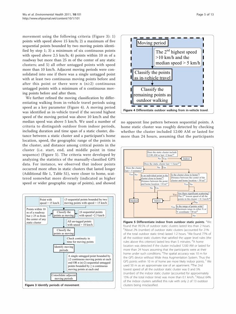
movement using the following criteria (Figure 3): 1)points with speed above 15 km/h; 2) a maximum of fivesequential points bounded by two moving points identi-fied by step 1; 3) a minimum of six continuous pointswith speed above 2.5 km/h; 4) points within 10 m of aroadway but more than 25 m of the center of any staticclusters; and 5) all other untagged points with speedmore than 10 km/h. Adjacent moving periods were con-solidated into one if there was a single untagged pointwith at least two continuous moving points before andafter this point or there were n (n≥2) continuousuntagged points with a minimum of n continuous mov-ing points before and after them.We further refined the moving classification by differ-

entiating walking from in-vehicle travel periods usingspeed as a key parameter (Figure 4). A moving periodwas identified as in-vehicle travel if the second highestspeed of the moving period was above 10 km/h and themedian speed was above 5 km/h. We used a number ofcriteria to distinguish outdoor from indoor periods,including duration and time span of a static cluster, dis-tance between a static cluster and a participant’s homelocation, speed, the geographic range of the points inthe cluster, and distance among critical points in thecluster (i.e. start, end, and middle point in timesequence) (Figure 5). The criteria were developed byanalyzing the statistics of the manually-classified GPSdata. For instance, we observed that indoor pointsoccurred more often in static clusters that lasted longer(Additional file 1, Table S1), were closer to home, scat-tered somewhat more diversely (indicated as higherspeed or wider geographic range of points), and showed

no apparent line pattern between sequential points. Ahome static cluster was roughly detected by checkingwhether the cluster included 12:00 AM or lasted formore than 24 hours, assuming that the participants

Classify the points as moving

5 sequential points bounded by two moving points with speed > 15 km/h

Point with speed > 15 km/h

Points within 10 m of a roadway but 25 m from the center of any static cluster

6 sequential points with speed >2.5 km/h

All un-tagged points with speed > 10 km/h

Identify moving periods

Classify the points as moving

Check continuity in time for moving points

A single untagged point bounded by 2 continuous moving points at each

end OR n (n 2) sequential untagged points bounded by n continuous moving points at each end

Consolidate adjacent moving periods

Figure 3 Identify periods of movement.

Moving period

The 2nd highest speed >10 km/h and the median speed > 5 km/h

Classify the points as in-vehicle travel

Classify the remaining points as

outdoor walking

Figure 4 Differentiate outdoor walking from in-vehicle travel.

YesNoDoes the static cluster last >1 hour?b

Is the cluster close to homed?Distance between the center of the cluster and home location < 50 m?f

Are there significant scattering?The 2nd lowest speed of all the points in the cluster > 0.1 km/h?g

Is the range of points wide?Maximum range in either X or Y coordinate >30 m?h

Does the cluster last < 5 minutes?c

Yes

No

Yes

No

No

Yes

Yes

Outdoor

Is an individual point in the cluster close to homed?Distance between the point and home location <10 m?e

YesNo

No

Indoor

Does the static cluster include 12:00 AM or last >2 hour?a

YesNo Indoor

Figure 5 Differentiate indoor from outdoor static points. aWefound that 99.5% of outdoor static clusters lasted less than 2 hours.bAbout 2% (number) of outdoor static clusters (accounted for 21%of the total outdoor static time) lasted 1-2 hours. cWe found 77% ofall the outdoor static clusters that satisfied the upper level rules (therules above this criterion) lasted less than 5 minutes. dA homelocation was detected if the cluster included 12:00 AM or lasted formore than 24 hours assuming that the participants were at theirhome under such conditions. eThe spatial accuracy was 10 m forthe GPS device without Wide Area Augmentation System. Thus theGPS points within 10 m of home are more likely indoor points. f Weused 50 m as an approximate size of an apartment. gThe 2ndlowest speed of all the outdoor static cluster was 0 and 5%(number) of the indoor static cluster (accounted for approximately15% of the total indoor time) was more than 0.1 km/h. hAbout 64%of the indoor clusters satisfied this rule with only 2 of 13 outdoorclusters being misclassified.


of 13

were at their home under such conditions. We did notattempt to classify other types of locations (e.g. work,school, shopping) because without additional data wehave to make many assumptions on the patterns ofthese activities, which may introduce a lot ofuncertainties.

Random Forest ClassificationAs an alternative to the rule-based algorithm, we applieda machine learning model, random forest [42], to clas-sify the GPS data into different time activity categories.Here, a forest refers to a constellation of many decisiontree models. Because a forest consists of many trees, itis more stable and less prone to prediction errors as aresult of data perturbations [42]. Random forest is con-sidered one of the most accurate general-purpose learn-ing techniques available [43] and has been alreadywidely used in bioinformatics [44,45]. Random forestcreates multiple classification and regression (CART)trees, each trained on a bootstrap sample of the originaltraining data and searches across a randomly selectedsubset of input variables to determine the split. Eachtree in the forest gives or “votes” for a classification (e.g.time activity category). The forest chooses the classifica-tion having the most votes over all the trees in theforest.In this study, we used an R interface in Waikato

Environment for Knowledge Analysis (WEKA) 3.6 soft-ware, a popular machine learning workbench developedby researchers in University of Waikatoi [46,47]. Weexamined the following types of variables: accelerationrate, speed, distance difference, and distance ratio.Acceleration was calculated as the change in speedbetween a given point and the previous sequential point.The distance difference was calculated for any threesequential points as we described above for the rule-based model. The distance ratio was calculated for a ser-ies of sequential points as the ratio between (a) distancebetween the first sequential point and the last sequentialpoint in the series and (b) the sum of the distance forall line segments formed by sequential points in the ser-ies. Speed, distance difference, and distance ratio vari-ables were calculated under various averaging timeintervals ranging from 2 to 60 minutes and centered ateach GPS point. Speed and distance difference wereexpressed as minimum, median, and maximum values.Standard deviation was also calculated for distance dif-ference. Final variables were selected by checking thevariable importance index (a measure of the relativeimportance of the variables) generated from the modeldiagnostics and the correlations among the variables.We first selected 20 most important variables that werenot highly correlated with each other (r < 0.75). Thenwe run the model again with these variables and

selected the most important variables with the p-valueof the z-score < 0.001 for all the variables. Sensitivitytests were conducted for the maximum depth of a treeand the number of trees. Two separate models weredeveloped based on the HCTLS data (hereafter HCTLSrandom forest model) and the supplemental UCI data(hereafter UCI random forest model). For both models,we randomly selected a subset of indoor points (N =30,000 for the HCTLS data and N = 5,000 for the UCIdata) in addition to all outdoor static, outdoor walking,and in-vehicle travel points in the original datasets astraining data.

Model EvaluationTime activity classifications of GPS data based on modelpredictions were compared to those from manually-clas-sified data for both the HCTLS and the supplementaldatasets. There is no “gold-standard” against which tocompare the classification of GPS-derived time activitydata. In this study we used the manually-classified timeactivity classifications as the basis of model evaluationbecause these time activity codes were developed basedon extensive quality assurance checks that involvedcareful inspection of real-time GPS locations in GISusing map overlays, comparison with participant activitylogs, and clarifications from follow-up interviews withparticipants and staff. We examined the sensitivity (theability of the model to identify specific cases), specificity(the ability of the model to identify non-cases), and pre-cision (the proportion of predicted cases that are cor-rectly real cases) of model prediction for each timeactivity category. Both the rule-based and the randomforest models were evaluated against the HCTLS dataand the supplemental UCI data. The two random forestmodels were evaluated using a repeated 10-fold crossvalidation method that has been recommended formodel selection [48,49]. More specifically, the datasetwas randomly split into 10 mutually exclusive subsets ofequal size. The random forest model was trained on 9subsets and validated on the remaining 1 subset of data;the procedure was repeated for 10 times. The reportedvalidation results were the averages from the 10-foldstesting. We further evaluated the capability of the ran-dom forest models in predicting new data by applyingthe HCTLS model to the UCI data and the UCI modelto the HCTLS data.

ResultsWe obtained 406,261 GPS data points from the HCTLSdata after exclusion of points with no time stamp (N =609) and data from one participant who had most ofGPS recordings (N = 16,887) at a one-second interval.Indoor, outdoor static, outdoor walking and in-vehicletravel accounted for 83.4%, 6.1%, 3.3% and 7.2% of the


of 13

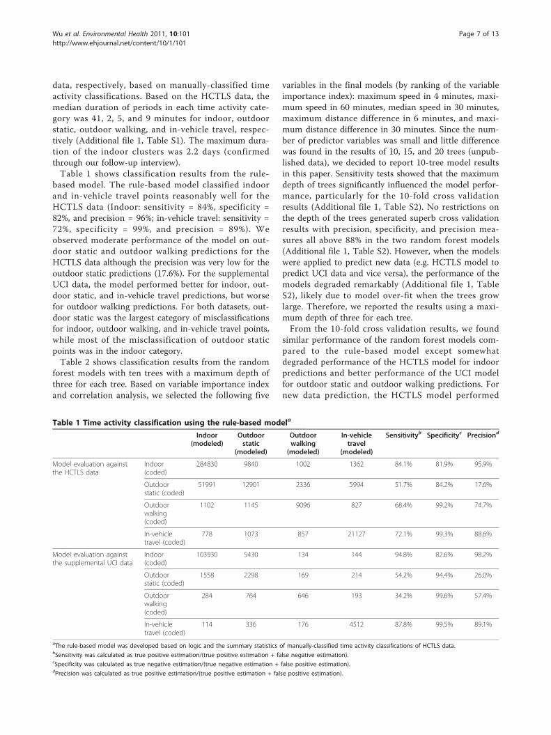
data, respectively, based on manually-classified timeactivity classifications. Based on the HCTLS data, themedian duration of periods in each time activity cate-gory was 41, 2, 5, and 9 minutes for indoor, outdoorstatic, outdoor walking, and in-vehicle travel, respec-tively (Additional file 1, Table S1). The maximum dura-tion of the indoor clusters was 2.2 days (confirmedthrough our follow-up interview).Table 1 shows classification results from the rule-

based model. The rule-based model classified indoorand in-vehicle travel points reasonably well for theHCTLS data (Indoor: sensitivity = 84%, specificity =82%, and precision = 96%; in-vehicle travel: sensitivity =72%, specificity = 99%, and precision = 89%). Weobserved moderate performance of the model on out-door static and outdoor walking predictions for theHCTLS data although the precision was very low for theoutdoor static predictions (17.6%). For the supplementalUCI data, the model performed better for indoor, out-door static, and in-vehicle travel predictions, but worsefor outdoor walking predictions. For both datasets, out-door static was the largest category of misclassificationsfor indoor, outdoor walking, and in-vehicle travel points,while most of the misclassification of outdoor staticpoints was in the indoor category.Table 2 shows classification results from the random

forest models with ten trees with a maximum depth ofthree for each tree. Based on variable importance indexand correlation analysis, we selected the following five

variables in the final models (by ranking of the variableimportance index): maximum speed in 4 minutes, maxi-mum speed in 60 minutes, median speed in 30 minutes,maximum distance difference in 6 minutes, and maxi-mum distance difference in 30 minutes. Since the num-ber of predictor variables was small and little differencewas found in the results of 10, 15, and 20 trees (unpub-lished data), we decided to report 10-tree model resultsin this paper. Sensitivity tests showed that the maximumdepth of trees significantly influenced the model perfor-mance, particularly for the 10-fold cross validationresults (Additional file 1, Table S2). No restrictions onthe depth of the trees generated superb cross validationresults with precision, specificity, and precision mea-sures all above 88% in the two random forest models(Additional file 1, Table S2). However, when the modelswere applied to predict new data (e.g. HCTLS model topredict UCI data and vice versa), the performance of themodels degraded remarkably (Additional file 1, TableS2), likely due to model over-fit when the trees growlarge. Therefore, we reported the results using a maxi-mum depth of three for each tree.From the 10-fold cross validation results, we found

similar performance of the random forest models com-pared to the rule-based model except somewhatdegraded performance of the HCTLS model for indoorpredictions and better performance of the UCI modelfor outdoor static and outdoor walking predictions. Fornew data prediction, the HCTLS model performed

Table 1 Time activity classification using the rule-based modela

Indoor(modeled)

Outdoorstatic

(modeled)

Outdoorwalking

(modeled)

In-vehicletravel

(modeled)

Sensitivityb Specificityc Precisiond

Model evaluation againstthe HCTLS data

Indoor(coded)

284830 9840 1002 1362 84.1% 81.9% 95.9%

Outdoorstatic (coded)

51991 12901 2336 5994 51.7% 84.2% 17.6%

Outdoorwalking(coded)

1102 1145 9096 827 68.4% 99.2% 74.7%

In-vehicletravel (coded)

778 1073 857 21127 72.1% 99.3% 88.6%

Model evaluation againstthe supplemental UCI data

Indoor(coded)

103930 5430 134 144 94.8% 82.6% 98.2%

Outdoorstatic (coded)

1558 2298 169 214 54.2% 94.4% 26.0%


284 764 646 193 34.2% 99.6% 57.4%

In-vehicletravel (coded)

114 336 176 4512 87.8% 99.5% 89.1%

aThe rule-based model was developed based on logic and the summary statistics of manually-classified time activity classifications of HCTLS data.bSensitivity was calculated as true positive estimation/(true positive estimation + false negative estimation).cSpecificity was calculated as true negative estimation/(true negative estimation + false positive estimation).dPrecision was calculated as true positive estimation/(true positive estimation + false positive estimation).


of 13

Table 2 Time activity classification using the random forest modelsa

Indoor(modeled)

Outdoorstatic

(modeled)

Outdoorwalking

(modeled)

In-vehicletravel

(modeled)

Sensitivityb Specificityc Precisiond

HCTLSrandomforest modele

10-fold crossvalidationf

Indoor(coded)

21959 6177 1604 260 73.2% 81.8% 64.1%

Outdoorstatic(coded)

9777 9749 3596 1830 39.1% 81.7% 42.3%


1052 1820 9931 477 74.8% 92.9% 62.5%

In-vehicletravel(coded)

1475 5307 750 21762 74.3% 96.2% 89.4%

Evaluation against thefull UCI dataset

Indoor(coded)

82874 26278 170 314 75.6% 91.6% 98.9%


850 3137 35 214 74.1% 76.2% 10.1%


101 993 555 244 29.3% 99.8% 67.7%


0 515 60 4562 88.8% 99.3% 85.5%

UCI randomforestmodelg

10-fold crossvalidationf

Indoor(coded)

3978 860 120 42 79.6% 99.0% 97.3%


109 3285 471 371 77.5% 90.2% 73.6%


0 170 1313 410 69.4% 94.4% 62.1%


0 146 210 4781 93.1% 92.6% 85.3%

Evaluation against thefull the full HCTLSdataset

Indoor(coded)

153216 54796 128829 1894 45.2% 92.8% 96.9%


3519 6590 13015 1828 26.4% 84.5% 10.0%


320 725 11840 395 89.2% 63.0% 7.5%


999 3464 3550 21281 72.6% 98.9% 83.8%

aThe results reported here came from random forest models with 10 trees and a maximum depth of 3 for each tree.bSensitivity was calculated as true positive estimation/(true positive estimation + false negative estimation).cSpecificity was calculated as true negative estimation/(true negative estimation + false positive estimation).dPrecision was calculated as true positive estimation/(true positive estimation + false positive estimation).eThe model was developed based on all outdoor static, outdoor walking, in-vehicle travel and randomly selected 30,000 indoor pointsfThe reported validation results were the averages from repeated 10-fold cross validation.gThe model was developed based on all outdoor static, outdoor walking, in-vehicle travel and randomly selected 5,000 indoor points from the supplemental UCIdata.


of 13

similarly as the rule-based model in predicting UCI data.However, the UCI model performed worse than therule-based model in predicting HCTLS data, likelybecause of the very small and non-representative train-ing dataset for the development of the UCI model. Simi-lar to the rule-based model, we found that the HCTLSmodel most frequently misclassified indoor, outdoorwalking, and in-vehicle travel to outdoor static whileoutdoor static to indoor category. The misclassificationpattern was different for the UCI model, again likelydue to the small and non-representative training data.

DiscussionWe developed, evaluated, and compared two models toclassify time-location patterns based solely on the pub-licly-available roadway data and raw GPS data (three-dimensional location data and the corresponding timestamps) from participants under free living conditions.To our knowledge, this is one of the first studies thatdeveloped models to systematically classify human timeactivity patterns for travel and non-travel activitiesbased on raw GPS tracking data for use in air pollutionepidemiological studies. Three major strengths of thestudy include the use of extensive manually-classifiedtime-activity data from human participants under freeliving conditions for model development, the compari-son of two models in classifying time activity patterns,and additional model validation using supplemental datawhich were carefully collected and coded. The reason-ably good performance of the models indicates feasibilityof using these models to reliably batch-process GPStracking data from free living human subjects.Air pollution epidemiological studies are increasingly

using GPS to track time activity patterns of human sub-jects. However, few studies have used the GPS-derivedtime activity information extensively in exposure assess-ment and epidemiological analysis; rather, most priorstudies rely on questionnaire-reported time activity pat-terns in the analysis. Lack of reliable methods to mineraw GPS data may be one of the major reasons for thelimited and crude classification of these data. Forinstance, a Canadian study assigned all GPS pointswithin 350 m of a residence as home and 400 m of awork place as work, and did not differentiate indoorfrom outdoor environments [50]; such an approachcould lead to substantial exposure misclassification. Agrowing body of transportation and physical activity lit-erature has begun to provide insights into methods forautomating the classification of GPS to identify differenttravel modes during periods of travel [26-34]. However,since our focus is to develop and evaluate procedures toclassify GPS data for travel and non-travel periods giventhe paucity of applicable methods in the air pollutionepidemiological literature, we do not provide a

comprehensive overview of the transportation and phy-sical activity literature.Overall we found no striking differences in the perfor-

mance of the rule-based model and the random forestmodels. Both models have advantages and disadvan-tages. The rule-based model features high flexibility andeasy-to-interpret results, but the effort involved in themodel development is substantial and may require a lotof additional data and resources. The random forestmodel is easy to use and requires minimum user inter-ference, but it faces a potential over-fitting problem ifnot properly trained and difficulty in results interpreta-tion. In terms of computational time, random forest wasfaster than the rule-based model (e.g. it took approxi-mately one hour for the rule-based model to predict theHCTLS data while < 30 seconds for the random forestto build the model for the same dataset on a 64-bitcomputer with 16 GB of memory and a 2.93 GB Intel®

Core™ i7 Quad Core Processor). However, since ran-dom forest model is purely data driven, it may be moreseverely affected by biased or unrepresentative trainingdata than the rule-based model. In fact, we observedpoor model performance when the UCI random forestmodel was applied to predict the HCTLS data. Withhigh quality training data, random forest model shouldbe a good choice to quickly identify important predictorvariables, develop exploratory models, or even finalmodel based on its performance.For the rule-based model, we observed similar model

performance for indoor and outdoor static predictionsbetween the HCTLS data and the supplemental UCIdata. We observed improved model performance for in-vehicle travel and degraded performance for outdoorwalking predictions in the UCI data. The inferior modelperformance for outdoor walking in the UCI data maybe because over 85% of the limited outdoor walkingdata (a total of approximately 8 hours) came from oneof the staff during his one-day tour to the Sea Worldtheme park in San Diego. It is difficult to distinguishwalking from the other activities since the tour wasassociated with brisk walking, frequent short stops, slowwalking speed, and potentially high uncertainties in thecoding of this type of activity. As expected, most of hiswalking points were misclassified by the rule-basedmodel as outdoor static (Table 1). Even though most ofthe thresholds for classification rules were developedbased on the HCTLS data, we observed better resultsfrom the rule-based model for the other type of time-activity patterns (i.e. indoor, outdoor static, and in-vehi-cle travel) for the supplemental UCI data, indicating theimportance of accurate diary data (in this case moreaccurate indoor and in-vehicle travel coding in the UCIdata) for model development, training, and validation.We did not test whether the performance of the rule-


of 13

based model would be improved if we refined classifica-tion rules using statistics from the UCI data becausethese data were limited to only three subjects who wereindoors 87% of the time and had non-representativeoutdoor walking data. In addition, model performancemay also be influenced by the different GPS devicesused in the two dataset; however, we cannot determinethis impact based on available data. We suggest avoidingthe use of different GPS devices where a single timeactivity model is to be used for all of the GPS data.We found that misclassifying between indoor and out-

door static points was one of the most severe problemsin both the rule-based and the random forest models. InSouthern California, the majority of residential homesare wood structures that do not block satellite signalsappreciably. In addition, for outdoor locations adjacentto buildings structures, GPS signals may be reflected bythe buildings and result in positional error [24]. Becauseof the above reasons, the quality of the GPS data didnot differ much between indoor and outdoor microen-vironments, which makes it difficult to differentiate thetwo under static conditions. Although we included thescatter patterns of the static clusters to differentiateindoor vs. outdoor static conditions (Figure 5), thesemeasures did not do well as shown in our results. Out-door walking and in-vehicle travel were also frequentlymisclassified as outdoor static under low speed condi-tions (e.g., start or end of the trip near a static cluster).For in-vehicle travel, approximately 80% of the pointsthat were wrongly classified as outdoor static pointsoccurred when the participants stayed in the car withoutmoving (e.g., waiting to pick up someone) or the carmoved very slowly approaching or leaving a parking lot(results not shown). The models usually classified vehi-cle idling longer than two minutes or vehicle moving atvery low speed as outdoor static, whereas participantsusually reported such conditions as in-vehicle travel.One the other hand, we found that approximately 75%of the outdoor static points that were wrongly classifiedas in-vehicle travels lasted less than two minutes, indi-cating that this type of misclassification came fromeither coding errors (e.g., participants and research staffmay have difficulty correctly reporting/coding the startor end of an in-vehicle travel period compared to anoutdoor static period) or modeling errors (e.g., the mod-els were incapable of reliably classifying time activitycategories near the start or end of an activity).Three major limitations exist in this study. First, the

manually-classified time activity classifications of theHCTLS and UCI data were not error free despite theextensive measures we have taken to minimize errorsand enhance the accuracy of the coding (e.g., GPS track-ing was combined with a paper diary and in-personinterview). Participants in the HCTLS tended to not

record short stops or trips such as walking to an adja-cent school to pick up a child from school or walking toa nearby corner store [37]. Although follow-up inter-views were used to clarify these discrepancies and tofinalize the classifications of these missing periods, thesedata may not reliably capture the precise time of transi-tions between indoor and outdoor spaces particularlywhen participants lingered near a building entrance dur-ing the transition. Furthermore, even the most compli-ant participants (including our research staff) may havedifficulty correctly documenting the start and end timeof an activity because it takes time and effort to recordsuch information on a time activity log and this couldinterfere with ongoing activities.The second limitation is that we collected data for 47

participants living in southern Los Angeles County andthree staff volunteers living in Irvine, Orange County.Although the participants traveled throughout theregion, , we did not target data collection for residentsof areas with a more challenging built environment forGPS data collection, such as downtown Los Angeleswhere there are many tall and high-density buildingswhich our previous research indicates could result inmore GPS signal loss and positional error [24]. Com-plete loss of satellite signals indoors, however, may notbe a drawback because it can help determine whetherpeople are indoors or outdoors. Future work is neededto refine the models so that they can classify time activ-ity patterns in a wide range of built environments.The third limitation of the study is that our GPS-

based time-activity patterns were not comprehensiveenough for us to explore more refined time-activity pat-terns. For example, we had little GPS data for othermodes of travel (e.g., bus, biking, and train). Future stu-dies should develop more refined classifications basedon a combination of over-sampling of these travelmodes and using related supplemental GIS data (e.g.,trails and bus and train routes). In addition, we did notlook at the impact of different GPS recording intervalson the model performance since the data were very lim-ited for the other time intervals. Only one subject had1-second interval data (sometimes two seconds due torecording fluctuation); the fluctuation in GPS recordingsat other intervals accounted for only about 3.9% of thedata. We believe the rule-based model can be easilyadjusted to accommodate different recording intervals.Future work should consider if the performance of the

models can be further improved by including supple-mental measurement data, GPS diagnostic parameters,and detailed points-of-interest (POI) information. Add-ing data from a physical activity sensor (pedometer oractigraph) may provide improved discrimination acrossthe indoor and outdoor environments. Certain GPSdevices output diagnostic information such as the


of 13

number of satellites used in the determination of loca-tions, the number of satellites in view, and the dilutionof precision which can influence satellite signal qualityand positional accuracy. Our previous work has shownthat horizontal dilution of precision was a good measureof spatial accuracy of the GPS data and may be helpfulin distinguishing indoor vs. outdoor points [24]. Otherstudies have shown the number of satellites used in thelocation determination and the number of satellites inview can be used to improve classifications of GPS data[51]. However, our GPS data did not contain such infor-mation. Commercial POI data provide information onbuilding and facility type (e.g. school, shopping, restau-rant, hospital, and park) and are available from a num-ber of companies (e.g., Garmin) with the mainapplication being in GPS-based tracking and mappingsoftware. Such POI data can help refine models to betterclassify different microenvironments (e.g. residence,school, restaurant) and time activity patterns (e.g. travelmode) and improve exposure assessment of air pollu-tants [27].As we discussed above, this study was limited by input

data quality (e.g. error in manually-classified time activ-ity classifications) and quantity (e.g. lack of GPS diag-nostic and physical activity data). Despite thelimitations, our models showed promising results inidentifying time-location patterns in air pollution healthstudies where exposure levels vary remarkably by loca-tion (e.g. indoor, outdoor, and in-transit). With technol-ogy advances, the data quality and quantity will beimproved significantly in the future research. Forinstance, some GPS devices (e.g. VGPS-900 fromVisiontac™) can voice tag POI, which can improve themanually-classified time activity classifications. In addi-tion, certain physical activity monitors (e.g. GT3X+activity monitor from ActiGraph™) records both activitylevel and ambient light - an intriguing parameter fordistinguishing indoor vs. outdoor environment. In addi-tion to the ease of use and the minimal learning curve,the random forest model is capable of handling a largenumber (hundreds to thousands) of variables, whichmakes it a suitable modeling tool in future studies thatmay collect many types of measurement data in hightemporal resolutions (e.g. GPS, actigraph, and electro-cardiogram data). With appropriate data, the model canbe easily adapted to classify both time-location and phy-sical activity levels, which will advance the understand-ing of potential interactions between air pollutionexposure and physical activity levels on health out-comes. In addition to air pollution epidemiology, themodel can also be applied in other public health fields,such as physical activity and obesity research. Moreeffort is needed to modify and validate the rule-basedmodel before it can incorporate or classify other types

of data. But the rule-based model can be a good choiceif the researchers have a good understanding of the dataand if the decision tree approach cannot capture certainpatterns in the data.

ConclusionsWe successfully developed and evaluated two models toidentify indoor and in-vehicle travel periods from rawGPS data under free living conditions. The rule-basedmodel classified indoor and in-vehicle travel points rea-sonably well, but the performance was moderate foroutdoor static and outdoor walking predictions. Nostriking differences were observed between the rule-based and the random forest models. The random forestmodel was fast and easy to execute, but was likely lessrobust than the rule-based model when the quality ofthe training data was poor.

Additional material

Additional file 1: Supplementary Material, Tables S1 and S2.Statistics of the duration of static clusters and periods of movement ineach time activity category and results of sensitivity tests of maximumdepth in the 10-tree random forest models.

AbbreviationsDOQQ: Digital orthophoto quarter quadrangle; GPS: Global positioningsystem.

AcknowledgementsThe research was supported by the National Institute of EnvironmentalHealth Sciences (NIEHS, R21ES016379 and 3R21ES016379-02S1) and theNational Children’s Study (Formative Research: LOI3-ENV-4-A #14 underContract No. HHSN27555200503415). The HCTLS was supported by theCalifornia Air Resources Board (Contract No. 04-348) and the University ofCalifornia Transportation Center. It would not have been possible withoutthe HCTLS participants who generously allowed us to track their activities formultiple days. We also thank the staff volunteers who provided GPS timeactivity data and are grateful to the valuable insights and assistanceprovided by Lianfa Li, Paul Ong, Arthur Winer, Guillermo Jaimes, WalbertoMartin, Jordan Simms and Carrie Ashendel.

Author details1Program in Public Health, University of California, Irvine, USA. 2Departmentof Epidemiology, School of Medicine, University of California, Irvine, USA.3Department of Planning, Policy and Design, School of Social Ecology,University of California, Irvine, USA. 4Center for Occupational &Environmental Health, University of California, Irvine, USA.

Authors’ ContributionsJW is the PI of this study. JW conceptualized the study, participated in studydesign, method development and data analysis, and drafted the manuscript.CJ conducted the modeling work and data analysis, and helped drafting themanuscript. DH provided the HCTLS GPS time activity dataset, reviewed themanuscript, and revised it critically for important intellectual content. DB andRD helped conceptualize the study and provided important intellectualcontent for the manuscript. All authors assisted in the interpretation ofresults and contributed towards the final version of the manuscript. Allauthors read and approved the final manuscript.

Competing interestsThe authors declare that they have no competing interests.


of 13

http://www.biomedcentral.com/content/supplementary/1476-069X-10-101-S1.DOC

Received: 7 June 2011 Accepted: 14 November 2011Published: 14 November 2011

References1. Brook RD: Is air pollution a cause of cardiovascular disease? Updated

review and controversies. Rev Environ Health 2007, 22:115-137.2. Chen H, Goldberg MS, Villeneuve PJ: A systematic review of the relation

between long-term exposure to ambient air pollution and chronicdiseases. Rev Environ Health 2008, 23:243-297.

3. Englert N: Fine particles and human health–a review of epidemiologicalstudies. Toxicol Lett 2004, 149:235-242.

4. Pelucchi C, Negri E, Gallus S, Boffetta P, Tramacere I, La Vecchia C: Long-term particulate matter exposure and mortality: a review of Europeanepidemiological studies. BMC Public Health 2009, 9:453.

5. Stillerman KP, Mattison DR, Giudice LC, Woodruff TJ: Environmentalexposures and adverse pregnancy outcomes: a review of the science.Reprod Sci 2008, 15:631-650.

6. Chan CC, Ozkaynak H, Spengler JD, Sheldon L: Driver Exposure to VolatileOrganic-Compounds, Co, Ozone, and No2 under Different DrivingConditions. Environmental Science & Technology 1991, 25:964-972.

7. Zhu Y, Eiguren-Fernandez A, Hinds WC, Miguel AH: In-Cabin CommuterExposure to Ultrafine Particles on Los Angeles Freeways. Environ SciTechnol 2007, 41:2138-2145.

8. Westerdahl D, Fruin S, Sax T, Fine PM, Sioutas C: Mobile platformmeasurements of ultrafine particles and associated pollutantconcentrations on freeways and residential streets in Los Angeles.Atmospheric Environment 2005, 39:3597-3610.

9. Briggs DJ, de Hoogh K, Morris C, Gulliver J: Effects of travel mode onexposures to particulate air pollution. Environ Int 2008, 34:12-22.

10. de Nazelle A, Nieuwenhuijsen MJ, Anto JM, Brauer M, Briggs D, Braun-Fahrlander C, Cavill N, Cooper AR, Desqueyroux H, Fruin S, Hoek G, Panis LI,Janssen N, Jerrett M, Joffe M, Andersen ZJ, van Kempen E, Kingham S,Kubesch N, Leyden KM, Marshall JD, Matamala J, Mellios G, Mendez M,Nassif H, Ogilvie D, Peiro R, Perez K, Rabl A, Ragettli M, et al: Improvinghealth through policies that promote active travel: a review of evidenceto support integrated health impact assessment. Environ Int 2011,37:766-777.

11. Weisel CP, Zhang J, Turpin BJ, Morandi MT, Colome S, Stock TH,Spektor DM, Korn L, Winer AM, Kwon J, Meng QY, Zhang L, Harrington R,Liu W, Reff A, Lee JH, Alimokhtari S, Mohan K, Shendell D, Jones J, Farrar L,Maberti S, Fan T: Relationships of Indoor, Outdoor, and Personal Air(RIOPA). Part I. Collection methods and descriptive analyses. Res RepHealth Eff Inst 2005, 1-107, discussion 109-127.

12. Suh HH, Bahadori T, Vallarino J, Spengler JD: Criteria air pollutants andtoxic air pollutants. Environ Health Perspect 2000, 108(Suppl 4):625-633.

13. Wallace L, Nelson W, Ziegenfus R, Pellizzari E, Michael L, Whitmore R,Zelon H, Hartwell T, Perritt R, Westerdahl D: The Los Angeles TEAM study:personal exposures, indoor-outdoor air concentrations, and breathconcentrations of 25 volatile organic compounds. J Expos Anal EnvironEpidemiol 1991, 1:157-192.

14. Klepeis NE, Nelson WC, Ott WR, Robinson JP, Tsang AM, Switzer P, Behar JV,Hern SC, Engelmann WH: The National Human Activity Pattern Survey(NHAPS): a resource for assessing exposure to environmental pollutants.Journal of Exposure Analysis and Environmental Epidemiology 2001,11:231-252.

15. Elgethun K, Yost MG, Fitzpatrick CTE, Nyerges TL, Fenske RA: Comparison ofglobal positioning system (GPS) tracking and parent-report diaries tocharacterize children’s time-location patterns. Journal of Exposure Scienceand Environmental Epidemiology 2007, 17:196-206.

16. Duncan MJ, Mummery WK: GIS or GPS? A comparison of two methodsfor assessing route taken during active transport. American Journal ofPreventive Medicine 2007, 33:51-53.

17. Elgethun K, Fenske RA, Yost MG, Palcisko GJ: Time-location analysis forexposure assessment studies of children using a novel globalpositioning system instrument. Environmental Health Perspectives 2003,111:115-122.

18. Schantz P, Stigell E: A Criterion Method for Measuring Route Distance inPhysically Active Commuting. Medicine and Science in Sports and Exercise2009, 41:472-478.

19. Rainham D, Krewski D, McDowell I, Sawada M, Liekens B: Development ofa wearable global positioning system for place and health research.International Journal of Health Geographics 2008, 7:59.

20. Phillips ML, Hall TA, Esmen NA, Lynch R, Johnson DL: Use of globalpositioning system technology to track subject’s location duringenvironmental exposure sampling. Journal of Exposure Analysis andEnvironmental Epidemiology 2001, 11:207-215.

21. Larsson P, Henriksson-Larsen K: The use of dGPS and simultaneousmetabolic measurements during orienteering. Medicine and Science inSports and Exercise 2001, 33:1919-1924.

22. Stopher P, FitzGerald C, Zhang J: Search for a global positioning systemdevice to measure person travel. Transportation Research Part C-EmergingTechnologies 2008, 16:350-369.

23. Rainham D, McDowell I, Krewski D, Sawada M: Conceptualizing thehealthscape: Contributions of time geography, location technologiesand spatial ecology to place and health research. Social Science &Medicine 2010, 70:668-676.

24. Wu J, Jiang C, Liu Z, Houston D, Jaimes G, McConnell R: Performances ofDifferent Global Positioning System Devices for Time-Location Trackingin Air Pollution Epidemiological Studies. Environ Health Insights 2010,4:93-108.

25. van Dierendock A, Fenton P, Ford T: Theory and Performance of NarrowCorrelator Spacing in a GPS Receiver. Journal of the Institute of Navigation1992, 39:265-283.

26. Chung EH, Shalaby A: A trip reconstruction tool for GPS-based personaltravel surveys. Transportation Planning and Technology 2005, 28:381-401.

27. Bohte W, Maat K: Deriving and validating trip purposes and travel modesfor multi-day GPS-based travel surveys: A large-scale application in theNetherlands. Transportation Research Part C-Emerging Technologies 2009,17:285-297.

28. Du J, Aultman-Hall L: Increasing the accuracy of trip rate informationfrom passive multi-day GPS travel datasets: Automatic trip endidentification issues. Transportation Research Part a-Policy and Practice 2007,41:220-232.

29. Duncan MJ, Mummery WK, Dascombe BJ: Utility of global positioningsystem to measure active transport in urban areas. Medicine and Sciencein Sports and Exercise 2007, 39:1851-1857.

30. Gonzalez PA, Weinstein JS, Barbeau SJ, Labrador MA, Winters PL,Georggi NL, Perez R: Automating mode detection for travel behaviouranalysis by using global positioning systems-enabled mobile phonesand neural networks. Iet Intelligent Transport Systems 2010, 4:37-49.

31. Schuessler N, Axhausen KW: Processing Raw Data from Global PositioningSystems Without Additional Information. Transportation Research Record2009, 28-36.

32. Zheng Y, Liu L, Wang L, Xie X: Learning transportation mode from rawGPS data for geographic applications on the Web. the 11th InternationalConference on World Wide Web; Beijing, China ACM Press; 2008, 247-256.

33. Cooper AR, Page AS, Wheeler BW, Griew P, Davis L, Hillsdon M, Jago R:Mapping the Walk to School Using Accelerometry Combined with aGlobal Positioning System. American Journal of Preventive Medicine 2010,38:178-183.

34. Duncan JS, Badland HM, Schofield G: Combining GPS with heart ratemonitoring to measure physical activity in children: A feasibility study.Journal of Science and Medicine in Sport 2009, 12:583-585.

35. Cho GH, Rodriguez DA, Evenson KR: Identifying Walking Trips Using GPSData. Medicine and Science in Sports and Exercise 2011, 43:365-372.

36. Adams C, Riggs P, Volckens J: Development of a method for personal,spatiotemporal exposure assessment. Journal of Environmental Monitoring2009, 11:1331-1339.

37. Houston D, Ong P, Jaimes G, Winer A: Traffic exposure near the LosAngeles-Long Beach port complex: using GPS-enhanced tracking toassess the implications of unreported travel and locations. Journal ofTransport Geography 2011, 19:1399-1409.

38. Wu J, Funk TH, Lurmann FW, Winer AM: Improving Spatial Accuracy ofRoadway Networks and Geocoded Addresses. Transactions in GIS 2005,9:585-601.

39. Nieuwenhuijsen MJ, Gomez-Perales JE, Colvile RN: Levels of particulate airpollution, its elemental composition, determinants and health effects inmetro systems. Atmospheric Environment 2007, 41:7995-8006.


of 13

http://www.ncbi.nlm.nih.gov/pubmed/17894203?dopt=Abstract



























































40. Nieuwenhuijsen MJ, Kaur S: Determinants of Personal Exposure to PM(2.5), Ultrafine Particle Counts, and CO in a Transport Microenvironment.Environmental Science & Technology 2009, 43:4737-4743.

41. Panis LI, de Geus B, Vandenbulcke G, Willems H, Degraeuwe B, Bleux N,Mishra V, Thomas I, Meeusen R: Exposure to particulate matter in traffic: Acomparison of cyclists and car passengers. Atmospheric Environment 2010,44:2263-2270.

42. Breiman L: Random forests. Machine Learning 2001, 45:5-32.43. Biau G: Analysis of a Random Forests model, Technical report, Université

Paris VI. 2010.44. Cutler A, Stevens JR: Random forests for microarrays. Methods in

Enzymology 2006, 411:422-432.45. Khalilia M, Chakraborty S, Popescu M: Predicting disease risks from highly

imbalanced data using random forest. BMC Med Inform Decis Mak 2011,11:51.

46. Bouckaert RR, Frank E, Hall MA, Holmes G, Pfahringer B, Reutemann P,Witten IH: WEKA-Experiences with a Java Open-Source Project. Journal ofMachine Learning Research 2010, 11:2533-2541.

47. Hall M, Frank E, Holmes G, Pfahringer B, Reutemann P, Witten IH: TheWEKA data mining software: an update. SIGKDD Explorations 2009,11:10-18.

48. Kohavi R: A study of cross-validation and bootstrap for accuracyestimation and model selection. Fourteenth International Joint Conferenceon Artificial Intelligence, IJCAI; Montreal, CA 1995, 1137-1143.

49. Kim JH: Estimating classification error rate: Repeated cross-validation,repeated hold-out and bootstrap. Computational Statistics & Data Analysis2009, 53:3735-3745.

50. Nethery E, Leckie SE, Teschke K, Brauer M: From measures to models: anevaluation of air pollution exposure assessment for epidemiologicalstudies of pregnant women. Occupational and Environmental Medicine2008, 65:579-586.

51. Estrin D: Director, Center for Embedded Networked Sensing, an NSFScience and Technology Center, Headquartered at UCLA. Personalcommunication.

doi:10.1186/1476-069X-10-101Cite this article as: Wu et al.: Automated time activity classificationbased on global positioning system (GPS) tracking data. EnvironmentalHealth 2011 10:101.

Submit your next manuscript to BioMed Centraland take full advantage of:

• Convenient online submission

• Thorough peer review

• No space constraints or color figure charges

• Immediate publication on acceptance

• Inclusion in PubMed, CAS, Scopus and Google Scholar

• Research which is freely available for redistribution

Submit your manuscript at www.biomedcentral.com/submit


of 13











automated time activity classification based on global positioning

Documents