automated observation of multi-agent based simulations: a

HAL Id: hal-00738384https://hal.archives-ouvertes.fr/hal-00738384

Submitted on 4 Oct 2012

HAL is a multi-disciplinary open accessarchive for the deposit and dissemination of sci-entific research documents, whether they are pub-lished or not. The documents may come fromteaching and research institutions in France orabroad, or from public or private research centers.

L’archive ouverte pluridisciplinaire HAL, estdestinée au dépôt et à la diffusion de documentsscientifiques de niveau recherche, publiés ou non,émanant des établissements d’enseignement et derecherche français ou étrangers, des laboratoirespublics ou privés.

Automated observation of multi-agent basedsimulations: a statistical analysis approach

Philippe Caillou, Javier Gil-Quijano, Xiao Zhou

To cite this version:Philippe Caillou, Javier Gil-Quijano, Xiao Zhou. Automated observation of multi-agent based simula-tions: a statistical analysis approach. Studia Informatica Universalis, Hermann, 2013. �hal-00738384�

https://hal.archives-ouvertes.fr/hal-00738384

https://hal.archives-ouvertes.fr

Automated observation of multi-agent basedsimulations

A statistical analysis approach

P. Caillou * , J. Gil-Quijano ** , X. Zhou *

* Laboratoire de Recherche en InformatiqueUniversité Paris Sud – INRIA, Orsay 91405, France

[email protected]** CEA, LIST, Laboratoire Information Modèles et Apprentissage, F-91191

Gif-sur-Yvette, [email protected]

Résumé.Multi-agent based simulations (MABS) have been successfully used to model complex

systems in different areas. Nevertheless a pitfall of MABS is that their complexity increases

with the number of agents and the number of different types of behavior considered in the

model. For average and large systems, it is impossible to validate the trajectories of single

agents in a simulation. The classical validation approaches, where only global indicators are

evaluated, are too simplistic to give enough confidence in the simulation. It is then necessary to

introduce intermediate levels of validation. In this paper we propose the useof data clustering

and automated characterization of clusters in order to build, describe andfollow the evolution

of groups of agents in simulations. These tools provides the modeler with anintermediate point

of view on the evolution of the model. Those tools are flexible enough to allow the modeler to

define the groups level of abstraction (i.e. the distance between the groups level and the agents

level) and the underlying hypotheses of groups formation. We give an online application on a

simple NetLogo library model (Bank Reserves) and an offline log application on a more complex

Economic Market Simulation.

Mots-Clés : Complex systems simulation, multi-agents systems, automated observation,auto-mated characterization, clustering, value-test

Studia Informatica Universalis.

2 Studia Informatica Universalis.

1. Introduction

Multi-agent systems (MAS) are specially well suited to representcomplex phenomena from the description of local agent behaviours.The simulation of complex systems using MAS is a cyclic process :the modeler introduces his/her knowledge into the model, runs simula-tions, discovers bugs, pitfalls or unwanted effects, corrects the modeland eventually his/her knowledge, and the cycle restarts. The cycle isover when it is not possible to further improve the model because oftechnical or knowledge limitations.

Once the agents behaviors are defined, the cyclic modeling processusually focuses on fitting global simulation parameters and/or the ini-tial states of agents in order to reproduce global behaviorsobserved inthe modeled empirical phenomena. The global behaviors are usuallyreproduced and tested with global variables (for example, in the caseof socio-spatial models, variables as populations densityand growingrates, or evacuation time and number of death for panic simulations).Those global variables are evaluated both on simulation andon empi-rical data. The calibration of the simulation is achieved byfinding theright set of values (or values intervals) for the agents and global simu-lation parameters which lead to minimize the difference between tra-jectories of global variables in simulation and in empirical data. Thisoptimization-like approach is implemented by several existing frame-works (for example in GAMA [TDV10], see section 2 for an extendedpresentation of these tools).

Nevertheless, this traditional approach may be too simplistic in orderto characterize the dynamics of complex systems. Indeed, ina complexsystem, different phenomena may simultaneously occur at different le-vels (at the agents and at the global levels, but also at intermediatelevels) and influence each other [GQLH10]. For instance, groups ofagents (flocks of birds, social groups, coalitions, etc.) following simi-lar trajectories of states may appear, evolve and disappear. To describeand evaluate the evolution of that type of groups, the observation ofglobal variables is not enough. Moreover, because of the emergent pro-perties of complex systems, those groups may be unexpected,and theirpresence may even be unnoticed because no global variable orany other

3

adapted observation mechanism is provided in the simulator. The signi-ficance and even the existence of groups may then be hidden by theusually huge amount of information generated in a MAS simulations.

In this paper, we introduce the use of statistical-based tools to assistthe modeler in the discovering, following the evolution anddescribinggroups of agents. After an overview of the state of the art (section 2, insection 3, we present two complementary tools, data clustering used todiscover and build groups and value test used to automatically describethose groups. In section 4, we present an observation model that usesthose tools in order to produce automated analysis of the evolution ofgroups in MAS simulations illustrated on a NetLogo simple model. Wepresent a more complex offline application in section 5 and conclude insection 6.

2. State of the art

Multi-agent based simulations have been used with a large num-ber of economic, geographic or social applications. There are severalavailable development frameworks for simulation, some of them user-friendly with specific coding language, such as NetLogo [LM], and withthe possibility to interface with Java code parts (like GAMA[TDV10]).Others use only generic language (usually java or C#), such asMO-DULECO [Pha] or Repast [NCV06, RLJ06]. However, none of theseplatforms integrate any module for automatic group analysis. Based onthese platforms, some analyzer tools, such as LEIA [GKMP08], SimEx-plorer [LR] and [Cai10] were developed to generate and analyze auto-matically simulations.

LEIA [GKMP08] is a parameter space browser for the IODA simu-lation framework[KMP08]. It allows the user to instantly make a visualcomparison of numerous simulations by seeing all their results in paral-lel. It provides the user with a set of transformation and generation toolsfor model, and a set of tests to browse the simulations space.Scoringrules are applied to help the user in identifying interesting configura-tions (such as cyclic or regular behaviors).


SimExplorer/OpenMole [LR] is a software, which aims at providinga generic environment for programming and executing experimental de-signs on complex models. The goals are multiple : (1) to externalize thedevelopment of the model exploration, in order to make available somegeneric methods and tools which can be applied in most of the cases forany model to explore ; (2) to favor the reuse of available components,and therefore lower the investment for good quality model explorationapplications ; (3) to facilitate a quality insurance approach for modelexploration.

[Cai10] is a tool to automatically generate and run new simulationsuntil the results obtained are statistically valid using a chi-square test.It can generate new simulations and perform statistical tests on the re-sults, with an accuracy that increases gradually as the results are produ-ced. This tool can be applied to any RePast-based simulation.It deducesvariables and parameters used and asks the user to choose theconfigura-tion of interest. New simulations are generated, computed and analyzeduntil all the independence tests between parameters/variables are valid.Finally, the test results and their margins of error are presented to theusers.

The aim of these tools is to study several simulations (the parame-ter space), to compare their result and analyze them. However, none ofthem aim at studying one complex simulation to describe it. To exploreone simulation, the only existing tools are the integrated tools (suchas the NetLogo graphs and logs), which are limited to global or user-defined clusters, and classic data mining on logs. We aim to combine theadvantage of online and agent-oriented analysis of NetLogowith theflexibility and descriptive potential of Data Mining tools.Some workusing data mining tool to identify groups and describe them had beenrealised with specific applications, for exemple in the SimBogota simu-lation ([GQPD07][EHT07]). In these simulations, social groups in Bo-gota city regions where identified by data mining, and the group resultswere perceived by the agent. The goal was however more a multi-scalesimulation than a description of simulation dynamic.

5

3. Analysis tools

In this section, we present the two main tools that we use to auto-matically analyze MAS simulations. To discover the groups of agentswe propose to use data clustering, and then value-test evaluations to des-cribe them. These tools are associated in our analysis model(see section4) in order to automatically describe the evolution of groups and helpthe modeler to understand what happens in complex simulations.

3.1. Finding the groups : clustering

The goal of clustering algorithms is to "find the structure" ofa da-taset. Most of the time, data represent objects or individuals that aredescribed by a given number of variables or characteristics[LPM06].The dataset’s structure is represented as a partition or a hierarchy ofpartitions. Every single object is assigned to a given group(cluster) inthe partition, or to a several groups (clusters) when considering a hierar-chy of partitions. An object is assigned to a given groupg if it is moresimilar (the sense of similar varies with the algorithm) to the objects ing than to objects in other groups. The main hypothesis when clusteringa dataset is that the structure exists and the goal is to make it evident. Si-milarity between objects usually depends on the distance between them(actually between the vector of variables representing them). One of themost used distance (for quantitative variables) is the Euclidean distance.

As the state of an agent is a vector that includes the instantaneousvalues of the set of variables that describes the agent’s behavior, we canconsider the set of states of all the agents in a simulation asa datasetand then to cluster it. In that way, groups of agents whose states simi-larity is maximal can get formed. To conduct the clustering,the "right"algorithm and distance measure have to be chosen. Indeed, differentclustering algorithms can lead to different results as their underlying hy-pothesis and functionning diverge. In our work, it is the responsibility ofthe modeler to choose those parameters. By including in our model theWeka machine learning library1, we provide the modeler with a widelist of clustering algorithms and distances functions. In our experiments

1. http ://weka.wikispaces.com/


we used the X-Means algorithm [PM00], described in the following pa-ragraphs.

One of the most known algorithm of clustering is theK-Meansalgo-rithm [Llo82] whose objective is to find thek prototypes (average cha-racteristic vectors) that represents the best the data. In that algorithmk

initial prototypes are defined (usually by random) and at each iterationevery object is assigned to its nearest prototype. Every prototype is thenupdated to the average vector of the characteristics of the objects thatwere assigned to it. The process is repeated until there is nosignificantchanges of prototypes between two succesive iterations or until a maxi-mum number of iterations is reached. The main pitfall of K-Means isthat the numberk of clusters must be known. As the idea of clusteringis to find the right and unknown structure describing the dataset, thereis no reason to knowk beforehand.

An improvement of K-Means is proposed with the X-Means algo-rithm [PM00]. In that algorithm the "right" numberk of clusters is de-termined by successive K-Means executions. The first execution startswith akmin number of clusters (the minimum number of clusters, a pa-rameter of the model), and at each iteration one of the clusters found inthe previous iterations is divided into two new clusters. The cluster tobe divided is the one whose internal similarity (the similarity betweenthe objects inside the cluster) is the lowest. The process isrepeated untilkmax number of clusters is reached. Thenkmax−kmin+1 partitions areproduced. The chosen partition is the one that maximizes theinternalsimilarity of clusters and maximizes the distance between prototypes.

3.2. Interpreting the groups : Value tests

Value test (VT) [Mor84, LPM06] is an indicator that allows the au-tomated interpretation of clusters. It determines the moresignificantfactors (for continuous variables) and modalities (for categorical va-riables) in a given cluster in comparison with the global dataset. TheVT compares the deviation between the variables/modalities in clustersand the variables/modalities in the overall dataset. The main hypothe-sis in the VT calculation is that the variables follow Gaussian distri-butions. In that condition, for a level of risk of 5% we can consider

7

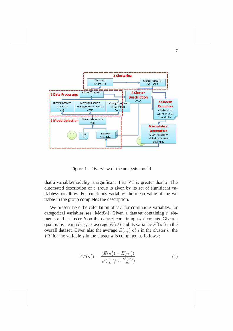
Figure 1 – Overview of the analysis model

that a variable/modality is significant if its VT is greater than 2. Theautomated description of a group is given by its set of significant va-riables/modalities. For continous variables the mean value of the va-riable in the group completes the description.

We present here the calculation ofV T for continuous variables, forcategorical variables see [Mor84]. Given a dataset containing n ele-ments and a clusterk on the dataset containingnk elements. Given aquantitative variablej, its averageE(nj) and its varianceS2(nj) in theoverall dataset. Given also the averageE(nj

k) of j in the clusterk, theV T for the variablej in the clusterk is computed as follows :

V T (njk) =

(E(njk)− E(nj))

√

(n−nk

n−1× S2(nj)

nk)

(1)


4. Analysis model

4.1. Model overview

Our goal is to describe, online or offline, what happens in a simula-tion at the cluster level. Our model can be described with several stepsas illustrated in Fig. 1 :

1) Model Selection : what do we study ?

2) Data processing : what are the data ?

3) Clustering : can we find homogeneous groups ?

4) Cluster description : how can we describe them ?

5) Cluster evolution : how do they evolve ?

6) Simulation generation : is this reproducible ? In future work, weintend to use the most interesting (or user-selected) agentmodel (clus-ters) identified to generate new simulations with similar agents and thustest the clusters behavioral stability.

For a better understanding, we will describe each step with the ap-plication of our tool to an illustrative example.

4.2. Model selection

The first step is to choose the model to be studied. Our model canbeapplied both online (with NetLogo) or offline from logs (by simulatingan online data stream).

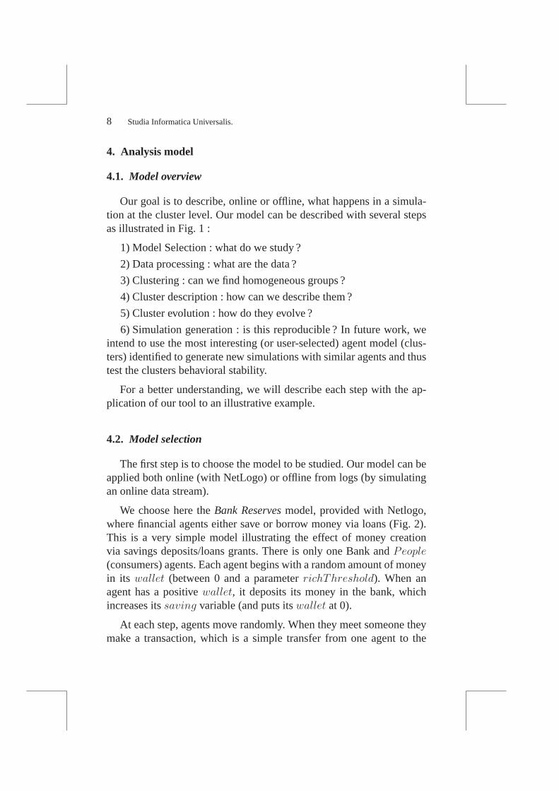
We choose here theBank Reservesmodel, provided with Netlogo,where financial agents either save or borrow money via loans (Fig. 2).This is a very simple model illustrating the effect of money creationvia savings deposits/loans grants. There is only one Bank andPeople

(consumers) agents. Each agent begins with a random amount of moneyin its wallet (between 0 and a parameterrichThreshold). When anagent has a positivewallet, it deposits its money in the bank, whichincreases itssaving variable (and puts itswallet at 0).

At each step, agents move randomly. When they meet someone theymake a transaction, which is a simple transfer from one agentto the

9

Figure 2 – Netlogo Bank Reserves Model

other. When the buyer agent has not enough money (savings orwallet),he takes aloan. The bank grants loans (and creates money) unless thetotal amount ofloans reaches the total amount of deposits (savings)multiplied by a parameter (1-Reserves). In other words, the bank hasto keep aReserve proportion of its deposits which can not be usedfor loans. When an agent receives money (via transactions), it uses itto pay back its loans if it has some. Thewealth of an agent is definedassavings + wallet − loans. For our illustrative experiment, we useReserves = 70, People = 200 andrichThreshold = 20.

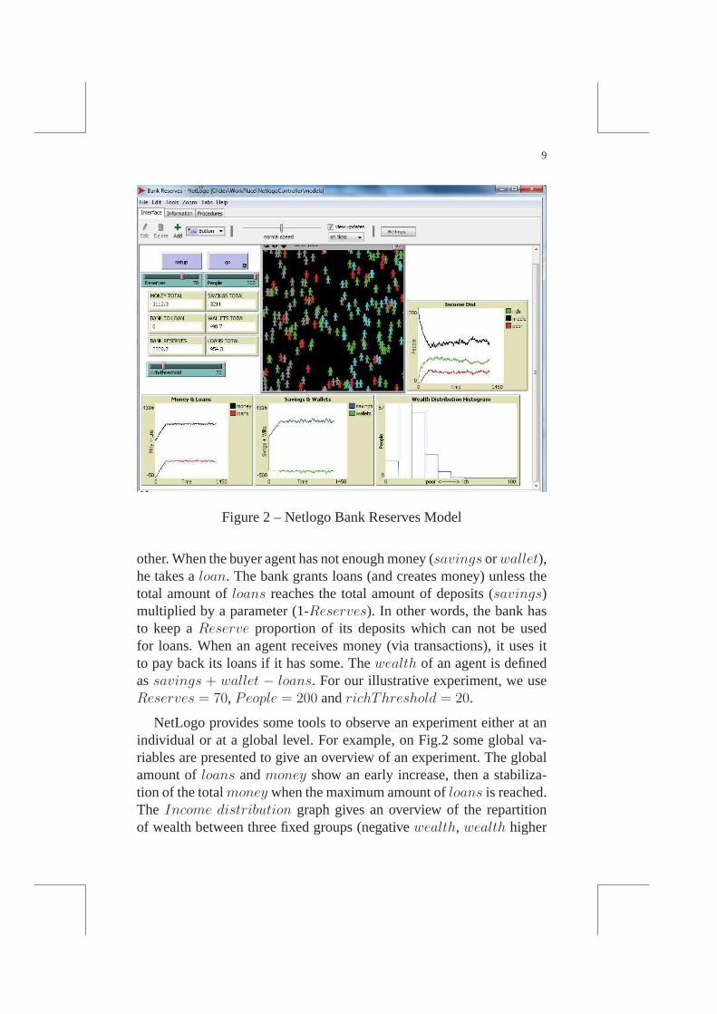
NetLogo provides some tools to observe an experiment eitherat anindividual or at a global level. For example, on Fig.2 some global va-riables are presented to give an overview of an experiment. The globalamount ofloans andmoney show an early increase, then a stabiliza-tion of the totalmoney when the maximum amount ofloans is reached.The Income distribution graph gives an overview of the repartitionof wealth between three fixed groups (negativewealth, wealth higher


Figure 3 – The cluster list panel gives the identity number ofthe agentsincluded in each cluster.

thanrichThreshold and the rest). Even if these informations are inter-esting, a more detailed understanding of the model behaviorcan not bereached with such global/local observation. For example, it is difficultto answer the following questions :who are the wealthy agents ? Do therich stay rich ?This would even be truer for more complex models, forwhich variable interactions are much more difficult to deduce than withsuch a simple toy simulation.

4.3. Data processing

A data matrix is generated everyn steps. A line in the matrix re-presents one agent’s state. Raw data from simulations are notthe onlyinteresting data for cluster’s generation and analysis. Several filters oraggregators can also be used to process the data stream. We usetwodifferent aggregators to complete the initial matrix : i) the moving ave-rage (for each variable, we add a new variable computed as theaverageof the last five steps values) ; ii) the initial values for eachagent (foreach variable, we define a new variable corresponding to the value ofthe variable for this agent at the starting point of the simulation). Theseinitial valuesvariables are not used in the clustering but used latter forthe description of the clusters.

11

4.4. Clustering

Clustering is performed on the final data in order to generate homo-geneous agent groups (for now, X-Means is used, but any othercluste-ring algorithm from Weka can be easily selected instead). Clusters arevisualized in NetLogo (with colors), and their extension and descrip-tion are presented. For example, in Fig. 3, three clusters are identifiedin t=400.

4.5. Cluster’s description

Once the clusters are identified, it is possible to get an easy-to-readdescription by usingV T (see sec. 3.2). The description withV T (Fig.4) makes it easy to interpret and describe them. Positively (respectivelynegatively) significant variables are presented in blue (resp. red) : theiraverage is significantly higher (resp. lower) than the global average.

For example, int = 400, three clusters are identified.Cluster7, with114 agents, is a "poor" cluster, whose agents have lowwealth, savings,wallet and the corresponding moving average variables (MMsavings

andMMwealth), and a higher amount ofloans. Some significant va-riables are (probably) clustering artifacts (Y Cor) or random effects(TOHeading), and will justify our stability analysis.

Similarly, cluster9 regroups the 66”wealthy” people, with highwealth andsavings and fewloans. An interesting result is the signifi-cantT0Wallet variable, corresponding to thewallet value of agents atthe beginning of the simulation. Thewealthy people were significantlyricher than the average at the beginning of the simulation.

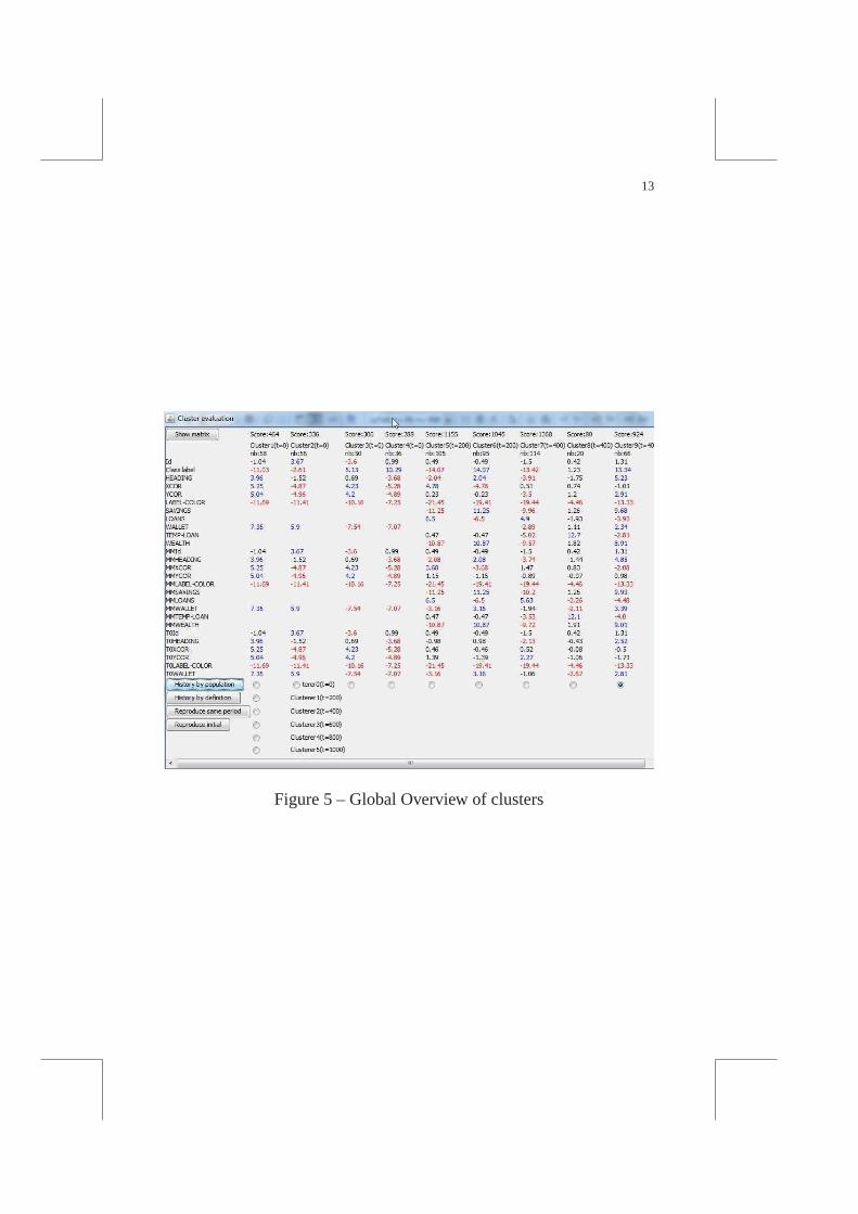
At the end of the simulation, a description of all the clusters obtainedat each time step gives a global overview of the simulation (Fig. 5, witha selection of some results in Table 1). In our experiment, itis alwayspossible to identify awealthy and apoor cluster, and sometimes (like int = 400) amiddle cluster. From their description, it is already possibleto observe that the link between thewealth and the initial wealth (theT0Wallet) is not significant anymore aftert = 400. It may be relatedto the fact (observed with NetLogo global observation) thatbank has


Figure 4 – Cluster Description at t=400 : listed variables arehigher forthe member of the cluster (blue positive value) of lower (rednegativevalues) than in the global population. Black variables are not signifi-cantly different.

13

Figure 5 – Global Overview of clusters


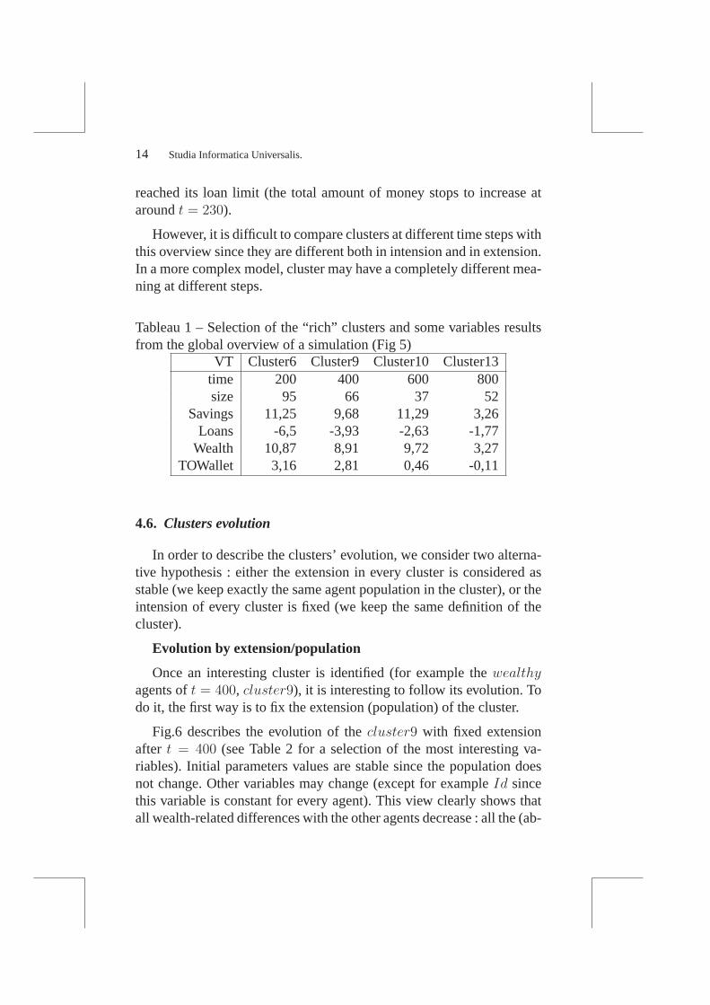
reached its loan limit (the total amount of money stops to increase ataroundt = 230).

However, it is difficult to compare clusters at different time steps withthis overview since they are different both in intension andin extension.In a more complex model, cluster may have a completely different mea-ning at different steps.

Tableau 1 – Selection of the “rich” clusters and some variables resultsfrom the global overview of a simulation (Fig 5)

VT Cluster6 Cluster9 Cluster10 Cluster13time 200 400 600 800size 95 66 37 52

Savings 11,25 9,68 11,29 3,26Loans -6,5 -3,93 -2,63 -1,77

Wealth 10,87 8,91 9,72 3,27TOWallet 3,16 2,81 0,46 -0,11

4.6. Clusters evolution

In order to describe the clusters’ evolution, we consider two alterna-tive hypothesis : either the extension in every cluster is considered asstable (we keep exactly the same agent population in the cluster), or theintension of every cluster is fixed (we keep the same definition of thecluster).

Evolution by extension/population

Once an interesting cluster is identified (for example thewealthy

agents oft = 400, cluster9), it is interesting to follow its evolution. Todo it, the first way is to fix the extension (population) of the cluster.

Fig.6 describes the evolution of thecluster9 with fixed extensionafter t = 400 (see Table 2 for a selection of the most interesting va-riables). Initial parameters values are stable since the population doesnot change. Other variables may change (except for exampleId sincethis variable is constant for every agent). This view clearly shows thatall wealth-related differences with the other agents decrease : all the (ab-

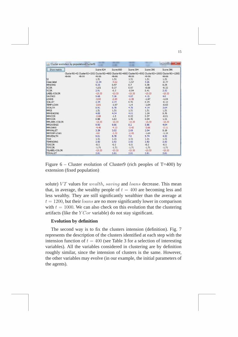
15

Figure 6 – Cluster evolution of Cluster9 (rich peoples of T=400) byextension (fixed population)

solute)V T values forwealth, saving andloans decrease. This meanthat, in average, the wealthy people oft = 400 are becoming less andless wealthy. They are still significantly wealthier than the average att = 1200, but theirloans are no more significantly lower in comparisonwith t = 1000. We can also check on this evolution that the clusteringartifacts (like theY Cor variable) do not stay significant.

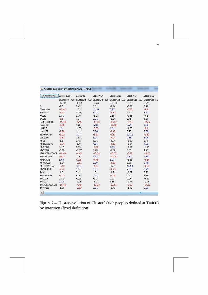
Evolution by definition

The second way is to fix the clusters intension (definition). Fig. 7represents the description of the clusters identified at each step with theintension function oft = 400 (see Table 3 for a selection of interestingvariables). All the variables considered in clustering areby definitionroughly similar, since the intension of clusters is the same. However,the other variables may evolve (in our example, the initial parameters ofthe agents).


Tableau 2 – Evolution of Cluster9 (rich peoples of T=400) by extension :selection of some interesting variables

VT Cluster9 Cluster9 Cluster9 Cluster9 Cluster9time 400 600 800 1000 1200size 66 66 66 66 66

Ycor 2,91 -0,3 -0,04 0,41 2,52Savings 9,68 7,26 4,87 4,15 4

Loans -3,93 -2,85 -2,39 -1,97 -1,04Wealth 8,91 6,78 4,78 4,14 3,64

TOWallet 2,81 2,81 2,81 2,81 2,81

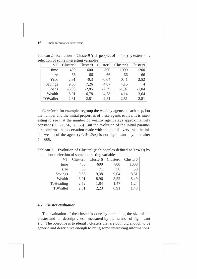
Cluster9, for example, regroup the wealthy agents at each step, butthe number and the initial properties of these agents evolve.It is inter-esting to see that the number of wealthy agent stays approximativelyconstant (66, 71, 56, 58, 65). But the evolution of the initialparame-ters confirms the observation made with the global overview :the ini-tial wealth of the agent (TOWallet) is not significant anymore aftert = 600.

Tableau 3 – Evolution of Cluster9 (rich peoples defined at T=400) bydefinition : selection of some interesting variables

VT Cluster6 Cluster6 Cluster6 Cluster6time 400 600 800 1000size 66 71 56 58

Savings 9,68 9,38 9,04 8,61Wealth 8,91 8,96 8,52 8,49

T0Heading 2,52 1,84 1,47 1,24T0Wallet 2,81 2,23 0,91 1,48

4.7. Cluster evaluation

The evaluation of the cluster is done by combining the size ofthecluster and its ‘descriptivness’ measured by the number of significantV T . The objective is to identify clusters that are both big enough to begeneric and descriptive enough to bring some interesting informations.

17

Figure 7 – Cluster evolution of Cluster9 (rich peoples defined atT=400)by intension (fixed definition)


The score of a clusterc at time stept is calculated as the product ofthe number of significant variables (whose ‘|V T | is greater than 2) :score(c, t) = |V S

c,t| × nc,t whereV Sc,t is the set of significant variables of

c andnc,t is the number of agents inc at the timet.

For example, in Fig. 6, the score of the cluster is initially relativelyhigh (924) because the population is important and the number of si-gnificantV T is high. But since the cluster is not stable (the rich peopledon’t stay rich), the number of significant variables decreases. The scoredecreases, reflecting the fact that the cluster becomes difficult to inter-pret (except by : "the ones that were poor at t=400").

5. Experiments

We tested our analysis tool on several simulation models, both on-line with NetLogo and offline with data logs. Since we have alreadydescribed a NetLogo application in the previous section to illustrate thedescription tool, we will describe here an offline analysis application.

Model description

To illustrate how our model deals with more complex simulations,we chose a model following the KIDS approach [EM04] : the numberof parameters and observed variables is kept high to be more descrip-tive and realistic rather than synthetic. The Rungis Wholesale Marketsimulation [CCB09a][CCB09b] was developed with the BitBang Fran-mework [BMC06] and reproduces a Fruit and Vegetable wholesalemar-ket. One type of seller agent and 4 types of Buyer agents are conside-red in the simulation (with many variable parameters, 20 variables inaverage by agent type). The four type of buyer agents are : Restora-tors seeking efficiency, TimeFree seeking good opportunities, Barbesseeking low-quality and low price products and Neuilly buyers seekinghigh quality high prices products. The csv logs record one line for eachcouple day/agent, with 33 output variables (see below). We analyze hereonly the 60 Buyer agents during the first 10 days of the simulation.

The main observed variables of this model are the transaction time,the number of sellers per buyer, the quality and quantity of the productsand the prices. There are four types of prices, the producer price (price

19

paid by the sellers to the producers), the transaction price(price paid bythe buyers to the sellers), the standard price (price given at the beginningof the transaction) and the final price (price paid by the consumers).In generalproducerprice < transactionprice < standardprice <

finalprice.

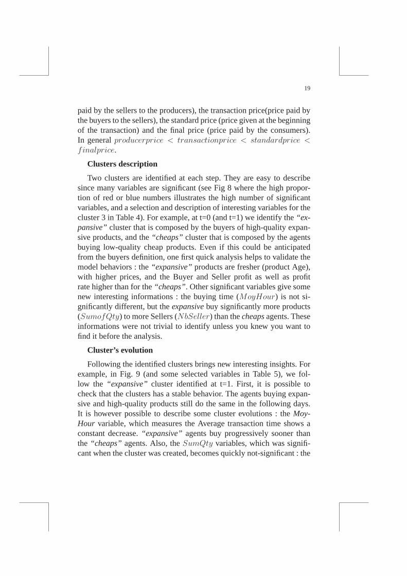
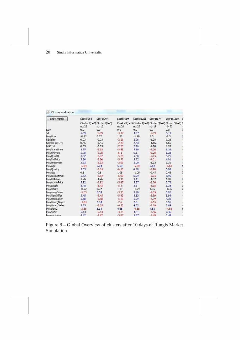
Clusters description

Two clusters are identified at each step. They are easy to describesince many variables are significant (see Fig 8 where the highpropor-tion of red or blue numbers illustrates the high number of significantvariables, and a selection and description of interesting variables for thecluster 3 in Table 4). For example, at t=0 (and t=1) we identify the“ex-pansive”cluster that is composed by the buyers of high-quality expan-sive products, and the“cheaps” cluster that is composed by the agentsbuying low-quality cheap products. Even if this could be anticipatedfrom the buyers definition, one first quick analysis helps to validate themodel behaviors : the“expansive” products are fresher (product Age),with higher prices, and the Buyer and Seller profit as well as profitrate higher than for the“cheaps”. Other significant variables give somenew interesting informations : the buying time (MoyHour) is not si-gnificantly different, but theexpansivebuy significantly more products(SumofQty) to more Sellers (NbSeller) than thecheapsagents. Theseinformations were not trivial to identify unless you knew you want tofind it before the analysis.

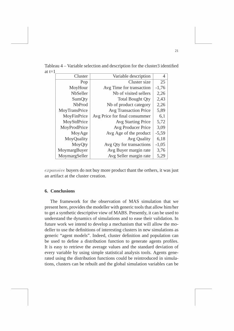
Cluster’s evolution

Following the identified clusters brings new interesting insights. Forexample, in Fig. 9 (and some selected variables in Table 5), we fol-low the “expansive” cluster identified at t=1. First, it is possible tocheck that the clusters has a stable behavior. The agents buying expan-sive and high-quality products still do the same in the following days.It is however possible to describe some cluster evolutions :the Moy-Hour variable, which measures the Average transaction time shows aconstant decrease.“expansive” agents buy progressively sooner thanthe “cheaps” agents. Also, theSumQty variables, which was signifi-cant when the cluster was created, becomes quickly not-significant : the


Figure 8 – Global Overview of clusters after 10 days of Rungis MarketSimulation

21

Tableau 4 – Variable selection and description for the cluster3 identifiedat t=1

Cluster Variable description 4Pop Cluster size 25

MoyHour Avg Time for transaction -1,76NbSeller Nb of visited sellers 2,26SumQty Total Bought Qty 2,43NbProd Nb of product category 2,26

MoyTransPrice Avg Transaction Price 5,89MoyFinPrice Avg Price for final consummer 6,1MoyStdPrice Avg Starting Price 5,72

MoyProdPrice Avg Producer Price 3,09MoyAge Avg Age of the product -5,59

MoyQuality Avg Quality 6,18MoyQty Avg Qty for transactions -1,05

MoymargBuyer Avg Buyer margin rate 3,76MoymargSeller Avg Seller margin rate 5,29

expansive buyers do not buy more product thant the orthers, it was justan artifact at the cluster creation.

6. Conclusions

The framework for the observation of MAS simulation that wepresent here, provides the modeller with generic tools thatallow him/herto get a synthetic descriptive view of MABS. Presently, it canbe used tounderstand the dynamics of simulations and to ease their validation. Infuture work we intend to develop a mechanism that will allow the mo-deller to use the definitions of interesting clusters in new simulations asgeneric “agent models”. Indeed, cluster definition and population canbe used to define a distribution function to generate agents profiles.It is easy to retrieve the average values and the standard deviation ofevery variable by using simple statistical analysis tools.Agents gene-rated using the distribution functions could be reintroduced in simula-tions, clusters can be rebuilt and the global simulation variables can be


Tableau 5 – Evolution by extension of theexpansive group detected att=1 (cluster3)

Day 1 2 3 4 5 6Pop 25 25 25 25 25 25

MayHour -1,76 -2,22 -3,37 -3,21 -2,85 -3,61NbSeller 2,26 1,3 0,77 0,63 1,99 -1,12SumQty 2,43 1,82 0,83 1,3 3,53 -0,53NbProd 2,26 1,3 0,77 0,63 1,99 -1,12

MoyTransPrice 5,89 4,52 5,14 5,09 5,84 4,42MoyFinPrice 6,1 5,36 5,38 5,67 6,25 5,5MoyStdPrice 5,72 3,42 2,87 3,28 4,84 2,8

MoyProdPrice 3,09 0,88 2,32 2,94 3,48 1,96MoyAge -5,59 -4,73 -4,77 -5,34 -5,57 -4,91

MoyQuality 6,18 4,96 5,23 5,59 6,16 5,14MoyQty -1,05 0,63 -0,13 1,03 1,79 1,33

MoymargBuyer 3,76 5 4,14 4,91 4,76 4,77MoymargSeller 5,29 3,95 4,45 3,97 4,83 3,95

Figure 9 – Evolution by extension of theexpansive group detected att=1 (cluster3)

23

compared with their previous values. In that way, the clusters stabilityand their "expressiveness" can be measured over different simulations.

In order to allow the analysis of a wide number of different type ofsimulations we are currently adapting our framework both toconsiderqualitative and network variables and facilitate large simulations analy-sis. The latter will be done by integrating our framework to the Open-Mole engine. That engine provides, among other facilities,the easy useof cluster and grid computing for simulations.

Références

[BMC06] T. Baptista, T. Menezes, and E. Costa. Bitbang : A modeland framework for complexity research. InECCS 2006,2006.

[Cai10] Philippe Caillou. Automated multi-agent simulationgene-ration and validation. InPRIMA 2010, page 16p. LNCS,2010.

[CCB09a] Philippe Caillou, Corentin Curchod, and Tiago Baptista.Simulation of the rungis wholesale market : Lessons on thecalibration, validation and usage of a cognitive agent-basedsimulation. InIAT, pages 70–73, 2009.

[CCB09b] Corentin Curchod, Philippe Caillou, and Tiago Baptista.Which Buyer-Supplier Strategies on Uncertain Markets ?A Multi-Agents Simulation. InStrategic Managemtn So-ciety, Washington États-Unis d’Amérique, 2009.

[EHT07] Bruce Edmonds, Cesareo Hernandez, and Klaus Troitzsch,editors. Social Simulation : Technologies, Advances andNew Discoveries, volume 1. Idea Group Inc., 2007.

[EM04] Bruce Edmonds and Scott Moss. From kiss to kids -an ’anti-simplistic’ modelling approach. InMABS, pages130–144, 2004.


[GKMP08] Francois Gaillard, Yoann Kubera, Philippe Mathieu, andSebastien Picault. A reverse engineering form for multiagent systems. InESAW 2008, pages 137–153, 2008.

[GQLH10] Javier Gil-Quijano, Thomas Louail, and GuillaumeHutz-ler. From biological to urban cells : lessons from threemultilevel agent-based models. InPRACSYS 2010 – FirstPacific Rim workshop on Agent-based modeling and simu-lation of Complex Systems, Kolkota, India, 2010. LNCS.

[GQPD07] J. Gil-Quijano, M. Piron, and A. Drogoul. Mechanismsof automated formation and evolution of social-groups :A multi-agent system to model the intra-urban mobilitiesof Bogotá city. InSocial Simulation : Technologies, Ad-vances and New Discoveries, chapter 12, pages 151–168.Idea Group Inc., 2007.

[KMP08] Yoann Kubera, Philippe Mathieu, and S ?bastien Picault.Interaction-oriented agent simulations : From theory to im-plementation. In Malik Ghallab, Constantine Spyropoulos,Nikos Fakotakis, and Nikos Avouris, editors,Proceedingsof the 18th European Conference on Artificial Intelligence(ECAI’08), pages 383–387. IOS Press, 2008.

[Llo82] Stuart P. Lloyd. Least squares quantization in pcm.In IEEETransactions on Information Theory, volume 28, pages129–137, 1982.

[LM] Center For Connected Learning and Computer-Based Mo-deling. Netlogo : http ://ccl.northwestern.edu/netlogo/.

[LPM06] Ludovic Lebart, Marie Piron, and Alain Morineau.Statis-tique exploratoire multidimeensionnelle : visualisationetinférence en fouilles de données. Fourth edition, Dunod,Paris, 2006.

[LR] Mathieu Leclaire and Romain Reuillon. Simexplorer :http ://www.simexplorer.org/.

25

[Mor84] Alain Morineau. Note sur la caractérisation statistiqued’une classe et les valeurs-tests. InBull. Techn. du Centrede Statistique et d’Informatique Appliquées, volume 2,pages 20–27, 1984.

[NCV06] Michael J. North, Nicholson T. Collier, and Jerry R. Vos.Experiences creating three implementations of the repastagent modeling toolkit. InACM Transactions on Modelingand Computer Simulation, volume 16, pages 1–5, 2006.

[Pha] Denis Phan. From agent-based computational economicstowards cognitive economics. InCognitive Economics,Handbook of Computational Economics.

[PM00] Dan Pelleg and Andrew Moore. Xmeans : Extending k-means with efficient estimation of the number of clusters.In 17th International Conference on Machine Learning,pages 727–734, 2000.

[RLJ06] Steven F. Railsback, Steven L. Lytinen, and Stephen K.Jackson. Agent-based simulation platforms : Review anddevelopment recommendations. InSimulation, volume 82,pages 609–623, 2006.

[TDV10] Patrick Taillandier, Alexis Drogoul, and Duc-An Vo.Gama : a simulation platform that integrates geographi-cal information data, agent-based modeling and multi-scalecontrol. InPRIMA 2010, 2010.

automated observation of multi-agent based simulations: a

Documents