Automated Learning of Subcellular Location

Patterns in Confocal Fluorescence Images from

Human Protein Atlas

Jieyue Li

Center for Bioimage informatics,

Department of Biomedical Engineering,

Carnegie Mellon University

jieyuel@andrew.cmu.edu

This a written report of Data Analysis Project (DAP)in lieu of a Masters Thesis at Machine Learning Department

Committee Members:

Dr. Robert F. Murphy

Dr. William W. Cohen

Dr. Jelena Kovacevic

October 19, 2012

1

Abstract

Consecutive to the human genome project, the human proteome project seeks toexplore the function, structure, variability and interaction of proteins which supportthe daily operation of our human bodies. The identification of protein locationswithin cells is an essential part. The appearance of the residence of proteins mayillustrate the status and functioning of cells, and then organs, tissues or systems.Microscopy images have been widely used in this field. However, due to the mas-sive scale of the combinations of proteins and organelles in cell, we are not ableto annotate all images manually. Therefore, we would like to take advantage ofautomated analysis and machine learning skills to build accessible tools to help biol-ogists annotate protein patterns faster and more accurate, and to correct the humanannotations as well.

This project includes two tasks. In the first task, we describe automated ap-proaches to analyze the confocal immunofluorescence images from the Human Pro-tein Atlas (HPA) which show subcellular location for thousands of proteins and arecurrently annotated by visual inspection, and approaches to improve annotation.We began by training Support Vector Machine (SVM) classifiers to recognize theannotated patterns. By ranking proteins according to the confidence of the classifier,we generated a list of proteins that were strong candidates for reexamination. Inparallel, we applied hierarchical clustering to group proteins and identified proteinswhose annotations were inconsistent with the remainder of the proteins in their clus-ter. These proteins were reexamined by the original annotators, and a significantfraction had their annotations changed. The results demonstrate that automatedapproaches can provide an important complement to visual annotation.

In the second task, we address this classification problem using region-based (orpatch-based) computer vision methods. The HPA images contain stains for threereference components and the protein subcellular pattern can be viewed as spatial co-localization between the reference components and the protein distribution. Howeverthere are many other components that are invisible. We first randomly selectedlocal image regions within the cells, and then extracted various carefully designedfeatures from these regions. This region based approach enables us to explicitlystudy the relationship between proteins and different cell components, as well as theinteractions between these components. To achieve these two goals, we propose twodiscriminative models that extend logistic regression with structured latent variables.The first model allows the same protein pattern class to be expressed differentlyaccording to the underlying components in different regions. The second modelfurther captures the spatial dependencies between the components within the samecell so that we can better infer these components. To learn these models, we proposeda fast approximate algorithm for inference, and then used gradient based methodsto maximize the data likelihood. In the experiments, we show that the proposedmodels help improve the classification accuracies on synthetic data and real cellularHPA images. The best overall accuracy we report in this project is about 84.6% forHPA images, which to our knowledge is the best so far. In addition, the dependencieslearned are consistent with prior knowledge of cell organization.

2

1 Introduction

Knowledge of the subcellular locations of proteins provides critical context necessary for under-standing their functions within the cell. Hence the field of location proteomics is concerned withcapturing informative and defining characteristics of subcellular patterns on a proteome-widebasis [11,14]. Automated methods for systematic study of protein locations, which combine fluo-rescence microscopy techniques with computer vision, pattern recognition and machine learningalgorithms, have been extensively described [11, 6, 16, 23, 21]. Most of these studies involve ex-tracting subcellular location features (SLFs) from images or cells [23, 15]. Automated analysisof subcellular patterns has been described for a proteome-scale image collection for yeast [10]and for a wide range of human tissues [24].

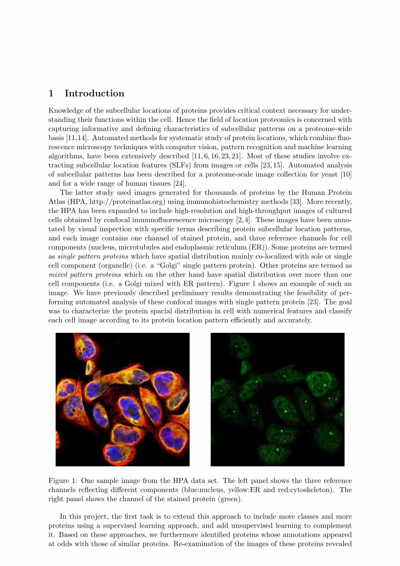
The latter study used images generated for thousands of proteins by the Human ProteinAtlas (HPA, http://proteinatlas.org) using immunohistochemistry methods [33]. More recently,the HPA has been expanded to include high-resolution and high-throughput images of culturedcells obtained by confocal immunofluorescence microscopy [2,4]. These images have been anno-tated by visual inspection with specific terms describing protein subcellular location patterns,and each image contains one channel of stained protein, and three reference channels for cellcomponents (nucleus, microtubules and endoplasmic reticulum (ER)). Some proteins are termedas single pattern proteins which have spatial distribution mainly co-localized with sole or singlecell component (organelle) (i.e. a “Golgi” single pattern protein). Other proteins are termed asmixed pattern proteins which on the other hand have spatial distribution over more than onecell components (i.e. a Golgi mixed with ER pattern). Figure 1 shows an example of such animage. We have previously described preliminary results demonstrating the feasibility of per-forming automated analysis of these confocal images with single pattern protein [23]. The goalwas to characterize the protein spacial distribution in cell with numerical features and classifyeach cell image according to its protein location pattern efficiently and accurately.

Figure 1: One sample image from the HPA data set. The left panel shows the three referencechannels reflecting different components (blue:nucleus, yellow:ER and red:cytoskeleton). Theright panel shows the channel of the stained protein (green).

In this project, the first task is to extend this approach to include more classes and moreproteins using a supervised learning approach, and add unsupervised learning to complementit. Based on these approaches, we furthermore identified proteins whose annotations appearedat odds with those of similar proteins. Re-examination of the images of these proteins revealed

3

that a considerable number had been incorrectly annotated. Thus, our approaches can be usednot only for the purpose of annotations de novo, but also for improving the accuracy of humanannotations. This task has be done in Chapter 2.

We applied feature calculation and multi-class classification methods on the whole cell inthe first task. In order to improve the classification performance, in the second task, we usedregion-based computer vision methods to incorporate more local information about the proteinlocation patterns. As a matter of fact, such a pattern can be represented as the spatial co-localization between protein distribution and various cell components (organelles). However,a key difficulty is that we can only observe three types of reference components due to thelimitation of staining and imaging techniques. Therefore, it is hard to infer the locations of theinvisible components given the observations. For example, we may want to classify a proteininto the class of “Golgi complex” if it mainly overlaps with the Golgi complex, but the Golgicomplex is not directly visible to us in the images. Thereby it is important to uncover theseinvisible parts and then use them for classification from their co-occurrence information withthe protein.

Although invisible, we still have some clues about the presence of a component in someregion of one cell. For instance, one component may have an effect on the appearance of anotheroverlapping and/or interacting component. We can also make inference about the componentin the given image region based on the distribution of certain proteins in the cell (e.g. locationsand shapes), and its relative distances to other components. If we can discover the dependenciesbetween the observed features extracted from regions and the underlying components, as wellas the co-localization relationships between components, then the presence of those hiddencomponents can be inferred and our classification task would be easier. The second task, onthe basis of this intuition, has be done in Chapter 3.

4

2 Automated Analysis and Reannotation of Subcellular Loca-tions in Confocal Images from the Human Protein Atlas

1

2.1 INTRODUCTION

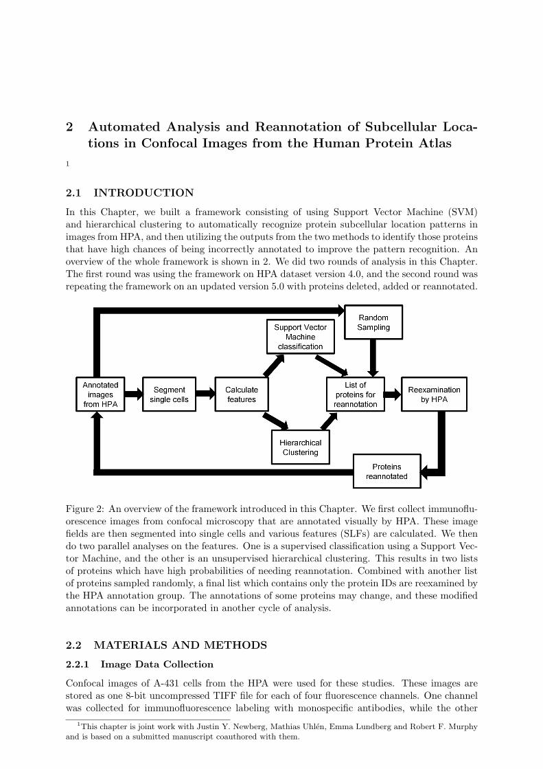
In this Chapter, we built a framework consisting of using Support Vector Machine (SVM)and hierarchical clustering to automatically recognize protein subcellular location patterns inimages from HPA, and then utilizing the outputs from the two methods to identify those proteinsthat have high chances of being incorrectly annotated to improve the pattern recognition. Anoverview of the whole framework is shown in 2. We did two rounds of analysis in this Chapter.The first round was using the framework on HPA dataset version 4.0, and the second round wasrepeating the framework on an updated version 5.0 with proteins deleted, added or reannotated.

Figure 2: An overview of the framework introduced in this Chapter. We first collect immunoflu-orescence images from confocal microscopy that are annotated visually by HPA. These imagefields are then segmented into single cells and various features (SLFs) are calculated. We thendo two parallel analyses on the features. One is a supervised classification using a Support Vec-tor Machine, and the other is an unsupervised hierarchical clustering. This results in two listsof proteins which have high probabilities of needing reannotation. Combined with another listof proteins sampled randomly, a final list which contains only the protein IDs are reexamined bythe HPA annotation group. The annotations of some proteins may change, and these modifiedannotations can be incorporated in another cycle of analysis.

2.2 MATERIALS AND METHODS

2.2.1 Image Data Collection

Confocal images of A-431 cells from the HPA were used for these studies. These images arestored as one 8-bit uncompressed TIFF file for each of four fluorescence channels. One channelwas collected for immunofluorescence labeling with monospecific antibodies, while the other

1This chapter is joint work with Justin Y. Newberg, Mathias Uhlen, Emma Lundberg and Robert F. Murphyand is based on a submitted manuscript coauthored with them.

5

channels were acquired using standard stains for the nucleus, endoplasmic reticulum and mi-crotubule cytoskeleton [2]. After images were acquired, they were visually annotated. One ormore location labels were assigned to each protein (i.e., a protein could be annotated as Golgipattern if it mainly distributes in the Golgi apparatus, or viewed as consisting of a centrosomepattern mixed with cytoplasm pattern). Up to two image fields were taken for each protein.

2.2.2 Cell Segmentation and Feature Calculation

We used the same cell segmentation and feature calculation strategies as in our previous work[23]. The result was a total of 714 features for each cell, for an average of 9 cells per image.The much larger number of features compared to cells in each class suggested the need for somefeature reduction or selection method, and we chose Stepwise Discriminant Analysis as it hasworked well in this field of application [17]. After selection there were around 100 features left.

2.2.3 Support Vector Machine Classification

We trained SVM to classify cells by their subcellular location patterns in two rounds. We uti-lized two levels of nested 5-fold cross-validation so that training parameters could be optimizedwithout using the final testing data. The fraction of representatives of each class within eachfold was kept as close to the original fractions as possible, and all cells for a given protein wereincluded in the same fold to give the most conservative estimate of classification performance.The inner level of cross validation involved using 3 folds for training and one fold for select-ing the optimal values of the radial basis function (RBF) kernel parameter g and the slackparameter C; the outer level used the remaining fold to get the final generalization accura-cies. Additionally, class weights were used during training in order to account for the differentnumber of cells in representing each class. Classification was implemented using the LIBSVMtoolbox [9] (http://www.csie.ntu.edu.tw/ cjlin/libsvm) with one-against-one multi-class SVM(unless otherwise indicated). Since the classifiers output probabilities that each cell belongs tothe classes, we boosted the classification accuracy of single cells by summing class probabilitiesfor all cells for the same protein, and then assigning all of these cells the class with the maximumvalue. For identifying potential proteins that may need to be reannotated, we designed an al-gorithm on the basis of the output probabilities estimated by SVM classifiers. From the outputprobabilities, we find a set of samples (we call set R) that are incorrectly classified but havelow predicted probabilites. These samples are near to the decision boundaries. On the otherhand, there is another set of samples (set F) that are also incorrectly classified but with higherpredicted probabilities, which are farther away from decision boundaries. The fundamental ideaof the algorithm is that R has little impact on F. Even if we flip the labels of samples in R fromtheir previous class labels to the classified labels and train the classifiers again, at least a subsetof samples in F will still be stable and stay in the status of incorrectly classified. ThereforeF are identified as potentially being incorrectly annotated. This algorithm is nonparametricand robust, and bears an analogy to the distillation process. The detailed procedure follows:(1) find the proteins whose automated and human classes disagree and sort them in ascendingorder of classifier-assigned probability; (2) change the annotations for the top N (we used N=5)proteins in this ranked list to match the automated assignment (so that all combinations ofchanges of these labels are considered), and (3) retrain the classifiers and repeat steps 1 and2 for M (we used M=20) levels of recursion. At the end of this process, the proteins thatappeared in all ranked lists were considered for reannotation. In addition to using the classifierfor reannotation, we sought to determine how well it could be used for initial annotation ofproteins. In this case, we do not know a priori which proteins show single patterns and whichshow mixed ones. We applied the classifier (trained on only the single pattern proteins) toimages for 2749 proteins after the second round of reannotation with single or mixed patternswhich have at least 5 proteins, and sorted the proteins by the magnitude of the maximum out-

6

put probability value for each protein. An increasing threshold on this probability was used togenerate precision-recall curves using two approaches for defining precision and recall. In thefirst case of variation, we defined correct classifications as assigning at least one of a protein’slabels correctly with probability above the threshold. In the second case, we defined only as-signments (with probability above the threshold) to single class proteins as correct (and thusall assignments above the threshold made to proteins with two or more labels were consideredincorrect). In our preliminary work on classification of subcellular location patterns using HPAimages [23], a subset of images of single pattern proteins were evaluated by both SVM andRandom Forest [32] methods. The results indicated slightly better performance for the latterapproach, and we therefore also evaluated Random Forest classifiers for the tasks on the largerdatasets used in this project. Since the performance was lower than for SVM (data now shown), we used SVMs throughout this Chapter.

2.2.4 Hierarchical Clustering for Reannotation

As an alternative to classification (which requires labels for training), we used an unsupervisedmachine learning method, hierarchical clustering, to identify candidate proteins for reannota-tion in two rounds. For this we used the same features and a normalized Euclidean distancemetric with Stepwise Discriminant Analysis feature selection. Since there was more than onecell for each protein (and some of these might be atypical), we chose the cell closest to the mul-tivariate median normalized feature value for a given protein to represent that protein in theclustering. The resulting tree can be cut at various values of the distance measure to give dif-ferent numbers of clusters. We defined the cluster annotation for each protein as the dominanthuman annotation in the cluster in which the protein is found. To choose the optimal numberof clusters, Akaike information criterion was used. It balances the log-likelihood of the datagiven the clustering against the number of clusters. After we decided the clustering of proteins,the clusters were ordered by optimal leaf ordering [1] using the associated annotations. Oncewe obtained the clustering of proteins, we computed two scores for each protein to measureand identify the proteins whose annotations might be not correct. The first score is the ratioof the number of proteins of that protein’s class in its cluster to the number of proteins in thedominant (plurality) class of that cluster; the smaller the ratio is, the higher confidence the pro-tein is wrongly annotated. The second score is the normalized feature distance of each proteinto the ”median feature vector” of proteins in that protein’s cluster which have the dominantannotation; a small distance means that the protein is likely to be correctly clustered. In thefirst round, we found a subset of all proteins with the below one value of the first score (in total285 lowest scores by the first definition) and another subset of proteins with the 300 lowestscores by the second definition (which were from the range between zero and the value aroundthe peak of the histogram of the second score, data not shown), and then selected proteins inthe intersection of the two subsets as candidates for reannotation. However, we restricted thefinal list by requiring that each cluster could only have one protein in this list to minimize theeffect that the presence of more than one mis-annotated protein might have on the quality of acluster. In the second round, we released these restrictions. Proteins were sorted with the firstscore and with the second score respectively in ascending order; then they were sorted with thesum of the two ranks ascendingly. As a result, we had all proteins sorted in one list, and themore confidence we had on one protein for its being incorrectly annotated, the higher it wouldbe in the sorting. The final subset of proteins that would be reexamined by annotators wasthus generated from the top until we thought that the number of proteins in the subset wouldnot be an inappropriate burden of work for the annotators.

7

2.2.5 Random Sampling for Reannotation

To serve as a baseline for evaluating the reannotation enrichments we would obtain from au-tomated methods (SVM and hierarchical clustering), we created another list of proteins to bereexamined. Due to the highly imbalanced dataset, we made a compromise schema for the ran-dom sampling. For each class, we uniformly randomly sampled a small number (r) of proteinswith replacement. Thus we were easily able to ensure that we sampled proteins from all classesespecially those with small size and meanwhile to control the number of proteins in this list toreduce the burden of reannotation work. On the other hand, we could reduce the chances ofselecting the majority (or even all) proteins from some small classes with replacement sampling.Then the unique set of proteins (without the duplicates) was merged with those identified fromthe automated methods and subjected to reexamination. In both rounds of analyses, we usedr = 7 proteins for each class for a reasonable and acceptable number of proteins.

2.3 RESULTS

In the following sub-sections, we present our results for two rounds of analyses. The first roundand second round are consecutive with the same framework of analysis shown in Figure 2. Theyonly differ in that they deal with two different but successive releases (4.0 and 5.0 respectively)of datasets from HPA.

2.3.1 Automated selection of proteins for reannotation

We began by segmenting confocal immunofluorescence images from the A-431 cell line in re-lease 4.0 of HPA. These images had been previously annotated as being present in one ormore subcellular locations by visual examination. The dataset contained images for 1551 pro-teins, of which 878 were localized specifically (solely) to one of eleven major subcellular lo-cation patterns (classes): centrosome, cytoplasm, cytoskeleton, endoplasmic reticulum, Golgi,lysosome/peroxisome/endosome, mitochondria, nucleoli, nucleus, nucleus without nucleoli, andplasma membrane. The number of proteins per class ranged from five to 326. We termed thesesingle pattern proteins, and others which localized to more than one organelle as mixed patternproteins. The ability of SVMs to recognize the eleven classes was estimated by nested five-foldcross-validation using the single pattern proteins.

The confusion matrix is shown in Table 1, with an overall accuracy of 82.4%. Despitethe use of class-based weighting during training, it is clear that classes with fewer proteinshave lower accuracies. It is also clear that plasma membrane and cytoplasmic patterns aredifficult to distinguish using our current feature set (and that some cytoskeletal proteins arealso misclassified as cytoplasmic).

Using this classification approach, we can generate a list of proteins whose assignment by theclassifier does not match the human annotation. There are many potential reasons for a proteinbeing misclassified. A protein’s pattern may be different from those of most of the others inits class (e.g., a protein found only in the rims of Golgi cisternae may be annotated as Golgialong with many other proteins yet have a distinctly different pattern from the perspective ofimage analysis). Misclassfication may also occur if the features used to request the patternsdo not capture subtle differences. Of course, some misclassification may result from incorrectannotation of the images. We therefore sought to identify proteins that we estimated as havinga high probability of being incorrectly annotated. Using the approach described in Materialsand Methods, we generated a list of 99 proteins for reannotation.

Since this supervised learning procedure relies on the human annotations to define classes,we also sought to use an unsupervised approach to group proteins by their patterns. Thuswe implemented an alternative approach to identifying reannotation candidates by hierarchicalclustering of single pattern proteins (see Materials and Methods). The optimal number of

8

Accuracy% centro. cyto. cytosk er golgi l/p/e mitoch. nucleoli nucleus nucleus w/o PM

Centrosome (12) 42 8 0 0 33 0 8 0 0 8 0

Cytoplasm (326) 0 97 1 0 0 0 2 0 0 1 0

Cytoskeleton (37) 0 51 46 0 0 0 3 0 0 0 0

ER (34) 0 18 0 76 0 0 6 0 0 0 0

Golgi (41) 0 2 0 0 90 0 5 0 0 2 0

lyso/pero/endo (26) 0 15 0 0 4 62 15 0 4 0 0

Mitochondria (104) 1 13 0 0 1 0 86 0 0 0 0

Nucleoli (37) 0 0 0 0 0 0 0 92 0 8 0

Nucleus (87) 0 0 0 0 0 2 0 6 34 57 0

Nucleus w/o nucleoli (167) 0 0 0 0 0 0 0 1 8 92 0

Plasma membrane (7) 0 86 0 0 0 0 14 0 0 0 0

Table 1: Classification results before first round of reannotation. Cell level feature classificationconfusion matrix. Bold values indicate agreement between the classifier and the true class.Overall classification accuracy is 82.4%. The number of proteins in each class is shown inparenthesis after the class name.

clusters determined by the Akaike information criterion was 56, and when proteins were assignedthe dominant annotation of their cluster, an accuracy of 67% was obtained. We consideredproteins that were included in a cluster containing mostly proteins from other classes as goodcandidates for reannotation. Using the fairly tight criteria described in the Methods, only 12proteins were identified for reannotation by this approach.

2.3.2 Reannotation and Retraining

We combined the lists of candidates obtained from the two methods above resulting in 106(99 + 12 − 5 duplicates) proteins and provided them to the HPA team responsible for initialannotation of confocal images from the project. To enable estimation of the rate of annotationerrors, we also included in the list 65 single class proteins obtained from random sampling (seeMaterials and Methods). Only the HPA index number was provided, so that the annotationteam could not be influenced by the results from either the prior visual analysis or the automatedanalysis. After annotation of the total of 149 (106 + 65 − 22 duplicates) proteins, the labelswere compared with those from the initial annotation and from classification or clustering.The results are summarized in Table 2. Of the proteins selected for reannotation by eitherclassification or clustering, 41 proteins had their labels changed (the sum of the counts in thefirst and third columns for the first, second, fifth rows, and sixth row, minus 2 proteins present onboth lists). An image of a top ranked example from the proteins identified by SVM classificationis shown in Figure 3 (a). Figure 4 (a) shows the image of a top ranked example identified byclustering. These illustrate cases in which the automated approach resulted in correction ofprior annotations.

In addition to the possibility of single class proteins being incorrectly annotated, it wasalso possible that a protein showing more than one pattern might be incorrectly annotatedas showing only a single pattern. An example of such a protein (identified by clustering) isshown in Figure 5. Furthermore, we can identify proteins annotated to the same location butthat are clustered into different but nearly pure clusters, suggesting that they represent sub-patterns (Figure 6). Given the results of Table 2, it was of interest to evaluate the yield of thetwo methods for finding proteins needing reannotation compared to that expected for randomchoice. Those entries in the first, second, fifth, and sixth rows of the table represent proteins

9

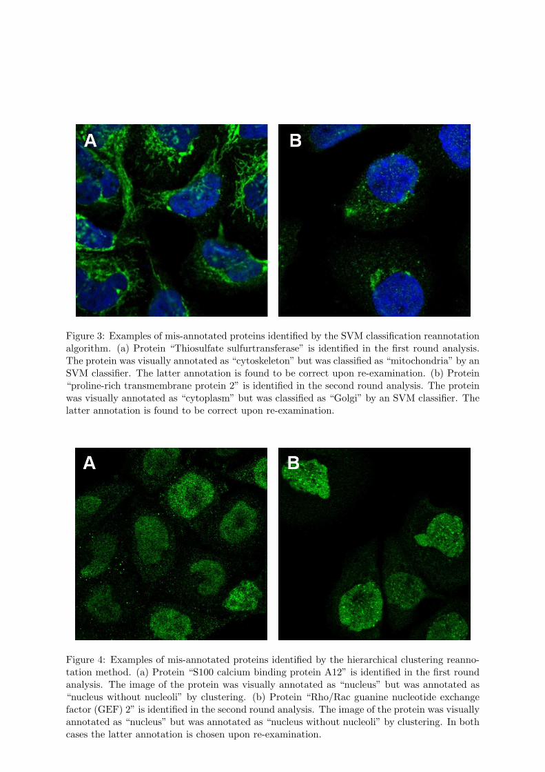
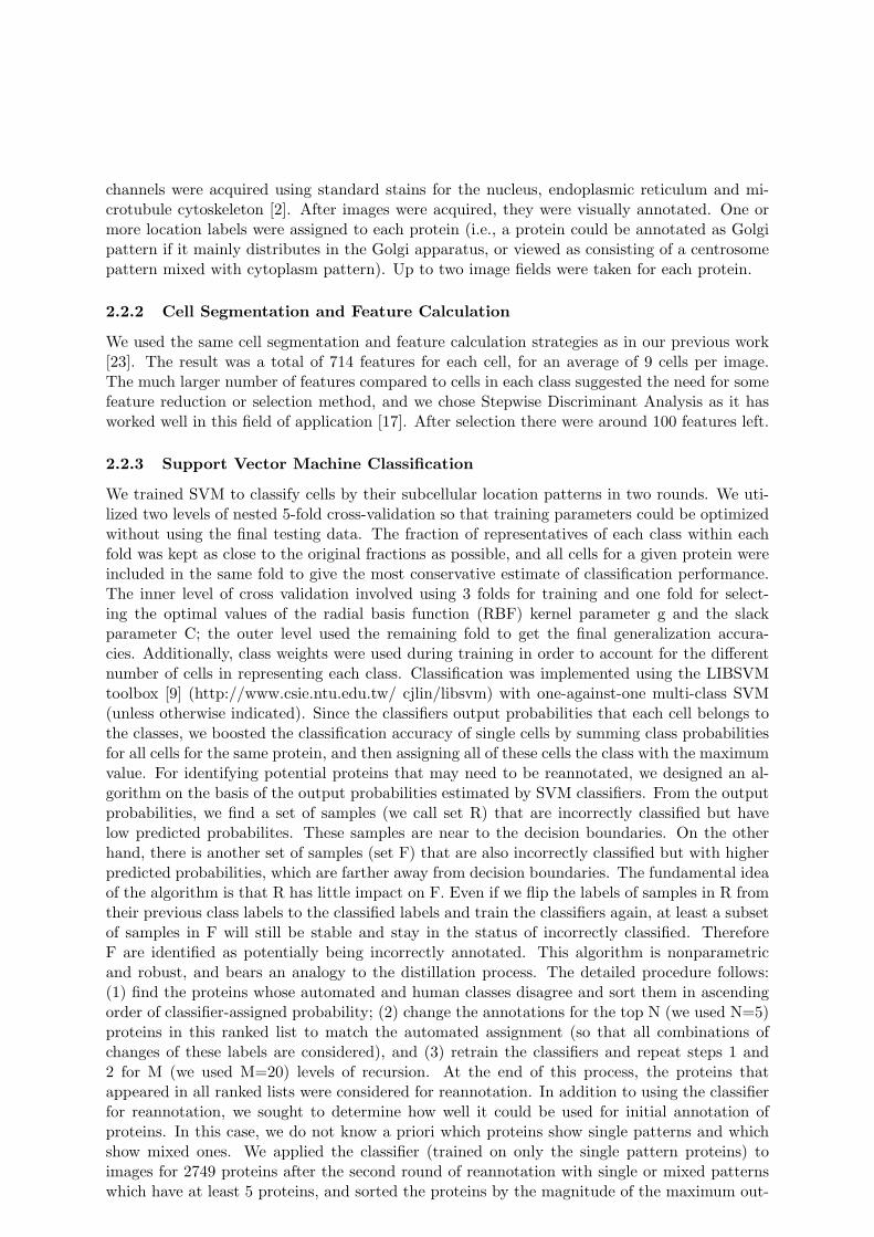
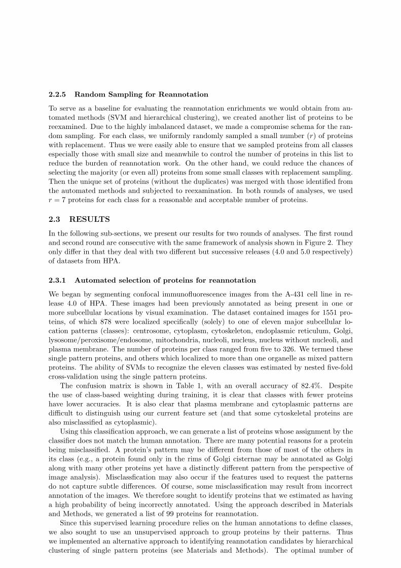
Figure 3: Examples of mis-annotated proteins identified by the SVM classification reannotationalgorithm. (a) Protein “Thiosulfate sulfurtransferase” is identified in the first round analysis.The protein was visually annotated as “cytoskeleton” but was classified as “mitochondria” by anSVM classifier. The latter annotation is found to be correct upon re-examination. (b) Protein“proline-rich transmembrane protein 2” is identified in the second round analysis. The proteinwas visually annotated as “cytoplasm” but was classified as “Golgi” by an SVM classifier. Thelatter annotation is found to be correct upon re-examination.

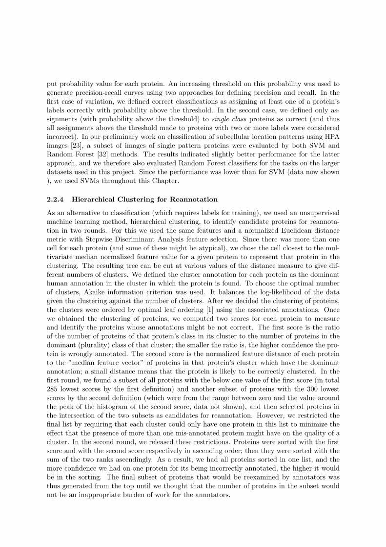
Figure 4: Examples of mis-annotated proteins identified by the hierarchical clustering reanno-tation method. (a) Protein “S100 calcium binding protein A12” is identified in the first roundanalysis. The image of the protein was visually annotated as “nucleus” but was annotated as“nucleus without nucleoli” by clustering. (b) Protein “Rho/Rac guanine nucleotide exchangefactor (GEF) 2” is identified in the second round analysis. The image of the protein was visuallyannotated as “nucleus” but was annotated as “nucleus without nucleoli” by clustering. In bothcases the latter annotation is chosen upon re-examination.

10

whose annotations changed upon reexamination. The reannotation rate for proteins chosenat random was therefore 14/65 = 22%, while the rates for proteins identified by SVM andhierarchical clustering respectively were (21+7+11)/99 = 39% and (2+2)/12 = 33% (the ratefor the combination of the two was 41/106 = 39%). Thus, we observed between 1.5-fold and1.8-fold enrichment in identifying incorrectly annotated proteins above random.

To calculate the statistical significance of reannotation from either SVM or clustering com-pared to that from random sampling, we modeled the number of reannotated proteins as suc-cesses in a binomial distribution. Therefore, the p-value of reannotation from SVM was 1 −binocdf(39, 99, 14/65) = 1.7e−5, from clustering was 1−binocdf(4, 12, 14/65) = 0.095 and fromthe combination of the two was 1 − binocdf(41, 106, 14/65) = 1.9e − 5, where binocdf(X, N, P )represented the cumulative distribution function of binomial distribution at each of the valuesin X (the number of successes) using the corresponding parameters in N (the number of trials)and P (rate of success in each trial). Thus under the significance level α = 0.05, reannotationsfrom SVM and combination are statistically significant while that from clustering is not.

Using the new annotations, we repeated the SVM classification. The overall accuracy im-proved to 86.4% compared with 82.4% in Table 1. This improvement is due directly to thechanges in the annotations of the re-examined proteins, and no improvement in classification ofother proteins is observed.

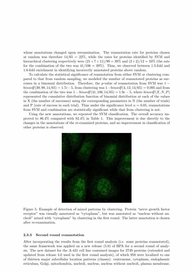
Figure 5: Example of detection of mixed patterns by clustering. Protein “nerve growth factorreceptor” was visually annotated as “cytoplasm”, but was annotated as “nucleus without nu-cleoli” mixed with “cytoplasm” by clustering in the first round. The latter annotation is chosenafter re-examination.

2.3.3 Second round reannotation

After incorporating the results from the first round analysis (i.e. some proteins reannotated),the same framework was applied on a new release (5.0) of HPA for a second round of analy-sis. The new dataset for the A-431 cell line contained images for 2749 proteins (extended andupdated from release 4.0 used in the first round analysis), of which 958 were localized to oneof thirteen major subcellular location patterns (classes): centrosome, cytoplasm, endoplasmicreticulum, Golgi, mitochondria, nucleoli, nucleus, nucleus without nucleoli, plasma membrane,

11

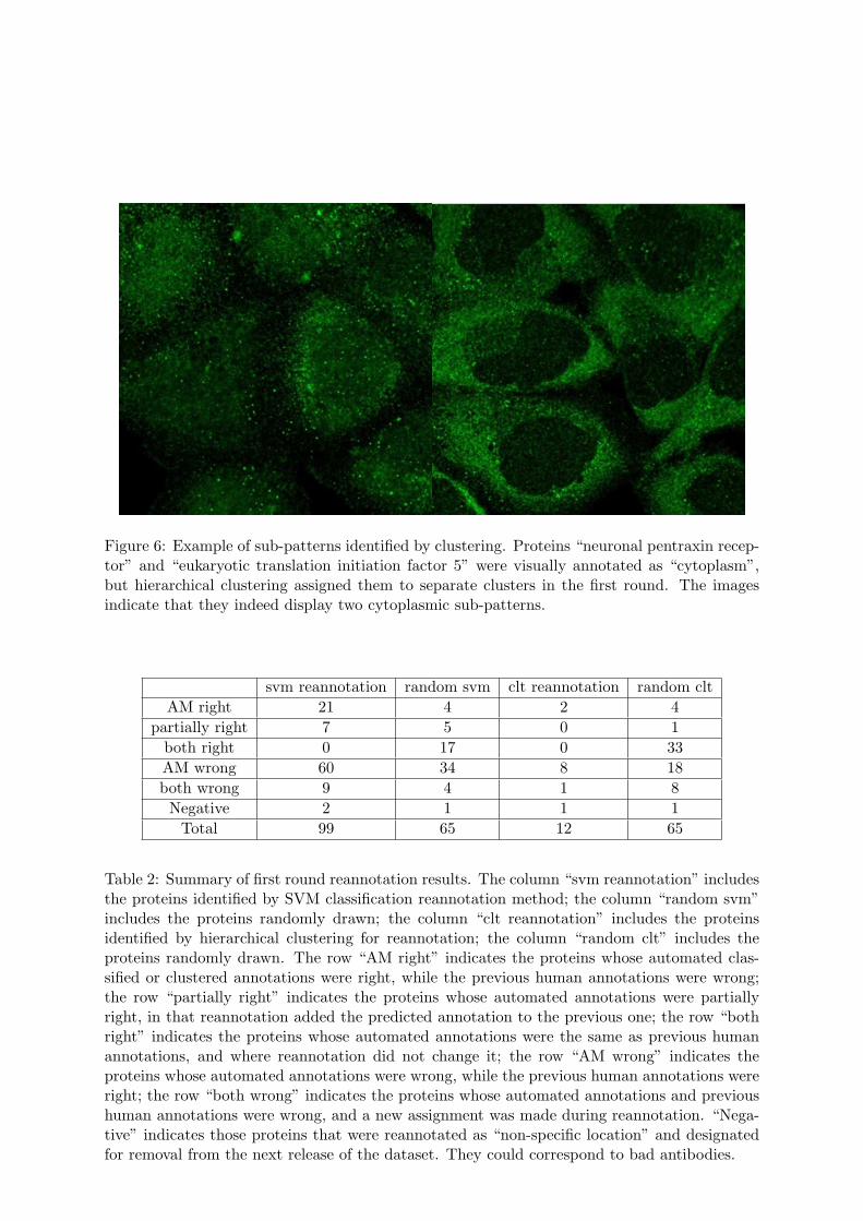
Figure 6: Example of sub-patterns identified by clustering. Proteins “neuronal pentraxin recep-tor” and “eukaryotic translation initiation factor 5” were visually annotated as “cytoplasm”,but hierarchical clustering assigned them to separate clusters in the first round. The imagesindicate that they indeed display two cytoplasmic sub-patterns.

svm reannotation random svm clt reannotation random clt

AM right 21 4 2 4

partially right 7 5 0 1

both right 0 17 0 33

AM wrong 60 34 8 18

both wrong 9 4 1 8

Negative 2 1 1 1

Total 99 65 12 65

Table 2: Summary of first round reannotation results. The column “svm reannotation” includesthe proteins identified by SVM classification reannotation method; the column “random svm”includes the proteins randomly drawn; the column “clt reannotation” includes the proteinsidentified by hierarchical clustering for reannotation; the column “random clt” includes theproteins randomly drawn. The row “AM right” indicates the proteins whose automated clas-sified or clustered annotations were right, while the previous human annotations were wrong;the row “partially right” indicates the proteins whose automated annotations were partiallyright, in that reannotation added the predicted annotation to the previous one; the row “bothright” indicates the proteins whose automated annotations were the same as previous humanannotations, and where reannotation did not change it; the row “AM wrong” indicates theproteins whose automated annotations were wrong, while the previous human annotations wereright; the row “both wrong” indicates the proteins whose automated annotations and previoushuman annotations were wrong, and a new assignment was made during reannotation. “Nega-tive” indicates those proteins that were reannotated as “non-specific location” and designatedfor removal from the next release of the dataset. They could correspond to bad antibodies.

12

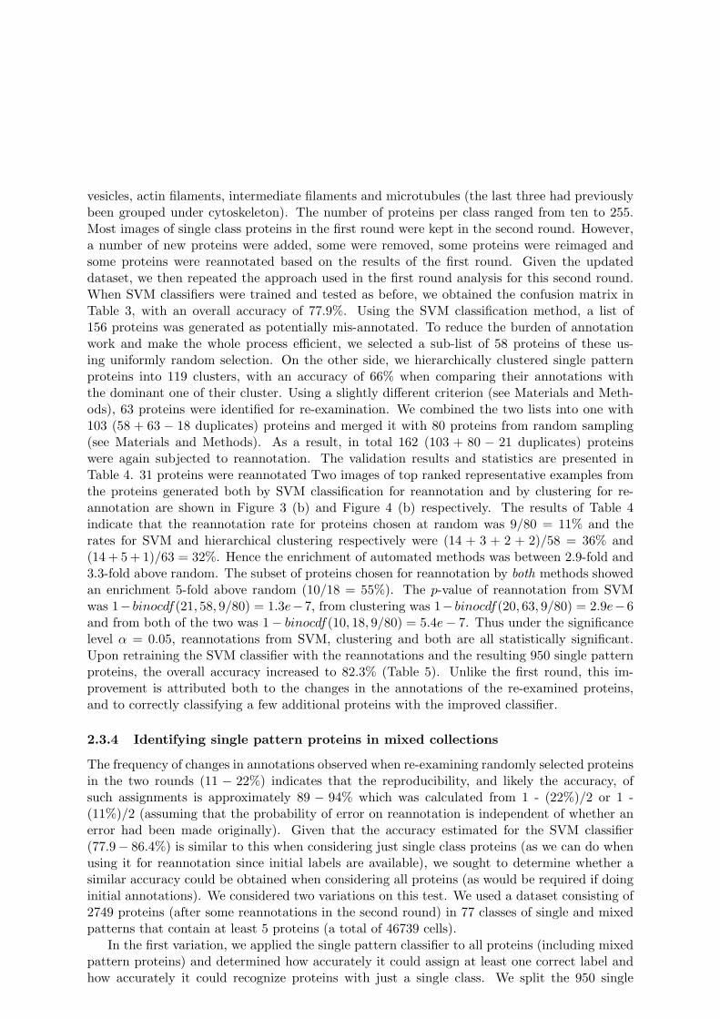
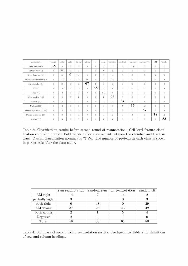
vesicles, actin filaments, intermediate filaments and microtubules (the last three had previouslybeen grouped under cytoskeleton). The number of proteins per class ranged from ten to 255.Most images of single class proteins in the first round were kept in the second round. However,a number of new proteins were added, some were removed, some proteins were reimaged andsome proteins were reannotated based on the results of the first round. Given the updateddataset, we then repeated the approach used in the first round analysis for this second round.When SVM classifiers were trained and tested as before, we obtained the confusion matrix inTable 3, with an overall accuracy of 77.9%. Using the SVM classification method, a list of156 proteins was generated as potentially mis-annotated. To reduce the burden of annotationwork and make the whole process efficient, we selected a sub-list of 58 proteins of these us-ing uniformly random selection. On the other side, we hierarchically clustered single patternproteins into 119 clusters, with an accuracy of 66% when comparing their annotations withthe dominant one of their cluster. Using a slightly different criterion (see Materials and Meth-ods), 63 proteins were identified for re-examination. We combined the two lists into one with103 (58 + 63 − 18 duplicates) proteins and merged it with 80 proteins from random sampling(see Materials and Methods). As a result, in total 162 (103 + 80 − 21 duplicates) proteinswere again subjected to reannotation. The validation results and statistics are presented inTable 4. 31 proteins were reannotated Two images of top ranked representative examples fromthe proteins generated both by SVM classification for reannotation and by clustering for re-annotation are shown in Figure 3 (b) and Figure 4 (b) respectively. The results of Table 4indicate that the reannotation rate for proteins chosen at random was 9/80 = 11% and therates for SVM and hierarchical clustering respectively were (14 + 3 + 2 + 2)/58 = 36% and(14 + 5 + 1)/63 = 32%. Hence the enrichment of automated methods was between 2.9-fold and3.3-fold above random. The subset of proteins chosen for reannotation by both methods showedan enrichment 5-fold above random (10/18 = 55%). The p-value of reannotation from SVMwas 1− binocdf(21, 58, 9/80) = 1.3e−7, from clustering was 1− binocdf(20, 63, 9/80) = 2.9e−6and from both of the two was 1− binocdf(10, 18, 9/80) = 5.4e− 7. Thus under the significancelevel α = 0.05, reannotations from SVM, clustering and both are all statistically significant.Upon retraining the SVM classifier with the reannotations and the resulting 950 single patternproteins, the overall accuracy increased to 82.3% (Table 5). Unlike the first round, this im-provement is attributed both to the changes in the annotations of the re-examined proteins,and to correctly classifying a few additional proteins with the improved classifier.

2.3.4 Identifying single pattern proteins in mixed collections

The frequency of changes in annotations observed when re-examining randomly selected proteinsin the two rounds (11 − 22%) indicates that the reproducibility, and likely the accuracy, ofsuch assignments is approximately 89 − 94% which was calculated from 1 - (22%)/2 or 1 -(11%)/2 (assuming that the probability of error on reannotation is independent of whether anerror had been made originally). Given that the accuracy estimated for the SVM classifier(77.9− 86.4%) is similar to this when considering just single class proteins (as we can do whenusing it for reannotation since initial labels are available), we sought to determine whether asimilar accuracy could be obtained when considering all proteins (as would be required if doinginitial annotations). We considered two variations on this test. We used a dataset consisting of2749 proteins (after some reannotations in the second round) in 77 classes of single and mixedpatterns that contain at least 5 proteins (a total of 46739 cells).

In the first variation, we applied the single pattern classifier to all proteins (including mixedpattern proteins) and determined how accurately it could assign at least one correct label andhow accurately it could recognize proteins with just a single class. We split the 950 single

13

Accuracy% centro. cyto. actin inter. micro. er golgi mitoch. nucleoli nucleus nucleus w/o PM vesicles

Centrosome (16) 38 6 0 0 0 0 19 0 0 13 0 0 25

Cytoplasm (129) 0 90 0 0 1 0 1 3 0 0 0 0 5

Actin filaments (10) 0 60 0 10 0 0 0 10 0 0 0 10 10

Intermediate filaments (9) 0 33 0 33 11 0 0 22 0 0 0 0 0

Microtubules (21) 0 29 0 0 67 5 0 0 0 0 0 0 0

ER (41) 0 20 0 0 0 68 0 10 0 2 0 0 0

Golgi (64) 0 2 0 0 0 0 86 8 0 0 0 0 5

Mitochondria (148) 0 0 0 1 0 0 1 96 0 0 0 0 2

Nucleoli (67) 0 0 0 0 0 0 0 0 87 6 4 0 3

Nucleus (110) 0 1 0 0 0 0 0 0 5 36 58 0 0

Nucleus w/o nucleoli (255) 0 0 0 0 0 0 0 0 2 11 87 0 0

Plasma membrane (17) 0 59 0 0 0 0 0 6 0 6 0 18 12

Vesicles (71) 1 4 0 0 0 1 4 4 0 1 0 0 83

Table 3: Classification results before second round of reannotation. Cell level feature classi-fication confusion matrix. Bold values indicate agreement between the classifier and the trueclass. Overall classification accuracy is 77.9%. The number of proteins in each class is shownin parenthesis after the class name.

svm reannotation random svm clt reannotation random clt

AM right 14 2 14 2

partially right 3 6 0 3

both right 0 48 0 29

AM wrong 37 23 43 42

both wrong 2 1 5 4

Negative 2 0 1 0

Total 58 80 63 80

Table 4: Summary of second round reannotation results. See legend to Table 2 for definitionsof row and column headings.

14

Accuracy% centro. cyto. actin inter. micro. er golgi mitoch. nucleoli nucleus nucleus w/o PM vesicles

Centrosome (16) 31 6 0 0 0 0 19 13 6 6 0 0 19

Cytoplasm (126) 0 94 0 0 0 0 0 2 0 0 0 0 4

Actin filaments (10) 0 40 10 10 0 0 0 10 0 0 0 20 10

Intermediate filaments (12) 0 25 0 42 0 8 0 25 0 0 0 0 0

Microtubules (18) 0 17 0 0 78 6 0 0 0 0 0 0 0

ER (40) 0 13 0 0 0 78 0 10 0 0 0 0 0

Golgi (64) 0 2 0 0 0 0 97 0 0 0 0 0 2

Mitochondria (148) 0 1 0 1 0 1 1 95 0 0 1 0 1

Nucleoli (66) 0 2 0 0 0 0 0 0 88 5 3 0 3

Nucleus (91) 0 0 0 0 0 0 0 0 7 30 64 0 0

Nucleus w/o nucleoli (272) 0 0 0 0 0 0 0 0 1 4 94 0 0

Plasma membrane (14) 0 50 0 0 0 0 0 7 0 7 0 29 7

Vesicles (73) 0 5 0 0 0 0 1 7 0 3 1 0 82

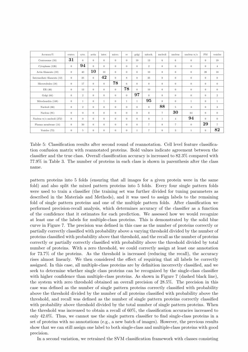
Table 5: Classification results after second round of reannotation. Cell level feature classifica-tion confusion matrix with reannotated proteins. Bold values indicate agreement between theclassifier and the true class. Overall classification accuracy is increased to 82.3% compared with77.9% in Table 3. The number of proteins in each class is shown in parenthesis after the classname.

pattern proteins into 5 folds (ensuring that all images for a given protein were in the samefold) and also split the mixed pattern proteins into 5 folds. Every four single pattern foldswere used to train a classifier (the training set was further divided for tuning parameters asdescribed in the Materials and Methods), and it was used to assign labels to the remainingfold of single pattern proteins and one of the multiple pattern folds. After classification weperformed precision-recall analysis, which determines accuracy of the classifier as a functionof the confidence that it estimates for each prediction. We assessed how we would recognizeat least one of the labels for multiple-class proteins. This is demonstrated by the solid bluecurve in Figure 7. The precision was defined in this case as the number of proteins correctly orpartially correctly classified with probability above a varying threshold divided by the number ofproteins classified with probability above that threshold, and the recall as the number of proteinscorrectly or partially correctly classified with probability above the threshold divided by totalnumber of proteins. With a zero threshold, we could correctly assign at least one annotationfor 73.7% of the proteins. As the threshold is increased (reducing the recall), the accuracyrises almost linearly. We then considered the effect of requiring that all labels be correctlyassigned. In this case, all multiple-class proteins are by definition incorrectly classified, and weseek to determine whether single class proteins can be recognized by the single-class classifierwith higher confidence than multiple-class proteins. As shown in Figure 7 (dashed black line),the system with zero threshold obtained an overall precision of 28.5%. The precision in thiscase was defined as the number of single pattern proteins correctly classified with probabilityabove the threshold divided by the number of all proteins classified with probability above thethreshold, and recall was defined as the number of single pattern proteins correctly classifiedwith probability above threshold divided by the total number of single pattern proteins. Whenthe threshold was increased to obtain a recall of 60%, the classification accuracies increased toonly 42.0%. Thus, we cannot use the single pattern classifier to find single-class proteins in aset of proteins with no annotations (e.g., a new batch of images). However, the previous resultsshow that we can still assign one label to both single-class and multiple-class proteins with goodprecision.

In a second variation, we retrained the SVM classification framework with classes consisting

15

of all label combinations observed for both single and mixed patterns (there were 77 uniqueclasses), explicitly giving it the ability to recognize single class proteins in the presence ofmultiple-class proteins. The overall accuracy of the classifier for all patterns was only 45.4%,illustrating the difficulty of assigning all labels correctly. We therefore asked how well the singleprotein classes could be recognized. The precision-recall curve for this task is shown as thedotted red line in Figure 7. The precision was defined as the number of single pattern proteinscorrectly classified with probability above the threshold divided by the number of proteinsclassified as single pattern with probability above the threshold, and recall as the number ofsingle pattern proteins correctly classified with probability above the threshold divided by thetotal number of single pattern proteins. At a zero threshold, the accuracy for recognizing singleclass proteins was found to be 64.0%. At a threshold corresponding to 17% recall, the precisionimproved to 90.1%. Thus single class proteins can be correctly recognized with reasonableaccuracy by a classifier trained on either single or multiple-class proteins.

Figure 7: Precision-recall curves for protein annotations for single and multi-class classifiers. Forthe solid blue and dashed black line, we predicted the annotations of single pattern and mixedpattern proteins used a classifier trained with only single pattern proteins. For the solid blueline, annotations were considered correct if one of the annotations of one protein was predicted.For the dashed black line, only recognition of single pattern proteins was considered correct.For the dotted red line, a classifier trained on both single and mixed pattern proteins was used,but only the accuracy of recognizing single pattern proteins was assessed.

2.4 DISCUSSION

Microscopy images are rich sources of information about cell structure and function for systemsbiology. We have presented a framework to classify proteome-scale collections of proteins con-taining complex subcellular location patterns, and our classifier provides performance similarto human annotation on single-class proteins.

The only prior work on the automated classification of proteins using HPA confocal im-munofluorescence images was described by Newberg et al. [23]. In this Chapter, we obtain

16

similar classification accuracies on single-class proteins but analyze many more proteins andpatterns. The cytoplasm pattern, which has the second largest number of proteins, was addedand introduces some confusion with other patterns because of non-specific staining over thecell. The nucleus pattern was split into nucleus pattern and nucleus without nucleoli pattern toprovide more detailed annotations, notwithstanding the two are highly blended in the stainingand are difficult to distinguish visually in many images. The small class of cytoskeleton was alsoeven split into three further patterns of actin, intermediate filaments and microtubules whichreduces the number of training images available for each. Nonetheless, good classification ac-curacies were maintained, which represents a significant advance over our prior work. However,the accuracies are not yet high enough to replace human annotators. In the future, we plan toimplement new features specific for the centrosome pattern, and hope to add features for betterdiscriminating the cytoskeleton and plasma membrane patterns from the cytoplasm pattern.

One of the main novelties we describe in this Chapter is the introduction of approachesto identify possible mis-annotated proteins, derived from SVM classification and hierarchicalclustering, and the demonstration that they could identify proteins needing reannotation at arate higher than random. Our results show that selecting proteins using both schemes achieveshigher yield of reannotated proteins than either of them alone or in combination. We planto continue cycles of reannotation, and to incorporate the automated system in the annotationpipeline. Note that in this Chapter we only provide results for the A-431 cell line, but the wholeframework introduced here can be applied to other cell lines, such as U-2OS and U-251MG. Asa matter of fact, some preliminary results have already been obtained (data not shown; includedin Reproducible Research Archive as described in Materials and Methods). We hope therebyto maximize the accuracy of reported annotations in the Human Protein Atlas. We anticipatethat a similar approach may be applied to other proteome-scale image collections.

The dataset used in this Chapter contains 2D, static confocal images of fixed cells fromHPA. In the future, the temporal dynamics of the variations of protein subcellular locationpatterns and the evolution over the course of stem cell differentiation can be explored by ourframework as datasets become available.

Another novel aspect of this work is the results on full or partial recognition of mixed patternproteins. Our results highlight the difficulty of handling these patterns. The main problem isthat the features are affected by the degree of mixture. This is unlike the case for tasks likedocument classification, in which the addition of a second topic associated with new words doesnot alter the detection of words associated with the first topic. It is also unlike the case inmany natural scene images in which adding a dog to an image of a cat does not change the localfeatures associated with the cat. In these cases, a number of multiclass learning strategies havebeen successfully used. For protein patterns consisting of vesicular objects, we have used similarmethods to show that the frequency of object types can be used to estimate mixing betweenpatterns (using both supervised [28] and unsupervised [12] approaches). Unfortunately, thisapproach does not generalize to mixtures involving non-vesicular proteins, and preliminarywork indicates that local features such as SIFT [22] also do not perform well in that case.

17

3 Protein Subcellular Location Pattern Classification in Cellu-lar Images Using Latent Discriminative Models

2

3.1 INTRODUCTION

The fully automated recognition of protein subcellular location patterns requires as high ac-curacy as possible for the classification framework. In this Chapter, we has improved theclassification performance on the basis of region-based (or patch-based) computer vision meth-ods which incorporates much more local protein distribution information compared with celllevel features in Chapter 2.

We in fact aim at learning from the data the dependencies among features, cell components,and the protein pattern classes into which the images have been divided. To accomplish this,we build two graphical models with latent variables to capture the cell components (invisibleor hidden) and these dependencies. These two models are based on logistic regression [5]. Thefirst model, called hidden logistic regression (HLR), introduces the concept of component as alatent variable into the simple logistic regression, so that the protein and the component candetermine the expressed features together. The second model, called hidden conditional randomfield (HCRF), further introduces spatial dependencies among components at different locationswithin cell as in conditional random field (CRF) developed by [20]. These two models cancapture the components’ influence on the expressed features and their spatial configurations,thus improving our ability to recognize the patterns.

We use gradient based methods to estimate the models’ parameters. We show that thegradients depend on the marginal probabilities on the nodes and edges in the model. For HLR,this computation is easy. But for the HCRF model, inferences for these marginals cannot bedone exactly. To address this difficulty in inference, we propose to remove certain edges inthe HCRF model so that the component variables are “clustered”. By doing this, the exactinference is greatly accelerated while most of the local interactions between cell components canbe retained.

The effectiveness of both the HLR and HCRF models are tested on synthetic data and realHPA images. We show that using latent variables to model the components can enhance theclassification accuracy. Furthermore, spatial dependencies can significantly improve the perfor-mance. With the proposed models, we are able to achieve the best classification performanceon this task to our knowledge.

The rest of the Chapter is organized as below. First we describe the data set and define theproblem we try to solve in Section 3.2. Then the proposed classification methods are describedin Section 3.3. Experimental results are shown in Section 3.4 on both synthetic simulations andreal cellular images. In Section 3.5 we discuss some related work and summarize this Chapter.

3.2 BACKGROUND

3.2.1 Data Set

Similarly to the Chapter 2, we also used HPA images. For the experiments in this Chapter,we chose a subset of the HPA images consisting of 1882 images of 9423 proteins from one of13 classes: centrosome, cytoplasm, actin filaments, intermediate filaments, microtubules, ER,Golgi, mitochondria, nuclei, nucleus without nucleoli, nucleoli, plasma membrane, and vesicles.

2This work is a collaboration with Liang Xiong (Machine Learning Department at Carnegie Mellon Univer-sity), and is adapted from “Protein subcellular location pattern classification in cellular images using latentdiscriminative models” by Jieyue Li, Liang Xiong, Jeff Schneider, and Robert F. Murphy which appeared inBioinformatics 28:i32-i39 (2012).

3A little more proteins were reannotated after Chapter 2

18

To preprocess the image data, we first used the seeded watershed method to segment theimage fields into single cells [23]. After that, for every cell we randomly select 50 regions ofsize 41 × 41 pixels, each of which must contain some of the stained protein signal (i.e. notempty). The size is chosen so that an individual region captures fine enough information aboutthe specific component in it, and the number of regions is chosen so that most of the area ofthe cell is covered while it is computationally feasible to solve the problem.

To extract features from the sampled regions, we computed various subcellular location fea-tures (SLF) according to [23] on individual channels separately as well as on the combinationsof different channels. These features essentially characterize the appearance, the texture infor-mation, the multi-resolution aspect, and the spatial distribution of different cell components inthe image regions. After feature extraction and removing bad regions and cells, we have 15990cells, containing 799015 regions with 2538 dimensional features.

3.2.2 Problem Definition

To begin with, we give a brief re-statement of the problem. The data we have is a set of cellularimages. For each small rectangular (square) region in those images, we can observe some vectorof features, and we know the class of the protein stained in this cell and region. Given thesedata, our goal is to train a model that can classify the distribution pattern of the protein stainedin unlabeled images.

We introduce some notations here. Suppose there are N cells containing M image regions,T types of cell components, and K classes. The features we have for region m is Fm ∈ R

DF ,where DF stands for the size of feature. For this region, we have a label Cm indicating the classof the stained protein.

3.3 METHODS

3.3.1 The Latent Discriminative Models

We take a discriminative approach and design models to solve the classification problem directly.The most straightforward way of modeling is to let the region’s protein class label Cm

directly determine the features Fm we observe in that region. We can describe this simplemodel using the undirected graphical model in Figure 8.

Cm FmM

Figure 8: The Logistic Regression (LR) model for regions. Fm are the features and Cm is thelabel.

We adopt a discriminative approach here. Instead of modeling the joint probability ofthe labels and features, we directly characterize the probabilities of labels conditioned on thefeatures, since our focus here is prediction. Based on this principle, we can use a log-linearmodel to realize the model in Figure 8 as follows:

P (Cm = k|Fm, Θ) ∝ exp(

wTk Fm

)

(1)

where the parameter set Θ contains w1, · · · , wK , one for each class, and the footnote T in allequations stands for transpose. We can see that this model is in fact Logistic Regression (LR)for multi-class problems. After training, the LR model is able to predict the class label for eachtest region, based on which cell-level and protein-level predictions can be obtained by voting.This simple LR model is our starting point.

19

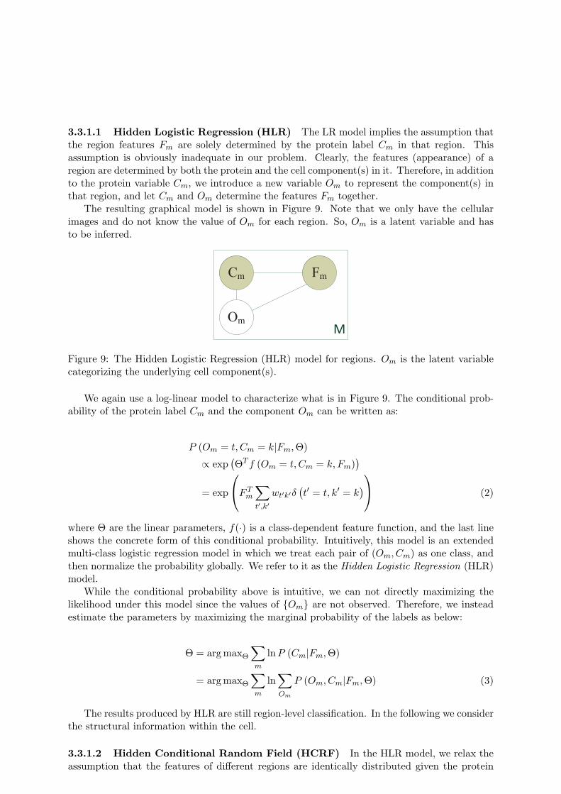
3.3.1.1 Hidden Logistic Regression (HLR) The LR model implies the assumption thatthe region features Fm are solely determined by the protein label Cm in that region. Thisassumption is obviously inadequate in our problem. Clearly, the features (appearance) of aregion are determined by both the protein and the cell component(s) in it. Therefore, in additionto the protein variable Cm, we introduce a new variable Om to represent the component(s) inthat region, and let Cm and Om determine the features Fm together.

The resulting graphical model is shown in Figure 9. Note that we only have the cellularimages and do not know the value of Om for each region. So, Om is a latent variable and hasto be inferred.

M

Cm Fm

Om

Figure 9: The Hidden Logistic Regression (HLR) model for regions. Om is the latent variablecategorizing the underlying cell component(s).

We again use a log-linear model to characterize what is in Figure 9. The conditional prob-ability of the protein label Cm and the component Om can be written as:

P (Om = t, Cm = k|Fm, Θ)

∝ exp(

ΘT f (Om = t, Cm = k, Fm))

= exp

F Tm

∑

t′,k′

wt′k′δ(

t′ = t, k′ = k)

(2)

where Θ are the linear parameters, f(·) is a class-dependent feature function, and the last lineshows the concrete form of this conditional probability. Intuitively, this model is an extendedmulti-class logistic regression model in which we treat each pair of (Om, Cm) as one class, andthen normalize the probability globally. We refer to it as the Hidden Logistic Regression (HLR)model.

While the conditional probability above is intuitive, we can not directly maximizing thelikelihood under this model since the values of {Om} are not observed. Therefore, we insteadestimate the parameters by maximizing the marginal probability of the labels as below:

Θ = arg maxΘ

∑

m

lnP (Cm|Fm, Θ)

= arg maxΘ

∑

m

ln∑

Om

P (Om, Cm|Fm, Θ) (3)

The results produced by HLR are still region-level classification. In the following we considerthe structural information within the cell.

3.3.1.2 Hidden Conditional Random Field (HCRF) In the HLR model, we relax theassumption that the features of different regions are identically distributed given the protein

20

class label, and let one protein class be expressed differently at different parts of the cell. Butwe are still assuming that the regions are independent of each other. However, in fact we knowthat there are spatial dependencies among the components. For example, the Golgi complex isusually located near the nucleus. So when we see the nucleus, which is easy to recognize, wehave some clue that the Golgi complex will be nearby. This type of reasoning is frequently usedwhen human experts try to classify a protein pattern. Our next step is trying to emulate thisprocess and capture the spatial dependencies among the components.

Unlike previous sections where we focus on regions, here we treat cells as the units inclassification. For cell n, we let Mn be the number of regions in it. Further, Fn/Gn, Cn are thefeatures and the label for the cell n, and On,m is the component(s) in the mth region of the celln.

The new model extends HLR described in Section 3.3.1.1 by allowing the components in thesame cell to interact with each other. The graphical model that captures all the dependenciesis shown in Figure 10.

On,2

Cn

On,1

On,3N

Fn, Gn

Figure 10: The Hidden Conditional Random Field (HCRF) model for cells. All the components{On,m} are latent variables.

As before, we use log-linear models to characterize the dependencies between variables, asin conditional random field (CRF) by [20]. The conditional probability of the protein label andcomponent is as follows:

P (Cn, On|Fn, Θ) ∝ exp(Ψ) (4)

Ψ =∑

i∈Nn

ΘTf f (Cn, On,i, Fn)

+∑

(i,j)∈En

ΘTg g (Cn, On,i, On,j , Fn)

=∑

i

F Tn,i

∑

t′,k′

wt′k′δ(

On,i = t′, Cn = k′)

+∑

(i,j)

GTn,ij

∑

s′,t′

vs′t′δ(

On,i = s′, On,j = t′)

, (5)

where N , E are the node and edge sets. In this model, the parameter set Θ includes {wtk} and{vst}. The association features Fn,i ∈ R

DF provide evidence for an individual region i, andthe interaction feature Gn,ij ∈ R

DG provides evidence for the dependency between a regionpair (i, j). {wtk} define the potential on each region, and {vst} define the potential for pairsof regions. As before, the components On are not observed. We call this model the HiddenConditional Random Field (HCRF).

To learn this model, we also need to maximize the marginal likelihood of the labels Cn.That is, our goal is to solve the problem in the following:

21

Θ = arg maxΘ

∑

n

lnP (Cn|Fn, Θ)

= arg maxΘ

∑

n

ln∑

On

P (Cn, On|Fn, Θ). (6)

Note that unlike LR and HLR, HCRF is able to produce cell-level prediction directly.

3.3.2 Learning

In this section, we describe how to learn the proposed HLR and HCRF models, and use themfor prediction.

3.3.2.1 Training We use gradient based optimization to train the parameters of the HLRand HCRF models. As shown in Section 3.3.1, the goal of learning is to maximize the marginalprobability of the data:

Θ = arg maxΘ

∑

n

Ln,

Ln = ln∑

On

P (Cn, On|Fn, Θ) (7)

In log-linear models, the conditional probabilities in general can be written as:

P (Cn, On|Fn, Θ) ∝ exp(

ΘT f (Cn, On, Fn))

= exp (Ψ (Cn, On, Fn, Θ))

= exp(Ψn). (8)

Meanwhile, the marginal of the label Cn can be written as follows:

P (Cn|Fn, Θ) =∑

On

P (Cn, On|Fn, Θ) =

∑

Onexp (Ψn)

Zn

(9)

Zn =∑

Cn

∑

On

exp (Ψn) (10)

By taking the derivative of Ln with respect to some parameter θ, the following results canbe derived:

∂ log∑

Onexp (Ψn)

∂θ=∑

On

P (On|Cn, Fn, Θ)∂Ψn

∂θ, (11)

∂ log Zn

∂θ=∑

Cn,On

P (Cn, On|F, Θ)∂Ψn

∂θ, (12)

∂Ln

∂θ=

∂ log∑

Onexp (Ψn)

∂θ−

∂Zn

∂θ

=∑

On

P (On|Cn, Fn, Θ)∂Ψn

∂θ

−∑

Cn,On

P (Cn, On|F, Θ)∂Ψn

∂θ. (13)

22

From Eq (13), it is easy to obtain the derivative for any parameter in HLR and HCRF. Herewe omit the details and only show the final results.

For the HLR model, the derivatives are

∂Lm

∂wtk

= Fm

(

P (Om = t|Cm, Fm, Θ) δ (Cm = k)

−P (Om = t, Cm = k|Fm, Θ)

)

(14)

For the HCRF model, the derivatives are

∂Ln

∂wtk

=∑

i∈Nn

Fn,i

(

P (On,i = t|Cn, Fn, Θ) δ (Cn = k)

−P (On,i = t, Cn = k|Fn, Θ)

)

(15)

∂Ln

∂vst

=∑

(i,j)∈En

Gn,ij

(

P (On,i = s, On,j = t|Cn, Fn, Θ)

−P (On,i = s, On,j = t|Fn, Θ)

)

(16)

Given these results, we can use gradient based optimizers to train the parameters by maxi-mizing the marginal likelihood of the data. For example, we can use L-BFGS [25] or stochasticgradient descent [7]. Note that the key quantities required to calculate these gradients are themarginal probabilities in the forms of P (O|C, F ) and P (C, O|F ).

3.3.3 Inference

In Section 3.3.2.1, we have derived that in order to apply gradient based learning we need tofirst calculate the marginal probabilities in the forms of P (O|C, F ) and P (C, O|F ). Therefore,inference algorithms are necessary.

For the HLR model, inference is straightforward since the number of terms in the partitionfunction is only T × K. We can easily enumerate all of them to get the exact values of thosemarginal probabilities. Given the exact gradients and the objective values, we apply L-BFGSto learn the HLR model.

For the HCRF model, the inference problem becomes intractable because of the dependencestructure of the graphical model. Brute force is infeasible since the partition function containsK × TM terms, where M is the number of regions in one cell. Other exact methods such asvariable elimination [18] are also not viable because the nodes can be densely connected andtherefore the tree-width [18] of the graph, which determines the complexity of inference, can bevery large. Therefore, we need approximate methods.

Unfortunately, classical approximate inference methods are difficult to apply here. For exam-ple, mean field approximation [18] is not applicable because we need the marginal probabilitieson edges, which are not available from a completely factorized mean field distribution. Thechoice of belief propagation (BP) [26] seems reasonable considering the forms of derivatives inEq (15) because it provides all the marginal probabilities we need. However, the HCRF modelcontains numerous small loops like “C-O-O” and “O-O-O” in Figure 10, which make the BPalgorithm inaccurate or even non-convergent. Moreover, the approximate inference result willprevent the marginal likelihood from being optimized efficiently, due to the fact that we cannotevaluate the objective value correctly.

To solve these problems, we propose to use an approximate model and exact inference,as opposed to using an exact model and approximate inference. Concretely, we first reducethe tree-width of the model and then use variable elimination for inference. We partition thelatent ’O’ nodes of HCRF into small clusters, then the tree-width is equal to the largest clustersize. For example, given that a cell contains 50 components in regions, we can partition thesecomponents into 10 clusters of size 5 based on their spatial locations in the cell. Then, we

23

remove the ’O-O’ edges that cross cluster boundaries, while still keeping all the ’C-O’ edges.By doing this, the tree-width of the model is always limited to a small number regardless of thetotal number of components (regions), making exact inference by variable elimination tractable.

An illustration of this process is shown in Figure 11. We can see that by making thissimplification of model, we lose a few edges, but most of the important local interactions betweenregions are kept. In return, the inference and learning of the simplified model become efficient.Suppose there are M regions in one cell and we partition them into clusters of size s. Then afterthe partition, inference can be done in O(M

sKT s). Note that now the complexity grows only

linearly with the number of regions. However it still grows exponentially with the cluster sizes, which therefore cannot be large. Note that when s = 1, the HCRF degenerates into HLR.

Figure 11: An illustration of how to simply HCRF for tractable exact inference. Each noderepresents an ’O’ node in HCRF.

In summary, we used a “Expectation-Maximization” style to learn the parameters. Weiteratively did inference in section 3.3.3 (with initially random parameters) and likelihood max-imization in section 3.3.2.1.

3.3.4 Implementation

To construct the interaction graphs of HCRF among the components within the same cell, weadd edges between components and their nearest neighbors. In this Chapter we always use the3 nearest neighbors to build the interaction graph. Currently, the feature G on each edge inHCRF is just the distance between the centers of two regions. In the future we may add moredescriptive features for the edges.

Since we have adopted the “approximate model, exact inference” approach, both the gradientand objective value of the data likelihood can be computed exactly, making the optimizationstraightforward. Here we use L-BFGS to maximize the marginal likelihood due to its fastconvergence and low memory consumption.

It should be pointed out that HCRF has a large number of parameters. In order to avoidoverfitting and enhance the generalization ability, we regularize the L2-norm of the parametersas in ridge regression with a penalization parameter λ. This part is straightforward and detailsare omitted.

Since the time required to infer the HCRF model grows exponentially with the cluster sizeinto which regions are grouped, we set the cluster size to 5 with trade-off between speed andapproximation accuracy. With this setting and T = 3, inference took approximately 20 hours

24

on one 2.40 GHz 64-bit processor for the HCRF model. The HLR model took about 10 minuteswhen T = 3.

3.4 RESULTS

In this section, we show the performance of the proposed methods on both synthetic data andreal HPA images.

3.4.1 Simulation

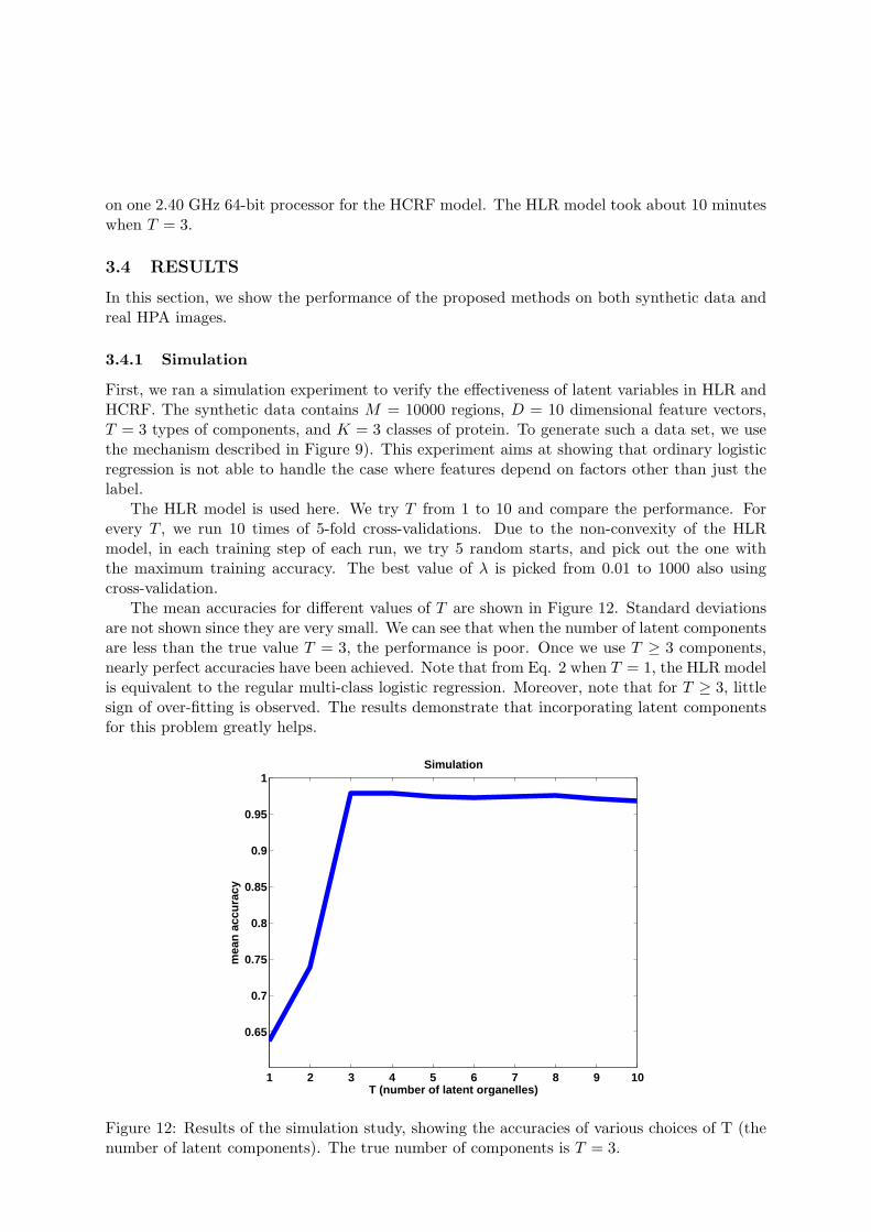
First, we ran a simulation experiment to verify the effectiveness of latent variables in HLR andHCRF. The synthetic data contains M = 10000 regions, D = 10 dimensional feature vectors,T = 3 types of components, and K = 3 classes of protein. To generate such a data set, we usethe mechanism described in Figure 9). This experiment aims at showing that ordinary logisticregression is not able to handle the case where features depend on factors other than just thelabel.

The HLR model is used here. We try T from 1 to 10 and compare the performance. Forevery T , we run 10 times of 5-fold cross-validations. Due to the non-convexity of the HLRmodel, in each training step of each run, we try 5 random starts, and pick out the one withthe maximum training accuracy. The best value of λ is picked from 0.01 to 1000 also usingcross-validation.

The mean accuracies for different values of T are shown in Figure 12. Standard deviationsare not shown since they are very small. We can see that when the number of latent componentsare less than the true value T = 3, the performance is poor. Once we use T ≥ 3 components,nearly perfect accuracies have been achieved. Note that from Eq. 2 when T = 1, the HLR modelis equivalent to the regular multi-class logistic regression. Moreover, note that for T ≥ 3, littlesign of over-fitting is observed. The results demonstrate that incorporating latent componentsfor this problem greatly helps.

1 2 3 4 5 6 7 8 9 10

0.65

0.7

0.75

0.8

0.85

0.9

0.95

1

T (number of latent organelles)

mea

n a

ccu

racy

Simulation

Figure 12: Results of the simulation study, showing the accuracies of various choices of T (thenumber of latent components). The true number of components is T = 3.

25

3.4.2 HPA Protein Classification

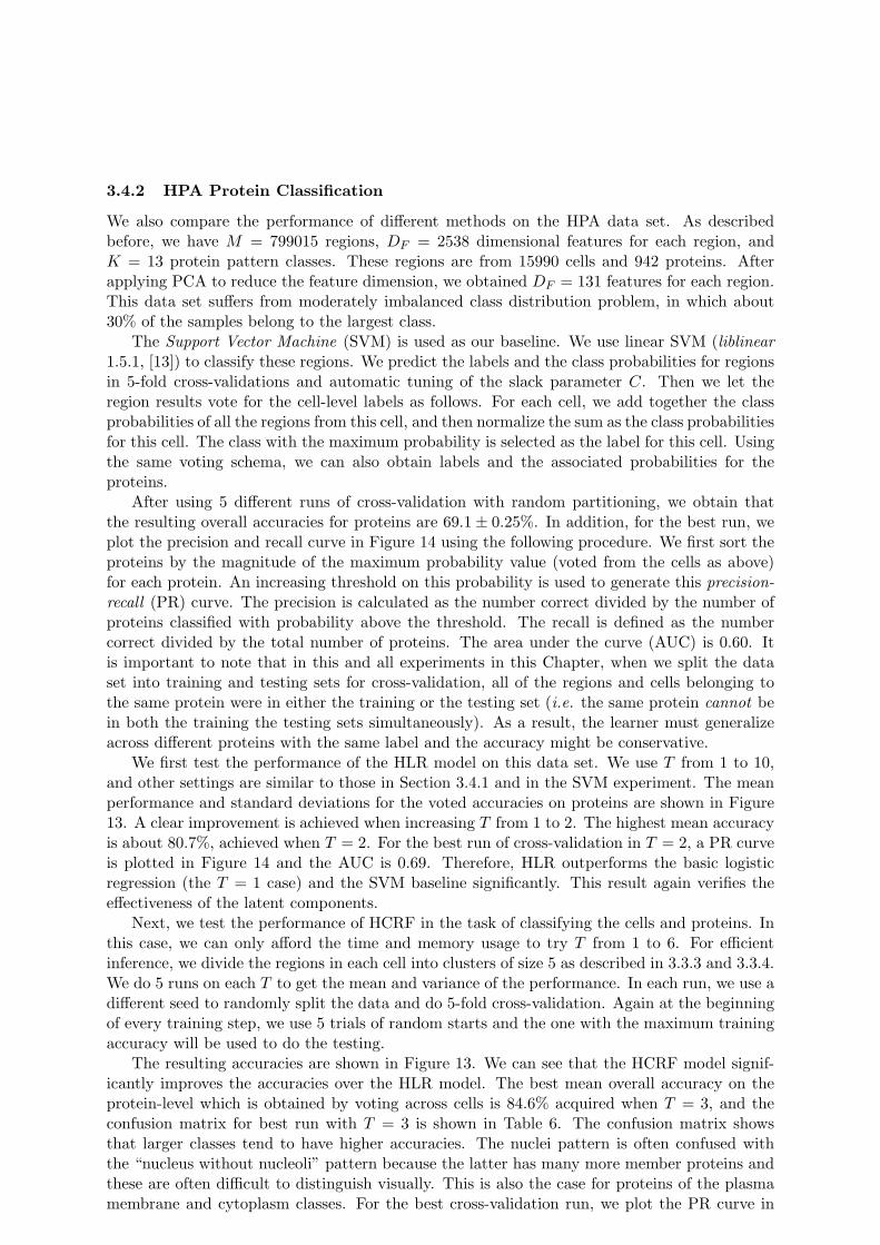
We also compare the performance of different methods on the HPA data set. As describedbefore, we have M = 799015 regions, DF = 2538 dimensional features for each region, andK = 13 protein pattern classes. These regions are from 15990 cells and 942 proteins. Afterapplying PCA to reduce the feature dimension, we obtained DF = 131 features for each region.This data set suffers from moderately imbalanced class distribution problem, in which about30% of the samples belong to the largest class.

The Support Vector Machine (SVM) is used as our baseline. We use linear SVM (liblinear1.5.1, [13]) to classify these regions. We predict the labels and the class probabilities for regionsin 5-fold cross-validations and automatic tuning of the slack parameter C. Then we let theregion results vote for the cell-level labels as follows. For each cell, we add together the classprobabilities of all the regions from this cell, and then normalize the sum as the class probabilitiesfor this cell. The class with the maximum probability is selected as the label for this cell. Usingthe same voting schema, we can also obtain labels and the associated probabilities for theproteins.

After using 5 different runs of cross-validation with random partitioning, we obtain thatthe resulting overall accuracies for proteins are 69.1 ± 0.25%. In addition, for the best run, weplot the precision and recall curve in Figure 14 using the following procedure. We first sort theproteins by the magnitude of the maximum probability value (voted from the cells as above)for each protein. An increasing threshold on this probability is used to generate this precision-recall (PR) curve. The precision is calculated as the number correct divided by the number ofproteins classified with probability above the threshold. The recall is defined as the numbercorrect divided by the total number of proteins. The area under the curve (AUC) is 0.60. Itis important to note that in this and all experiments in this Chapter, when we split the dataset into training and testing sets for cross-validation, all of the regions and cells belonging tothe same protein were in either the training or the testing set (i.e. the same protein cannot bein both the training the testing sets simultaneously). As a result, the learner must generalizeacross different proteins with the same label and the accuracy might be conservative.

We first test the performance of the HLR model on this data set. We use T from 1 to 10,and other settings are similar to those in Section 3.4.1 and in the SVM experiment. The meanperformance and standard deviations for the voted accuracies on proteins are shown in Figure13. A clear improvement is achieved when increasing T from 1 to 2. The highest mean accuracyis about 80.7%, achieved when T = 2. For the best run of cross-validation in T = 2, a PR curveis plotted in Figure 14 and the AUC is 0.69. Therefore, HLR outperforms the basic logisticregression (the T = 1 case) and the SVM baseline significantly. This result again verifies theeffectiveness of the latent components.

Next, we test the performance of HCRF in the task of classifying the cells and proteins. Inthis case, we can only afford the time and memory usage to try T from 1 to 6. For efficientinference, we divide the regions in each cell into clusters of size 5 as described in 3.3.3 and 3.3.4.We do 5 runs on each T to get the mean and variance of the performance. In each run, we use adifferent seed to randomly split the data and do 5-fold cross-validation. Again at the beginningof every training step, we use 5 trials of random starts and the one with the maximum trainingaccuracy will be used to do the testing.

The resulting accuracies are shown in Figure 13. We can see that the HCRF model signif-icantly improves the accuracies over the HLR model. The best mean overall accuracy on theprotein-level which is obtained by voting across cells is 84.6% acquired when T = 3, and theconfusion matrix for best run with T = 3 is shown in Table 6. The confusion matrix showsthat larger classes tend to have higher accuracies. The nuclei pattern is often confused withthe “nucleus without nucleoli” pattern because the latter has many more member proteins andthese are often difficult to distinguish visually. This is also the case for proteins of the plasmamembrane and cytoplasm classes. For the best cross-validation run, we plot the PR curve in

26

Figure 14 which has an AUC of 0.82. From the figure, we can see that if we increase thethreshold to have recall of about 60%, the precision is about 95%.

0 2 4 6 8 10 120.72

0.74

0.76

0.78

0.8

0.82

0.84

0.86

Number of latent variables T

Cro

ss−

valid

atio

n ac

cura

cies

on

prot

eins

HLRHCRF

Figure 13: Classification accuracies on HPA proteins by HLR and HCRF. These accuracies areobtained from cell-level results by probability voting.

Since the HCRF with T ≥ 2 outperforms the one with T = 1, we can conclude that thelatent components and spatial dependencies introduced in HCRF are indeed useful.

Note that the overall accuracy appears to saturate at around 84% in Figure 13. We haveestimated that the overall accuracy of human annotation of these labels in other work is about90% (see section 2.3.4 in Chapter 2), which our classification accuracy approaches. Moreover,any errors in labeling by human experts may result in confusion when used for training theclassifiers. Therefore, we believe that the accuracy achieved by HCRF is indeed approachingthe limit, although there is probably some room for improvement.

To provide further insight into the basis for the improvement in accuracy by HLR or HCRF,we investigate the meaning of the latent components learned from data and their relationshipswith the classes of protein distribution patterns. To interpret these components, we infer thematrix P (Cm, Om|Fm, Θ) of size of K × T using Eq. (2) and (14), or (15) for each region. Thecalculation is based on the setting that produces the best overall accuracy. We then sum thematrices over all the regions to get one matrix that represents the co-occurrence relationshipbetween C and O. After being normalized so that the entries sum to one, this matrix canrepresent the co-occurrence probabilities between the classes and latent components. We showthe probability maps from HLR and HCRF in Figure 15.

From Figure 15, we can see the distinct relationships between different latent componentsand different classes. Each latent component is associated with a unique combination of classes.In Figure 15 (a), the two latent components mostly differ in the distribution relative to nucleus,i.e. close to nucleus (the first) or not (the second). The first one has larger coefficients on inter-mediate filaments and microtubules, because the projection from 3D distribution onto the 2D

27

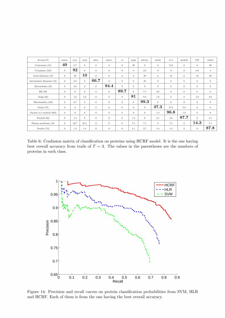
Accuracy% centro. cyto. actin inter. micro. er golgi mitoch. nuclei w/o nucleoli PM vesicle

Centrosome (15) 40 6.7 0 0 0 0 20 0 0 13.3 0 0 20

Cytoplasm (125) 0 92 0 0 0 0 0 3.2 0 0 0 0.8 4

Actin filaments (10) 0 20 10 0 0 0 0 30 0 10 0 10 20

Intermediate filaments (12) 0 8.3 0 66.7 0 0 0 25 0 0 0 0 0

Microtubules (18) 0 5.6 0 0 94.4 0 0 0 0 0 0 0 0

ER (39) 0 0 0 0 0 89.7 0 7.7 2.6 0 0 0 0

Golgi (63) 0 1.6 1.6 0 0 0 81 9.5 1.6 0 0 1.6 3.2

Mitochondria (148) 0 0.7 0 0 0 0 0 99.3 0 0 0 0 0

Nuclei (75) 0 0 0 0 0 0 0 0 37.3 57.3 5.3 0 0

Nucleus w/o nucleoli (284) 0 0 0 0 0 0 0 0 1.4 96.8 1.8 0 0

Nucleoli (65) 0 1.5 0 0 0 0 1.5 0 3.1 4.6 87.7 0 1.5

Plasma membrane (14) 0 35.7 21.4 0 0 0 7.1 7.1 0 7.1 0 14.3 7.1

Vesicles (74) 0 1.4 1.4 0 0 0 4.1 2.7 1.4 1.4 0 0 87.8

Table 6: Confusion matrix of classification on proteins using HCRF model. It is the one havingbest overall accuracy from trails of T = 3. The values in the parentheses are the numbers ofproteins in each class.

0 0.1 0.2 0.3 0.4 0.5 0.6 0.7 0.8 0.90.65

0.7

0.75

0.8

0.85

0.9

0.95

1

Recall

Pre

cisi

on

HCRFHLRSVM

Figure 14: Precision and recall curves on protein classification probabilities from SVM, HLRand HCRF. Each of them is from the one having the best overall accuracy.

28

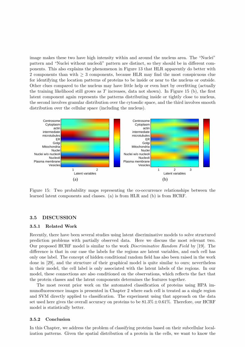
image makes these two have high intensity within and around the nucleus area. The “Nuclei”pattern and “Nuclei without nucleoli” pattern are distinct, so they should be in different com-ponents. This also explains the phenomenon in Figure 13 that HLR apparently do better with2 components than with ≥ 3 components, because HLR may find the most conspicuous cluefor identifying the location patterns of proteins to be inside or near to the nucleus or outside.Other clues compared to the nucleus may have little help or even hurt by overfitting (actuallythe training likelihood still grows as T increases, data not shown). In Figure 15 (b), the firstlatent component again represents the patterns distributing inside or tightly close to nucleus,the second involves granular distribution over the cytosolic space, and the third involves smoothdistribution over the cellular space (including the nucleus).

Latent variables

(a)

1 2

CentrosomeCytoplasm

actinintermediatemicrotubules

ERGolgi

MitochondriaNuclei

Nuclei w/o nucleoliNucleoli

Plasma membraneVesicles

Latent variables

(b)

1 2 3

CentrosomeCytoplasm

actinintermediatemicrotubules

ERGolgi

MitochondriaNuclei

Nuclei w/o nucleoliNucleoli

Plasma membraneVesicles

Figure 15: Two probability maps representing the co-occurrence relationships between thelearned latent components and classes. (a) is from HLR and (b) is from HCRF.

3.5 DISCUSSION

3.5.1 Related Work

Recently, there have been several studies using latent discriminative models to solve structuredprediction problems with partially observed data. Here we discuss the most relevant two.Our proposed HCRF model is similar to the work Discriminative Random Field by [19]. Thedifference is that in our case the labels for the regions are latent variables, and each cell hasonly one label. The concept of hidden conditional random field has also been raised in the workdone in [29], and the structure of their graphical model is quite similar to ours; neverthelessin their model, the cell label is only associated with the latent labels of the regions. In ourmodel, these connections are also conditioned on the observations, which reflects the fact thatthe protein classes and the latent components determines the features together.

The most recent prior work on the automated classification of proteins using HPA im-munofluorescence images is presented in Chapter 2 where each cell is treated as a single regionand SVM directly applied to classification. The experiment using that approach on the dataset used here gives the overall accuracy on proteins to be 81.3%± 0.61%. Therefore, our HCRFmodel is statistically better.

3.5.2 Conclusion

In this Chapter, we address the problem of classifying proteins based on their subcellular local-ization patterns. Given the spatial distribution of a protein in the cells, we want to know the

29

class of this protein.To solve this problem, we proposed two discriminative models that extend logistic regression

with latent variables. The first one, called the Hidden Logistic Regression (HLR), extendsregular logistic regression so that the features can depend on factors other than the class label.The HLR model addresses the issue that the same protein can be expressed differently atdifferent locations of the cell. The second model, called the Hidden Conditional Random Field(HCRF), further extends the HLR model by allowing the regions in the same cell to interactwith each other. HCRF is able to “guess” the component at a location based on informationfrom other regions, thus helping us better predict the class of the protein.

In both synthetic and real data experiments, we demonstrate that the proposed models areable to enhance classification performance. Particularly, on the HPA data set, HCRF achieved84.6% overall accuracy on proteins, which is best result up to now.

In the future, we plan to enhance the performance by using better features and devise moreaccurate learning algorithms. For example, we can incorporate richer dependencies betweencomponents. The features can also be transformed to take potential nonlinearity into consider-able. More efficient inference algorithm can be developed to allow for more complex interactionsbetween components. Moreover, because there are much larger amounts of images of proteinsthat can localize in more than one component in cell, we want to apply the models proposed inthis Chapter to classify more challenging protein subcellular location pattern complexes.

30

4 Overall Conclusion and Discussion

In this data analysis project, we completed two tasks which were both applied on HPA im-ages for computational experiments. Those HPA images were previously visually annotated totheir protein subcellular location patterns. One task (Chapter 2) was to build a first proteome-scale classification system using SVMs for automated recognition of protein subcellular locationpatterns and also to adopt unsupervised hierarchical clustering to complement. Moreover, onthe basis of the outputs from the two methods, we designed algorithms to identify potentialproteins which had high probabilities of being incorrectly annotated. Compared with the ran-dom sampling equivalence, we obtained up to 5.5-fold enrichment of such an identification ofmis-annotated proteins.

The second task (Chapter 3) tackled the classification problem making use of the region-based computer vision methods with discriminative modeling and latent variables. Given the re-gions, we were empowered with much more local information to model the spatial co-occurrencebetween protein distribution and cell components and between different cell components withinthe same cell. This strategy enabled us to improve the classification accuracy statistically sig-nificantly better than that from Chapter 2, and we got the highest overall accuracy around84.6%.

However, given the assumed limit in section 2.3.4 in Chapter 2, we still have space to improvefurther. Probably, we can design more sophisticated features on cell images to help us recognize,for example centrosome or plasma membrane patterns better, and also to design better solutionsfor heavily imbalanced dataset as we had in this project. Moreover, as shown in section 2.3.4in Chapter 2, we do not have good enough performance to recognize mixed pattern proteins.Local features may help, but we need to either optimize more on the algorithms in Chapter 3to be efficient enough to handle much more larger dataset, or to applied other local featureslike SURF [3]. We can also try to learn a local low dimensional embedding along a manifold inthe high dimension feature space to represent and “unmix” the continuous variations in mixedpattern between its individually constitutive patterns.

Furthermore, all the models and methods we discussed in this project are discriminativewhich basically can only answer the question of which protein pattern(s) is in a given image.To understand more of how such pattern(s) is generated, we should use generative models. Inthe past, there were many works [8] having been done in this field to build generative models onvesicular patterns [34,27] and filament microtubules patterns [30,31]. We can improve on thesemodels and use them to represent subcellular protein patterns in HPA, and then to identify theconditional dependences between them. Therefore, we shall eventually construct a complete,dynamic and quantitative network about subcellular location patterns in various human celllines, which will be significant and beneficial, i.e. to identify potential cancer biomarkers or tofacilitate drug screening and development.

31

Acknowledgments

We thank the Human Protein Atlas project team, especially Emma Lundberg, for providingthe high resolution fluorescence confocal microscopy images used in this study. We thank Drs.Murphy, Cohen and Kovacevic for the indispensable and insightful advisories. We thank Liangfor the collaboration. We also thank Dr. Gustavo K. Rohde, Dr. Justin Y. Newberg, Dr.Aabid Shariff, Dr. Tao Peng, Dr. Ting Zhao, Dr. Wei Wang, Cheng Chen and all Murphy Labmembers for their enthusiastic discussion and help.

References

[1] Ziv Bar-Joseph, David K. Gifford, and Tommi Jaakkola. Fast optimal leaf ordering forhierarchical clustering. In ISMB (Supplement of Bioinformatics), pages 22–29, 2001.

[2] L. Barbe, E. Lundberg, P. Oksvold, A. Stenius, E. Lewin, E. Bjorling, A. Asplund, F. Pon-ten, H. Brismar, M. Uhlen, and H. Andersson-Svahn. Toward a confocal subcellular atlasof the human proteome. Mol Cell Proteomics, 7:499–508, 2008.

[3] Herbert Bay, Andreas Ess, Tinne Tuytelaars, and Luc Van Gool. Speeded-up robust fea-tures (surf). Comput. Vis. Image Underst., 110(3):346–359, June 2008.

[4] Lisa Berglund, Erik Bjorling, Per Oksvold, Linn Fagerberg, Anna Asplund, Cristina Al-Khalili Szigyarto, Anja Persson, Jenny Ottosson, Henrik Wernerus, Peter Nilsson, EmmaLundberg, Asa Sivertsson, Sanjay Navani, Kenneth Wester, Caroline Kampf, Sophia Hober,Fredrik Ponten, and Mathias Uhlen. A genecentric human protein atlas for expressionprofiles based on antibodies. Molecular and Cellular Proteomics, 7(10):2019–2027, October2008.

[5] Christopher M. Bishop. Pattern Recognition and Machine Learning. Springer, 2006.

[6] Michael V. Boland and Robert F. Murphy. A neural network classifier capable of recognizingthe patterns of all major subcellular structures in fluorescence microscope images of helacells. Bioinformatics, 17(12):1213–1223, 2001.

[7] Leon Bottou. Online algorithms and stochastic approximations. In David Saad, editor,Online Learning and Neural Networks. Cambridge University Press, Cambridge, UK, 1998.

[8] T.E. Buck, J. Li, G.K. Rohde, and R.F. Murphy. Toward the virtual cell: Automatedapproaches to building models of subcellular organization “learnearned” from microscopyimages. BioEssays, 2012.

[9] Chih-Chung Chang and Chih-Jen Lin. Libsvm: A library for support vector machines.ACM Trans. Intell. Syst. Technol., 2(3):27:1–27:27, May 2011.

[10] Shann-Ching Chen, Ting Zhao, Geoffrey J. Gordon, and Robert F. Murphy. Automatedimage analysis of protein localization in budding yeast. Bioinformatics, 23(13):i66–i71,2007.

[11] Xiang Chen, Meel Velliste, and Robert F Murphy. Automated interpretation of subcellularpatterns in fluorescence microscope images for location proteomics. Cytometry Part A thejournal of the International Society for Analytical Cytology, 69(7):631–640, 2006.

[12] Luis Pedro Coelho, Tao Peng, and Robert F. Murphy. Quantifying the distribution ofprobes between subcellular locations using unsupervised pattern unmixing. Bioinformatics,26(12):i7–i12, 2010.

32

[13] RongEn Fan, KaiWei Chang, ChoJui Hsieh, XiangRui Wang, and ChihJen Lin. Liblinear:A library for large linear classification. 2008.

[14] Estelle Glory and Robert F Murphy. Automated subcellular location determination andhigh-throughput microscopy. Developmental Cell, 12(1):7–16, 2007.

[15] Nicholas Hamilton, Radosav Pantelic, Kelly Hanson, and Rohan Teasdale. Fast automatedcell phenotype image classification. BMC Bioinformatics, 8(1):110, 2007.

[16] Nicholas A. Hamilton and Rohan D. Teasdale. Visualizing and clustering high throughputsub-cellular localization imaging. BMC Bioinformatics, 9, 2008.

[17] Kai Huang, Meel Velliste, and Robert F. Murphy. Feature reduction for improved recog-nition of subcellular location patterns in fluorescence microscope images. pages 307–318,2003.

[18] Daphne Koller and Nir Friedman. Probabilistic Graphical Models: Principles and Tech-niques. The MIT Press, 2009.

[19] S. Kumar and M. Hebert. Discriminative fields for modeling spatial dependencies in naturalimages. In NIPS 16, 2004.

[20] John Lafferty, Andrew McCallum, and Fernando Pereira. Conditional random fields: Prob-abilistic models for segmenting and labeling sequence data. In ICML, 2001.

[21] Yu-Shi Lin, Yi-Hung Huang, Chung-Chih Lin, and Chun-Nan Hsu. Feature space trans-formation for semi-supervised learning for protein subcellular localization in fluorescencemicroscopy images. In Proceedings of the Sixth IEEE international conference on Sympo-sium on Biomedical Imaging: From Nano to Macro, ISBI’09, pages 414–417, Piscataway,NJ, USA, 2009. IEEE Press.

[22] David G. Lowe. Object recognition from local scale-invariant features. In Proceedings ofthe International Conference on Computer Vision-Volume 2 - Volume 2, ICCV ’99, pages1150–, Washington, DC, USA, 1999. IEEE Computer Society.

[23] J. Y. Newberg, J. Li, A. Rao, F. Ponten, M. Uhlen, E. Lundberg, and R. F. Murphy.Automated Analysis Of Human Protein Atlas Immunofluorescence Images. Proceedings ofthe 2009 IEEE International Symposium on Biomedical Imaging, pages 1023–1026, 2009.

[24] Justin Newberg and Robert F. Murphy. A framework for the automated analysis of sub-cellular patterns in human protein atlas images. J. Proteome Res, 2008.

[25] Jorge Nocedal and Stephen Wright. Numerical Optimization. Springer, 2000.

[26] Judea Pearl. Probabilistic Reasoning in Intelligent Systems: Networks of Plausible Infer-ence. Morgan Kaufmann, 1988.

[27] T. Peng and R.F. Murphy. Image-derived, three-dimensional generative models of cellularorganization. Cytometry A, 79(5):383–91, 2011.

[28] Tao Peng, Ghislain M. Bonamy, Estelle Glory-Afshar, Daniel R. Rines, Sumit K. Chanda,and Robert F. Murphy. Determining the distribution of probes between different subcellularlocations through automated unmixing of subcellular patterns. Proceedings of the NationalAcademy of Sciences of the United States of America, 107(7):2944–2949, February 2010.

[29] Ariadna Quattoni, Sybor Wang, Louis-Philippe Morency, Michael Collins, and Trevor Dar-rell. Hidden conditional random fields. IEEE Trans. PAMI, 29:1848 – 1853, 2007.

33

[30] A. Shariff, R.F. Murphy, and G.K. Rohde. A generative model of microtubule distributions,and indirect estimation of its parameters from fluorescence microscopy images. CytometryA, 2010.

[31] A. Shariff, R.F. Murphy, and G.K. Rohde. Automated estimation of microtubule modelparameters from 3-d live cell microscopy images. In Biomedical Imaging: From Nano toMacro, 2011 IEEE International Symposium on, pages 1330–1333. IEEE, 2011.

[32] Leo Breiman Statistics and Leo Breiman. Random forests. In Machine Learning, pages5–32, 2001.

[33] Mathias Uhlen, Erik Bjorling, Charlotta Agaton, Cristina Al-Khalili Szigyarto, BahramAmini, Elisabet Andersen, Ann-Catrin Andersson, Pia Angelidou, Anna Asplund, Caro-line Asplund, Lisa Berglund, Kristina Bergstrom, Harry Brumer, Dijana Cerjan, MaricaEkstrom, Adila Elobeid, Cecilia Eriksson, Linn Fagerberg, Ronny Falk, Jenny Fall, Mat-tias Forsberg, Marcus Gry Bjorklund, Kristoffer Gumbel, Asif Halimi, Inga Hallin, CarlHamsten, Marianne Hansson, My Hedhammar, Gorel Hercules, Caroline Kampf, KarinLarsson, Mats Lindskog, Wald Lodewyckx, Jan Lund, Joakim Lundeberg, Kristina Mag-nusson, Erik Malm, Peter Nilsson, Jenny Odling, Per Oksvold, Ingmarie Olsson, EmmaOster, Jenny Ottosson, Linda Paavilainen, Anja Persson, Rebecca Rimini, Johan Rockberg,Marcus Runeson, Asa Sivertsson, Anna Skollermo, Johanna Steen, Maria Stenvall, FredrikSterky, Sara Stromberg, Marten Sundberg, Hanna Tegel, Samuel Tourle, Eva Wahlund,Annelie Walden, Jinghong Wan, Henrik Wernerus, Joakim Westberg, Kenneth Wester,Ulla Wrethagen, Lan Lan Xu, Sophia Hober, and Fredrik Ponten. A human protein at-las for normal and cancer tissues based on antibody proteomics. Molecular and CellularProteomics, 4(12):1920–1932, December 2005.

[34] Ting Zhao and Robert F. Murphy. Automated learning of generative models for subcellularlocation: Building blocks for systems biology. Cytometry Part A, 71A(12):978–990, 2007.

34