Automated force controller for amplitude modulation atomic force microscopyAtsushi Miyagi and Simon Scheuring Citation: Review of Scientific Instruments 87, 053705 (2016); doi: 10.1063/1.4950777 View online: http://dx.doi.org/10.1063/1.4950777 View Table of Contents: http://scitation.aip.org/content/aip/journal/rsi/87/5?ver=pdfcov Published by the AIP Publishing Articles you may be interested in Stability, resolution, and ultra-low wear amplitude modulation atomic force microscopy of DNA: Smallamplitude small set-point imaging Appl. Phys. Lett. 103, 063702 (2013); 10.1063/1.4817906 High potential sensitivity in heterodyne amplitude-modulation Kelvin probe force microscopy Appl. Phys. Lett. 100, 223104 (2012); 10.1063/1.4723697 Analysis of the contrast mechanism in bimodal atomic force microscopy combining amplitude modulation andband excitation J. Appl. Phys. 111, 054909 (2012); 10.1063/1.3692393 Probe-surface interaction mapping in amplitude modulation atomic force microscopy by integrating amplitude-distance and amplitude-frequency curves Appl. Phys. Lett. 91, 023122 (2007); 10.1063/1.2756271 Dynamic proportional-integral-differential controller for high-speed atomic force microscopy Rev. Sci. Instrum. 77, 083704 (2006); 10.1063/1.2336113

Reuse of AIP Publishing content is subject to the terms at: https://publishing.aip.org/authors/rights-and-permissions. Download to IP: 139.124.66.250 On: Tue, 17 May

2016 15:37:27

REVIEW OF SCIENTIFIC INSTRUMENTS 87, 053705 (2016)

Automated force controller for amplitude modulation atomicforce microscopy

Atsushi Miyagia) and Simon Scheuringa)

U1006 INSERM, Université Aix-Marseille, Parc Scientifique et Technologique de Luminy,163 Avenue de Luminy, 13009 Marseille, France

(Received 1 April 2016; accepted 2 May 2016; published online 17 May 2016)

Atomic Force Microscopy (AFM) is widely used in physics, chemistry, and biology to analyze thetopography of a sample at nanometer resolution. Controlling precisely the force applied by the AFMtip to the sample is a prerequisite for faithful and reproducible imaging. In amplitude modulation(oscillating) mode AFM, the applied force depends on the free and the setpoint amplitudes ofthe cantilever oscillation. Therefore, for keeping the applied force constant, not only the setpointamplitude but also the free amplitude must be kept constant. While the AFM user defines the setpointamplitude, the free amplitude is typically subject to uncontrollable drift, and hence, unfortunately,the real applied force is permanently drifting during an experiment. This is particularly harmful inbiological sciences where increased force destroys the soft biological matter. Here, we have developeda strategy and an electronic circuit that analyzes permanently the free amplitude of oscillation andreadjusts the excitation to maintain the free amplitude constant. As a consequence, the real appliedforce is permanently and automatically controlled with picoNewton precision. With this circuitassociated to a high-speed AFM, we illustrate the power of the development through imaging overlong-duration and at various forces. The development is applicable for all AFMs and will widenthe applicability of AFM to a larger range of samples and to a larger range of (non-specialist)users. Furthermore, from controlled force imaging experiments, the interaction strength betweenbiomolecules can be analyzed. Published by AIP Publishing. [http://dx.doi.org/10.1063/1.4950777]

INTRODUCTION

Atomic force microscopy (AFM)1 is a powerful imagingtool for biological samples that allow imaging in aqueousenvironment with nanometer resolution. More recently, high-speed (HS-AFM) allows this performance, but additionallyprovides sub-second temporal resolution2,3 allowing for thefirst time the direct study of biomolecular processes at thesingle molecule level, such as myosin walking,4 membraneprotein diffusion,5 ATPase rotary motion,6 and membranedeformation.7 Amplitude modulation mode (also called: tapp-ing mode, oscillating mode, intermittent contact mode)8,9 isthe most popular AFM operation mode for biological samples,because of the quasi-elimination of lateral forces betweenAFM probe and sample. In typical amplitude modulationmode AFM, the cantilever is excited by acoustic waves toa free amplitude Afree, and the imaging amplitude setpointAset of the cantilever is kept constant by Z-movements of thesample stage driven by a feedback loop. The Z-movementof the sample stage, hence reflects the sample topography.The excitation efficiency, however, of how the acoustic wavesexcite the cantilever, changes permanently, probably becauseof the buffer evaporation and/or temperature changes and/orunknown factors. If the excitation efficiency rises, the canti-lever oscillation amplitude would increase, but the feedbackloop keeps it constant, resulting in a high applied force on the

a)Authors to whom correspondence should be addressed. Electronic ad-dresses: atsushi.miyagi@inserm.fr and simon.scheuring@inserm.fr. Tel.:++33-4-91828777. Fax: ++33-4-91828701.

sample, because the effective oscillation amplitude dampingis much higher. On the other hand, if the excitation efficiencydecreases, the cantilever oscillation amplitude would decreaseand approach the setpoint amplitude: as a result, the feedbackloop drives the tip out of sample contact. Several efforts havebeen reported to solve this problem: Cross correlation analysisbetween trace and retrace has been performed to detect force-dependent image quality changes and correct for those.10

More frequently, the amplitude of the second harmonic ofthe cantilever oscillation was used to detect free amplitudedrift.11 Alternatively, for contact mode imaging, the verticaland lateral vibrational noise of the cantilever has been usedto automatically modulate the force during imaging.12 Herewe present another, and as we believe more accurate, moresimple, and more general method (that is certainly bettersuited for soft biological samples), to compensate for freeamplitude drift: This method detects the “real free amplitude”several hundreds of times during a frame acquisition by takingadvantage of the fast scan axis “retrace scanning time.” Inour method, the Z-piezo retracts during every retrace scan torelease the tip from the sample surface. During this period, thefree amplitude is detected and compared to a free amplitudesetpoint, in order to generate a feedback signal to the excitationpiezo. In other words, there are always two feedback loopsoperating: the first, looking at and readjusting the actual freeamplitude Afree during every retrace scan line, and the second,more classical one looking at and readjusting the setpointamplitude Aset during image acquisition in the trace scan lines.The advantages of this method are multiple, as it that doesnot depend on tip conditions or sample properties. Even if

0034-6748/2016/87(5)/053705/6/$30.00 87, 053705-1 Published by AIP Publishing. Reuse of AIP Publishing content is subject to the terms at: https://publishing.aip.org/authors/rights-and-permissions. Download to IP: 139.124.66.250 On: Tue, 17 May

2016 15:37:27

053705-2 A. Miyagi and S. Scheuring Rev. Sci. Instrum. 87, 053705 (2016)

an organic molecule is attached to the tip, and whatever bethe sample elasticity from a very soft biological object to the“infinitely” hard mica substrate, this method is unaffected andcontinues adjusting the real applied force with accuracy.

RESULTS

The principle of the automated free amplitudeand force controller

In amplitude modulation mode AFM, the cantileveroscillation setpoint amplitude Aset is kept constant by feedbackon the Z-piezo extension. While this is the classical principle ofAFM operation, the permanent maintenance of the cantileveroscillation amplitude to Aset actually inhibits the operator (andthe machine) from knowing what the actual free amplitudeAfree is. This is regrettable, yet, we can take advantage ofthe retrace scan time (when the tip moves backwards, scanthat is not used for image formation) and retract the samplesurface from the AFM probe during this period and detect theactual free amplitude Afree. This is achieved here by addingan electronic circuit to a high-speed AFM (HS-AFM); thedevelopment can however be implemented into any AFMsystem.

During image acquisition a triangular voltage signal issent to the X-piezo (Figure 1(a)), which leads to forth andback X-scanning, i.e., the so-called fast scan axis, of the imageacquisition. Every time, the X-scanning “turns around”, i.e.,the X-piezo voltage changes from increasing to decreasingvalues and the relative scan motion changes from left-rightto right-left, a trigger signal is generated: When the force-controller circuit receives this trigger signal, it sends a “mock”signal to the PID Z-feedback controller to adjust the imagingsetpoint amplitude Aset to a high “mock” value Amock, whichis actually larger than Afree. As a consequence the Z-piezoimmediately retracts to result in complete separation of theAFM tip from the sample surface (Figure 1(b)). It is duringthis retract period when the cantilever swings freely out ofcontact (Figure 1(c)) that a short amplitude analysis windowopens (Figure 1(c), red bar) and the actual free amplitudeAfree is detected. Immediately after free amplitude detection,the circuit sets the imaging amplitude setpoint back to itsoriginal value Aset, smaller than Afree, and the AFM feedbackwill automatically drive the probe back into contact with thesample surface, before starting the next trace imaging fastscan line. Importantly, as a consequence of the performedAfree detection, the circuit adjusts the excitation power that issent to the cantilever excitation piezo to keep Afree constant.

Inspection of the retrace “image” shows a vertical brightline on the right edge that corresponds to the lift-off regimewhen Afree is detected (Figure 1(d)), i.e., the peak in the“tip-sample distance” trace (compare Figure 1(b)). In thepresented example, the imaging condition are the following:free amplitude Afree is set to 1 nm, the imaging amplitudesetpoint Aset is set to 90% of Afree, i.e., 0.92 nm, the framesize is 200 × 200 pixels, and the scan speed is 1 frame/s. The“mock” set point amplitude Amock was set to 110% of Afreeand sent during 100 µs, leading to complete separation of tipand sample, here about 4.5 nm (Figure 1(d); section profile).

FIG. 1. Scan signals during free amplitude Afree detection. (a) One cycle ofthe X-piezo voltage signal. The X-piezo represents the fast-scan axis. Thelinear voltage increases from 0 V to 3 V is the “trace” and from 3 V to 0 Vthe “retrace” scan line. In our HS-AFM system, this cycle is completed in alittle less than 5 ms. (b) Tip-sample distance: A mock signal at the beginningof the “retrace” scan line (blue dashed line) leads to retraction of the tip fromthe surface. (c) Cantilever oscillation amplitude: During surface scanning, theamplitude is kept to about 0.92 nm by feedback control. During tip retraction,the amplitude reaches Afree that is detected during a time window (red bar) of10 oscillation cycles. (d) HS-AFM retrace “image” (top) and section profile(bottom) along the dashed line in the image. The tip-retraction period for Afreeanalysis is visible on the right “image” edge and is represented by a 4.5 nmpeak in the section profile.

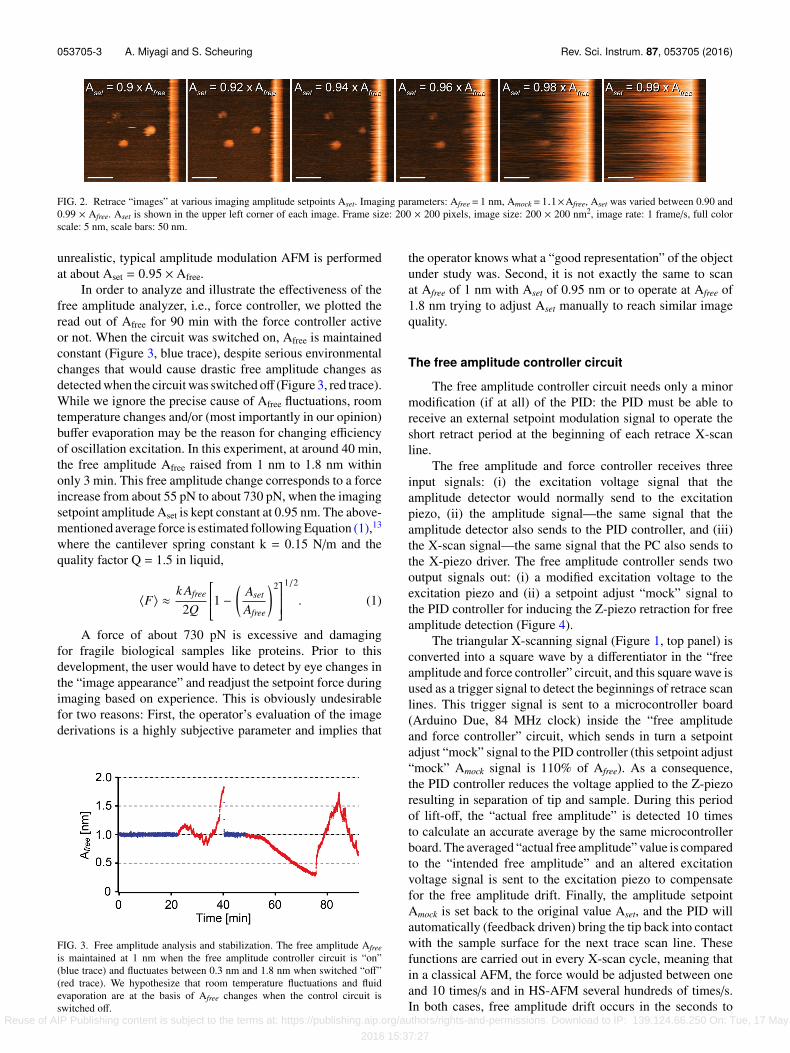
4.5 nm is far enough from the surface to detect accuratelythe actual free amplitude (that is around 1 nm) and closeenough to the surface to reach contact before beginning ofthe next trace imaging scan line. The separation distance canbe adjusted by changing Amock and the duration during whichAmock is sent to the PID. A larger and/or longer Amock signalwould lead to a larger separation between tip and sample. Thetime it takes for the PID to drive the tip back into contact fromAmock = 1.1 × Afree to Aset depends on the value of Aset. To testthis, we defined Aset to 90%, 92%, 94%, 96%, 98% or 99% ofAfree (Figure 2). At Aset of 98%, “parachuting” (period of timeduring which the tip and the sample are separated while thefeedback drives them back into contact) is clearly visible butthe tip gets readily back into contact to the sample surfacebefore the next trace scan. Only when Aset = 0.99 × Afree,the “parachuting” might eventually reach the next trace scanline (Figure 2, rightmost panel); such conditions are however

Reuse of AIP Publishing content is subject to the terms at: https://publishing.aip.org/authors/rights-and-permissions. Download to IP: 139.124.66.250 On: Tue, 17 May

2016 15:37:27

053705-3 A. Miyagi and S. Scheuring Rev. Sci. Instrum. 87, 053705 (2016)

FIG. 2. Retrace “images” at various imaging amplitude setpoints Aset. Imaging parameters: Afree= 1 nm, Amock= 1.1×Afree, Aset was varied between 0.90 and0.99 × Afree. Aset is shown in the upper left corner of each image. Frame size: 200 × 200 pixels, image size: 200 × 200 nm2, image rate: 1 frame/s, full colorscale: 5 nm, scale bars: 50 nm.

unrealistic, typical amplitude modulation AFM is performedat about Aset = 0.95 × Afree.

In order to analyze and illustrate the effectiveness of thefree amplitude analyzer, i.e., force controller, we plotted theread out of Afree for 90 min with the force controller activeor not. When the circuit was switched on, Afree is maintainedconstant (Figure 3, blue trace), despite serious environmentalchanges that would cause drastic free amplitude changes asdetected when the circuit was switched off (Figure 3, red trace).While we ignore the precise cause of Afree fluctuations, roomtemperature changes and/or (most importantly in our opinion)buffer evaporation may be the reason for changing efficiencyof oscillation excitation. In this experiment, at around 40 min,the free amplitude Afree raised from 1 nm to 1.8 nm withinonly 3 min. This free amplitude change corresponds to a forceincrease from about 55 pN to about 730 pN, when the imagingsetpoint amplitude Aset is kept constant at 0.95 nm. The above-mentioned average force is estimated following Equation (1),13

where the cantilever spring constant k = 0.15 N/m and thequality factor Q = 1.5 in liquid,

⟨F⟩ ≈ k Afree

2Q

1 −

(Aset

Afree

)2

1/2

. (1)

A force of about 730 pN is excessive and damagingfor fragile biological samples like proteins. Prior to thisdevelopment, the user would have to detect by eye changes inthe “image appearance” and readjust the setpoint force duringimaging based on experience. This is obviously undesirablefor two reasons: First, the operator’s evaluation of the imagederivations is a highly subjective parameter and implies that

FIG. 3. Free amplitude analysis and stabilization. The free amplitude Afreeis maintained at 1 nm when the free amplitude controller circuit is “on”(blue trace) and fluctuates between 0.3 nm and 1.8 nm when switched “off”(red trace). We hypothesize that room temperature fluctuations and fluidevaporation are at the basis of Afree changes when the control circuit isswitched off.

the operator knows what a “good representation” of the objectunder study was. Second, it is not exactly the same to scanat Afree of 1 nm with Aset of 0.95 nm or to operate at Afree of1.8 nm trying to adjust Aset manually to reach similar imagequality.

The free amplitude controller circuit

The free amplitude controller circuit needs only a minormodification (if at all) of the PID: the PID must be able toreceive an external setpoint modulation signal to operate theshort retract period at the beginning of each retrace X-scanline.

The free amplitude and force controller receives threeinput signals: (i) the excitation voltage signal that theamplitude detector would normally send to the excitationpiezo, (ii) the amplitude signal—the same signal that theamplitude detector also sends to the PID controller, and (iii)the X-scan signal—the same signal that the PC also sends tothe X-piezo driver. The free amplitude controller sends twooutput signals out: (i) a modified excitation voltage to theexcitation piezo and (ii) a setpoint adjust “mock” signal tothe PID controller for inducing the Z-piezo retraction for freeamplitude detection (Figure 4).

The triangular X-scanning signal (Figure 1, top panel) isconverted into a square wave by a differentiator in the “freeamplitude and force controller” circuit, and this square wave isused as a trigger signal to detect the beginnings of retrace scanlines. This trigger signal is sent to a microcontroller board(Arduino Due, 84 MHz clock) inside the “free amplitudeand force controller” circuit, which sends in turn a setpointadjust “mock” signal to the PID controller (this setpoint adjust“mock” Amock signal is 110% of Afree). As a consequence,the PID controller reduces the voltage applied to the Z-piezoresulting in separation of tip and sample. During this periodof lift-off, the “actual free amplitude” is detected 10 timesto calculate an accurate average by the same microcontrollerboard. The averaged “actual free amplitude” value is comparedto the “intended free amplitude” and an altered excitationvoltage signal is sent to the excitation piezo to compensatefor the free amplitude drift. Finally, the amplitude setpointAmock is set back to the original value Aset, and the PID willautomatically (feedback driven) bring the tip back into contactwith the sample surface for the next trace scan line. Thesefunctions are carried out in every X-scan cycle, meaning thatin a classical AFM, the force would be adjusted between oneand 10 times/s and in HS-AFM several hundreds of times/s.In both cases, free amplitude drift occurs in the seconds to

Reuse of AIP Publishing content is subject to the terms at: https://publishing.aip.org/authors/rights-and-permissions. Download to IP: 139.124.66.250 On: Tue, 17 May

2016 15:37:27

053705-4 A. Miyagi and S. Scheuring Rev. Sci. Instrum. 87, 053705 (2016)

FIG. 4. Schematic of the “free amplitude and force controller” circuit withinan amplitude modulation AFM. Electronic devices are represented by rectan-gular boxes and signals by arrows. The “free amplitude and force controller”circuit is shown in red and the “novel” signals by red arrows.

minutes range, and therefore this development can be appliedand will be effective to any type of amplitude modulationAFM.

Automated imaging at various well-controlled forces

In addition to free amplitude Afree control for long-duration force-controlled imaging stabilization, the circuit canequally be used to adjust the imaging setpoint amplitude Aset

(together with Afree), even in subregions of each image. Toillustrate this function, the chaperonin GroEL double ringswere imaged head-on adsorbed onto the mica support at fourdifferent well-defined imaging forces (Figure 5). Afree was setto 1 nm. During the first 50 lines (bottom part of the image), the

imaging amplitude setpoint is 97% of the free amplitude, thesecond 50 lines were imaged with 95%, the third 50 lines with93% and the last 50 lines with 91% of Afree (Figure 5(a)). Usingfree amplitude control, Afree was set to 1 nm and kept constantat this value, while Aset was modulated to the above-mentionedfractions of Afree every 50 lines. The estimated average appliedloading forces are 33 pN, 55 pN, 76 pN, and 97 pN for eachsection, as estimated following Equation (1).

The capacity of imaging at various forces in one imagehas itself two advantages: first, it allows to test for idealimaging conditions within a single frame and hence avoidlong force adjustment experiments that risk to contaminatethe tip. And second, it allows us to analyze the effect of forceon the biological sample and derive biophysical parametersfrom it. Here, GroEL14 were images on mica at four differentforces. GroEL is a barrel-shaped chaperonin of about 14 nmin diameter and about 16 nm in height, consisting of twostacked rings (14 nm in diameter and 8 nm in height).14

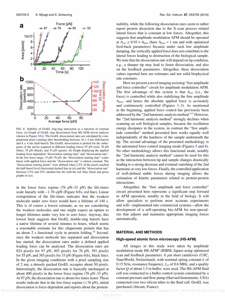
GroEL is an interesting sample for our purpose: first, becausethe two rings are only weakly bound and can be dissociatedas function of the applied force15,16 and hence allows toevaluate the sensitivity of the force controller and second,because the result allowed us to illustrate how interactionkinetics between biomolecules can be estimated from suchexperiments. The force-dependent dissociation of the GroELupper rings was determined by measuring the areas of about16 nm in height (full GroEL barrel, double ring) and theareas of about 8 nm in height (only lower GroEL half-barrel, single ring) on the mica surface (Figure 5(b)). Giventhat GroEL is scanned at four different forces, nominally33 pN, 55 pN, 76 pN, and 97 pN, respectively, withineach image frame, the beginning instant and the rate ofGroEL upper ring dissociation can be plotted as a functionof applied force (Figure 6(a)). These four dissociation curvesat different forces allow us to draw a first most importantconclusion: The “free amplitude and force controller” circuitworks properly. With increased forces, dissociation occursmore rapidly (Figures 5(b) and 6(a)). Furthermore, from thesedissociation graphs, two major parameters can be extracted:First, the dissociation starting points are 2 s for 97 pN, 6 sfor 76 pN, 46 s for 55 pN, and 82 s for 33 pN, respectively.The beginning of the dissociation represents the life-time ofthe weakest molecule under a given force load. Interestingly,

FIG. 5. Imaging at various well-controlled imaging forces. (a) Representation of the four imaging forces, i.e., setpoint amplitudes Aset expressed as fractionsof Afree. Aset was set to 97%, 95%, 93%, 91% of Afree corresponding to average loading forces of nominally 33 pN, 55 pN, 76 pN, and 97 pN, respectively.Afree was set to 1 nm and kept constant at this value using the free amplitude control circuit. Imaging parameters: image size: 200 × 200 pixels, frame size: 400× 400 nm2, imaging speed: 2 s/frame, cantilever spring constant k : 0.15 N/m, cantilever Q factor: 1.5. (b) Images of a movie acquired at four different loadingforces, i.e., amplitude setpoints as illustrated in (a), every 50 scan lines (indicated by the dashed lines). Scale bars: 100 nm. The upper ring of the GroEL barreldissociates progressively with time and as function of the applied force.

Reuse of AIP Publishing content is subject to the terms at: https://publishing.aip.org/authors/rights-and-permissions. Download to IP: 139.124.66.250 On: Tue, 17 May

2016 15:37:27

053705-5 A. Miyagi and S. Scheuring Rev. Sci. Instrum. 87, 053705 (2016)

FIG. 6. Stability of GroEL ring-ring interaction as a function of externalforce. (a) Graph of GroEL ring dissociation from HS-AFM movie analysis(shown in Figure 5(b)). The GroEL dissociation rates are calculated by com-putational pixel counting after thresholding between 16 ± 4 nm (full-barrel)and 8 ± 4 nm (half-barrel) The GroEL dissociation is plotted for the subre-gions of the movie acquired at different loading forces 97 pN (red), 76 pN(blue), 55 pN (black), and 33 pN (green). (b) Graph displaying the appliedloading force dependent “dissociation starting time” and “dissociation rate”.In the low-force range, 33 pN–76 pN, the “dissociation starting time” scaleslinear with applied force and the “dissociation rate” is almost constant. The“dissociation starting points” were defined when 2.5% of the pixels reachedthe half-barrel level (horizontal dashed line in (a)) and the “dissociation rate”between 2.5% and 25% (dashed line fits with the red, blue, black and greengraphs in (a)).

in the lower force regime (76 pN–33 pN) the life-timesscale linearly with −1.76 s/pN (Figure 6(b), red line). Linearextrapolation of the life-times indicates that the weakestmolecule under zero force would have a lifetime of 140 s.This is of course a lowest estimate, as we are consideringthe weakest molecules and one might expect an upturn tolonger lifetimes under very low to zero force. Anyway, thislowest limit suggests that GroEL double-ring barrels havea native lifetime of several minutes to hours, which seemsa reasonable estimate for this chaperonin protein that hasan about 2 s functional cycle in protein folding.16 Second,once the weakest molecule has separated and dissociationhas started, the dissociation rates under a defined appliedloading force can be analyzed. The dissociation rates are824 pixel/s for 97 pN, 403 pixel/s for 76 pN, 391 pixel/sfor 55 pN, and 385 pixel/s for 33 pN (Figure 6(b), black line).In the given imaging conditions with a pixel sampling sizeof 2 nm, a densely packed GroEL occupies about 50 pixels.Interestingly, the dissociation rate is basically unchanged atabout 400 pixel/s in the lower force regime (76 pN–33 pN).At 97 pN, the dissociation rate is about two times faster. Theseresults indicate that in the low-force regime (<76 pN), initialdissociation is force-dependent and reports about the protein-

stability, while the following dissociation rates seem to ratherreport protein dissection due to the X-scan process relatedlateral forces that is constant at low forces. Altogether, thissuggests that amplitude modulation AFM should be operatedat Aset ≥ 0.93 × Afree (here Afree = 1 nm and with optimizedfeed-back parameters) because under such low amplitudedamping, the vertically applied force does not contribute to thelateral forces leading to destruction of the biological sample.We note that the dissociation rate will depend on tip condition,e.g., a sharper tip may lead to faster dissociation, and alsoon the feedback parameters. Altogether, these dissociationvalues reported here are estimates and not solid biophysicalrate constants.

Here we present a novel imaging assisting “free amplitudeand force controller” circuit for amplitude modulation AFM.The first advantage of this system is that Aset (i.e., theforce) is controlled while also stabilizing the free amplitudeAfree, and hence the absolute applied force is accuratelyand continuously controlled (Figures 1–3). As mentionedin the beginning, applied force control has previously beenaddressed by the “2nd harmonic analysis method.”11 However,the “2nd harmonic analysis method” strongly declines whenscanning on soft biological samples, because the oscillationenergy dissipates in the system, in contrast the “free ampli-tude controller” method presented here works equally wellindependently of the hardness of the sample underneath thetip. The second advantage of the presented methodology isthe automated force control imaging mode (Figures 5 and 6).No other methodology allows this functional mode, notablythe “2nd harmonic analysis method” cannot be used for thisas the interaction between tip and sample changes drasticallyleading to a strong decrease and eventual vanishing of the 2ndharmonic at very low forces. Finally, the controlled applicationof well-defined stable forces during imaging allows theestimation of kinetic parameters related to protein-proteininteractions.

Altogether, the “free amplitude and force controller”circuit presented here represents a significant step forwardin AFM operation, notably in the field of biology. It willallow specialists to perform more accurate experimentsand will—implemented into commercial systems—allow thedevelopment of a self-operating bio-AFM for non-special-ists that adjusts and maintains appropriate imaging forcesautomatically.

MATERIAL AND METHODS

High-speed atomic force microscopy (HS-AFM)

All images in this study were taken by amplitudemodulation mode HS-AFM6 (RIBM, Japan) using optimizedscan and feedback parameters. 8 µm short cantilevers (USC,NanoWorld, Switzerland), with nominal spring constant k of0.15 N/m, resonance frequency f (r) of 0.6 MHz, and a qualityfactor Q of about 1.5 in buffer, were used. The HS-AFM fluidcell was connected to a buffer control system constituted by aconstant pressure and flow pump (Harvard Instruments, USA)connected over two silicon tubes to the fluid cell. GroEL waspurchased (Abcam, France).

Reuse of AIP Publishing content is subject to the terms at: https://publishing.aip.org/authors/rights-and-permissions. Download to IP: 139.124.66.250 On: Tue, 17 May

2016 15:37:27

053705-6 A. Miyagi and S. Scheuring Rev. Sci. Instrum. 87, 053705 (2016)

Sample preparation

GroEL (Abcam, France) was diluted in a buffer solution(20 mM Tris, pH 7.3, 30 mM KCl, 10 mM MgCl2) to afinal concentration of 100 nM. 1 µl of GroEL was put ontofreshly cleaved mica for 1 h at room temperature in a humidchamber. Then non-adsorbed GroEL was rinsed off with thesame buffer.

Data analysis

HS-AFM images were analyzed by using the particlesanalysis plugin in imageJ using a threshold between the heightof the GroEL double-ring barrel (16 nm) and the single-ring(8 nm). The lifetime of the beginning of dissociating underforce, i.e., the dissociation of the upper GroEL ring of theweakest molecule under vertical force, was evaluated when2.5% (dashed horizontal line in Figure 6(a)) of the imagedarea (the area of a specific force regime in Figure 5(b))displayed pixel values lower than threshold, and the followingdissociation rate, i.e., the progression of dissociation of theupper GroEL ring due to lateral force, was evaluated in theregime of 2.5%–25% of the total area occupied by pixel valueslower than threshold.

ACKNOWLEDGMENTS

This work was funded by a European Research Council(ERC) Consolidator Grant (No. 310080).

1G. Binnig, C. F. Quate, and C. Gerber, Phys. Rev. Lett. 56, 930 (1986).2T. Ando, N. Kodera, E. Takai, D. Maruyama, K. Saito, and A. Toda, Proc.Natl. Acad. Sci. U. S. A. 98, 12468 (2001).

3T. Ando, T. Uchihashi, and S. Scheuring, Chem. Rev. 114, 3120 (2014).4N. Kodera, D. Yamamoto, R. Ishikawa, and T. Ando, Nature 468, 72 (2010).5I. Casuso, J. Khao, M. Chami, P. Paul-Gilloteaux, M. Husain, J. P. Duneau,H. Stahlberg, J. N. Sturgis, and S. Scheuring, Nat. Nanotechnol. 7, 525(2012).

6T. Uchihashi, R. Iino, T. Ando, and H. Noji, Science 333, 755 (2011).7N. Chiaruttini, L. Redondo-Morata, A. Colom, F. Humbert, M. Lenz, S.Scheuring, and A. Roux, Cell 163, 866 (2015).

8P. K. Hansma, J. P. Cleveland, M. Radmacher, D. A. Walters, P. E. Hillner,M. Bezanilla, M. Fritz, D. Vie, H. G. Hansma, C. B. Prater, J. Massie, L.Fukunaga, J. Gurley, and V. Elings, Appl. Phys. Lett. 64, 1738 (1994).

9R. García and A. San Paulo, Phys. Rev. B 60, 4961 (1999).10J. H. Kindt, J. B. Thompson, M. B. Viani, and P. K. Hansma, Rev. Sci.

Instrum. 73, 2305 (2002).11N. Kodera, M. Sakashita, and T. Ando, Rev. Sci. Instrum. 77, 083704 (2006).12I. Casuso and S. Scheuring, Nanotechnology 21, 035104 (2010).13R. García, Amplitude Modulation Atomic Force Microscopy (Wiley-VCH

Verlag GmbH & Co. KGaA, 2010).14F. U. Hartl, Nature 381, 571 (1996).15J. Mou, S. Sheng, R. Ho, and Z. Shao, Biophys. J. 71, 2213 (1996).16F. J. Corrales and A. R. Fersht, Proc. Natl. Acad. Sci. U. S. A. 92, 5326

(1995).

Reuse of AIP Publishing content is subject to the terms at: https://publishing.aip.org/authors/rights-and-permissions. Download to IP: 139.124.66.250 On: Tue, 17 May

2016 15:37:27