automated animal coloration quantification in digital ... · automated animal coloration...

Automated Animal Coloration Quantification in Digital Images using Dominant Colors

and Skin Classification.

by

Tejas Borkar

A Thesis Presented in Partial Fulfillment

of the Requirements for the Degree

Master of Science

Approved November 2013 by the

Graduate Supervisory Committee:

Lina Karam, Chair

Baoxin Li

Kevin McGraw

ARIZONA STATE UNIVERSITY

December 2013

i

ABSTRACT

The origin and function of color in animals has been a subject of great interest for

taxonomists and ecologists in recent years. Coloration in animals is useful for many

important functions like species identification, camouflage and understanding

evolutionary relationships. Quantitative measurements of color signal and patch size in

mammals, birds and reptiles, to name a few are strong indicators of sexual selection cues

and individual health. These measurements provide valuable insights into the impact of

environmental conditions on habitat and breeding of mammals, birds and reptiles. Recent

advances in the area of digital cameras and sensors have led to a significant increase in

the use of digital photography as a means of color quantification in animals. Although a

significant amount of research has been conducted on ways to standardize image

acquisition conditions and calibrate cameras for use in animal color quantification, almost

no work has been done on designing automated methods for animal color quantification.

This thesis presents a novel perceptual-based framework for the automated

extraction and quantification of animal coloration from digital images with slowly

varying (almost homogenous) background colors. This implemented framework uses a

combination of several techniques including color space quantization using a few

dominant colors, foreground-background identification, Bayesian classification and

mixture Gaussian modelling of conditional densities, edge-enhanced model-based

classification and Saturation-Brightness quantization to extract the colored patch. This

approach assumes no prior information about the color of either the subject or the

background and also the position of the subject in the image. The performance of the

proposed method is evaluated for the plumage color of the wild house finches.

ii

Segmentation results obtained using the implemented framework are compared with

manually scored results to illustrate the performance of this system. The segmentation

results show a high correlation with manually scored images. This novel framework also

eliminates common problems in manual scoring of digital images such as low

repeatability and inter-observer error.

iii

To my loving parents and brother Varun.

iv

ACKNOWLEDGMENTS

I would like to acknowledge the strong guidance and invaluable support of my thesis

advisor Dr. Lina J. Karam in helping me bring this thesis to fruition. I would like to thank

Dr. Baoxin Li and Dr. Kevin J. McGraw for agreeing to serve on my committee and

providing valuable suggestions. I would also like to thank Dr. Mathieu Giraudeau for his

time and support towards this work.

I would like to acknowledge the support provided by all the members of the Image,

Video and Usability (IVU) lab. I would specially like to acknowledge the extremely

valuable assistance provided by my fellow lab mates Charan Prakash, Vinay Kashyap

and Bashar Haddad. I would like to make a special mention of my close friends Shreyas,

Pratik, Rohan and Manjiri for their constant support and encouragement throughout my

journey. Last but definitely not the least, I would like to express my utmost gratitude to

my parents and elder brother Varun for their strong love and support all throughout my

journey.

v

TABLE OF CONTENTS

Page

LIST OF TABLES ................................................................................................................. vii

LIST OF FIGURES .............................................................................................................. viii

CHAPTER

1 INTRODUCTION ..............................................................................................................1

1.1 Motivation .................................................................................................................. 1

1.2 Contributions .............................................................................................................. 4

1.3 Thesis Organization ..............................................................................................5

2 BACKGROUND ................................................................................................................7

2.1 Color Spaces .............................................................................................................. 7

2.1.1 CIE (R, G, B) color space .............................................................................. 8

2.1.2 CIE (L*, a*, b*) color space (also known as CIELAB) ...........................11

2.1.3 (H, S, V) color space ...............................................................................12

2.2 Gaussian Mixture Model Estimation using Expectation-Maximization ............16

2.3 Bayesian Decision Theory ..................................................................................18

3 RELATED WORK ..................................................................................................... 21

3.1 Manual Software Methods ..................................................................................21

3.2 Automated Quantification Method .....................................................................23

4 IMPLEMENTED AUTOMATED COLOR QUANTIFICATION SYSTEM ............. 25

4.1 Overview of the Proposed System ......................................................................25

4.2 Foreground Extraction and Background Removal using Dominant Colors .......29

4.2.1 Dominant color extraction in images ......................................................30

vi

CHAPTER Page

4.2.2 Foreground extraction using k-means clustering ....................................34

4.3 Skin/Non Skin Region Classification...................................................................36

4.4 Edge-Enhanced Model-Based Classification for Outlier Pixel Removal ............40

4.5 Perceptual-based Saturation-Value Quantization ................................................44

4.6 MATLAB-based Software Implementation. ........................................................47

5 RESULTS .................................................................................................................. 50

5.1 Data Set Description ............................................................................................50

5.2 Manual Results Generation .................................................................................53

5.3 Inter-photo and Intra Photo Repeatability ...........................................................54

5.4 Correlation Analysis of the Proposed Framework ...............................................60

6 CONCLUSION .......................................................................................................... 72

6.1 Contributions .......................................................................................................72

6.2 Future Research Directions .................................................................................73

REFERENCES ................................................................................................................. 75

APPENDIX

A ANOVA TABLES AND VARIANCE COMPONENT TABLES ............................ 80

vii

LIST OF TABLES

Table Page

1. Inter-photo Repeatability of software and hand scored results for Dataset 1. ............ 58

2. Inter-photo Repeatability of software and hand scored results for Dataset 2. ............ 58

3. Intra-photo Repeatability of software and hand scored results for Dataset 1. ............ 59

4. Intra-photo Repeatability of software and hand scored results for Dataset 2. ............ 59

5. Linear correlation of proposed method with user scored results for Dataset 1. .......... 61

6. Linear correlation of proposed method with user scored results for Dataset 2. ......... 61

viii

LIST OF FIGURES

Figure Page

1. RGB color cube. ............................................................................................................ 9

2. HSV model representation using cylindrical co-ordinates. ......................................... 14

3. Projection of tilted RGB cube on a plane.....................................................................14

4. Original image with the color strip present..................................................................26

5. Binary image showing the detected color square in white, for color strip removal. .. 26

6. Image obtained after removing the color strip from the image. ................................. 27

7. Block diagram of the proposed framework. ............................................................... 28

8. Original image containing multiple colors. ................................................................ 32

9. Image Segmentation result using 14 dominant colors. .............................................. 32

10. Segmentation result using 8 dominant colors. ........................................................... 33

11. Segmentation result using 5 dominant colors. ........................................................... 33

12. Input image. ............................................................................................................... 35

13. Foreground-background class abstraction for the image shown in Fig. 12; foreground

region shown in white. ................................................................................................ 35

14. Sample images from the skin dataset used to estimate the skin condition.................38

15. Binary edge map. ....................................................................................................... 43

16. Hand region mask. ..................................................................................................... 43

17. Final generated ROI mask ......................................................................................... 43

18. Plot of Value versus Saturation for a single hue (Hue = 6º).......................................45

19. Quantization decision boundary overlay on Value versus Saturation plot.................45

ix

Figure Page

20. Binary mask generated using perceptual-based Saturation-Value quantization. ........ 46

21. Outline of final extracted ROI overlayed on original image ...................................... 49

22. User interface for MATLAB-based implementation of proposed method. ................ 49

23. Example images from the rump dataset (Dataset 1). .................................................. 51

24. Example images from the breast dataset (Dataset 2). ................................................. 52

25. Correlation scatter plots for measured hue of Dataset 1. (a) Relation between

proposed method and user 1. (b) Relation between proposed method and user 2. (c)

Relation between proposed method and user 3. .......................................................... 62

26. Correlation scatter plots for measured saturation of Dataset 1. (a) Relation between



27. Correlation scatter plots for measured value of Dataset 1. (a) Relation between



28. Correlation scatter plots for measured patch size of Dataset 1. (a) Relation between



29. Correlation scatter plots for measured hue of Dataset 2. (a) Relation between



x

Figure Page

30. Correlation scatter plots for measured saturation of Dataset 2. (a) Relation between



31. Correlation scatter plots for measured value of Dataset 2. (a) Relation between



32. Correlation scatter plots for measured patch size of Dataset 2. (a) Relation between



33. Performance relationship between results generated using proposed scheme and user

scored results for dataset 1 and dataset 2. ................................................................... 70

1

CHAPTER 1

INTRODUCTION

This chapter presents the motivations behind the work in this thesis and briefly

summarizes the contributions and organization of the thesis.

1.1 Motivation

The origin and function of coloration in animals has been a topic of immense interest and

research for taxonomists and ecologists [1], [2]. Humans have always been intrigued by

the bright color patterns observed in various animal species such as the bright plumage

colors in most birds or the various multicolor patterns on the wings of butterflies, which

is unlike the murky and earthen colors observed in most mammals. This coloration in

animals serves many important functions like camouflage, mate selection during

breeding, sexual dimorphism and species identification, to name a few [1].

The coloration in animals is a result of a number of different factors. For example,

the earth tone, gray, black and brown color observed in most mammals is produced due

to a pigment called melanin [3], while the bright plumage coloration observed in birds is

the result of a combination of melanin based color, carotenoid pigment based color and

structural color due to feathers. Understanding the origin of these color signals and their

quantification helps researchers in getting a better understanding of the environmental

conditions that affect the habitat and breeding of these animal species. For example,

melanin and carotenoid pigments are the most prominent pigments responsible for

coloration in birds. Melanin is responsible for the black, gray, brown and earth tone

colors present in most birds [3]. Since melanin is produced within the body, melanin

based color variation is not strongly correlated to environmental changes [1]. Carotenoid

2

pigments however, are not produced within the bird’s body and are actually acquired

through the bird’s diet. Carotenoid pigments are responsible for the bright red, orange

and yellow plumage colors observed in many birds [4]. Since the carotenoid pigments are

derived from diets, quantitative measurements of these bright plumage colors provide

great insights into the quality of diet, habitat and individual health of the these birds.

Such measurements are also believed to be strong indicators of sexual selection cues [5].

Since environmental conditions and dietary changes affect the carotenoid pigment

concentrations in birds, plumage coloration measurement in birds is an important trait for

ecologists, taxonomists, conservationists and sustainability scientists. These

measurements have been also used for subspecies identification [6].

Animal color quantification refers to the approach of characterizing the coloration

observed in individual animals using colorimetric values such as the hue, saturation and

brightness in HSB space, the L*, a* and b* values in CIELAB space etc. and using

statistical descriptors such as the mean and variance for describing the variation of these

values across different specimens of the same species. There are two main methods

which are widely used to measure animal color patterns: spectrophotometry and digital

photography [7]. But before the advent of spectrometry and digital imaging based

approaches, researchers used to measure animal color pattern using color charts [8]-[10].

The observer would record the color of the animal by matching it to the closest color on a

chart consisting of different colors. The closest value of color chosen on the color chart

was based purely on the color perception of the human observer. This method resulted in

low intra and inter-observer repeatability and was unable to measure colors outside the

visible spectrum of humans [7]. This approach was widely used due to its ease of use,

3

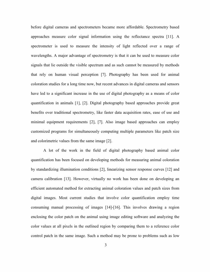
before digital cameras and spectrometers became more affordable. Spectrometry based

approaches measure color signal information using the reflectance spectra [11]. A

spectrometer is used to measure the intensity of light reflected over a range of

wavelengths. A major advantage of spectrometry is that it can be used to measure color

signals that lie outside the visible spectrum and as such cannot be measured by methods

that rely on human visual perception [7]. Photography has been used for animal

coloration studies for a long time now, but recent advances in digital cameras and sensors

have led to a significant increase in the use of digital photography as a means of color

quantification in animals [1], [2]. Digital photography based approaches provide great

benefits over traditional spectrometry, like faster data acquisition rates, ease of use and

minimal equipment requirements [2], [7]. Also image based approaches can employ

customized programs for simultaneously computing multiple parameters like patch size

and colorimetric values from the same image [2].

A lot of the work in the field of digital photography based animal color

quantification has been focused on developing methods for measuring animal coloration

by standardizing illumination conditions [2], linearizing sensor response curves [12] and

camera calibration [13]. However, virtually no work has been done on developing an

efficient automated method for extracting animal coloration values and patch sizes from

digital images. Most current studies that involve color quantification employ time

consuming manual processing of images [14]-[16]. This involves drawing a region

enclosing the color patch on the animal using image editing software and analyzing the

color values at all pixels in the outlined region by comparing them to a reference color

control patch in the same image. Such a method may be prone to problems such as low

4

repeatability of results, inter-observer error and reduced accuracy across time (observer

fatigue) over large datasets. As a result, there is a need for an automated framework that

provides fast, repeatable and efficient extraction of animal coloration values in digital

images.

Out of the many bright colored animal species studied as a part of animal color

quantification, the house finch (Haemorhous mexicanus) is an important one and has

been widely studied [17]-[19]. The house finches can have widely varying plumage

colors from bright red to orange–yellow. As stated earlier, these bright colors like red and

yellow are the result of carotenoid based pigments which are derived from the bird’s diet

[4]. Color measurements for the house finch can help researchers understand mating

success [20], [21] and the impact of environment on the quality of diet [1]. Fast moving

animal species such as the house finch need to be restrained by human hands during

image acquisition. The plumage color of the house finch is also very similar, at times, to

the color of the human hands holding the bird in place and this makes it much more

challenging to segment the plumage color of these birds. For these reasons, the house

finch is used as the main test subject in this study and its bright plumage color is used for

evaluating the performance of the proposed system.

1.2 Contributions

In this thesis, a novel perceptual-based approach for the automated extraction of animal

coloration variables such as hue, saturation, brightness, and patch size, from digital

images with slowly varying background colors, is presented. In this proposed framework,

the input image is first coarsely segmented into few classes using dominant colors. The

dominant colors are identified by detecting the local peaks in the image color distribution

5

computed in a perceptually uniform color space. The required foreground class is then

identified by eliminating the most dominant color in the color histogram of the image as

the color of the background region. In the case of fast moving animals, the animal

specimen is held in position by human hands. Therefore, to account for this latter case,

the foreground region is further segmented into skin and non-skin regions to identify the

region of human hands in the image. The skin/ non-skin classification is performed using

a Bayesian skin color classifier, with the required skin conditional density modelled as a

Gaussian mixture model. This is followed by an edge-enhanced model-based

classification scheme to eliminate the outlier skin regions. Finally, a novel perceptual-

based Saturation-Brightness quantization is implemented for the removal of perceptually

insignificant colors and only retaining the colors of interest (bright colors). The

perceptual based Saturation-Brightness quantization helps to refine the region of interest

by eliminating perceptually insignificant colors, such as black, gray and white while

preserving the perceptually visible (bright) colors. This perceptual-based quantization

step is useful for quantifying carotenoid pigment based colors and can be avoided if only

colors such as black, gray and white need to be quantified.

1.3 Thesis Organization

The organization of this thesis is as follows: Chapter 2 provides the background for the

different color spaces used for quantization, and basic concepts related to Bayes classifier

and Gaussian mixture models used for modelling conditional densities. Chapter 3

describes the current manual, semi-automated and automated methods that are related to

this thesis. Chapter 4 describes the proposed animal color extraction and quantification

framework. Chapter 5 presents performance results for a set of images, and a comparison

6

between the results produced by the proposed automated framework and manual scoring

methods. Chapter 6 summarizes the contributions of this thesis and proposes future

directions of research.

7

CHAPTER 2

BACKGROUND

This chapter provides some background information about the different color spaces used

in this thesis, Bayes classifier and Gaussian mixture modelling of multimodal

distributions, all of which is useful in understanding the implemented framework. Section

2.1 describes the different color spaces used in this framework. Section 2.2 explains the

expectation-maximization approach for deriving Gaussian mixture models. Section 2.3

describes Bayesian decision theory for classification.

2.1 Color Spaces

A color space is a multi-dimensional space representation that describes every color

produced by a color model as a unique tuple of three or four numbers called color

components. It is basically a combination of a color model that describes how various

observed colors can be produced and an associated mapping function that maps every

color to a unique point in a multi-dimensional space. The co-ordinates of such a point

represent the relative amounts of the individual color components of the considered color

model, which combine to produce the observed color. Usually, most color spaces use a

three-element tuple representation for colors and the 3 axes of the color space represent

the three fundamental color components of the color model used. Since a color space is

just a combination of a color model and a mapping function, many different combinations

of color models and mapping functions can be used to represent the same observed color.

8

In recent years, many different color space representations have been introduced

and the choice of a particular color space usually depends on the application. The various

color spaces are mainly divided into the following groups [22]:

a) Primary spaces

The primary spaces are based on the idea that every color can be produced by

mixing appropriate amounts of three primary colors.

b) Luminance-chrominance spaces

The luminance-chrominance spaces refer to color spaces in which one of the three

color space components represents luminance information and the other two

represent chrominance information.

c) Perceptual spaces

Perceptual spaces are designed to make color spaces more intuitive to humans. In

these color spaces, a color is represented by its hue, saturation and intensity, just

as a human would describe the same color.

d) Independent axis spaces

Independent axis color spaces are derived by using different statistical approaches

to minimize the correlation between the individual components of the color space.

In this section, we discuss the three different color spaces which are used in the

implemented framework. The three color spaces used are the CIE (R, G, B), the CIE (L*,

a*, b*) and the HSV color spaces.

2.1.1 CIE (R, G, B) color space

The CIE (R, G, B) color space is a primary color space based on the trichromatic theory,

which assumes that every color can be expressed as a combination of appropriate

9

Fig. 1 RGB color cube.

amounts of three primary colors. Analogous to the human eye, the three primary

components of the CIE (R, G, B) are red, blue and green. The color space is derived from

color matching experiments that were conducted using the three color primaries denoted

by Rc, Gc and Bc, which are monochromatic color signals of wavelengths 700.0 nm,

546.1 nm and 435.8 nm, respectively [22]. It is possible to obtain many different (R, G,

B) color spaces depending on the choice of wavelengths for the primaries. However, the

CIE (R, G, B) color space is considered as a reference (R, G, B) color space as it defines

the standard observer, whose eye spectral response represents the average eye spectral

response of a human observer [22]. Fig. 1 illustrates the RGB color cube which defines

the (R, G, B) color space and the three normalized vectors 𝑅𝑐⃗⃗⃗⃗ , 𝐺𝑐⃗⃗⃗⃗ and 𝐵𝑐⃗⃗⃗⃗ , which represent

𝐵𝑐⃗⃗⃗⃗

Green (0, 1, 0)

White (1, 1, 1)

Black (0, 0, 0)

Red (1, 0, 0)

Blue (0, 0, 1)

𝑅𝑐⃗⃗⃗⃗

𝐺𝑐⃗⃗⃗⃗

O

10

the three primaries (R, G, B). The normalized vectors 𝑅𝑐⃗⃗⃗⃗ , 𝐺𝑐⃗⃗⃗⃗ and 𝐵𝑐⃗⃗⃗⃗ form the principal

axes of the 3D vector space and intersect at the origin of the color space denoted by point

O. Every color is represented by a point C in the color cube and defined by a vector 𝑂𝐶⃗⃗⃗⃗ ⃗

with the projections of 𝑂𝐶⃗⃗⃗⃗ ⃗ on the primary axes representing the tristimulus values Rc, Gc

and Bc , which correspond to the relative amounts of the red, green, and blue primaries,

respectively, that combine to form the considered color. The tristimulus values for a

particular set of primaries are defined by color mapping functions, also known as color

matching functions. The normalized color matching functions for the CIE (R, G, B) color

space are denoted by �̅�(𝜆), �̅�(𝜆) and �̅�(𝜆). For a known set of color matching functions,

the normalized tristimulus (Rc, Gc, Bc) values for a color with power spectral distribution

I(λ) are given by [23]:

𝑹𝒄 = ∫ 𝐼(𝜆) �̅�(𝜆)𝑑∞

0λ (1)

𝑮𝒄 = ∫ 𝐼(𝜆) �̅�(𝜆)𝑑∞

0λ (2)

𝑩𝒄 = ∫ 𝐼(𝜆) �̅�(𝜆)𝑑∞

0λ (3)

The origin O with normalized tristimulus values (0, 0, 0) represents the color black and

the color white is defined by the normalized tristimulus values (1, 1, 1). The dotted gray

colored line in Fig.1 is known as the gray axis or the neutral color axis [22]. For every

point on this line, the x, y, and z co-ordinates are equal and as a result each point on this

line represents a different shade of gray between black and white. The primary colors red,

green and blue are given by (1, 0, 0), (0, 1, 0) and (0, 0, 1), respectively.

11

2.1.2 CIE (L*, a*, b*) color space (also known as CIELAB)

The (R, G, B) color space has a few drawbacks including the following:

a) The tristimulus values are dependent on the luminance, which is a linear

combination of the tristimulus values.

b) The (R, G, B) color spaces are device dependent and it is possible to formulate

many different (R, G, B) color spaces with different primaries and color matching

functions.

c) The (R, G, B) color spaces are not perceptually uniform.

Perceptual uniformity means that equal changes in color values should correspond to an

equal color difference perceived by a human.

To overcome the problem of perceptual non-uniformity and device dependence,

the CIE formulated an alternate perceptually uniform color space known as (L*, a*, b*)

or CIELAB. The (L*, a*, b*) color space is a luminance-chrominance space, where

unlike the (R, G, B) color space, the luminance (brightness) component is completely

separated from the chrominance (color) component of the input visual signal. The L*

component represents the brightness response of the human eye to a visual stimulus,

while the a* and b* components represent the green-red color opposition and blue-yellow

color opposition, respectively [22]. The forward transform that converts values in CIE

(R,G,B) color space to corresponding values in CIELAB color space is given by [24],

[𝑋𝑌𝑍] = [

0.49018 0.30987 0.199930.17701 0.81232 0.01066

0 0.01007 0.98992] [

𝑅𝑐𝐺𝑐𝐵𝑐

] (4)

L* = 116 ∗ 𝑓 (𝑌

𝑌𝑛) − 16 (5)

12

a* = 500 ∗ [𝑓 (𝑋

𝑋𝑛) − 𝑓 (

𝑌

𝑌𝑛)] (6)

b* = 200 ∗ [𝑓 (𝑌

𝑌𝑛) − 𝑓 (

𝑍

𝑍𝑛)] (7)

𝑓(𝑡) = {𝑡1

3, 𝑡 > (6

29)3

1

3(29

6)2

𝑡 +4

29, 𝑜𝑡ℎ𝑒𝑟𝑤𝑖𝑠𝑒.

(8)

where (Rc, Gc, Bc) represents the normalized tristimulus values in CIE (R, G, B) color

space, (X, Y, Z) represents tristimulus values in CIEXYZ color space, (Xn, Yn, Zn)

represents tristimulus values of the reference white point in CIEXYZ color space and (L*,

a*, b*) represents the corresponding tristimulus values in CIELAB color space.

Similarly, the backward transform that converts values from CIELAB to CIE (R, G, B)

color space is given by,

𝑌 = 𝑌𝑛 ∗ 𝑓−1 (

1

116(𝐿∗ + 16)) (9)

𝑋 = 𝑋𝑛 ∗ 𝑓−1 (

1

116(𝐿∗ + 16) +

1

500𝑎∗) (10)

𝑍 = 𝑍𝑛 ∗ 𝑓−1 (

1

116(𝐿∗ + 16) −

1

200𝑏∗) (11)

𝑓−1(𝑡) = {𝑡3, 𝑡 > (

6

29)

3 (6

29)2

(𝑡 −4

29) , 𝑜𝑡ℎ𝑒𝑟𝑤𝑖𝑠𝑒.

(12)

[

𝑅𝑐𝐺𝑐𝐵𝑐

] = [2.36353 −0.89582 −0.46771−0.51511 1.42643 0.088670.00524 −0.01452 1.00927

] [XYZ] (13)

2.1.3 (H, S, V) color space

Although the CIELAB color space is perceptually uniform, it is not very intuitive and

perceptually relevant for day-to-day applications of color systems such as graphics and

13

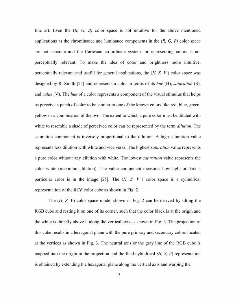
fine art. Even the (R, G, B) color space is not intuitive for the above mentioned

applications as the chrominance and luminance components in the (R, G, B) color space

are not separate and the Cartesian co-ordinate system for representing colors is not

perceptually relevant. To make the idea of color and brightness more intuitive,

perceptually relevant and useful for general applications, the (H, S, V ) color space was

designed by R. Smith [25] and represents a color in terms of its hue (H), saturation (S),

and value (V). The hue of a color represents a component of the visual stimulus that helps

us perceive a patch of color to be similar to one of the known colors like red, blue, green,

yellow or a combination of the two. The extent to which a pure color must be diluted with

white to resemble a shade of perceived color can be represented by the term dilution. The

saturation component is inversely proportional to the dilution. A high saturation value

represents less dilution with white and vice versa. The highest saturation value represents

a pure color without any dilution with white. The lowest saturation value represents the

color white (maximum dilution). The value component measures how light or dark a

particular color is in the image [25]. The (H, S, V ) color space is a cylindrical

representation of the RGB color cube as shown in Fig. 2.

The (H, S, V) color space model shown in Fig. 2 can be derived by tilting the

RGB cube and resting it on one of its corner, such that the color black is at the origin and

the white is directly above it along the vertical axis as shown in Fig. 3. The projection of

this cube results in a hexagonal plane with the pure primary and secondary colors located

at the vertices as shown in Fig. 3. The neutral axis or the gray line of the RGB cube is

mapped into the origin in the projection and the final cylindrical (H, S, V) representation

is obtained by extending the hexagonal plane along the vertical axis and warping the

14

Fig. 2 HSV model representation using cylindrical co-ordinates.

Fig. 3 Projection of tilted RGB cube on a plane.

120 degrees

Value

Hue

Saturation

0 degrees

240 degrees

15

hexagon into a circle. The hue is the angle of the vector formed by the projection of a

point in the RGB cube onto the hexagonal plane, measured about the vertical axis with

red at 0°, green at 120° and blue at 240°. The saturation is measured along the radius of

the cylinder over a range of [0, 1] as shown in Fig. 2. The value component forms the

vertical axis of the cylindrical representation, with a range of values between [0, 1]. All

points that lie on the vertical axis have a saturation component equal to zero and as a

result have no color information associated with them. These points represent the

different shades of gray between black and white and have no specific value of hue

defined for them. As these points have no unique hue value defined for them, it is

possible to identify and represent shades of gray including black and white in this color

space by just computing the saturation and value components, independent of the hue

component. Black can be represented by the point {S=0, V=0}, while white is

represented by {S=0, V=1} and shades of gray are represented by points {𝑆 = 0, 0 ≤

𝑉 ≤ 1} on the vertical axis. The transformation of normalized tristimulus (Rc, Gc, Bc)

values to (H, S, V) values is given by [25]:

𝐶 = max(𝑅𝑐, 𝐺𝑐, 𝐵𝑐) − min (𝑅𝑐, 𝐺𝑐 , 𝐵𝑐) (14)

𝐻 =

{

60

° ∗ (𝐺𝑐−𝐵𝑐

𝐶mod(6)) , if max (𝑅𝑐, 𝐺𝑐, 𝐵𝑐) = 𝑅𝑐

60° ∗ (𝐵𝑐−𝑅𝑐

𝐶+ 2) , if max (𝑅𝑐, 𝐺𝑐, 𝐵𝑐) = 𝐺𝑐

60° ∗ (𝑅𝑐−𝐺𝑐

𝐶+ 4) , if max(𝑅𝑐, 𝐺𝑐, 𝐵𝑐) = 𝐵𝑐

𝑢𝑛𝑑𝑒𝑓𝑖𝑛𝑒𝑑 𝐶 = 0

(15)

𝑆 = { 0, 𝐶 = 0𝐶

max (𝑅𝑐,𝐺𝑐,𝐵𝑐), otherwise. (16)

𝑉 = max (𝑅𝑐, 𝐺𝑐, 𝐵𝑐) (17)

16

𝑥𝑚𝑜𝑑(𝑦) = 𝑥 − ⌊𝑥

𝑦⌋ ∗ 𝑦 (18)

where ⌊𝑥

𝑦⌋ represents a flooring operation in which the quotient of

𝑥

𝑦 is rounded

downwards.

2.2 Gaussian Mixture Model Estimation using Expectation-Maximization

In most classification problems, the conditional probability densities cannot be accurately

represented as unimodal distributions and usually take the shape of complex multi-modal

distributions. A Gaussian Mixture Model (GMM) is a parametric probability distribution

function that is widely used for modelling such complex shaped multi-modal

distributions. The GMM is a weighted sum of multiple unimodal component Gaussian

densities given by the equation,

𝑝(𝑥) = ∑ 𝑤𝑖 𝑚𝑖=1 𝑔(𝑥|𝜇𝑖, Σ𝑖) (19)

where x is an N-dimensional vector, wi is the mixture weight and 𝑔(𝑥|𝜇𝑖, Σ𝑖) is the

component density for the ith Gaussian component. The component density is given by,

𝑔(𝑥|𝜇𝑖 , Σ𝑖) =1

(2𝜋)𝑁/2|Σ𝑖|1/2 exp {−

1

2(𝑥 − 𝜇𝑖)

𝑇𝛴𝑖−1(𝑥 − 𝜇𝑖)} (20)

where 𝜇𝑖 and Σ𝑖 represent, respectively, the mean vector and covariance matrix of the ith

component density. The mixture weights also satisfy the following constraint:

∑ 𝑤𝑖𝑚𝑖=1 = 1 (21)

Due to the parametric nature of the model, the entire model can be accurately represented

using just the mean vector 𝜇𝑖, covariance matrix Σ𝑖 and mixture weight wi for each

component Gaussian density and these parameters can be estimated from a training data

set using a maximum-likelihood approach.

17

The GMM parameters are estimated iteratively, using a special case of the

Expectation-Maximization algorithm [26]. Given an initial estimate of the GMM model,

the E-M algorithm iteratively estimates a model 𝜆, such that 𝑝(𝑋|𝜆𝑡+1) ≥ 𝑝(𝑋|𝜆𝑡) at

iteration t+1 for a given training set X={x1, x2,…..,𝑥𝑇1} with 𝑇1 training samples. 𝜆

represents the set of component parameters {𝑤𝑖, 𝜇𝑖, Σ𝑖} for the M component densities.

The likelihood 𝑝(𝑋|𝜆𝑡+1), posterior probability, mean vector, covariance matrix and

mixture weight is recomputed for all components at every iteration till a stopping criteria

that maximizes the likelihood function is reached. At every iteration, the posterior

probability for each component and training sample is first calculated as:

𝑃𝑖,𝑗(𝑡)=

𝑤𝑖(𝑡)𝑔(𝑥𝑗|𝜇𝑖

(𝑡),Σ𝑖(𝑡))

∑ 𝑤𝑘(𝑡)𝑚

𝑘=1 𝑔(𝑥𝑗|𝜇𝑘(𝑡),Σ𝑘(𝑡)) (22)

where t represents the iteration number, i represents the component number and xj is the

jth training sample in X. Next, the updated mean vector, covariance matrix and mixture

weight for the ith component are calculated as:

𝑤𝑖(𝑡+1)

=1

𝑇1∑ 𝑃𝑖,𝑗

(𝑡)𝑇1𝑗=1 (23)

𝜇𝑖(𝑡+1)

=∑ 𝑃𝑖,𝑗

(𝑡)𝑥𝑗

𝑇1𝑗=1

∑ 𝑃𝑖,𝑗(𝑡)𝑇1

𝑗=1

(24)

Σ𝑖(𝑡+1)

=∑ 𝑃𝑖,𝑗

(𝑡)(𝑥𝑗−𝜇𝑖

(𝑡+1))(𝑥𝑗−𝜇𝑖

(𝑡+1))𝑇𝑇1

𝑗=1

∑ 𝑃𝑖,𝑗(𝑡)𝑇1

𝑗=1

(25)

𝐿(𝑥; 𝜆𝑡+1) = ∏ 𝑝(𝑥𝑗|𝜆𝑡+1)𝑇1𝑗=1 (26)

where 𝜆𝑡+1 represents the model for iteration t+1 and 𝐿(𝑥; 𝜆𝑡+1) represents the likelihood

function at iteration t+1. The E-M algorithm is terminated when the difference between

ln𝐿(𝑥; 𝜆𝑡+1) and ln𝐿(𝑥; 𝜆𝑡)is lesser than a pre-decided threshold.

18

2.3 Bayesian Decision Theory

Bayesian decision theory is an important statistical approach used in many pattern

classification tasks. The approach uses a probability distribution to evaluate the merit of

various classification decisions along with the cost associated with making each

classification decision. This approach assumes that a particular classification task can be

formulated as a problem based on probability and, given all the relevant conditional

densities and prior probabilities, predicts the best classification rule as the one that

minimizes the probability of error [27].

For an object classification task, a classification can be performed by assigning

the observed object to the class wi with the highest a priori probability P(wi). However, a

measured value or feature x that represents an attribute of the object can be used to make

a more robust decision that minimizes the probability of error. The measured value x can

be a single value or a vector of values representing a feature. Consider a general

classification problem where we have a measurement value x which is continuous and the

classification scheme has to identify the class wi, i = 1, 2, 3,…..,M, that produced the

measurement x. The a priori probabilities represented by P(wi), i = 1, 2, 3,….., M, and the

likelihood functions or class conditional densities represented as 𝑝(𝑥|𝑤𝑖), i = 1, 2, 3,…..,

M, are assumed to be completely known. The probability of error associated with the

object being assigned to class wj, given a measurement x is given as:

𝑃(𝑒𝑟𝑟𝑜𝑟|𝑥) = ∑ 𝑃(𝑤𝑖𝑀𝑖=1,𝑖≠𝑗 |𝑥). (27)

This can be re-written in another form as,

𝑃(𝑒𝑟𝑟𝑜𝑟|𝑥) = 1 − 𝑃(𝑤𝑗|𝑥) (28)

due to the relation, ∑ 𝑃(𝑤𝑖|𝑥)𝑀𝑖=1 = 1. The average probability of error is given by:

19

𝑃(𝑒𝑟𝑟𝑜𝑟) = ∫ 𝑃(𝑒𝑟𝑟𝑜𝑟|𝑥)𝑝(𝑥)𝑑𝑥∞

−∞ (29)

where 𝑝(𝑥) can be expressed as follows:

𝑝(𝑥) = ∑ 𝑝(𝑥|𝑤𝑖𝑀𝑖=1 )𝑃(𝑤𝑖). (30)

As per Bayes’ decision theory, the best decision chooses the class that minimizes (27).

From (28), we observe that 𝑃(𝑒𝑟𝑟𝑜𝑟|𝑥) is minimized when 𝑃(𝑤𝑗||𝑥) is maximized. Thus

the best decision chooses the class 𝑤𝑗 for which 𝑃(𝑤𝑗|𝑥) is maximum. Using Bayes’

theorem, we can write 𝑃(𝑤𝑗|𝑥) as,

𝑃(𝑤𝑗|𝑥) =𝑝(𝑥|𝑤𝑗)𝑃(𝑤𝑗)

𝑝(𝑥). (31)

Since 𝑝(𝑥) is just a scaling factor and is the same for all classes, we can ignore 𝑝(𝑥) to

get the final form of the Bayes’ decision theory. For an M class classifier, given a

measurement x, the Bayes classifier chooses the class 𝑤𝑗 such that:

𝑝(𝑥|𝑤𝑗)𝑃(𝑤𝑗) ≥ 𝑝(𝑥|𝑤𝑖)𝑃(𝑤𝑖) ∀𝑖 ≠ 𝑗. (32)

The expression in (28) can be further simplified for a binary classifier with equal prior

probabilities for both classes. In this latter case, for a given measurement x, we decide to

choose class 𝑤1 if

𝑝(𝑥|𝑤1) ≥ 𝑝(𝑥|𝑤2) (33)

and class 𝑤2 otherwise.

20

CHAPTER 3

RELATED WORK

This chapter summarizes the previous work related to animal coloration quantification

methods using digital photography. Section 3.1 describes few popular manual software

methods. Section 3.2 describes an automated approach for intensity quantification of

animal patterns in gray scale images.

Digital image processing and computer vision approaches have been widely used

for many automated image and video analysis applications such as biometrics,

biomedical imaging, microscopy, surveillance etc. For example, automated image

processing methods have been implemented for face, fingerprint recognition and

matching [28], cell migration in microscopy images [29], identifying and tracking people

and objects in videos for surveillance, computer aided lesion detection and diagnosis in

mammography [28] etc. The range of applications for automated image analysis is ever

expanding.

There has been a steady increase in the use of digital photography for quantifying

animal and plant color patterns in recent years [2], [30], [31], due to the fast data

acquisition speeds and permanent storage capability provided by it [2]. The use of digital

photography in coloration studies also allows for multi-parameter measurements and

enables researches to obtain measurements in the wild without the trouble of managing

expensive and bulky equipment. Although digital photography provides several useful

benefits over traditional animal coloration quantification approaches like spectrometry

[7], [2], it does have a few important limitations that affect the accurate measurement and

quantification of coloration in animals. Digital camera sensors have non-linear intensity

21

response curves and the colors reproduced in images are device-dependent due to the

variation in spectral responses of different camera sensors [2]. As a result, if not corrected

for these effects, the same image acquired using different digital cameras would provide

different color quantification results. Also, a lot of the recent digital cameras employ built

in image pre-processing and compression algorithms that modify the initial raw intensity

data recorded by the camera.

In order to better leverage the benefits of digital photography, work has been done

on developing methods for measuring animal coloration by standardizing illumination

conditions [2], linearizing sensor response curves [12] and camera calibration [13].

However, the idea of implementing an efficient and robust automated software

framework for quantifying animal coloration has largely been unexplored [2].

3.1 Manual Software Methods

The most popular and widely used current manual method involves the use of a digital

photo editing software like Adobe Photoshop [32], GIMP [33], ImageJ [34] etc. with

user-driven inputs to identify the region of interest (henceforth referred to as ROI) and

quantify it [35]. The ROI is identified by using a magic wand tool that takes user-

provided locations for identifying the ROI. After an initial start location is provided in the

image by the user, the software implements a region growing method to merge regions

around the user-provided start location, based on the similarity of color. The sensitivity of

the region merging process to color differences is controlled by a threshold and the ROI

is refined by repeated readjustments of this threshold by the user. The color quantification

is achieved using histogram based tools or external plugins provided for measuring image

intensities in these software packages. The method illustrated in [35] can be considered as

22

a semi-automated method as opposed to the prior manual methods of actually drawing a

contour tightly enclosing the ROI using a freehand region drawing tool [14]-[16].

Identifying the ROI by drawing a closed contour around it using a freehand drawing tool

in an image editing software is an extremely cumbersome task, may provide low

repeatability of results and the accuracy of results is largely user dependent. The semi-

automated user-driven method in [35] explained earlier, uses a user driven region

merging process and is more robust and accurate as compared to the manual method of

selecting the region of interest using a freehand drawing tool. However, the software

based semi-automated method also has many limitations. The semi-automated user-

driven method can be extremely time consuming, does not provide batch processing

capabilities and can result in low intra-photo repeatability. Also, since the region growing

process is user controlled, the accuracy of results may be significantly reduced over large

datasets, due to user fatigue.

Vortman et al. [36] developed a couple of user-driven MATLAB based software

packages called “Hirundo” and “Hirundo feather” for measuring animal coloration and

feather coloration. Unlike the user-driven region growing/merging method used in [35],

the “Hirundo” tool is based on the idea of two-class quantization of the user selected

region to measure the color values of interest. In this method, the user selects a

rectangular region enclosing the ROI and the software tool then performs a two-class

quantization of the selected region into foreground (ROI) and background. The authors in

[36] claim to use a Lloyd-Max quantizer based algorithm for this quantization and a user-

defined threshold for adjusting the image region considered to be foreground. However,

the authors in [36] do not provide any further details about their quantization scheme.

23

Given that the Lloyd-Max quantizer is used for generating optimal partitions of

continuous geometric regions and the quantization scheme results in [36] can be adjusted

using user-defined thresholds, it is unlikely that the Lloyd – Max quantization is being

used in the approach in [36]. It is more likely that the quantization of the user-selected

region in [36] is performed using just a user-defined threshold, to get the desired ROI.

Although using the “Hirundo” tool is not as cumbersome as the method in [35], it suffers

from the same limitations as [35]. The requirement of a user-defined region for

quantization makes this approach both time consuming and susceptible to inter-observer

errors. Also, if the ROI consists of more than one quantifiable color (e.g., Butterfly wing

patterns), the two-class quantization process is unable to quantify them separately and the

resultant chrominance values of the ROI would correspond to an average of the

chrominance values of the quantifiable colors. Such an average value would represent a

totally different color than the one to be quantified. For example, if the identified ROI

consisted of red and green colored regions, then the tool would most likely provide a

quantified chrominance value corresponding to the color yellow. These limitations

necessitate the development of an automated framework that is able to automatically

characterize multiple colors in the scene in a fast manner, with a high-degree of accuracy

and avoid human and inter-observer errors.

3.2 Automated Quantification Method

As mentioned before, most of the research in using digital photography methods for

quantifying animal coloration have focused on optimizing the conditions for acquiring

images, linearizing camera sensor responses and camera calibration. Virtually no work

has been done on implementing a flexible framework for automatically segmenting and

24

quantifying the different animal coloration patterns in digital images. A couple of

approaches for segmenting simple animal coloration patterns in grayscale images, using

basic image processing methods such as intensity based thresholding and edge based

thresholding were proposed in [2]. In the first approach, the ROI is segmented by

converting the 8-bit grayscale image into a binary image using a user-defined threshold,

where every pixel belonging to the ROI is assigned a value of 1 and all other pixels are

assigned a value of 0. The required threshold value is decided based on prior knowledge

of the area to be segmented or some explicit assumption. The second approach uses

strong edges to identify the region of interest. This approach is based on the assumption

that the boundary of the ROI corresponds to the sharp changes in intensity in an image.

These sharp changes in intensity can be identified by detecting the strong edges in the

image. Both of these approaches assume some prior knowledge of the data for computing

the threshold values and are not designed to segment complex region boundaries found in

many animal coloration studies. In contrast, the proposed framework in this thesis

assumes no prior knowledge of the location or color of the specimen used for color

quantification.

25

CHAPTER 4

IMPLEMENTED AUTOMATED COLOR QUANTIFICATION SYSTEM

This chapter describes the proposed framework for automated animal coloration

extraction and quantification in digital images. The developed framework consists of 4

major steps: extracting the foreground region and excluding the background region using

dominant colors, skin/non-skin region classification using a binary Bayesian classifier,

removal of outlier skin pixels using an edge-enhanced model, and perceptual-based

Saturation-Brightness quantization to refine the region of interest by eliminating

perceptually insignificant colors, such as black, gray and white, while preserving the

perceptually visible (bright plumage) colors. Section 4.1 presents an overview of the

implemented automated animal coloration quantification system. The four major

components of the proposed animal coloration quantification framework are described in

Sections 4.2 to 4.5. Section 4.6 describes the MATLAB-based software implementation

and summarizes the major steps of the proposed algorithm.

4.1 Overview of the Proposed System

In this work, the problem of extracting the animal coloration patches is treated as a color

segmentation problem and the proposed approach draws inspiration from the class of

image segmentation methods that use a few representative dominant colors for

segmenting an image into regions of perceptually homogenous colors.

In many images used for animal color quantification, a standard color strip is

placed alongside the bird or animal as shown in Fig. 4. The strip can be used for

illumination correction in post-acquisition analysis. In this work, the color strip is

26

Fig. 4. Original image with the color strip present.

Fig. 5. Binary image showing the detected color square in white, for color strip removal.

27

Fig. 6. Image obtained after removing the color strip from the image.

detected by searching for the presence of a specific color present in the color strip, using

a MMSE (minimum mean squared error) metric. Once the color strip is detected, its

color(s) can be quantified and stored for use in color normalization to achieve an

illumination-invariant color quantification. Since the color strip is outside the Region-of-

Interest (ROI) containing the animal, a cropped image containing the ROI is formed by

removing the region containing the detected color strip. Fig. 4 shows the image before

color strip removal. The binary mask showing the detected color square in white, used for

color strip removal, is shown in Fig. 5. The image after color strip removal is shown in

Fig. 6. After color strip removal, the cropped image is processed by the proposed

automated animal coloration quantification algorithm (see more below) to extract and

quantify the colors in the ROI. In the remainder of this thesis, the term input image refers

to the image after color strip removal. Fig. 7 illustrates the block diagram of the proposed

algorithm. After color strip removal, a coarse two-class color quantization is performed

on the input image in order to segment the image into a background (insignificant region)

and a foreground (region containing the object of interest) region.

28

Fig. 7 Block diagram of the proposed framework.

The extracted foreground region is then further processed in order to extract

colors corresponding to the bird plumage area, while removing other outlier colors such

as colors due to the presence of human hands with or without gloves. If gloves are used,

removing the outlier colors is a relatively easy task since the color of the gloves is

typically chosen to be significantly different than the colors of interest in the animal. The

gloves can be removed using a coarse color quantization scheme similar to the one used

in the aforementioned foreground extraction step. If no gloves are used, the problem

becomes more challenging since the human skin color can be in many cases similar to the

colors of interest in the animal. In order to eliminate the regions corresponding to the

human skin colors while preserving the bright animal colors, we propose a novel model-

based approach combined with a Bayesian classifier. After regions corresponding to

29

human skin are removed, the remaining foreground region is subjected to a perceptual-

based saturation-brightness quantization that preserves the perceptually visible colors

(bright colors like red, yellow, orange etc.) while removing the perceptually insignificant

ones. The resulting ROI colors are quantified in terms of their mean hue, saturation and

brightness values for each segmented color patch in the ROI. The size of each ROI color

patch is also provided as an output by the proposed algorithm. Further details about the

foreground extraction and background removal, skin/non-skin classification, edge-

enhanced model-based outlier skin pixel removal and perceptual-based Saturation-

Brightness quantization are presented in Sections 4.2 to 4.5 .

4.2 Foreground Extraction and Background Removal using Dominant Colors

As previously mentioned, most coloration analysis images usually include a reference

color strip to correct for non-standard illumination conditions. Since the color strip does

not provide any useful information to the task of segmenting the area of interest, we

choose to detect and remove the color strip from the image by cropping it. This helps to

improve the computation time by reducing the number of pixels used for further

processing. After color strip removal and image cropping, a foreground extraction

process is implemented on the input image to remove background regions. The

foreground-background extraction is performed by assigning each pixel in the image to

either a background or foreground region (also referred to as class or cluster) based on

the pixel color. This process is a two-class (background/foreground) color quantization of

the image color space and can be achieved using any of the several color space

segmentation approaches available in the literature such as mean-shift clustering [37],

Gaussian mixture model based classification [38], k-means clustering [38], color

30

quantization methods used in display devices [39] etc. In this proposed work, the

foreground–background classification is performed using a k-means clustering algorithm.

However, it is well known that using an unsupervised k-means clustering approach is

extremely sensitive to the choice of initial seeds (initial representative color for each

cluster). Better results can be achieved by using user-provided or intelligently derived

initial seeds as compared to a random selection of initial seeds [40]. In this work, we are

interested in an automatic initial seed selection process rather than user-provided seeds.

For this purpose, we propose the use of dominant colors in the image as the initial seeds

for the k-means clustering.

4.2.1 Dominant color extraction in images

Ma et al. [41] proposed the idea of using dominant colors for a concise color space

representation for image segmentation and a number of different approaches for

dominant color extraction have been proposed [41]-[45]. In this work, the dominant

colors in the image are automatically identified by computing the color distribution of the

image content. The dominant colors are determined by locating local peaks or modes in

the image color distribution using the mean-shift mode detection as in [37]. The use of a

few important colors to represent the image color distribution helps in merging regions of

similar color into a single abstraction that aids the task of ROI segmentation. Before

computing the dominant colors in the image, the input image is convolved with a

Gaussian smoothing filter in order to remove noise and merge very small regions of color

with the nearest larger color cluster. This helps to reduce the number of unique colors in

the image and speed up mode detection. Another approach to reduce the number of

unique colors is to quantize an 8 bit three channel RGB image to a 5 bit three channel

31

image by ignoring the last 3 bits of every 8 bit pixel value in the image [39]. Such a

preprocessing step can reduce the maximum number of unique colors possible in an RGB

image from 2563 to just 323 with very little loss in quality for the considered application.

An important factor that affects the color segmentation results is the choice of

color spaces. As discussed in Chapter 2, the RGB color space is perceptually non-

uniform, i.e., a small perceptual difference between two colors can correspond to a large

distance in the color space and vice versa [22]. Since the Euclidean distances used to

measure color differences in these non-perceptually uniform color spaces do not

correspond to human perceived color differences, the RGB color space is not the best

choice for image segmentation methods aimed at emulating human visual perception. It

has been shown that the performance of color segmentation methods is greatly improved

by using perceptually uniform color spaces such as the ones recommended by the CIE

[46]. In this work, the perceptually uniform L*a*b* (also known as CIELAB) color

space, described in Section 2.1.2 of Chapter 2, is used for representing the color

distribution of the considered images as it provides a perceptually uniform representation

of colors [37], [42], [46]. This helps to ensure that perceptually similar colors are grouped

in the same segmentation class. Also, since the luminance L* and chrominance a*b*

components in the L*a*b* color space are separated, we only need to consider the a* and

b* color components for extracting the dominant colors in the image as compared to the

R, G and B components in the RGB color space. This reduces the complexity of the

dominant color extraction process as well as the k-means clustering process.

32

Fig. 8. Original image containing multiple colors.

Fig. 9. Image Segmentation result using 14 dominant colors.

33

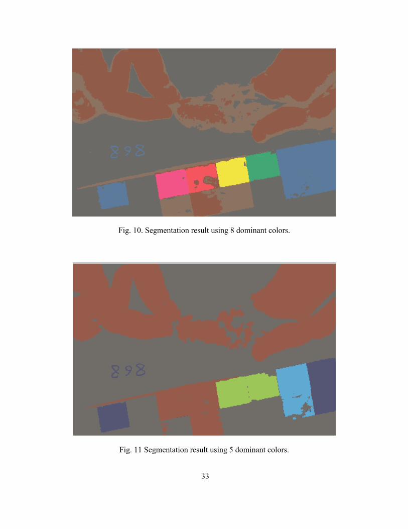
Fig. 10. Segmentation result using 8 dominant colors.

Fig. 11 Segmentation result using 5 dominant colors.

34

We first generate an L*a*b* space mapping of the colors in the image and then

compute a 2-D color histogram of the image, where the chrominance components a* and

b* represent the dimensions of the 2-D color histogram. The dominant colors are then

determined by detecting modes (local peaks) in the histogram as indicated previously.

The number of dominant colors detected also affects the accuracy of segmentation

results. Using a large number of colors results in over-segmentation of the image, while

using very few colors results in under-segmentation of the image and parts of the region

of interest being assigned to the background class. In the proposed framework, the

number of colors detected is adaptive and depends on the size of the window used for

mode detection. The size of the window is chosen to be a factor of the total variance of

the image color space. Fig. 8 shows the original image, while Fig. 9, Fig. 10 and Fig. 11

show image segmentation results using different number of dominant colors such as 14, 8

and 5 dominant colors, respectively.

4.2.2 Foreground extraction using k-means clustering

After extracting the dominant colors of the image, a k-means clustering operation is

performed as described earlier, on the color values using the a* and b*component values

for each pixel in the image to produce a multi-class abstraction of the image, with the

number of classes produced being equal to the number of dominant colors detected

previously. Since the background has an almost homogenous color and occupies the

largest portion of the total image area, the background cluster is identified as the cluster

whose center is closest to the largest peak in the image color distribution, which

corresponds to the background dominant color. Pixels in a particular dominant color

35

Fig. 12. Input image.

Fig. 13. Foreground-background class abstraction for the image shown in Fig. 12;

foreground region shown in white.

cluster are assigned to the background cluster based on how close their cluster center is to

the background cluster center and this is evaluated by taking the Euclidean distance

between the candidate cluster center and the identified background cluster center. All

pixels in a cluster are labeled as background pixels, if the Euclidean distance between

their cluster center and the background cluster center is less than a certain threshold. The

value of the threshold used in this work is equal to 12. The remaining pixels are labeled

as foreground pixels. This results in the segmentation of the image into a background

region that is ignored and a foreground region that is processed further. Fig. 13 shows the

36

resulting foreground-background segmentation mask for the input image shown in Fig.

12, where the white and black regions correspond, respectively, to the extracted

foreground and background regions.

4.3 Skin/Non Skin Region Classification

In images involving color quantification of live, fast moving animals, the specimen is

held in position by human hands. Since we initially segment the image into just two

classes, the region corresponding to human hands in the image may also be retained in

the foreground class as shown in Fig. 13. Since no prior knowledge about the color of the

ROI is assumed before the start of segmentation, a foreground - background classification

based on dominant colors is not enough to accurately extract the ROI. In order to

differentiate the ROI from the region corresponding to human hands in the image, the

foreground class needs to be further segmented. We achieve this segmentation by first

using a Bayesian skin color classifier [47], which segments the foreground class into

candidate skin and non-skin pixels on the basis of chrominance values for each pixel.

In order to use the Bayesian classifier for human skin classification, we first

need to estimate the class conditional probabilities from a sample dataset of skin and non-

skin images. The conditional probability distributions for the skin and non-skin classes

can be modeled each in color space as single bivariate Gaussian distributions as shown in

[47], [48], [49] and as Gaussian mixture density models as shown in [49], [50], [51]. Two

important factors for implementing an efficient skin detector are:

(i) The amount of overlap between the skin and non-skin distributions and the shape of

the distributions in a given color space.

37

(ii) The ability of a probabilistic model to approximate a complex-shaped distribution in a

given color space.

In the proposed framework, the perceptually uniform CIELAB (L*, a*, b*) space is used

to model the skin and non-skin conditional densities. The skin color distribution in such

perceptually uniform spaces usually takes the shape of a complex multi-modal

distribution. To effectively model such a complex shaped distribution, a Gaussian

mixture model is used in this framework. The Gaussian mixture model is estimated by

implementing the approach mentioned in Section 2.2 on a sample data set consisting of

500 images of size 60x60 pixels each, with 250 images for the skin class and 250 images

for the non-skin class. This results in a total of around 2 million pixel color values. The

images are transformed to the CIELAB space and the Expectation-Maximization

algorithm is implemented using the entire dataset. Fig. 14 shows sample images from the

skin dataset.

The number of components in a Gaussian mixture model is usually assumed to

be known. In general, increasing the number of parameters tends to increase the

likelihood but also leads to over-fitting. To determine the exact number of components

needed for a given data distribution, an information criteria such as the Akaike

Information Criterion (AIC) or AIC with correction (AICc) can be used. Such

information criteria assign a penalty term for the number of components to balance the

tradeoff between maximizing the likelihood and over-fitting. The AIC gives the optimal

number of components under asymptotic conditions. The AIC is given by the equation

[52],

𝐴𝐼𝐶 = 2𝑘 − 2ln (𝐿) (34)

38

Fig. 14 Sample images from the skin dataset used to estimate the skin condition.

39

where k is the number of free parameters in the model and L is the maximized value of

the likelihood function for the estimated model. For a Gaussian mixture model with M

bivariate Gaussian components having symmetric non-diagonal covariance matrices, the

number of free parameters k =(6𝑀 − 1) [53]. The AIC is computed for a set of candidate

models and the model that produces the minimum AIC value is chosen as the model with

the optimal number of components [52]. For the skin color dataset used in this work, an 8

component Gaussian mixture model provided good results. As discussed in Section 2.2,

the initial estimates for the mean vectors and covariance matrices of the Gaussian

components are obtained by a vector quantization of the color space distribution. The

skin class conditional can be obtained from (16) by choosing M=8 and is given by:

𝑝(�̅�(𝑖, 𝑗)|𝑆 = 1) = ∑ 𝑤𝑖 8𝑖=1 𝑔(𝑥|𝜇𝑖, Σ𝑖) (35)

where 𝑔(𝑥|𝜇𝑖, Σ𝑖) is a bivariate Gaussian density function as described in (17), 𝜇𝑖 and Σ𝑖

represent, respectively, the mean vector and covariance matrix, the vector �̅� (𝑖, 𝑗) = [a*(i,

j) b*(i, j)]T represents the chrominance values (a*,b*) for the pixel at coordinates (i, j)

and S is used to represent the skin class for S=1 and the non-skin class for S=0. The non-

skin distribution is modelled as a single bivariate Gaussian density function and is given

by,

𝑝(�̅�(𝑖, 𝑗)|𝑆 = 0) = 𝑔(𝑥|𝜇𝑖, Σ𝑖) (36)

where 𝑔(𝑥|𝜇𝑖, Σ𝑖) is same as described in (17). The non-skin distribution can also be

modelled as a Gaussian mixture model, but a single Gaussian provided good results for

the tested images.

Using the class conditional densities defined earlier, a two class Bayesian classifier,

as explained in Section 2.3 is implemented, and classifies every pixel in the foreground

40

class as skin or non-skin pixel. Given a chrominance vector �̅� ( 𝑖, 𝑗) = [a*(i, j) b*(i, j)]T

for an image pixel at coordinates (i, j), and assuming equal prior probabilities for both the

skin and non-skin class, the classifier classifies this pixel as a skin pixel if,

𝑝(�̅�(𝑖, 𝑗)|𝑆 = 1) ≥ 𝑝(�̅�(𝑖, 𝑗)|𝑆 = 0) (37)

A binary mask S(i,j) is produced by the Bayesian classifier where S(i,j)=1 corresponds to

a candidate skin pixel at location (i,j), and S(i,j)=0 corresponds to a non-skin pixel.

4.4 Edge-Enhanced Model-Based Classification for Outlier Pixel Removal

As mentioned in Section 4.3, the foreground region needs to be segmented into a skin and

a non-skin class in order to remove the region corresponding to human hands in the

foreground class. The accuracy of a human skin classifier based on chrominance only,

largely depends on the amount of overlap between the class conditional densities of the

skin and non-skin classes in the color space and the number of samples in each of the

training sets for each class [49]. This thesis work focuses on a broad set of images

consisting of different species of animals used in coloration analysis instead of a single

species of animals. As a result, no assumption regarding the color of the specimen is

made in this approach, except that the background is chosen to be different than the

colors of interest of the animal. As illustrated in Fig. 12, it is possible that the color of the

ROI is perceptually similar to the color of human hands. In such a case, the candidate

skin pixels determined by the skin classifier might not all correspond to true skin pixels

since some plumage colors might be similar to skin color and a skin color classifier may

not be sufficient to effectively identify the ROI. To circumvent this problem, the

candidate skin pixels that are obtained using the color-based Bayesian classifier are

41

further refined into skin and non-skin regions by using the edge information that is

present in the luminance component of the considered image. Our model-based approach

is based on the assumptions that 1) the region of human hands can be separated from an

ROI having a perceptually similar color by using the luminance component of the image

due to a perceivable difference in the luminance values of the hand region and the ROI,

resulting in a significant or strong edge at the hand-ROI interface; and 2) the region of

human hands is connected to the acquired image border as illustrated in Fig. 12. The first

assumption helps in separating the similar colored hand region from the ROI if these are

connected (Fig. 12). The second assumption helps in identifying and removing the hand

region from the foreground. Removing directly the region connected to the border

without initially separating the true hand region from the misclassified skin pixel regions

in the ROI will result in the removal of parts of the ROI which are misclassified as skin

pixel regions. Thus, in the proposed approach, an edge map is first generated and is used

to separate the true hand region from the misclassified skin pixel regions in the ROI. The

region that is connected to the image border is then determined as the true human hand

region and removed from the foreground region in Fig. 13, resulting in the final ROI

mask.

The Canny edge gradient operator [54] is used to first generate an edge gradient

magnitude image. Other suitable edge detectors can also be used for this purpose. A

binary edge map representing the strong edges in the image is generated from the edge

gradient magnitude image using a thresholding operation. Pixels that form a strong edge

are represented by a value of 1 in the binary edge map. We compute the threshold 𝑡ℎ𝑖𝑔ℎ

for the Canny edge detector using a histogram of the edge gradient magnitudes. The

42

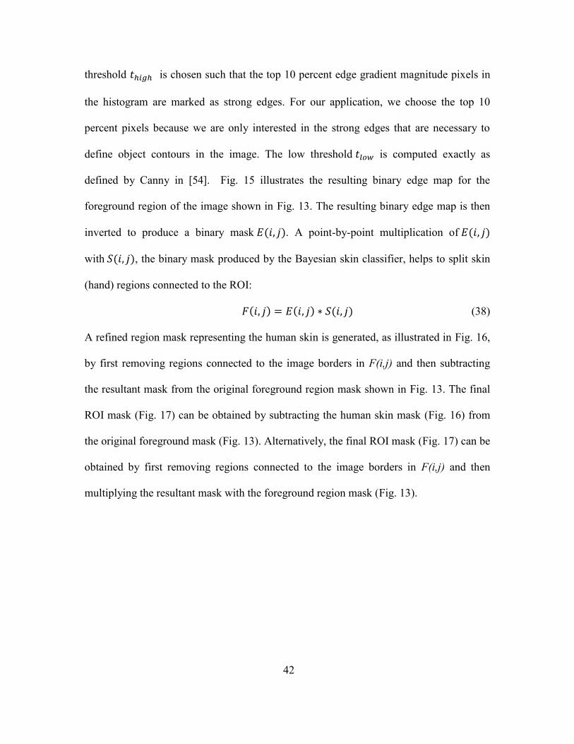
threshold 𝑡ℎ𝑖𝑔ℎ is chosen such that the top 10 percent edge gradient magnitude pixels in

the histogram are marked as strong edges. For our application, we choose the top 10

percent pixels because we are only interested in the strong edges that are necessary to

define object contours in the image. The low threshold 𝑡𝑙𝑜𝑤 is computed exactly as

defined by Canny in [54]. Fig. 15 illustrates the resulting binary edge map for the

foreground region of the image shown in Fig. 13. The resulting binary edge map is then

inverted to produce a binary mask 𝐸(𝑖, 𝑗). A point-by-point multiplication of 𝐸(𝑖, 𝑗)

with 𝑆(𝑖, 𝑗), the binary mask produced by the Bayesian skin classifier, helps to split skin

(hand) regions connected to the ROI:

𝐹(𝑖, 𝑗) = 𝐸(𝑖, 𝑗) ∗ 𝑆(𝑖, 𝑗) (38)

A refined region mask representing the human skin is generated, as illustrated in Fig. 16,

by first removing regions connected to the image borders in F(i,j) and then subtracting

the resultant mask from the original foreground region mask shown in Fig. 13. The final

ROI mask (Fig. 17) can be obtained by subtracting the human skin mask (Fig. 16) from

the original foreground mask (Fig. 13). Alternatively, the final ROI mask (Fig. 17) can be

obtained by first removing regions connected to the image borders in F(i,j) and then

multiplying the resultant mask with the foreground region mask (Fig. 13).

43

Fig. 15. Binary edge map.

Fig. 16. Hand region mask.

Fig. 17. Final generated ROI mask

44

4.5 Perceptual-based Saturation-Value Quantization

In some plumage coloration studies such as those for the house finches, researchers are

interested in carotenoid based coloration and, for these applications, they usually do not

include regions of the bird plumage that have shades of white, gray and black in the ROI

used for analysis. These studies are targeted at measuring chrominance values of regions

having colors like red, yellow, blue, green, to name a few, whose chrominance values are

related to the amount of color producing carotenoid pigment present in the birds [1]. As

previously discussed in Section 2.1.3, in the HSV (H: Hue, S: Saturation; V: Value) color

space, the colors white, black and shades of gray can be produced for any value of hue

(H), i.e., these colors are a function of only the saturation (S) and value (V) components.

For example, black is produced when 𝑉 = 0 and 0 ≤ 𝑆 ≤ 1 [25], the color white

corresponds to the point (S, V) = (0, 1) in Saturation – Value space, while shades of gray

are produced at all points along the vertical axis in HSV color space, i.e., when 𝑆 = 0 and

0 ≤ 𝑉 ≤ 1 as shown in Fig. 18. Also the human ability to perceive vivid color diminishes

as the brightness (V) decreases. As a result, at lower brightness levels, colors appear to be

shades of gray or even black, even though 𝑆 ≠ 0 and 𝑉 ≠ 0. As the final step in this

framework, a perceptual-based Saturation–Value quantization is proposed to exclude

pixels that would be perceived to have a gray, black or white color if these colors are not

of interest. The binary level quantization decision boundary shown in Fig. 19 is used to

generate a binary mask as shown in Fig. 20, based on the S and V values. The binary

mask is generated as follows:

𝐵(𝑖, 𝑗) = {0, 𝑆 ≤ 0.2 or 𝑉 ≤ 0.15 or 𝑉 + 𝑆 − 0.85 < 01, otherwise

(39)

45

Fig. 18. Plot of Value versus Saturation for a single hue (Hue = 6º).

Fig. 19 Quantization decision boundary overlay on Value versus Saturation plot.

46

Fig. 20. Binary mask generated using perceptual-based Saturation-Value quantization.

where B( i, j) is the binary mask, {S=Saturation, V=Value} are the Saturation and Value

intensities at point (i, j) in the image.

The black region in Fig. 20, corresponds to the region of (Saturation, Value)

value pairs in Fig. 18 that would be considered as perceptually insignificant colors in

some coloration studies, i.e. white, black and shades of gray color, while the white region

in Fig. 20 represents the perceptually significant colors in Fig. 18. The white line in Fig.

19 represents the quantization decision boundary in (S, V) space. This decision level can

be further adapted to the input image characteristics based on the range of colors and

contrast present in the image. Fig. 21 illustrates the final ROI extracted using the

proposed framework.

47

4.6 MATLAB-based Software Implementation.

A MATLAB-based software package implementing the proposed framework has also

been designed and can be found here: http://ivulab.asu.edu/software/coloration/abcot .

The software package provides an easy to use GUI for color quantification of image

datasets. Fig. 22 shows the GUI for the MATLAB-based software package. The user can

analyze just a single image using the single image option or an entire dataset of images

using the batch processing option. The user can specify the presence and orientation of

the color strip and the software package can process both, images in which a color strip is

present and images in which a color strip is not present. The GUI also provides several

options to customize the algorithm as per user needs. For example, if only the colors like

black, gray and white need to be quantified, the user can disable the option of ‘Perceptual

Quantization’ to avoid removal of these colors from the ROI. This way the software

package can be used to quantify both melanin-based as well as carotenoid based colors.

The ‘Colors to Reject’ option allows the user to calibrate the software package to always

avoid certain colors from being included in color quantification. By choosing the ‘Glove

Reject’ option, the user can also process images in which the animal is held by a human

wearing gloves. The software package also provides the user to save customizable

settings of the algorithm for future reuse. The user can also choose the output format for

the color quantification results generated. In addition to a standard excel sheet which

contains the mean and variance measurements for hue, saturation, value and patch size

for each ROI along with the image name, the user can also save a binary image showing

the selected ROI as shown in Fig. 17 and an image showing the outline of the final

extracted ROI overlayed on the input image as shown in Fig. 21. These images can be

http://ivulab.asu.edu/software/coloration/abcot

48

used to identify errors in ROI selection, which is not possible with current semi-

automated methods as no image based evidence of the selected ROI is stored.

A summary of the major steps for the software implementation of the proposed

framework is as follows:

Step 1: Perform Gaussian smoothing on input image and transform it from RGB color

space to the perceptually uniform CIELAB (L*,a*,b*)color space.

Step 2: Compute the 2-D color space histogram of the image using the chrominance

components a* and b* as the two dimensions.

Step 3: Detect the peaks in the histogram computed in Step 2 to compute representative

dominant colors.

Step 4: Perform k-means clustering in color space to extract the foreground and

background region using as initial seeds the representative colors found in Step 3.

Step 5: Perform human skin classification using a Bayesian classifier on the foreground

region and generate new mask representing candidate skin pixels.

Step 6: Extract and remove skin region using edge map and boundary of image.

Step 7: Use perceptual based Saturation-Value quantization to remove perceptually

insignificant colors from ROI.

Step 8: Quantify colors in the ROI for each color patch in terms of color patch size, mean

hue, mean saturation, and mean value.

49

Fig. 21. Outline of final extracted ROI overlayed on original image

Fig. 22. User interface for MATLAB-based implementation of proposed method.

50

CHAPTER 5

EXPERIMENTAL RESULTS

In this chapter, the experimental results of the proposed framework for segmenting and

quantifying animal coloration using different image sets, are presented and analyzed.

Section 5.1 introduces the image sets used to evaluate the accuracy and repeatability of

the implemented framework. Section 5.2 describes how the hand scored images for

performance evaluation were obtained. Section 5.3 presents the inter-photo and intra-

photo repeatability results for the measured hue, saturation, value and patch size for

different image sets. Section 5.4 presents performance comparison results between hand-

segmented and manually scored results and the results generated using the implemented

framework.

5.1 Data Set Description

The inter-photo, intra-photo repeatability and linear correlation results are evaluated for

two datasets, the rump image dataset and the breast image dataset. Dataset 1 (rump image

dataset) is generated by taking images of the rump region of different specimens of the

house finch (Haemorhous mexicanus). It consists of images of 33 different specimens,

consisting of both juvenile and adult specimens. Two images are generated for each of

the 33 different specimens to check for inter-photo repeatability. For each specimen, the

two images generated differ slightly in terms of illumination, position of the bird and

camera zoom. In total, Dataset 1 has 66 images and, in each image, the bird is held in

place by human hands with a standardized color strip placed next to the specimen to

correct for non-standard illumination conditions. Fig. 23 shows sample images from

51

Fig. 23 Example images from the rump dataset (Dataset 1).

52

Fig. 24 Example images from the breast dataset (Dataset 2).

53

Dataset 1. Dataset 2 (breast image dataset) is generated by taking images of the breast

region of different specimens of the house finch (Haemorhous mexicanus). Similar to

Dataset 1, Dataset 2 (breast image dataset) consists of images of 25 different specimens.

Just like Dataset 1, two images are also generated for each of the 25 different specimens

to check for inter-photo repeatability, and the two images generated differ slightly in

terms of illumination, position of the bird and camera zoom. Dataset 2 has a total of 50

images and in each image the bird is held in place by human hands with a standardized

color strip placed next to the specimen to correct for non-standard illumination

conditions. Fig. 24 shows example images from Dataset 2.

5.2 Manual Results Generation

In order to evaluate the performance of the proposed automated quantification method,

hand scored results need to be generated for all images in Dataset 1 and Dataset 2. These

hand scored results are generated by using a semi-automated software based method

using the freely available photo editing software GIMP [33]. The photos from each

dataset are imported in GIMP and the region of interest is selected by a user for each

image using a custom-written plugin in GIMP. The custom-written plugin uses the fuzzy

select region selection tool in GIMP to enable the user to select the region of interest.

This built in region selection tool in GIMP is similar to the magic wand region selection

tool in Adobe Photoshop [32]. This tool uses a region growing method as explained in

3.1, where the user provides the initial seed location in the image and controls the region

growing process by adjusting a threshold. The region growing method uses similarity of

color to control the region growing and the user defined threshold controls how similar a

candidate region color should be, in order to be merged with the parent region. The

54

GIMP plugin allows the user to repeatedly adjust the region growing threshold until the

user is satisfied with the region selected. After the user is satisfied with the region

selected, the plugin generates a binary mask of the region selection, where pixels in the

selected region are denoted by a value of 1 and all other pixels are set to a value of zero.

The binary masks generated for all images in Dataset 1 and Dataset 2 are then

imported into Matlab along with the original images in the two datasets to compute the

average hue, average saturation, average value and patch size for each ROI. These values

are computed by performing a point-by-point multiplication of each channel of the

original image in HSV color space with its corresponding binary mask, followed by a

mean computation step where all the pixels in the selected region are used to compute the

mean hue, saturation and value. For each image, a set of four values is generated. These

values are then further used for performance analysis as explained in 5.3 and 5.4.

5.3 Inter-photo and Intra Photo Repeatability

The inter-photo repeatability is evaluated by computing the repeatability of results

between each pair of images for all 33 specimens in Dataset 1 and 25 specimens in

Dataset 2 to judge the similarity between the regions of interest identified by the

proposed scheme for two images of the same specimen with slightly different

illumination conditions, position of the specimen and camera zoom. Ideally the inter-

photo repeatability value should be close to 100%, as the exact same specimen is

photographed in both images with slight differences in image acquisition conditions, as

explained earlier in Section 5.1. Similarly, the intra-photo repeatability is evaluated by

computing repeatability results between a pair of exactly identical images for all

specimens in Dataset 1 and Dataset 2. The intra-photo repeatability helps to judge the

55

similarity between the regions of interest identified by the software as well as the human

observers for a pair of identical images, which are scored a few days apart. Since, the

same images are being scored on different days, the intra-photo repeatability should

ideally be equal to 100%

The repeatability is computed as the intra class correlation coefficient as stated

in [55]. The intra class correlation coefficient r, can be computed using most common

statistical packages and is obtained as follows [55]:

𝑟 =𝑆𝐴2

(𝑆𝑤2+𝑆𝐴

2) (40)

where, 𝑆𝐴2 is the among-groups variance component and 𝑆𝑤

2 is the within-group variance

component. The above mentioned variance components can be computed by using a one-

way analysis of variance (ANOVA). Here we provide the general equations to compute

the repeatability r using ANOVA [56]:

𝑆𝑤2 = 𝑀𝑆𝑤 (41)

𝑆𝐴2 = (𝑀𝑆𝐴 −𝑀𝑆𝑤)/𝑛0 (42)

𝑛0 = [1

𝐾−1] ∗ [∑ 𝑛𝑖 − (∑ 𝑛𝑖

2𝐾𝑖=1 /∑ 𝑛𝑖

𝐾𝑖=1 )𝐾

𝑖=1 ] (43)

where, K is the total number of groups, ni is the number of samples in each group, 𝑀𝑆𝑤

represents the mean squares within groups and 𝑀𝑆𝐴 represents the mean squares among-

groups in the ANOVA table. The mean squares are computed using the sum of squares

measure for within groups SSW and among-groups SSA using the following equations [55],

𝑀𝑆𝑤 =𝑆𝑆𝑊

𝑑𝑓𝑊 (44)

𝑀𝑆𝐴 =𝑆𝑆𝐴

𝑑𝑓𝐴 (45)

56

where 𝑑𝑓𝑊 and 𝑑𝑓𝐴 represent the within group and among-group degrees of freedom. The

mean squares in ANOVA is equal to the sum of squares measure divided by the degrees

of freedom. The degrees of freedom are obtained as follows,

𝑑𝑓𝐴 = 𝐾 − 1 (46)

𝑑𝑓𝑤 = 𝑑𝑓𝑡𝑜𝑡𝑎𝑙 − 𝑑𝑓𝐴 (47)

𝑑𝑓𝑡𝑜𝑡𝑎𝑙 = 𝑁 − 1 (48)

where K is the number of groups and N is the total number of measurements in the

experiment. The sum of squares are computed as shown [55],

𝑆𝑆𝑤 = ∑ ∑ (𝑦𝑖,𝑗 − 𝜇𝑗)2𝑛

𝑖=1𝐾𝑗=1 (49)

𝑆𝑆𝐴 = ∑ 𝑛 ∗ (𝜇𝑗 − 𝜇)2𝐾

𝑗=1 (50)

where K is number of groups, n is the samples per group, 𝑦𝑖,𝑗 is the measurement of

sample i in group j, 𝜇𝑗 is the mean for group j and 𝜇 is the mean of all the N

measurements and is also called the grand mean. Using the mean squares the F ratio is

computed as follows,

𝐹 =𝑀𝑆𝐴

𝑀𝑆𝑤 (51)

The total variance is computed as the sum of the within group variance component and

the among-group variance component.

For our inter-photo repeatability experiment, we define 33 groups for Dataset 1

and 25 groups for Dataset 2. Each group contains 2 images (samples) of the same

specimen obtained under slightly different illumination conditions, position of specimen

and camera zoom. Each group represents one specimen. So for the inter-photo

repeatability experiment, K=33, n=2, N=66 for Dataset 1 and similarly K=25, n=2, N=50

57

for Dataset 2, where K, n and N are same as defined in equation (45). Similarly, for the

intra-photo repeatability experiment, we define 33 groups for Dataset 1 and 25 groups for

Dataset 2. Each group contains a pair of identical images, unlike the inter-photo

repeatability experiment. The values for parameters K, n and N are same as those for the

inter-photo repeatability experiment. The within group variance represents the variation

due to image acquisition conditions and software, while the among-group variance

represents the variation due to differences in the plumage colors of the individual

specimens.

Using equation (36), the repeatability is computed for results generated using the

proposed scheme and the hand-scored results generated by three users for images of

Dataset 1 and Dataset 2. For each group of images, the repeatability is computed for 4

measured quantification parameters: average hue, average saturation, average value and

patch size. The statistical analysis package JMP was used to compute the repeatability

and generate the associated ANOVA tables. The evaluated inter-photo and intra-photo

repeatability for the user-scored results and the results generated using the proposed

scheme for all 4 measured quantification parameters for Dataset 1 and Dataset 2 is shown

in Tables 1-4, respectively. The inter-photo repeatability variance components and the

associated ANOVA tables for the measured hue, saturation, value and patch size results

of the proposed scheme, user 1, user 2 and user 3 are shown in the Appendix A, Tables

A1-A8, respectively, for Dataset 1. Similarly, these values for Dataset 2 are shown in

Appendix A, Tables A9-A16.

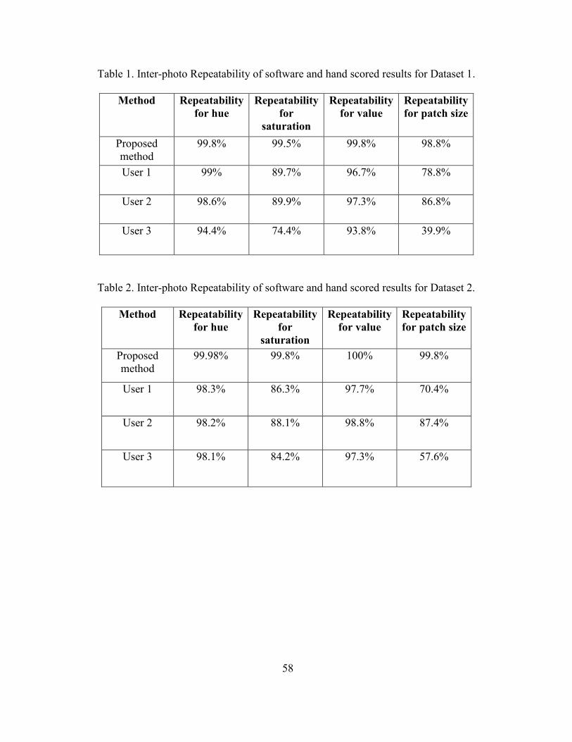
58

Table 1. Inter-photo Repeatability of software and hand scored results for Dataset 1.

Method Repeatability

for hue

Repeatability

for

saturation

Repeatability

for value

Repeatability

for patch size

Proposed

method

99.8% 99.5% 99.8% 98.8%

User 1 99% 89.7% 96.7% 78.8%

User 2 98.6% 89.9% 97.3% 86.8%

User 3 94.4% 74.4% 93.8% 39.9%

Table 2. Inter-photo Repeatability of software and hand scored results for Dataset 2.


for hue

Repeatability

for

saturation

Repeatability

for value

Repeatability

for patch size

Proposed

method

99.98% 99.8% 100% 99.8%

User 1 98.3% 86.3% 97.7% 70.4%

User 2 98.2% 88.1% 98.8% 87.4%

User 3 98.1% 84.2% 97.3% 57.6%

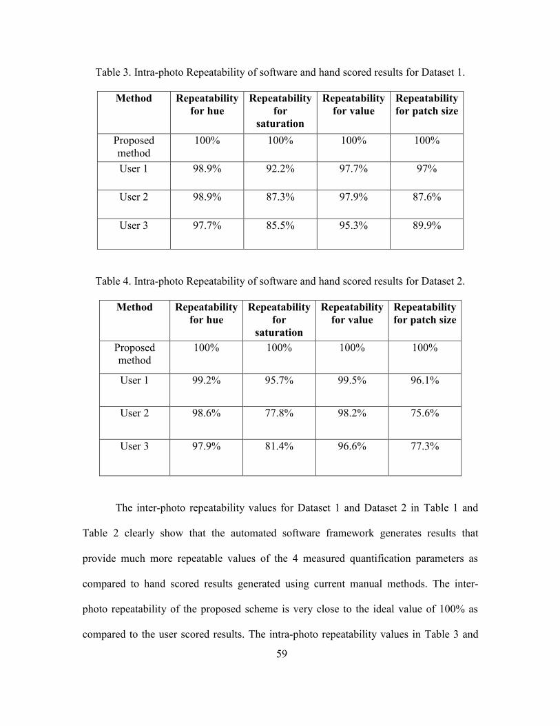
59

Table 3. Intra-photo Repeatability of software and hand scored results for Dataset 1.


for hue

Repeatability

for

saturation

Repeatability

for value

Repeatability

for patch size

Proposed

method

100% 100% 100% 100%

User 1 98.9% 92.2% 97.7% 97%

User 2 98.9% 87.3% 97.9% 87.6%

User 3 97.7% 85.5% 95.3% 89.9%

Table 4. Intra-photo Repeatability of software and hand scored results for Dataset 2.


for hue

Repeatability

for

saturation

Repeatability

for value

Repeatability

for patch size

Proposed

method

100% 100% 100% 100%

User 1 99.2% 95.7% 99.5% 96.1%

User 2 98.6% 77.8% 98.2% 75.6%

User 3 97.9% 81.4% 96.6% 77.3%

The inter-photo repeatability values for Dataset 1 and Dataset 2 in Table 1 and

Table 2 clearly show that the automated software framework generates results that

provide much more repeatable values of the 4 measured quantification parameters as

compared to hand scored results generated using current manual methods. The inter-

photo repeatability of the proposed scheme is very close to the ideal value of 100% as

compared to the user scored results. The intra-photo repeatability values in Table 3 and

60

Table 4 show that the proposed method produces results that are identical for pairs of

identical images scored a few days apart. However, the user scored results for the same

pairs of identical images are not identical and this proves that the proposed method

produces much more repeatable results as compared to manual scoring methods.

5.4 Correlation Analysis of the Proposed Framework

The correlation analysis of the proposed framework is evaluated by computing the linear

correlation coefficient between results generated using proposed method and user-scored

results. The Pearson’s correlation coefficient is computed for quantifying the correlation

between the results generated using the proposed framework and user scored results. The

correlation coefficient between two random variables X and Y with means 𝜇𝑥 , 𝜇𝑦 and

variances 𝜎𝑥2 , 𝜎𝑦

2 respectively is given as,

𝜌(𝑋, 𝑌) =𝐸[(𝑋−𝜇𝑥)(𝑌−𝜇𝑦)]

𝜎𝑋𝜎𝑌 (52)

Hand segmented ROIs are generated for all 33 specimens in dataset 1 and 25 specimens

in dataset 2 by three different users as explained in 5.2. The correlation coefficient is

computed between proposed method and user 1, proposed method and user 2 and

proposed method and user 3, for all the four measured quantification parameters. The

correlation coefficients for dataset 1 and dataset 2 are shown in Table 5 and Table 6

respectively. The proposed framework shows very strong correlation with all user scored

results for the measured hue and value of the region of interest. The correlation between

the proposed automated method and the manual scoring method is weaker for the

measured saturation and patch size. This is due to the low inter-photo and intra-photo

repeatability of manual scored results for saturation and patch size as compared to the

61

Table 5. Linear correlation of proposed method with user scored results for Dataset 1.

Correlation Pair Hue Saturation Value Patch size

Proposed method to

user 1

0.9975 0.9063 0.9729 0.7768

Proposed method to

user 2

0.9711 0.8160 0.9807 0.4832

Proposed method to

user 3

0.9863 0.8364 0.9738 0.7023

User 1 to User 2 0.9699 0.8863 0.9816 0.6976

User 2 to User 3 0.9844 0.9024 0.9759 0.7120

User 1 to User 3 0.9864 0.8911 0.9807 0.8242

Table 6. Linear correlation of proposed method with user scored results for Dataset 2.

Correlation Pair Hue Saturation Value Patch size

Proposed method to

user 1

0.9887 0.8335 0.9668 0.8124

Proposed method to

user 2

0.9845 0.8227 0.9710 0.8301

Proposed method to

user 3

0.9903 0.8969 0.9744 0.8764

User 1 to User 2 0.9870 0.8840 0.9861 0.8747

User 2 to User 3 0.9898 0.9120 0.9858 0.9292

User 1 to User 3 0.9864 0.8795 0.9893 0.8543

62

(a) Correlation Coefficient 𝜌 = 0.9975

(b) Correlation Coefficient 𝜌 = 0.9711

(c) Correlation Coefficient 𝜌 = 0.9863

Fig. 25 Correlation scatter plots for measured hue of Dataset 1. (a) Relation

between proposed method and user 1. (b) Relation between proposed method and

user 2. (c) Relation between proposed method and user 3.

63




Fig.26 Correlation scatter plots for measured saturation of Dataset 1. (a) Relation

between proposed method and user 1. (b) Relation between proposed method and user 2.

(c) Relation between proposed method and user 3.

64




Fig. 27 Correlation scatter plots for measured value of Dataset 1. (a) Relation between


Relation between proposed method and user 3.

65




Fig. 28 Correlation scatter plots for measured patch size of Dataset 1. (a) Relation



66




Fig. 29 Correlation scatter plots for measured hue of Dataset 2. (a) Relation between



67




Fig. 30 Correlation scatter plots for measured saturation of Dataset 2. (a) Relation



68




Fig. 31 Correlation scatter plots for measured value of Dataset 2. (a) Relation between



69




Fig. 32 Correlation scatter plots for measured patch size of Dataset 2. (a) Relation



70

Fig. 33 Performance relationship between results generated using proposed scheme and

user scored results for dataset 1 and dataset 2.

repeatability of the automated method for the same. The low repeatability of measured

saturation is directly related to the low repeatability of measured patch size. Human

observers tend to include pixels in the ROI based on the difference between the perceived

color, brightness of a small region of pixels and its neighborhood in the image. There can

be significant variation in the way the human visual system identifies such a region of

pixels and its corresponding neighborhood depending on the image zoom during ROI

selection and this results in the variation observed in the measured patch size. The

variance of the saturation value of all pixels in the plumage region of the birds is much

0

0.1

0.2

0.3

0.4

0.5

0.6

0.7

0.8

0.9

1

Rump Hue RumpSaturation

RumpBrightness

Rump Patchsize

Breast Hue BreastSaturation

BreastBrightness

BreastPatch size

Pea

rso

n's

Co

rrel

atio

n C

oef

fici

ent

Performance relation between proposed method and user scored results

Proposed method to user 1 Proposed method to user 2 Proposed method to user 3

71

higher than the variance of the hue and value of the same pixels. As a result, a variation

in the measured patch size produces a much higher variation in the average saturation

measurement for the ROI as compared to the average hue and value measurement for the

same ROI. This reduces the repeatability of the measured saturation. On the other hand,

the proposed framework relies on local pixel level color and brightness differences to

identify the pixels in the ROI. This helps to reduce variation in the patch size of the

selected ROI and in turn improves the repeatability of hue, saturation and value

measurements.

Figs. 25-28 illustrate the relation between the proposed method and user scored

results of images in dataset 1, for all the four measured parameters. Similarly, Figs. 29-32

illustrate the relation between the proposed method and user scored results of images in

dataset 2, for all the four measured parameters. The performance relationship of the

proposed method with user scored results for dataset 1 and dataset 2 is shown in Fig. 33.

72

CHAPTER 6

CONCLUSION

This thesis implements a framework for automated quantification of animal coloration in

digital images. This work contributes to the field of image segmentation in general and to

the area of animal color quantification in particular. This chapter summarizes the

contributions of this thesis and proposes several directions for future research.

6.1 Contributions

In this thesis, a novel method that automatically segments and quantifies an animal color

region of interest in digital images, is developed and implemented. The contributions of

the thesis can be summarized as follows:

A novel perceptual-based approach for the segmentation of animal coloration and its

quantification using variables such as hue, saturation, brightness, patch size etc., in

digital images with slowly varying background colors is presented.

A novel perceptual-based Saturation-Brightness quantization is implemented for the

removal of perceptually insignificant colors and only retaining the bright colors of

interest

This work develops a framework for segmenting the animal color region of interest

by coarsely segmenting the image into foreground and background regions using

dominant color quantization and then refining the foreground using skin pixel

classification and a perceptual based Saturation-Brightness quantization scheme.

73

The proposed framework produces much more repeatable and accurate results as

compared to existing user-driven manual methods and also avoids the inter-observer

error produced during manual scoring of results.

The proposed method is much faster than existing user-based manual approaches and

also produces results that are consistent with hand scored results. It takes an observer

around 2-3 minutes to select an ROI using the manual methods while the software

produces the result in less than 20 sec.

6.2 Future Research Directions

Possible enhancements to the proposed approach and future directions of research include

the following:

Incorporate robust background subtraction – The current work focuses on using

images that have slowly varying background color. The work needs to be extended in

the future to be able to process images acquired out in the field with variation in

background illumination and presence of texture and other structures in background.

Use of non-human color spaces – The color space used for color quantification in the

proposed framework (H, S, V) is human based. Since, humans cannot perceive colors

that lie outside the visible spectrum, human-based color spaces may not be a good

choice for color quantification in certain applications. Although, humans are unable

to perceive colors that lie in the UV spectrum, many animal species, especially birds

have the ability to perceive colors in the UV spectrum. Since color signals are used by

animals to attract prey, produce camouflage to hide from predators or attract mates

74

for breeding, it is important to incorporate non-human animal-based color spaces of

the target receivers to understand the role of animal colors in these applications.

Improve the algorithm to incorporate some sort of prior information about the

specimen in the image to be able to segment complex color traits such as those found

in chameleons, butterflies etc. and extend the scope of the algorithm to even perform

recognition or classification based on such traits.

Implement an adaptive Saturation-Brightness quantization scheme that assigns a pixel

to the ROI by considering not only its own Saturation and Brightness values but also

of the neighboring pixels.

The proposed method is currently being used to extract color traits of birds, butterflies

and reptiles. This work can be extended to target more difficult challenges like

disease detection in animal species and population/species classification.

75

REFERENCES

[1] E. H. Paxton, "The Utility of Plumage Coloration for Taxonomic and Ecological

Studies," The Open Ornithology Journal, vol. 2, pp. 17-23., 2009.

[2] M. Stevens, C. A. Parraga, I. C. Cuthill, J. C. Partridge and T. S. Troscianko, "Using

Digital Photography to Study Animal Coloration," Biological Journal of the Linnean

Society, vol. 90, pp. 211-237, 2007.

[3] K. J. McGraw, "Mechanics of melanin-based coloration," in Hill GE, McGraw KJ,

Eds. Bird Coloration: Mechanisms and Measurements, vol. 1, Cambridge: Harvard

University Press, 2006, pp. 243-294.

[4] K. J. McGraw, "Mechanics of Carotenoid-based coloration," in Hill GE, McGraw KJ,

Eds. Bird Coloration: Mechanisms and Measurements, vol. 1, Cambridge: Harvard

University Press, 2006, pp. 177-242.

[5] G. E. Hill, "Ornamental traits as indicators of environmental health," Bioscience, vol.

45, pp. 25-31, 1995.

[6] N. Johnson and R. Jones, "A new species of tody-tyrant (Tyrannidae: Poecilotriccus)

from northern Peru," Auk, vol. 118, pp. 334-41, 2001.

[7] M. Stevens, M. C. Stoddard and J. P. Higham, "Studying primate color: towards

visual system-dependent methods," International Journal of Primatology, vol. 30, no. 6,

pp. 893-917., 2009

[8] F. B. Bercovitch, "Testicular function and scrotal colouration in patas monkeys.,"

Journal of Zoology, vol. 239, pp. 93-100, 1996.

[9] L. A. Isbell, "Seasonal and social correlates of changes in hair, skin, and scrotal

condition in vervet monkeys (Cercopithecus aethiops) of Amboseli National Park,

Kenya," American Journal of Primatology, vol. 36, pp. 61-70, 1995.

[10] J. M. Setchell and A. F. Dixson, "Changes in the secondary sexual adornments of

male Mandrills (Mandrillus sphinx) are associated with gain and loss of alpha status,"

Hormones and Behavior, vol. 39, pp. 177-184, 2001

[11] S. Andersson and M. Prager, "Quantifying colors," in In G. E. Hill & K. J. McGraw

(Eds.),Bird coloration vol. I: Mechanisms & measurements, Cambridge, MA, Harvard

University Press, 2006, pp. 41–89.

[12] W. S and R. C., Computational colour science using MATLAB, Chichester: John

Wiley & Sons, 2004.

76

[13] A. Alsam and R. Lenz, "Calibrating color cameras using metameric blacks," JOSA A,

vol. 24, no. 1, pp. 11-17., 2007.

[14] P. Ferns and S. Hinsley, "Immaculate tits: head plumage pattern as an indicator of

quality in birds," Animal Behaviour, vol. 67, pp. 261-272., 2004.

[15] M. Vanacova and P. Adamik, "Feather ornaments are dynamic traits in the Great Tit

Parus major," Ibis, vol. 153, pp. 357-362, 2011.

[16] B. Matysiokova and V. Remes, "Egg yolk antioxidant deposition as a function of

parentalornamentation, age, and environment in great tits.," Journal of Avian Biology,

vol. 43, pp. 387-396, 2010.

[17] K. J.McGraw and G. E. Hill., "Plumage brightness and breeding-season dominance

in the house finch: a negatively correlated handicap?," Condor, vol. 102, pp. 457-462.,

2000.

[18] K. J. McGraw, A. M. Stoehr, P. M. Nolan and G. E. Hill, "Plumage redness predicts

breeding onset and reproductive success in the house finch: a validation of Darwin's

theory," J. Avian Biol., vol. 32, pp. 90-94, 2001.

[19] K. J. McGraw and G. E. Hill, "Carotenoid-based ornamentation and status signaling

in the house finch," Behavioral Ecology, vol. 11, no. 5, pp. 520-527, 2000.

[20] K. J. McGraw, P. M. Nolan, A. M. Stoehr and G. E. Hill., "Intersexual differences in

age-specific parental effort in the house finch.," Etologia, vol. 9, pp. 35-41, 2001.

[21] K. J. McGraw, W. Medina-Jerez and H. Adams., "Carotenoid-based plumage

coloration and aggression during molt in male house finches.," Behaviour, vol. 144, pp.

165-178, 2007.

[22] L. Busin, N. Vandenbroucke and L. Macaire, ""Color spaces and image

segmentation."," Advances in imaging and electron physics, vol. 151, pp. 65-168, 2008.

[23] R. W. Hunt, "Measuring Colour," in Measuring Colour, 3rd ed., England: Fountain

Press, 1998, pp. 39-57.

[24] J. Schanda, Colorimetry, Wiley-Interscience., 2009.

[25] A. R. Smith, "Color gamut transform pairs," in Proceedings of ACM SIGGRAPH,

vol. 12, pp. 12-19, 1978.

[26] A. Dempster, N. Laird and D. Rubin, "Maximum Likelihood from Incomplete Data

via the EMAlgorithm," Journal of the Royal Statistical, vol. 39, no. 1, pp. 1-38, 1977.

77

[27] R. Duda, P. Hart and D. Stork, Pattern Classification, New York: John Wiley &

Sons, 2001.

[28] A. C. Bovik, Handbook of image and video processing, Elsevier, 2010.

[29] A. Said and L. J.Karam, "Cell Migration Analysis using a Statistical Level-Set

Segmentation on a Wavelet-Based Structure Tensor Feature Space," 7th IEEE

International Symposium on Signal Processing and Information Technology (ISSPIT),

pp. 473-478, 2007.

[30] T. J. Bergman and J. C. Beehner, "A simple method for measuring colour in wild

animals: validation and use on chest patch colour in geladas (Theropithecus gelada).,"

Biological Journal of the Linnean Society, vol. 94, no. 2, pp. 231-240, 2008.

[31] D. Kendal, C. E. Hauser, G. E. Garrard, S. Jellinek, K. M. Giljohann and a. et,

"Quantifying Plant Colour and Colour Difference as Perceived by Humans Using Digital

Images.," PLoS ONE, vol. 8(8): e72296., 2013.

[32] Adobe Photoshop. [Online] Available: http://www.photoshop.com/products

[33] GIMP 2.8. [Online] Available: http://www.gimp.org/

[34] ImageJ [Online] Available: http://rsb.info.nih.gov/ij/

[35] R. Montgomerie, "Analyzing colors," in Hill GE, McGraw KJ, Eds. Bird Coloration:

Mechanisms and Measurements, vol. 1, Cambridge: Harvard University Press, 2006, pp.

90-147.

[36] Y. Vortman, "Measuring animal coloration in nature: A protocol for scoring colors

based on the RGB model and Adigital photography software tool". [Online] Available:

http://ibis.tau.ac.il/twiki/bin/view/Zoology/Lotem/YoniVortman

[37] D. Comaniciu and P. Meer, "Robust analysis of feature spaces: Color image

segmentation," in IEEE CVPR, pp. 750-755, 1997.

[38] R. Szeliski, "Segmentation," in Computer Vision:Algorithms and Applications, New

York, NY,, Springer-Verlag New York, Inc., 2010, pp. 289-296.

[39] P. Heckbert, "Color image quantization for frame buffer display," ACM SIGGRAPH

Computer Graphics, vol. 16, no. 3, pp. 297-307, July 1982.

[40] D. Arthur and S. Vassilvitskii, "k-means++: The advantages of careful seeding," in

Proceedings of the eighteenth annual ACM-SIAM Symposium on Discrete Algorithms,

pp. 1027-1035, 2007.

http://www.photoshop.com/products

http://www.gimp.org/

http://rsb.info.nih.gov/ij/

http://ibis.tau.ac.il/twiki/bin/view/Zoology/Lotem/YoniVortman

78

[41] W. Y. Ma, Y. Deng and B. S. Manjunath, "Tools for texture/color based search of

images," in Proc. SPIE Human Vision and Electronic Imaging II,vol. 3016, pp. 496-507,

1997.

[42] A. Mojsilovic, J. Kovacevic, J. Hu, R. J. Safranek and S. K. Ganapathy, "Matching

and retrieval based on the vocabulary and grammar of color patterns," IEEE Transactions

of Image Processing, vol. 1, no. 1, pp. 38–54, Jan. 2000.

[43] Y. Deng, B. S. Manjunath, C. Kenney, M. S. Moore and H. Shin, "An efficient color

representation for image retrieval," IEEE Transactions of Image Processing, vol. 10, no.

1, pp. 140–147, Jan. 2001.

[44] A. Mojsilovic, J. Hu and E. Soljanin, "Extraction of perceptually important colors

and similarity measurement for image matching, retrieval, and analysis," IEEE

Transactions of Image Processing, vol. 11, no. 11, pp. 1238–1248, Nov. 2002.

[45] Y. Linde, A. Buzo and R. M. Gray, "An algorithm for vector quantizer design,"

IEEE Transactions on Communications, vol. 28, no. 1, pp. 84–95, Jan. 1980..

[46] J. Smith and S. F. Chang, "Single color extraction and image query," in IEEE Int.

Conf. Image Processing,, vol. 3, pp. 528-531, 1995.

[47] J.-C. Terrillon, M. David and S. Akamatsu, "Automatic detection of human faces in

natural scene images by use of a skin color model and of invariant moments," in Proc. of

the Third International Conference on Automatic Face and Gesture Recognition, pp.

112-117, 1998.

[48] J. Yang, W. Lu and A. Waibel, "Skin-Color Modeling and Adaptation.," in

Proceedings of the Third Asian Conference on Computer Vision, vol. II, pp. 687-694,

1998.

[49] J.-C. Terrillon, M. N. Shirazi, H. Fukamachi and S. Akamatsu, "Comparative

performance of different skin chrominance models and chrominance spaces for the

automatic detection of human faces in color images," in Fourth IEEE International

Conference on Automatic Face and Gesture Recognition, pp. 54-61, 2000.

[50] T. S. Jebara and A. Pentland, "Parameterized structure from motion for 3D adaptive

feedback tracking of faces," in IEEE CVPR, pp. 144-150, 1997.

[51] S. J. McKenna, S. Gong and Y. Raja, "Modeling facial color and identity with

Gaussian mixtures," Pattern Recognition, vol. 31, no. 12, pp. 1883-1892, 1998.

[52] H. Akaike, "A new look at the statistical model identification," IEEE Transactions

on Automatic Control, vol. 19, no. 6, pp. 716–723, 1974.

79

[53] Lemke-Rust, Kerstin and a. C. Paar, "Gaussian mixture models for higher-order side

channel analysis," in Cryptographic Hardware and Embedded Systems, Berlin

Heidelberg, pp. 14-27, 2007.

[54] J. Canny, "A computational approach to edge detection," IEEE Transactions on

Pattern Analysis and Machine Intelligence, vol. 8, no. 6, pp. 679-698, 1986.

[55] R. R. Sokal and F. J. Rohlf, Biometry: the principles and practice of statistics in

biological research, New York: W. H. Freeman and Co, 1981.

[56] C. M. Lessells and P. T. Boag, "Unrepeatable Repeatabilities: A Common Mistake,"

The Auk, vol. 104, no. 1, pp. 116-121, 1987.

80

APPENDIX A

ANOVA TABLES AND VARIANCE COMPONENT TABLES

81

Table A1. Inter-photo repeatability ANOVA table for measured hue in Dataset 1.

Source of

variation

Degrees of

freedom

Sum of

squares

Mean squares F ratio

Among groups

for software

32 3517.907 109.935

807.676 Within groups

for software

33 4.4917 0.13611

Total variation

for software

65 3522.398 54.1907

Among groups

for user 1

32 3400.399 109.69


for user 1

33 17.2527 0.5391

Total variation

for user 1

65 3417.652 54.2484

Among groups

for user 2

33 3574.499 108.318

137.959 Within group

for user 2

32 26.695 0.7851

Total variation

for user 2

65 3601.194 53.749

Among groups

for user 3

33 3079.166 96.2239


for user 3

32 91.994 2.78771

Total variation

for user 3

65 3171.16 48.7871

82

Table A2. Inter-photo repeatability variance components for measured hue in Dataset 1.

Component Component variance % of Total

Among groups for

software

54.8992 99.8

Within groups for

software

0.1361 0.2473

Total variance for

software

55.0353 100

Among groups for

user 1

54.5755 99.02

Within groups for

user 1

0.5391 0.9782

Total variance for

user 1

55.1147 100

Among groups for

user 2

53.7665 98.6

Within groups for

user 2

0.7851 1.4

Total variance for

user 2

54.5516 100

Among groups for

user 3

46.7181 94.4

Within groups for

user 3

2.7877 5.6

Total variance for

user 3

49.5058 100

83

Table A3. Inter-photo repeatability ANOVA table for measured saturation in Dataset 1.

Source of

variation

Degrees of

freedom

Sum of

squares

Mean

squares

F ratio

Among groups

for software

32 1147.982 35.8744


for software

33 3.1685 0.0960

Total variation

for software

65 1151.151 17.71

Among groups

for user 1

32 2345.693 75.6675

18.4060

Within groups

for user 1

33 131.5525 4.1110

Total variation

for user 1

65 2477.246 39.3214

Among groups

for user 2

32 2318.172 70.2476


for user 2

33 127.216 3.7416

Total variation

for user 2

65 2445.389 36.4983

Among groups

for user 3

32 2820.612 88.1441


for user 3

33 427.755 12.9623

Total variation

for user 3

65 3248.368 49.9749

84

Table A4. Inter-photo repeatability variance components of measured saturation in

Dataset 1.


Among groups for

software

17.8892 99.5

Within groups for

software

0.0960 0.5339

Total variance for

software

17.9852 100

Among groups for

user 1

35.7782 89.7

Within groups for

user 1

4.1110 10.3

Total variance for

user 1

39.8892 100

Among groups for

user 2

33.2529 89.9

Within groups for

user 2

3.7416 10.1

Total variance for

user 2

36.9946 100

Among groups for

user 3

37.5909 74.4

Within groups for

user 3

12.9622 25.6

Total variance for

user 3

50.5532 100

85

Table A5. Inter-photo repeatability ANOVA table for measured value of Dataset 1.

Source of

variation

Degrees of

freedom

Sum of

squares


Among groups

for software

32 2563.382 80.1057


for software

33 2.3951 0.0725

Total variation

for software

65 2565.77 39.4735

Among groups

for user 1

32 4012.874 129.448


for user 1

33 69.5800 2.1743

Total variation

for user 1

65 4082.454 64.8009

Among groups

for user 2

32 3789.824 114.843


for user 2

33 53.237 1.565

Total variation

for user 2

65 3842.061 57.359

Among groups

for user 3

32 4462.188 139.443

31.1564

Within group

for user 3

33 147.6947 4.4756

Total variation

for user 3

65 4609.883 70.9213

86

Table A6. Inter-photo repeatability variance components for measured value in Dataset 1.


Among groups for

software

40.0165 99.8

Within groups for

software

0.0725 0.181

Total variance for

software

40.0891 100

Among groups for

user 1

67.4838 96.7

Within groups for

user 1

4.4755 3.3

Total variance for

user 1

71.9594 100

Among groups for

user 2

56.6386 97.3

Within groups for

user 2

1.5657 2.7

Total variance for

user 2

58.2044 100

Among groups for

user 3

63.6365 93.8

Within groups for

user 3

2.1743 6.2

Total variance for

user 3

65.8109 100

87

Table A7. Inter-photo repeatability ANOVA table for measured patch size in Dataset 1.

Source of

variation

Degrees of

freedom

Sum of

squares


Among groups

for software

32 1.22e+11 3.82e+9


for software

33 7.496e+8 2.27e+7

Total variation

for software

65 1.23e+11 1.89e+9

Among groups

for user 1

32 1.47e+11 4.76e+9


for user 1

33 1.81e+11 5.65e+8

Total variation

for user 1

65 1.66e+11 2.63e+9

Among groups

for user 2

32 7.26e+11 2.2e+10


for user 2

33 5.3e+10 1.56e+9

Total variation

for user 2

65 7.79e+11 1.2e+10

Among groups

for user 3

32 3.49e+11 1.1e+10

2.3250 Within group

for user 3

33 1.55e+11 4.69e+9

Total variation

for user 3

65 5.04e+11 7.76e+9

88

Table A8. Inter-photo repeatability variance components for measured patch size in

Dataset 1.


Among groups for

software

1.90e+9 98.8

Within groups for

software

2.27e+9 1.2

Total variance for

software

1.92e+9 100

Among groups for

user 1

3.10e+9 78.8

Within groups for

user 1

4.69e+9 21.2

Total variance for

user 1

7.80e+9 100

Among groups for

user 2

1.02e+10 86.8

Within groups for

user 2

1.55e+9 13.2

Total variance for

user 2

1.17e+10 100

Among groups for

user 3

2.09e+9 39.9

Within groups for

user 3

5.64e+8 60.1

Total variance for

user 3

2.66e+9 100

89

Table A9. Inter-photo repeatability ANOVA table for the measured hue in Dataset 2.

Source of

variation

Degrees of

freedom

Sum of

squares


Among groups

for software

24 2889.127 120.38


for software

25 0.2411 0.00965

Total variation

for software

49 2889.368 58.9667

Among groups

for user 1

24 3155.518 131.48


for user 1

25 28.6918 1.1476

Total variation

for user 1

49 3184.21 64.9839

Among groups

for user 2

24 3263.93 135.997


for user 2

25 30.3741 1.2149

Total variation

for user 2

49 3294.313 67.2309

Among groups

for user 3

24 3203.294 133.471


for user 3

25 32.8104 1.3124

Total variation

for user 3

49 3236.104 66.0429

90

Table A10. Inter-photo repeatability variance components for measured hue in Dataset 2.


Among groups for

software

60.1853 99.98

Within groups for

software

0.0096 0.02

Total variance for

software

60.1949 100

Among groups for

user 1

65.1661 98.3

Within groups for

user 1

1.1476 1.7

Total variance for

user 1

66.3137 100

Among groups for

user 2

67.3912 98.2

Within groups for

user 2

1.2149 1.8

Total variance for

user 2

68.6062 100

Among groups for

user 3

66.0790 98.1

Within groups for

user 3

1.3124 1.9

Total variance for

user 3

67.3914 100

91

Table A11. Inter-photo repeatability ANOVA table for measured saturation in Dataset 2.

Source of

variation

Degrees of

freedom

Sum of

squares


Among groups

for software

24 617.085 25.7119


for software

25 0.6163 0.02465

Total variation

for software

49 617.70 12.6062

Among groups

for user 1

24 1228.33 51.1804


for user 1

25 93.9608 3.7584

Total variation

for user 1

49 1322.291 26.9855

Among groups

for user 2

24 1434.365 59.7652


for user 2

25 94.6345 3.7853

Total variation

for user 2

49 1528.99 31.2041

Among groups

for user 3

24 1214.123 50.5884


for user 3

25 108.7534 4.3501

Total variation

for user 3

49 1322.876 26.9975

92

Table A12. Inter-photo repeatability variance components for measured saturation in

Dataset 2.


Among groups for

software

12.8436 99.8

Within groups for

software

0.0246 0.2

Total variance for

software

12.8682 100

Among groups for

user 1

23.7109 86.3

Within groups for

user 1

3.7584 13.7

Total variance for

user 1

27.4694 100

Among groups for

user 2

27.9899 88.1

Within groups for

user 2

3.7853 11.9

Total variance for

user 2

31.7752 100

Among groups for

user 3

23.1191 84.2

Within groups for

user 3

4.3501 15.8

Total variance for

user 3

27.4692 100

93

Table A13. Inter-photo repeatability ANOVA table for measured value in Dataset 2.

Source of

variation

Degrees of

freedom

Sum of

squares


Among groups

for software

24 1509.457 62.8941

87790 Within groups

for software

25 0.0179 0.0007

Total variation

for software

49 1509.475 30.8056

Among groups

for user 1

24 2291.522 95.4801


for user 1

25 27.2327 1.0893

Total variation

for user 1

49 2318.755 47.3215

Among groups

for user 2

24 2364.833 98.5347


for user 2

25 15.401 0.6160

Total variation

for user 2

49 2380.234 48.5762

Among groups

for user 3

24 2250.799 93.7833


for user 3

25 32.3718 1.2948

Total variation

for user 3

49 2283.17 46.5953

94

Table A14. Inter-photo repeatability variance components for measured value in

Dataset 2.


Among groups for

software

31.4466 100

Within groups for

software

0.0007 0.0023

Total variance for

software

31.4473 100

Among groups for

user 1

47.1953 97.7

Within groups for

user 1

1.0893 2.3

Total variance for

user 1

48.2846 100

Among groups for

user 2

48.9593 98.8

Within groups for

user 2

0.6160 1.2

Total variance for

user 2

49.5753 100

Among groups for

user 3

46.2442 97.3

Within groups for

user 3

1.2948 2.7

Total variance for

user 3

47.5390 100

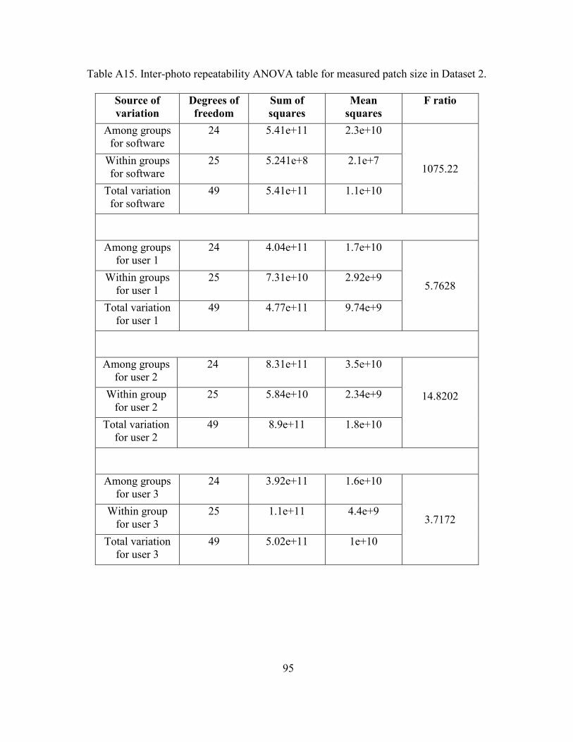
95

Table A15. Inter-photo repeatability ANOVA table for measured patch size in Dataset 2.

Source of

variation

Degrees of

freedom

Sum of

squares

Mean

squares

F ratio

Among groups

for software

24 5.41e+11 2.3e+10


for software

25 5.241e+8 2.1e+7

Total variation

for software

49 5.41e+11 1.1e+10

Among groups

for user 1

24 4.04e+11 1.7e+10


for user 1

25 7.31e+10 2.92e+9

Total variation

for user 1

49 4.77e+11 9.74e+9

Among groups

for user 2

24 8.31e+11 3.5e+10


for user 2

25 5.84e+10 2.34e+9

Total variation

for user 2

49 8.9e+11 1.8e+10

Among groups

for user 3

24 3.92e+11 1.6e+10

3.7172 Within group

for user 3

25 1.1e+11 4.4e+9

Total variation

for user 3

49 5.02e+11 1e+10

96

Table A16. Inter-photo repeatability variance components for measured patch size in

Dataset 2.


Among groups for

software

1.126e+10 99.8

Within groups for

software

2.09e+7 0.2

Total variance for

software

1.12e+10 100

Among groups for

user 1

6.96e+9 70.4

Within groups for

user 1

2.93e+9 29.6

Total variance for

user 1

9.88e+9 100

Among groups for

user 2

1.61e+10 87.4

Within groups for

user 2

2.33e+9 12.6

Total variance for

user 2

1.84e+10 100

Among groups for

user 3

5.97e+9 57.6

Within groups for

user 3

4.39e+9 42.4

Total variance for

user 3

1.03e+10 100

automated animal coloration quantification in digital ... · automated animal coloration...

Documents