auto-extraction of modelica code from finite element analysis or measurement data · ·...

Auto-Extraction of Modelica Code from Finite Element Analysis or

Measurement Data

The-Quan Pham1, Alfred Kamusella

2, Holger Neubert

2

1 OptiY e.K., Aschaffenburg Germany, e-mail: [email protected]

2 Technische Universität Dresden, Institute of Electromechanical and Electronic Design

Abstract

This paper presents a new approach to extract Mod-

elica codes from finite element analysis or measure-

ment data automatically. The finite element model or

the real system on the test bench is adaptively sam-

pled while applying the Gaussian process with a few

number of model calculations or measurement

points. Based on these support points, a meta- or

surrogate model of the system is built. Thus, Modeli-

ca codes can be generated automatically. These al-

gorithms are implemented in the multidisciplinary

design software OptiY®. Its application is demon-

strated on the example of an electromagnetic actua-

tor.

Keywords: Gaussian Process; Kriging; Surrogate

Modeling; Meta Modeling

1 Introduction

The manual modeling of technical systems with net-

work elements is a challenging and time-consuming

process. Considerable experience and knowledge on

the working principles is necessary. Commercial

software systems such as Dymola, Matlab/Simulink,

SimulationX, etc. provide ready-to-use model libra-

ries for this approach. However, they do not support

the elaboration of an adequate network structure. In

order to achieve a sufficient accuracy of the models,

an expensive parameter identification has to be per-

formed frequently. This can be achieved by compar-

ing the simulation results with those from experi-

mental investigations and then adjusting the network

parameters.

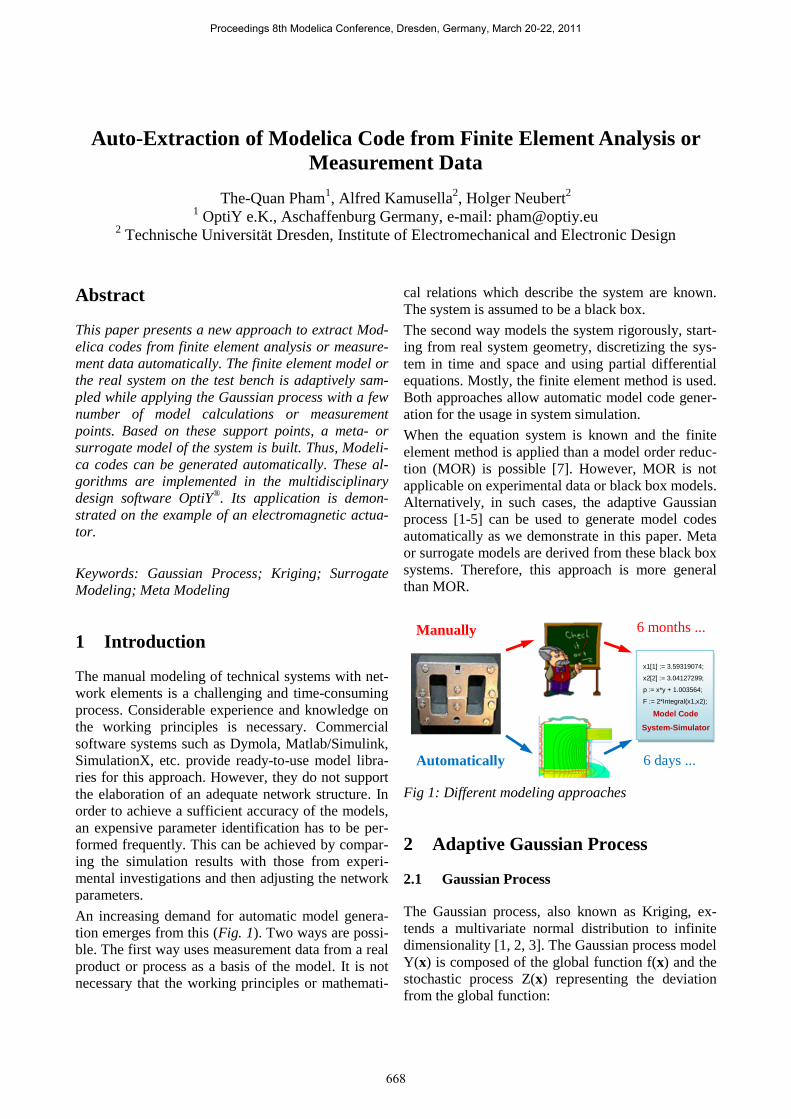
An increasing demand for automatic model genera-

tion emerges from this (Fig. 1). Two ways are possi-

ble. The first way uses measurement data from a real

product or process as a basis of the model. It is not

necessary that the working principles or mathemati-

cal relations which describe the system are known.

The system is assumed to be a black box.

The second way models the system rigorously, start-

ing from real system geometry, discretizing the sys-

tem in time and space and using partial differential

equations. Mostly, the finite element method is used.

Both approaches allow automatic model code gener-

ation for the usage in system simulation.

When the equation system is known and the finite

element method is applied than a model order reduc-

tion (MOR) is possible [7]. However, MOR is not

applicable on experimental data or black box models.

Alternatively, in such cases, the adaptive Gaussian

process [1-5] can be used to generate model codes

automatically as we demonstrate in this paper. Meta

or surrogate models are derived from these black box

systems. Therefore, this approach is more general

than MOR.

Fig 1: Different modeling approaches

2 Adaptive Gaussian Process

2.1 Gaussian Process

The Gaussian process, also known as Kriging, ex-

tends a multivariate normal distribution to infinite

dimensionality [1, 2, 3]. The Gaussian process model

Y(x) is composed of the global function f(x) and the

stochastic process Z(x) representing the deviation

from the global function:

x1[1] := 3.59319074;

x2[2] := 3.04127299;

p := x*y + 1.003564;

F := 2*Integral(x1,x2);

Model Code

System-Simulator

Manually 6 months ...

Automatically 6 days ...

Proceedings 8th Modelica Conference, Dresden, Germany, March 20-22, 2011

668

)()()(1

xxx ZfYp

i

ii

.

f(x) is the polynomial regression function of any or-

der, β are the unknown regression coefficients, and

Z(x) is a stationary stochastic process having mean

zero, variance σ2 and correlation function R(•). x is a

m-dimensional vector of input parameters.

It is assumed, that the training data or support points

consist of the simulation or measurement data at the

input set x1, x2, ..., xn and that y(x0) is the predicted

vector. The Gaussian process model implies the

points Y0 = Y(x0) and Yn = [Y(x1), ... Y(xn)]T having

the multivariate normal distribution:

R

r

rβ

F

f

Y

T

z

T

nnN

Y0

0

20

1

0 1, .

f0 = f(x0) is the (p, 1)-vector of regression function

for Y(x0). F = [fi(xi)] is the (n, p)-matrix of regres-

sion functions for the training data or support points.

r0 = [R(x0, x1), ..., R(x0, xn)]T is the (n, 1)-vector of

correlation functions of Yn with Y(x0), and R = R(xi,

xj) is the (n, n)-matrix of correlation functions among

Yn.

Therefore, the best linear unbiased predictor for

Y(x0) is the mean value of the multivariate normal

distribution. It represents the response surface, also

known as meta- or surrogate model, of the real sys-

tem:

)()( 1

000 FβYRrβfx nTTY

.

The uncertainty of the predicted value is characte-

rized by the variance of the multivariate normal dis-

tribution:

)()()(1 0

1

0

11

0

1

00

1

0

22rRFfFRFrRFfrRr

TTTTT

z .

2.2 Correlation Function

The correlation function is the crucial ingredient in

the Gaussian process predictor because it contains

assumptions about the function to be predicted. It

interpolates between support points in which its val-

ue smoothly changes between 0 and 1.

Several stationary correlation functions have been

investigated to approximate a lot of real functions or

systems [1]:

Gamma exponential

m

i

iwR1

2121 exp),( xxxx

Matérn class

2121

121

22

2)(

1),(

xxxxxx KR

Rational quadratic

2

21

2

21 1),(xx

xxw

R .

w, λ and α are hyper-parameters, which have to be

identified using optimization methods in order to

maximize the likelihood function of the multivariate

normal distribution. In some cases, the Gamma-

exponential correlation function is either exponential

(γ=1) or square exponential (γ=2). For the Matérn

class, the correlation functions with ν=3/2 and ν=5/2

are frequently used.

2.3 Adaptive Gaussian Process

With the variance σ2 of the multivariate normal dis-

tribution, the confidence interval (3σ) of the response

surface is available at any point. Thus, it is possible

to measure the accuracy of the meta model. Besides

the variance, the expected improvement (EI) has

been introduced as a second factor for meta model

evaluation purposes [4]. EI is defined as a potential

improvement which is achieved by investigating the

input parameter x:

YYYYYYEI

minminmin .

Φ(•) and (•) are commulative distribution functions

and probability density function of the normalized

normal distribution. A third evaluation factor is the

statistical low bounding (SLB) [5]:

kYSLB

with k =1,3,5...

Based on these three factors, the accuracy of the me-

ta model can be improved by using additional sup-

port points, which are suggested by the optimization

procedures to:

maximize EI,

maximize 3σ and

minimize SLB.

Meta modeling is an adaptive process, which in-

volves several loops of the Gaussian process. Start-

ing from the initial sampling points, the response

surface of the modeled system is built. Based on this

response surface, additional support points are sug-

gested and make possible that the new response sur-

face is rebuilt more accurately. The process comes to

an end either if a predetermined number of support

points is computed or if a specified value of maxi-


669

mum EI is achieved. The necessary number of sup-

port points for a specific accuracy of the surrogate

model depends on:

the number of input parameters x,

the correlation between input parameters and

the degree of nonlinearity of the surrogate

model.

The adaptive Gaussian process is very efficient for

meta modeling. It requires less support points when

compared with other design of experiment (DoE)

methods in order to achieve a comparable accuracy.

3 Code-Extraction with OptiY®

For system modeling purposes, commercial software

systems for CAD/CAE, FEA, CFD, electronic circuit

simulation, electro-magnetics, etc. are available. It is

better to use tailored programs for the different com-

ponents of a complex model. The advantages are:

easy usage and quick handling of the soft-

ware,

availability of expert knowledge,

detailed and accurate component behavior

modeling,

small number of model parameters, which

have to be identified.

For the system simulation, different component

models created by different software programs have

to be coupled. In general, this is difficult to arrange.

System models contain component models having a

large number of degrees of freedom. This results a

high computing effort for system simulation. Using

surrogate models in form of Modelica codes instead

of the underlaying component models reduces com-

putation time and cost drastically. Such fast system

models allow robust design optimization (RDO),

e. g. design for six sigma, and reliability based de-

sign optimization (RBDO) which both require a

large number of runs of system models.

The multitude of software tools normally used for

component modeling makes automatic computation

of the meta models desirable. The multidisciplinary

design software OptiY® supports the automatic gen-

eration of meta models in form of Modelica code

used in system models (Fig. 2) [7]. This software

provides generic and direct interfaces to many com-

mercial software systems for CAD, FEA, electronic

circuit simulation, CFD, multi body simulation, in-

house codes etc. Furthermore, user can easy self-

integrate external CAD/CAE-software for ease of

use later with a predefined user element and script

template using Visual Basic or C# based on the NET.

Framework® technology.

Fig 2: Auto-extraction of Modelica code with OptiY

The numerical algorithms of the adaptive Gaussian

process presented in last section are also imple-

mented in OptiY. For this reason an easy and quick-

to-use connection to external component models is

supported. Combined with the adaptive Gaussian

process, this allows the automatic extraction of Mod-

elica codes from external models or data.

With other implemented numerical algorithms in

OptiY, following valuable possibilities are also

available for the design process:

Sensitivity Study

Probabilistic Analysis

Reliability Analysis

Robustness Evaluation

Six Sigma Design

Robust Design

Design Optimization

Data Mining

Parameter Identification

4 Electromagnetic Actuator

We use a Braille printer with an electromagnetic ac-

tuator in order to demonstrate the system simulation

with surrogate models [8] (Fig. 3).

In the first step, the system model of the printer con-

sists only of network elements which are taken from

the model library of SimulationX [9]. The resulting

network schematic is shown in Fig. 4, left side. The

OptiY®

Modelica Code

CAD

FEM

CFD

Measurement Data

Electronics

Optics

Electro-Magnetics

Multi-Body-Dynamic

Multi-Physics


670

model computes the dynamic behavior of the actua-

tor.

Fig. 3: Braille printer with electromagnetic actua-

tor; 1 back iron, 2 coil, 3 return spring, 4 armature,

5 guiding air gap, 6 needle, 7 paper sheet, 8 die, 9

yoke, 10 working air gap

In the second step, we replace the magnetic network

elements by a finite element model applying the

software FEMM [10] (Fig 4).

Fig 4: System model of the Braille printer; network

model (left) and finite-element model (right) of the

magnetic parts of the actuator

OptiY controls the FEMM tool, provides the input

vector of the sampling points and collects the simula-

tion results. After the simulation is finished, the sur-

rogate model of the magnetic part of the actuator is

computed by the adaptive Gaussian process and ex-

ported as Modelica code. All magnetic network ele-

ments (yellow block in Fig. 4) are replaced by surro-

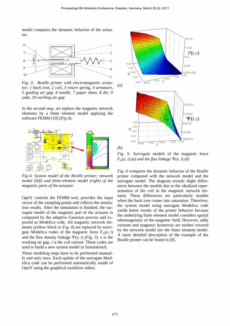
gate Modelica codes of the magnetic force Fm(x, i)

and the flux density linkage (x, i) (Fig. 5). x is the

working air gap, i is the coil current. These codes are

used to build a new system model in SimulationX.

These modeling steps have to be performed manual-

ly and only once. Each update of the surrogate Mod-

elica code can be performed automatically inside of

OptiY using the graphical workflow editor.

(a)

(b)

Fig. 5: Surrogate models of the magnetic force

Fm(x, i) (a) and the flux linkage (x, i) (b)

Fig. 6 compares the dynamic behavior of the Braille

printer computed with the network model and the

surrogate model. The diagram reveals slight differ-

ences between the models due to the idealized repre-

sentation of the coil in the magnetic network ele-

ment. These differences are particularly notable

when the back iron comes into saturation. Therefore,

the system model using surrogate Modelica code

yields better results of the printer behavior because

the underlying finite element model considers spatial

inhomogeneity of the magnetic field. However, eddy

currents and magnetic hysteresis are neither covered

by the network model nor the finite element model.

A more detailed description of the example of the

Braille printer can be found in [8].


671

Fig. 6: Dynamic behavior of the Braille printer si-

mulated by a network model (dashed) and a surro-

gate model (solid); x - printer needle displacement, i

- coil current, F - magnetic force

5 Conclusions

Modeling technical systems with network elements

is an adequate approach, however, challenging and

time-consuming if performed manually. The adap-

tive Gaussian process is an approach that allows an

efficient and automatic generation of precise compo-

nent models for system modeling. It requires only

few support points of the black box system. With

additional support points, the accuracy of the com-

puted meta model can be improved step by step if

necessary. The mathematical meta model can be

written as Modelica code. The algorithms which are

needed for this procedure are implemented in the

multidisciplinary design software OptiY®. It pro-

vides generic and direct interfaces to many specia-

lized commercial CAD/CAE-software tools and also

in-house codes. Within, user can easily create fast

surrogate models and export them as Modelica code

automatically.

The study case shows that the meta modeling process

is very fast and useful. The amount of identified pa-

rameters is smaller in comparison to the network

model. The system behavior is more accurate. The

application of a Braille printer with an electromag-

netic actuator has been demonstrated. Simulation

results of a network model and a surrogate model

have been compared. The use of fast meta models

allows computationally intensive optimization and

test procedures, e. g. robust design optimization.

References

[1] Rasmussen C. E., Williams C. K. I.: Gaus-

sian Process for Machine Learning. MIT

Press 2006.

[2] Santner, T. J., Williams, B. J., Notz, W. I.:

The Design and Analysis of Computer Expe-

riment. Springer New York 2003

[3] Sacks J., Welch W. J., Mitchell T. J., Wynn

H. P.: Design and Analysis of Computer Ex-

periments. Statistical Science 4, pp. 409-435,

1989

[4] Jones, R. D.: A Taxonomy of Global Optimi-

zation Methods Based on Response Surfaces.

Journal of Global Optimization 21: 345-383,

2001

[5] Xiong, Y., Chen, W, and Tsui, K.: A New

Variable Fidelity Optimization Framework

Based on Model Fusion and Objective-

Oriented Sequential Sampling. ASME Jour-

nal of Mechanical Design , 130 (11), 2008

[6] Antuolas, A. C.: Approximation of Large-

Scale Dynamical Systems. SIAM 2005

[7] OptiY Software and Documentation.

www.optiy.eu

[8] http://www.optiyummy.de/index.php/Softwa

re:_FEM_-_Tutorial_-_Magnetfeld,

see Kennfeld-Export als Modelica-Code

[9] SimulationX Software and Documentation.

www.iti.de

[10] FEMM Software and Documentation.

www.femm.info


672

auto-extraction of modelica code from finite element analysis or measurement data · ·...

Documents