author(s) swett, jorge eduardo. title monterey, california
TRANSCRIPT

Calhoun: The NPS Institutional ArchiveDSpace Repository
Theses and Dissertations 1. Thesis and Dissertation Collection, all items
1973
Performance analysis of digital radiometers.
Swett, Jorge Eduardo.Monterey, California. Naval Postgraduate School
http://hdl.handle.net/10945/16741
Downloaded from NPS Archive: Calhoun

PERFORMANCE ANALYSIS OF
DIGITAL RADIOMETERS
Jorge Eduardo Swett

Library
Naval Postgraduate SchoolMonterey, California 93940

JRADUATE SC
Monterey, California
ii U U L
THESISPERFORMANCE ANALYSIS
OF. DIGITAL RADIOMETERS
by
Jorge Eduardo Swett
Thesis Advisor: J.E. Ohlson
March 1973
T 154583
Ajap^oved Ion. pubLLc itl&aAe.; dL&&ubLi£ion unLlmltcd.


Performance Analysisof
Digital Radiometers
by
Jorge Eduardo SwettLieutenant, Chilean Navy
B.S., United States Naval Academy, 1966Ingeniero Naval Electronico, Academia
Politecnica Naval, Chile, 1969
* Submitted in partial fulfillment of therequirements for the degree of
ELECTRICAL ENGINEER
from the
NAVAL POSTGRADUATE SCHOOLMarch 1973

5 5

ary .
'
l Postgraduate SchoolMonterey, California 93940
ABSTRACT
This work investigates the effects of digital processing
in radiometers. It deals mainly with two digital versions
of a total power radiometer. The first consists of RF,
Mixer and IP sections followed by an analog to digital
converter. All further processing is done in a digital
computer. The second version consists of RF, Mixer and IF
sections followed by a square lav; detector, RC filter and
analog to digital converter. From this point on the pro-
cessing is done by a digital computer. A figure of merit
is defined based on the performance of an analog total power
radiometer. Exact results are obtained for the figure of
merit of the first digital version. For the second, an
approximate solution is obtained. The effects of saturation
and finite step size of the quantizer were taken into con-
sideration for the above results. The performance of digital
balanced-Dicke and noise-adding radiometers is investigated
using the above results. The effects of digital filtering
on the performance of a radiometer is considered.


TABLE OF CONTENTS
I. INTRODUCTION 8
II. PERFORMANCE FIGURE OF A RADIOMETER.DEGRADATION FACTOR 12
III. DEGRADATION FACTOR CALCULATION WITH NOQUANTIZER 17
A. IF SAMPLING 17
1. Ideal Filter 20
2. Single Tuned Filter 23
3. Gaussian Filter 25
4. Butterworth Filter 26
B. RC FILTERING THEN SAMPLING 28
IV. TRANSFER CHARACTERISTICS OF A QUANTIZER WITH AZERO MEAN GAUSSIAN INPUT PROCESS 31
A. QUANTIZER ALONE 32
B. QUANTIZER FOLLOWED BY SQUARE LAW DETECTOR - 46
V. DEGRADATION FACTOR CALCULATION WITH AQUANTIZER 50
A. IF SAMPLING 50
1. Exact Solution 50
a. Ideal Filter 56
b. Single Tuned Filter 62
c. Gaussian Filter 68
d. Butterworth Filter 74
2. An Approximation 54
B. RC FILTERING AND THEN SAMPLING 84
1. First Approximation 84


2. Second Approximation 102
VI. DYNAMIC RANGE AND LINEARITY OF A DIGITALRADIOMETER — 104
A. IF SAMPLING 104
B. RC FILTERING AND THEN SAMPLING 107
VII. APPLICATION TO SWITCHING RADIOMETERS 110
A. DICKE 110
B. NAR 113
VIII. DIGITAL FILTERING 119
IX. CONCLUSION 126
APPENDIX 128
LIST OF REFERENCES 15*1
INITIAL DISTRIBUTION LIST 156
FORM DD 1473 157


LIST OF FIGURES
FIGURE
1 ANALOG TOTAL POWER RADIOMETER 9
2 IF SAMPLING DIGITAL TOTAL POWER RADIOMETER 10
3 RC FILTERING AND SAMPLING DIGITAL TOTAL POWERRADIOMETER 11
4 OUTPUT CHARACTERISTICS OF TYPICAL TOTAL POWERRADIOMETER 12
5 IDEAL BANDPASS FILTER CHARACTERISTICS 21
6 BLOCK DIAGRAM OF QUANTIZER AND QUANTIZERFOLLOWED BY SQUARE LAW DETECTOR 32
7 QUANTIZER CHARACTERISTICS 33
8 through 14 TRANSFER CHARACTERISTICS OFQUANTIZER 39
15 TRANSFER CHARACTERISTICS OF QUANTIZER FOLLOWEDBY SQUARE LAW DETECTOR 49
16 CHANNEL OF IF SAMPLING TOTAL POWER RADIOMETER — 51
17 EXPECTED VALUE OF OUTPUT OF IF SAMPLING CASE 55
18 through 2 3 DEGRADATION FACTOR FOR IF SAMPLINGCASE USING AN IDEAL BANDPASS INPUTFILTER 56
.24 through 29 DEGRADATION FACTOR FOR IF SAMPLINGCASE USING A SINGLE TUNED INPUTFILTER 62
30 through 35 DEGRADATION FACTOR FOR IF SAMPLINGCASE USING A GAUSSIAN INPUT FILTER — 68
36 through 41 DEGRADATION FACTOR FOR IF SAMPLINGCASE USING A BUTTERWORTH INPUTFILTER OF ORDER TWO 74
42 CHANNEL OF IF SAMPLING TOTAL POWER RADIOMETERS - 80
43 COMPARISON OF DEGRADATION FACTOR FOR IF SAMPLINGCASE BETWEEN EXACT SOLUTION AND APPROXIMATION — 83


44 QUANTIZER CHARACTERISTICS 85
45 CHANNEL OP RC FILTERING AND SAMPLING CASE 86
46 through 51 DEGRADATION FACTOR FOR RC FILTERINGAND SAMPLING. ZERO OFFSET 92
52 TRANSFER CHARACTERISTICS OF QUANTIZER WITHOFFSET 98
53 DEGRADATION FACTOR FOR RC FILTERING ANDSAMPLING. QUANTIZER WITH OFFSET 99
54 COMPARISON OF DEGRADATION FACTOR FOR RCFILTERING AND SAMPLING FOR THE TWOAPPROXIMATIONS USED 100
55 EXPECTED VALUE OF OUTPUT OF IF SAMPLING CASE 106
56 EXPECTED VALUE OF OUTPUT OF RC FILTERING ANDSAMPLING CASE 108
57 DIGITAL BALANCED DICKE RADIOMETER, IF SAMPLINGCASE 111
58 DIGITAL BALANCED DICKE RADIOMETER, RC FILTERINGAND SAMPLING CASE 112
59 DIGITAL NAR, IF SAMPLING CASE 115
60 DIGITAL NAR, RC FILTERING AND SAMPLING CASE 116
61 EXPECTED VALUE OF OUTPUT, DIGITAL NAR, IFSAMPLING CASE 118
62 BLOCK DIAGRAM OF DIGITAL FILTER 120


ACKNOWLEDGMENT
The author wishes to thank Professor John E. Ohlson of
the Department of Electrical Engineering of the U.S. Naval
Postgraduate School for his constant support, valuable
ideas, comments and corrections made throughout this thesis.
To my wife and children, for their understanding and
patience,, I am deeply grateful.


I. INTRODUCTION
A radiometer is basically a highly sensitive and stable
noise receiver. The principle of operation lies in the fact
that any object at temperatures above absolute zero radiates
energy in the form of electromagnetic waves. Until some
years ago, radiometers were used mainly as radio telescope
receivers and constituted the main tool of Radio Astronomy
[Ref. 1]. Lately, their use has expanded to many other
areas. The measurement of atmospheric temperature [Refs. 2
and 3] » detection of air turbulence in the Troposphere
[Ref. 4], airborne mapping [Ref. 5], the measurement of
absolute radiation from a projectile flow field [Ref. 6],
and passive detection [Ref. 7] can be cited as examples.
The type of processing involved in a radiometer is
especially .fitted to digital methods. A number of insti-
tutions have integrated the radiometer with the digital
computer in their applications. The purpose of this work
is to investigate the effects of this integration, and to
provide guidelines to the design of digital radiometers.
The main body of the investigation will deal with two
digital versions of a total power radiometer (TPR) shown in
Figure 1. The first one (Figure 2) consists of RF, Mixer,
and IF sections, followed by an Analog to Digital Converter
(ADC) section. All further processing is done in a digital
computer. The second one (Figure 3) consists of RF, Mixer,


and IF sections followed by a square law detector, a low
pass filter, and an ADC. From that point on, the processing
is done by a digital computer.
The main difference of the two cases is the location of
the ADC. The second version (Figure 3) is presently being
used and its main advantages over the first version (Figure
2) is that it requires a much lower sampling rate.
The results obtained for a total power digital radiometer
can be used to determine performance of other types of
radiometers. Performance of digital Dicke and noise-adding
radiometers will be considered.
V
X VRF}MIX, IP
H.(n
SQUARE LAW
"DETECTOR
iNTE^fcATOR-
z
FIGURE 1


M
*©*JH
Of*-
- «?
u «>
\
4" CT+-
1
CJ aQ P< «=c
iiM
X X
CO 3 tf
S UJa, Lj
J- h3 J 5 -J
o — o -_i u-
4J
_J u-
o
r>a, 3 Aa-
CM
W
oMft
3°
c
1
10


H
«3
a+-
t>
>•
on
C3MPC
11


II. PERFORMANCE FIGURE OF A RADIOMETER.DEGRADATION FACTOR
By definition, the sensitivity, or minimum detectable
temperature, of a radiometer is taken as that change in
operating temperature T that causes a change in the expected
value of the output equal to one standard deviation of the
output [Ref. 1]. Refer to Figure 4. It shows the expected
value and the standard deviation of the output voltage as
functions of temperature for a typical radiometer.
outpo t"
vol+ctoe.
ECU
FIGURE 4
12


Prom Figure 4, It follows that (to first order)
aeci] . ffim AT (1)op
where E[«] = Expected value of [•], and T is operating
temperature. But by definition
AE[I] = a-= dE[I]
T dTop op
(2)
Therefore
AT = "IdELIJ
dT 'op
(3)
A performance figure can be defined as,
ATTop
T
dE[I]dT
op
(4)
It can be shown [Ref. 1] that for an analog total power
radiometer (Figure 1), using the fact that the inverse of
the integration time is much smaller than the bandwidth of
the RF, Mixer, IF filter, that
E[I] = TkT / |H (f)| df°P _co" ' °
(5)
aT
2= 2xk
2T
2/ |H
Q(f)|
4df (6)
13


where
t = Integration time
H (f) = Band-pass filter (RF,Mix,IF) frequencyresponse
k = Boltzmann 1 s constant
Substituting into (4)
\ AT _ 1
Top (B
et)^2
(7)
where
( / |Ho(f)|
2df)
2
be = —°=
;< 8 >
/ |H (f)|? df
The performance figure of the analog TPR, (7), will be
used as a basis for evaluating the performance of a digital
TPR. Hence, the Degradation Factor can be defined as
-, _ Performance figure of Digital RadiometerPerformance figure of Analog Radiometer
Intuitively, F should be equal or greater than one since
as the sampling rate of the ADC goes to infinity and the
step size of the quantizer goes to zero, both digital
radiometers are reduced to an analog TPR.
Some comments are appropriate at this point. First,
(5) and (6) show that for analog radiometers E[I] and a_
1A


are linear functions of temperature and go through the
origin. Hence equation (4) reduces to
iT- ^T (9)T
op
The addition of a quantizer, due to saturation, makes
E[I] and a_ nonlinear with respect to temperature, and the
performance figure is thus temperature dependent. There-
fore (4) must be used instead of the better-known (7).
Secondly, the parameter T in equation (4) is not a
convenient choice, since for a given T , different gain
settings of the RP, Mixer, IP filter will change the
performance of the radiometer. Referring to Figures 2 and
3 it is easily shown that
T = a aY2
(Figure 2) (10)c
T= 3 az
(Figure 3) (11)
where a and 3 are proportionality constants. Using the
2parameters a or a as appropriate, instead of T, norma-c
lizes the problem of gain setting out of the performance
figure
.
15


Then, for the radiometer of Figure 2
AT
^opdE[IJ
da. aX
2at T
c op
(12)
and for the radiometer of Figure 3
ATrop
dELl]da„ a 7 at T ,
Z op
(13)
16


III. DEGRADATION FACTOR CALCULATION WITH NO QUANTIZER
An ADC performs two basic operations on a signal. One
is sampling, and the other is amplitude quantization. In
this chapter the effects of sampling alone are considered.
Hence it is assumed that each sample can be represented
without any error.
\
A. IF SAMPLING
Refer to Figure 2. Assume that at the antenna white
gaussian noise is present with double-sided power spectral
density No/2 watts/hertz. Then X(t) is a Narrow Band
Gaussian Process with known power spectral density, and
can be represented as
X(t) = X (t)cos27rf t - X (t)sin2TTf t (14)C OS o
where X (t) and X (t) are baseband Gaussian processes ands c
f is the IF center frequency of the radiometer. It can
be shown [Ref. 8] that if X(t), X (t) and X (t) are to bec s
wide sense stationary, then
RX (y) = R
X (y) (15)c s
RY (y) = RY (u)cos2Trf y + RY v (y)sin2TTf u (16)c s c
17


where R (y) is the autocorrelation function of the process
X(t) and RY y. (y) is the crosscorrelation function of thes c
'processes X (t) and X (t).c s
Furthermore if H (f) is symmetrical about f (this iso o
the only case considered in this work) , then
Rx x (y) = (17)c s
and RY (y) is given byXc
RY (y) = 2 / S (f)cos[2Tr(f-f )y]df (18)Ac
x °
and Sv (f), the power spectral density of X (t), is theA Cc
Fourier Transform of equation (18).
Physically, for the case of interest (i.e. X(t), X (t)
and X (t) wide sense stationary, and H (f) symmetrical abouts o
f ), S„ (f) is Just twice the low pass version of SY (f).O A AC
Referring to Figure 2, the low pass filters filter out the
double-frequency terms coming out of the multipliers. Then
I = I±
+ I2
(19)
I-, - } 2 X„2(kA) (20)
x n k=1 c
since X (kA) = q (kA) and
18


*o = h l X2(kA) (21)
d n k=l s
since X (kA) = q (kA).s s
Using the fact that for Gaussian random variables
E[X1X2X3X4
] = E[X1X2]EOC
3X
i|]+E[X
1X3]E[X
2X4]+E[X
1X
i|]E[X
2X3
]
(22)
and expanding the double summation, it follows that
2oY
^n-1
aT
d= —2_ + 1 e (1-£)RY
d(kA) (23)
Xl
n nk=l
n Xc
and
EC^] = ax
2(24)
For the random variable I?
the same results are obtained
since Rx
(u) = Rx (y)
c s
Then
E[II]= 2aY2
(25)2 X
c
and
aj 2 = oI
2+ a
I
2+ 2E[I
1I2
] - 2E[I1]E[I
2]
1 2"
(26)
19


Expanding E[I I? ] and using the fact that R„ „ (y) = 0,
c s
the last two terms of (26) cancel out.
Using equations (25) and (26) in (12) it follows that
op naY k=l c
c
or
1 (^-)2
= | + -^ ^ (1 - |)Rx2(kA) (28)
op xax
k=l c
c
where
t = nA (29)
The degradation factor squared is
5 2B„A n-1 . . 9F^ = B A + —\ I (1 - £A)R ^(kA) (30)
ax
k=l c
c
RY (y) is a function of H (f), therefore (30) will be usedAc
°
with four different frequency characteristics.
1. Ideal Bandpass Filter
Refer to Figure 5
N B sirnrBy
V (p> = -^m— (31)
20


© H.Cf)
I
© i
2
Ho
2
,' >
J.
4
© S^(l)
*f2
B2
FIGURE 5
21
and
V = NQ
B (32)
Substituting (3D and (32) into (30)
F2
= Bp A + 2BT,A
nE
1
(l-^) ^llLI^ (33)E Ek=l
T(irkAB)
2
But
BE
= B = W (34)
where BE
is the equivalent bandwidth from (8) and W is the
half- power bandwidth.
Then (33) can be rewritten as
t?2 TTA , otta v sin irkW 2(WA) r ksin TrkW r->c\F = WA + 2WA E 5- - 'l — p— (35)
k=l (TrkWA)^TW
k=l (TTkWA)
Since t>>A, it can be shown that the third term of (35)
is much smaller than the second and thus can be ignored.
Letting A approach zero (sampling infinitely fast), (35)
becomes
P2 . 2W ) sinfuWt
dt (36)(irWt)
and then since t is large, the integral's upper limit can
be replaced by infinity, and the integral reduces to one,
giving the correct result.
22


Actually, by including the third term as A goes to zero,
P will be slightly less than one. The reason for this is
that in calculating the performance figure of an analog TPR
in (7) the fact that - << B was used to get (5) and (6).
Had this fact not been used, as A approached zero, F would
approach one exactly.
P will be plotted as a function of WA. Hence, for this
case the Nyquist sampling rate (twice the highest frequency)
corresponds to WA = 1 .
The analysis done in this chapter is Just a special case
of the analysis that will be done in Chapter V, hence all
results will be plotted in the figures of that chapter. The
results obtained from (35) for an ideal bandpass filter are
plotted in Figures 18 through 23. It is of interest to note
that for W less than one (sampling faster than the Nyquist
rate), F is exactly equal to one, an intuitively satisfying
result.
2. Single Tuned Filter
For a Single Tuned Filter
l
Ho(f)
l
2 = h^-;* b-r "7)
where W is the half power bandwidth and W is much less than
f . It follows thato
Sx(f) =
-f |Ho(f)|
2(38)
23


and
and
and
NSY (f) = Vt (39)X
c 1 + M§)2
From (39) > using the Inverse Fourier Transform
N W ...|
Rx (y) = -g— e
—n-Wlvl(40)
Top
T Tk-1
Equation (.41) can be put in closed form by letting
A = e"27rWA
(42)
Using the fact that [Ref. 9]
k=l -
1 " A
V kAk = A-nAn + (n-l)An+1
(1|i()
k=l (l-AT
and after some tedius but straightforward manipulations, it
follows that
2
(fM2
=f-
(coth ttWA) - |p (cosech2
irWA)(l - e"27rWx
) (45)op
and
F2
= AB„(coth ttWA) - (ABe)fnnaa,
v, 2 „taWi q -2ttWTv ,,.,-xE id (cosech ttWA)(1 - e ) (^b;
2TBE
24


It can be shown that the equivalent bandwidth of a
single tuned fulter is [Ref. 1]
BE
= ttW (47)
where W is the half-power bandwidth. Furthermore, since
t>>A, the second term is negligible with respect to the
first, hence
F2 = 7rwA(coth ttWA) (48)
To compare with the analog case, let A go to zero.
Then P would become one, which is the correct result.
Figures 24 through 29 show the results obtained for this
filter.
3. Gaussian Filter
For a Gaussian Filter
, -v (£=£°) 2 v(£l£2.) 2
[Ho(f)]
2= e
W+ e
W(49)
where v = 4 In 2 = 2.773, W is the half-power bandwidth, and
W is much less than f .
o
It follows that
-v(§)2
SY ..(f) = N eW
(50)
and
Xc
V' °
-!l!(Wy) 2
Rx (y) = N W(J-)
J5
ev
(51)
25


Replacing equation (51) Into (30) and using the fact
that for this filter
BE= (2JL)Sl = 1.505 W (52)
it follows that
2n"1 kA "|(lTkWA)2
F^ = 1.505WA + 3-01WA E (1-^F) e (53)k=l
T
\
Using the same argument as before (A<<t), (53) becomes
n-1 -|(TTkWA)2
F^ = 1.505WA + 3.01W I e (54)k=l
To compare to the analog case let A approach zero. Then
(5^) becomes
P t -|(irkWA)2
F^ = 3-01W / e (55)
and since x is large, the integral's upper limit can be
replaced by infinity, and the integral reduces to one, as
it should. The numerical results are plotted in Figures 30
through 35.
.4. Butterworth Filter
The last filter to be considered is a Butterworth
Filter of order two. For this case
i + i6<-vr> l + iec-jfV
where W is the half-power bandwidth, and W is much less than f
26


Then
NSY (f) = 2—r-E (57)X
c 1 + 16(§)4
and
Rx (y) = -V e (2)^ cos(l±^ _J) (58)X
c2
(2)4
For this filter, it can be shown that
Bv = -^-^ ttW = 1.48W (59)E3
Substituting (58) and (59) into (30) it follows,
after some effort that
n—
1
hF2
= 1.48WA + 2.96WA Z e~k7r(2) 2WA
[1 + sintku^^WA]k=l
-- 2 '96(AW) 2 Vke^ (2^WA[l + sin(k,(2)^A] (60)
TW k=l
Again it can be argued that the third term is negligible,
therefore
n— 1 Js
F2
= 1.48WA + 2.96WA E e'k7T(2) 2WA
[1 + sin(k7r (2) 2̂WA) ] (61)k=l
Comparing to the analog case by letting A approach
zero, (6l) becomes
t hF2
= 2.96WA / e"7r(2)2Wt
[l + sin(TT(2)J'2Wt)]dt (62)
27


Since x is large, the integral's upper limit can be replaced
by infinity, and it reduces as it should to one.
The numerical results for this filter are plotted
in Figures 36 through 4l.
B. RC FILTERING AND THEN SAMPLING
Refer to Figure 3. This type of digital TPR was studied
by Ohlson [Ref. 10] for the case where no quantizer is
present. Only the results and its implications are presented
here.
It can be shown that
NE[Z] = g -f (63)
and
c 72
= g2 &) 2 l (64)
Z & v2
2BEtRC
where g is a system gain parameter, N is as defined on
page 17, and tRC is the time constant of the RC filter.
Also
E[I] = E[Z] (65)
and
crT2 = -|-+ 2
f E (1- ^-)[R7(kA)-E
2[Z]] (66)
1 n Tk=l T L
where R 7 (u) is the autocorrelation function of the process Z(t).
28


Substituting (65) and (66) into (13), we have
_ , kA
op E RC k=l
Defining
A = e~A/t RC (68)
and using equations (43) and (44) it can be shown that
\
(1 e-T/tRCw A A s2
P2 . A
cothA _ ^J )^t RC
CSCh2t RC
)
(69)<^RC ^RC ( T /t RC )
Equation (69) is of the same form as equation (47).
Note that in that case it was argued that the second termo
was negligible since tW was large (oh the order of 10 )
.
Here the same assumption can not be made since r— << Wfc RC
(i.e. the RC filter bandwidth is much smaller than the
bandwidth of the RF, Mixer, IP filter). The first term of
equation (69) reduces to one as A approaches zero. The
second term however, contributes negatively. Therefore F
can be less than one. The reason for this lies in the addi-
tion of an RC filter to the radiometer ^ which has the effect
of lengthening the integration time x. As A approaches zero,
a comparison is being made of two TPR, one with an RC filter
after the square law detector and the other without one.
The one with the RC filter will have greater sensitivity
(smaller AT) due to a longer effective integration time.
Therefore F can be less than one.
29


However, if the effects of sampling only are of interest
(not the effect of the addition of the RC filter), the
second term must be disregarded by assuming that T/t R „ = °°.
This implies that all the filtering is done by the integrator
and none by the RC filter.
As explained in part A of this chapter, the results are
presented in Chapter V. Refer to Figures 46 through 51.
In summary, the effects of an ideal ADC (i.e. no
saturation and step size equal to zero) was studied in this
chapter. Its main importance is the fact that it provides
a lower bound for the Degradation Factor and, that under
certain conditions, a correction can be added to these
results to account for the finite step size of the quantizer.
30

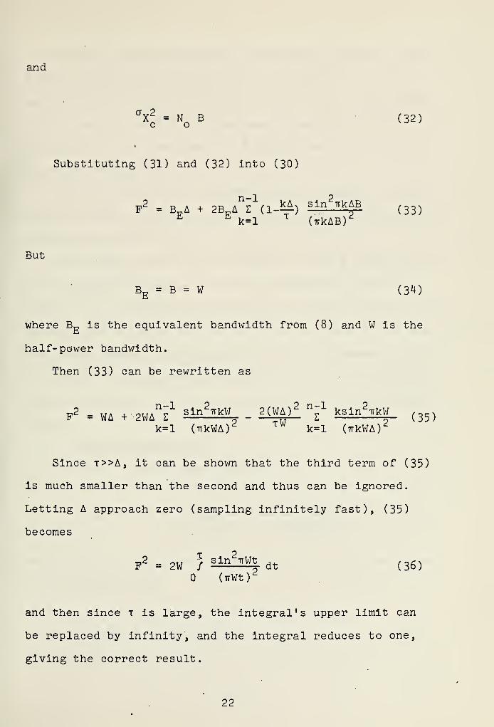
IV. TRANSFER CHARACTERISTICS OF A QUANTIZERWITH A ZERO MEAN GAUSSIAN INPUT PROCESS
In this chapter the effects of a quantizer on a zero
mean Gaussian input process are analyzed. Two cases are
investigated. Refer to Figure 6. It is desired to find
the autocorrelation function at point 2 given the auto-
correlation function of X(t) and the knowledge that it is
Gaussian and has zero mean. Several approaches have been
explored for the case of a quantizer alone. The one sug-
gested by Kellog [Ref.ll] was used since it can be easily
extended for the case of a quantizer followed by a square
law detector, and also the equations that it leads to are
In a form suitable for computer programming. Figure 7
shows two quantizers, one with even number of levels and
the other with odd number of levels.
Let N be the number of levels of the quantizer. Then
_ 2L(i - N/2)(?0)
*i n-1UU;
and
n = 2L[i - (N+l)/2] rrnqi N-1 w J
31


Ub)
X(k)
SQUPr &ELAWDETECTOR YCt)
FIGURE 6
A. QUANTIZER ALONE
The autocorrelation function of q(t) is
Rq(y) = E{Q[X(t)]Q[X(t+y]} (72)
Let
X(t) = ?. (73)
and
X(t+y) = 5, (74)
Then
00 00
Rq(y) = f f Q(? 1 )Q(c 2
)f(?1 ,C 2
;y)dC1dC
2(75)
_oo _oo
32


a._
oj- levels
-L *.-i—i-
%i- -i
'_
Xn_(
A
.
/l
^o
^.
VL
b._ Odd number
o^- levels
-L *v-t—t-
Sm
i
aX t)-\
T
1
%
s.
/•_
//
FIGURE 7
33 '.


where
_ (^-2pA C2-K
2
2)
(1-PX2
) 2ax2
f(C .,? 9 ;y) = - _ ^^ (76)1 2
a2
2-rr (l-p v2 )*
and
RY (y)PX " •i
xT0T-(77)
Noting that the dependence of R upon u is only via pv ,q a
the notation R„(P V ) will be used for brevity. Then (75)q A
becomes
N N X. X
1-1 j-1 x±_1
Xj^
(78)
Let
B1
= ?1/a
x (79)
32
= ?2/a
x(80)
then (78) can be written as
h i -(B1
2-2px e132+e2
2)
ay cty ?
N N p 2(1-0,-)Rq(px
) = 2 2 q1qJ/ / S . *
d3id32
(8l)1=1 j=1 X
i-1 Vl 2(1 -p 2 )^_ _ Aax ax
34


but
B l
2" 2f3 i e 2 p X
+ 32
2 = (B 2 " P X 3 1)2 + B
l2(1 " P X
)2 (82)
Therefore
rh2
~ 2 PXg l g 2+ g
2
2
,- (g
2 - p X gl
)
261
2
> Rq ,- L 5 J = 5— 5— (03;2(1 - p/) 2(1 - p/) 2
and (8lV becomes
p
Xi 2
X .
"(32"pX6l )
N N „ n ~ov 1 h /2 oye
2(l-p2
)
R (py) = Z E qlqj /A
2~Fe
/X X_
d |3 pd3.. (84)
q Xi-1 j=l X^ X^ C2Tr(l-p
x2)]'2
2 X
~°x~aX
Now "let
B2- p^
= a
^(l-px2)]"5
(85)
It follows that the second Integral can be written as
1 (erft V"* '"ft ] - erfC i^X^^ ]} (86)
2 I [2(1-Pv )V [2(1-PT2 )T 1
where
erf(a) = -4- / e"v dv (87)tt^
35


If a new function is defined as
N q. r X,/aY - py6, X. ,/o - p 8JL l ^ff -J—£ £Ji i . Pr.f r -iz±—£
—
JL± ] t (88)X X
j=l2
l [2(l-px2)]'2 [2(l-p
x2)]
then (84) can be written as
Xi 2
iN
«F-^
Rrt (py)
=' k z 3, / ^(pY ,e n ) e 2 d(3
n(89)
q X(2tt)^ i=l
1Xi_1
X X 1
2Dividing both sides of (89) by ay and substituting the
expressions for X. and q. , it is found that a new parameter
appears, namely aY/L . This parameter together with N and
Pxwill be the independent variables of (89). Note that with
the introduction of cry/L , the dynamic range of the quantizer,
L, is no longer an independent factor.
By letting
(90)
(91)
(92)
qi= qi
/L
X£ = X±/L
and- CT
i = ax/L
it follows that
\Vpx}
_ 1
^ (2ir)*
n q^
1=1 'X xi-i
V^'(p
x ,61
) e""2"
d61
(93)
and
36


N q»f
X'/a' - py6 nX! -,/a' - pi ^
•(PjcA) - 2 gX erfC J X M ] - erf [ J"1 X P ] (94)
It can be shown, following a similar procedure, that for
p„ equal to one, (93) becomes
Ra(l)
°a 1N qi 2 f
Xi/aX
Xi-l
/aX 1-S_ = J- . i z (
i.
)
2erf[ -L-£ ] - erf[ -^-^ ] (95)
ax2 a
x22
1=1 aX I (2)2
{2)h >
2This gives us a numerically so we can get the normalized
autocorrelation of q. Equations (93) through (95) allow the
computation of the autocorrelation function of the output of
a quantizer of N steps and saturation level L given that the
input is Gaussian, zero mean, and of known autocorrelation
function. The procedure would be as follows. First,
calculate a ' , X' and q' for the given quantizer and input
process. Second, find a value of p yfor a particular u
(Equation (76)). Third, form the function ^'(px ,B
1) for
the particular value of p„ determined in the second step.
Fourth, replace the function ^'(px ,B-.) into (93) and perform
the integration. This procedure will map one point of the
input autocorrelation function into one point of the output
autocorrelation function.
A program was written to solve (93) through (95) for the
case of symmetrical quantizers (See Appendix under Transfer
Characteristics of Odd level Quantizer, and Transfer Charac-
teristics of Even level Quantizer) and the results are
37


plotted in Figures 8 through 14 as a function of pv . TheRa (v)ordinate axis is a = p . In other words, for a given
q2 q
pY , p is obtained. The advantage of plotting it this waya q
is that the curves are independent of the input autocorrela-
tion function (as long as the input process is Gaussian and
zero mean).
In general, the curves are a function of tf-v/L (except for
the special case of N=2). Note that for N=2 the result is\
the well-known relationship [Ref. 7]
MPX ) pq A= =- arcsin p Y (96)
ad i\ A
q
It is of interest to note the behavior of these curves as
aY/L approaches extreme values. For a quantizer with odd
number of levels, as tfy/L gets very large, the quantizer will
appear as a hard limiter, hence the curves will approach that
of Figure 8. As ay/L approaches zero the quantizer will
appear as a three step quantizer (eventually it will become
an open circuit) and the curves will show a behavior similar
to those shown in Figure 9. For a quantizer with an even
number of levels, the behavior of the curves as ay/L becomes
large is also as described above. When cr /L approaches zero,
however, the quantizer will appear again as a hard limiter,
therefore the curves will approach that of Figure 8.
38


* N=2
nn
itCI /r j
1
1
f,
'W2 rjca JuU U-J 303
yrna
nfit
hi
n
k-scrle-4. 00e-01 units inch.
v-scrlp:----4.ooe:-oi units inch.
FIGURE 8
39


?*
N/--3
O1.5"-
""3H\
OX
Q.lol
/X 0.4 >
L
rjr ipi^ f.
-012 ^023 Juu ]Q4 jca
/ Sjf f JO
4?
wsY
a
ffj
CJi
K-SCRLE-4.00E-Q1 UNITS INCH.
V-SCRLE-4.00E-01 UNITS INCH.
FIGURE 9
no


K-5GRLE----4- OOE-01 UNITS INCH.
Y-SCRLE----4. OOE-01 UNITS INCH,
FIGURE 10
41


p* KJ = 5
o<->
<
O.Cp ///
/TV ;
~0.if
o-8 //
on
^ /-US
/? /&y /
Or.i
^* _>'/r
Py
t'012 -029 -cc^,
r
3CC 334 :c6
/J^ r r j
C71
/dY[J/ 11
C)
1
o1
rt-3CRLE----4.QQE-dl UNITS INCH,
Y-SCRLE=4.Q0E-01 UNITS INCH.
FIGURE 11
h2


f1 M-7
mn
o.c -0.4o.tf >V
^<^y
^V/ - l.Ss
\
LIt J P»
r(U2 -OSQ /T
'i iiz-i 023
-
A^ -fCl73
4//ef t i
1
rCl
K-3CRLE-4.00E-01 UNITS INCH.
^-SCRLE---4.Q0E-01 UNITS INCH.
FIGURE 12
^3


K-SCflLE=4.00E-01 UNITS INCH.
V-SCRLE----4.00E-01 UNITS INCH.
FIGURE 13
44


h N-17
CI
ok ^ = 0.2L
o.fc
OS./j7
/
n/l -1.5
JT-S
j
n
j/z
'itr
ft
an -UC9 -uC*^
yjr
IjV ]29
s ni
A^6/ Cl
exa
/&
K-SCRLE----4.00F-01 UNITS INCH.
Y-SCRLE=4. OOE-01 UNITS INCH,
FIGURE 14
45


B. QUANTIZER FOLLOWED BY A SQUARE LAW DETECTOR
The reason for analyzing this case will become apparent
in Chapter V. Refer to Figure 6 and observe that
Y(t) = q2(t) (97)
and
q(t) = Q[X(t)] (98)
R^y) = E[Y(t)Y(t+y)] (99)
Upon substituting (97) and (98) into (99) it follows
that
Ry(y) = E{Q2[X(t)]Q
2[X(t+y)]} (100)
Following a similar procedure as done for the previous case,
(100) becomes
— 2
Vfv) iN <M p °x
"3l
1uA
= —±-r- S (rr) / A(pY ,3 n) e~2~ dB, (101)
cx4
(2ir)* i=l ffX Xjj X X X
~3T
and
N q'r
X'/a' - p 6n X' -,/a' - pY^ACp-A ) - i E ftp{erf[
3 X2 V ] - erf[ 'J'1 X " P ]} ( 102
)
j-l°X C2(1-PX2)]^ [2(l-p
x2)]^ J
For PY=1 it can ^e shown that
ECY2] _ 1 ? ,
qix4 r- ,
Xi , ... Xj-i v
-i Mn ,v-5-TT
=? E Czt") [erf ( r ) - erf ( j- ) J (103)V d
1=1aX a
x(2)^ a
x(2)^
46


Xi> q i> °X>
and P Xwere deflned ln (90), (91), (92) and (77)
respectively.
A computer program was written for this case when the
quantizer Is symmetrical (See Appendix under "Transfer
Characteristics of Odd Quantizer Followed by a Square Law
Detector" and "Transfer Characteristics of Even Quantizer
Followed by a Square Law Detector"). The same comments as
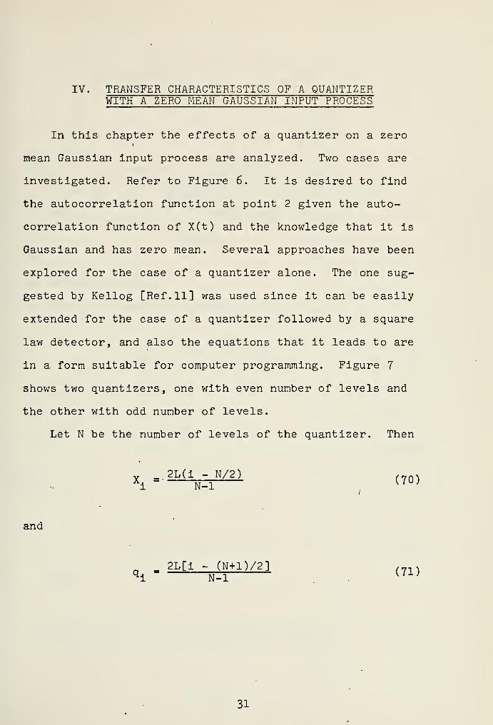
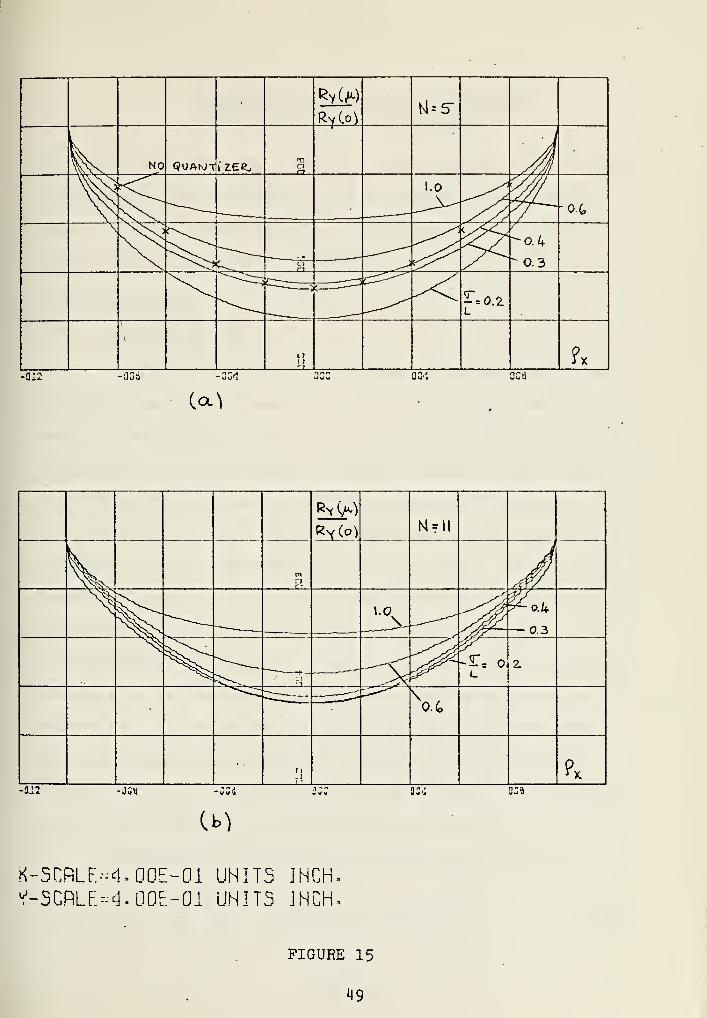
in the previous section apply for the plots of this caseRY (y)except that now the ordinate axis is e—r^r instead of py
since Y(t) is not zero mean. The results are shown on
Figure 15 for N equal to five and eleven.Ry(p)
It can be shown that for the case of no quantizer =—T-=-y
is given by
Rv (y) 1 + 2p„2
^m-—r^- (104)
Note how the curves of Figure 15 depart from the curve given
by (104) due to the effects of the quantizer.
In summary, in this chapter an algorithm has been devel-
oped suitable for computer programming in order to find the
autocorrelation function of the output of a quantizer (or
quantizer and a square law detector) given that the input
process is Gaussian and zero mean, and with known auto-
correlation function. What it basically does (for both cases)
is to reduce a double integral (75) and (100) into a single
integral by using the error function which is available in
most computer libraries.
47
V


The transfer curves for both cases, shown on Figures 8
through 14 and 15 are independent of the input process
providing it is Gaussian and has zero mean. These results
will be used in Chapter V.
48

-ill -J3W
LCL\
H = \\
V̂^ \.o
s
— 0.3
N^^ &*~r= o z
0.6
i
p.;24 3C9
CM
K-'SCRLF..-=4. 00E-01 UNITS INCH.
V-SCRLE=4- 00E-Q1 UNITS INCH,
FIGURE 15
19


V. DEGRADATION FACTOR CALCULATION WITHBOTH SAMPLING AND QUANTIZATION
In this 1 chapter the effects of sampling and quantization
on the performance figure of the two digital radiometers
under study are investigated. As in Chapter III, the two
cases will be considered separately.
A. IF SAMPLING
1. Exact Results
Refer to Figure 2. In Chapter III an expression was
developed for the degradation factor for the case where there
was no quantizer — see (30). Those results cannot be applied
directly to this case since in order to obtain (30) it was
assumed that q (kA) and q (kA) were samples of Gaussianc s
processes — see (22). With the addition of a quantizer it
is clear that this assumption no longer holds. Hence we
must start again with a more general approach. This can be
accomplished by concentrating first on the top channel of
the radiometer of Figure 2. The processing that the ADC and
computer do to the signal can be drawn sequentially as in
Figure 16. It is argued that the order in which the signal
q (t) is sampled and squared is immaterial as far as the
random variable I, is concerned. Hence Figure 16 is a valid
model of a channel of the radiometer of Figure 2.
' Referring to Figure 16 it follows that [Ref. 12]
a2
n-1a2
= JL + I i (l-£)[RY (kA) - E2[Y]] (105)
±1
n n k=l n i
50


R„(k ) is the k— sample of the autocorrelation function of
Y(t)
and
E[I,] = E[Y(t)] = al (106)
XcCO %l$\LAW
DETECTOR,
Y(t)
FIG!JRE 16
L\Xc^| ,^ (^Vc=»
Using (26) and the fact that for the case of Figure
2 the RF, Mixer, IF filter is symmetrical about f , then
« 2 o « 2°1
= 2°I.
(107)
and
E[I] = 2E[I,] = 2 o^ (108)
Applying the definition of degradation factor it
follows that
2a:
2 °Xc
4BEA n_1
kA 4
o4 *" <# k=it ^ q
[dE£ll
]2
dot
(109)
aX
atTop
c
51


Using the same argument as in Chapter III (A<<t) it
can be shown that the term
4BEA n-1
kA2 ^ CRY (kA)
k=l T 1 Mc
(110)
can be disregarded due to its small value compared with the
other terms in the numerator of (110).
Then (109) becomes
P^ =
2c% 4Bt.A n-1 h
ct V+sdr *[R
Y(kA) - VXr> Xr« k=l ^C
[ ffiEl ]2
daf:
(111)
at Top
Looking at (111) term by term, it is noted that in
the numerator, the first term can be obtained from (103) and
(95). The second term can be obtained from the correspondingRxc (kA)
value of 5
—
/ A \ . and the transfer characteristics of aRX C
(°)
quantizer followed by a square law detector (Figure 15).
Actually, a scale factor of av /o v will appear because of
the way the curves were normalized. The denominator can be
obtained from (95). Note however that Equations (93) » (95)
and the transfer characteristics developed In Chapter IV have
aY/L as a parameter and not crv . This is due to the choiceA X
c
of crx/L as a parameter since it was found in that chapter
that the ratio of a and L was of importance and not their
52

absolute magnitudes. Therefore it makes sense to have (111)
be a function of av /L at T instead of aY . av /L canAe
op Ac
Ac
be thought of as a normalized standard deviation of X (t) and
its value can be related to temperature in the same form as
Equations (10) and (11).
2 2 2A plot of E[I]/L versus cv /L is shown in
Ac
Figure 17 for different values of N. The effects of satura-
tion of the quantizer can be observed as temperature (equiva-
2 2lent to av / L ) is increased.
Ac
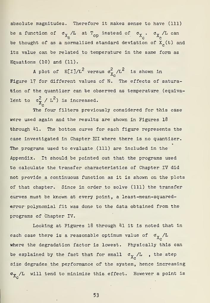
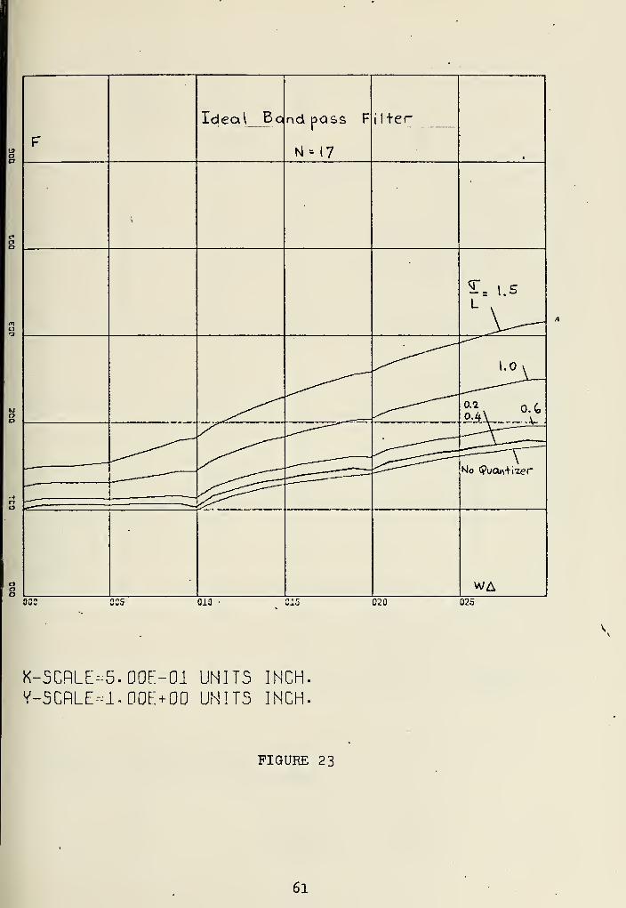
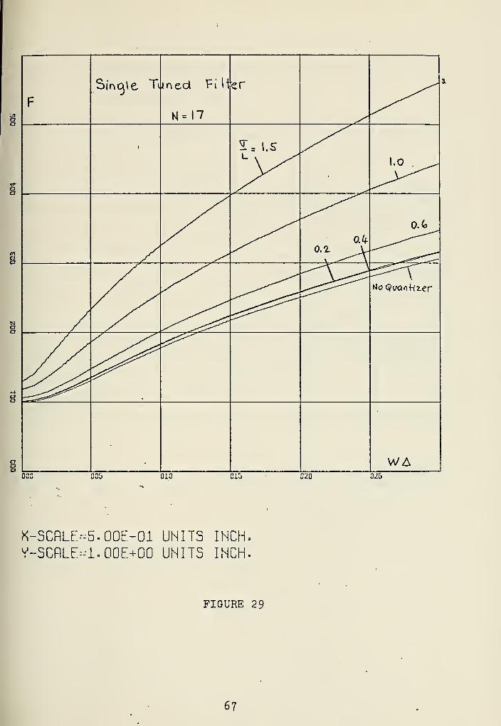
The four filters previously considered for this case
were used again and the results are shown in Figures 18
through kl. The bottom curve for each figure represents the
case investigated in Chapter III where there is no quantizer.
The programs used to evaluate (111) are included in the
Appendix. It should be pointed out that the programs used
to calculate the transfer characteristics of Chapter IV did
not provide a continuous function as it is shown on the plots
of that chapter. Since in order to solve (111) the transfer
curves must be known at every point, a least-mean-squared-
error polynomial fit was done to the data obtained from the
programs of Chapter IV.
Looking at Figures 18 through Hi it is noted that in
each case there is a reasonable optimum value of aY /LAc
where the degradation factor is lowest. Physically this can
be explained by the fact that for small a /L , the stepAc
size degrades the performance of the system, hence increasing
aY /L will tend to minimize this effect. However a point isAc
53


reached where saturation effects start dominating and the
further increase of a /L causes an increase of the
degradation factor. For N > 4 , av /L optimum is aroundAc
0.35 regardless of the sampling rate. This would imply that
for a given T , the gain setting of the RF, Mixer IF filter
should be set at a value such that av /L is equal to 0.35Ac
for optimum performance. Note that this optimality is for
small source temperatures. For large signals, dynamic range
is a problem. See Chapter VI.
2. An Approximation
The evaluation of (111) for the exact value of the
degradation factor requires extensive computer time. For a
quantizer of five bits or greater the computation time per
case is very long (on the order of hours). Therefore it is
of interest to investigate an approximate solution for the
degradation factor and to compare the results with the exact
values already obtained.
Figure 42 shows one of the channels of the radiometer
of Figure 2. Assume that the sampling rate is not too fast,
the step size of the quantizer is small with respect to the
standard deviation of the process X (t) and no saturationI
takes place in the quantizer. Then
q c(kA) = X
c(kA) + e
k(112)
where X (kA) is the k— sample of X (t) and e. Is a uniformly
distributed random variable that accounts for the error
introduced by the quantizer. The probability density
54


H
«0 "1
X XID ID
-1 —
I
en enI I
uj UJcj enen en
UJ U.J
_J _JCL CL
51 u Mb
55


1.1oF
Ideal Bar id pass Fi
M= 3
Iter
i
2". I.SL >
a s
,
'
,CL-—
-
MO
a4\,
^==^^
^ / ^No Quaofiz^r
o
oaoWA
03C 005 QJC Ci5 023
C
h-r'CflLE----5.'00F-01 UNITS INCH
V-SCRLE=1.00E+"00 UNITS INCH
FIGURE 18
02 E
56


13CI
F
Ideal Be r^d f>QSS Fi Iter
r
-
nLI
\
27, I.SL v __
1.0
MOn
0.3
0. 6N
No OuQn+iZer
CIs=— —
—
nC3o WA
0u2 (UO 3.15 020 025
X-5CRLE---5. 00E-01 UNITS INCH.
Y-3CRLE=1.00E+00 UNITS INCH.
FIGURE 19
57


ao
co
F
Ideal "Bqi\d pass, Fi 1+cr
CI
,
ST. ,.sL >
CMo 0.4
l.o
0.<o^ *__
S=no Qvan+izsJL-
-4r—
n
—
ooo WA0C5 OiO J-IU 020 02C
X-SCRLE=5.'00E-01 UNITS INCH.
V-SCRLE=1.00E+00 UNITS INCH.
FIGURE 20
58


13 P
Xdeal E><
U= 7
: ilter
a
t
inCI
•
-^qM
\.o
No QoQr\+izer
-1CIIT
^Z.
CIaCl
WAwo 020 025
K-SCRLE----5.00E-01 UNITS INCH.
V-SCRLE=I.00E+00 UNITS INCH.
FIGURE 21
59


aF
Ideal Ex *ndi pass ^•"{l+er
a
ft
\
\
L v
Mcr
1.0
0.2. O.GA
i
'
^"^
_~—-—~~—a4
No Qocun-hzer
-+
o «-=J - ^
aaoWA
ana 010 015 020 025
K-SCRLE-5.00E-0J UNITS INCH.
Y-SCRLE----1.00E + 00 UNITS INCH.
FIGURE 22
60

F
Idea\ Bo ad pass
H* 17
F il+er
{
T = i.sL
1.0 V
Mo <?ya»\+izer
•
-
WAoac oia 020 025
X-SCRLE-5. 00E-01 UNITS INCH-
Y-5CRLE=l.Q0E+00 UNITS INCH.
FIGURE 23
61


n
aa
naa
F
Sinc]\e Ty r
y1
10V ~s^
\
1
^x^O.2 0.4,
/
y y
//A/ </ y yf -y yy
/ y
-
WAQj.0 020 325
K-3CRLF.----5.00E-01 UNITS INCH.
V-SCRLE=l-00E+00 UNITS INCH-
FIGURE 24
62


F
Sing\e Tur\ed FdVer
\. ,.s ^1.0
^ 0.3^.
0. fc
/ 0.4
/ /
s ^No <?jQ^+i zer
//y^
/ SyS
W&oio 320 025
X-SCRLF--=5.00E-01 UNITS INCH.
V-SCRLE-1.00E+00 UNITS INCH.
FIGURE 25
63


Single T( Kr\ed Fi l+( !.r
i
s
l.C)^
0.6
°&^
^/^ ^^ No QuctA'H'z.er
^^>
03S ess oia us 1123 025
K-5CRLE=5.0QE-01 UNITS INCH.
V-SCRLE--U.00E + D0 UNITS INCH.
FIGURE 26
64


F
Single Ti tned Fi" 1 +
N=7
£T
-
L S< 1.(5^-
\ 0.4^
0.2.
z Jj^No(?L>a«hzcr
^^WA
do; 010 020 02b
X-SCRLE----5-00E-01 UNITS INCH.
V-SCRLE-LOOE+OO UNITS INCH.
FIGURE 27
65


a
F
Single T uned Pi 1
N = li-
ter ^r = i.s
1.0
0.4. J"0,<o^
/No <?uQfl-Hz:er
2*•
WAOJG 305 010 020 025
K-SCRLE----5. 00E-01 UNITS IHCH»
V-SCflLE=1.00E+D0 UNITS INCH.
FIGURE 28
66

X-SCRLE-5.00E-01 UNITS INCH.
V-SCRLE-LOOE+OO UNITS INCH.
FIGURE 29
67


F
Qotussia
N= 3
-
r B i.s-
L x l.o
\
0.2 ^^o.c
/^0.4^-
^ i^o Quantizer
-..
WAaoc a;a 022 025
K-SCRLE----5.0GE-G1 'UNITS INCH.
V-SCRLE=1.0QF.+00 UNITS INCH.
FIGURE 30
68


Qaussiar\ Filter
LICIrr
F
M* 4-
r..i.s-
\ **
1.0 ^^13
0.3 ^^^\^0Jo±^-
ttA^
____> .^
No (Ji/cMKzer
~-r<^~l
n
s-
on WA3 S3 OJ0 020 02S
K-5CflLE-5.00F-01 UNITS INCH.
V-SCRLE--U.00E+00 UNITS INCH*
FIGURE 31
69


ao
mao
Noo
F
GoUSSiQ a F M i-er
N = 5"
i
-
I.l.s1.(3^.
°'t^^^
0,2
Mo QiKm+Vter
WAace 0:0 1 "^ 020 025
K-SCnLE-5.00F.-01 UNITS INCH-
Y-SCRLE---1.00E+00 UNITS INCH.
FIGURE 32
70

LIO
F
_Qaussia a, Filter
a
-
PIa
\
ST. V.SL v i.o
MD
D-/f^
Mo Qua^+iicr
-1
. —
-
—
CICID
W&S3; CC5 013 315 023 flJS
"K-SCRLE--5- 00E-01 UNITS INCH.
V-SCRLE=l-0DE+00 UNITS INCH.
FIGURE 33
71


a F
Cjauss ia n, Pil-Ver
o
-
mo
L v.
-^^1.0
tsio
o.h Jl0.6
Ho QoQia+izer
C7Oow/\
On* 010 215 020 025
X-SCRLE=5.00E-01 UNITS INCH.
Y-SCflLE=l-00E+00 UNITS INCH.
FIGURE 34
72


13f
C=\a ^ssi<
M= 17
r
o
t
na
L y 1.0
a
0.2,0. if
o. G
No Qucmhzer
-i
C7ooWA
as: CCS 010 C.15 02Q 02S
K-5CRLE=5« 00E-01 UNITS INCH.
Y-SCRLE=l.QQE+00 UNITS INCH.
FIGURE 35
73


BUTTE ft V'ORTH Fll_TE£.
FN = 3 ^
£. i.sI.O
0.2^-"^
O.C
0.4
/
=^ Mo Quantizer
*
WAi 313 315 32a 325
K-SCRLE-S-OOE-Ol UNITS INCH,
V-SCRLE-l.OOE+00 UNITS INCH.
FIGURE 36
74


-
BUTTER.WO R.TH F\LTE fc.
\3F N= 4-
\
tfa
l
L"
N
l.SI.Oi^
^ 0.3^^-^-^\^~oA^
i
0.4^a r ^^^__^
y ^^No Quao-tv'ier
—i-
aa^^^
a WA02: DCS 010 015 020 CiS
k-scple-^cde-ol units inch.
y-scrle-i. ooe+oo units inch.
FIGURE 37
75


a
FBUTTEdW
M= 5"
OR.TH F\l_-"Eft.
<*-
cr
!
\
r = i.s
1.0
O.t0^\_
~t
Mo Quantizer
n
aaa
WA010 020 025
rt-SCRLE=5.00E-01 UNJTS INCH.
V-SCRLE-LOOE+OO UNITS INCH.
FIGURE 38
76


Li
FBUTTER.W(JR.TH Ft LI Eft,
LO^
. o. t
"^--i^
0^^
,
^~*""*^
^^^^
No QyQirvi-iier
n — "
—
~~*~cIlZ^
aaa
WAas: 010 015 02a 025
ft-SCRLE-5. DDE-01 UNITS INCH.
V-SCnLE-i.ODE+00 UNITS INCH,
FIGURE 39
77


oF
BUTTEdv
NUll
;o<lTH F ILTEFL
a-CI
i
'-
nL. y
i.o
o
1 ^ o.k
0.2
o.c>
_/.^^ Mo QvdAti zer
-H
CJo WAluti
nnr.Uuw OiO Ci5 020 02D
X-SCRLE=5."00E-Q1 UNITS INCH.
V-SCflLE=1.00E+00 UNITS INCH.
FIGURE 40
78


K-SCRLE-5- DDE-01 UNITS INCH,
Y-5CRLE=1. OOE+00 UNITS INCH.
FIGURE 41
79


function of ek
is the following [Ref. 13]
f(ek ) =
1
a- S. < e < £
2ek 2
(113)
Then
n nXl =
n"kfx
qc^kA) ' n-
k^[X
c(kA) + 2ekV kA) + e
k ] (114)
and
E[I1
]i Z ECX^(kA)] + .£ Z E[2e.X
p(kA)] + i Z E[e£]
nk=]_
c nk=1
k c nk=1
k (115)
^Mfk-i
FIGURE 42
I,
80


Assuming e, and X_(kA) are uncorrelated, which is a
good assumption if the step size is small compared with o .
Xc
2 a2
E[I1 ] = ^x
+12 (116)
c
Now
E[I2] = -4-E [ £ x2(jA) + 2 E e.X (jA) + E e
2] •
n j=lC
j=l J Cj=l J
(117)
[ E XT(kA) + 2 E e. X (kA) E e2
]
k=lc
k=lK c
k=l*
Expanding (117) and using (23) and the assumption
that e, and e. are independent for k / j, which is good ifK J
the sampling rate is slow, it follows that
"f,= ^r + 4 j,
c**>4 (k»)*jr £ 4. + J A <
118 >
It was shown previously that for the case of Figure
2, if H (f) was symmetrical about f , then
a2
= 2a2
(119)x x
l
and
ECI] = 2 E[I1 ] (120)
81


Using (119) and (120) it follows that
2V "Z1„ k_2 „., , 1 a
2 „. a4
^ = BEA + -?- * (1 " ^ ^ CkA) + F "ITV +
-T- 350 V (121)ax ^= "'" c x ay
c c c
But the first two terms are just the degradation
factor for the case of no quantizer, therefore (121) can be
written as
*2 - PN« * \ 4- V +350 TT V < 122 >
where PNQ is the degradation factor with no quantizer. The
last two terms of (122) represent a correction, due to
quantization, for the degradation factor with no quantizer.
The approximate solution is very good if the assump-
tions under which it was derived hold. For N=17, o^ /L = 0.3c
(a/cr„ = 0.42) and WA= 1.0 the error is less than one percent.c
For values of a /L greater than 0.3 the approximation is not
good due to saturation. For values much smaller, it again
fails due to the large value of a/av . Figure 43 shows how
the two results compare for N=7 and different values of
a„ /L. In it, the behavior of the two 'solutions as o /L isc ! c
increased can be observed. For N much greater than 7, the
approximation is very good when ov /L is near 0.3.*c
82


•J)F
Qouss ia r\, Pj Her
M
5!. i.o x
/"-^J^£**" Mo <JvK»ttti zer
___^/ ^ Approximation
Q -3/L r 0. If
^ %-- o. &
A Vl= i.o"1 \-pr~Er¥\~?k~~vI
LICID
aCI
-
WAJgu 225 Oifl C15 020 D25
K-SCRLE-5- 00E-01 UNITS INCH.
Y-SCRLE----5- 00E-01 UNITS INCH-
FIGURE 43
83


B. RC FILTERING THEN SAMPLING
Refer to Figure 3. Unfortunately there is no exact
solution for this case since there is no way to get the
second order probability density function of the process
z(t). This would be needed to approach the problem in the
same way as done for the radiometer of Figure 2. Two
approximations will be discussed.
1. First Approximation
It was shown in Chapter III that
and
E[Z] = g(NQ/2) (123)
4 - S2
<V2)2 2B^ < 124 >
Owing to the Central Limit Theorem It can be assumed
that z(t) is a Gaussian process if Bp t Rr,>> 1 . Due to the
square law detector, it is obvious that z(t) can never be
negative, hence the assumption is good only if the mean of
z(t) is sufficiently large compared to its standard
deviation so that the assumed Gaussian probability density
function Is negligible for negative arguments.
It is also assumed that the quantizer has a bias 'b'
as shown on Figure 44. When b=0 this quantizer reduces to
the one shown in Figure 7. It is argued that the order in
which z(t) is sampled and quantized is immaterial as far as
the output I is concerned. Hence Figure 45 is a valid model
of the processing done by the ADC and computer.
84


-0
1
z
-- ><
*"
.=3-
aOH
2
o+- cr-
85


Z(tO g_W x^gN £>Vm i I
FIGURE 45
Let
E[Z] = m (125)
then the probability density function of z(t) is
fz(z) =
(2Tra?)?2
(z-m)'
o 2
(126)
It can be shown, using a procedure similar to that
introduced in Chapter IV that
N q, X.H7}
E[q(t)] = E -± [ erf(-J
i=l (2)%
X. --m.) _ erf(-±4—) ] (127)
Z
Xj-m
(2)%
V pz>"
NE q.
-32/2
(2tt)^ i-1X
Xj^-mL
dB (128)
Nqj
j=i2 r
iKp~,B) = E 4- |erf[
X^-m- P^B
Vl"*1
^(l-p2,)]1*
] - erf
[
0„- ~ pz6
^(l-p2)]
1*1
] (129)
86


and
But from Figure 44
X±
= 21.(1 - |)/(H-1) + b (130)
q±= 2L[i - (N+l)/2]/(N-l) (131)
Equation (130) can be written as
X, = X + b (132)1 o
±
where X is the value of X. when the quantizer is zero°i
i
centered.
Substituting (131) and (132) into Equations (127)
through (129), the parameter b-m appears. Physically, this
is the offset of the mean of the process z(t) with respect
to the center of the quantizer. When no source is present
the value of this offset will be determined by the quiescent
conditions of the radiometer. When looking at a source,
however, the value of the offset will change since the mean
of z(t) changes linearly with temperature.
Let
f = mQ
- b {133)
where m is the expected value of z(t) at T . Then (127)
through (129) can be written as
87


N qj , X^ ~ f « H2Btm )h
(az - az )
= a7 Z — { erf[ r ]Z
i=l a' I (2)^'
E[q(t)] _L "'
''Z * ^' UZ
(134)
. erf[ -i T gj " zo - ^3}
^i-l " f ' +(2BtRC^ (°Z " az ) ^
(2)%a''Z
az'
Rq(pZ )
j
N q» -B2/2
-S5 h- 2 jr , ' *,
(pz,B)e d6 (135)
T2
(2ir)*i-laZ Xo i-f Z
*'(p7 ,B)= 1 -1- JerfC -£ 5-t- ] - erf [
£ s-r— ] (136)Z
j=l 2az
I C2(l-<72)]
2 [2(l-a2)T* J
where a „ is the value of the standard deviation of z(t) at
T , and all primed variables imply that they have been
normalized by L.
For the case of p„ = 1 (135) becomes
E[- 2
nN q'
2Xq. - f
'
XL - f'EO = Si
[erf (-2*-
) - erf (
1-1^ )] (137)
c^ i=l 2cz
az(2)^ a
z(2)^
Equations (13*0 through (137) can be solved in the
same form as done in Chapter III. However, the addition of
88


two new parameters, (f and (2Bt RC)'5
) , makes the problem
difficult to solve in a general way due to the number of
variables involved.
One way to get around this problem is to assume that
(2B„t nr,P is large. Then'E"RC-
NXi
E[q] = Z q. / f7 (z,m,a) dz (138)1=1 X
i-1
where
(z-m) 2
~ 2
f7 (z,m,a) = K-r- e2a
(139)
From (123) and (124)
m = ozC2BE
tRC
)'s (140)
Therefore
-,„ N X. df 7 (z,m,a) dz
i- * 11 / -Lsa (m)
but
dfZ _ 9f
+3f da
(142)dm 9m 9a dm
Substituting into (l4l) and using the fact that
55T " - If (l43)9m 9z
89

it follows that
, N N X df
f = ^W * qi[f
z(Xi_1
,m,a)-fz(Xi,m,a)] + Z q±
Z1 ^ da (144)
X-X X-X A. -
1 /
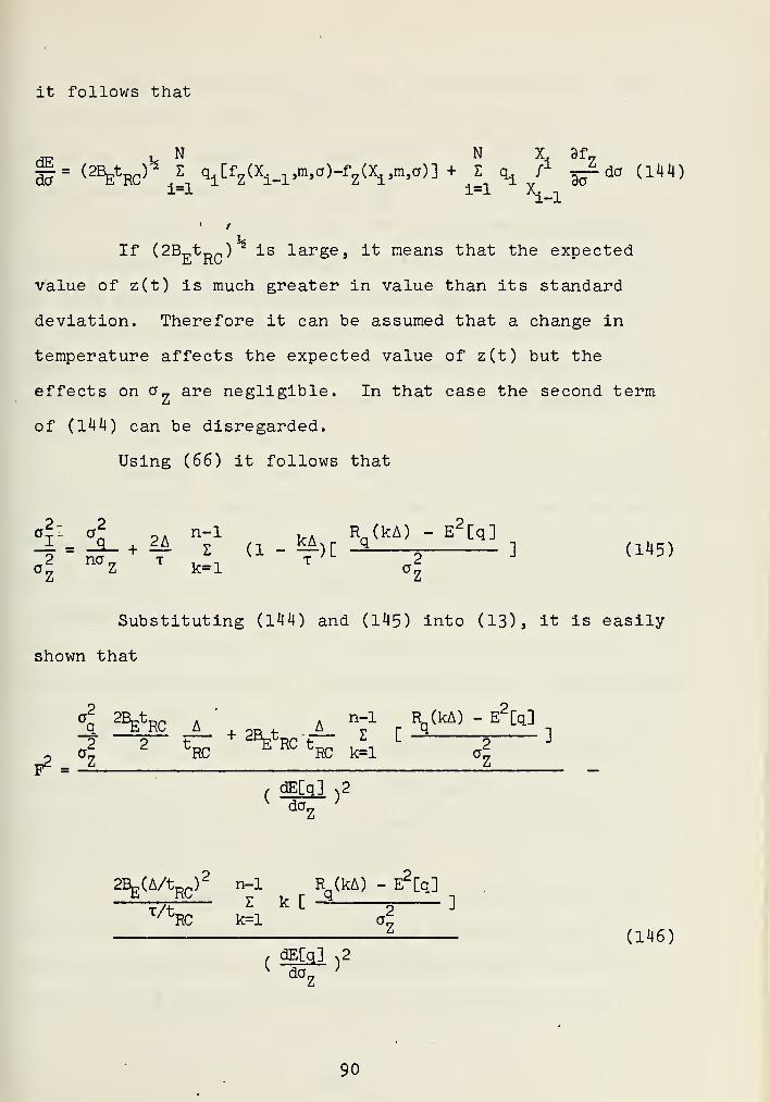
%If (2BFt RC ) Is large, it means that the expected
value of z(t) is much greater in value than its standard
deviation. Therefore it can be assumed that a change in
temperature affects the expected value of z(t) but the
effects onff„ are negligible. In that case the second term
of (144) can be disregarded.
Using (66) it follows that
°I: a
o 2An" 1 kA R
a(kA) " E [q]4=^- + ¥ E u - ^H -
5 1 0145)
°Z Z k=1 °Z
Substituting (144) and (145) into (13), it is easily
shown that
a'
« ^RC A '
+_
± A ^ Rqto) - E
2M.2 2 t™ ^ETRC ~t™ , \ L
_2J
o Gz
RC RC k=l az
(dECq] )2
1 daZ
J
2BE(A/t
RC )2 n-1 R
q(kA) - E
2[q]
T/rRC k=l a
z
, dE[q] v2
(146)
90


The parameter 2BEt RC on the numerator of (146) will
cancel out. The third term of (146) can be neglected only
if T>>tR „ (see comments in Chapter III. The addition of a
quantizer does not invalidate them).
It must be pointed out that the parameter (2BptRC ) ,
even though it does not appear in (146), is an important one.
It is a measure of how much smoothing the RC filter does.
A large value makes quantization difficult. On the other
hand, a small value invalidates the assumption that z(t) is
a Gaussian process. Other consequences of this parameter
will be discussed in Chapter VI.
Equation (146) can be evaluated using (13*0 through
(137) and (144). Basically it is done in the same form as
for the case discussed in Section A of this chapter. Using
(135) and (136) a set of transfer characteristics has to be
computed similar to Figures 8 through 14 (that set of curves
is the solution when f'=0). The major difficulty lies in
the additional parameter f which increases the dimensionality
of the problem.
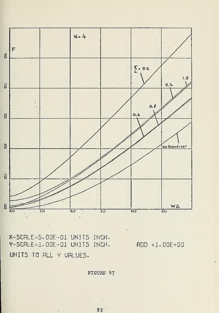
The case when f'=0 (no offset) was analyzed using
Figures 8 through 14 and (144). The results are shown in
Figures 46 through 51. For any other value of f (134)
through (137) have to be evaluated.
As an example the case of N=13, az/L=0.2 and f'=0.5
was solved. The results are shown in Figures 52 and 53-
Note that they are very close to the zero offset case for a
seven level quantizer with az/L=0.4. The reason is that
91


Sl=3 / /13CI
F / //
9Ir 0.3U y
o.W / I.Sy
o o.i> yyy/ V// °\A
y/3 / ,/%/
M/ VV
»io QuQrtfiier
/ Asy/
CD
^ ^5^
a WAazz Qia 02 J 02i
K-SCRLE-5.00E-01 UNITS INCH.
V-SCflLE-l-OOE-Ol UNITS INCH. RDD +1.00E+00
UNITS TO RLL V URLUES-
FIGURE 46
92

F
N-4
E = O.2. /I.S
oi, y
\
o.s >/
No QuQnti ter
W&as: OiO 020 025
X-5CRLE-5- OOE-01 UNITS INCHV-SCRLE-1. 00E-G1 UNITS INCH
UNITS TO RLL V URLUES.
RDD +1.00E+00
FIGURE 47
93


LIOO
N=S /F /
/
L. v /
0.4/ /
0.& / y^y•
/ o.fc y\ y^y/yy / rlo (Juan+irer
W&ooc buy 010 ZI'j 02a 025
K-SCRLE----5. 00E-01 UNITS INCH.
Y-SCRLE----1.00E-01 UNITS inch.
UNITS TO RLL V URLUES-
RDD +1.00E+00
FIGURE 48
94


OO
F
KU7
t
/.
\J1.5 //
0X
< ^ No QvQn+i'zcr
W&013 020 025
K-SC.RLE----5.0DE-01 UNITS INCH.
Y-5CRLE=i..00E-01 UNITS INCH.
UNITS TO RLL V URLUE5.
RDD +1-DDE+00
FIGURE 49
95


n
O
no
FNU l\
\
\ // 0XS?
Ho QutM-Hzec
y^' ^
// \>
jS* ^P ^>
WAOiO 020 02u
X-SCRLE-5.00E-01 UNITS INCH.
*-SCnLF.----l.QOE-Ql UNITS INCH.
UNITS TO RLL V URLUES.
RDD +1.00E+00
FIGURE 50
96


11
IT
F
N-I7\
i
/ 0.8 ,
^^ 0.2
No <?v/cu-Kz.er
\/ *rs^y'
y S^yS
W&010 020 . D25
K-SCRLE----5- 00E-01 UNITS INCH,
Y-5CRLE=1. OOE-01 UNITS INCH.
UNITS TO RLL V URLUES-
RDD +L-QOE+00
FIGURE 51
97


N=13
i = o.s
-= o.;l
—
o
n
C)CI
... — -.^
-oi; -003 OGi 003
k-SCflLE=4-:00E-01 UNITS INCH.
y-senLE-4.ooF.-oi units inch.
FIGURE 52
98


F $-- 0.5
^
£ s 0.2.L
do Gvanh'z-cr
AJ?Q Second
> ,vA4^^^^ WA
tzi- UUU OiO 315 323 025
X-SCRLE--=5.00E-01 UNITS INCH.
V-SCRLE-LOOE-Ol UNITS INCH.
UNITS TO RLL V URLUES-
RDD +1.00E+00
FIGURE 53
99


te3^
K-SCRLE----5. OOE-01 UNITS INCH.
Y-SCRLE-JL OOE-.Ol UNITS INCH.
UNITS TO RLL V URLUES.
ROD +1-OOE+GO
FIGURE 54
100


a/az
is the same for both cases. They are not exactly
equal however, since In one case clipping occurs essentially
for positive values of the signal, while in the other case
clipping occurs symmetrically for both positive and negative
values of signal. Figure 52 is a plot of the transfer char-
acteristics for this example. The programs used are in the
appendix (See "Transfer Characteristics of Quantizer With
Offset," and "RC Filtering Then Sampling, Offset Case").
The case when N=2, f'=0 is of interest since results
are obtained easily without extensive computer programming.
Using (146) and (96) it can be shown that
o w a an~1 VkA > \r n"1 VkA)
^*4 + 4 A "-jpbt -it &*"<** isr(147)
tRC
The last term can be neglected when x>>t RC . As the
sampling rate increases, A goes to zero and Equation (147)
becomes
F2 = / arcsin e" y dy (148)
For large x , the upper limit can be replaced by
infinity and (148) integrates to
F2 = \ In 2 (149)
therefore
F = 1.04 (150)
101


The results are surprising since it means that a
hard limiter degrades the system only by four percent.
However, the dynamic range of a radiometer using a hard
limiter would be very small hence this result is of little
practical use. More on the problem of dynamic range will
be discussed in Chapter VI.
2. Second Approximation
Using the same arguments as in part A of this
chapter, it can be shown that [Ref. 9]
f2
- pno + r—t~ (151)m t
RC ct^24
The results obtained from (151) are in close agree-
ment with those obtained using the first approximation even
for low values of N. It must be kept in mind that the
second approximation does not take into account saturation
effects of- the quantizer. For the case when f '=0 it was
found that if a /L < .6 WA > 1 , a/a < 2 and N > 5,
the second approximation was within 1.5 percent of the first
(For N=17 and the above conditions, the difference was less
than 0.6 percent). These results indicate that a sizable
amount of saturation can occur before (151) no longer holds.
Figure 53 shows how the two approximation compare for the
example done on page 91. Figure 5^ shows a comparison for
N=7, f'=0 and different values of a /L. The differentZ
behavior of the two approximations as a„/L is increased can
be observed.
102


To summarize, in this chapter an exact solution has
been found for degradation factor of the radiometer of
Figure 2. For the radiometer of Figure 3 no such solution
exists, but an approximation can be made under the reasonably
good assumption that z(t) is a Gaussian random process. For
both cases the major difficulty in global analysis lies in
the number of parameters involved.
An approximate solution was developed which is in
close agreement with the first solution. Its major advantage
is that it is easy to compute and as the number of steps
increases, it gets better. For practical ADC it should be
adequate.
103


VI. DYNAMIC RANGE AND LINEARITY OF A DIGITAL RADIOMETER
In this chapter the effects of the addition of an ADC
on the linearity of theoutput of a radiometer is investigated.
The main problem here is the saturation effect of the
quantizer.
A. IF SAMPLING
Refer to Figure 2. The output voltage versus temperature
characteristics for this case was investigated previously,
and Is shown in Figure 17. If the ADC was ideal (no satura-
tion and a/a =0) there would be one straight-line curve
with slope equal to two. It can be seen that for small
av2/l2 (proportional to temperature) the curves tend to haveAc
a slope of two.
Figure 17 provides all the information needed for the
problem under investigation in this chapter. However, the
way the curves were normalized makes them awkward to use.
They can be changed starting with (108) and (95).
2
-, rT naX N q' 2 X! X' ,
V^
^¥- - ~f"
S (=£-) [erf (-r-^-p ) - erf (-r^- 1 (152)If IT 1=1 a
X aX (2) °X (2)
but
% 2
TT =(N-l)a/ay
(153)Ac
104


Therefore (152) becomes
E[I] <4 N q^(N-l) 2f
x; (N-l) X^CN-1) >
-V" = —p- s [?CT 75 1 lerf[ r ] - erf[ p ] f
(154)a2
a2
1=12aX/ a
I 2(2)^av/a 2(2)^cv /a J— Va 2u;ax
c c
Equation (154) is plotted in Figure 55. The curves asymptote
to
sol = m£- (155)a
This can be shown by using the fact thas as cr„/a
gets large the quantizer appears as a hard limiter.
Figure 55 shows that a substantial range of linear
output can be obtained with this scheme before saturation
dominates.
In order to use Figure 55 a criterion must be
defined for how much departure from linearity is allowed
for the temperature range expected (one percent, for example).
Once that is defined, Figure 55 can be entered to determine
the number of steps of the quantizer required. The value of
the abscissa at T will be determined mainly by how muchop
degradation of performance is allowed (Chapter V). We thus
have a trade-off of linear dynamic range versus minimum
detectable temperature AT.
105


\ xi
H--17/1.1Mn
ECi3
a2 ii^^-
CJ
n
—i
i
/ ^
7
oo
5
LICJO
4
>
3
CIan
5**
a*:c6 0C3 oi: 015
X-SCRlE-3.00E+00 UNITS INCH.
V-SCflLE-5. 00E+00 UNITS INCH.
FIGURE 55
106

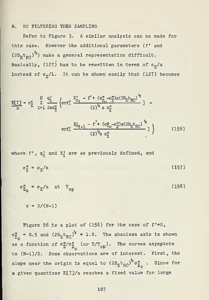
B. RC FILTERING THEN SAMPLING
Refer to Figure 3- A similar analysis can be made for
this case. However the additional parameters (f and
(2BEtRC)'1
) make a general representation difficult.
Basically, (127) has to be rewritten in terms of a„/a
instead of a7/L. It can be shown easily that (127) becomes
N q! , ^ -f' + (qgn^)s(2BEtRC)^ _
(2)%
s a£
in q: ,
E[I] = o" Z -±- 4erf[—T 1=1 2sa" <•
X£, - f + (ag -<j")s(2BFt )2
^
erf[ -^=1 j=2_Z ^ RC
] i (156)(2)^s a£
_
J
where f' , q! and X! are as previously defined, and
a£ = az/a (157)
a" = a 7/a at T (158)Z Z op
s = 2/(N-l)
Figure 56 is a plot of (156) for the case of f'=0,
wa£ =0.5 and (2Bc,t TDr,) = 1.0. The abscissa axis is shown
as a function of crg/a^ (or T/T ) . The curves asymptoteo
to (N-D/2. Some observations are of interest. First, the
hslope near the origin is equal to (2B
EtRC ) a£ . Since for
a given quantizer E[I]/a reaches a fixed value for large
107


-1
\
nC)
ECUa2-
t
Mr 17
10
(1
7
Ma
^5
""4
3
C7
0:2 OS-J 026 3C9 010
K-SGRLE-2. 00E+00 UNITS INCH.
V-SCRLE----2.00E+00 UNITS INCH.
FIGURE 56
108


values of crj/ag , increasing ( 2BEtRC ) (which physically
omeans that more smoothing will be done by the RC filter)
decreases the range of linear output. Therefore tR~ should
be chosen as the minimum value which will enable the sampler
to operate properly. Second, the parameter a 1
! will beLo
determined by the amount of degradation tolerated at Top
And third,. the desired range of linear output will determine
the number of steps of the quantizer. Therefore a procedure
to use a Figure such as 56 would be as follows: First,
determine (2BEt RC)^ and a" using the criteria given above.
Second, draw a set of curves of the expected value of the
output versus temperature using (156). Third, decide upon
a criterion of how much departure from linearity is allowed
in the temperature range of operation, and finally obtain
the required number of steps from the curves drawn.
To summarize, the effects of the addition of an ADC on
the linearity of the output of the radiometers under
consideration, have been investigated in this chapter. The
knowledge of the behavior of the output is important for
calibration purposes.
-m.-'-
109


values of cr£/cr£ , Increasing ( 2BEtRC ) (which physically
means that more smoothing will be done by the RC filter)
decreases the range of linear output. Therefore tD„ should
be chosen as the minimum value which will enable the sampler
to operate properly. Second, the parameter o% will be
determined by the amount of degradation tolerated at Top
And third,. the desired range of linear output will determine
the number of steps of the quantizer. Therefore a procedure
to use a Figure such as 56 would be as follows: First,
determine (2BEt RC ) and a" using the criteria given above.
oSecond, draw a set of curves of the expected value of the
output versus temperature using (156). Third, decide upon
a criterion of how much departure from linearity is allowed
in the temperature range of operation, and finally obtain
the required number of steps from the curves drawn.
To summarize, the effects of the addition of an ADC on
the linearity of the output of the radiometers under
consideration, have been investigated in this chapter. The
knowledge of the behavior of the output is important for
calibration purposes.
109


where F is the degradation factor for the equivalent total
power radiometer. The factor multiplying F is the performance
figure of a balanced Dicke radiometer.
()-®-nVM»!-k--»
FIGURE 57
Equation (160) follows from the fact that for the half
of the switching cycle that the radiometer is connected to
the source^ it behaves as a total power radiometer.
Care must be taken however on the selection of t. If
commencement of sampling is delayed after switching, it must
be corrected for the loss in integration time. Also, for
the case of RC filtering followed by sampling, the introduc-
tion of the RC filter must be reflected in an increase of t
since F takes only into account the effects of the inclusion
of the ADC.
The problem of dynamic range and linearity of the output
can be handled with the curves developed in Chapter VI.
Ill


H
o
!A]- c
- I
II
-*I
I
I—I—o
~1
OP
01
_i
US £Qi O<E -, UJ
^ -» /a
ooITV
W
OH
o
>--- — __i
—VW-
112


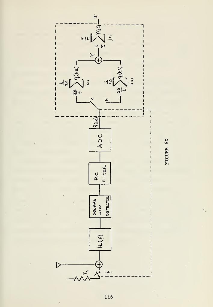
B. NOISE ADDING RADIOMETER
Figures 59 and 60 show two digital noise adding radio-
meters. The one in Figure 59 corresponds to the IF sampling
case and only one channel is shown. The one in Figure 60
corresponds to the RC filtering case. The extension of
results already found to NAR is considerably more difficult
than for a balanced Dicke radiometer. This is due to the
processing involved [Ref. 13]
•
Let
and
I = E + e (161)n n n
Io
= EQ
+ eo
(162)
where I and I are the outputs of the radiometer withnoT +T and T _ respectively. E_ and E^ are the expectedop n op n o
value of the output for the case of T +T and T respec-* op n op *
tively. e and e are independent, zero mean random variables
with standard deviation equal to a, and aT , and represent
n o
the deviation from the mean for a particular measurement
(one cycle).
Then the Y-factor is [Ref. 14]
enI E^ 1 + p2-
Y = -a = gH [En ] (163)
o o e
1 + ^
113


If enand e
oare small compared with E and E , then
E E
Y = — [ l + JlE^ L x
En
E.(164)
EE[Y] = =£
Eo
(165)
and
a 2 = c*a
]2
C(in) 2 ^,-(i°) 2
]
n
Using Equation (166) and the fact that for a NAR
(166)
.AT. . (1 + ^ < _i_ ,*
op n E(167)
where t is the switching period; for the case of Figure 2
it can be shown by straight substitution that,
1r ,
dE"n] gdo
x
NAR
aX dE[I ]
2( 1+^ F
n+
<—2^- >
2
X XT +T ° .... E[I J.op n o
O^p_
(1 +
2d^n ]
o,2 r .2— ) [ dcx
n E[In ]
dE[Io ]
da'
T +Tn op
ettin' "op
(168)
where c\r is a,r at T ., ov is a v at TX op' Xn X n.
114


4
>-
Q>
<3
Of
1
-it
AAAA3
CTk
M
115

hL
1 v\v
-^i m
1 1
^l ;
1 ^1 M. I 1
j1
o zi :
* r
'3"
i 8^2 HiOr <T UJ(0 -» a
-
o
D> -d5
o
M
AAA—-J-AAA
116


F is the degradation factor of the corresponding total
power radiometer at T=T +T , and F is the degradationn op o °
factor of the corresponding total power radiometer at T=Top
For the case of Figure 3, o„ must be replaced by a„ in (168).
All the terms of (168) can be calculated from equations
previously developed.
It must be noted that for the case when the signal is
filtered before sampling (Figure 60), f (offset) cannot be
zero at T ^ or T +T since the ADC would give zero output,op op n to ^
The problem of dynamic range and linearity is easy to
handle. From Figures 55 or 56, depending on the system under
consideration, and (165) a plot can be made relating E[I]
to temperature. Figure 6l shows how this is done for the
system of Figure 59.
In summary, in this chapter the results obtained in the
six previous chapters for the digital total power radiometers
shown in Figures 2 and 3, have been used to determine
performance of other digital radiometers. The balanced
Dicke and noise adding radiometers were investigated. For
the balanced Dicke radiometer, there is a simple and straight-
forward relationship. For the NAR, however, a relationship
was found but it is more involved. The problem of dynamic
range and linearity can be handled easily.
117


ECUa 1-
<
-
!
E„ Ec
>ecn- E- Cx3= £yE o
°%*02.: GC6 3nr 012 015
X-SCRLE-3.00E+00 UNITS INCH.
Y-SCRLE---3.00E+00 UNITS INCH.
FIGURE 61
118


VIII. DIGITAL FILTERING
In the analysis of the classical total power radiometer
an Integrator is used to smooth the output signal. This
scheme works well but it has the disadvantage that it gives
output information only at discrete intervals of time, corre-
sponding to blocks of data. Such performance might not be
acceptable in some cases because a smooth output might be
desirable. Therefore, a pure integrator is not generally
used but rather a low pass filter (such as a RC) that pro-
vides a continuous output. The theory and equations of a
classical total power radiometer do not change when using
these low pass filters instead of an integrator if an
equivalent integration time is defined [Ref. $].
The digital total power radiometers of Figures 2 and 3
suffer the same disadvantage as the classical TPR. That is,
output information is obtained only after the summers have
completed the summation of the n samples. Therefore a scheme
where output information is obtained more often must be
investigated. This chapter deals with the substitution of
the summers of Figures 2 and 3 by digital filters. There is
an additional reason for wanting to do this analysis. Since
a computer is already being used in the radiometers of
Figures 2 and 3, the use of a digital filter often does not
require any more hardware.
Figure 62 shows a digital filter operating on a digital
signal X. . The filter is characterized by its impulse
119

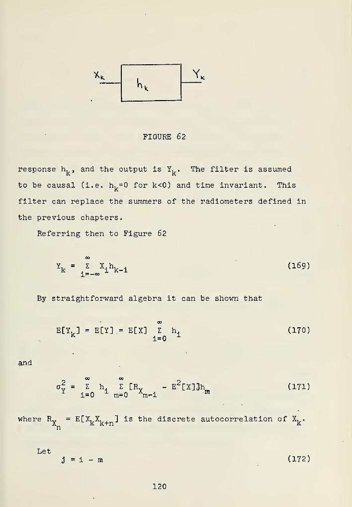
FIGURE 62
response h, , and the output is Y, . The filter is assumed
to be causal (i.e. h, =0 for k<0) and time invariant. This
filter can replace the summers of the radiometers defined in
the previous chapters.
Referring then to Figure 62
Yk - E xi\-i
i=-oo(169)
By straightforward algebra it can be shown that
E[Y, ] = E[Y] = E[X] E h,K
i=01
(170)
and
o-J = Eh, E [RY - E^CXirjh^Y
i=01 m=0
Xm-i m(171)
where Rv = E[X, X. , ] is the discrete autocorrelation of X, .
X k k+n kn
LetJ = i - m (172)
120


then
Oy = E h E [R - E*[X]]h, , (173)
Assume that h decays much slower than Rv . This can be•J
Xj
seen by observing the location where this filter would go
in Figures 2 and 3- For the case of Figure 2, the power
spectral density at the input of the digital filters is
shaped by the RF, Mixer, IF filter which is broad-band.
For the case of Figure 3, it can be assumed only when t Rf,
is small (this is the case for which Figures 46 through 51
apply).
Then (173) becomes
oo 4
2aY
=
±l Qhi jf_„
CRXj - E
2[X]]h
±(174)
Let j be the value where R(j ) is negligible. Then
(17^) can be rewritten as
o i °° iE h
2E [R„ - E 2 [X3] + E h
2E [RY - E
2[X]]
i=0x j— A
j i=i 1 1=-oo A1
a; = 2 h
(175)
It can be shown that the first summation is much smaller
than the second, and hence it can be ignored. Furthermore
the limits of the second summation can be changed as follows
2without altering the value of a y significantly
121


a2
= E h2
E [R - E2[X]]
i=0 j=-°° j
(176)
For the summer used in previous chapters, it can be shown
(using the same notation of Figure 62) that
a2
= a2
+ 2n E [R - E2[X]]- 2n E £ [Ry - E
2[X]] (177)
1 A k=l Ak k=l
n*k
and
E[Y] = E[X] (178)
The upper limit of the summation of (177) can be replaced
by infinity (due to the narrowness of RY ,(u)) and the third
term can be ignored (see Chapters III and V).
Substituting (170) and (176) into (4) for the general
digital filter, it follows that
oF>2
op
o °° °°
P E h. + p- E h.
Tj_ i=0J
T__ i=0x
j=l *jE [Ry - E
2[X]]
op op
(zh )2(
dED0)21-0
*
dTop
(179)
Doing the same with (177) and (178) it follows that
op
n T™2E [Ry -
nV k=l *kE2[X]]
rdECXl-,2L dT J
(180)Top
122

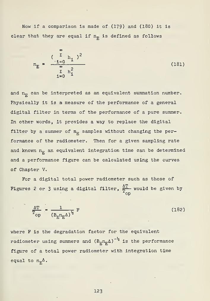
Now if a comparison is made of (179) and (180) it is
clear that they are equal if np is defined as follows
c2
h, )2
-E -
1:° - (18DZ tu
i=0 x
and n„ can be interpreted as an equivalent summation number.
Physically it is a measure of the performance of a general
digital filter in terms of the performance of a pure summer.
In other words, it provides a way to replace the digital
filter by a summer of np samples without changing the per-
formance of the radiometer. Then for a given sampling rate
and known nF an equivalent integration time can be determined
and a performance figure can be calculated using the curves
of Chapter V.
For a digital total power radiometer such as those of
ATFigures 2 or 3 using a digital filter, ss— would be given by
op
AT _ 1(l82)
Top (BgngA)
1*
where F is the degradation factor for the equivalent
radiometer using summers and (BEn„A) 2 is the performance
figure of a total power radiometer with Integration time
equal to n„A
.
123


It is often convenient to express (l8l) in its equivalent
z-transform since the transfer function of a digital filter
is usually given in terms of its z-transform. It can be
shown that [Ref. 15]
(H(z)nE
=)
2
2Zl (183)-In -1
-jp=- <j> H(z)H(z~x)z~ xdz
r
where the contour integration denoted by r is around a unit
circle and H(z) is the transfer function of the filter.
.'. As an example of the use of (183) a first and second
order digital filter will be considered.
For a first order filter, the transfer function is
given by [Ref. 13]
H(z) =,^__ (184)
1 - rz
It can be easily shown that (183) becomes
by
°E - TH < l8*>
The transfer function of a second order filter is given
H(z) = ZI± ^ (186)
1 - z a - z X
Substituting (186) into (183) and after considerable algebra,
it can be shown that
124


„ _ X4
- X2(g
2+2) - 2Xa
2- a
2+ 1 ,_«_.
n„ - 5 5 (lo7)E (1-a-X) 2 (1-X
2)
Equation (182) and (183) are very similar to the ones
defining the equivalent integration time of a low pass filter
of an analog total power radiometer. This is not surprising
since many similarities exist between digital and analog
networks even though they are not equivalent.
125


IX. CONCLUSION
This work investigates the performance of radiometers
using digital processing. It is assumed that the changing
of the signal from an analog to digital form is performed
before the final output is obtained. Two digital total
power radiometers were considered in detail.
In Chapter II a figure of merit is defined in order to
evaluate performance. The effects of the addition of an
analog to digital converter are discussed.
In Chapter III the effects of an ideal ADC are investi-
gated. It serves as an introduction to the problem of
sampling and quantization. The results are useful since
they provide a lower bound for the degradation factor as
defined in Chapter II.
Chapter IV deals exclusively with the effects of a
quantizer on the autocorrelation function of a zero mean
Gaussian input process. The problem of a quantizer followed
by a square law detector is investigated.
Chapter V combines the information of Chapters II, III
and IV and treats the effects of a real ADC. Both quantiza-
tion and sampling effects are investigated. For one of the
radiometers under investigation, exact results are obtained.
For the other a reasonably good assumption is made and an
approximate solution is obtained. Other approximation are
discussed and compared.
126


Chapter VI discusses the problem of dynamic range and
linearity involved in a digital radiometer.
In Chapter VII the results obtained in the previous
chapters are used to investigate other types of digital
radiometers. Balanced Dicke and noise adding radiometers
are considered.
Chapter VIII investigates the problem of using a general
digital filter for processing of signals in a radiometer.
The major difficulty encountered throughout the work was
the number of variables that enter into the problem. There-
fore it was Impossible to do a global analysis. However,
the factors and considerations that enter into the design of
digital radiometers were treated in sufficient depth so that
a good understanding of the advantages, problems and
limitations of digital radiometers Is presented.
127


APPENDIX
The following Is a list of the programs used to
evaluate the equations and draw the figures throughout the
thesis. They are listed In the order they were used.
C TRANSFER CHARACTERISTICS OF ODD LEVEL QUANTIZERC N=NUMBER OF STEPSC VAR=NORMALIZED STANDARD DEVIATION OF XC RHC=COPRELATION COEFICIENT OF XC DEL=INTEGRATION STEPC XF=X(N)C XC=X(0)
IMPLICIT REAL*8( A-H,C-Z)DIMENSION SYS{ 5001) ,Q(34) , X(34) , FUN (5001) ,W(18,2)
1 » M ( 1 8 . 2 )
C PROBLEM PARAMETERSREAD(5,2C7)N
207 F0RMATII2)WRITE(6,666)N
666 FORMAT (' ',12,//)DO 205 NN=1,8READ(5.2G0)VAR
200 F0RMAT<F4.1)C ALGORITHM PARAMETERS
CEL=„001RH0=0.0R00=0.0XF=1000.XO=-1000.SY=-5.0SS =0.0S=0.0
. E=0.0STP=(2./(N-1.) ) /VAR V
PP=. 3989423M = (N-1 )/2L=DABS( SYJ/DEL
C QUANTIZER CHARACTERISTICSDC 81 1=1,
N
0(I)=( I-CN+1.) /2.0)*STPX( I) = { I-N/2.01*STP
81 CONTINUEC LIMITS OF INTEGRATION
CO 97 J=1,LSYS{ J)=SYSY=SY+DEL
97 CONTINUEDO 91 IR=1,N1IF(IR.NE.l) GO TO 92M(l,l )=1K3 = (X( D+5.0) /DEL+1.WG=X( 1)-SYS(K3)M( 1,2) = K3
128


W(1,2)=W0GO TO 91
92 M(IR.1)=M(IR-1,2)+1W( IR,l)=DEL-WOK4=(X( IRJ + 5.0) /DEL+1.WG=Xl IR )-SYS(K4)V ( I R , 2 ) = K4W( IR,2) = W0
91 CONTINUEFINAL POINTCO 98 1 = 1, NIFU.NE.l) GO TO 99E2=X0/1.414E1=X( I J/1.414GO TO 100
99 IF( I.NE.N) GO TO 101E2 = E1E1=XF/1.414GO TO 100
101 E2=E1E1=X(I J/1.414
100 R2=QERF(E1)-DERF(E2)RR=Q( I )**2*R2SS='SS+RR
98 CONTINUERATT=SS/2.0RAT=DSORT(RATT)WRITE(6,102)RATT,"RAT
102 F0PMAT(2F15.9)SY=-5.DDO 30 MM=1.21FORM FUNCTION PHIA = 2.0*{ 1.0-RHO**2)AA=DSORT(A)DO 2 J = 1,LDO 1 I = 1,NIF(I.NE.l) GO TO 5E2=(X0-RH0*SY) /AAE1=(X( I )-RHO*SY)/AAGO TO 25
5 IF( I.NE.N) GO TO 3E2=E1E1=(XF-RF0*SYJ/AAGO TO 25
3 E2 = E1E1=(X(I )-RHC*SY)/AA
25 R1=DERF(E1)-DERF(E2)R=0( I}*R1S = S+R
1 CONTINUEFUN(J)=(S/2.0)*DEXP<[SY**2)/{-2.0))
. S=.0SY=SY+DEL
2 CONTINUEMAIN INTEGRATIONDO 7 11=1, Nl
44 IF( II .NE.l) GO TO 11M1=M( 1,1)M2=M(1,2)C0RR = H(1 ,2)*FUN{M2)GO TO 15
11 M1=M(I1,1)M2=M(I1,2)CORR = W{ I l,l)*FUN(Ml) + W(Il,2**FUNt-M2>
15 M3=M2-1DO 21 K0=M1,M3011=FUN(KC)+FUN(K0+1)B=B+011
21 CONTINUER0=0( Il)*( DEL*B+CORR)FCQ=RQO+ROB=.0
129


7 CONTINUEPCOO=ROC*PPPGQO=(l. 3/RATT)*RQGCWRITE(6,40)RHQ,ROQQ t RQQO
40 FORMAT (3D25.9)WRITE( 7,204) RQ 00, ROCG
204 FORMAT (2F8. 5)RCQ=0.0s=.oSY=-5.0IFtMM.EQ.20) GO TO 67RH0=RHO+.05GO TO 30
67 PH0=RH0+.0330 CONTINUE
205 CONTINUESTOPEND
Ccccccc
666
200
81
97
92
TRANSFN=NUMBVAR=NORHC=CODEL=INXF=X(NXO=X(0IMPLICDIMENS
1,M(18,PROBLEN=4WRITE!FORMATDO 205READI5FORMATALGORIRHO=D.CEL=0.RCQ=0.XF=100XC=-10SY=-5.SS=0.0S=0.0B = 0.0STP=(2PP-.39Nl=N/2L=CABSOUANTICO 810(I)=(X(I)=(CCNTINLIMITSDO 97SYS( J)SY=SY+CONTINDO 91IF1IR.M(l,l)K3=(X(WO=X( 1
M( 1,2)W(l,2)GO TOM{ IR.l
ERERRMRRTE)
)
IT102)M
CHARACTERISTICS OF EVEN LEVEL QUANTIZEROF STEPS
ALIZED STANDARD DEVIATION OF XELATION COEFICIENT OF XGRATIOM STEP
REAL«8(A-H,0-Z)N SYS( 5001) ,0(34) ,X( 34) , FUN I 5001) ,W(18,2)
PARAMETERS
6,666)
M
(' «,I2,//)NN=1,8,200) VAR(F4.1)THM PARAMETERS
001
0.00.
./(N-l.) JVVAR89423
(SYJ/DEL+1ZER CHARACTERISTICS1 = 1,
N
I-lN + 1 .)/2.0)*STPI-N/2.0)^STPUEGF INTEGRATION
J = 1,L= SYDELUEIR=1,N1NE.l) GO TO 92= 1
1 )+5.0)/DEL+l.)-SYS(K3
)
= K3= WC91)=M( IR-1,2)+1
130


W( IR.l )=DEL-WOK4=(XUR) + 5.0)/DEL + l .
WO=X(IR )-SYS(K4)M( IR,2)=K4W( IR .2)=W0
91 CONTINUEFINAL POINTDO 98 1=1.
N
IF(I.NE.l) GO TO 99E2=XC/1.414E1=X{ I ) /1.414GO TO 100 .
99 IFfl.NE.N) GC TO 101E2=E1E1=XF/1.414GO TO 100
101 E2=E1F1=X( I 1/1.414
100 R2=DERF( E1)-DERF(E2)RR=Q( I )**2*R2SS=SS+PR
98 CONTINUERATT=SS/2.0RAT=DSQRT(RATT)WRITE{6,102)RATT,RAT
102 F0RMATC2F15.9)SY=-5.0DO 30 MM=1,21FORM FUNCTION PHIA=2.0*(1.0-RHO**21AA=DSORT(A)CO 2 J=1,LDO 1 1=1,
N
IFCI.NE.l) GO TO 5E2 = (XO-R HO* SY)/AAEl=( X( I )-RHC*SY)/AAGO TO 25
5 IF ( I .NE.M GO TO 3E2 = E1E1=(XF-RH0*SY) /AAGC TO 25
3 E2=E1E1=(X( I )-RHO*SY)/AA
25 R1 =DERF(E1)-DERF(E2 )
R=0(I )*R1S=S+R
1 CCNTINUEFUN(J)=( S/2.0)*DEXP(( SY**2 ) / (-2. 0)
)
S=.0SY=SY+OEL
2 CONTINUE• MAIN INTEGRATIONDO 7 I1=1,N1
44 IF(Il.NE.l) GO TO 11M1=M(1,1)M2=M( 1.2)CORR=Wl 1.2)*FUN(M2)GO TO 15
11 M1=M( II, 1)M2=M( 11,2)C0RR=WCI1,1)*FUN(M1) + W( 1 1 , 2 )*FUN { M2
)
15 M3=M2-1CO 21 K0=M1.M3011=FUN(K0)+FUN(KC+1)B=8+011
21 CONTINUER0=QU1)*(DEL*: B+C0RR)ROQ=ROO+ROE=.0
7 CONTINUEROOO=RC0*PPR000=(1.0/RATT )»RQOC
131


WRITEt6«40)RHO,ROOC,RQQO40 F0RMATC3D25.9)
WRITEt7,204)RQQ0,PQCQ204 FORMATC 2F8.5)
RQQ=0.0S = .0SY=-5.0IFtMM.EO.20) GO TO 67RHC=RHO+.05GO TO 30
67 RF0=RHO+.0330 CONTINUE
,
205 CONTINUESTOPEND
C TRANSFER CHARACTERISTICS OF ODD LEVEL QUANTIZERC FOLLOWED BY A SQUARE LAW DETECTORC N=NUMBER OF STEPSC VAR=NORMALIZED STANDARD DEVIATION OF XC RHC=CORRELATICN COEFICIENT OF XC DEL=INTEGRATIOW STEPC XF=X(N)C XC = X ( )
IMPLICIT REAL*8( A-H,0-Z)DIMENSION SYS(5001),Q(34),X(34),FUN(5 001)tW(18,2)
lfM(18.2 )
C PROBLEM PARAMETERSN=17CO 205 NN=1,2READt5.200) VAR
200 F0RMATIF4.1)WRITEt6.888)VAR
888 FORMAT( ' • ,F4. 1)C ALGORITHM PARAMETERS
RHC=0.0DEL=.001RQQ=0.0XF=1000.X0=-1000.SY=-5.0SS=0.0S=0.0B=0.0STP=(2./(N-1.) ) /VARPP=. 3989423 .
Nl=(N-l)/2L=DABS( SY) /DEL
C QUANTIZER CHARACTERISTICSDO 81 1=1,
N
Ot I)=( I-lN+1.) /2.0)*STPXf I) = ( I-N/2.0)*STP
81 CONTINUEC LIMITS OF INTEGRATION
DO 97 J = 1,LSYS(J) =SYSY=SY+DEL
97 CONTINUEDO 91 IR=1,N1IFtIR.ME.1) GO TO 92M(l,l )=1K3=tX( D + 5.0) /DEL+1.W0=X(1)-SYS(K3)Mtl*2)=K3W( 1,2)=W0GO TO 91
92 PtIR.l)=VlTR-l ,2)+lW( IR,1)=DEL-W0K4=lXt IR)+5.0)/DEL+l.
132


99
101
100
98
102
W0=X(1P )-SYS(K4>M( IR,2)=K4W( IR,2 )=WO
91 CONTINUEFINAL POINTDO 98 1=1,
N
IF( I.NF.ll GO TO 99E2=X0/1.414E1=XU J/1.414GO TO 100IFf.I.NE.N) GO TO 101E2 = E1E1=XF/1.414GO TO 100E2 = E1F1=X{ I) /1.414R2=QERF< El )-DERF(E2)RR=0( I )**4*R2SS=SS+RRCONTINUERATT=SS/2.RAT=DSQRT(RATT
)
WRITE(6,102)RATT,RATF0RMAT12F15.9)SY=-5.0DO 30 MM =1,21FORM FUNCTION LAMNAA=2.0*(l -0-RH0**2)AA=DSQRT(A)DO 2 J=1,LDC 1 1=1,
N
IF(I.NE.l) GO TO 5E2=(X0-RH0*SY) /AAE1=(X(I )-RHO*SY)/AAGO TO 25
5 IF(I.NE.N) GO TO 3E2 = E1El = ( XF-RHO^SY) /AAGO TO 25
3 E2=E1E1=(X( I }-RHO*SY)/AA
25 R1=D5RF(E1)-DERF(E2)R=0( I )**2*R1S=S+R
1 CCNTINUEFUNC J)=( S/2.0J*DEXP< (SY**2>/(-2.0) )
S=.0SY=SY+DEL
2 CCNTINUEMAIN INTEGRATIONCO 7 11=1, Nl
44 IF( Il.NE.l) GO TO 11M1=M{ 1, 1)K2=M(1,2JCORR=W( 1,2)*FUN(M2)GO TO 15
11 M1=M(I1,1)M2=M( 11,2)CORR=W( I1,1)*FUN(M1)+W(I1,2)*FUN(M2)
15 N3=M2-1DO 21 K0=M1,M3011=FUN(K0)+FUN(K0+1)B=B+Q11
21 CONTINUER0=0( II )**2*(DEL*B+C0RR)P0Q=FOQ+R0B=.0
7 CONTINUERQOO=RQQ-~-PPR000={ l.C/RATTJ*ROOOWRITE(6,40)RH0,RCQC,P000
40 F0RMAT13D25.9)
133


WRITE(7,230)ROOO230 FGRMAT(F8.5)
ROQ=0.0S=.0SY=-5.0IFMM.EQ.20) GORHC=RH0+.05GO TO 30
67 RH0=RHO+.0330 CONTINUE
205 CONTINUESTOPEND
TO 67
C TRANSFFR CHARACTERISTICS OF EVEN LEVEL QUANTIZERC FOLLOWED BY A SQUARE LAW DETECTORC N=NUMBER OF STEPSC VAR=NORMALIZED STANDARD DEVIATION OF XC RH0=CORRELATICN COEFICIENT OF XC DEL=INTEGRATION STEPC XF=X(N)C X0=X(0J
INPLICIT REAL*8(A-H,0-Z)DIMENSION SYS( 5001) ,0(34) ,X(34) ,FUN ( 500 1 ) , W ( 18 ,2
)
1.MC18.2)C PROBLEM PARAMETERS
N=4DO 205 NN=1,3READ(5,20Q)VAR
200 F0RMAT(F4.1)WRITE(6,383)VAR
888 FORMAT! » • ,F4. 1)C ALGORITHM PARAMETERS
RHO=0.0DEL=.001ROQ=0.0XF=1000.X0=-1000.SY=-5.0SS = 0.0S=0.06=0.0STP=(2./(N-1.) )/VARPP=. 3989423Nl=N/2L=CA8S(SY)/DEL+1
C QUANTIZER CHARACTERISTICSDO 81 1 = 1, N
.. 0(I)=(I-(N+1.) /2.0)*STPX(I) = (I-N/2.0)*STP
81 CONTINUEC LIMITS OF INTEGRATION
DO 97 J = 1,LSYS(J)=SYSY=SY+DEL
97 CONTINUEDO 91 IR=1,N1IFCIR.NE.l ) GO TO 92M( 1,11 = 1
K3 = (XU )+5 .01/DEL+l.WO=X( 1)-SYS(K3)Ml 1,2) = K3W(1,2)=WCGO TO 91
92 MUR.1) = M( IR-1,21 + 1W(IR,1)=DEL-W0K4=(X( IR1+5.0) /DEL+1.W0 =X(IR)-SYS(!<4)M(IR,2)=K4
13 2*


W( IR,2)=W091 CONTINUE
DO 91 IR=1,N1IF(IR.NE.l) GO TO 92M(l,l )=1DO 93 K3=l ,LWO=SYS(K3)-X(l)IF(WO.GT.O.O) GO TO 94
93 CONTINUE94 M(1,2)=K3-1
W(l,2) =DEL-WOGO TO 91
92 M( IR,1)=M( IR-1,2)+1W(IR,l)=WODO 95 K4=1,LW0=SYS(K4)-X(IR)IF(WO.GT.O.O) GO TO 96
95 CONTINUE96 M(IR,2)=K4-1
W( IR ,2)=DEL-W091 CONTINUE
FINAL POINTDO 9 8 I =1,NIF(I.NE.l) GO TO 99E2=X0/1.414E1 =XU J/1.414GO TO 100
99 IF(I.NE.N) GO TO 101E2 = E1E1=XP/1.414GO TO 1J0
101 E2=E1E1=X( I J/1.414
100 R2=DERF(E1)-DERF(E2)RR=Q( I )*-*4*R2SS=SS+RR
98 CONTINUERATT=SS/2.0RAT=DSQRT(RATT)WRITE(6.102)RATT,RAT
102 F0RMAT(2F15.9)SY=-5.0DO 30 KM =1,21FORM FUNCTION LAMNAA=2.0*(1.0-RHO**2)AA=DSORT(A)CO 2 J=1,LDO 1 1=1,
N
IF(l.NE.l) GO TO 5E2=(X0-RH0^SY)/AAE1=(X( I )-RHO*SY) /AAGO TO 2 5
5 IF (I .NE.K) GO TO 3E2=E1E1=(XF-RH0*SY)/AAGC TO 25
3 E2=E1E1=(X(
I
)-RHO*SY)/AA25 R1=DERF(E1)-DERF(E2 )
R=Q(I )**2*R1S = S+R
1 CONTINUEFUN(J) = ( S/2.0)*DEXP(lSY**2)/(-2.0) )
S=.0SY=SY+DEL
2 CONTINUE^AIN INTEGRATIONDO 7 I 1 = 1, Nl
44 IF(U.NE.l) GO TO 11M1=M(1 ,1 )
M2=M( 1,2)CORR=W( 1,21*FUN(M2)
135


GO TO 1511 M1=M( 11,1)
M2=M(I1,2)CORR=Wl II ,1)* FUN {Ml ) +W ( I 1 , 2 )*FUN { M2
)
15 M3=M2-1DO 21 K0=M1,M3011=FUN(KO)+FUN(KO+l)B=B+011
21 CONTINUER0=0U1)**2*(DEL*B + C0RR)ROO=RQO+RQB=.0
7 CONTINUERQQO=ROQ*PPRGOC=(1.0/RATT )*RQQQWRITE(6,40)RHO,RCCC,RQQO
40 F0RMAT(3D25.9)WRITE(7,230)R0QC
230 FORMAT(F8.5)ROQ=0.0S = .0SY=-5.0IF(MM.E0.20) GO TO 67RHO=RHO+.05GO TO 30
67 RHC=RH0+.0330 CONTINUE
205 CONTINUESTOPEND
C EXPECTED VALUE OFC N=NUMBER OF STEPSC XF=X{N)C XO=X{0)
IMPLICITDIMENSIONXF=100.0XC=-100.READ{5,71)N
71 F0RMATU2)S=.0-VARR=.02CO 8 L=l ,440VAR=DSORT{ VARR)STP={2./(N-1.) )/VARCO 1 1=1, NXU) = ( I-N/2. )*STP0{I)=( I-(N+1.)/2.)*STP
• IFCI.NE.l) GO TO 5E2=X0/1.414E1=X(I)/1.414GO TO 6
5 IF(I.NE.N) GO TO 3E2 = E1E1=XF/1.414GO TO 6
3 E2=E1E1 =XU) /1.414
6 R1=DERF( E1)-DERF(E2)R=Q( I )**2*R1S = S+R
1 CONTINUEQARR=VARR*SY(L)=OARRV(L)=VARRSIG(L)=S/2.0VARR=VARR+.01S=0.0
OUTPUT AND DERIVATIVE I.F. SAMPLING
REAL*8[£-H,0-Z)0(34) ,X(34) , Y(440) , SI G 1440) ,V{440) ,Z(440)
136


8 CONTINUECALL DDET5( . 01
,
Y,Z ,440, IER
)
WRITE(6,82)(V(L),Y(L),Z(L),SIG(L) ,L= 1,440)82 FCRMATC • ,4F15.9)
STOPEND
DEGRADATION FACTOR CF IDEAL FILTERIMPLICIT REAL"8( A-H,C-Z)REAL*8 ITITLE(12)/« SWETT 1 ,!!*' •/REAL*4 X3,F5,F6,F7,F8,F9,F10REAL*8 TITLE( 10J/10*' •/REAL*4 LABEL/4H /DIMENSION Z(43) ,F2(43) , W I (43 ) , Y (43") , DELY ( 43 ) , B (21 )
,
1F(9,31),F5(31),F6(31),F7(31),F8(31),F9(31),F10(31),2AP1 (31), AP2( 31 ),AP3(31),AP 4(31), AP 5(31), AP 6(31),3F 12(31) ,F13(31) ,SB(21) ,X3(31)DO 98 1=1,22
98 READ(5,99) WI (I
)
99 F0RMAT(F7.1)DO 55 MM=1,6READ(5,999)VAR1,VAR2,VAR3,VAR4,VAR5
999 FORMAT ( 5 F4.1)CO 5 M = 2,6DO 1 1=1,22READ(5,2)F2(I )
2 F0RMATIF8.5)1 CONTINUE
READ(5,47)AA,E,C,D47 F0RMAT(4F15.7)
A=AA-C**2WRITE(6,48)A,E,C,D
48 FORMAT( • • ,4F15.7)Z(21)=.98Z(22) = l .0S=0.0DO 3 1=1,20Z(I)=SS=S+.05
3 CONTINUE; FIT POLYNOMIAL
CALL LS0PL2(22,-16,Z,F2,WI ,Y, DELY, B, SB, TITLE)E(1)=0.0bT=100.XX=.01DO 35 1=1,31-N=WT/XX-1.0RUN=0.0
. DO 4 J=l ,NIF(J.GT.650) GO TO 49T=3.1416*J*XXX7=DSIN(T)/TX=DABS( X7)IF(X.LT.O.l) GO TO 3332PUN=B( 1)+B(2)*X+3(3)*X**2 + B(4)*X#*3 + B(5)*X**4-1+B(6)*X**5+B(7)*X(6 ) + B( 8 )*X**7+B { 9)*X< 8 ) +B ( 1 )*X**92+B(ll )*X**10+3(12)*X**ll+B{13)*X**12+3< 14)*X**133+B( 15)*X**14+3{16)#X**15+B(17)*X**16GO TO 3333
3332 PUN=(F2(3)-F2(1 ) )*X*19.03333 RUN=RUN+PUN
4 CONTINUE49 A1=A*XX
A2=2.0*XX*E*RUNF4=2.0*( Al+£2)/D**2F(M,I)=DSQRT(F4)IF(I.NE.l) GO TO 66XX=XX+-09GO TO 35
137


66 XX=XX+.l35 CCNTINUE5 CONTINUE
XX=.lF(l,l)=1.0X3(l)=0.0
I NO QUANTIZERDO 7 1=2,31N=WT/XX-1.0R = 0.0DO 8 J =T=3.141S=(DSINR=R+S
8 CONTINUYY=XX+2F(1,I)=X3(I)=XXX=XX+.
7 CONTINUWRITE<6
9 87 FORMAT
(
WRITE(61F(6,I )
,
31 FORMAT
{
WRITE16888 FORMATt
X=0.0READ(5,
88 FORMAT{WRITEC6
89 FORMAT(; APPROXI
DO 297RR=F(1,SS=X*(
2
SSS=X*(APP=RR+APK J) =APP=RR+AP2( J)=APP=RR+AP3(J)=APP=RR+AP4(J)=APP=RR+AP5(J)=X=X+.l
297 CONTINUWRITE(61,AP5( J)
1100 FORMAT
(
CO 18 KF5(K)=FF6(K)=FF7(K)=FF8(K)=FF9(K)=F
18 F10(K)=CALL DR16,1, LASCALL DR
16, 1,LASCALL DR
16,1, LASCALL DR
16,1, LASCALL DR
16, 1,LASCALL DR
1,6,1, LA55 CONTINU
CASE
1,N6*J*XX(Tl/T)* =
.0*XX*RDSORT(YY)X1r
t?87)• 1« )
,31) (X3( I
1=1,31)' «,7F12.,888)
88)N12),89)N' ' ,12)MATIONJ=l,31J)**2.0/CN-1J )
1 .0/360 .GSS/VAR1**DSQRTIAPPSS/VAR2**DSORT( APPSS/VAR3**DSORTIAPPSS/VAR4*-DSORT( APPSS/VAR5+*DSORTIAPP
),F(1,I),F(2,I),F{3,I),F(4,I),F(5,I),
7}
)
, 1100)( X3, J = l,31 )
' «,7F12.= 1,31(l.K)(2.K)(3,K)(4,K)(5,K)Fi6,K)AM31.X3.T)AW(31,X3,T)AW(31,X3,T)AW(31,X3,T)AW131 ,X3,T)AW(31 ,X3,ST)E
**2/6.0)*«2.0/{N-lJ )**42+SSS/VARl**4)
2+SSS/VAR2**4)
2+SSS/VAR3**4)
2+SS5/VAR4**4)
2+SSS/VAR5**4)
(J),F( 1, JJ ,AP1( J) ,AP2(J) ,AP3( J) ,AP4(J)
7)
F5, 1, 0, LABEL, IT IT LE, 0.5, 1.0, 0,0, 2, 2, 6,
F6, 2,0, LAB EL, IT ITLE,0 .5 , 1.0,0,0, 2, 2, 6,
F7,2,0,LABEL,ITITLE,0.5,1. CO, 0,2, 2, 6,
F 8, 2,0, LABEL, I TITLE, 0.5, 1.0, 0,0,2,2,6,
F 9, 2,0, LAB EL,
I
TITLE, J. 5, 1.0, 0,0, 2, 2, 6,
F10,3,0,LABL5, ITITLE, 0.5, 1.0,0,0,2, 2,
6
138


STOPEND
DEGRADATION FACTOR OF SINGLE TUNED FILTERIMPLICIT REAL*3( A-H.O-Z)REAL*4 X3,F5,F6,F7,F8,F9,F10REAL*8 ITITLE112)/' SWETT',11*' '/REAL*8 TITLEtl J)/10*» *JREAL*4 LABEL/4H /DIMENSION Z(43 ) , F2 ( 43 ) , W I { 43 ) , Y ( 43) ,DELY( 43)*B(21)
,
1F(9,31),F5(31),F6(31),F7(31),F8(31),F9{31),F10(31),2AP1(31),AP2(31),AP3(31),AP4(31),AP5{31),AP6(31),3F12C31) ,F13(31 ),SB(21) ,X3(31)DO 98 1=1,22
98 READ{5.99)WI(I )
99 FCRMAT(F7.1)DO 55 MM=1,6REA0(5,999)VAR1,VAR2,VAR3,VAR4,VAR5
999 F0RMAT15F4.1)DO 5 M = 2,6CO 1 1=1,22READ(5,2)F2(I )
2 FORMAT (F8. 5)1 CONTINUE
READ( 5,47)AA,E,C,D47 FORMAT (4F 15. 7)
A=AA-C"*2WRITE(6,48) A,E,C,D
48 FORMAT!' S4F15.7)Z(21)=.98Z(22)=1.0S=0.0DO 3 1=1,20Z( I) = SS=S+.05
3 CONTINUEFIT POLYNOMIALCALL LSCPL2(22,-16,Zt F2 , W I ,
Y
,DELY, B, SB, TITL E
)
B(1)=0.0WT=10.0XX=.01DO 35 I =1,31N=WT/XX-1.0RUN=0.0DO 4 J=1,NIF(J.GE.2CO). GO TO 4T=3.1416*XX=i
'JX=DEXP(-T)IF(X.LT.O.l) GO TO 3332PUN = B(1)+B(2) ;f-X+E(3 )*X**2+3 (4 )*X**3+B ( 5 )*X**4
l +8(6)*X**5 +B(7)-X**6+Bl8)*X*~7+B(9)*X* :fa 8 + B(10)*X**92+B(ll )*X**10+B(12)*X**11+B( 13)*X**12+B( 14)*X**133+B ( 1 5
)
* X** 14+B (16)* X** 15 + B (17) *X**16GO TO 3333
3332 PUN=(F2 (3)-F2( 1
)
)*X*10.03333 RUN=RUN+PUN
4 CONTINUEAl=A=r-XX*3.1416A2=2.0*3.1416*XX*E*RUNF4=2.0-*(A1 + A2) /D**2F(M,I)=DSQRT(F4)IFCI.NE.l) GO TO 66XX=XX+.09GC TO 35
66 XX=XX+.l35 CONTINUE5 CONTINUE
XX = .lF(l,l)=1.0
139


X3(l)=0.0NO QUANTIZER CASEDO 7 1=2,31R=3.1416*XXYY=R/DTANH(R)F(1,I)=DSQRT(YY)X3(I)=XXXX=XX+.l
7 CCNTINUEWRITE(6,<587)
987 FORMAT (• 1* )
WRITF(6,31)(X3( I) ,FU,I) ,F(2,I) ,F(3,I),F(4, I),F{5, I),1F(6,I ) , 1=1,31)
31 FORMAT I »,7F12.7)WRITE(6,888)
888 FORMATt* •,/////)X=0.0RFAD(5,88)N
88 FORMAT(I2)WRITE(6,89)N
89 FORMAT( « • ,12); APPROXIMATION
DO 297 J=l,31RR=F(1,J)**2SS=X*(2.0/(N-1 ) )**2/6.0SSS=X*{1.0/360.0)*(2.0/(N-1) )**4APP=RR+SS/VAR 1**2+ SSS/VAR 1**4APl(J)=DSORT(APP)APP=RR+SS/VAR2**2+SSS/VAR2*- :*4AP2( J)=DSORT(APP)APP=RR+SS/VAR3*:*2+SSS/VAR3**4AP3( J)=DSQRT(APP)APP=RR+SS/VAR4**2+SSS/VAR4**4AP4(J) =DSQRT(APPlAPP=RR+SS/VAR5**2+SSS/VAR5**4AP5(J)=DSQRT(APP)X=X+.l
297 CONTINUEWRITE{6,1100HX3(J),F(1,J),AP1(J),AP2(J),AP3(J),AP4(J)
1,AP5( J) ,J=1,31)1100 FORMAT (' «,7F12.7J
DO 18 K=l,31F5(K) = F{ 1,K)F6(K )=F(2,K)F7(K)=P(3,K)F8(K) = F(4,K)F9(K)=F(5,K)
18 F10(K)=FI6,K)CALL DP. A W( 3 1,X3,F5, 1,0, LABEL, I TITLE, 0.5, 1.0, 0,0, 2,2, 8,
16.1, LAST
)
CALL DRAWC31 ,X3 , F6 , 2 ,0 , LABEL , IT IT LE ,0 .5 , 1 . 0, , ,2 , 2 ,6
,
16,1, LAST)" CALL DRAW131, X3,F7, 2,0, LABEL, ITITLE, 0.5, 1.0,0,0,2,2,6,16,1, LAST)CALL DRAW(31,X3,F8,2, C, LABEL, ITITLE ,0.5,1.0,0,0,2,2,6,
16,1, LAST)CALL DRA W( 31 f X3 1 F9* 2t f LABEL tl TITLE 1 0.5 ,1.0,0,0,2,2,6,
16,1, LAST
)
CALL DRAW(31,X3,F10,3,3,LABL5,ITITLE,0.5,1.0,0,0,2,2t61,6.1, LAST)
55 CCNTINUESTOPEND
DEGRADATICN FACTOR OF GAUSSIAN FILTERIMPLICIT REAL*8( A-H.C-Z1REAL*4 X3,F5,F6,F7,F8,F9,F10,F11REAL*8 TITLEdO)/^* 1 '/RFAL*4 LABEL/4H /
lHO


5899
999
21
47
48
33323333
4
66355
8
DIMENSION Z(431F(9,31 ) ,F5 (31)2APK31) ,AP2(313F12I31), F13131DO 98 1=1,22READ(5,99)WI (IF0RMAKF7.1 )
DO 55 MM=1,2READ( 5,999)VARF0RMAT13F4.1 )
DO 5 M = 2,4DO 1 1=1,22READ(5,2)F2( I }
FORMATIF8. 5)CONTINUEREAD(5,47) AA,EF0RMAT(4F15.7)A=AA-C**2WRITE(6,48)A,EFORMATC «,4F1Z(21)=.98Z(22)=1.0S=0.0DO 3 1=1,20Z(I)=SS=S+.05CONTINUEFIT POLYNOMIALCALL LSQPL2(22U=2.773B( 1) = 0.0WT=10.0XX=.Q1DO 35 1 = 1,30N=WT/XX-1.0RUN=3.0DO 4 J=1,NIF(J.GE.IOO) GT=( (3.1416-XX*X=DEXP(-T)IF(X.LT.O.l) GPUN=B( 1J+B12)*1+B(6)*X**5+B(72+B(ll)*X**10+33+B( 15)*X**14+BGO TO 3333PUN=(F2(3)-F2(RUN=RUN+PUNCONT INUEA1=A*XX*1.505A2 = 2.0'-l: 1.50 5ir XF4=2.0*(A1 + A2)F(M,I ) =DSORT(FIF(I.NF.l) GOXX=XX+.09GO TO 35XX=XX+.
1
CONTINUECONTINUEXX=.lF ( 1 , 1 ) = 1 .
NO OUANTIRZERCO 7 1=2,30N = WT/XX-1. 3R = 0.0X3(1J=0.0S=0.0DO 8 J=1,NT=(2.3* (3.1416S = DEXP(-T)R = R+SCONTINUE
), F2143) ,WI(43) ,Y(43) ,DELY(43) ,B(21),F6(31),F7(31),F8(31),F9(31),F10(31))
)
AP3(31) ,AP4(31) , APS (31)
,
AP6(31},SB(21) ,X3(31) ,F11( 31)
1, VAR2.VAR3
t CD
.CD5.7)
,-16,Z,F2,WI,Y,DELY,B,SB,TITLE)
TO 4J)**2)/U
TO 2332X+ B ( 3 ) * X** 2+ B 1 4 ) * X**3 + B ( 5 ) *X**4)*X**6+B( 8)=*X**7+B(9)*X**8 + B( 10)*X**9(12)*X**11+B113)*X**12+B( 14)=pX~*13( 16)*X-**15+B(17)=*X**16
1 ) )*X*10.0
X~E*RUN/C**24)TO 66
CASE
*XX*J)**2)/U
141

987
31
888
88
89
V=1.505*FC1. I) = DX3(I)=XXXX=XX+.lCONT INUEWRITE (6,FORMAT!
*
WRITE(6,FORMAT!
•
WRITE16,FORMAT {•
X=0.0READ!5,8FORMAT!
I
WRITE(6,FORMAT!
•
APPROXIMDO 297 JRR=F!1,
J
SS=X*(2.SSS=X*( 1APP=RR+SAP1!J)=DAPP=RR+SAP2! J)=DAPP=RR+SAP3!J)=DX=X+.lCONTINUEWRITE16,DO 18 K=F5!K)=F!F6!K)=F!F7!K)=F(F8!K) = F(F9(K)=APF10!K)=AF11(K)=ACALL DRA16,1, LASTCALL DRA
16,1, LASTCALL DRA16,1, LASTCALL DRA
16, 1,LASTCALL DRA
16,1, LASTCALL DRA1,6,1, LASCALL DRA
1 ,6,1, LAS55 CONTINUE
STOPEND
297
192021
18
XX+3.01*XX*ISORTIV )
987)1" )
31)(X3II),F(1,I),F(2,I),F!3,I),F{4,I},I=1,3 0)• ,5F12.7)
888)' ,/////)
8)N2)89 )N
' ,12)ATICN= 1,30)*-*2O/CN-1 ) )**2.0/360.0)*!S/VAR1**2+SSORT(APP)S/VAR2**2+SSORT(APP)S/VAR3**2+SSQRT(APP)
/6.02.0/(N-l) )**4SS/VAR1**4
SS/VAR2**4
SS/VAR3**4
31) (X3!J),F1,301,K)2,K)3,K)4,K)1!K)P2(K)P3!K)W(30,X3, F5,))W!30,X3, F6,)
lrJ(30,X3,F7,3
W(30,X3,F8,)
W!30,X3,F9,)
W(30,X3,F10T)W! 30,X3,F11T)
!1,J),AP1!J),AP2!J},AP3(J),J=1,30)
1,0, LAB EL, IT ITLE, 0.5, 0.5, 0,0, 2, 2, 6,
2,0, LAB EL, I TITLE, 0. 5, 1. 0,0, 0,2, 2 1 6,
2,0, LAB EL, I TITLE, 0.5 ,1.0,0,0,2,2,6,
2,0, LABEL, IT ITLE, 0.5, 1.0, 0,0, 2, 2, 6,
2, 3, LAB EL, I TITLE, 0.5,1. CO, 0,2, 2, 6,
,2,4,LABEL,ITITLE,0.5,1.C,0,0,2,2,6
,3, 5, LABEL, I TITLE, 0.5, 1.0, 0,0, 2, 2,
6
DEGRADATICN FACTOR C= BUTTERWORTHIMPLICIT REAL*8( A-H,0-Z)REAL*4 X3, F5,F6, F7,F3,F9,F10REAL*8 ITITLE112)/'REAL*8 TITLE! 10)/10*'REAL*4 L£BEL/4H /
FILTER
SWETT*«/
11*
DIMENSION Z(43)1F(9,31) ,F5(31) ,
2APK31) ,AP2!31 )
3F12!31) ,F13(31iCO 98 1=1,22
98 READ(5,99)WI (I )
99 F0RMAT!F7.1)
F2(43)F6( 31)
,WI(43)F7!31)
,Y!43)F8!31)
,DELY(43),B!21 )
,F9!31) ,F10(31JAP3(31),AP4(31),AP5(3i),AP6(31)
, SB(21) ,X3(31)
142


CO 55 MM=1,6RE AD (5. 999) VAR1 , VAR2 ,VAR3 » VAR4 t VAR5
999 FORMAT ( 5F4.1)CO 5 M=2,6DO 1 1=1,22READ(5,2)F2( I )
2 FOPMAT(F8.5)1 CONTINUE
RFAD(5,47)AA,E,C,D47 F0PMAT(4F15.7)
A=AA-C :':*2
WRITE(6,48,)A,E,C,D48 FORMAT! • • ,4F15.7)
Z(21)=.98Z(22)-1.0S = 0.0DO 3 1=1,20Z(I)=SS=S+.35
3 CONTINUEFIT POLYNOMIALCALL LSQPL2(22,-16, Z,F2,WI ,Y,DELY, B, SB, TITLE)B(1)=0.0WT=10.0XX=.01DO 35 1 = 1,31N=WT/XX-1.0RUN=0.0DO 4 J=1,N1F(J.GT.30J) GO TO 49T=1.414*DEXP(-J*3. 14 16*XX/1.414)X7=T*DC0S( J*3.14 16*XX/ 1.414-3.1416/4.0)X=DABS( X7)IF(X.LT.O.l) GO TO 3332PUN=B(1 )+B(2)*X+E(3 )*X**2+B ( 4 )*X**3+B( 5 )*X**41+B{6)*X**5+3(7)*X**6+R<8)*X**7+B(9)*X**8+B(10)*X**92 + B ( 1 U *X ** 1 +B ( 1 2 ) * X** 1 1 + B < 1 3 ) * X** 1 2+B (14)* X** 1
3
3+B(15)»X**14+BU6)*X#=n5+B(17}*X**16GO TO 3333
3332 PUN=(F213)-F2( 1) )*X*10.03333 RUN=RUN+PUN
4 CONTINUE49 A1=A*XX*1.48
A2 = 2 .0*1 .48^- XX* E*RUNF4=2.0*(A1+A2>/D**2F(M, I)=DSQRT(F4)IFd.NE. 1) GO TO 66XX=XX+.09GO TO 35
66 XX=XX+. 1
35 CONTINUE5. CCNTINUE
XX=.lF( 1.1).= 1.0X3(l)=0.0U=1.414NO QUANTIZER CASEDO 7 1=2,31N=WT/XX-1.R =0.0DO 8 K=1,N0=3.1416*K i XX*US=DEXP(-0)*(1.0+DSIN(0) )
R = R+S8 CONTINUE
YY=1 .48TXX+2 .96*XX*RF( 1,I)=DS0RTIYY)X3( I )=XXXX=XX+.l
7 CONTINUEWRITE(6,987)
987 FCRMATC 1« )
143

WRITE (6, 31) (X3(I) ,F(1,I) ,F(2,I) ,F(3, I)> F(4, I), F(5,l),1F(6, I ), 1 = 1,31)
31 FGPMATC «,7F12.7)WRITE(6,888)
888 FORMAT!' ',/////)X=0.0READ!5,88)N
88 FORMATU2)WRITE!6,89)N
89 FORMAT! ' ' ,12)APPROXIMATIONDO 297 J=1.31RR=F( 1,J)**2SS=X*!2.0/!N-1 ) )**2/6.0SSS=X* (1.0/360.0)*! 2. 0/(N-l) )**4APP=RR+SS/VAR1**2+SSS/VAR1#*4APK J)=QSORT(APP)APP=RR+SS/VAR2** 2+SSS/ VAR2**4AP2( J)=DSORT( APP)APP=RR+SS/VAR3**2+SSS/VAR3**4AP3( J)-=DSQRTIAPP)APP=RR + SS/VAR4*: "2 + SSS/VAR4**4AP4( J)=OSORT( APP)APP=RR+SS/VAR5**2+SSS/VAR5**4AP5(J)=DSQRT( APP>X=X+.l
297 CONTINUEWRITE(6,1100)(X3(J),F(1,JV,AP1(J),AP2(J),AP3(J) ,AP4( J)
lt-AP5( J) .0=1,31)1100 FORMAT! • «,7F12.7)
DC 18 K=l,31F5(K)=F( 1,K)F6(K)=F(2,K)F7(K)=F(3,K)F8(K)=F(4,K)F9(K)=F(5,K)
18 F10(K)=F(6,K)CALL DRAW! 3 1 , X3, F5 t 1 , , LABE L , I TI TLE ,0. 5 , 1 . C , ,0 ,2 ,2 ,6 ,
16,1, LAST)CALL DRAW! 31 , X3 , F6 , 2 , , LABEL , IT IT LE , .5 ,1.0,0,0,2,2,6,16,1, LAST)CALL DRAW!31,X3, F7, 2 , 0, LABEL , ITI TLE, 0.5, 1.0,0,0,2,2,6,16, 1,LAST)CALL DR AW! 3 1,X 3, F 8, 2, CUL ABEL, I TITLE, 0.5 ,1.0,0,0,2,2,6,
16,1, LAST)CALL DRAW! 3 1 , X3 , F9 , 2, , LABEL , I TI TLE , 0. 5 , 1 . ,0 ,0 ,2 ,2,6,
16.1, LAST )
CALL DRAW(31,X3,F10,3,0,LABL5,ITITLE,0.5,1.0,3,0,2,2,61,6.1, LAST) •
55 CCNTINUESTOP
. END
DEGRADATION FACTOR. RC FILTERING AND SAMPLINGIMPLICIT REALMS! A-H,C-Z)REAL*8 ITITLEC 12) /• SWETT«,11*« •/REAL^4 X3,F5,F6,F7, F3, F9,F10REAL*4 LABEL/4H /REAL*8 TITLE! 10)/10*« •/DIMENSION Z(43) , F2 (43) , W I (43 ) ,
Y
(43 ) , DELY ( 43 ) , 8( 2 1 )
,
1F(9,31).F5(31) ,F6!31),F7(31),F8(31),F9!31) ,F10(31),2APK31),AP2(31),AP3f31),AP4(31),AP5(31J,AP6(31),3F12131).F13(31),SB(21),X3(31)4,FC(9,31),E(20) ,0(20)GAUSS (E,VAR)=0. 3989423* ( DEXP (- ( E/VAR )**2/2 . ) ) /VARDO 93 1=1,22
98 READ(5,99)WI(I )
99 FCRMATIF7.1)DO 55 MM=1,6
VV
144


88
89
999
21
47
2000
2001
250079
48
33323333
READ(5.8FGRMATUWRITEl 6,FORMAK •
READ15.9FORMAT!
5
CO 5 M=2DO 1 1=1READ(5,2FORMAT (FCONTINUEREAD15.4FORMAT (2STP = ( 2/1FF=0.0DER=0.0CALCULATDO 79 1=0(I)=(I-F( I)=(I-I F ( I . N E .
E3 =EU
)
E1=0.0E2 = GAUSSGO TO 2 5IFd.NE.E1=E2E2=0.0GO TO 25E4 =EU
)
E1 = E2E2=GAUSSPPEL=Q(IDER=DER+WRITE(6,FORMAK 1
Z(21)=.9Z(22)=l.S=O.QDO 3 1=1Z(I)=SS=S+.05CONTINUEFIT POLYCALL'LSQTRC=20.0XX=.01DO 35 1=NN=TRC/XRUN=0.0RRUN=0.0DO 4 J=lT=XX*JX=DEXP(-IFIX.LT.PUN=B(1
)
1+B(6)*X*2+9(ll)*X3+B(15)*XGO TO 33PUN=F2(3RUN=RUN+RRUN=RRUCONTINUEA1=A*XX/A2=XX*A*A3=XX**2F41=A1+AF42=A1+AFCM.I J=DFC ( M , I )
=IFd.NE.
8)N2)89)N
• ,199) VF4.1,6.22)F2(8.5)
2)AR1 , VAR2 .V AR3 , VAR4, VAR5)
I )
7JA.VARF15.7)N-1.0) )
ICN OF DERIVATIVE OF EXPECTED VALUEl.N(N+1.0)/2.0)*STPN/2.0)*STP+FF1) GO TO 2000
IE3.VAR)
N) GO TO 2001
00
(E4.VAR))*(E1-E2)PPEL48)A.VAR,DER
• .3F15.7)8
,20
NOMIALPL2(22 ,-16,Z,F2,WI ,Y,DELY,BtSB t TITLE)
1.31X-1.0
,NN
T)0.+ B*5
23)*PUN+
1) GO TO 3332(2)*X+E(3 )*X**2 + B(4)*X*#3 + B(5)*X=**4+B(7)*X**6+B(8)*X**7+B(9)*X**8+8(10)*X**910+B( 12)~X-"*11+B( 13)^X-^*12 + 3( 14)*X**1314+3(16)*X**15+B(17)*X**16
10.0*XNJ*PUN
2.0RUN*A*RRUN/TRC2-A32S0RKF42 )/CERDSQRTl F41J /OER1) GO TO 66
145


XX=XX+.09GO TO 35
66 XX=XX+.l35 CONTINUE5 CONTINUE
XX = .lF( 1,11=1.0YYY=1.0-( 1
FCU,11=DSX3( 1)=3.0NO QUANT IZDO 7 1=2,3YY=(XX/2.0Y4=(XX/2.0Y3=YY-(1.
i
F( 1, I)=DSQFCU. I )=nsX3(I) =XXXX=XX+.l
7 CONTINUEWRITE J 6,98
987 FORMAT ( • 1'WRlTE(6,31
1F(6,I) ,1=1X=0.0APPROXIMATDO 297 J=lRR = F(1, J )*
SS=X*(2.0/APP=RR+SS/AP1(J}=DS0APP=RR+SS/AP2( JJ=DSOAPP=RR+SS/AP3( J) =DSOAPP=RR+SS/AP41J)=DSQAPP=RR+SS/AP5( J)=DSOX=X+.lCONTINUEWRITE(6,88FORMAT! •
•
WRITEC6, 111 ,AP5( J) , J =
1100 FORMAT! '•
WRITE(6, 13FORMAT!' •
FORMAT! '•
DO 18 K=l,F5!K)=F!1,F6(K)=F(2,F7(K)=F(3,F8!K)=F!4,F9(K) = F( 5,
18 F10(K)=F!6CALL DRAW(
16, 1,LAST)CALL DRAW!
16,1, LAST)CALL DRAW!
16,1, LAST)CALL DRAW!16,1, LAST
)
CALL DRAWl16,1, LAST)CALL DRAW!
1,6,1, LAST)55 CONTINUE
STOPEND
297
888
1331
.O-DEXPt-TRC) )/TRCQRTIYYY)
ER CASE1
) /DTANH(XX/2.0)l/DSINHJXX/2.0)-CEXP(-TRC) )*Y4**2/TRCRT(YY)GRTIY3 )
7))
) !X3! I) ,F!1, I),F(2, I),F!3, I),F{4, I),F(5,I),,31)
ICN,31*2(N-1.0) )**2/24.0VAR1**2RT( APP )
VAR2^*2RT( APP)VAR3*~2RT( AFP)VAR4-*2RT(APP)VAR5**2RT( APP)
8),/////)00MX3!J), C (1,J),AP1(J),AP2(J),AP3(J),AP4(J)1,31 )
,7F12.7))
,/////),7F12.7)31K>K)K)K)K),K)3 1,X3,F6, 1,0, LABEL, I TITLE, 0.5, 0.0, 0,0, 1,2, 6,
31,X3,F5,2,C,LABEL, ITITLE,0.5,C.C,0,0,1,2,6,
3 1,X3, F 7, 2,0, LAB EL, I TITLE, 0.5,0. 5, 0,0, 2, 2, 6,
3 1,X3,F 8, 2,0, LAB EL, I TITLE ,0.5 ,0.5,0,0,2 ,2,6,
3 1,X3,F9, 2,0, LAB EL, I TITLE, 0.5, 3. 5 ,-0,0, 2, 2, 6,
31,X3,F10,3,0,LABEL,ITITLE,0.5,C.5,0,0,2,2,6
146


C TRANSFER CC N=NUM6ERC VAR=NORMALC RHO=CORRELC DEL=INTEGRC XF=X(N)C XO=X(0)C F=OFFSET
IMPLICIT RDIMENSION
C PROBLEM PAN=13WRITEI6.66
666 FORMAT( •'
VAR=0.2C ALGORITHM
RH0=-0.999DEL=.001F=-0.5ROO=0.0XF=10.0D 1XO=-10.0DSY=-5.0SS=0.0S = 0.0B=0.0STP=(2./ INPP=. 398942L=10.0/DEL
C QUANTIZERDO 81 1=1,0(I) = ( I-CNxm=( (i-n
81 CONTINUEC LIMITS OF
Nl = lN2=NN3=N-1DO 911 IRRIFIXl IRR).IFIXIIRR).GO TO 911
10CO N1=IRR+1GO TO 911
911 CONTINUEGO TO 912
1001 N2=IRR912 DO 91 IR=N
IF( IR.NE.NMIIR,1)=1K3=IXI IR} +
.. WO=XIIR)-(Ml IR,2)=K3W( IR ,2.) = W0GO TO 91
922 IFIIR.NE.NMl IR,1)=M<WIIR.l) =CEMl IR,2)=LGO TO 91
92 Ml IR, 1 )=MCW{ IR,1)=DEK4=IXI IR)+WC =XUR )-(Ml IR,2)=K4W( IR,2 ) = W0
91 CONTINUEC FINAL POIN
DO 98 1=1,IF(I .NE.l)E2=X0/1.41E1=X(I J/1.
HARACTERISTICS OF QUANTIZER WITH OFFSETF STEPSIZED STANDARD DEVIATION OF XATION COEFICIENT OF XATION STEP
EAL*8I A-H,0-Z)0134) ,X 134) , FUN t 10001 ),W I 18. 2), Ml 18 f 2)RAMETERS
6)N2.
PARAMETERS9
10
-1.) )/VAR3+ 1CHARACTERISTICS
N+ 1.)/2.0)*STP/2.0)*STP)+F/VAR
INTEGRATICN
= 1 ,M3LE.-5.0) GO TO 1000GE.+5.0) GO TO 1001
1,N21) GO TO 922
5.0) /OEL+1.0K3-1 )*QEL+5.0
2) GO TO 92IR-1,2)+1L-WO
IR-1 ,2)+lL-WO5.0J/DEL+1K4-1 )*DEL+5.0
TNGO TO 99
4414
147


GO TO 10099 IF(I.NE.N) GO TO 101
E2 = E1E1=XF/1.414GO TO 100
101 E2 = E1E1 =XU) /1.414
100 R2 = DERF(E1 )-DERF(E2 )
RR=0(I )**2*R2SS=SS+RR
98 CCNTINUERATT=SS/2.0RAT = DSORT{'RATT )
WRITE(6.102)RATT,RAT102 FORMAT! 2F15.9)
SY=-5.0WRITE(6,84)N1,N2
84 FORM AT {• • ,214)
00 30 MM=1,21FORM FUNCTION PHIA=2.0*( 1.0-RH0**2)AA=DSORT(A)DO 2 J = 1,LDO 1 I=1,NIF(I.NE.l) GO TO 5E2=( XO-RHO*SY) /AAE1=(X(
I
)-RHC*SY)/AAGO TO 2 5
5 IF(I.NE.N) GO TO 3E2 = E1E1=(XF-RHC*SY) /AAGO TO 2 5
3 E2 = E1El=( X( I )-RHC*SY) /AA
25 P,1 = DERF(E1)-DERF(E2)R=Q(1)*R1S=S+R
1 CONTINUEFUN( J)=(S/2.0)*DEXP((SY**2)/(-2.0) )
S=.0SY=SY+DEL
2 CCNTINUEMAIN INTEGRATIONDO 7 I1=N1,N2IFCI1.NE.N1) GO TO 111M1=M(I1, 1)M2=M( 11,2)CORR=W(Ii,2)*FUN(M2)GO TO 15
111 IF< I1.NE.N2 J GO TO 11M1=M( 11,1)M2=M(I1,2)CORR=W< 11,1 )*FUN(M1 )
GO TO 1511 M1=M(I1,1)
M2=M(I1,2)CORR=W( I 1,1)*FUN(M1) + W( I1,2)*FUN(M2)
15 M3=M2-1DO 21 KC=M1,M3011=FUN(K0)+FUN(K0+1)E=E+011
21 CCNTINUERO=0(I1)*(DEL*B*0.5+CORR)FCQ=RQQ+RQ_ -\
7 CONTINUEROOQ=RQQ*PPR000=(1. 0/RATT)*RQOGWRITE(6,40)RHO,RO0Q,R00O
40 F0RMAT(3C25.9)WRITE! 7.204) RCQCRCCQ
204 FORMAT( 2F8.5)
148


RO0=0.0s=.oSY=-5.0IFCMM.NE.l ) GO TORHG=RHO+0.0499GO TO 3
67 RFC=RH0+0.0530 CONTINUE
STOPEND
67
C DEGRADATION FACTOR. RC FILTERING AND SAMPLINGC OFFSET CASE
IMPLICIT RE£L*8(A-H,0-Z)REAL*4 F5,F6,F7,X3REAL LABEL/AH /REAL*8 ITITLEC12 J/'SWETT Sll*' /REAL*8 TITLE11 JJ/10*' •/DIMENSION Z(22) ,F2C 22) ,WH22),DELY1 22) ,B( 22) , SBC 22)
1,FCC2,31),AP1C31),EC20),QC20),F5C31),F6C31)»F7C31),2X3C31) ,F(2,31)GAUSS CE,VAR)=0. 3989423* ( DEXP (-C E/VAR)**2/2. ) )/VARVAR=0.2FF=-0.5N=13AA=7. 2906748G=6. 24225363A=AA-GSTP=I2/(N-1.0)
)
DER=0.0C CALCULATICN OF DERIVATIVE OF EXPECTED VALUE
DO 79 I=1,N0(I) = ( I-CN+1.0)/2.0)*STPEC I) = C I-N/2.0)*STP+FFIFCI.NE.l) GO TO 2000E3=E( I)E1=0.0E2=GAUSSCE3,VAR)GO TO 25U0
2000 IFCI.NE.N) GO TO 2001E1=E2E2=0.0GO TO 2500
2001 E4=E(I)E1 = E2E2=GAUSS (E4.VAR)
2500 PPEL = 0( I )*CE1-E2)79 CER=DER+PPEL
. WRITE(6.2531)A,DER2501 FORMATC ' • ,2F12.7)
CO 98 1=1,2198 READ15.99) WI (I
)
99 FORMAT CF 7.1)DO 1 1=1,21READ(5,2JF2<I )
1 CONTINUE2 F0RMATCF8.5)
S=0.0CO 3 1=1.21Z(I)=SS=S+.05
3 CONTINUEC FIT POLYNOMIAL
CALL LS0PL2{21,-11,Z,F2,WI ,Y,DELY, B, S3, TITLE)TRC=20.0BC1)=0.0XX=.01CO 35 1=1,31NN=TRC/XX-1.0
149


33323333
6635
7
987
297
888
13
31
67
RUN=0.0FRUN=0.DO 4 J =T=XX*JX=DEXP(IF(X.LTPUN=B( 1
1+B(6)*X2+B(ll)*GO TO 3PUN = (F2RUN=RUNRRUN=RRCONTINUA1=A^XXA2=XX*AA3=XX**F41=A1+F42=A1+FC(2,I
)
F(2. I) =
IFd.NEXX=XX+.GO TO 3xx=xx+.CONT INUXX = .lF(l,l)=YYY=1.0FC(1,1 )
X3( 1)=0DO 7 1 =YY=(XX/Y4=(XX/Y3=YY-(F(1,I)=FC(1,I )
X3(I)=XXX=XX+.CONT INUWRITE(6FORMAT(WRITEI6X=0.0DO 297RR=F(1,SS = (X*SAPP=RR+AP1(J)=X=X+.lCONTINUWRITE(6FORMAT!WRITE(6WRITEI6FORMAT(WRITEC6FORMAT!DO 67 KF5(K) = FF6<K)=FF7(K i = ACALL DR
16,1, LASCALL DR
16,1. LASCALL DR
16,1, LASSTOPEND
1,NN
T)0. 1) GO TO 3332+B(2)*X+B(3 )*X**2+B(4)^X**3+B( 5)*X**4*5+e(7)*X**6+B(8 }*X**7+B(9)*X**8+B(10)*X**9**10+B( 12)*X**11333)-F2( 1) )*10.0*XPUNN+J*PUN
2.0*RUN*AA*RRUN/TRC2- A 32DSQRT(F41) /DERS0RT(F42)/DER1) GO TO 669
1.0-II.
i
= CS0f.02,312.3)2.0)1 .0-DSOR'= DS0fX1
E,987• 1« )
, 31)(X3t I),F(1, I), Ft 2, I) 1 1 = 1, 31)
.O-DEXP(-TRC) J/TRCIRT(YYY)
/DTANKMXX/2.0)/DSINHC XX/2»0)DEXP(-TRC) }*Y4**2/TRC:t(yy))RT( Y3)
)
J=l,31J )**2TP**2)/24„0SS/VAR**2DSQRT(APP)
,888)• ',/////!,31)(X3(J),F(l,J),APKJ),J = lt31),13)• ',/////),31)(X3U),FC(1,I),FC{2,I),I = 1,31)• »,3F12.7)= 1,30(1,K)<2,K)PKK)AW(30,X3,F6,l,0,LABEL,ITITLE,0.5tO.C,0,0,l,2,6,T)AW( 30.X3, F5,2, 0, LABEL, I TI TLE , 0. 5 , 0. C ,0 ,0 , 1 ,2 ,6,T)AW(33,X3,F7,3,4,LABEL,ITITLE,0.5,0.0,0,0,1,2,6,T )
150


DYNAMIC RAIMPLICIT RREAL*4 X3,REAL LABELREAL*8 ITIDIMENSION
1F81250) , F9XO=-10.0EXF=10.0E 1
DO 50 JJ=1READ(5,99)
99 FORMAT (12)WRITE(6,83
88 FORMAT( «•
S=.0VVAR=.lDO 8 L = l,2VAR=DSORT(DO 1 1=1,
N
X(I)=( I-N/om=ii-(NIFU.NE. 1)E2=X0/1.41E1=X(I )/l.GO TO 6
5 IF(I.NE.N)E2 = E1E1=XF/1.41GO TO 6
3 E2=E1E1=X(I )/l.
6 R1=DERF(£1R = Q(I )#*2#S = S+R
1 CONTINUEQARR =WAR*Y( JJ,L)=OAX3(LJ=VVARPER(L)=( 1.VVAR=VVAR+S=.0
8 CONTINUEWRITE(6,82
82 FORMATl' «
50 CONTINUEDO 46 K = l,F5(K)=Y(1,F6(K) = Y(2,F7(K) = Y(3,F8(K)=Y(4,F9(K) = Y( 5,
46 F10(K) = Y(6CALL DRAW(1,7,1, LAST)CALL DRAW!1,7,1, LAST)CALL DRAW
I
1,7,1,LAST)CALL DRAWf1,7,1, LAST)CALL DRA'w(
I, 7,1, LAST)CALL DRAW(
16, 7,1, LASTSTOPEND
NGE OF I
EAL*8( A-F5,F6,F7/4H /TLE( 12) /0(34), X((250) ,F110
,6N
)N,12)
50WAR)
2. )/VAR+1.J/2.J/VARGO TO 5
4414
F. SAMPLINGH,0-Z),F8,F9,F10
« SWETT • ,11*' •/34),Y(6,250),X3(2 50),F5(25 0),0(25 0),PER(25 0),F6(250),F7(250)
GO TO 3
414)-DERF(E2)Rl
SRR
0-QARR/(2.0* WAR) )*100..1
)(X3(L),Y(JJ,L),PER(L)t.L = l,250,3)•3F15.9)
250K).
K)K)K)K),K)2 5 0,X3,F
250,X3,F
250, X3,F
250, X3,F
250,X3,F
250,X3,F)
5,1, Of LABEL, IT IT LE, 3. 0,5. 0,0, 0,2 ,2,
6
6, 2, 0, LAB EL, IT ITLE, 3. 0,5. CO, 0,2, 2,
6
7, 2,0, LABEL, ITI TLE, 3. 0,5. CO, 0,2, 2,
6
8, 2,0, LABEL, I TITLE ,3. 0,5. CO, 0,2, 2,
6
9, 2,0, LA BEL, ITITLE, 3. 0,5. 0,0, 0,2, 2,
6
1C3,0,LABEL,ITITLE,3.C,5.C,0,0,2,2,
151


DYNAMIC RANGE OF RC FILTERING AND THEN SAMPLINGIMPLICIT REAL*8( A-H.O-Z)RFAL*8 ITITLEC12 )/" SWETT 'vll*' '/REAL LABEL/4H /REAL*4 X3, F5,F6,F7,F8,F9,F10DIMENSION 0(34) ,X(34) ,Y ( 7 ,250 ) ,X3 (2501 , F5 (250 )
,
1F8(250),F9(2 50),F10(250),PER(250),NN(8) ,VAN(5)2,F6(250) ,F7(250)SQ = 5.0XF=10.0E 10XC=-10.0E 10READ(5,73MVAN( I) ,1=1,1)
73 F0RMAT(F4.1)READ(5,71) (NN< I) ,1=1,7)
71 F0RMAT(7I2)1 = 1WRITE(6,76) VAN( I)
76 FORMATl « ' ,F4.1,//)VAR=VAN( I)DO 70 JJ=1,6N=MN(JJ
)
WRITE(6,72)N72 FORMAT( • ' ,12,//)
ALPHA=1.0DC 19 K=l,110S=0.0CO 20 I 1=1,
N
X(I I)=( II-N/2.0)OUI)-(II-(N+1.0)/2.0)IFMI.NE.l ) GO TC 99E2=IX0+( VAR-ALPHA*VAR)*S0)/(1.414*VAR*ALPHA)E1 = (X( I I )+{ VAR-ALPHA*VAR)*SQ)/( 1. 414* VAR* ALPHA)GO TO 100
99 IF(II.NE.N) GO TO 101E2 = E1E1=(XF+(VAR-ALPHA*VAR)*SQ)/(1.414*VAR*ALPHA)GO TO 100
101 E2=E1E1=(X(II )+(VAR-ALPHA*VAR)*SQ)/ ( 1 .414*VAR* ALPHA)
100 R1=DERF(E1)-DERF(E2)R2=0( II )*R1S=S+R2
20 CONTINUEY(JJ,K)=S/2.0X3(K)=ALPHAIFIK.EQ.1) GO TO 33PER(K)=I1.0-(Y ( JJ,K)/VAR)/((ALPHA-1.Q)*SQ) )*IC0.0GO TO 34
33 PER(l)=Q.O34 ALPHA=ALPHA+.l19 CONTINUE
WRITE(6,75)(X3(L),Y(JJ,L),PER(L),L=1,110,3)75 FORMATC • ,3F15.7)70 CONTINUE9 CONTINUE
DO 46 K=l,110F5(K) = Y( 1,K)F6(K)=Y(2,K)F7(K)=Y(3,K)F8(K ) = Y( 4,K)F9(K)=Y(5,K)
46 F10(K)=YI6,K)CALL DRAWC 110, X3,F 5, 1,0, LABEL, I TITLE, 2. 0,2. 0,0, 0,2, 2, 6
1 ,6,1, LAST)CALL DR A U( 110, X3,F6,2,0, LABEL, I TITLE, 2. 0,2. 5, 0,0, 2, 2,
6
1,7,1, LAST)CALL DRAW(110,X3,F7, 2,0, LABEL, IT ITLE,3.0, 5 .0, 0, 0, 2, 2,
6
1,7,1, LAST)CALL DRAW(110,X3,F8,2,0,LABEL,ITITLE,3.0,5.0,0,0,2,2,61,7,1, LAST)CALL DRAW( 110, X3,F 9,2,0, LABEL, I TITLE ,3. 0,5. 0,0, 0,2, 2,
6
1,7,1, LAST)
152


CALL DRAWC 1 1 0, X3 ,F 1 3 ,3 , , LABEL , IT ITL E ,3 . 3 , 5 .0 , 0, , 2, 2,16,7,1, LAST)STOPEND
DYNAMIC RANG OF N.A.R. RADIOMETERIMPLICIT REAL*8(A-H,0-Z)REAL*4 X3,F5,F6,F7,F8,F9,F10REAL LABEL/4H /REAL*8 ITITLE(12)/« SWETT «,11*« •/DIMENSION Q(34) ,X(34) ,X3(250) ,F5(250) ,F6(250) ,F7(250)X0=-10.0E 1QXF=10.JE 10READ(5,99)N
99 F0RMAT(I2)WRITE! 6 • 88)
N
88 FORMAT! ' • ,12)S = .0VVAR=.lDO 8 L=l,250VAR=DSQRT(VVAR)DO 1 1=1, NX( I)=( I-N/2. )/VAR0(I)=( I-!N+1.) /2.J/VARIF(I.NE.l) GO TO 5E2=X0/1.414E1=X(I J/1.414GO TO 6
5 IF( I.NE.N) GO TO 3E2=E1E1=XF/1.414GO TO 6
3 E2=E1E1=X(I) /1.414
6 R1 = DERF(E1 )-DERF(E2 )
R =QU )**2*R1S = S+R
1 CONTINUEOARR=VVAR*SF5(L)=0ARRX3(L)=VVARVVAR=VVAR+.lS=.0
8 CCNTINUEDO 87 K=l,180F6(K)=F5(K+40)
87 F7(K)=F6(K)/F5 (K)WRITE(6,82){X3(L),F5(L),F6(L),F7(L),L=1,180,3)
82 FORMAT!' ' ,4F15.9)CALL DRAW(183,X3,F5,1,3,LABEL,ITITLE,3.3,3.3,3,0,2,2,6
1,7,, 1, LAST)CALL DRAW! 180. X3,F6,2,0, LABEL, IT ITLE, 3.0, 5. CO, 0,2, 2,
6
1,7,1, LAST)CALL DRAW(180,X3,F7,3,0,LABEL,ITITLE,3.0,5.0,0,0,2,2,6
1 ,7,1 .LAST)STOPEND
153


LIST OP REFERENCES
1. Kraus, J.D. Radio Astronomy , p. 236-293, McGraw-Hill,1966.
2. Zink, D. , "Electronic Processing in the VerticalTemperature Profile Radiometer," National TelemeteringConference Record , p. 194-202, 197Ti
3. Pryberger, D. , Uretz, E.P., "Some ConsiderationsConcerning the Measurement of the Atmospheric Tempera-ture Field by Electromagnetic Means," IRE Transactionson Military Electronics , p. 279-295, October 1961.
4. Haroules, G. , Brown, W.E. , "A 60 GHz MultifrequencyRadiometric Sensor for Detecting Clear Air Turbulencein the Troposphere," IEEE Transactions on Aerospace andElectronic Systems ,
p" 712-723, September 1969.
5. Kazel, S. , "Terrain Mapping Using Sidelooking Radiometry,"National Aerospace Electronic Conference Record ,
p. 7b-»3, 1971.
6. Ball, H.W. , Harris, H.G., Hiatt , J., "Absolute Radiometerfor the Flow Field of a Hypervelocity Projectile,"IEEE Transactions on Aerospace and Electronic Systems ,
p. 285-296, March 1967-
7. King, D.D., "Passive Detection," Chapter 39 in RadarHandbook , M.I. Skolnik, Editor, McGraw-Hill, 1970.
8. Papoulis, A. Probability, Random Variables, and StochasticProcesses , p. -369-381, 484, McGraw-Hill, 1965.
9. Ryzhik, I.M., Gradstein, I.S., Tables of Integrals ,
Series and Products , p. 1, Academic Press, 1965
•
10. Ohlson, J.E., "Efficiency of Radiometers using DigitalIntegration," Radio Science , Volume 6, Number 3, p. 34l-3^5, March 1971.
11. Division of Engineering and Applied Physics HarvardUniversity Report 496, Numerical Operations on RandomFunctions , by W.C. Kellog, April 1966.
12. Davenport, W.B. , Root, W.L. , An Introduction to theTheory of Random Signals and Noise , p. 80, McGraw-Hill,T9BX
154


13. Gold, B. , Rader, CM., Digital Processing of Signals ,
p. 101, 21, McGraw-Hill, 1969.
Ik. Batelaan, P.D., Goldstein, R.M. , Stelzried, C.T.,'"Noise-Adding Radiometer for Use in the DSN," JPLSpace Programs Summary 37-65 , Volume II.
15. Ragazzini, J.R., Franklin, G.F. , Sampled-Data ControlSystems , p. 78, McGraw-Hill, 1958.
155


INITIAL DISTRIBUTION LIST
No. Copies
1. Library, Code 0212Naval Postgraduate SchoolMonterey, California 939^0
2. Associate Professor J.E. Ohlson, Code 52 OLDepartment of Electrical EngineeringNaval Postgraduate SchoolMonterey, California 939^0
3. Professor C.F. Klamm, Jr., Code 52KLDepartment of Electrical EngineeringNaval Postgraduate SchoolMonterey, California 939^0
H. Defense Documentation CenterCameron StationAlexandria, Virginia 2231^
5. Director Escuela de Operaciones NavalesCorreo NavalValparaiso, Chile S.A.
6. LT. Jorge SwettEscuela de Operaciones NavalesCorreo NavalValparaiso, Chile S.A.
156


Se c
u
rity Classification
DOCUMENT CONTROL DATA - R & DtSecurity rlns silication ot title, body ot abstract and indeilnf annotation must be entered when the overall report Is classified)
IGINATING activity (Corporate author)
Naval Postgraduate SchoolMonterey, California 939^0
21. REPORT SECURITY CLASSIFICATIONUnclassified
2b. GROUP
REPORT TITLE
Performance Analysis of Digital Radiometers
DESCRIPTIVE NOTES (Type ot report and. inc /us i ve dates)
Engineer's Thesis; March 1973iUTHORtsi (First nmma. middle Initial, laat name)
Jorge Eduardo Swett
REPORT DATE
March 19737«. TOTAL NO. OF PAGES
1587b. NO. OF REFS
15CONTRACT OR GRANT NO.
PROJECT NO.
ta. ORIGINATOR'S REPORT NUMBERIS)
9b. OTHER REPORT NO(S) (Any other numbers that may ba assignedthis report)
DISTRIBUTION STATEMENT
Approved for public release; distribution unlimited.
SUPPLEMENTARY NOTES 12. SPONSORING MILITARY ACTIVITY
Naval Postgraduate SchoolMonterey, California 939^0
ABSTRACT
This work investigates the effects of digital processing inradiometers. It deals mainly with two digital versions of a totalpower radiometer. The first consists of RF, Mixer and IF sectionsfollowed by an analog to digital converter. All further processingis done in a digital computer. The second version consists of RF,Mixer and IF sections followed by a square law detector, RC filterand analog to digital converter. From this point on theprocessing is done by a digital computer. A figure of merit isdefined based on the performance of an analog total powerradiometer. Exact results are obtained for the figure of meritof the first digital version. For the second, an approximatesolution is obtained. The effects of saturation and finite stepsize of the quantizer were taken into consideration for the aboveresults. The performance of digital balanced-Dicke and noise-adding radiometers is investigated using the above results. Theeffects of digital filtering on the performance of a radiometeris considered.
»D,Fr..1473
'N 0101-807-681 1
(PAGE I)
157 Security ClassificationA-3140«


Security Classification
KEY WO ROI
Radiometer
Quantization
Sampling
Digital Filtering
)D ,
F,T..1473 <BACK)
'* 0101-807-6821158
Security Classification A-31 409


P*** Swett t/
' 9;ta? ^ters« ofd;
Pfr.
f?r^nc
•rs.
OPC73
223 99
Thesis ••• 1" <0 if i? OS9356 Swettc.l Perfo -mance analys' s of
digi tal rad ometers.

Till3 2768.OOIOWM
6