author's personal copy - university of...

This article appeared in a journal published by Elsevier. The attachedcopy is furnished to the author for internal non-commercial researchand education use, including for instruction at the authors institution

and sharing with colleagues.

Other uses, including reproduction and distribution, or selling orlicensing copies, or posting to personal, institutional or third party

websites are prohibited.

In most cases authors are permitted to post their version of thearticle (e.g. in Word or Tex form) to their personal website orinstitutional repository. Authors requiring further information

regarding Elsevier’s archiving and manuscript policies areencouraged to visit:

http://www.elsevier.com/copyright

http://www.elsevier.com/copyright

Author's personal copy

Non-smooth plant disease models with economic thresholds

Tingting Zhao a, Yanni Xiao a, Robert J. Smith? b,!a Department of Applied Mathematics, Xi’an Jiaotong University, Xi’an 710049, People’s Republic of Chinab Department of Mathematics and Faculty of Medicine, The University of Ottawa, 585 King Edward Ave, Ottawa, ON, Canada K1N 6N5

a r t i c l e i n f o

Article history:Received 30 January 2012Received in revised form 11 July 2012Accepted 15 September 2012Available online 4 October 2012

Keywords:Plant diseaseFilippov systemLyapunov functionIntegrated disease managementEconomic threshold

a b s t r a c t

In order to control plant diseases and eventually maintain the number of infected plants below an eco-nomic threshold, a specific management strategy called the threshold policy is proposed, resulting in Fil-ippov systems. These are a class of piecewise smooth systems of differential equations with adiscontinuous right-hand side. The aim of this work is to investigate the global dynamic behavior includ-ing sliding dynamics of one Filippov plant disease model with cultural control strategy. We examine aLotka–Volterra Filippov plant disease model with proportional planting rate, which is globally studiedin terms of five types of equilibria. For one type of equilibrium, the global structure is discussed by theiterative equations for initial numbers of plants. For the other four types of equilibria, the bounded globalattractor of each type is obtained by constructing appropriate Lyapunov functions. The ideas of construct-ing Lyapunov functions for Filippov systems, the methods of analyzing such systems and the main resultspresented here provide scientific support for completing control regimens on plant diseases in integrateddisease management.

! 2012 Elsevier Inc. All rights reserved.

1. Introduction

Plant diseases are currently one of the major threats to cropsaround the world, due to the fact that they carry health, socialand economical problems [1,2]. The total worldwide crop loss fromplant diseases is about US$220 billion dollars [3]. Therefore, it isnecessary to have acceptable and effective strategies to manageepidemic development of plant diseases. It is possible to influencethe course of disease development by chemical controls, whichhave an environmental impact because of their chemical residues.However, a wide array of measures for the control of plant diseasesneed to be considered, which leads to the development of inte-grated disease management (IDM) [4,5]. IDM combines biological,chemical and cultural tactics and so on to prevent and diminish theimpact of the diseases [6]. It has been recognized that the culturalstrategy of IDM — replanting of disease-free plants and roguing (i.e.identifying and removing) infected plants — is useful and effectivefor the control of plant diseases. For examples, the citrus tristezavirus of citrus trees, the bacterial disease in pear and apple orch-ards, and the fungal disease in plum are controlled by this method[7]. Hence, we examine the cultural strategy.

On the basis of IDM and the cultural strategy, in order to give afull description of the dynamics of plant disease, many differenttypes of mathematical models on plant disease have been pro-posed [2,8–14]. The types most commonly used include ordinary

differential equation (ODE) models, difference equation modelsand impulsive differential equation models. For instance, assumethat the plants are divided into susceptible and infected plantsand suppose the dynamics of both classes of plants is governedby the following ODE model [15]:

dS!t"dt# f !S!t"; I!t"";

dI!t"dt# g!S!t"; I!t"";

!1"

where S; I denote the numbers of susceptible plants and infectedplants, respectively; f and g represent the change rates of numbersof both classes of plants, respectively. Based on the model (1), vanden Bosch et al. investigated vegetatively propagated plant diseasesand made use of a mathematical model with continuous controlstrategies to analyze the evolution of within-plant virus titre as aresponse to the implementation of a range of disease-control meth-ods [9]. In addition, a model for the temporal spread of an epidemicin a closed plant population with periodic removals of infectedplants has been analyzed by Fishman et al. [14]. They comparedthe eradication program with no control policy and concluded thatthe former is economically superior.

In practice, complete eradication of the diseased plants is gen-erally not possible, nor is it biologically or economically desirable.One of the important objectives of IDM is to minimize losses andmaximize returns. IDM admits a tolerant threshold, called the eco-nomic threshold (ET), under which the plant damage can beacceptable. Thus, the control strategies should only be applied

0025-5564/$ - see front matter ! 2012 Elsevier Inc. All rights reserved.http://dx.doi.org/10.1016/j.mbs.2012.09.005

! Corresponding author. Tel.: +1 613 562 5800x3864.E-mail address: [email protected] (R.J. Smith?).

Mathematical Biosciences 241 (2013) 34–48

Contents lists available at SciVerse ScienceDirect

Mathematical Biosciences

journal homepage: www.elsevier .com/locate /mbs


when the number of diseased individuals reaches the ET. We termthis the threshold policy. The threshold policy has shown to beeasily implemented and fast-acting in IDM [16–18]. For example,Tang et al. studied a state-dependent impulsive differential equa-tion model of plant disease with cultural control strategies andET [18].

However, there exist some disadvantages in the models men-tioned above. First, in the continuous models and the models withimpulsive effects at fixed moments, regardless of whether thenumber of infected plants reaches the ET or not, one always exer-cises control. This will consume vast resources, so it is not neces-sary to implement control when the number of infected plants isless than the ET. Secondly, in the state-dependent impulsive differ-ential models on plant diseases, the kernel of the control is thatonce the number of infected plants reaches ET, one would carryout control instantaneously and make it less than ET at that mo-ment, which is not reasonable. In reality, the control strategies lastsome time and cannot be finished instantaneously.

Consequently, it is necessary to improve the above models todescribe the reality such that non-instantaneous control is imple-mented in the model when the number of infected plants exceedsET. Integrating the non-instantaneous control with the thresholdpolicy, we use Filippov systems to describe the development ofplant diseases [19–21]. Filippov systems have many applicationsin science and engineering, including harvesting thresholds, oil-well drilling and liquid–gas reactions, for which the differentialequation is extended to a differential inclusion [22–27]. AlthoughFilippov systems have been used in lots of areas, very little isknown about the applications of them to the investigation ofplant diseases. Consequently, our main purpose is to extend theexisting models on plant diseases to be the Filippov system byconsidering non-instantaneous control interventions. Then, byapplying the theory of Filippov systems to our proposed model,we seek conditions under which the number of infected plantscan be maintained below the ET and susceptible plants do notgo to extinction; this identifies the factors that are the most crit-ical for controlling plant diseases. Hence, the Filippov plant dis-ease model with proportional planting rate is formulated andanalyzed. We concentrate on the following issues: Can thethreshold policy guarantee the number of infected plants belowthe ET eventually? Does the limit cycle or the global attractor ex-ist for our Filippov system? What is the difference betweenimplementing replanting and roguing simultaneously versus car-rying out only one control?

To address these questions, we initially propose a Lotka–Volter-ra Filippov model with proportional planting rate. Using the qual-itative analysis and Lyapunov function approach, we are able torigorously investigate the limiting set of solutions and globalbehavior of the system. Then the factors determining the globalqualities are discussed. Finally, we make some concluding remarkson the results of this work.

2. Filippov plant disease model and preliminaries

We consider the threshold policy in plant disease modeling:once the number of infected plants exceeds the ET, control mea-sures should be carried out to prevent an increasing number of in-fected plants from reaching the economic injury level. Whereas, ifit is less than ET, the control measures are not necessary. A simpleFilippov plant disease model based on (1) with the cultural strat-egy, such as replanting and roguing, can be described as follows:

dS!t"dt# P!S" $ bS!t"I!t" $ g1S!t" % w!I"pS!t";

dI!t"dt# bS!t"I!t" $ g2I!t" $ w!I"tI!t";

!2"

with

w!I" #0 if I < ET;1 if I > ET;

!!3"

where P!S" is the planting number of susceptible plants per unittime; b represents the transmission rate of each infected plant,where the transmission from susceptible plants to infected plantsis mediated by insects or other vectors; g1, g2 denote the death orharvest rates of susceptible and infected plants, respectively; pand t represent the replanting and roguing rates, respectively. Notethat here we choose the roguing proportional to the number of in-fected plants tI [9,18]. That is because, on the one hand, the value ofthe roguing rate t could be dependent on the number of availableworkers; on the other hand, such a roguing term is reasonable inmathematics since the solutions can not become negative com-pared to constant roguing. Similarly, the replanting rate p dependson the number of available workers; moreover, such a proportionalreplant brings convenience in mathematical analysis. The plantingfunction P!S" could be a constant that is independent of the suscep-tible plants or proportional to the number of susceptible plants.

Set H!X" # I $ ET with X # !S; I"T , and

F1!X" # !P!S" $ bS!t"I!t" $ g1S!t";bS!t"I!t" $ g2I!t""T ;F2!X" # !P!S" $ bS!t"I!t" $ g1S!t" % pS!t";bS!t"I!t"

$ g2I!t" $ tI!t""T :!4"

We define the hyperplane

R # fX 2 R2%jH!X" # 0g; !5"

which divides R2% into two regions:

G1 # fX 2 R2%jH!X" < 0g; G2 # fX 2 R2

%jH!X" > 0g:

We distinguish the following regions on the discontinuity set R:

(i) R1 & R is the sliding region if hHX ; F1i > 0 and hHX ; F2i < 0 onR1;(ii) R2 & R is the sewing region if hHX ; F1ihHX ; F2i > 0 on R2;(iii) R3 & R is the escaping region if hHX ; F1i < 0 and hHX ; F2i > 0on R3,

where h'i represents the scalar product and HX # !0;1"T is the non-vanishing gradient of H on R. The trajectories of (2) will stay in R inthe sliding region R1; will pass through R in the direction from G1

to G2 or from G2 to G1 in the sewing region; and will move either toG1 or to G2 in the escaping region. Note that the case (iii) does notoccur in our models, since hHX ; F1i < 0 and hHX ; F2i > 0 cannot bevalid simultaneously.

For the basic details and knowledge of Filippov systems, includ-ing the concepts of Filippov solution and sliding-mode solution, werefer the interested reader to the book of Filippov [19].

Solutions of (2) can be constructed by concatenating standardsolutions in G1;2 and sliding-mode solutions on R obtained withthe well-known Filippov convex method [19] or Utkin equivalentcontrol method [20], which are given in Appendix A. The LambertW function [28] and various types of equilibria — such as regular,virtual and pseudo-equilibrium — play an important role in analyz-ing global structure of (2); the concepts of them are given inAppendix B. The notion of a Lyapunov function V, the propositionon LaSalle’s Invariance Principle and its corollary for the Filippovsystem are given in Appendix C [29].

3. The plant disease model with proportional planting rate

A good control program would reduce the number of infectedplants below a critical level, which does not induce the great losses.

T. Zhao et al. / Mathematical Biosciences 241 (2013) 34–48 35


Thus what we want to do next is to ensure that the number of in-fected plants does not exceed the ET eventually. We not only con-sider the threshold policy, but also take the proportional plantingrate into account for the susceptible plants. The main purpose ofthis section is to establish the conditions that ensure achievementof our objective.

Integrating model !2" with proportional planting rate, i.e.P!S" # aS, the Filippov plant disease model reads

dS!t"dt# aS!t" $ bS!t"I!t" $ g1S!t" % w!I"pS!t";

dI!t"dt# bS!t"I!t" $ g2I!t" $ w!I"tI!t";

!6"

where a represents the planting rate and w!I" is defined in (3).The model in G1 becomes

dS!t"dt # aS!t" $ bS!t"I!t" $ g1S!t";

dI!t"dt # bS!t"I!t" $ g2I!t";

I!t" > ET !7"

and in G2 becomesdS!t"

dt # aS!t" $ bS!t"I!t" $ g1S!t" % pS!t";dI!t"

dt # bS!t"I!t" $ g2I!t" $ tI!t";I!t" > ET: !8"

Here, p > 0 means that if I > ET, then we will increase the effort togrow susceptible plants when we remove the infected plants. Fromnow on, we shall assume that a > g1. Then both (7) and (8) are Lot-ka–Volterra equations. It can be seen that there is a unique positiveequilibrium for (7) or (8), which can be expressed as follows,respectively,

E1 # !S(1; I(1" #

g2

b;a$ g1

b

" #or

E2 # !S(2; I(2" #

g2 % tb

;a% p$ g1

b

" #: !9"

There exist four types of equilibria for (6): real equilibrium, vir-tual equilibrium, pseudoequilibrium and boundary equilibrium,which are denoted by ER; EV ; EP and EB, respectively.

3.1. Sliding region and sliding-mode dynamics

A ‘sliding mode’ exists if there are regions in the vicinity of man-ifold R where the vectors for the two different structures of thesystem (6) are directed towards each other. Two basic methodswere developed for a sliding mode to occur on the discontinuitysurface (see details in [19,20]). It is easy to get the closure of thesliding region from its existence conditions:

R1 # !S; ET"jg2

b6 S 6 g2 % t

b

! $:

The sewing region is R2 # f!S; ET"jS > g2%tb or S < g2

b g. ThusR # R1

SR2.

Utilizing the method illustrated in Appendix A we obtain thedifferential equations of sliding-mode dynamics on the sliding re-gion R1,

dS!t"dt# bp

t S!t"2 % a$ bET $ g1 $pg2

t

% &S!t" ) f1!S!t"";

dI!t"dt# 0; !S!t"; I!t"" 2 R1:

!10"

Therefore, the sliding-mode dynamics are described by the firstequation of (10). There exist two roots of f1!S!t"" # 0 given asfollows:

eS1 # 0; eS2 #btET % g1t% pg2 $ at

bp:

The unique pseudoequilibrium EP # !eS2; ET" exists for (10) if andonly if

g2

b<

btET % g1t% pg2 $ atbp

<g2 % t

b:

Note that the pseudoequilibrium EP is unstable if it is feasible sincef 01!eS2" # bET % g1 %

pg2t $ a > 0.

3.2. Global analysis of dynamic behavior of (6)

Before showing the global behavior of the trajectories of (6), wefirst give the following equivalent relations.

Claim


<g2 % t

b() bET % g1 $ a$ p < 0;


>g2

b() bET % g1 $ a > 0;

which is easy to prove, so we omit it here.It should be emphasized that, according to the coordinates of E1

and E2, the case that both E1 and E2 are virtual equilibria does notoccur. For the global qualities of (6), we consider the following fivecases in terms of the types of equilibrium points E1 and E2.

Case 3.1. Both E1 and E2 are real equilibria, i.e. a$g1b < ET < a%p$g1

b .

In this case, E1 and E2 are denoted by E1R and E2

R, respectively. Itfollows from the Claim that there exists a unique unstable pseudo-equilibrium EP for (10). Let !S!t"; I!t"" be any solution of system (6),the initial value of which is !S0; I0". Without loss of generality, wefix I0 with I0 < ET. The analysis for the case I0 > ET is similar to thatfor I0 < ET . Set

l1 # !S; I"jS # g2

b

! $; l2 # !S; I"jS # g2 % t

b

! $;

l3 # !S; I"jI # a$ g1

b

! $; l4 # !S; I"jI # a% p$ g1

b

! $;

l5 # f!S; I"jI # ETg; l6 # f!S; I"jI # I0g:

!11"

For any given ET, there exists a closed trajectory tangent to l5 atD1 # g2=b; ET! " in G1 denoted by C1, and a closed trajectory tangent

to l5 at D3 # g2%tb ; ET

% &in G2 denoted by C2, as shown in Fig. 1. Since

the pseudoequilibrium D2 — i.e. EP — is unstable, once the solutionof (6) enters the region jD1D2j # f!S; I"j g2

b < S < eS2; I # ETg, then it

will slide left and finally approach C1. Similarly, if the solution en-ters the region jD2D3j # f!S; I"jeS2 < S < g2%t

b ; I # ETg, then it slides

right and tends to C2 eventually. It is interesting to examine wherethe trajectories approach if they do not enter the sliding regionjD1D3j when they intersect l5 for the first time? Does the closed tra-jectory exist in G1

SG2 for system (6)?

The nonexistence of the closed trajectory in G1S

G2. Sup-pose there exists a closed trajectory. It follows from Fig. 1 thatthe only possible way for the closed trajectory in G1

SG2 is the

closed curve dB1B2B1 , where B1 # !SB1 ; ET" and B2 # !SB2 ; ET". Then,from the first integrals of (7) and (8) we have

b!SB2 $ SB1 " $ g2 lnSB2

SB1

" ## 0;

b!SB1 $ SB2 " $ !g2 % t" ln SB1

SB2

" ## 0;

which yield

b!SB1 $ SB2 " # !g2 % t" ln SB1

SB2

" ## g2 ln

SB1

SB2

" #:

36 T. Zhao et al. / Mathematical Biosciences 241 (2013) 34–48


This implies t lnSB1SB2

% &# 0, which is impossible since t – 0 and

SB1 – SB2 . Consequently, such a closed trajectory does not exist.In order to facilitate the analysis, we use Fig. 2 to investigate the

global qualities of (6). Assume that C1 intersects the line l6 at pointC1 # !SC1 ; I0". Since C1 and C2 and their interiors are the invariantsets of the Filippov system (6), and the solutions starting fromthe point on l6 with 0 < S0 <

g2b will enter the region satisfying

S!t" > g2b , we only consider the solution with initial values satisfy-

ing S0 > SC1 . All the trajectories between two adjacent trajectories

described with arrows will first enter the sliding region,i.e. jD1D3j, then either approach C1 or C2 eventually. If the initialpoint belongs to the line segment jC1C2j; jC4C5j, jC5C6j or jC8C9j,the corresponding trajectory will first reach jD1D2j on l5, and thenslide left to C1. Whilst, if the initial point belongs to the line seg-ment jC2C3j; jC3C4j; jC6C7j or jC7C8j, the corresponding trajectorywill first get to jD2D3j on l5, and then slide right to C2. Note thatthe trajectories of (6) consist of solutions of (7) and solutions of(8) before entering the sliding region. Suppose that a trajectoryof (6) intersects with the line l5 n1 and n2 times following

l4

l5

l3

l6

l1 l2

EP

1RE

2RE

B1 B2

1

2

D1 D2 D3

S

I

0

2 21 2: S= ; : S=l l

113 4

5 6 0

: I= ; : I=

: I= ; : I=

pl l

l ET l I

Fig. 1. Schematic diagram illustrating the nonexistence of the closed trajectory of the Filippov model (6) in Case 3.1 when E1 and E2 are real equilibria denoted by E1R and E2

R ,respectively. D1 and D3 are the boundary points of the sliding region jD1D3j.

S

I

l4l5l3l6

l1 l2

E4 E3 E2 E1 D1D2 D3 D4 D5 D6 D7 D8

D9

C1 C2 C3 C4 C5 C6 C7 C8 C9

!1

!2

l1: S="2/#l2: S=("2+$)/#l3: I=(%!"1)/#l4: I=(%+p!"1)/#l5: I=ETl6: I=I0

Fig. 2. Schematic diagram illustrating the basic behavior of solutions of the Filippov model (6) in Case 3.1 with different values of S0 when E1 and E2 are real equilibriadenoted by E1

R and E2R , respectively. D1 and D3 are the boundary points of the sliding region jD1D3j. Initial points of the trajectories with arrows are taken as follows:

C2;C3;C4;C5;C6;C7;C8;C9.



trajectories of (7) and (8), respectively, before entering the slidingregion. Let f2!x" be the function that rounds x to the nearest inte-gers less than or equal to x. Therefore, we denote these critical tra-jectories as !m

i;j , where m represents the ordinal of the trajectory,i # f2

n12

' (and j # f2

n22

' (. Then the paths of !m

i;j can be shown asfollows:

(i) !10;0 : C2 ! D2;

(ii) !20;0 : C3 ! D3;

(iii) !30;1 : C4 ! D4 ! D2;

(iv) !40;1 : C5 ! D5 ! D1;

(v) !51;1 : C6 ! D6 ! E1 ! !1

0;0;(vi) !6

1;1 : C7 ! D7 ! E2 ! !20;0;

(vii) !71;2 : C8 ! D8 ! E3 ! !3

0;1;(viii) !8

1;2 : C9 ! D9 ! E4 ! !40;1,

where Ci; Di; Ei represent the intersections of the trajectories withlines l6; l5 !S!t" > g2

b " and l5 !S!t" < g2b ", respectively.

Using the same idea, we can also show the critical trajectoriesunder the condition S0 > SC9 . It is interesting mathematically andbiologically to investigate the qualities of critical trajectories, fromwhich we can deduce the regions of the initial values of the solu-tions tending to C1 or C2. If this can be done, then we can betterunderstand the behavior of solutions of (6). Therefore, the purposeof the following analysis is to study the initial values of the criticaltrajectories.

It is necessary to define the following functions:

W1!S!t"" #$g2

bLambert W $

bg2

S!t"exp $bg2

S!t"$Q" #" #

;

W2!S!t"" #$g2%t

bLambert W $1; $ b

g2%tS!t"exp $ bg2%tS!t"

" #" #;

W3!S!t"" #$g2

bLambert W $1; $ b

g2S!t"exp $ b

g2S!t"%Q

" #" #;

where Q # bg2!I0 $ ET" $ a$g1

g2ln I0

ET

' (. It follows from the definition of

Lambert W function and the first integrals of (7) and (8) that

SC2 # W3!eS2"; SC3 # W3g2 % t

b

" #; SC4 # W3 *W2!eS2"; SC5 # W3 *W2

g2

b

" #;

SC6 # W3 *W2 *W1!SC2 " # W3 *W2 *W1 *W3!eS2";

SC7 # W3 *W2 *W1!SC3 " # W3 *W2 *W1 *W3g2 % t

b

" #;

SC8 # W3 *W2 *W1!SC4 " # W3 *W2 *W1 *W3 *W2!eS2";

SC9 # W3 *W2 *W1!SC5 " # W3 *W2 *W1 *W3 *W2g2

b

" #; !12"

where * means the compound of functions. Then define

U1 # W3 *W2 *W1 *W3;

U2 # W3 *W2 *W1 *W3 *W2; U3 # W3 *W2 *W1: !13"

Generally, the paths of the critical trajectories can be expressed asfollows:

(I) !4!k$1"%1%4k;k : C4!k$1"%1%4%1!D4!k$1"%1%4%1! E4!k$1"%1!!4!k$1"%1

k$1;k$1 ;

(II) !4!k$1"%2%4k;k : C4!k$1"%2%4%1!D4!k$1"%2%4%1!E4!k$1"%2!!4!k$1"%2

k$1;k$1 ;

(III) !4!k$1"%3%4k;k%1 : C4!k$1"%3%4%1!D4!k$1"%3%4%1!E4!k$1"%3!!4!k$1"%3

k$1;k ;

(IV) !4!k$1"%4%4k;k%1 : C4!k$1"%4%4%1!D4!k$1"%4%4%1!E4!k$1"%4!!4!k$1"%4

k$1;k ,

where SE4!k$1"%i #W1!SC4!k$1"%i%1 ", SD4!k$1"%i%4%1 #W2!SE4!k$1"%i ", SC4!k$1"%i%4%1 #W3!SD4!k$1"%i%4%1 ";i#1;2;3;4, and kP1.

Theorem 3.1. The horizontal coordinates of the initial points of thecritical trajectories can be calculated as follows:

SC4k%2 # Uk$13 U1!eS2"; SC4k%3 # Uk$1

3 U1g2 % t

b

" #;

SC4k%4 # Uk$13 U2!eS2"; SC4k%5 # Uk$1

3 U2g2

b

" #;

!14"

where Uk$13 represents the compound of the function U3 with the order

k$ 1; k P 1.We make use of induction to prove the above theorem (see

Appendix D).According to the qualitative investigation, we have the follow-

ing theorem on the dynamical behavior of the solutions betweenthe above critical trajectories.

Theorem 3.2. If the initial value satisfies S0 2 D, then the solution of!6" will approach C1, while if the initial value satisfiesS0 2 !SC4k%2 ; SC4k%4 ", then the solution of !6" will tend to C2, whereD # !SC4k%1 ; SC4k%2 "

S!SC4k%4 ; SC4k%5 " and k P 0.

Thus, there exist two final trends for the solutions of the Fil-ippov system (6). In order to better illustrate, we plot the basinsof attraction of C1 and C2 in Fig. 3. It shows that the trajectoriesin the black areas will tend to C1 and trajectories in the grayareas will tend to C2. It is interesting to note that the blackand gray areas are alternately present in the S-I phase plane.The object of our control is to eventually maintain the numberof infected plants below the given ET, which will be achievedvia the solutions approaching C1; that is, what we need are thesolutions in the black area in Fig. 3. It is thus necessary to makethe initial number of the susceptible plants satisfy S0 2 D, since insuch a situation the number of infected plants is always less thanor equal to ET and both numbers of plants will eventually fluctu-ate periodically.

Case 3.2. E1 is a real equilibrium and E2 is a virtual equilibrium,i.e. a$g1

b < a%p$g1b < ET .

For this case, E1 and E2 are denoted by E1R and E2

V , respectively. Itindicates that btET%g1t%pg2$at

bp > g2%tb as a result of the Claim. Hence,

there is no pseudoequilibrium for (6). It follows from S < g2%tb in

the sliding region that

dSdt# S

bpt S% a$ bET $ g1 $

pg2

t

" #< S p% a$ bET $ g1! "

< 0; !15"

which implies that S!t" is decreasing with respect to t in the slidingregion.

Making use of the same method as Case 3.1, we could prove

that in this case there is no closed trajectory similar to dB1B2B1

shown in Fig. 1 and we can also get the global dynamics of (6).The solutions initiating from any point on l6 with SC1 < S0 6 SC4

will reach the sliding region jABj, then slide left to the point A, and

finally approach the closed trajectory dC1AC1 which is tangent tothe line l5, as shown in Fig. 4.

Here, the global behavior of model (6) is obtained from theknowledge of an appropriate Lyapunov function. We set

V1!S;I"#S$g2

b$g2

bln

Sg2b

!

% I$a$g1

b$a$g1

bln

Ia$g1

b

!

;

V2!S;I"#S$g2%tb$g2%t

bln

Sg2%t

b

!

% I$a%p$g1

b$a%p$g1

bln

Ia%p$g1

b

!

: !16"



Functions V1 and V2 are the Lyapunov functions for the differen-tial equations (7) and (8) in the usual sense. Using these twofunctions, we may construct Lyapunov functions for the Filippovsystem (6).

Theorem 3.3. The function V!S; I",

V!S; I" )

V1!S; I"; if I < ET;V2!S; I" % V1!S; ET" $ V2!S; ET"; if I > ET;V2!S; I" % V1!S; ET" $ V2!S; ET"; if I # ET; S P g2

b ;

V1!S; I"; if I # ET; S < g2b ;

8>>>><

>>>>:

!17"

0 5 10 15 20 25 30

5

10

15

20

25

S

I

l4l5l3l1 l2

l6


Fig. 3. Basins of attraction of C1 and C2 of the Filippov model (6) in Case 3.1 when E1 and E2 are real equilibria with b # 0:5; g1 # 0:2; g2 # 0:4; p # 0:6;t # 0:6; ET # 1:2; a # 0:5; I0 # 0:4.

0 1 2 3 4 5 6 7 8 9

1

2

3

4

5

6

7

8

9

S

I

l5

l4

l3

l6

l1l2

A B

ER1

EV2

C1 C2C3 C 4

D1D2D3

&1


Fig. 4. Basic behavior of solutions of the Filippov model (6) in Case 3.2 with different values of S0 when E1 is a real equilibrium and E2 is a virtual equilibrium denoted by E1R

and E2V , respectively. Parameters are fixed as follows: b # 0:5; g1 # 0:2; g2 # 0:4; p # 0:6; t # 0:6; ET # 3:5; a # 1; I0 # 0:8. A # !0:8;3:5" and B # !2;3:5" are the boundary

points of the sliding region jABj. Initial values are chosen as follows: C1 # !1:78;0:8"; C2 # !2:53;0:8"; C3 # !4:54;0:8"; C4 # !7:63;0:8".



0 2 4 6 8 10 12 14

5

10

15

S

I

ER2

EV1

l2l1

l4

l3l5l6

AB

C1 C2 C3 C4

D1D2 D3

&2


Fig. 5. Basic behavior of solutions of the Filippov model (6) in Case 3.3 with different values of S0 when E1 is a virtual equilibrium and E2 is a real equilibrium denoted by E1V

and E2R , respectively. Parameters are fixed as follows: b # 0:5; g1 # 0:2; g2 # 0:4; p # 0:6; t # 0:6; ET # 1:2; a # 1; I0 # 0:8. A # !0:8;1:2" and B # !2;1:2" are the boundary


0 1 2 3 4 5 6 7 8

1

2

3

4

5

6

7

8

9

S

I

l4, l5

l3l6

l1l2

A B EB2, EP

ER1

C1 C2 C3C4

D1 D2

D3


Fig. 6. Basic behavior of solutions of the Filippov model (6) in Case 3.4 with different values of S0 when E1 is a real equilibrium and E2 is a boundary equilibrium denoted by E1R

and E2B , respectively. Parameters are fixed as follows: b # 0:5; g1 # 0:2; g2 # 0:4; p # 0:6; t # 0:6; ET # 2:8; a # 1; I0 # 1. A # !0:8;2:8" and B # !2;2:8" are the boundary

points of the sliding region jABj. Initial values are chosen as follows: C1 # !1:40;1"; C2 # !2:25;1"; C3 # !4:23;1"; C4 # !7:43;1".



is a Lyapunov function on R2% for system !6", and the set

x1!R2%" # !S; I"jV1!S; I" 6 V1

g2

b; ET

" #! $& G1

[ g2

b; ET

" #; !18"

is the global attractor for system !6".

Proof. If I!t" > ET, then it follows from a%p$g1b < ET that

@V2

@I# 1$

a%p$g1b

I> 0;

which yields V2!S; ET" < V2!S; I". Hence,V!S; I" # V2!S; I" % V1!S; ET" $ V2!S; ET" > 0 provided I!t" > ET. Itsuffices to show that conditions of Proposition C.1 and CorollaryC.1 introduced in Appendix C are satisfied.

By calculating, we can get the following conclusions:

(i) If !S; I" 2 G1, then hrV!S; I"; F1!S; I"i # 0.(ii) If !S; I" 2 G2, then hrV!S; I"; F2!S; I"i # t

b !a$ bI $ g1 % p" <tb !a$ bET $ g1 % p" < 0.

(iii) If !S; I" 2 R and S P g2b , then

hrV!S; I"; F1!S; I"i # $p S$ g2

b

" #6 0;

hrV!S; I"; F2!S; I"i #tb!a$ bI $ g1 % p"

# tb!a$ bET $ g1 % p" < 0:

Hence

sup06k61

hrV!S; I"; kF1!S; I" % !1$ k"F2!S; I"i # 0:

(iv) If !S; I" 2 R and S < g2b , then

hrV!S; I"; F1!S; I"i # 0;

hrV!S; I"; F2!S; I"i # pS$ tI %$pg2 % at$ g1tb

<tb!a$ g1 $ bET" < 0:

0 2 4 6 8 10 12 14

5

10

15

S

I

l3, l5

l4

l6

l1l2

A

EB1, EP

ER2

B

C1C2 C3

C4

D1D2

D3


Fig. 7. Basic behavior of solutions of the Filippov model (6) in Case 3.5 with different values of S0 when E1 is a boundary equilibrium and E2 is a real equilibrium denoted by E1B

and E2R , respectively. Parameters are fixed as follows: b # 0:5; g1 # 0:2; g2 # 0:4; p # 0:6; t # 0:6; ET # 1:6; a # 1; I0 # 0:8. A # !0:8;1:6" and B # !2;1:6" are the boundary


Table 1Main results of model (6) with a > 0.

Tapes of E1 and E2 Conditions Existence of pseudoequilibrium Main results

E1R; E

2R

a$g1b < ET < a%p$g1

bYes (I)

E1R; E

2V

a$g1b < a%p$g1

b < ET No (II)

E1V ; E

2R ET < a$g1

b < a%p$g1b

No (III)

E1R; E

2B ET # a%p$g1

b EP and E2B coincide (II)

E1B; E

2R ET # a$g1

b EP and E1B coincide (III)

The superscript of E, i.e. 1 or 2, represents the equilibrium of (7) or (8), respectively. The subscript of E, i.e. R, V or B, denotes the type of equilibrium is real, virtual or boundaryequilibrium, respectively. EP is the pseudoequilibrium of (6). (I) means that if S0 2 D, then I 6 ET eventually; if S0 2 !SC4k%2 ; SC4k%4 ", then I P ET finally; C1 SC2 and its interior isthe global attractor. (II) denotes x1!R2

%" is the global attractor and I 6 ET eventually. (III) means x2!R2%" is the global attractor and I P ET eventually. Here, D;C1;C2 and

!SC4k%2 ; SC4k%4 ";x1!R2%", x2!R2

%" are defined in Theorems 3.2, 3.3 and 3.4.



Thus,

sup06k61

rV!S; I"; kF1!S; I" % !1$ k"F2!S; I"h i # 0:

It follows that _V(!S; I" 6 0 for all !S; I" 2 R2% and that K # G1

SR,

where _V( and K are defined in Appendix C. Assume that X1 consists

of dD3C2B and the line segment jBD3j, and their interiors, as shownin Fig. 4. We conclude that the largest positively invariant subset ofK is X1. Then, according to Proposition C.1, x1!R2

%" is a subset of X1.Due to the sliding mode behavior and the neutral stability of Lotka-Volterra cycles in G1, x1!R2

%" can be shown as (18), which indicatesthat x1!R2

%" is closed. Therefore, x1!R2%" is the global attractor for

system (6). h

The global attractor x1!R2%" consists of neutrally stable Lotka-

Volterra trajectories. In Fig. 4, the middle gray area denotes theset x1!R2

%". The trajectories cannot enter the interior of the attrac-tor from outside. Therefore, for all initial conditions!S0; I0" R x1!R2

%", we have

x1!S0; I0" # @!x1!R2%"" # !S; I"jV1!S; I" # V1

g2

b; ET

" #! $:

Remark 1. The solutions with initial values outside the globalattractor will first reach the sliding region and move leftwards,then approach a limit Lotka-Volterra cycle which is actually theborder of the global attractor. The solutions starting from theinterior of the global attractor will follow the usual Lotka-Volterradynamics with periodic trajectories. Thus in this case, our aim, i.e.reducing the number of infected plants below a tolerable level ETeventually, is obtained.

Case 3.3. E1 is a virtual equilibrium and E2 is a real equilibrium,i.e. ET < a$g1

b < a%p$g1b .

In this situation, E1 and E2 are denoted by E1V and E2

R, respec-tively. It indicates that btET%g1t%pg2$at

bp < g2b . Hence, there is no

pseudoequilibrium for (6). It follows from S > g2b in the sliding re-

gion thatdSdt# S

bpt S% a$ bET $ g1 $

pg2

t

" #> S a$ bET $ g1! " > 0; !19"

which yields that S!t" is increasing with respect to t in the slidingregion.

For this case, the behavior of system (6) bears some analogywith the one in 3.2.

The solutions will first reach the line segment jABj, then slideright to the point B and approach the closed trajectory tangent tothe line l5, i.e. the boundary of the middle gray area, as shown inFig. 5. System (6) can also be globally studied via a Lyapunovfunction.

Theorem 3.4. The function V!S; I",

V!S; I" )

V2!S; I"; if I > ET;V1!S; I" % V2!S; ET" $ V1!S; ET"; if I < ET;V1!S; I" % V2!S; ET" $ V1!S; ET"; if I # ET; S 6 g2%t

b ;

V2!S; I"; if I # ET; S > g2%tb ;

8>>>><

>>>>:

!20"

is a Lyapunov function on R2% for system !6", and the set

x2!R2%"# !S;I"jV2!S;I"6V2

g2%tb

;ET" #! $

&G2

[ g2%tb

;ET" #

; !21"

is the global attractor for system !6".

We can use the same method as Theorem 3.3 to prove Theo-rem 3.4, so we omit that here. It follows from Theorem 3.4 thatK # G2

SR. Suppose that the X2 consists of dD1A and the line

0 0.1 0.2 0.3 0.4 0.5 0.6 0.7 0.8 0.9 1

0.5

1

1.5

2

2.5

3

3.5

p

ET

ER1 ,EV

2 coexist

ER1 ,ER

2 coexist; EP exists

EV1,ER

2 coexist

ER1 ,EB

2 coexist ; EB2 and EP coincide

EB1,ER

2 coexist ; EB1 and EP coincide

l7

l8

&2

&1

&3

(A)

l7: ET=(%!"1) /#l8: ET=(%+p!"1) /#

0 0.5 1 1.5

0.5

1

1.5

2

2.5

3

3.5

4ET

%

&1*

ER1 , ER

2 coexist

&2* ER

1 , EV2 coexist

EV1, ER

2 coexist&3*

l11

l10ER1 , EB

2 coexist; EB2 and EP coincide

EB1, ER

2 coexist;EB

1 and EP coincide

&4*

l9

(B)

EP exists

ET=p/#

%=p+"1

l9: %="1l10: ET=(%!"1)/#l11: ET=(%+p!"1)/#

0 0.1 0.2 0.3 0.4 0.5 0.6 0.7 0.8 0.9 1

0.1

0.2

0.3

0.4

0.5

0.6

0.7

0.8

0.9

1

p

%

(C)

l12

l13

l14

&3** EV

1, ER2 coexist

&1** ER

1 , ER2 coexist; EP exists

&2**

ER1 , EV

2 coexist

EB1, ER


ER1 , EB


l12: %="1l13: %=# ET+"1l14: %=# ET+"1!p

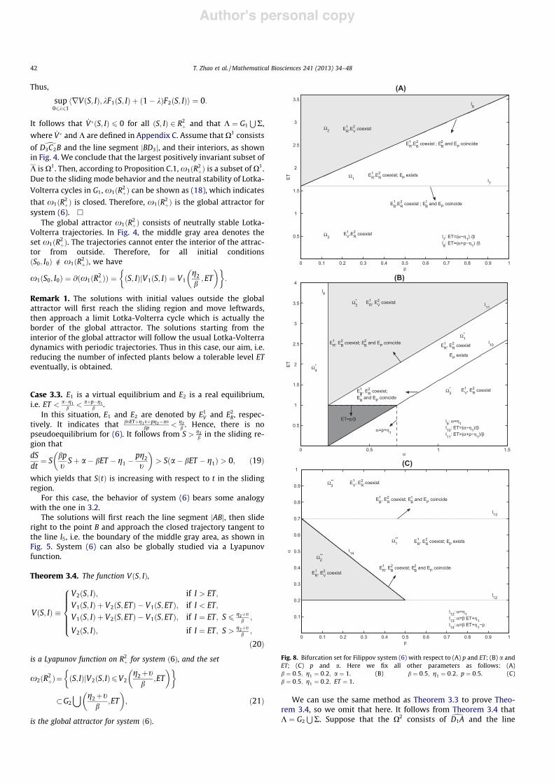
Fig. 8. Bifurcation set for Filippov system (6) with respect to (A) p and ET; (B) a andET; (C) p and a. Here we fix all other parameters as follows: (A)b # 0:5; g1 # 0:2; a # 1. (B) b # 0:5; g1 # 0:2; p # 0:5. (C)b # 0:5; g1 # 0:2; ET # 1.



segment jAD1j and their interiors in Fig. 5. Then the largest posi-tively invariant subset of K is X2. According to Proposition C.1,x2!R2

%" is a subset of X2 and can be written as (21), which

demonstrates that x2!R2%" is closed. In Fig. 5, the middle gray area

denotes the set x2!R2%". For the initial point satisfying

!S0; I0" R x2!R2%", it is easy to see that

0 1 2 3 4 5 6 7 8 9 10

1

2

3

4

5

6

7

S

I

(A)

L5

L4

L3

L1 L2

A1

A2

ER

EP

A4 A5 A6

A7

A8

A9

!2

!1

L1: S="2/#L2: S=("2+$)/#L3: I=(p!"1)/#L4: I=ETL5: I=I0

A3

0 1 2 3 4 5 6 7

0.5

1

1.5

2

2.5

3

3.5

4

4.5

5

S

I

(B)

L4

L3

L5

L1 L2

A1 A2

A3A5

A9

A8

EV!1

L1: S="2/#L2: S=("2+$)/#L3:S=(p!"1)/#L4: I=ETL5: I=I0

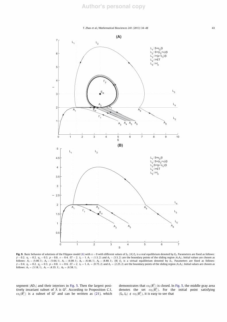
Fig. 9. Basic behavior of solutions of the Filippov model (6) with a # 0 with different values of S0. (A) E2 is a real equilibrium denoted by ER . Parameters are fixed as follows:b # 0:2; g1 # 0:2; g2 # 0:3; p # 0:8; t # 0:4; ET # 2; I0 # 1. A1 # !1:5;2" and A2 # !3:5;2" are the boundary points of the sliding region jA1A2j. Initial values are chosen asfollows: A3 # !5:00;1"; A4 # !5:64;1"; A5 # !6:00;1"; A6 # !6:44;1"; A8 # !8:88;1". (B) E2 is a virtual equilibrium denoted by EV . Parameters are fixed as follows:b # 0:4; g1 # 0:2; g2 # 0:3; p # 0:8; t # 0:6; ET # 2; I0 # 1. A1 # !0:75;2" and A2 # !2:25;2" are the boundary points of the sliding region jA1A2j. Initial values are chosen asfollows: A3 # !3:18;1"; A5 # !4:35;1"; A8 # !6:58;1".



x2!S0; I0" # @!x2!R2%"" # !S; I"jV2!S; I" # V2

g2 % tb

; ET" #! $

:

Remark 2. Any trajectory initiating from the outside of the setx2!R2

%" will approach the @!x2!R2%"" eventually. Any trajectory

starting from the interior of x2!R2%" will follow the dynamics of

system (8) and hence exhibit periodic oscillation. Note that, in thiscase, the eventual number of infected plants is larger than or equalto the ET, which is not our desire, since this will cause greateconomic losses. Therefore, in practice, we would like to avoid thissituation.

Case 3.4. E1 is a real equilibrium and E2 is a boundary equilibrium,i.e. ET # a%p$g1

b .For this situation, we denote E1 as E1

R and E2 as E2B. It is easy to

see that eS2 # g2%tb . Thus, EP and E2

B coincide at the point

B # g2%tb ; ET

% &and l4 coincides with l5, as shown in Fig. 6. Compar-

ing Fig. 6 and Fig. 4, we see that the dynamics of Filippov system(6) in 3.4 is similar to 3.2. Therefore, there exists a global attractor

x1!R2%" given by (18), which consists of dC1AC1 and its interior. The

middle gray area in Fig. 6 denotes the x1!R2%".

Case 3.5. E1 is a boundary equilibrium and E2 is a real equilibrium,i.e. ET # a$g1

b .

In this case, we denote E1 as E1B and E2 as E2

R. It is easy to yieldeS2 # g2

b . EP and E1B coincide at the point A # g2

b ; ET% &

and l3 coincides

with l5, as shown in Fig. 7. It follows from Fig. 7 and Fig. 5 that thesolutions of Filippov system (6) in 3.5 and 3.3 have the analogousdynamical behavior. Therefore, the global attractor x2!R2

%" existsand can be expressed by (21), which consists of the trajectorygoing through the point B and tangent to the line l5 and its interior.In Fig. 7, the middle gray area denotes the set x2!R2

%".So far, the global dynamics of the Filippov plant disease system

(6) have been investigated and the main results obtained above aresummarized in Table 1. For the result (I), our control object — thatis, ensuring the number of infected plants does not exceed the ETeventually — can be reached under some conditions for the initialvalues. For the result (II), our goal can be achieved, while for theresult (III) our target fails to be reached.

3.3. The effects of parameters on dynamics of system (6)

It follows from the above global analysis that a and p are twofactors in determining the dynamics of the system (6). To addressthe richness of the possible equilibria of (6), we let parameters pand ET vary and fix other parameters to build the bifurcation dia-gram, as shown in Fig. 8A. Define

l7 # !p; ET"jET # a$ g1

b

! $; l8 # !p; ET"jET # a% p$ g1

b

! $:

The lines l7 and l8 divide the p-ET parameter space into three re-gions, X1;X2 and X3, and the existence of various types of equilibriais indicated in each region. The ranges of parameters in Cases 3.1,3.2, 3.3, 3.4 and 3.5 correspond to X1;X2;X3, l8 and l7, respectively.As a result of the previous discussion, it is clear that the gray area ofFig. 8A, which consists of X2 and l8, is the region in which our goal ofcontrolling plant diseases can always be achieved. If parameters areselected from X1, the goal may be reached depending on the initialnumbers of both plants. The number of infected plants is alwaysmore than the given ET if the parameters are set in X3 or l7; how-ever, this is not what we pursue. All in all, if other parameters arefixed and the given ET is relatively small, i.e. less than or equal to

a$g1b , then no matter what the value of p is, we cannot reach the tar-

get since the number of infected plants is greater than the ET even-tually. If the ET is relatively large, i.e. greater than a$g1

b , then ourobjective can always be achieved provided 0 < p 6 bET % g1 $ a,and may be reached in some cases provided p > bET % g1 $ a,depending on the initial conditions. Therefore, if we adjust thereplanting rate for the susceptible plants p to control the plant dis-eases, then the number of infected plants will not be less than thethreshold finally unless the threshold ET is relatively large.

Next, we let parameters a and ET change and fix other parame-ters to build the bifurcation diagram, as shown in Fig. 8B. Define

l9 # !a; ET"ja # g1f g; l10 # !a; ET"jET # a$ g1

b

! $;

l11 # !a; ET"jET # a% p$ g1

b

! $:

Here, suppose p > g1. The lines l9; l10 and l11 divide the a-ET param-eter space into four regions, X(i , with i # 1;2;3;4. Since a < g1 in X(4,our above discussions focus on R2

% nX(4. The ranges of parameters inCases 3.1, 3.2, 3.3, 3.4 and 3.5 correspond to X(1, X(2;X

(3; l11 and l10,

respectively. The middle gray area consists of X(2 and l11, in whichour aim is always achieved. For a smaller threshold, i.e. ET less thanor equal to p=b, we can choose the parameters in the dark gray areain X(1, so that the goal may be reached, depending on the initial val-ues of both plants. For a larger threshold, i.e. ET greater than p=b,the parameters can be chosen in X(1 with appropriate initial condi-tions or in the middle gray area so that the number of infectedplants can be maintained below ET eventually. For the case ofp 6 g1, we will get similar conclusions.

From the above analysis, it is natural to ask how the parametersp and a jointly affect the dynamic behavior of system (6) if ET isfixed. We use Fig. 8C to address this. Define

l12 # !p;a"ja # g1f g; l13 # !p;a"ja # bET % g1f g; l14

# !p;a"ja # bET % g1 $ pf g:

The above three lines divide the parameter space into four parts. Be-cause a > g1 holds in our discussions, we consider the issue inX((i ; i # 1;2;3; l13 and l14. The conditions a < bET % g1 anda% p > bET % g1, corresponding to Case 3.1, are valid in X((1 . Theranges of a P bET % g1; a% p > bET % g1, corresponding to Cases3.3 and 3.5, are satisfied in X((3 and l13; the ranges of a < bET % g1and a% p 6 bET % g1, corresponding to Cases 3.2 and 3.4, hold truein X((2 and l14. From these correspondences, we conclude the follow-ing results. First, suppose the planting rate a is relatively small, i.e.less than bET % g1. If the replanting rate p is so small that theparameters belong to the gray area — that is, the conditiona% p 6 bET % g1 holds — then the number of infected plants can al-ways be eventually reduced below the threshold. If p is relativelylarge so that a% p > bET % g1, i.e. !a;p" 2 X((1 , then the objective isachieved by choosing the initial number of plants to satisfy the con-dition that S0 2 D, where D # !SC4k%1 ; SC4k%2 "

S!SC4k%4 ; SC4k%5 "; k P 0, as

shown in (14). Secondly, assume a is relatively large, i.e. greater

Table 2Main results of model (6) with a # 0.

Tapes of E2 Conditions Existence of pseudoequilibrium Main results

ER ET < p$g1b

Yes (i)

EV ET > p$g1b

No (ii)

EB ET # p$g1b

EP and EB coincide (ii)

The subscript of E, i.e. R, V or B, denotes the type of E2 is real, virtual or boundaryequilibrium, respectively. EP is the pseudoequilibrium of (6). (i) means that bothplants either tend to C2 or go to the origin eventually, depending on initial values.(ii) denotes both plants approach extinction.



than or equal to bET % g1. Then, no matter what the value of p is, thenumber of infected plants will eventually exceed the threshold, soour target fails to be achieved. Therefore, the dynamic behavior of(6) can be determined by the planting and replanting rates. Theabove information can guide our production practices.

Remark 3. By using similar analysis as Subsection , we could getthe main results for the special system (6) with null-planting rate(a # 0). Note that the null-planting rate has been considered byTang et al. in the model with ET [18].

Case 3.1 corresponds to the situation where E2 is a real equilib-rium denoted by ER, i.e. ET < p$g1

b . The stable origin with a # 0 cor-responds to E1 with a > 0, for the model !7". For any given ET, thereis a phase trajectory of model (7) denoted by C1, starting from thepoint A3 on L5 (L5 : I # I0), tangent to the line L4 (L4 : I # ET), at thepoint A1 # !g2=b; ET". There also exists a closed trajectory of themodel (8), denoted by C2, that is tangent to L4 at A2 # !g2%t

b ; ET",as shown in Fig. 9A. The trajectory starting from a point on L5 withSA3 < S0 < SA8 will enter the sliding region jA1A2j with the pseudo-equilibrium EP . However, only the solutions in the middle grayarea, which start from the segment jA4A6j, approach the closed tra-jectory C2 eventually; others will eventually approach !0;0".

Case 3.2 corresponds to the situation where E2 is a virtual equi-librium denoted by EV , i.e. ET > p$g1

b . The trajectories with initialvalues satisfying SA3 < S0 < SA8 will experience sliding motion. Allsolutions starting from any point on the line L5 will tend to the ori-gin, which reveals that both susceptible and infected plants witharbitrary initial numbers always go to extinction, as shown inFig. 9B.

Case 3.4 corresponds to the situation where E2 is a boundaryequilibrium denoted by EB, i.e. ET # p$g1

b . We note that the dynam-ics of (6) in this case are similar to the above situation. Therefore,all the solutions starting from any point on the line L5 will eventu-ally tend to zero. In addition, Cases 3.3 and 3.5 do not exist underthe condition a # 0.

The main results obtained here are displayed in Table 2, whichdemonstrates that the numbers of susceptible and infected plantseither go to zero or oscillate periodically with I P ET . Therefore,in this scenario of null-planting rate, we fail to control plantdiseases.

4. Biological conclusions and discussion

Recently, the Filippov system has attracted great attention indifferent fields, since it provides a natural and rational frameworkfor many real-world problems. The threshold policy has beenwidely used in grazing, harvesting and culling [25,30,31]. In partic-ular, in the scenario of controlling plant disease, the plants are ro-gued and replanted only when the number of infected plantsreaches or exceeds the ET. The main purpose of this paper is touse the Filippov system to model this intervention and examinethe conditions under which the number of infected plants is even-tually maintained below the ET while ensuring susceptible plantsdo not become extinct. Therefore, the Filippov plant disease mod-els developed here describe the disease dynamics associated withcultural strategy and threshold policy. Making use of the qualita-tive analysis of the global dynamics of the model, we have estab-lished conditions under which our objective can be achieved,which are summarized in Table 1.

It is worth noting that the Filippov models described here differfrom the state-dependent impulsive differential models discussedby Tang et al. [18] and have many advantages from the point ofview of plant disease management and mathematics, although nei-ther system is smooth. First, the trajectories of impulsive modelsare not continuous, while the trajectories of the Filippov systemsproceeding along alternate subsystems are continuous. Secondly,under the state-dependent impulsive modeling approach, theinterventions are implemented instantaneously; conversely, inthe Filippov systems, when the number of infected plants reachesor exceeds the ET, control measures are triggered, the system is

0 0.5 1 1.5 2 2.5 30

0.5

1

1.5

2

2.5

3

3.5

4

S

I

ER2

ER1

A1

A2A3

l4

l5

l1 , l2

l3l6


Fig. 10. Basic behavior of the solution of the Filippov model (6) with t # 0 when E1 and E2 are real equilibria denoted by E1R and E2

R , respectively. Parameters are fixed asfollows: b # 0:5;g1 # 0:2;g2 # 0:4;p # 0:6; ET # 1:2;a # 0:5. Initial value is taken as follows A1 # !S0; I0" # !2;0:4".



switched into the control system, and interventions last for a dura-tion until to the next switch. Hence, non-instantaneous control ismodeled in the Filippov systems. Thirdly, the Filippov systemscan give rise to qualitatively new behavior, such as the appear-ances of various types of equilibria and sliding dynamics. There-fore, it is more meaningful and realistic to use Filippov systemsto investigate the development of plant diseases. However, thesliding nature of the Filippov systems makes the study morecomplicated.

It should be emphasized that, by making full use of the firstintegral, Lambert W Function and Lyapunov function, we haveexamined the global dynamics for model (6) with proportionalplanting rate: the nonexistence of a limit cycle and the existenceof a global attractor. The methods used here can be applied to com-pletely analyze many Lotka-Volterra models with first integrals,such as a predation model proposed by Krivan [32]. However, thereare limitations for some nonlinear systems without the first inte-grals. That is because, with the help of analytical solutions or firstintegrals, we could easily get the trajectories in the phase planeand investigate the global dynamics. The analysis of Section 3 re-veals that there does not exist the limit cycle in G1

SG2, and the

global attractor of Case 3.1, 3.2, 3.3, 3.4, 3.5 refers to C1SC2 andits interior, x1!R2

%";x2!R2%", x1!R2

%";x2!R2%", respectively.

The planting and replanting rates are two important factors indetermining the dynamical behavior of the system. First, if only pchanges among parameters of (6), then our objective can bereached provided the ET is relatively large (i.e. ET > a$g1

b ) and oneof the following conditions holds: (i) 0 < p 6 bET % g1 $ a; (ii)p > bET % g1 $ a; S0 2 D, where D # !SC4k%1 ; SC4k%2 "

S!SC4k%4 ; SC4k%5 ";

k P 0. Secondly, let a change and a > g1; p > g1 be valid. Whenthe ET is relatively small (i.e. ET 6 p=b), we can achieve the targetif we control the parameter a to satisfy bET % g1 $ p < a < bET%g1; S0 2 D. When the ET is relatively large (i.e. ET > p=b), we canachieve the target if one of the following conditions holds true:(i) a 6 bET % g1 $ p, (ii) bET % g1 $ p < a < bET % g1; S0 2 D.Thirdly, if the ET is fixed, and p and a vary, the goal can be achievedif the parameters satisfy one of the conditions as follows:

(i) a < bET % g1; a% p 6 bET % g1;(ii) a < bET % g1; a% p > bET % g1; S0 2 D.Consequently, we can use the initial conditions, the planting

and replanting rates to design the threshold policy such that thenumber of infected plants can be maintained below the ETeventually.

It is always postulated that t > 0; p > 0 in the Filippov plantdisease model (6), which indicates that the replanting and roguingcontrol strategies are implemented simultaneously. What is the re-sult if we only carry out one control? First, assume t # 0; p > 0.Here, we take the case that E1 and E2 are real equilibria as an exam-ple. It follows from Fig. 10 that the trajectory starting from A1 isclosed. These reveal that all trajectories are closed, which gives dif-ferent dynamic behavior compared with t > 0; p > 0. For othercases, we will get similar results. Hence, if we only carry outreplanting control when I > ET, the goal cannot be achieved.Secondly, suppose t > 0; p # 0. The sliding-mode dynamics aredescribed by

dS!t"dt# !a$ bET $ g1"S!t": !22"

There are three situations: 1. E1R and E2

V ; 2. E1V and E2

R; 3. E1B and E2

B.The results of the first two situations are the same as those in Cases3.2 and 3.3, respectively. However, for the third situation, accordingto (22) and a$g1

b # ET , we have dS=dt # 0 in the sliding region R1, soall points in R1 are pseudoequilibria for (6). Making use of qualita-tive analysis, it is easy to see that all solutions will eventually sta-bilize at a point in R1, which is a new phenomenon comparedwith t > 0; p > 0. So we can reach the target in this case. To sum

up, if we only implement replanting control, we will fail to achieveour aim. If we only carry out roguing control, our aim may beachieved.

We mention that we here consider the effort to replant or rogueplants to be proportional to the number of plants. This assumptioncould be initially reasonable from the point of view of mathematics[18]. That is because the proportional roguing cannot lead to neg-ative solutions compared to the relatively large constant roguing.Moreover, the values of the proportional roguing and replantingrates might depend on the availability of workers. Our results indi-cate that we may not reach our goal mentioned above if the ratesare not appropriate. It is interesting to note that the replanting androguing plants can be modeled by constants, independent of theexisting numbers of plants or the number of available workers.We leave this for future work.

The related practical significance for all results obtained in thiswork can guide us to establish a good treatment program and pre-vent an intolerable build-up of diseases. Finally, it is essential tolink the costs of implementing controls to modeling of plant dis-ease epidemics, to consider other strategies of IDM, such as biolog-ical tactics that introduce some natural enemies of the insects whotransmit plant diseases in the plant-growth environment. We leavethese for further investigations.

Acknowledgements

Research was supported by the National Natural Science Foun-dation of China (NSFC 11171268), by the Fundamental ResearchFunds for the Central Universities (08143042), and by the Interna-tional Development Research Center, Ottawa, Canada (104519-010). R.J.S.? was supported by an NSERC Discovery Grant, an EarlyResearcher Award and funding from MITACS. For citation purposes,note that the question mark is part of his name.

Appendix A. Methods for analyzing sliding solution

Filippov convex method: The Filippov method associates the fol-lowing convex combination M1!X" of the two vectors F1!X" andF2!X" to each nonsingular sliding point X 2 R1, i.e.

M1!X" # kF1!X" % !1$ k"F2!X";

where k # hHX !X";F2!X"ihHX !X";F2!X"$F1!X"i

. M1!X" is tangent to R1.

Thus, the sliding-mode dynamics can be determined by

dX!t"dt# M1!X!t""; X 2 R1; !A:1"

which is smooth on a one-dimensional sliding interval of R1. Thesolution of (A.1) is the sliding solution.

Utkin equivalent control method: Utkin proposed an equivalentcontrol method to describe the sliding-mode dynamics on theswitching line R for (2). Assume that a sliding mode exists on R,i.e. R1 is non-empty. The Filippov system (2) can be rewritten as

dX!t"dt# M2!X;lH"; !A:2"

where the control lH is defined as

lH #0; if H!X" < 0;l; if H!X" > 0;

!!A:3"

with l a continuous function.The solution of the equation

dH!t"dt# @H@X

M2!X;lH" # 0 !A:4"

with respect to lH is referred to as ‘‘equivalent control’’. We denoteit by l(H . Substituting lH with l(H yields



dX!t"dt# M2!X;l(H"; X 2 R1; !A:5"

which determines the sliding-mode dynamics of the Filippov sys-tem (2).

Appendix B. Definitions of Lambert W function and equilibrium

Definition 4.1. [28] The Lambert W function is defined to be themulti-valued inverse of the function z! zez satisfying

LambertW!z" exp!LambertW!z"" # z:

It is easy to see that the function zez has the positive derivative!z% 1" exp!z" if z > $1. The inverse function of zez restricted onthe interval +$1;1, is defined by LambertW!0; z". For simplicity,LambertW!0; z" ) LambertW!z". Similarly, we define the inversefunction of zez restricted on the interval !$1;$1, to beLambertW!$1; z". Now we define the concepts of various types ofequilibria for system (2).

Definition 4.2.

(i) A point E is called a real equilibrium of (2) if

F1!E" # 0; H!E" < 0; or F2!E" # 0; H!E" > 0:

A point E is called a virtual equilibrium of (2) if

F1!E" # 0; H!E" > 0; or F2!E" # 0; H!E" < 0:

(ii) A point E is called a pseudoequilibrium if it is an equilibriumof the sliding mode (A.1) or (A.5), i.e.

M1!E" # 0; H!E" # 0; or M2!E" # 0; H!E" # 0:

(iii) A point E is called a boundary equilibrium of (2) if

F1!E" # 0; H!E" # 0; or F2!E" # 0; H!E" # 0:

It follows from the above definitions that a stable virtual equilib-rium is never actually attained since the dynamic change as soonas the trajectory crosses the switching manifold R.

Appendix C. Definition of Lyapunov function and theories onthe global quality of the Filippov system

Denote the solution from a given initial condition X0 of (2) byuX0

, the x limit set by x!X0" and, for G & R2%,

AG!t" ) fX 2 R2%jX # uX0

!t" for some X0 2 Gg; n!G" )[

tP0

AG!t":

Definition 4.3. [29] A function V 2 C1!R2%" is called a Lyapunov

function of (2) on G & R2% if it is nonnegative on G and, for all X 2 G,

_V(!X" ) maxj2F!X"

hrV!X";ji 6 0;

where F!X" is defined as follows:

F!X" )fF1!X"g; if X 2 G1;

fkF1!S; ET" % !1$ k"F2!S; ET" : k 2 +0;1,g; if X 2 R;fF2!X"g; if X 2 G2:

8><

>:

!C:1"

Proposition 4.1. [29] (LaSalle’s Invariance Principle) Suppose thatG & R2

% is an open set which satisfies x!G" )S

x2Gx!X" & n!G". Let

every Filippov solution uX0; X0 2 G, of (2) be unique and defined for

all t P 0, and V : R2% ! R be a Lyapunov function of (2) on n!G". Then

x!G" is a subset of the largest positively invariant subset of K, whereK ) fX 2 Gj _V(!X" # 0g.

Corollary 4.1. [29] Assume that G and V : R2% ! R satisfy Proposition

C.1 and R2% n G is repelling, in the sense that all solutions stay in R2

% n G

for only a finite time. Let x!R2%" # x!G" be bounded. Then x!R2

%" isglobally asymptotically stable.

Appendix D. The proof of Theorem 3.1

Proof. If k # 1, according to (12) it is easy to illustrate that (14)holds. Assume that (14) holds true for k # N, i.e.

SC4N%2 # UN$13 U1!eS2"; SC4N%3 # UN$1

3 U1g2 % t

b

" #;

SC4N%4 # UN$13 U2!eS2"; SC4N%5 # UN$1

3 U2g2

b

" #:

!D:1"

If k # N % 1, then the paths of the corresponding critical trajectoriescan be shown as follows:

(I) !4N%5N%1;N%1 : C4N%6 ! D4N%6 ! E4N%1 ! C4N%2;

(II) !4N%6N%1;N%1 : C4N%7 ! D4N%7 ! E4N%2 ! C4N%3;

(III) !4N%7N%1;N%2 : C4N%8 ! D4N%8 ! E4N%3 ! C4N%4;

(IV) !4N%8N%1;N%2 : C4N%9 ! D4N%9 ! E4N%4 ! C4N%5,

where C4N%2;C4N%3;C4N%4;C4N%5 are the initial points of the criticaltrajectories !4N%1

N;N ;!4N%2N;N ;!4N%3

N;N%1 and !4N%4N;N%1, respectively. Due to

the results (D.1) and the facts that

SE4N%1 # W1!SC4N%2 "; SD4N%6 # W2!SE4N%1 "; SC4N%6 # W3!SD4N%6 ";

we have

SC4N%6 # W3 *W2 *W1!SC4N%2 " # U3!SC4N%2 " # U3 *UN$13 U1!eS2"

# UN3 U1!eS2":

Using the same method, we get the following conclusions

SC4N%7 # UN3 U1

g2 % tb

" #; SC4N%8 # UN

3 U2!eS2";

SC4N%9 # UN3 U2

g2

b

" #:

Therefore, the conclusion (14) is true for k # N % 1, which demon-strates that (14) holds true for all positive integers k. h

References

[1] R.W. Gibson, J.P. Legg, G.W. Otim-Nape, Unusually severe symptoms are acharacteristic of the current epidemic of mosaic virus disease of cassava inUganda, Ann. Appl. Biol. 128 (1996) 479.

[2] T. Iljon, J. Stirling, R.J. Smith?, A mathematical model describing an outbreak ofFire Blight, in: S. Mushayabasa, C.P. Bhunu (Eds.), Understanding the Dynamicsof Emerging and Re-emerging Infectious Diseases Using Mathematical Models,2012, pp 91–104.

[3] L.M.C. Medina, I.T. Pacheco, R.G.G. Gonzalez, et al., Mathematical modelingtendencies in plant pathology, Afr. J. Biotechnol. 8 (2009) 7399.

[4] R.A.C. Jones, Determining threshold levels for seed-borne virus infection inseed stocks, Virus Res. 71 (2000) 171.

[5] R.A.C. Jones, Using epidemiological information to develop effective integratedvirus disease management strategies, Virus Res. 100 (2004) 5.

[6] T.T. Zhao, S.Y. Tang, Plant disease control with economic threshold, J. Biomater.24 (2009) 385.

[7] H.R. Thieme, J.A.P. Heesterbeek, How to estimate the efficacy of periodiccontrol of an infectious plant disease, Math. Biosci. 93 (1989) 15.

[8] F. van den Bosch, N. McRoberts, F. van den Berg, L.V. Madden, The basicreproduction number of plant pathogens: matrix approaches to complexdynamics, Phytopathology 98 (2008) 239.



[9] F. van den Bosch, M.J. Jeger, C.A. Gilligan, Disease control and its selection fordamaging plant virus strains in vegetatively propagated staple food crops; atheoretical assessment, Proc. R. Soc. B 274 (2007) 11.

[10] F. van den Bosch, A.M. Roos, The dynamics of infectious diseases in orchardswith roguing and replanting as control strategy, J. Math. Biol. 35 (1996) 129.

[11] M.S. Chan, M.J. Jeger, An analytical model of plant virus disease dynamics withroguing, J. Appl. Ecol. 31 (1994) 413.

[12] J.C. Zadoks, R.D. Schein, Epidemiology and Plant Disease Management, OxfordUniversity, New York, 1979.

[13] L.V. Madden, G. Hughes, F. van den Bosch, The Study of Plant DiseaseEpidemics, The American Phytopathological Society, St. Paul, Minnesota, USA,2007.

[14] S. Fishman, R. Marcus, H. Talpaz, et al., Epidemiological and economic modelsfor the spread and control of citrus tristeza virus disease, Phytoparasitica 11(1983) 39.

[15] V. Capasso, Mathematical Structures of Epidemic Systems, Springer-Verlag,Berlin, 1993.

[16] S.Y. Tang, Y.N. Xiao, R.A. Cheke, Multiple attractors of host-parasitoid modelswith integrated pest management strategies: eradication, persistence andoutbreak, Theor. Popul. Biol. 73 (2008) 181.

[17] S.Y. Tang, R.A. Cheke, Models for integrated pest control and their biologicalimplications, Math. Biosci. 215 (2008) 115.

[18] S.Y. Tang, Y.N. Xiao, R.A. Cheke, Dynamical analysis of plant disease modelswith cultural control strategies and economic thresholds, Math. Comput.Simul. 80 (2010) 894.

[19] A.F. Filippov, Differential Equations with Discontinuous Righthand Sides,Kluwer Academic, Dordrecht, 1988.

[20] V.I. Utkin, Sliding Modes in Control and Optimization, Springer, Berlin, 1992.[21] V.I. Utkin, J. Guldner, J.X. Shi, Sliding Mode Control in Electro-mechanical

Systems, second ed., Taylor & Francis Group, 2009.[22] M.D. Bernardo, C.J. Budd, A.R. Champneys, et al., Bifurcations in nonsmooth

dynamical system, SIAM Rev. 50 (2008) 629.[23] B. Brogliato, Nonsmooth Mechanics, Springer-Verlag, NY, 1999.[24] M.I.S. Costa, Harvesting induced fluctuations: insights from a threshold

management policy, Math. Biosci. 205 (2007) 77.[25] M.I.S. Costa, E. Kaszkurewicz, A. Bhaya, L. Hsu, Achieving global convergence to

an equilibrium population in predator–prey systems by the use of adiscontinuous harvesting policy, Ecol. Model. 128 (2000) 88.

[26] F. Dercole, A. Gragnani, S. Rinaldi, Bifurcation analysis of piecewise smoothecological models, Theor. Popul. Biol. 72 (2007) 197.

[27] M. di Bernardo, P. Kowalczyk, A. Nordmark, Bifurcation of dynamical systemswith silding: derivation of normal-form mappings, Physica D 170 (2002) 175.

[28] R.M. Corless, G.H. Gonnet, D.E.G. Hare, et al., On the Lambert W function, Adv.Comput. Math. 5 (1996) 329.

[29] D.S. Boukal, V. Krivan, Lyapunov functions for Lotka–Volterra predator-preymodels with optimal forging behavior, J. Math. Biol. 39 (1999) 493.

[30] M.I.S. Costa, L.D.B. Faria, Integrated pest management: theoretical insightsfrom a threshold policy, Neotrop. Entomol. 39 (2010) 1.

[31] M.E.M. Meza, A. Bhaya, E. Kaszkurewicz, M.I.da S. Costa, Threshold policiescontrol for predator–prey systems using a control Liapunov function approach,Theor. Popul. Biol. 67 (2005) 273–284.

[32] V. Krivan, Effects of optimal antipredator behavior of prey on predator–preydynamics: the role of refuges, Theor. Popul. Biol. 53 (1998) 131.


author's personal copy - university of...

Documents