1

The Impact of Temperature on Mortality in Tianjin, China: A Case−crossover Design with A

Distributed Lag Non-linear Model

Authors' full name and affiliations:

Yuming Guo1*

, Adrian G Barnett1, Xiaochuan Pan

2, Weiwei Yu

1, Shilu Tong

1

1 School of Public Health and Institute of Health and Biomedical Innovation, Queensland

University of Technology, Brisbane, Australia.

2 School of Public Health, Peking University, Beijing, China.

Corresponding author’s name and complete contact information:

Yuming Guo: School of Public Health, Queensland University of Technology, Kelvin Grove,

Brisbane, Queensland 4059, Australia; Tel: +61 7 31383996; Fax: +61 7 31383130; Email

address: guoyuming@yahoo.cn;

Running head: Case−crossover on Non-linear Temperature Effect

Key words: Cardiovascular mortality; Case−crossover; Distributed lag non-linear model;

Mortality; Respiratory mortality; Temperature

Acknowledgements: We thank the Tianjin Municipal Environmental Monitoring Center for

providing air pollution data, China Meteorological Data Sharing Service System for

providing meteorology data, and Chinese Centre for Disease Control and Prevention for

providing mortality data.

2

Grant information: This study is funded by the National Natural Science Foundation of

China (#30972433); Y.G. is supported by the QUT Postgraduate Research Award

(QUTPRA); S.T is supported by a NHMRC Research Fellowship (#553043).

Conflict of interest: None

Abbreviations

AIC: Akaike information criterion; CI: confidence interval; DLNM: distributed lag non-linear

model; ICD: International Classification of Diseases; NO2: nitrogen dioxide; PM10:

particulate matter with aerodynamic diameters less than 10 µm; SO2: sulphur dioxide

3

Abstract

Background: There has been increasing interest in assessing the impacts of temperature on

mortality. However, few studies have used a case–crossover design to examine non-linear

and distributed lag effects of temperature on mortality. Additionally, little evidence is

available on the temperature-mortality relationship in China, or what temperature measure is

the best predictor of mortality.

Objectives: To use a distributed lag non-linear model (DLNM) as a part of case–crossover

design. To examine the non-linear and distributed lag effects of temperature on mortality in

Tianjin, China. To explore which temperature measure is the best predictor of mortality;

Methods: The DLNM was applied to a case−crossover design to assess the non-linear and

delayed effects of temperatures (maximum, mean and minimum) on deaths (non-accidental,

cardiopulmonary, cardiovascular and respiratory).

Results: A U-shaped relationship was consistently found between temperature and mortality.

Cold effects (significantly increased mortality associated with low temperatures) were

delayed by 3 days, and persisted for 10 days. Hot effects (significantly increased mortality

associated with high temperatures) were acute and lasted for three days, and were followed

by mortality displacement for non-accidental, cardiopulmonary, and cardiovascular deaths.

Mean temperature was a better predictor of mortality (based on model fit) than maximum or

minimum temperature.

Conclusions: In Tianjin, extreme cold and hot temperatures increased the risk of mortality.

Results suggest that the effects of cold last longer than the effects of heat. It is possible to

combine the case−crossover design with DLNMs. This allows the case−crossover design to

flexibly estimate the non-linear and delayed effects of temperature (or air pollution) whilst

controlling for season.

4

Introduction

Heat-related mortality has become a matter of increasing public health significance,

especially in the light of climate change. Studies have examined hot and cold temperatures in

relation to total non-accidental deaths and cause-specific deaths (Stafoggia et al. 2006). The

city- or region-specific temperature-mortality relationship is often V-, U- or J-shaped, with

increases in mortality at temperatures below (above) the cold (hot) threshold (Hajat and

Kosatky 2010). The temperature-mortality relationship varies greatly by geographic, climate

and population characteristics (Group 1997). Social, economic, demographic and

infrastructure factors can influence the sensitivity of populations to temperature (Ebi et al.

2006). In China, only a few studies on temperature-mortality relationship have been

conducted in Shanghai (Kan et al. 2003), Hong Kong (Chan et al. 2010) and Beijing (Liu et al.

2011). No research has been undertaken in Tianjin, one of the largest cities in northeastern

China.

A previous study found that no temperature measure (maximum, mean or minimum

temperature) was consistently better at predicting mortality in the US. The best temperature

measure differed by age group, season and region (Barnett et al. 2010). It is unknown which

temperature measure is the best predictor of mortality in Tianjin.

Mortality risk depends not only on exposure to the current day’s temperature, but also on

several previous days’ exposure (Anderson and Bell 2009). The distributed lag model has

been applied to explore the delayed effect of temperature on mortality (Analitis et al. 2008;

Baccini et al. 2008; Hajat et al. 2005). To overcome the strong correlation between daily

temperatures over short time periods, constrained distributed lag structures are used in time

5

series regressions (Armstrong 2006). The estimates are constrained by smoothing using

methods such as natural cubic splines, polynomials, or stratified lag. Both unconstrained and

constrained distributed lag models assume a linear relationship between temperature below

(above) the cold (hot) threshold and mortality, so these models may not be sufficiently

flexible to capture the effects of temperature on mortality.

Recently, a distributed lag non-linear model (DLNM) was developed to simultaneously

estimate the non-linear and delayed effects of temperature (or air pollution) on mortality (or

morbidity) (Armstrong 2006; Gasparrini et al. 2010). DLNMs use a “cross-basis” function

that describes a two-dimensional temperature-response relationship along the dimensions of

temperature and lag. The choice of “cross-basis” functions for the temperature and lag are

independent, so the spline or linear functions can be used for temperature, while the

polynomial functions can be used for the lag. The estimates can be plotted using a 3-

dimensional graph to show the relative risks along both temperature and lags. We can predict

the relative risks for a certain temperature or lag, by extracting a “slice” from the 3-

dimensional graph. We can compute the overall effect by summing the log relative risks of

each lag. Separate smoothing functions are applied to time in order to control for season and

secular trends.

The case−crossover design controls for seasonal effects and secular trends by matching case

and control days in relatively small time windows (e.g., calendar month). This controls for

season using a step-function rather than a smooth spline function (Barnett and Dobson 2010).

Most previous studies used the case–crossover design with relatively inflexible models to

investigate the effects of temperature on mortality, such as assuming a linear effect for

temperature in each season, with a single lag model, or moving average lag model (Basu et al.

6

2008; Green et al. 2010). Few studies have demonstrated how to fit non-linear and delayed

effects of temperature on mortality within a case–crossover design.

We used DLNMs combined with the case–crossover design, making it possible to fit more

sophisticated estimates of the effects of temperature (or air pollution) using a case–crossover

design. We demonstrated these models here using a motivating example of the temperature-

mortality relationship in Tianjin, China, and also investigated which temperature measure had

the best predictive ability for mortality.

Materials and methods

Data collection

Tianjin is a city in northeastern China, and is adjacent to Beijing and Hebei Province, along

the coast of Bohai Gulf (39° 07' North, 117° 12' East). Tianjin has four distinct seasons, with

cold, windy, dry winters influenced by the vast Siberian anticyclone, and hot, humid

summers due to the monsoon. It is the fifth largest Chinese city in terms of urban land area.

The population in the urban area was 4.2 million in 2005.

Mortality data was obtained from the China Information System for Death Register and

Report of Chinese Centre for Disease Control and Prevention from January 1, 2005 to

December 31, 2007. The mortality data were from six urban districts of Tianjin (Heping,

Hedong, Hexi, Nankai, Hebei and Hongqiao). Non-accidental mortality was classified

according to the International Classification of Diseases, 10th revision (ICD-10: A00–R99)

(World Health Organization 2007). Cardiopulmonary (ICD-10:I00–I99 and ICD-10:J00–J99),

7

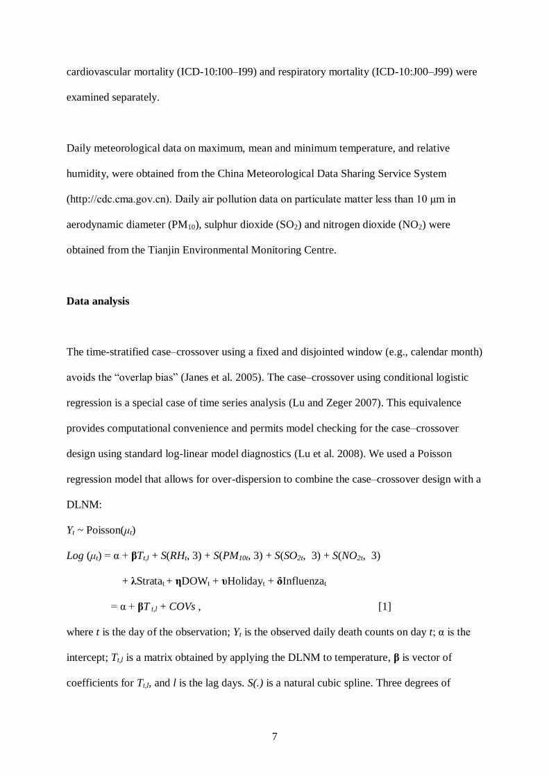
cardiovascular mortality (ICD-10:I00–I99) and respiratory mortality (ICD-10:J00–J99) were

examined separately.

Daily meteorological data on maximum, mean and minimum temperature, and relative

humidity, were obtained from the China Meteorological Data Sharing Service System

(http://cdc.cma.gov.cn). Daily air pollution data on particulate matter less than 10 μm in

aerodynamic diameter (PM10), sulphur dioxide (SO2) and nitrogen dioxide (NO2) were

obtained from the Tianjin Environmental Monitoring Centre.

Data analysis

The time-stratified case–crossover using a fixed and disjointed window (e.g., calendar month)

avoids the “overlap bias” (Janes et al. 2005). The case–crossover using conditional logistic

regression is a special case of time series analysis (Lu and Zeger 2007). This equivalence

provides computational convenience and permits model checking for the case–crossover

design using standard log-linear model diagnostics (Lu et al. 2008). We used a Poisson

regression model that allows for over-dispersion to combine the case–crossover design with a

DLNM:

Yt ~ Poisson(μt)

Log (μt) = α + βTt,l + S(RHt, 3) + S(PM10t, 3) + S(SO2t, 3) + S(NO2t, 3)

+ λStratat + ηDOWt + υHolidayt + δInfluenzat

= α + βT t,l + COVs , [1]

where t is the day of the observation; Yt is the observed daily death counts on day t; α is the

intercept; Tt,l is a matrix obtained by applying the DLNM to temperature, β is vector of

coefficients for Tt,l, and l is the lag days. S(.) is a natural cubic spline. Three degrees of

8

freedom were used to smooth relative humidity, PM10, NO2, and SO2 according to previous

studies (Anderson and Bell 2009; Stafoggia et al. 2008). Stratat is a categorical variable of the

year and calendar month used to control for season and trends, and λ is vector of coefficients.

DOWt is day of the week on day t, and η is vector of coefficients. Holidayt is a binary

variable that is “1” if day t was a holiday. Influenzat is a binary variable that is “1” if there

were any influenza deaths on day t.

Based on the vector of estimated coefficients β in model [1], the DLNM was used to get the

predicted effects and standard errors for combinations of temperature and lags. Graphs,

summaries, and statistical inference can be obtained from the DLNM estimates and standard

errors (Armstrong 2006).

We used a “natural cubic spline-natural cubic spline” DLNM that modelled both the non-

linear temperature effect and the lagged effect using a natural cubic spline. We placed spline

knots at equal spaces in the temperature range to allow enough flexibility in the two ends of

temperature distribution. We placed spline knots at equal intervals in the log scale of lags to

allow more flexible lag effects at shorter delays. To completely capture the overall

temperature effect and adjust for any potential harvesting (heat-related excesses of mortality

were followed by deficits), we used lags up to 27 days according to a previous study

(Armstrong 2006). The median value of temperature was defined as the baseline temperature

(“centering value”) for calculating the relative risks. To choose the degree of freedom (knots)

for temperature and lag, we used Akaike information criterion (AIC) for quasi-Poisson

models (Gasparrini et al. 2010; Peng et al. 2006). We found that 5 degrees of freedom for

temperature and 4 degrees of freedom for lag produced the best model fitting. We plotted the

relative risks against temperature and lags to show the entire relationship between

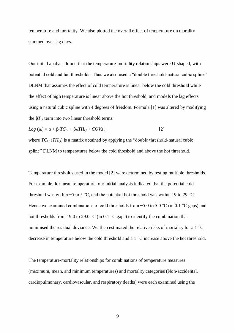
9

temperature and mortality. We also plotted the overall effect of temperature on morality

summed over lag days.

Our initial analysis found that the temperature-mortality relationships were U-shaped, with

potential cold and hot thresholds. Thus we also used a “double threshold-natural cubic spline”

DLNM that assumes the effect of cold temperature is linear below the cold threshold while

the effect of high temperature is linear above the hot threshold, and models the lag effects

using a natural cubic spline with 4 degrees of freedom. Formula [1] was altered by modifying

the βTi,l term into two linear threshold terms:

Log (μt) = α + βcTCt,l + βHTHt,l + COVs , [2]

where TCt,l (THt,l) is a matrix obtained by applying the “double threshold-natural cubic

spline” DLNM to temperatures below the cold threshold and above the hot threshold.

Temperature thresholds used in the model [2] were determined by testing multiple thresholds.

For example, for mean temperature, our initial analysis indicated that the potential cold

threshold was within −5 to 5 °C, and the potential hot threshold was within 19 to 29 °C.

Hence we examined combinations of cold thresholds from −5.0 to 5.0 °C (in 0.1 °C gaps) and

hot thresholds from 19.0 to 29.0 °C (in 0.1 °C gaps) to identify the combination that

minimised the residual deviance. We then estimated the relative risks of mortality for a 1 °C

decrease in temperature below the cold threshold and a 1 °C increase above the hot threshold.

The temperature-mortality relationships for combinations of temperature measures

(maximum, mean, and minimum temperatures) and mortality categories (Non-accidental,

cardiopulmonary, cardiovascular, and respiratory deaths) were each examined using the

10

above steps. The AIC was used to choose the temperature measure that best predicted

mortality.

Sensitivity analyses were performed by changing the window length in the case–crossover

from calendar month to 30, 28 and 21 days to control for season, and varying the maximum

lags to 20 and 30 days for the DLNM.

All statistical tests were two-sided and values of P<0.05 were considered statistically

significant. Spearman’s correlation coefficients were used to summarize the similarities in

daily weather conditions. The R software (version 2.12.1, R Development Core Team 2009)

was used to fit all models, with the “dlnm” package to create the DLNM (Gasparrini and

Armstrong 2011).

A detailed explanation of how to combine the case–crossover with DLNM is provided in the

supplemental material (see Supplemental Material, R code).

Results

The average daily maximum temperature was 19 °C, mean temperature 13 °C, minimum

temperature 8 °C, and relative humidity 60%. On average there were 56 daily non-accidental

deaths, 34 cardiopulmonary deaths, 30 cardiovascular deaths, and 4 respiratory deaths (Table

1). The three temperature measures were strongly correlated (Table 2).

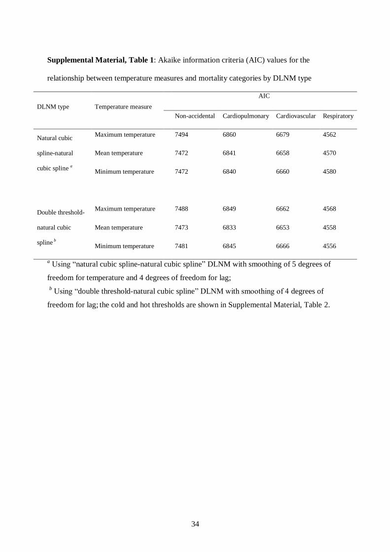
Mean temperature generally gave the lowest AIC values (i.e., had the best predictive ability

for mortality) in Tianjin (see Supplemental Material, Table 1). The “double threshold-natural

11

cubic spline” DLNM generally fit the data better than the “natural cubic spline-natural cubic

spline” DLNM (see Supplemental Material, Table 1). Therefore we report results for

associations with mean temperature only.

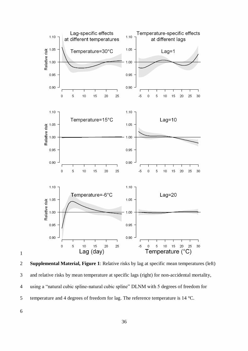
The 3-dimensional plots show the entire surface between mean temperature and mortality

categories at all lag days (Figure 1). The estimated effects of temperature were non-linear for

all mortality types, with higher relative risks at hot and cold temperatures. For example,

extreme hot temperature (30 °C) was positively associated with non-accidental mortality on

current day, whilst extreme cold temperature (–6 °C) significantly increased non-accidental

mortality after 3-days lag. Neither hot effects (i.e., significant increases in mortality

associated with hot temperatures) nor cold effects (i.e., significant increases in mortality

associated with cold temperatures) were apparent after a 20-day lag, with relative risks close

to one across the entire range of temperatures (see Supplemental Material, Figure 1).

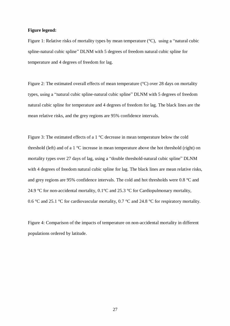
Figure 2 shows the estimated effect of mean temperature over 28 days on mortality. There

were U-shaped relationships between mean temperature and all mortality types, with large

“comfortable” temperature ranges where the relative risks of mortality were close to one. The

cold and hot thresholds (i.e., the temperatures below and above which estimates were

constrained to be linear by the model, which do not necessarily coincide with temperatures

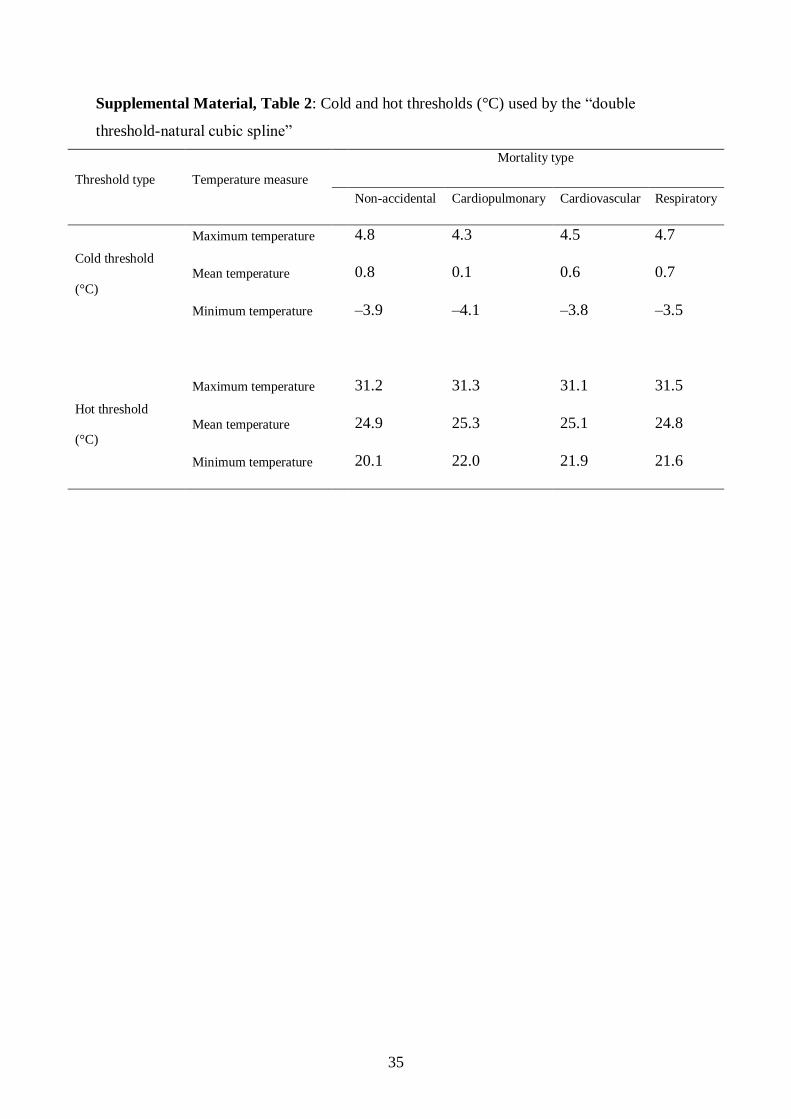
associated with increased mortality by model [1]) were 0.8 °C and 24.9 °C for non-accidental

mortality, 0.1°C and 25.3 °C for cardiopulmonary mortality, 0.6 °C and 25.1 °C for

cardiovascular mortality, 0.7 °C and 24.8 °C for respiratory mortality.

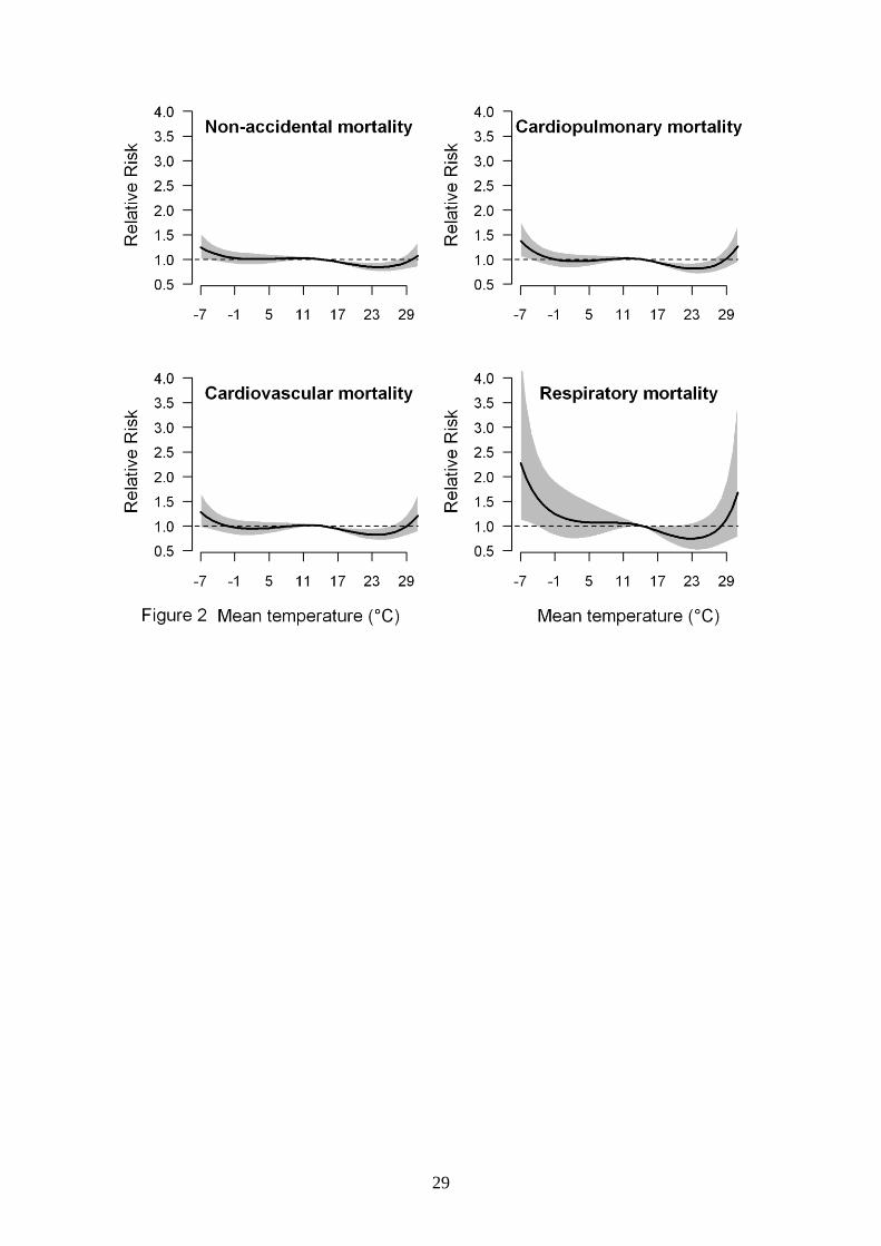
Significant cold effects appeared after after a 3-day lag, while significant hot effects occurred

within 0 to 3 days (Figure 3). Associations between cold and mortality lasted longer than

12

associations with heat. Heat-related excesses of non-accidental, cardiopulmonary, and

cardiovascular mortality were followed by deficits in mortality, consistent with some

mortality displacement caused by hot temperatures.

We calculated the overall effects of mean temperature on non-accidental, cardiopulmonary,

cardiovascular and respiratory mortality along the lags (Table 3). For cold effects over lag 0–

18 days, a 1 °C decrease in mean temperature below the cold thresholds was associated with

a 2.99% (95% confidence interval (CI): 0.85–5.17%) increase in non-accidental deaths,

5.49% (95% CI: 2.29–8.79%) increase in cardiopulmonary deaths, 4.05% (95% CI: 1.14–

7.06%) increase in cardiovascular deaths, and 9.25% (95% CI: 1.70–17.37%) increase in

respiratory deaths. For hot effects over lag 0–2 days, a 1 °C increase in mean temperature

above the hot thresholds was associated with a 2.03% (95% CI: 0.70–3.38%) increase in non-

accidental deaths, 3.04% (95% CI: 1.24–4.87%) increase in cardiopulmonary deaths, 2.80%

(95% CI: 0.95–4.68%) in cardivascular deaths, and 3.36% (95% CI: –0.77 to 7.67%) increase

in respiratory deaths. In general, cold effects of lag 0–27 days were greater than hot effects of

lag 0-27 days except for respiratory mortality.

Sensitivity analysis

We changed the window length of calendar month in the case–crossover to 30, 28, and 21

days, which gave similar results (data not shown). In addition, we changed the maximum lag

to 20 and 30 days, which gave similar results (data not shown). Consequently, we believe that

the models used in this study adequately captured the main effects of temperature on

mortality.

Discussion

13

Temperature-mortality relationship

The temperature-mortality relationship in Tianjin was U-shaped, with a large range of

temperatures that were not associated with excess mortality. Significant associations between

cold temperatures and mortality (cold effects) appeared after 3 days and lasted longer than the

associations between high temperatures and mortality (hot effects), which were acute and of

short duration. There was evidence of some mortality displacement due to effects of high

temperatures on non-accidental, cardiopulmonary, and cardiovascular deaths.

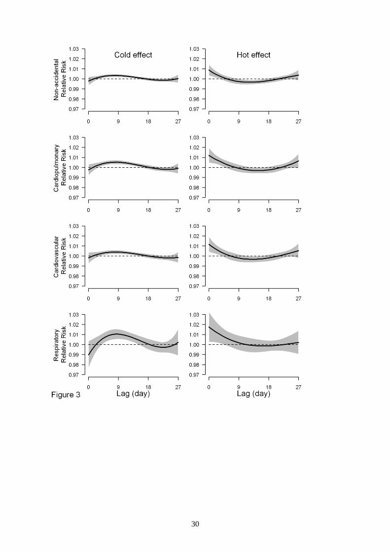
Many studies have examined the temperature-mortality relationship worldwide, but few are

from China (Hajat and Kosatky 2010). We compared our results with studies that examined

both cold and hot effects using mean temperature for non-accidental mortality (Curriero et al.

2002; El-Zein et al. 2004; Revich and Shaposhnikov 2008; Rocklov and Forsberg 2008; Yu

et al. 2011) (Figure 4). Results show that estimated temperature effects varied by region and

population. Compared with populations living at similar latitudes, our results suggest a

stronger cold effect and smaller hot effect. The reason might be that short lags were used in

other studies, while we examined overall cold and hot effects of lag 0–27 days. Studies using

short lags may have underestimated the cold effect, as in our results the estimated cold effect

was delayed by three days and lasted for 10 days. Studies using short lags may overestimate

the hot effect, as in our results there was evidence of some mortality displacement which can

only be captured by using longer lags (Anderson and Bell 2009). Compared with other

median or lower income populations (e.g., Bangkok, Mexico City, São Paulo, Delhi, Santiago,

and Cape Town), Tianjin had lower cold and hot effects. The reason might be that people in

14

Tianjin used protection measures in summer and winter (e.g., air conditioning and heating

system) (McMichael et al. 2008).

We can compare our results with those from similar cities in China. Kan et al. (2003) found a

V-shaped relationship between lag 0–2 days’ temperature and non-accidental mortality in

Shanghai, with an optimum temperature of 26.7 °C. A 1 °C decrease (increase) in

temperature below (above) 26.7 °C increased non-accidental mortality by 1.21% (0.73%).

Liu et al. (2011) found both cold and hot temperatures were associated with increased

cardiopulmonary mortality in Beijing, which has a climate that is similar to Tianjin’s. They

also found an acute and short-term hot effect followed by some mortality displacement for

cardiovascular mortality, consistent with our results.

An interesting finding is that the range of temperatures that are not associated with increased

mortality is quite large in Tianjin, but extreme temperatures still had adverse effects on

mortality. The exchange of heat between the body and surrounding temperature is regulated

constantly by physiological control. Extreme high temperatures may cause a failure of

thermoregulation, which may be impaired by dehydration, salt depletion and increased

surface blood circulation (Bouchama and Knochel 2002). Elevated blood viscosity,

cholesterol levels and sweating thresholds may also be the cause of heat-related mortality

(McGeehin and Mirabelli 2001). Cold temperatures increase the heart rate, peripheral

vasoconstriction, blood pressure, blood cholesterol levels, plasma fibrinogen concentrations,

and platelet viscosity (Ballester et al. 1997; Carder et al. 2005). In Tianjin urban city, eighty-

three percent of houses had central heating in winter (Tianjin Statistic Bureau 2005) and

ninety percent of homes had air conditioners (Tianjin Statistic Bureau 2004). However,

15

although the majority of the urban population were potentially protected from the weather,

there were still some increased risks during extreme cold and hot days.

We investigated lag effects over 28 days on mortality for both hot and cold days. In general,

cold effects lasted about 10 days after the extreme cold days. Previous studies also reported

similarly delayed cold effects on mortality (Anderson and Bell 2009; Goodman et al. 2004).

The findings indicate that using short lags cannot completely capture the cold effect, and so

longer lags are required to examine the cold impact.

The hot effects were more acute and short-term. Studies have shown that hot temperatures

induce an acute event in people with pre-existing diseases (e.g., a previous myocardial

infarction or stroke) and in those who may find it difficult to deal with heat (e.g., the elderly)

(Muggeo and Hajat 2009). In people with congestive heart failure, the extra heat load may

lead to fatal consequences (Näyhä 2005). The hot effect also led mortality displacement for

non-accidental, cardiopulmonary, and cardiovascular deaths, which is in agreement with

studies conducted in Europe (Hajat et al. 2005; Pattenden et al. 2003) and US (Braga et al.

2001). Therefore, using short lags cannot adequately assess the hot effects, as the harvesting

effects were ignored.

Studies of heat-related mortality have examined maximum, mean, or minimum temperatures,

controlling for relative humidity (Anderson and Bell 2009). Other studies have used apparent

temperature, the humidex and temporal synoptic index (Zanobetti and Schwartz 2008). A

large study of mortality in the US found that the different measures of temperature had a

similar ability to predict the impacts of temperature on mortality (Barnett et al. 2010). We

16

found that maximum, mean, and minimum temperatures had similar predictive ability,

probably because of their strong correlation. Overall, mean temperature performed best

according to the AIC.

Case−crossover design and DLNM

Many models have been used to assess the impacts of temperature and air pollution on

mortality and morbidity, such as descriptive (Reid et al. 2009), case-only (Schwartz 2005),

case–crossover (Stafoggia et al. 2006), time-series (Hajat et al. 2002) and spatial analysis

(Vaneckova et al. 2010). Generally, time-series and case–crossover designs are the most

commonly used in a single or in multiple locations over a time period. The main aim of both

analyses is to examine associations between health and temperature, after controlling for

potential confounding factors such as secular trends and seasonal cycles (Basu et al. 2005).

Using the case–crossover design each subject is their own control, and so any confounding by

fixed characteristics is removed. Another advantage of the case-crossover is that it controls

for long-term and seasonal trends by design through short-interval strata (e.g. calendar

month).

We compared the case–crossover design and a time series design using a natural cubic spline

with 7 degrees of freedom for time per year. The case–crossover design performed better than

time series analysis for this particular data based on AIC and residuals. However, we cannot

conclude the case–crossover is better than time series for other data. We suggest checking the

model fit and residuals when using case–crossover or time series designs. In this study, we

illustrated how to combine the DLNM with a case−crossover design. This allows

17

sophisticated non-linear and delayed temperatures to be fitted using the case−crossover

design.

One of the main advantages of DLNM is that it allows the model to contain detailed lag

effects of exposure on response, and provides the estimate of the overall effect that is

adjusted for harvesting (Gasparrini et al. 2010). The DLNM can flexibly show different

temperature-mortality relationships for lags using different smoothing functions. The DLNM

can adequately model the main effects of temperature (Armstrong 2006).

There are also some issues in the selection of the DLNM, such as cross-basis type, maximum

lag day, and degrees of freedom (knots and placement) for exposure and lag (Armstrong 2006;

Gasparrini et al. 2010). Because the DLNM is combined with a regression model (e.g.,

Poisson regression), the residual deviance and autocorrelation plot, maximum likelihood,

Akaike’s information criteria or Bayesian information criteria can be used to check the model.

The options for the DLNM can be chosen according to the best model fit. Previous studies

recommend choosing a DLNM that is easy to interpret from an epidemiological perspective

(Armstrong 2006; Gasparrini et al. 2010). However, it is necessary to conduct sensitivity

analyses to assess the key conclusions on model choice. In this study, we used AIC to select

the degrees of freedom, and used residual deviance to choose both cold and hot thresholds,

but used a priori arguments to choose cross-basis type and maximum lag day.

Strengths and limitations

18

This is the first study to give details on how to apply a DLNM in the case−crossover design,

and the first to assess the temperature-mortality relationship in Tianjin, China. We examined

both cold and hot lag effects on four types of mortality, and explored which temperature

measure was the best predictor of mortality. Our findings can be used to promote capacity

building for local response for extreme temperatures.

A limitation is that the data are only from one city, so it is difficult to generalise our results to

other cities or to rural areas. We used the data on temperature and air pollution from fixed

sites rather than individual exposure, so there may be some inevitable measurement error.

The influence of ozone was not controlled for, because data on ozone were unavailable. In

previous research, hot effects were slightly reduced when ozone was controlled for, but cold

effects were not changed (Anderson and Bell 2009). Some studies found a potential

interaction between temperature and ozone (Ren et al. 2008). Further study needs to be

conducted for this issue.

Conclusions

DLNM can be applied in a case−crossover design, so that the case−crossover can be used to

examine sophisticated non-linear and delayed effects of exposure (e.g., temperature or air

pollution). Even though there was a relatively large temperature range that was not associated

with excess mortality, extreme cold and hot temperatures were associated with an increased

risk of mortality in Tianjin, China. Cold temperatures had longer lasting effects on mortality,

while hot temperatures had acute and short-term effects.

19

References

Analitis A, Katsouyanni K, Biggeri A, Baccini M, Forsberg B, Bisanti L, et al. 2008. Effects

of cold weather on mortality: results from 15 European cities within the PHEWE

project. Am J Epidemiol 168(12):1397-1408.

Anderson BG, Bell ML. 2009. Weather-related mortality: how heat, cold, and heat waves

affect mortality in the United States. Epidemiology 20(2):205-213.

Armstrong B. 2006. Models for the relationship between ambient temperature and daily

mortality. Epidemiology 17(6):624-631.

Baccini M, Biggeri A, Accetta G, Kosatsky T, Katsouyanni K, Analitis A, et al. 2008. Heat

effects on mortality in 15 European cities. Epidemiology 19(5):711-719.

Ballester F, Corella D, Perez-Hoyos S, Saez M, Hervas A. 1997. Mortality as a function of

temperature, a study in Valencia, Spain, 1991-1993. International Journal of

Epidemiology 26(3):551-561.

Barnett AG, Dobson AJ. 2010. Analysing Seasonal Health Data. Berlin, Heidelberg: Springer.

Barnett AG, Tong S, Clements ACA. 2010. What measure of temperature is the best

predictor of mortality? Environmental Research 110(6):604-611.

Basu R, Dominici F, Samet JM. 2005. Temperature and mortality among the elderly in the

United States: a comparison of epidemiologic methods. Epidemiology 16(1):58-66.

Basu R, Feng WY, Ostro BD. 2008. Characterizing temperature and mortality in nine

California counties. Epidemiology 19(1):138-145.

Bouchama A, Knochel JP. 2002. Heat stroke. N Engl J Med 346(25):1978-1988.

Braga AL, Zanobetti A, Schwartz J. 2001. The time course of weather-related deaths.

Epidemiology 12(6):662-667.

20

Carder M, McNamee R, Beverland I, Elton R, Cohen GR, Boyd J, et al. 2005. The lagged

effect of cold temperature and wind chill on cardiorespiratory mortality in Scotland.

Occup Environ Med 62(10):702-710.

Chan EY, Goggins WB, Kim JJ, Griffiths SM. 2010. A study of intracity variation of

temperature-related mortality and socioeconomic status among the Chinese population

in Hong Kong. J Epidemiol Community Health.

Curriero FC, Heiner KS, Samet JM, Zeger SL, Strug L, Patz JA. 2002. Temperature and

mortality in 11 cities of the eastern United States. Am J Epidemiol 155(1):80-87.

Ebi KL, Kovats RS, Menne B. 2006. An approach for assessing human health vulnerability

and public health interventions to adapt to climate change. Environ Health Perspect

114(12):1930-1934.

El-Zein A, Tewtel-Salem M, Nehme G. 2004. A time-series analysis of mortality and air

temperature in Greater Beirut. Sci Total Environ 330(1-3):71-80.

Gasparrini A, Armstrong B. 2011. Distributed lag non-linear models in R: the package dlnm.

Gasparrini A, Armstrong B, Kenward MG. 2010. Distributed lag non-linear models. Stat Med

29(21):2224-2234.

Goodman PG, Dockery DW, Clancy L. 2004. Cause-Specific Mortality and the Extended

Effects of Particulate Pollution and Temperature Exposure. Environmental Health

Perspectives 112(2):179-185.

Green RS, Basu R, Malig B, Broadwin R, Kim JJ, Ostro B. 2010. The effect of temperature

on hospital admissions in nine California counties. Int J Public Health 55(2):113-121.

Group E. 1997. Cold exposure and winter mortality from ischaemic heart disease,

cerebrovascular disease, respiratory disease, and all causes in warm and cold regions of

Europe. The Eurowinter Group. Lancet 349(9062):1341-1346.

21

Hajat S, Kosatky T. 2010. Heat-related mortality: a review and exploration of heterogeneity.

J Epidemiol Community Health 64(9):753-760.

Hajat S, Kovats RS, Atkinson RW, Haines A. 2002. Impact of hot temperatures on death in

London: a time series approach. Journal of Epidemiology and Community Health,367-

372.

Hajat S, Armstrong BG, Gouveia N, Wilkinson P. 2005. Mortality displacement of heat-

related deaths: a comparison of Delhi, Sao Paulo, and London. Epidemiology

16(5):613-620.

Janes H, Sheppard L, Lumley T. 2005. Overlap bias in the case-crossover design, with

application to air pollution exposures. Stat Med 24(2):285-300.

Kan HD, Jia J, Chen BH. 2003. Temperature and daily mortality in Shanghai: a time-series

study. Biomed Environ Sci 16(2):133-139.

Liu L, Breitner S, Pan X, Franck U, Leitte A, Wiedensohler A, et al. 2011. Associations

between Air Temperature and Cardio-Respiratory Mortality in the Urban Area of

Beijing, China: A Time-Series Analysis. Environmental Health 10(1):51.

Lu Y, Zeger SL. 2007. On the equivalence of case-crossover and time series methods in

environmental epidemiology. Biostatistics 8(2):337-344.

Lu Y, Symons JM, Geyh AS, Zeger SL. 2008. An approach to checking case-crossover

analyses based on equivalence with time-series methods. Epidemiology 19(2):169-175.

McGeehin M, Mirabelli M. 2001. The potential impacts of climate variability and change on

temperature-related morbidity and mortality in the United States. Environmental Health

Perspectives 109(Suppl 2):185-189.

McMichael AJ, Wilkinson P, Kovats RS, Pattenden S, Hajat S, Armstrong B, et al. 2008.

International study of temperature, heat and urban mortality: the 'ISOTHURM' project.

Int J Epidemiol 37(5):1121-1131.

22

Muggeo VM, Hajat S. 2009. Modelling the non-linear multiple-lag effects of ambient

temperature on mortality in Santiago and Palermo: a constrained segmented distributed

lag approach. Br Med J 66(9):584-591.

Näyhä S. 2005. Environmental temperature and mortality. Int J Circumpolar Health

64(5):451-458.

Pattenden S, Nikiforov B, Armstrong BG. 2003. Mortality and temperature in Sofia and

London. J Epidemiol Community Health 57(8):628-633.

Peng RD, Dominici F, Louis TA. 2006. Model choice in time series studies of air pollution

and mortality. Journal of the Royal Statistical Society: Series A (Statistics in Society)

169(2):179-203.

Reid C, O’Neill M, Gronlund C, Brines S, Brown D, Diez-Roux A, et al. 2009. Mapping

community determinants of heat vulnerability. Environ Health Perspect 117(11):1730-

1736.

Ren C, Williams GM, Morawska L, Mengersen K, Tong S. 2008. Ozone modifies

associations between temperature and cardiovascular mortality: analysis of the

NMMAPS data. Occup Environ Med 65(4):255-260.

Revich B, Shaposhnikov D. 2008. Temperature-induced excess mortality in Moscow, Russia.

Int J Biometeorol 52(5):367-374.

Rocklov J, Forsberg B. 2008. The effect of temperature on mortality in Stockholm 1998--

2003: a study of lag structures and heatwave effects. Scand J Public Health 36(5):516-

523.

Schwartz J. 2005. Who is sensitive to extremes of temperature?: A case-only analysis.

Epidemiology 16(1):67.

23

Stafoggia M, Schwartz J, Forastiere F, Perucci CA. 2008. Does temperature modify the

association between air pollution and mortality? A multicity case-crossover analysis in

Italy. Am J Epidemiol 167(12):1476-1485.

Stafoggia M, Forastiere F, Agostini D, Biggeri A, Bisanti L, Cadum E, et al. 2006.

Vulnerability to heat-related mortality: a multicity, population-based, case-crossover

analysis. Epidemiology 17(3):315-323.

Tianjin Statistic Bureau. 2004. Tianjin Statistical Bulletin. http://www.stats-

tj.gov.cn/Article/tjgb/stjgb/200612/5371.html.

Tianjin Statistic Bureau. 2005. Tianjin Statistical Bulletin. http://www.stats-

tj.gov.cn/Article/tjgb/stjgb/200612/5375.html.

Vaneckova P, Beggs PJ, Jacobson CR. 2010. Spatial analysis of heat-related mortality among

the elderly between 1993 and 2004 in Sydney, Australia. Soc Sci Med 70(2):293-304.

World Health Organization. 2007. International Statistical Classification of Diseases and

Related Health Problems, 10th Revision, Version for 2007.

Yu W, Mengersen K, Hu W, Guo Y, Pan X, Tong S. 2011. Assessing the relationship

between global warming and mortality: Lag effects of temperature fluctuations by age

and mortality categories. Environ Pollut 159(7):1789-1793.

Zanobetti A, Schwartz J. 2008. Temperature and mortality in nine US cities. Epidemiology

19(4):563-570.

24

Table 1: Summary statistics of daily weather conditions and mortality in Tianjin, China,

2005–2007

Variables Minimum 25% Median 75% Maximum Mean SD

Maximum temperature (°C) –6 8 21 30 40 19 12

Mean temperature (°C) –11 3 14 24 31 13 11

Minimum temperature (°C) –14 –2 10 19 29 8 11

Humidity (%) 13 46 61 74 97 60 19

Non-accidental death 26 46 55 66 106 56 14

Cardiopulmonary death 13 27 33 40 77 34 9

Cardiovascular death 9 24 29 35 67 30 8

Respiratory death 0 3 4 6 15 4 2

Influenza death 0 0 0 0 2 0 0.1

SD = standard deviation

25

Table 2: Spearman’s correlation coefficients between weather conditions in Tianjin, China,

2005–2007

Temperature measures Mean

temperature

Minimum

temperature

Humidity

Maximum temperature 0.98** 0.94** 0.16*

Mean temperature 0.98** 0.24*

Minimum temperature 0.32*

*P<0.05

**P<0.01

26

Table 3: The cumulative cold and hot effects of mean temperature on mortality categories

along the lag days, using a “double threshold-natural cubic spline” DLNM with 4 degrees of

freedom natural cubic spline for lag.

Effects

Lag

(days)

% increase in mortality (95% CI)

Non-accidental Cardiopulmonary Cardiovascular Respiratory

Cold effect a 0–2 –0.27 (–1.25, 0.72) –0.19 (–1.49, 1.12) –0.14 (–1.43, 1.17) –1.65 (–4.75, 1.55)

0–18 2.99 (0.85, 5.17)* 5.49 (2.29, 8.79)* 4.05 (1.14, 7.06)* 9.25 (1.70, 17.37)*

0–27 2.13 (–0.44, 4.78) 4.16 (0.27, 8.21)* 2.66 (–0.86, 6.30) 7.99 (–1.08, 17.9)

Hot effect b 0–2 2.03 (0.70, 3.38)* 3.04 (1.24, 4.87)* 2.80 (0.95, 4.68)* 3.36 (–0.77, 7.67)

0–18 –0.78 (–4.20, 2.77) 2.32 (–2.59, 7.49) 0.86 (–4.02, 5.98) 8.60 (–2.78, 21.31)

0–27 0.31 (–3.48, 4.24) 3.83 (–1.75, 9.72) 2.47 (–2.99, 8.24) 8.79 (–3.62, 22.80)

*P<0.05

a The percent increase in mortality for a 1 °C of temperature decrease below the cold

thresholds (0.8 °C for non-accidental, 0.1 °C for cardiopulmonary 0.6 °C for cardiovascular,

and 0.7 °C respiratory mortality).

b The percent increase in mortality for a 1 °C of temperature increase above the hot thresholds

(24.9 °C for non-accidental, 25.3 °C for cardiopulmonary 25.1 °C for cardiovascular, and

24.8 °C for respiratory mortality).

27

Figure legend:

Figure 1: Relative risks of mortality types by mean temperature (°C), using a “natural cubic

spline-natural cubic spline” DLNM with 5 degrees of freedom natural cubic spline for

temperature and 4 degrees of freedom for lag.

Figure 2: The estimated overall effects of mean temperature (°C) over 28 days on mortality

types, using a “natural cubic spline-natural cubic spline” DLNM with 5 degrees of freedom

natural cubic spline for temperature and 4 degrees of freedom for lag. The black lines are the

mean relative risks, and the grey regions are 95% confidence intervals.

Figure 3: The estimated effects of a 1 °C decrease in mean temperature below the cold

threshold (left) and of a 1 °C increase in mean temperature above the hot threshold (right) on

mortality types over 27 days of lag, using a “double threshold-natural cubic spline” DLNM

with 4 degrees of freedom natural cubic spline for lag. The black lines are mean relative risks,

and grey regions are 95% confidence intervals. The cold and hot thresholds were 0.8 °C and

24.9 °C for non-accidental mortality, 0.1°C and 25.3 °C for Cardiopulmonary mortality,

0.6 °C and 25.1 °C for cardiovascular mortality, 0.7 °C and 24.8 °C for respiratory mortality.

Figure 4: Comparison of the impacts of temperature on non-accidental mortality in different

populations ordered by latitude.

28

29

30

31

32

Supplemental Material

The Impact of Temperature on Mortality in Tianjin, China: A Case–

crossover Design with A Distributed Lag Non-linear Model

Yuming Guo1, Adrian G Barnett

1, Xiaochuan Pan

2, Weiwei Yu

1, Shilu Tong

1

1 School of Public Health and Institute of Health and Biomedical Innovation, Queensland

University of Technology, Brisbane, Australia.

2 School of Public Health, Peking University, Beijing, China.

33

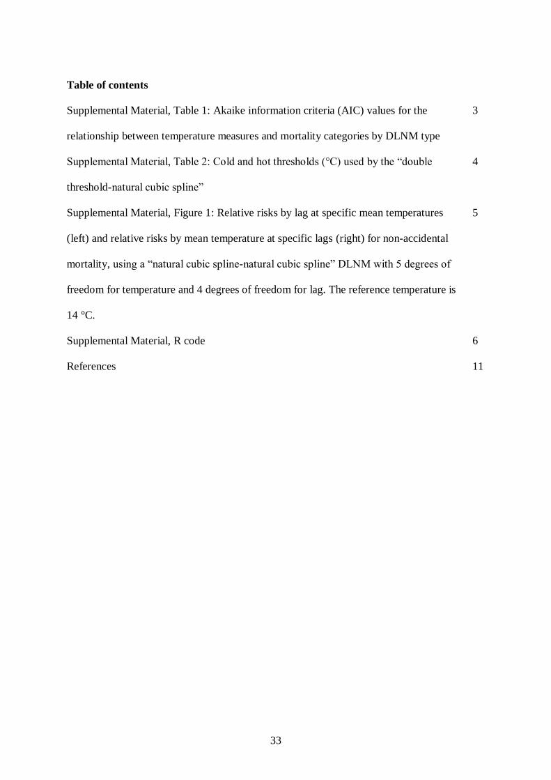
Table of contents

Supplemental Material, Table 1: Akaike information criteria (AIC) values for the

relationship between temperature measures and mortality categories by DLNM type

3

Supplemental Material, Table 2: Cold and hot thresholds (°C) used by the “double

threshold-natural cubic spline”

4

Supplemental Material, Figure 1: Relative risks by lag at specific mean temperatures

(left) and relative risks by mean temperature at specific lags (right) for non-accidental

mortality, using a “natural cubic spline-natural cubic spline” DLNM with 5 degrees of

freedom for temperature and 4 degrees of freedom for lag. The reference temperature is

14 °C.

5

Supplemental Material, R code 6

References 11

34

Supplemental Material, Table 1: Akaike information criteria (AIC) values for the

relationship between temperature measures and mortality categories by DLNM type

DLNM type Temperature measure

AIC

Non-accidental Cardiopulmonary Cardiovascular Respiratory

Natural cubic

spline-natural

cubic spline a

Maximum temperature 7494 6860 6679 4562

Mean temperature 7472 6841 6658 4570

Minimum temperature 7472 6840 6660 4580

Double threshold-

natural cubic

spline b

Maximum temperature 7488 6849 6662 4568

Mean temperature 7473 6833 6653 4558

Minimum temperature 7481 6845 6666 4556

a Using “natural cubic spline-natural cubic spline” DLNM with smoothing of 5 degrees of

freedom for temperature and 4 degrees of freedom for lag;

b Using “double threshold-natural cubic spline” DLNM with smoothing of 4 degrees of

freedom for lag; the cold and hot thresholds are shown in Supplemental Material, Table 2.

35

Supplemental Material, Table 2: Cold and hot thresholds (°C) used by the “double

threshold-natural cubic spline”

Threshold type Temperature measure

Mortality type

Non-accidental Cardiopulmonary Cardiovascular Respiratory

Cold threshold

(°C)

Maximum temperature 4.8 4.3 4.5 4.7

Mean temperature 0.8 0.1 0.6 0.7

Minimum temperature –3.9 –4.1 –3.8 –3.5

Hot threshold

(°C)

Maximum temperature 31.2 31.3 31.1 31.5

Mean temperature 24.9 25.3 25.1 24.8

Minimum temperature 20.1 22.0 21.9 21.6

36

1

Supplemental Material, Figure 1: Relative risks by lag at specific mean temperatures (left) 2

and relative risks by mean temperature at specific lags (right) for non-accidental mortality, 3

using a “natural cubic spline-natural cubic spline” DLNM with 5 degrees of freedom for 4

temperature and 4 degrees of freedom for lag. The reference temperature is 14 °C. 5

6

37

7

Supplemental Material, R code 8

9

As our data from Tianjin is not publicly available, we used data from Jersey city as an 10

example. The data were from the National Morbidity, Mortality, and Air Pollution Study 11

(NMMAPS) (Samet et al. 2000a; Samet et al. 2000b). 12

13

1. Load packages and prepare dataset: 14

>library(dlnm); library (NMMAPSlite) 15

>initDB() 16

>cities <- listCities() 17

# Jersey City: jers (city number 43) 18

>data <- readCity(cities[43], collapseAge = TRUE) 19

>data <- data[,c("city","date","death","inf","tmpd","rhum","so2mean","pm10trend")] 20

>data$temp <- (data$tmpd-32)*5/9 # Transfer temperature to Celsius 21

>data$time<-1:length(data[,1]) # Create time 22

>data$dow<-as.numeric(format(data$date,"%w")) # Create day of the week 23

>data$year<-as.numeric(format(data$date,"%Y")) # Create year 24

>data$month<-as.numeric(format(data$date,"%m")) # Create month 25

>data$strata<-data$year*100+data$month # Case-Control strata 26

27

2. Create Cross-basis matrix using “natural cubic spline-natural cubic spline” DLNM 28

with 5 df for temperature and 4 df for lag 29

>range <- range(data$temp,na.rm=T) 30

>nknots<-4 # Number of knots for temperature 31

>nlagknots<-2 # Number of knots for lag 32

>ktemp <- range[1] + (range[2]-range[1])/(nknots+1)*1:nknots # Knots for temperature 33

>klag<-exp((log(27))/(nlagknots+2)*1:nlagknots) # Knots for lag 34

>basis.temp <- crossbasis(data$temp, vartype="ns", varknots=ktemp, 35

cenvalue=median(data$temp,na.rm=T), lagtype="ns", lagknots=klag,maxlag=27) 36

37

3. Combine the case-crossover design with DLNM 38

>model.month <- glm(death ~ basis.temp + ns(rhum,df=3) + ns(pm10trend,df=3) + 39

38

ns(so2mean,df=3) + as.factor(I(inf>0)) + as.factor(strata)+as.factor(dow), 40

family=quasipoisson(), data) 41

42

4. Derive the predicted effects and standard errors for temperature and lags using 43

DLNM 44

>pred.month <- crosspred(basis.temp, model.month, at=-16:32) 45

46

5. Plot 3D and overall effect graphics 47

> plot (pred.month,"3d",zlab="Relative Risk", r=90, d=0.3, col="red", xlab="Temperature", 48

main="3D graphic for Jersey City", expand=0.6,lwd=0.5) 49

>plot(pred.month,"overall", xlab="Temperature (°C)", ylab=" Relative Risk ", 50

main="Overall effect of temperature on mortality\n between 1987-2000 for Jersey City") 51

52

6. Determine the cold and hot thresholds (in °C) using “double threshold-natural cubic 53

spline” DLNM 54

Based on the above 3D plot and overall effect plot, there are two potential thresholds for 55

temperature. The cold threshold is somewhere between 0 to 8 °C, and hot threshold is 56

somewhere between 19 to 26 °C. We used the following models to determine which 57

combination of cold and hot thresholds gave the lowest residual deviance. 58

59

>cold.thr<-0:8 # In 1°C increments (In our study, we used 0.1°C increments) 60

>hot.thr<-19:26 # In 1°C increments (In our study, we used 0.1°C increments) 61

>deviance.matrix<-matrix(data = NA, nrow = length(cold.thr), ncol = length(hot.thr), byrow 62

= FALSE, dimnames = list(paste("cold.thr", cold.thr,sep="."), 63

paste("hot.thr", hot.thr,sep="."))) 64

>for (i in 1:length(cold.thr)){ 65

for (j in 1:length(hot.thr)){ 66

basis.try <- crossbasis(data$temp, vartype="dthr",varknots=c(cold.thr[i],hot.thr[j]), 67

lagtype="ns", lagknots=klag, maxlag=27) 68

model <- glm(death ~ basis.try + ns(rhum,df=3) + ns(pm10trend,df=3) + ns(so2mean,df=3) 69

+ as.factor(I(inf>0)) + as.factor(strata)+as.factor(dow), family=quasipoisson(), data) 70

deviance.matrix[i,j]<-model$deviance 71

} 72

39

} 73

>row.col <- arrayInd(which.min(deviance.matrix), dim(deviance.matrix)) 74

>rowname<-rownames(deviance.matrix)[row.col[,1]] 75

>colname<-colnames(deviance.matrix)[row.col[,2]] 76

>rowname;colname # Get the cold and hot thresholds 77

[1] "cold.thr.4" # The best cold threshold is 4°C 78

[1] "hot.thr.22" # The best hot threshold is 22 °C 79

80

7. Examine the cold (hot) effects below (above) the cold (hot)threshold using “Double 81

threshold-natural cubic spline” DLNM 82

The cold threshold 4 °C and hot threshold 22 °C are used for a “Double threshold-natural 83

cubic spline” DLNM. 84

>basis.cold.hot<- crossbasis(data$temp, vartype="dthr",varknots=c(4,22), 85

lagtype="ns", lagknots=klag, maxlag=27) 86

>model.cold.hot <- glm(death ~ basis.cold.hot + ns(rhum,df=3) + ns(pm10trend,df=3) + 87

ns(so2mean,df=3) + as.factor(I(inf>0)) + as.factor(strata)+as.factor(dow), 88

family=quasipoisson(), data) 89

>cold.hot.pred <- crosspred(basis.cold.hot,model.cold.hot,at=-16:32) 90

> plot(cold.hot.pred,"3d",zlab="Relative Risk", r=90,d=0.3,col="red",xlab="Temperature", 91

main="\n3D graphic for Jersey City\nfor double threshold",expand=0.6,lwd=0.5) # 3D plot 92

93

>par(mfrow=c(2,1)) 94

>plot(cold.hot.pred,"slices",var=c(3),main="Cold effect", xlab="", ylab=" Relative Risk ", 95

ylim=range(0.99,1.01)) 96

>plot(cold.hot.pred,"slices",var=c(23),main="Hot effect",xlab="Lag (day)", 97

ylab=" Relative Risk", ylim=range(0.99,1.01)) 98

99

8. Sensitivity analysis using 20 days as the maximum lag 100

> nlagknots<-2 # Number of knots for lag 101

> klag.20<-exp(log(20)/(nlagknots+2)*1:nlagknots) # Knots for lag 102

> basis.temp.20 <- crossbasis(data$temp, vartype="ns", varknots=ktemp, 103

cenvalue=median(data$temp,na.rm=T), lagtype="ns",lagknots=klag.20,maxlag=20) 104

> model.month.20 <- glm(death ~ basis.temp.20 + ns(rhum,df=3) + ns(pm10trend,df=3) + 105

40

ns(so2mean,df=3) + as.factor(I(inf>0)) +as.factor(strata)+as.factor(dow), 106

family=quasipoisson(), data) 107

> pred.month.20 <- crosspred(basis.temp.20, model.month.20, at=-16:32) 108

> plot(pred.month.20,"overall", xlab="Temperature (°C)", ylab="Relative risk", 109

main="Overall effect of temperature on mortality\n between 1987-2000 for Jersey 110

City using maximum lag of 20 days") 111

112

9. Sensitivity analysis using 30 days as strata 113

>strata30<-floor((data$time-min(data$time))/30) # Create strata as 30 days 114

>model.strata30<- glm(death ~ basis.temp + ns(rhum,df=3) + ns(pm10trend,df=3) + 115

ns(so2mean,df=3) + as.factor(I(inf>0)) +as.factor(strata30)+as.factor(dow), 116

family=quasipoisson(), data) 117

>pred.strata30<- crosspred(basis.temp, model.strata30, at=-16:32, cumul=T) 118

>plot(pred.strata30,"overall", xlab="Temperature (°C)", ylab=" Relative risk ", 119

main="Overall effect of temperature on mortality\n between 1987-2000 for Jersey 120

City using 30 days as strata") 121

122

10. Comparison of time series and case–crossover design 123

# ignore humidity & pollution to remove influence of missing values 124

# case-crossover using calendar month as strata 125

>model.month <- glm(death ~ basis.temp + as.factor(I(inf>0)) 126

+as.factor(strata)+as.factor(dow), family=quasipoisson(), data) 127

128

# time series with 7 degrees of freedom for time per year 129

>model.ts <- glm(death ~ basis.temp + as.factor(I(inf>0)) +ns(time,98)+as.factor(dow), 130

family=quasipoisson(), data) 131

132

# Plot the residual distribution 133

>par(mfrow=c(2,1)) 134

> hist(resid(model.month),main="Residual distribution for case-crossover design\nusing 135

calendar month as strata", xlim=range(-4,5),ylim=range(0,1100),xlab="Residuals",col="red", 136

font.lab=2,las=1) 137

41

>hist(resid(model.ts),main="Residual distribution for time series design\nusing 7 df for time 138

per year", xlim=range(-4,5),ylim=range(0,195),xlab="Residuals",col="red",font.lab=2,las=1) 139

>par(mfrow=c(1,1)) 140

141

# Calculate AIC value for case-crossover 142

>AIC.cc<- -2*sum( dpois( model.month$y, model.month$fitted.values, log=TRUE))+ 143

2*summary(model.month)$df[3]*summary(model.month)$dispersion 144

AIC.cc="26364.29" 145

146

# Calculate AIC value for time series 147

>AIC.ts <- -2*sum( dpois( model.ts $y, model.ts $fitted.values, log=TRUE))+ 148

2*summary(model.ts )$df[3]*summary(model.ts )$dispersion 149

AIC.ts =" 26297.70" 150

151

For Jersey City, a time series design performs better than case-crossover as judged by the 152

AIC. However, both designs give similar residuals. (For Tianjin, a case–crossover performed 153

better than a time series according to both the AIC and residuals) 154

155

156

42

References 157

Samet JM, Dominici F, Zeger SL, Schwartz J, Dockery DW. 2000a. The National Morbidity, 158

Mortality, and Air Pollution Study. Part I: Methods and methodologic issues. Res Rep 159

Health Eff Inst(94 Pt 1): 5-14; discussion 75-84. 160

Samet JM, Zeger SL, Dominici F, Curriero F, Coursac I, Dockery DW, et al. 2000b. The 161

National Morbidity, Mortality, and Air Pollution Study. Part II: Morbidity and 162

mortality from air pollution in the United States. Res Rep Health Eff Inst 94(Pt 2): 5-70; 163

discussion 71-79. 164

165

166

167